Discrimination in the Labor Market: The Curse of ...Discrimination in the Labor Market: The Curse of...

Discrimination in the Labor Market: The Curse of

Competition between Workers

Thomas de Haan, Theo Offerman and Randolph Sloof∗

University of Amsterdam and Friedrich Schiller University Jena

November 20, 2013

Abstract

In an experiment we identify a crucial factor that determines whether employ-

ers engage in statistical discrimination of ex-ante equal groups. In the stan-

dard no-competition setup of Coate and Loury (1993), we do not find system-

atic evidence for statistical discrimination. When we introduce competition

between workers of different groups for the same job, the non-discrimination

equilibrium ceases to be stable. In line with this theoretical observation, we

find systematic discrimination in the experimental treatment with competi-

tion. Nevertheless, a substantial minority of the employers refuses to discrim-

inate even when it is in their best interest to do so.

Keywords: Statistical discrimination, labor market, competition, experi-

ment

JEL codes: J71, D82, C91

∗De Haan: Friedrich Schiller University Jena and the Max Planck Institute of Economics.Offerman and Sloof: Amsterdam School of Economics, University of Amsterdam, Roetersstraat 11,1018 WB Amsterdam, the Netherlands. This research was sponsored by the Research Priority AreaBehavioral Economics. We are very grateful to CREED programmer Jos Theelen for programmingthe experiment. We would like to thank seminar audiences at New York University, TilburgUniversity, University of California at Santa Barbara and University of California at San Diego forhelpful comments.

1 Introduction

World-wide, gender and race are ongoing factors determining whether a person

gets a job or not, and whether a person receives a fair wage or not. Even though

gender differences declined in the 1980s and 1990s, sizable differences remain between

male and female wages and in the relative presence of women in the highest paid

jobs. Racial inequality is a persistent phenomenon in many countries as well. For

instance, Dutch workers from Moroccan descent are almost three times as likely to

be unemployed compared to autochthonous Dutch (CBS, 2010).1

In this paper, we contribute to the understanding of how labor market discrim-

ination may arise even when groups are originally equally skilled. Such knowledge

is essential to successfully fight discrimination, because different forms of discrimi-

nation may require different treatments. Broadly speaking, economists have offered

two lines of explanation for discrimination in the labor market. One possibility

is that the origin of discrimination is taste-based (Becker, 1971). According to the

standard interpretation, employers sacrifice profit by treating some group of workers

worse, simply because they dislike them. The other possibility is that the differen-

tial treatment of groups is rooted in statistical discrimination (Phelps, 1972; Arrow,

1973; Coate and Loury, 1993; Fryer and Loury, 2005). Statistical discrimination

occurs when employers’ beliefs that the productivity of demographic groups dif-

fers induce these groups to behave differently, such that the employers’ beliefs are

supported by the data.

Statistical discrimination is a potentially more persistent problem than taste-

based discrimination, because the former can persist in equilibrium while the latter

may be eroded by competitive market forces.2 Even though plausible stories of

statistical discrimination have been proposed, it has not yet been possible to en-

dogenously create statistical discrimination among equally skilled groups in the lab-

oratory.3 In an experiment that straightforwardly implements the model of Coate

1Examples of empirical studies investigating unequal treatment in the labor marker includeBlau and Kahn (1992, 2003), Goldin and Rouse (2000), Azmat, Guell and Manning (2006) andArulampalam, Booth and Bryan (2007). For overviews, see Darity and Mason (1998) and Altonjiand Blank (1999).

2Taste-based discrimination may survive in some niches of the labor market though. For in-stance, if customers have a taste for discrimination and are willing to pay to be served by workersfrom a certain group, employers may hire employees in accordance with the customers’ tastes; seeAkerlof and Kranton (2010) for a discussion of such examples.

3As we will explain in detail below, we add competition between workers to the setup of Coateand Loury (1993). In contrast, Phelps (1972) proposes a model where available productivity mea-sures are noisier for minority workers. So ex-ante the groups are not equal. Arrow (1973) describesa model of statistical discrimination where employers offer lower wages to minorities. In contrastto Arrow, we focus on discrimination in job assignment, arguably the form of discrimination thatis harder to detect and fight. Fryer and Loury (2005) study discrimination in a model where

1

and Loury (1993), Fryer, Goeree and Holt (2005) do not find evidence of systematic

statistical discrimination.

In the world of Coate and Loury, on a certain market day an employer receives

a single application from a worker of either of two groups. The employer hires the

worker if he is sufficiently sure that the worker has invested in her own quality.4

The insight of Coate and Loury is that the game has multiple equilibria, so it may

happen that the employer plays according to one equilibrium with one group and

according to another equilibrium with the other group. In this case discrimination

occurs. Yet it is also possible that the employer uses the same standard to judge

workers from the two groups, preventing the occurrence of discrimination.

In the original model of Coate and Loury, potential discrimination is explained

as the result of two groups reaching a different outcome of a coordination game.

Essentially, the two groups of workers are treated independently by the employers,

as if they live on separate “islands” (Moro and Norman, 2004). A restrictive feature

of the model is that there is no interaction between the two groups of workers. In

particular, higher investments in quality by one group do not put the other group

at a disadvantage. This element is present in recent theoretical models by Mailath,

Samuelson and Shaked (2000), Moro and Norman (2004) and Yoo (2010). In their

models, workers from different groups engage in direct competition and thus may

suffer or benefit from each others’ behavior.5

More realistic as they are, the existing models with competition shed little light

on the question which equilibrium will ultimately materialize under what circum-

stances. The novel insight of our paper is that the equilibrium where workers are

not discriminated may become unstable if workers of different groups compete for

the same job, as typically happens when an employer advertises one vacancy and

receives multiple applications. In contrast, without competition between workers,

there is no destabilizing force if employers refrain from discriminating.

Notice what happens if there are arbitrarily small differences in the historical

rates according to which the two groups invest in their own quality. If there is no

competition between workers, as in the original Coate-Loury model, the employer

may hire the worker of either group because each group’s investment rate is above

the critical threshold. Or vice versa, he may not hire any worker because both in-

vestment levels are below the threshold. If there is competition for the same job and

two groups compete in a tournament-like structure. Their approach differs for instance in theirassumption about ex-ante differences between the groups.

4We will use the arbitrary convention that the employer is male and the worker is female.5Chaudhuri and Sethi (2008) study peer group effects in the (in their model endogenous) costs

of acquiring human capital as another driver of spillovers between groups.

2

at most one of the applicants will be offered the job in question, the situation differs

dramatically. Now a small difference in the historical investment rates of the two

groups will have a profound effect, because all other things equal the employer will

hire a worker from the group with the slightly higher investment rate. With compe-

tition, small differences in historical investment rates thus have a strong impact on

the employer’s behavior, which discourages further investments of the disadvantaged

group.

In a laboratory experiment, we investigate the validity of our theoretical ar-

gument that competition between workers drives statistical discrimination.6 We

illustrate the argument in a simple model. In an experiment, we find clear support

for our intuition. That is, we find substantial discrimination when workers of dif-

ferent groups apply for the same job but hardly any discrimination without such

competition.

There is one striking difference between our experimental data and the pre-

dictions from the standard model. In our experiment, workers belonging to the

discriminated group continue to invest in their quality at a fairly high rate even

though theory predicts that they should completely be discouraged to invest once

they are discriminated against. The key to explaining this puzzle lies in the fact

that a substantial minority of the employers refuses to discriminate between the two

groups of workers even when it is in their interest to do so.

We extend the standard model by including a proportion of ‘color blind’ employ-

ers who do not condition their hiring decision on the group-identity of the worker;

the remaining fraction of ‘discriminating’ employers may do so (as in the standard

model). This model predicts that discrimination occurs either in hidden or in overt

form. With hidden discrimination, the discriminating employer systematically fa-

vors one group when he cannot distinguish between the applicants of the different

groups. In cases where he can rank the applicants, he does not discriminate. With

overt discrimination, the discriminating employer never hires a worker from a partic-

ular group. This group is completely ignored by this type of employer, irrespective

of the signal that any of its members may produce. The experimental data reveal

that discriminating employers behave in line with the predictions of the hidden dis-

6Laboratory experiments have the advantage that they allow to disentangle the different fac-tors causing discrimination. Naturally occurring field data are difficult to interpret. Using theso-called Blinder-Oaxaca decomposition procedure, researchers have estimated the part of differ-ential treatment due to differences in human capital and the part due to discrimination (Darity andMason, 1998). Notice, however, that the human capital gap may actually be caused by statisticaldiscrimination. With naturally occurring data, it is impossible to determine why the disadvan-taged group refrains from investing in human capital. Likewise, existing field experiments havenot been successful in distinguishing between taste-based theories and theories based on statisticaldiscrimination (Riach and Rich, 2002).

3

crimination equilibrium. Workers from the disadvantaged group therefore have an

ongoing (strong) incentive to invest in their own quality, because there is a good

chance that they are hired – by the color blind or discriminating employer alike –

when they produce a good test result.

There are many differences between a laboratory experiment like ours and real

labor markets, so caution is required when one wants to draw lessons from the exper-

iment for real labor markets. Nevertheless, it is interesting to note that the results

of our paper are in line with empirical data on discrimination in the labor market.

Azmat, Guell and Manning (2006) investigate the gender gap in unemployment rates

among OECD countries. The countries with the highest overall unemployment rates,

Spain, Greece and Italy, are also the countries where the gap between female and

male unemployment rates is largest (11.91%, 10.36% and 7.04%, respectively). Be-

tween 1960 and 2000, the development of unemployment rates within each of these

countries also reveals that unequal treatment of men and women becomes larger

when the overall unemployment rate increases. The Mediterranean countries and

other OECD countries differ in many respects, which makes it possible to attribute

the differences in the gender gap to a multitude of factors.7 The consistency be-

tween these empirical data and our experimental evidence suggests that the lack or

presence of competition between workers may provide an interesting parsimonious

explanation of when and why discrimination occurs in the labor market.

The remainder of this paper is organized as follows. In the next section we

discuss previous experimental studies on discrimination in the labor market and

elaborate on how our paper differs from this earlier work. Section 3 introduces a

simple model and presents the theoretical argument. Section 4 provides a description

of the experimental design. In Section 5 we present our experimental findings on the

effect of competition. Section 6 discusses the extended model in which a proportion

of the employers is color blind and provides a comparison with the data. The final

section concludes.

2 Related experiments

Our study contributes to a small but growing experimental literature on discrimina-

tion in the labor market. Like Fryer et al. (2005), a key feature of our experiment

is that we explicitly study both workers’ and employers’ endogenous choices in a

setting where there are, by design, no ex ante differences between the two worker

7For instance, Azmat et al. (2006) suggest that differences in flow from employment intounemployment and from unemployment into employment, as well as differences in human capital,contribute to explaining the differences in the gender gap.

4

groups. Previous studies either consider actual behavior of only one side of the labor

market or start from the outset with worker groups that are (perceived to be) un-

equal. In this section we put our paper into perspective by briefly discussing these

related experiments.8

A first set of studies focuses on single person decision-making problems. Inspired

by a different dynamic labor market model of statistical discrimination (Phelps,

1972; Farmer and Terrell, 1996), Feltovich and Papageorgiou (2004) investigate how

quickly employer subjects learn about the ability of two different worker groups.

Worker groups are represented by two different baskets containing 50 cards each.

The cards contain a number reflecting a group member’s productivity. In each of

nine periods, subjects draw four cards from the baskets. In the first six periods, one

basket contains a more favorable (in the sense of FSD) distribution of productivity

levels, in the final three periods the distributions are the same. Subjects are informed

that the cards are changed after period 6, but not in what way. The main question

addressed is whether the bias in prior beliefs induced in the first 6 periods carries

over to the last three. Findings are that this is not the case. The experiment

thus provides no evidence for statistical discrimination in hiring due to persistent

(inaccurate) beliefs of employers. The results of our no competition setup indicate

that this finding carries over to settings (without competition) where workers make

endogenous choices as well.

Kidd, Carlin and Pott (2008) and Feltovich, Gangadharan and Kidd (2011)

experimentally implement the Coate and Loury model and consider investment be-

havior of disadvantaged worker subjects in isolation. Both firm behavior and the

investment decisions of advantaged workers are automated. After learning their in-

vestment costs, subjects choose whether to invest or not. Based on this decision

the computer generates a test score and subsequently determines – in its role of a

firm – whether the worker is hired. The computer’s hiring strategy is derived from

exogenously set initial beliefs about the distinct investment rates of the two worker

groups and is updated over time based on the actual investment rate of the disadvan-

taged worker subjects. Both papers examine the impact of an exogenous change in

8In other applications than the labor market, intergroup rivalry and discrimination betweengroups are rather easily triggered; early experiments in social psychology include Sherif, Harvey,White, Hood and Sherif (1954) and Tajfel, Billig, Bundy and Flament (1971). More recent con-tributions in economics include Fershtman and Gneezy (2001), Gneezy, Niederle and Rustichini(2003), List, (2004), Fershtman, Gneezy and Verboven (2005), Charness, Rigotti and Rustichini(2007), Andreoni and Petrie (2008), Fryer, Levitt and List (2008), Chen and Li (2009), HargreavesHeap and Zizzo (2009), Abbink, Brandts, Hermann and Orzen (2010), Goette, Huffman, Meierand Sutter (2010), Zizzo (2011) and Gneezy, List and Price (2012). Anderson, Fryer and Holt(2007) provide an overview of this literature and Charness and Kuhn (2010) present a survey oflabor market experiments.

5

the computerized hiring strategy that reflects the implementation of an affirmative

action program. Depending on parameter values, i.e. on the initial hiring strategy,

negative stereotypes are either predicted to (partly) eradicate or to exacerbate upon

introducing AA. The observed comparative statics are by and large in line with

theoretical predictions. Nevertheless, disadvantaged workers typically overinvest in

skills, leading to smaller than predicted differences in investment rates between the

two worker groups. Unlike in our experiment, in these experiments negative stereo-

types are implemented by design and thus do not arise endogenously. Our finding

that statistical discrimination only arises endogenously in the situation with com-

petition between workers suggests that that setup constitutes another fruitful – and

perhaps more appropriate – testbed for comparing the effectiveness of various AA

programs.

A second strand of studies examines the consequences of affirmative action on

the competition between two or more worker subjects from groups that are (per-

ceived to be) different ex ante. These experiments focus on the supply side of the

labor market and take employer behavior as given. Schotter and Weigelt (1992) con-

sider two-person tournament settings where one contestant has a cost disadvantage

relative to the other. In line with theoretical predictions, disadvantaged workers

choose lower effort levels than advantaged workers do and thus lose more often. An

affirmative action program – represented by a higher handicap for the disadvantaged

contestant – appears to be effective in improving their likelihood of winning. Yet

overall effort levels (and thus profit/output for the tournament administrator) only

increase when the cost disadvantage is large.9 Corns and Schotter (1999) study affir-

mative action in a procurement bidding experiment where low cost agents compete

with high cost agents. Treatments differ in the price preference the high cost agents

receive in the auction; either 0%, 5%, 10% or 15%. The results indicate that the

frequency of a high cost agent winning the auction increases with the price prefer-

ence. Prices are lowest in the 5% condition, so “...minority representation and cost

effectiveness can be enhanced simultaneously if the proper price-preference rule is

9Calsamiglia, Franke and Rey-Biel (2011) run a tournament experiment in which children fromtwo different elementary schools have to solve Sudoku puzzles. Pupils from one schools are experi-enced in the sense that they received training as how to solve such puzzles during their regular mathclasses, while the ‘inexperienced’ pupils of the other school did not. In the tournament two pupilsfrom different schools compete against each other, with inexperienced students receiving either alump sum bonus or a multiplication factor higher than one to compensate for their disadvantagein their capacity to compete. These AA type of policies appear to enhance the performance ofinexperienced pupils. This also holds for experienced pupils of low or average ability, but notfor those of high ability. In addition, AA balances the tournament as about half of the time theinexperienced pupils win their respective tournament. This only comes at a small decline in theaverage performance of selected winners.

6

used.” (p. 302)

The above studies take the set of contestants as given. Starting from the em-

pirical observation that women are less willing to enter competitive environments, a

number of recent papers study the impact of AA policies on women’s willingness to

compete. Niederle, Segal and Vesterlund (2008) form groups of six subjects with an

even gender balance. Subjects perform a real-effort task by adding up a series of five

two-digit numbers under various compensation schemes: a piece-rate, a tournament

payment scheme with two winners, and a choice between these two. In a subsequent

fourth stage subjects choose between the piece-rate and an affirmative action tour-

nament in which rules are such that at least one of the two winners is a woman.

Results show that with guaranteed equal representation, high performing women are

more likely to enter whereas men choose the tournament less often. Little evidence

is found for either reverse discrimination or lower quality of the winners. Balafoutas

and Sutter (2012) build on the Niederle et al. (2008) setup and consider, besides

quotas, two additional AA policies, viz. preferential treatment (higher handicap

for women) and repetition of the competition unless a sufficient number of women

compete. They also add a fifth stage in which subjects play a minimum-effort coor-

dination game. All three policies considered appear to reduce the entry gap without

causing reverse discrimination or lowering efficiency in either the tournament or the

coordination game.

Finally, a third set of studies is explicitly designed to detect homegrown neg-

ative stereotypes employers may have for existing groups. In Reuben, Sapienza

and Zingales (2010), subjects first perform calculations under a piece rate scheme.

In subsequent stages, two candidates are selected in turn that compete tournament

style. Observing the two competitors and, thus, their gender, the other subjects have

to predict the likely winner. In addition they may receive either no information, a

cheap talk message of both competitors about past performance, or accurate infor-

mation about past performance. Compared to the optimal full information choice,

men are more often picked in all three information conditions. The authors conclude

that women are discriminated because of biased beliefs about their abilities.

Bertrand and Mullainathan (2004) conduct a field experiment in which they send

out fictitious resumes to advertised vacancies. Half of the resumes are randomly as-

signed an African-American sounding name, the other half a White-sounding name.

Four resumes are sent to each vacancy, equally balanced over quality (high and low)

and race. It turns out that white applicants get about 50% more callbacks for an

interview and that the gap increases with resume quality. Interestingly, Bertrand

and Mullainathan exactly use the setup (with competition) that according to our

7

results is conducive for discrimination.

In sum, compared to previous experimental studies on labor market discrimina-

tion, a defining characteristic of Fryer at al. (2005) and our experiment is that we

explicitly consider the simultaneous behavior of both sides of the labor market in

a situation where there are no ex-ante differences between the worker groups. Our

experiment contributes to the existing literature by focusing on how competition be-

tween workers encourages the occurrence of endogenous statistical discrimination.

To the best of our knowledge, our experiment is the first that succeeds in identifying

a situation in which employers systematically engage in statistical discrimination of

ex ante equal groups.

3 Theory

We consider a job market discrimination game with either no competition or with

competition between workers from different groups. Our framework for the no-

competition case closely follows the model of Coate and Loury (1993) and the exper-

imental setup of Fryer et al. (2005). Although this setting allows for discrimination

in equilibrium, there arguably is no compelling reason that this is indeed likely to be

observed. If explicit competition between workers from different groups is added to

this framework, however, the equilibria with systematic job market discrimination

gain more drawing power relative to the other, non-discriminatory equilibria.

3.1 Setup without competition

Assume there are two groups of workers: green workers and purple ones. An em-

ployer has one vacancy, for which a randomly chosen worker applies. The employer

observes the applicant’s color. Payoffs are such that he prefers to hire the worker if

and only if she is qualified. In particular, the employer gets 0 if he does not hire the

worker, xq > 0 if he hires a qualified worker and −xu < 0 if he hires an unqualified

worker. Workers always prefer to be employed independent of their qualifications

(and color), receiving wage w > 0 instead of their outside option payoff of 0.

Workers can affect their qualifications by investing in skills development. If a

worker invests she becomes qualified, otherwise she stays unqualified. Workers differ

in their cost of investment. Let G (c) be the fraction of workers with investment costs

smaller than c. We assume that G (c) is identical for both groups of workers. In

terms of workers’ characteristics, the two groups are thus ex ante identical. The

employer does not know whether the worker is qualified when making his hiring

decision. But he does receive a signal θi ∈ {θl, θh} ≡ Φ, with θl < θh, about the

8

worker’s qualification; here subscript i ∈ {g, p} denotes the color of the worker. The

probability of observing a particular signal depends on whether the worker invested

or not. P hq gives the probability that θi = θh for a qualified worker and P h

u the

corresponding probability if the worker is unqualified. Note that P hq and P h

u are

independent of color; workers are thus also in this respect ex ante equal. We assume

that qualified workers are more likely to generate a high signal than unqualified ones

are, i.e. that P hq > P h

u . The exact order of play in the game can be summarized as

follows:

1. Nature determines the color i ∈ {g, p} of the worker with whom the employer

is matched. Both the employer and the worker observe this color;

2. Nature draws the worker’s costs of investment ci from G(c). Only the worker

observes ci;

3. The worker decides whether to invest in skills at cost ci (Ii = 1) or not (Ii = 0).

The employer does not observe this decision.

4. Nature generates a signal θi ∈ {θl, θh} about the worker’s qualifications. If the

worker invested in skills, the probability of a high signal θh equals P hq . In case

she did not invest, this probability equals P hu < P h

q ;

5. The employer observes the signal θi (but not whether the worker invested, nor

her investment costs), and decides whether to hire the worker;

6. Payoffs are obtained, with:

UE =

0 if no worker is hired

xq if a qualified worker is hired

−xu if an unqualified worker is hired

(1)

UWi=

{−ci · Ii if not hired

w − ci · Ii if hired(2)

The above setup differs in one aspect from Coate and Loury (1993); they assume

a continuous signaling technology with θi ∈ [θl, θh]. An advantage of our discrete

setup is that it is much easier to implement in the laboratory (cf. Fryer et al., 2005).

From an empirical point of view it also makes sense to assume that employers are

sometimes unable to rank the signals obtained from different candidates, i.e. are

faced with applicants that are perceived to be of equal merit. In fact, policy measures

9

based on ’positive action’, like recently implemented in the UK,10 allow and incite

employers to favor candidates from minority groups, but only if they have the same

skills and qualifications. In a continuous model the latter would be a probability zero

event. At the end of this section we briefly discuss to what extent our qualitative

predictions carry over to the situation with more than two signals, including the

continuous case.

Turning to the equilibrium analysis, the employer is only willing to hire the color

i worker if, upon observing signal θi, he is sufficiently confident that the worker is

qualified. Let πi denote his prior belief that a worker of color i is qualified. Using

Bayes’ rule, the employer’s posterior belief after observing θi = θsi (for si ∈ {l, h})then equals:

ξ (πi, θsi) =

πi · P siq

πi · P siq + (1− πi) · P si

u=

1

1 +(

1−πi

πi

)ϕsi

(3)

with ϕsi ≡ Psiu

Psiq

the likelihood ratio at θsi (for si ∈ {l, h}). Note that from P hu < P h

q

it follows that ϕh < ϕl and thus ξ(πi, θ

h)> ξ

(πi, θ

l). The employer prefers to hire

if ξ (πi, θsi)xq − (1− ξ (πi, θ

si))xu ≥ 0. His equilibrium hiring strategy thus equals:

ρ∗ (πi, θsi) =

1 if

(1−πi

πi

)ϕsi < r ≡ xq

xu

∈ [0, 1] if(

1−πi

πi

)ϕsi = r

0 if(

1−πi

πi

)ϕsi > r

(4)

where ρ∗ (πi, θsi) denotes the probability that the color i worker is hired after ob-

serving signal θi = θsi .

In equilibrium the employer’s prior belief πi that the color i worker is qualified

should be correct. That is, given the employer’s hiring strategy in (4) that results

from beliefs πi, the color i worker is induced to invest exactly in such a way that

beliefs are confirmed. Throughout we assume that, in case the employer is indifferent

between hiring and not hiring a worker, he always hires. Similarly so, we assume

that the worker invests for sure in case of indifference.

An equilibrium that always exists is π∗g = π∗

p = 0. If the employer believes that

workers never invest in necessary skills he is never willing to hire. Workers in turn

will indeed not invest, thereby confirming the employer’s beliefs. The exact charac-

terization of the equilibria that do contain equilibrium investment depends on the

parameters of the model. In the main text we present the case for the parameters

10See UK Equality Act 2010, Chapter 15, Part 11, Chapter 2, Section 159, available at:http://www.legislation.gov.uk/ukpga/2010/15/section/159.

10

chosen in the experiment: {r, w, P hq , P

hu , G(c)} =

{23, 150, 3

4, 14, U [0, 100]

}.11 In Ap-

pendix A we briefly elaborate on the characterization for the general case and with

that illustrate that our parameterization is not a degenerate knife-edge one. Our

experimental parameters have the advantage that, both without and with competi-

tion, only one symmetric and one asymmetric equilibrium with investment co-exists.

With only a few equilibria that have a relatively simple structure and that are also

well apart, it becomes easier for subjects to coordinate. This in turn makes it more

likely that we are able to successfully distinguish discriminatory outcomes from non-

discriminatory ones.

For ease of exposition, we always describe the equilibria in which discrimination

takes place assuming that purple workers are discriminated against. Obviously, in

these cases the exact mirror image equilibrium also exists in which green workers

are discriminated against.

Proposition 1. The job market discrimination game without competition allows

the following equilibria:

(a) Equilibria without discrimination

(a.1): The worker never invests and the employer never hires;

(a.2): Workers of each color invest whenever ci ≤ 75 (for i ∈ {g, p}) and for each

color the employer hires only after observing a high signal;

(b) Equilibria with discrimination

(b.1): The purple worker never invests while the green worker invests when

cg ≤ 75. Purple workers are never hired, the green worker is hired only after

observing a high signal from this worker.

The intuition behind Proposition 1 is straightforward. Given that workers from

the two color groups do not directly compete against each other, we can analyze the

game as if the two groups are independently playing a game with the employer. For

a given group i, two equilibrium outcomes exist: π∗i = 0 and π∗

i = 34. The latter

follows from observing that when πi =34, the color i worker is hired after a high

signal (because 13· 13< 2

3in (4)), but not after a low signal (as 1

3· 3 > 2

3). Given that

the employer only hires after observing a high signal, the worker’s gross benefits

of investing equal w ·(P hq − P h

u

)= 75. Hence for all ci ≤ 75 the worker invests,

confirming πi =34= G(75) for G ' U [0, 100].

11In the experiment we added a fixed payment of 20 to UE in expression (1) and of 10 to UWi

in expression (2). Obviously this does not affect the equilibrium predictions.

11

The equilibria for the entire game simply follow from combining the equilibrium

outcomes per group, yielding(π∗g , π

∗p

)∈{(0, 0) ,

(34, 34

),(34, 0),(0, 3

4

)}. A first plau-

sible equilibrium selection criterion is stability. Following Arrow (1971, 1973) and

Coate and Loury (1993), Proposition 2 below considers local stability in reaction to

small trembles εi in the employer’s beliefs about the ex ante investment probability

πi of the color i worker.

Proposition 2. All equilibria described in Proposition 1 are stable w.r.t. small

perturbations in the prior beliefs πi of the employer.

The intuition behind Proposition 2 runs as follows. The employer’s hiring strat-

egy described in (4) comprises three ‘regimes’. Only in the second indifference

regime where(

1−πi

πi

)ϕsi = r, small trembles in the employer’s belief πi will lead

to a shift in regime and thus alter the employer’s hiring strategy. For generic pa-

rameter values, however, either the first (hiring) or third (no-hiring) regime applies

and small perturbations in πi have no impact. As ρ∗ (πi, θsi) is unaffected, so is the

worker’s investment strategy.12 A best response adjustment process thus leads to

an immediate return to the original equilibrium.

On top of stability, Pareto efficiency may provide an additional selection crite-

rion. Both the employer and the worker alike are (weakly) better off the higher

π∗i is. The worker is better off because she is more likely to be hired, while the

employer is better off because applicants are more qualified on average. From a

welfare perspective coordination on the symmetric(π∗g , π

∗p

)=

(34, 34

)outcome would

thus be best. Equilibrium discrimination, although possible, is less focal in this

regard. Indeed, in their first experiment Fryer et al. (2005) did not find evidence

that subjects systematically discriminated. At the same time they also observed

that workers’ investment rates were always well above zero.

3.2 Setup with competition

The setup with competition shares many features with the one without competition.

The main difference is that now the employer is matched with both a green and a

purple applicant who compete for the same vacancy. The signaling technology is

12To illustrate this for the equilibrium described in (a.2) of Proposition 1, suppose the employer’sprior belief is perturbed by εi such that she decides on the basis of belief πt

i = 34+ εi instead of

the (equilibrium) prior πi =34 . Then from ρ∗ (πt

i , θsi) = ρ∗

(34 + εi, θ

si)in (4) it follows that the

employer continues to hire the worker after a high signal as long as εi > − 512 , and to abstain

from hiring after a low signal for any εi > − 328 . Hence for small trembles |εi| < 3

28 the employer’s

strategy is unaffected and the worker’s best response is πt+1i = 3

4 , in line with equilibrium (a.2).The intuition for equilibria (a.1) and (b.1) is similar.

12

as before, with the employer receiving two independent signals θg and θp, i.e. one

from each applicant. After observing {θg, θp} , the employer decides whether to

hire either the green worker, the purple worker, or none of them. Investment costs

are drawn independently from G(c) for each worker separately and are privately

observed. Based on their draws workers simultaneously decide whether or not to

invest.

As before, the employer is only willing to consider the color i worker as a serious

candidate for the job if observing θi makes him sufficiently confident that she is

qualified. This leads to the same requirement as in expression (4). Yet an additional

requirement for actually hiring the color i worker is now that she is the best one

available. That is, the employer prefers to hire the serious candidate for which he has

the highest posterior belief ξ (πi, θsi) that she is qualified. In case both candidates

are (serious and) equally qualified, the employer is indifferent and may choose one

of them at random in equilibrium. The employer’s hiring strategy thus now equals

(for i 6= j):

ρ∗ (πi, θsi ; πj, θ

sj) =

1 if

(1−πi

πi

)ϕsi < min

{r,(

1−πj

πj

)ϕsj

}∈ [0, 1] if

(1−πi

πi

)ϕsi = min

{r,(

1−πj

πj

)ϕsj

}0 if

(1−πi

πi

)ϕsi > min

{r,(

1−πj

πj

)ϕsj

} (5)

where ρ∗ (πi, θsi ; πj, θ

sj) denotes the probability that the color i worker is hired.

Also with competition the equilibrium with π∗g = π∗

p = 0 always exists. More

interesting are the equilibria based on positive investment levels. From Proposition

1 it is immediate that(π∗g , π

∗p

)=

(34, 0)constitutes an equilibrium as well. If the em-

ployer never even considers to hire a purple worker, there is de facto no competition

and the situation is as if the employer is matched with only a green worker. The

symmetric equilibrium with investment ((a.2) in Proposition 1) is affected though.

With competition the employer cannot hire both workers if both generate a high

signal. One worker should be chosen and, in order to provide symmetric incen-

tives, the employer should flip a fair coin in that case. Because a high signal is

no longer sufficient for getting hired for sure, the worker is less willing to invest

and π∗g = π∗

p < 34. Proposition 3 below contains a precise characterization of this

equilibrium (see (a.2)).

Proposition 3. The job market discrimination game with competition allows



13

(a.1): Workers never invest and the employer never hires;

(a.2): Workers of each color invest whenever ci ≤ 210038

= 55 519

(for i ∈ {g, p}). Theemployer hires only after observing a high signal and flips a fair coin to decide

who to hire after observing two high signals.


(b.1): The purple worker never invests while the green worker invests when

cg ≤ 75. Purple workers are never hired, the green worker is hired only after

observing a high signal from this worker.

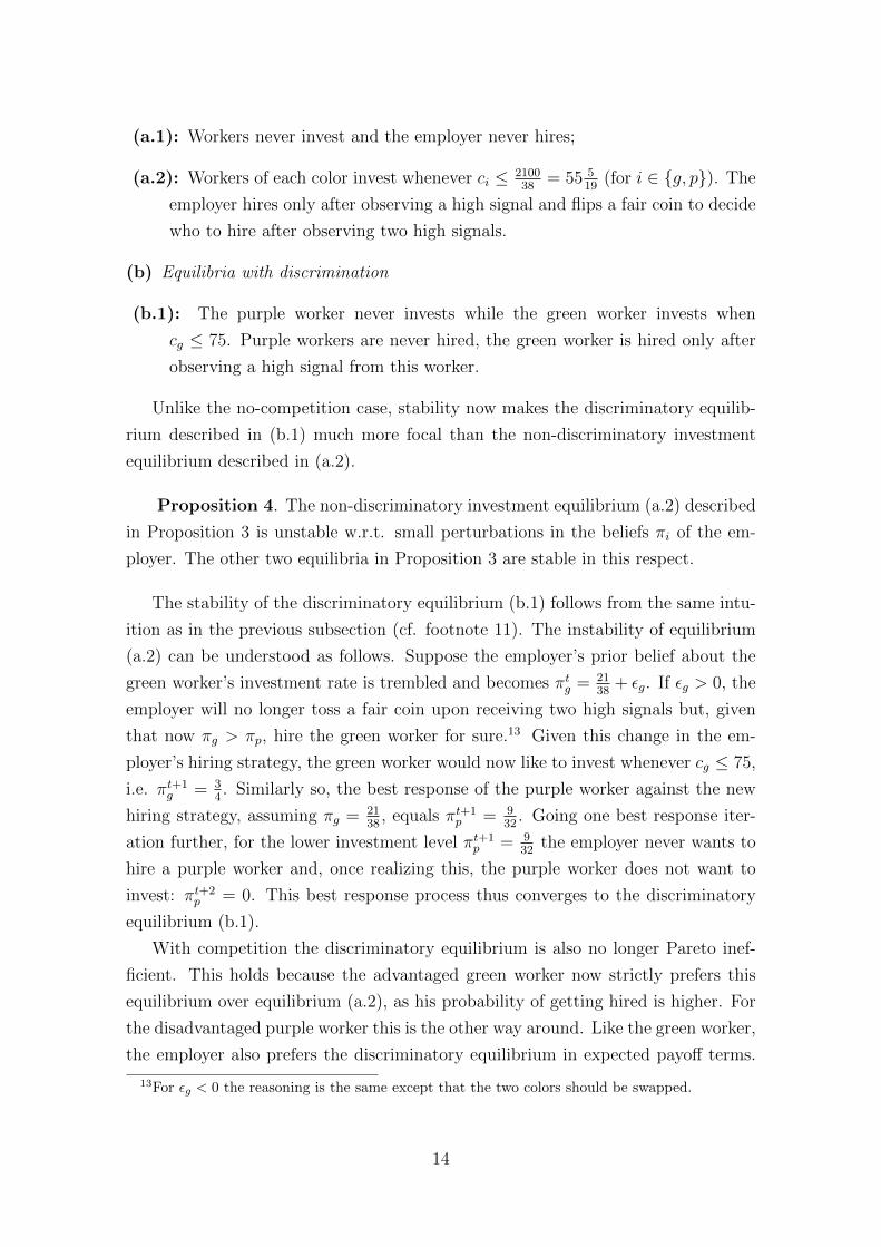
Unlike the no-competition case, stability now makes the discriminatory equilib-

rium described in (b.1) much more focal than the non-discriminatory investment

equilibrium described in (a.2).

Proposition 4. The non-discriminatory investment equilibrium (a.2) described

in Proposition 3 is unstable w.r.t. small perturbations in the beliefs πi of the em-

ployer. The other two equilibria in Proposition 3 are stable in this respect.

The stability of the discriminatory equilibrium (b.1) follows from the same intu-

ition as in the previous subsection (cf. footnote 11). The instability of equilibrium

(a.2) can be understood as follows. Suppose the employer’s prior belief about the

green worker’s investment rate is trembled and becomes πtg =

2138

+ εg. If εg > 0, the

employer will no longer toss a fair coin upon receiving two high signals but, given

that now πg > πp, hire the green worker for sure.13 Given this change in the em-

ployer’s hiring strategy, the green worker would now like to invest whenever cg ≤ 75,

i.e. πt+1g = 3

4. Similarly so, the best response of the purple worker against the new

hiring strategy, assuming πg = 2138, equals πt+1

p = 932. Going one best response iter-

ation further, for the lower investment level πt+1p = 9

32the employer never wants to

hire a purple worker and, once realizing this, the purple worker does not want to

invest: πt+2p = 0. This best response process thus converges to the discriminatory

equilibrium (b.1).

With competition the discriminatory equilibrium is also no longer Pareto inef-

ficient. This holds because the advantaged green worker now strictly prefers this

equilibrium over equilibrium (a.2), as his probability of getting hired is higher. For

the disadvantaged purple worker this is the other way around. Like the green worker,

the employer also prefers the discriminatory equilibrium in expected payoff terms.

13For εg < 0 the reasoning is the same except that the two colors should be swapped.

14

The intuition here is that, although the probability that a worker is hired is lower in

the discriminatory equilibrium, the expected quality of the hired worker is higher.

Summing up, both without and with competition a symmetric and an asym-

metric equilibrium with equilibrium investment exists. Without competition both

equilibria are stable and the symmetric equilibrium payoff dominates the asymmet-

ric one. But with competition only the asymmetric equilibrium is stable and this

equilibrium is also no longer payoff dominated. We therefore expect to observe

systematic discrimination only in the treatment with competition between workers.

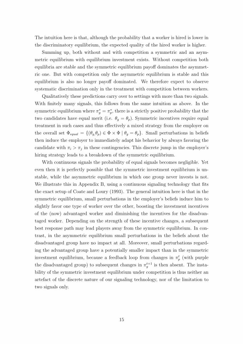
Qualitatively these predictions carry over to settings with more than two signals.

With finitely many signals, this follows from the same intuition as above. In the

symmetric equilibrium where π∗g = π∗

p, there is a strictly positive probability that the

two candidates have equal merit (i.e. θg = θp). Symmetric incentives require equal

treatment in such cases and thus effectively a mixed strategy from the employer on

the overall set Φequal = {(θg,θp) ∈ Φ× Φ | θg = θp}. Small perturbations in beliefs

then induce the employer to immediately adapt his behavior by always favoring the

candidate with πi > πj in these contingencies. This discrete jump in the employer’s

hiring strategy leads to a breakdown of the symmetric equilibrium.

With continuous signals the probability of equal signals becomes negligible. Yet

even then it is perfectly possible that the symmetric investment equilibrium is un-

stable, while the asymmetric equilibrium in which one group never invests is not.

We illustrate this in Appendix B, using a continuous signaling technology that fits

the exact setup of Coate and Loury (1993). The general intuition here is that in the

symmetric equilibrium, small perturbations in the employer’s beliefs induce him to

slightly favor one type of worker over the other, boosting the investment incentives

of the (now) advantaged worker and diminishing the incentives for the disadvan-

taged worker. Depending on the strength of these incentive changes, a subsequent

best response path may lead players away from the symmetric equilibrium. In con-

trast, in the asymmetric equilibrium small perturbations in the beliefs about the

disadvantaged group have no impact at all. Moreover, small perturbations regard-

ing the advantaged group have a potentially smaller impact than in the symmetric

investment equilibrium, because a feedback loop from changes in πtp (with purple

the disadvantaged group) to subsequent changes in πt+1g is then absent. The insta-

bility of the symmetric investment equilibrium under competition is thus neither an

artefact of the discrete nature of our signaling technology, nor of the limitation to

two signals only.

15

4 Experimental design and procedure

The computerized experiment was conducted at the CREED laboratory of the Uni-

versity of Amsterdam. Subjects were recruited from the student population in the

standard way. At the start of the experiment, subjects were randomly assigned ei-

ther the role of employer, green worker or purple worker. Subjects kept the same

role throughout the experiment. Subjects read the role-specific instructions on the

computer at their own pace and received a handout with a summary. The instruc-

tions provided context by using words like ‘employer’ and ‘worker’, but completely

avoided loaded terms like ‘discrimination’. Appendix C provides the instructions for

the experiment. All subjects had to answer some control questions testing their un-

derstanding of the instructions. The experiment would start only after each subject

successfully answered each question.

Each subject received a starting capital of 900 points. In addition, subjects

earned (or lost) money with their decisions in each period. At the end of the

experiment, points were exchanged for euros at the rate of 1 eurocent for each point.

The sessions lasted between one and two hours. A total of 144 subjects participated

in the experiment. The average earnings per subject were 30.10 euros (in a range of

14.80 euros to 47.00 euros). In every session, 1 or 2 matching-groups of 12 persons

were formed, each containing 4 employers, 4 green workers and 4 purple workers. In

each period, subjects were randomly rematched within their matching-group.

Each subject participated only once in one of the two treatments: ‘No Com-

petition’ and ‘Competition’. The only difference between the treatments was that

in Competition a purple and a green worker competed for the same job, while in

No Competition either a green or a purple worker was available for the job. In No

Competition, each employer was randomly matched to either a green or a purple

worker and the unmatched worker was inactive and had to wait for one period. In

Competition, each employer was randomly matched with one green and one purple

worker and both workers were active. Subjects were aware that they would never

be matched with the same person twice in a row.

In the experiment, the exact order of play as described in Section 3 was used.

At the start of each of the 50 periods, each active worker was informed of the

personal cost of investment. Costs differed across workers and periods. Each cost

was an independent draw from a uniform distribution, with every integer between 0

and 100 being equally likely. Then each active worker chose whether to ‘invest’ or

‘not invest’. After the active workers made their investment decisions, independent

signals were generated and sent to the employers. A signal could either be ‘high’

or ‘low’. If a worker decided to invest, the employer would receive a high signal

16

with probability 34and a low signal with probability 1

4. If a worker decided not

to invest, the employer would receive a high signal with probability 14and a low

signal with probability 34. The employer observed the signal but not the investment

decision itself. After observing the signal, the employer decided whether or not to

hire the given worker in No Competition, and whether to hire the green worker, the

purple worker, or none of the workers in Competition. The procedure to generate

the investment costs and the signaling technology were the same in both treatments.

At the end of the period, each subject received information about the investment

decisions of the active workers, the signal(s) received by the employer and the hiring

decision of the employer. A calculation of one’s own earnings for this period was

shown. Both treatments employed the payoffs listed in Figure 1. In No Competition,

workers who were inactive in a period received 10 points. At any moment, subjects

could observe their current cumulative earnings.

Figure 1: Payoffs used in the experimentEmployer

Hire Not Hire

WorkerInvest 160− c, 60 10− c, 20

Not Invest 160, −40 10, 20

Notes: Here c denotes the worker’s cost of investment.

In addition, subjects were continuously shown a social history screen that sum-

marized the decisions in the previous periods of the own matching-group. Workers

and employers observed a different history screen. The employers’ history screen

showed for each category ‘high signal’ and ‘low signal’ how often workers had cho-

sen to invest and not to invest. These numbers were given for each of the two colors

separately as well as for the pooled data. The workers’ history screen showed for

each decision ‘invest’ and ‘not invest’ how often a worker was and was not hired,

separately for each color and aggregated over the two colors. Examples of the history

screens are shown in Figure 2.

We provided subjects with a history screen because we wanted to facilitate their

strategic understanding of the game. Miller and Plott (1985) were the first to use a

similar social history (on black board) in a signaling experiment. They introduced it

in their later sessions to help subjects understand the relationship between types and

choices. Other papers have used role reversion to accomplish this goal. In signaling

games, after senders have become receivers, they do a better job in processing the

meaning of a signal (e.g., Brandts and Holt, 1992). Notice that in our experiment

especially the employers face a difficult task, because rational belief formation on

their part requires the use of Bayes’ rule. Gigerenzer and Hoffrage (1995) showed

17

Figure 2: Examples of social history screens of employers (above) and workers (be-low) based on hypothetical data

that subjects make much fewer errors against Bayes’ rule if they are presented with

natural frequencies like the ones they often encounter in real life. Given that our

experiment is not about testing the validity of Bayes’ rule in an abstract setting,

it made sense to provide a history screen that summarized the relevant natural

frequencies.14

5 Experimental results: Does competition trigger

discrimination?

Statistical discrimination arises when employers believe that one group of workers

invests more in their quality than another group. As a result, the disadvantaged

group is discouraged to invest which confirms the employers’ beliefs, even though the

groups started from ex-ante equal positions. For each matching-group of subjects, we

14Like the experiment of Fryer, Goeree and Holt (2005), our No Competition treatment is astraightforward implementation of the model of Coate and Loury (1993). There are some minordifferences between our experiments. For instance, Fryer et al. use different payoff parameters,they consider a setting where the signal has three levels (low, medium and high) instead of twoand in their experiment there are no inactive workers that we introduced to make No Competitioncomparable to Competition.

18

determined ex post which group was disadvantaged and which one was advantaged.

The criterion that we used was the average hiring probability after a high signal. If

over all 50 periods this probability was higher for the green group, then the green

group was labeled advantaged and if it was higher for the purple group, then the

purple group was labeled advantaged.

A consequence of this definition is that in each matching-group we have one ad-

vantaged and one disadvantaged group, even in cases where the hiring probabilities

differ only slightly.15 Our main hypothesis is that the difference in hiring proba-

bilities after a high signal between the advantaged and the disadvantaged group is

higher in Competition than in No Competition. In agreement with our conjecture

that we employed neutral colors, the green group turned out to be advantaged in 6

matching-groups while the purple group was advantaged in the other 6 cases.

In Section 3 we argued that small differences in investment behavior may have

profound implications for employers’ hiring behavior when workers from different

groups compete for the same job. Figure 3 displays the development of the average

investment decisions in the two treatments. In No Competition, the investments

for both the advantaged and disadvantaged group hover around 73%, not far away

from the 75% investment level predicted by the non-discrimination investment equi-

librium. Even though the advantaged group invests on average somewhat more than

the disadvantaged group, there are some periods where the investment levels of the

disadvantaged group surpass those of the advantaged group. In Competition, the

difference in investment levels is more pronounced and less capricious. A noticeable

difference in investment behavior arises approximately around period 10 after which

disadvantaged workers consistently invest less than advantaged workers.

15In fact, in two matching groups of No Competition we could not distinguish between the groupson the basis of this criterion because all workers were always hired after a high signal. In thesetwo cases we classified the groups on the basis of which group was more likely to be hired after alow signal.

19

Figure 3: Smoothed average investments across time�

0

0.2

0.4

0.6

0.8

1

1 6 11 16 21 26 31 36 41 46

period

investmentno

competition

invest advantaged invest disadvantaged

�

0

0.2

0.4

0.6

0.8

1

1 6 11 16 21 26 31 36 41 46

period

investmentcompetition


Notes: For each period, the average investment level in the interval [period -2, period+2] is displayed.

These observations are confirmed in Table 1, where we see that in the Competi-

tion treatment the modest difference in investment rates of the disadvantaged and

advantaged workers over all 50 periods is significant according to a Wilcoxon rank

test. Throughout this paper, unless we specify otherwise, we use a prudent testing

procedure in which independent averages per matching-group serve as data-points

(in each treatment, we have 6 matching-groups). The corresponding difference in

No Competition is not significant. The picture remains qualitatively the same when

we limit our attention to the final 25 periods.

Table 1: Investment decisions

Periods treatment disadvantaged invested advantaged invested Wilcoxon p (n=6)

1-50no competition 71.1% 74.1% 0.75

competition 50.8% 59.3% 0.03

26-50no competition 72.8% 72.2% 0.75

competition 51.8% 61.0% 0.06

Figure 4 shows how the workers’ investment decisions depend on their investment

costs. The figure suggests that subjects use a cutoff rule and invest if and only if

the cost level is sufficiently small. In agreement with the fact that in Competition

it is less lucrative to invest because two workers compete for one job only, we find

that subjects invest for a larger range of costs in No Competition.

20

Figure 4: Smoothed average investments as function of costs�

0

0.2

0.4

0.6

0.8

1

0 20 40 60 80 100

cost

investmentno

competition


�

0

0.2

0.4

0.6

0.8

1

0 20 40 60 80 100

cost

investmentcompetition


Notes: For each cost, the average investment levels for that cost in the interval [cost-2, cost+2] is displayed.

Our main result is illustrated in Figure 5. The figure shows how often advantaged

and disadvantaged workers were hired after sending a high signal over the different

periods, separately for No Competition and Competition. The hiring percentages of

advantaged and disadvantaged workers are practically identical in No Competition,

even though by construction the hiring percentages of the advantaged workers are

higher on average. Almost all workers are hired after a high signal, irrespective of

color. The picture is completely different for the competition treatment. Here, a

clear gap in hiring percentages emerges from the start of the experiment. This gap

is consistently sustained over the periods and seems to be growing.

21

Figure 5: Smoothed average of hiring after high signal across time�

0

0.2

0.4

0.6

0.8

1

1 6 11 16 21 26 31 36 41 46

period

hiring w orker high signal

nocompetition

hire advantaged hire disadvantaged

�

0

0.2

0.4

0.6

0.8

1

1 6 11 16 21 26 31 36 41 46

period

hiring w orker high signalcompetition

hire advantaged hire disadvantaged

Notes: For each period, the average hiring levels for that period in the interval [period-2, period+2] is displayed.

Table 2 summarizes the hiring behavior of the employers and confirms the picture

that emerges from Figure 5. Over all periods, the difference between the percentages

of advantaged and disadvantaged workers hired after a high signal is substantially

higher (25.8%) in Competition than in No Competition (3.1%). A Mann-Whitney

test comparing the differences in hiring rates rejects that they are equal across

treatments with p < 0.01. In Competition, discrimination of the disadvantaged

workers is underlined in the cases where both colors generate high signals. In those

cases the difference in hiring rates equals 40.6%.

If we look at the second half of the experiment only, the evidence for our conjec-

ture that statistical discrimination emerges when workers of different groups compete

for the same job is even more pronounced. Here, the difference in hiring rates after

a high signal equals 31.6% in Competition and 4.7% in No Competition, and the

difference in the differences is significant at p < 0.01. When both colors generate a

high signal in the latter part of the experiment, the difference in hiring rates grows

to 50.0%.16

16In agreement with theory, we do not find evidence of discrimination after a low signal. Workersare only occasionally hired after a low signal and the hiring rate does not depend on the color ofthe worker.

22

Table 2: Hiring decisionsPeriods signal treatment disadvantaged hired (1) advantaged hired (2) difference (2-1)

1-50

high no competition 96.1% 99.2% 3.1%

competition 52.3% 78.1% 25.8%

Mann-Whitney p (m=6;n=6) 0.004

low no competition 19.4% 27.1% 7.7%

competition 1.6% 4.8% 3.2%


2 high competition 25.6% 66.2% 40.6%

2 low competition 2.5% 8.5% 6.0%

26-50

high no competition 94.8% 99.5% 4.7%

competition 47.8% 79.4% 31.6%


low no competition 17.7% 31.1% 13.4%

competition 0.7% 4.8% 4.1%


2 high competition 19.4% 69.4% 50.0%

2 low competition 1.6% 9.4% 7.8%

Notes: The cells list the average hiring behavior by the employer conditional on the treatment and whether the

disadvantaged or advantaged worker emitted a low or a high signal (or in Competition, whether both workers

emitted a low or a high signal). The Mann-Whitney tests compare the difference between the treatments of the

differences in the employer’s hiring behavior of the advantaged and disadvantaged worker.

The dynamics in the data are well in line with the intuition provided by the stabil-

ity argument. In 4 of the 6 matching-groups in Competition, the group that initially

invested somewhat less than the other became already disadvantaged around period

10, and remained so throughout the entire experiment. In one matching-group,

the purple group of workers started investing a bit less in the first 5 periods and,

conditionally on a high signal, was also hired at a lower rate initially. Then the

purple group successfully boosted their investments and surpassed the green group

by period 10, after which they were consistently favored by the employers until the

end of the experiment. There was only one matching-group where it took longer

before the dust settled. In this group the green group started investing a bit more

and was favored in the first 20 periods, after which the purple group successfully

came back, invested more than green and was favored by the employers until the

end of the experiment.17 In contrast, the picture is much more random for No

Competition, where groups tended to be treated equally in the majority of cases. If

differences were made in how colors were treated, the advantage changed back and

17It seems that the dynamics were driven by accidental differences in initial behavior instead ofaccidental differences in initial cost draws. In the first ten periods, advantaged workers receivedan average cost of 50.4 (s.d. 29.4) while disadvantaged workers received an avarage cost draw of49.2 (s.d. 28.0). According to a Wilcoxon test, the difference is not significant (n=240, p=0.67).

23

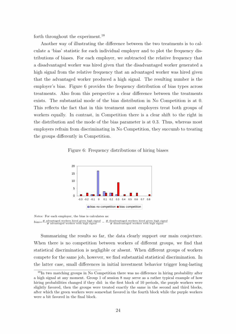
forth throughout the experiment.18

Another way of illustrating the difference between the two treatments is to cal-

culate a ‘bias’ statistic for each individual employer and to plot the frequency dis-

tributions of biases. For each employer, we subtracted the relative frequency that

a disadvantaged worker was hired given that the disadvantaged worker generated a

high signal from the relative frequency that an advantaged worker was hired given

that the advantaged worker produced a high signal. The resulting number is the

employer’s bias. Figure 6 provides the frequency distribution of bias types across

treatments. Also from this perspective a clear difference between the treatments

exists. The substantial mode of the bias distribution in No Competition is at 0.

This reflects the fact that in this treatment most employers treat both groups of

workers equally. In contrast, in Competition there is a clear shift to the right in

the distribution and the mode of the bias parameter is at 0.3. Thus, whereas most

employers refrain from discriminating in No Competition, they succumb to treating

the groups differently in Competition.

Figure 6: Frequency distributions of hiring biases�

0

5

10

15

20

-0.3 -0.2 -0.1 0 0.1 0.2 0.3 0.4 0.5 0.6 0.7 0.8

bias no competition bias competition

Notes: For each employer, the bias is calculates as:

bias=# advantaged workers hired given high signal# advantaged workers with high signal

− # disadvantaged workers hired given high signal# disadvantaged workers with high signal

Summarizing the results so far, the data clearly support our main conjecture.

When there is no competition between workers of different groups, we find that

statistical discrimination is negligible or absent. When different groups of workers

compete for the same job, however, we find substantial statistical discrimination. In

the latter case, small differences in initial investment behavior trigger long-lasting

18In two matching groups in No Competition there was no difference in hiring probability aftera high signal at any moment. Group 1 of session 8 may serve as a rather typical example of howhiring probabilities changed if they did: in the first block of 10 periods, the purple workers wereslightly favored, then the groups were treated exactly the same in the second and third blocks,after which the green workers were somewhat favored in the fourth block while the purple workerswere a bit favored in the final block.

24

statistical discrimination.

6 Color blind and discriminating employers

Although the results confirm our main hypothesis, the data do not accord with all

details of the theoretical analysis. The most striking difference is that disadvantaged

workers continue to invest at a fairly high level, even though theory suggests that

they should completely stop investing given that they are discriminated against. A

key ingredient of an explanation for this puzzle is that some of the employers in

Competition refrained from discriminating, despite being it in their best interest to

do so. Like Figure 6 already shows, there are some employers in Competition that

have biases close to 0. It thus appears that some of the employers completely ignore

investment differences between the two groups and continue hiring both colors at

an equal pace.

Based on our data we classify employers as being either ‘color blind’ or ‘discrim-

inating’ in the following way. For each employer in Competition, we conditioned on

the cases where the employer observed high signals from both workers and hired one

of them. If in such situations the employer hired the advantaged worker in at least

75% of the cases, the employer is considered to be discriminating. Otherwise he is

labelled color blind. Employing this definition, a substantial minority of 41.7% is

found to be color blind.19

In the presence of color blind employers, theoretical predictions regarding the

form statistical discrimination takes may change. To explore this, we analyze the

setup of Subsection 3.2 assuming that a fraction β (with 0 < β < 1) of the employers

is color blind. These employers use the following hiring strategy (with ρCB (θi; θj)

the probability that the color i worker is hired):

ρCB (θi; θj) =

1 if θi = θh and θj = θl

12

if θi = θj = θh

0 if θi = θl(6)

A color blind employer does not hire after observing two low signals, hires the worker

with the higher signal if signals differ and hires either worker with equal probability

in case of two high signals. Because a color blind employer ignores the workers’

investment strategies πi and πj, he does not necessarily best respond. The remaining

19One employer engaged in positive discrimination and hired disadvantaged workers significantlymore often than advantaged workers when both had high signals. Given that this was only onesubject, we decided to include this employer with the color blind employers.

25

fraction 1− β of discriminating employers does so, however, as they optimize their

expected payoffs (cf. expression (5)).

The characterization of equilibria for general values of β (and the other param-

eters in the model) is provided in Appendix A. Proposition 5 below does so for the

particular parameters used in the experiment and the fraction of β = 0.417 observed.

It focuses on the implications for the discriminatory equilibria.20

Proposition 5. The job market discrimination game with competition and

a fraction β = 0.417 of color blind employers allows the following discriminatory

equilibria:

(b.1): Overt discrimination equilibrium

The purple worker invests when cp ≤ 21.94, the green worker if cg ≤ 69.38. A

color blind employer uses hiring strategy (6). A discriminating employer never

hires the purple worker and hires the green worker only after observing a high

signal from this worker.

(b.2): Hidden discrimination equilibrium

The purple worker invests when cp ≤ 39.99, the green worker if cg ≤ 67.96. A

color blind employer uses hiring strategy (6). A discriminating employer hires

the purple worker after a high signal from this worker and a low signal from

the green worker and hires the green worker when observing a high signal from

this worker.

Equilibrium (b.1) in Proposition 5 corresponds to equilibrium (b.1) in Propo-

sition 3. Here a discriminating employer openly discriminates, because he ignores

purple workers altogether. Nevertheless, the presence of a fraction of color blind em-

ployers now induces the disadvantaged purple worker to invest with positive proba-

bility. Note that In the overt discrimination equilibrium, discriminating employers

are easily identified, because they refrain from hiring disadvantaged workers even

when these workers generate a higher signal.

Compared to Proposition 3, the presence of color blind employers opens up the

possibility that discrimination takes place in a hidden form. In equilibrium (b.2)

both types of employer hire the worker who generates the higher signal and different

treatment only occurs after two high signals.21 A discriminating employer then

20The presence of color blind employers does not affect the non-discriminatory equilibrium inwhich both workers invest (cf. equilibrium (a.2) in Proposition 3).

21To rationalize that the purple worker is hired by the discriminating employer if this workerhas the higher signal, equilibrium (b.2) requires a sufficiently high fraction β ≥ 0.181 of color

26

systematically hires the advantaged workers. Detecting this type of discrimination

is much harder. Only after a series of hiring observations where both workers have

equal merit, an outside observer will be able to distinguish a discriminating employer

from a color blind one.

To assess which type of discrimination fits our experimental data best, Table 3

reports the hiring decisions of the color blind and discriminating employers condi-

tional on the combination of signals observed.

Table 3: Actual hiring decisions and best responses in competition treatmentcolor blind employers (41.7%) discriminating employers (58.3%)

combination signals hire disadvantaged hire advantaged hire disadvantaged hire advantaged

both low 2.6% [0.0%] 9.5% [0.0%] 2.5% [0.6%] 8.1% [0.0%]

advantaged low,83.8% [97.1%] 1.0% [0.0%] 86.7% [88.5%] 0.6% [0.0%]

disadvantaged high

advantaged high,0.0% [0.0%] 85.5% [100.0%] 1.2% [0.0%] 96.3% [100.0%]

disadvantaged low

both high 42.0% [26.8%] 46.4% [73.2%] 12.5% [6.8%] 81.3% [92.7%]

Notes: The cells list the average actual hiring decisions. Between brackets best responses are displayed. Table is

based on periods 1-50.

It is not surprising that color blind employers hire the two types of workers with

approximately equal probability when both produce a high signal, in contrast to

the discriminating employers who favor the advantaged workers in such cases. This

result is a direct consequence of the classification procedure. Most interesting is how

discriminating employers behave when the disadvantaged worker generates a high

signal and the advantaged worker a low signal. The table shows that in such cases

discriminating employers overwhelmingly hire the disadvantaged worker. Thus, the

statistical discrimination observed in our experiment is best described by the hidden

discrimination equilibrium.

Table 3 also includes the best responses of the employers. When calculating these

statistics, we assumed that the employers’ beliefs coincided with what they observed

in the social history screen and that their hiring decisions maximized expected pay-

offs given these beliefs. Qualitatively, the actual employer decisions match the best

responses quite well, except for the case where color blind employers observed two

high signals. In those cases, they should have hired the advantaged workers much

more often than they did.

blind employers in order to exist. Similarly so, equilibrium (b.1) requires β ≤ 0.624 to rationalizethat the discriminating employer ignores purpe workers. For a large range of β-values these twoequilibria thus co-exist (obviously the π∗

i values in these equilibria vary with β, see Appendix A.3).Both equilibria are stable according to the stability criterion used in Section 2.

27

Table 4: Actual earnings and best response earnings employer in competition treat-ment (periods 1-50)

color blind employers (41.7%) discriminating employers (58.3%)

combination signals actual best response actual best response

both low 17.1 (18.5) 20.0 (0.0) 18.0 (17.1) 19.6 (4.7)

advantaged low,36.8 (37.8) 37.9 (40.8) 29.5 (42.7) 29.3 (43.1)

disadvantaged high

advantaged high,43.7 (32.0) 43.9 (36.9) 40.7 (38.8) 41.1 (39.3)

disadvantaged low

both high 38.0 (38.1) 42.6 (38.0) 37.7 (39.9) 37.9 (41.4)

Notes: The cells list the average actual hiring decisions. Standard deviations in parentheses. Table is based on

periods 1-50.

A natural question to ask is how costly it was for color blind employers to refrain

from discriminating after observing two high signals. Given that their behavior

stimulated disadvantaged workers to continue investing at a fairly high pace, it

turns out not to have been that costly. Table 4 shows the actual earnings of the

employers in comparison to the earnings that they would have received if they had

adhered to the best response model. Like in Table 3, the main discrepancy between

actual data and best responses occurs when color blind employers received two high

signals.22 In these cases employers earned roughly 10% less than they could have

done with optimal choices.23

In agreement with the hidden discrimination equilibrium, disadvantaged work-

ers continued investing at a high rate even while they were discriminated against.

Theoretically, the possibility to be matched with a color blind employer prevents the

unraveling of investments by disadvantaged workers. For the proportion of 41.7%

color blind employers in the experiment, the equilibrium investment rate of disad-

vantaged workers equals 40.0%. In the second part of the experiment, disadvantaged

workers invested at an even higher rate of 51.8%.24 Possibly, some disadvantaged

workers disliked being discriminated against, and fought back by investing somewhat

more than predicted. Nevertheless, the hidden discrimination equilibrium organizes

the main pattern observed in the data.

22The signaling process has a stochastic nature which means that some employers can be un-lucky by receiving relatively many high signals from workers who did not invest. To some extent,discriminating employers have been harmed by such randomness. Although their earnings are onaverage closer to their best response earnings, they do not earn more than color blind employers.

23The difference between actual and best response earnings when color blind employers face twohigh signals is weakly significant (Wilcoxon rank test, p = 0.07).

24In Competition, the difference between actual and equilibrium investments of disadvantagedworkers in the second part of the experiment is significant (Sign rank test, p=0.03).

28

7 Conclusion

In an experiment, we showed that competition between workers causes statistical

discrimination among originally equally skilled groups. When workers of different

groups compete for the same job, accidental differences in workers’ historical invest-

ment rates have profound effects on employers’ hiring behavior. In our experiment,

discrimination takes a hidden form. That is, a majority of the employers system-

atically favors workers of a particular group when they receive equal signals of the

applicants. In the other cases, they tend to hire the worker with the higher ranked

signal. This means that even the disadvantaged workers are relatively frequently

hired, which makes it harder to detect discrimination. This aspect may limit the

extent to which legal measures against discrimination can successfully be imple-

mented.

What are the welfare implications of our results? The Pareto efficiency criterion

is silent about which equilibrium (in the competition case) is better; the equilibria

facilitating discrimination and those without discrimination can not be ranked on

this criterion. From the perspective of overall surplus in society, one would rather

perversely conclude that when there is a scarcity of jobs, society is well served by

discrimination. This holds because discrimination may efficiently solve the coordi-

nation problem of who acquires costly education.25 When one group of workers is

ignored, the other group has higher incentives to invest in quality, which makes it

more attractive to hire workers from this group. The maximization of overall surplus

goes together with substantial social injustice, though. Therefore, when a group of

workers is discriminated, it is natural to consider affirmative action programs. We

do not doubt that affirmative action processes can diminish or perhaps even elimi-

nate discrimination in the labor market in the short term. There are good reasons

why affirmative action programs should not become permanent fixtures of the labor

market though. For instance, once the target is reached, it will be better to abandon

the program because affirmative action may dilute workers’ incentives to invest in

quality. An important implication suggested by our study is that the long run effec-

tiveness of affirmative action programs may ultimately depend on the presence or

25A similar conclusion is obtained by Norman (2003). He solves for the utilitarian social planner’soptimum in a version of the Coate and Loury model in which firms can employ workers in one of twojobs, either simple or complex. Only qualified workers are productive in the complex task, whilequalified and unqualified workers alike are equally productive in the simple task. Discriminationcan then help solving the matching problem of who should get the complex job, because fewermistakes are made in job assignment (as compared to the equal treatment case). The downsideis that workers from the disadvantaged group that could have invested more cheaply than themarginal worker from the advantaged group, remain unqualified. The same two forces operate inthe discriminatory equilibria of our competition setup.

29

absence of unemployment. Affirmative action programs may prove valuable without

unemployment, because our analysis suggests that discrimination does not easily

emerge from a situation where it is absent. However, in the presence of unemploy-

ment, once the target is reached and the affirmative action program is abandoned,

we would predict on the basis of our theory and experiments that discrimination

might soon again flourish once groups again start competing for the same jobs. In

such a situation, it may be better to first spend money on reducing unemployment

than to prematurely use it for affirmative action programs.

Appendix A

In this appendix we briefly elaborate on the characterization of equilibria for the

general case {r, w, P hq , P

hu , G(c)} (with r, w > 0 and P h

q > P hu ).

A.1 Setup without competition

With ρ∗ (πi, θsi) the probability of being hired after signal si, the color i worker

prefers to invest as long as ci ≤ w ·(P hq − P h

u

)·[ρ∗

(πi, θ

h)− ρ∗

(πi, θ

l)]. The r.h.s.

can be understood as follows.(P hq − P h

u

)gives the increase – due to investment –

in the probability that the color i worker generates a high signal. The term within

square brackets gives the increase in probability that the worker is hired if her

signal is high rather than low. Together, the product of these two terms gives the

increase in the probability that the worker is hired that is caused by investment.

Multiplied by the benefits w of getting the job this in turn gives the expected benefits

from investment. In equilibrium the color i worker invests as long as the costs of

investment do not exceed the expected benefits, hence:

π∗i = G

(w ·

(P hq − P h

u

)·[ρ∗

(πi, θ

h)− ρ∗

(πi, θ

l)])

(A.1)

From (4) and P hu < P h

q it follows that: (i) ρ∗(πi, θ

h)< 1 =⇒ ρ∗

(πi, θ

l)= 0 and (ii)

ρ∗(πi, θ

l)> 0 =⇒ ρ∗

(πi, θ

h)= 1. If the employer considers the worker marginally

capable at most after a high signal, he certainly thinks she is incapable after a low

signal. Similarly so, if the employer considers the worker already marginally suitable

at least when θi = θl, then he certainly thinks she is suitable after θi = θh. Based on

these two observations Proposition A.1 below characterizes the possible equilibria

that may exist. Recall that we assume throughout that the employer hires for sure

when indifferent, implying ρ∗ (πi, θsi) ∈ {0, 1} in the no competition case.

Proposition A.1. The job market discrimination game without competition

30

allows the following equilibria(π∗g , π

∗p

), with π∗

i for i = g, p independently taken

from:

(a) π∗i = 0. The employer never hires the color i worker. No further requirements

are needed;

(b) π∗i = G

(w ·

(P hq − P h

u

)). The employer only hires the color i worker if θi = θh.

To justify the employer’s hiring strategy it should hold that:(1− π∗

i

π∗i

)·(P hu

P hq

)≤ r ≤

(1− π∗

i

π∗i

)·(1− P h

u

1− P hq

)(A.2)

The parameters used in the experiment are such that condition (A.2) is satisfied for

π∗i = G

(w ·

(P hq − P h

u

))and thus equilibrium (b) exists. This is obviously not a

knife-edge case. To illustrate, let G(c) ' U [0, C] (for C > 0) and let w < C(Phq −Ph

u

) .The model then contains five parameters {r, w, P h

q , Phu , C}. For π∗

i = wC·(P hq − P h

u

)condition (A.2) becomes:[

1− wC·(P hq − P h

u

)wC·(P hq − P h

u

) ]·(P hu

P hq

)≤ r ≤

[1− w

C·(P hq − P h

u

)wC·(P hq − P h

u

) ]·(1− P h

u

1− P hq

)

From P hq > P h

u it follows that(

Phu

Phq

)<

(1−Ph

u

1−Phq

). For any given {w,P h

q , Ph

u, C} thus

a nonnegligible range of r-values exists for which condition (A.2) is satisfied. Given

the continuity of the l.h.s. and the r.h.s., this also holds for parameters that are

near {w,P h

q , Ph

u, C}.

A.2 Setup with competition

Assuming that the employer always hires one of the workers when indifferent

between hiring and not-hiring, the following general characterization can be given.

Proposition A.2. The job market discrimination game with competition allows



(a.1) π∗i = 0 for i = g, p. The employer never hires. No further requirements are

needed;

(a.2) π∗i = G(w ·

(P hq − P h

u

)· [(π∗i · P h

q + (1− π∗i ) · P h

u

)· 12+ (π∗

i ·(1− P h

q

)+ (1−

π∗i ) ·

(1− P h

u

))]) for i = g, p. The employer only hires a worker with θi = θh

31

and flips a fair coin if θg = θp = θh. To justify the employer’s hiring strategy

condition (A.2) should hold for i = g, p;

(a.3) π∗i = G

(w ·

(P hq − P h

u

)·[12

])for i = g, p. The employer always hires the

worker with the highest signal and flips a fair coin in case θg = θp. It should

hold that(

1−π∗i

π∗i

)·(

1−Phu

1−Phq

)≤ r for i = g, p;


(b.1) π∗g = G

(w ·

(P hq − P h

u

))and π∗

p = 0. The employer never hires a purple

worker, the green worker is hired iff θg = θh. For π∗i = π∗

g condition (A.2)

should hold;

(b.2) π∗g = G

(w ·

(P hq − P h

u

))and π∗

p = G(w ·(P hq − P h

u

)· [(π∗

g ·(1− P h

q

)+ (1−π∗

g) ·(1− P h

u

))]). The employer hires the purple worker iff θp = θh and θg = θl, and

hires the green worker iff θg = θh. For both π∗i = π∗

g and π∗i = π∗

p condition

(A.2) should hold;

(b.3) π∗g = G

(w ·

(P hq − P h

u

)·[π∗p · P h

q + (1− π∗p) · P h

u

])and π∗

p = G(w · (P hq −P h

u ) ·[π∗

g · (1 − P hq ) + (1 − π∗

g) ·(1− P h

u

)]). The employer hires the purple worker

iff θp = θh and θg = θl, and hires the green worker otherwise. For π∗i = π∗

g

it should hold that(

1−π∗i

π∗i

)·(

1−Phu

1−Phq

)≤ r and for π∗

i = π∗p it should hold that(

1−π∗i

π∗i

)·(

Phu

Phq

)≤ r. Moreover, π∗

g ≥ π∗p should hold.

The characterization of π∗i follows from a similar expression as in (A.1), where the

term within square brackets reflects the increase in the probability of getting hired

if θi = θh instead of θi = θl. Compared to Proposition 3 in the main text, the

possible equilibria (a.3), (b.2) and (b.3) are new. In the symmetric equilibrium

(a.3) the employer always hires a worker, even when two low signals are received.

The same applies for asymmetric equilibrium (b.3), but there the green worker is

favored in case of equal signals. These two equilibria cannot exist when condition

(A.2) is satisfied for π∗i = G

(w ·

(P hq − P h

u

)), i.e. when an equilibrium with positive

investment levels exists in the no-competition case.26

In asymmetric equilibrium (b.2) the employer does not hire when two low signals

are observed. The green worker invests more often than the purple one, so when two

high signals are observed the green worker is chosen. The purple worker is hired only

if θp = θh and θg = θl. Because condition (A.2) now has to be satisfied for both π∗g =

26Note that(

1−π∗i

π∗i

)·(

1−Phu

1−Phq

)is strictly decreasing in π∗

i . So, if r ≤(

1−π∗i

π∗i

)·(

1−Phu

1−Phq

)for

π∗i = G

(w ·

(Phq − Ph

u

)), we have r <

(1−π∗

i

π∗i

)·(

1−Phu

1−Phq

)for all π∗

i < G(w ·

(Phq − Ph

u

)). The

conditions in (a.3) and (b.3) thus cannot be satisfied at the same time.

32

G(w ·

(P hq − P h

u

))and π∗

p < G(w ·

(P hq − P h

u

)), this equilibrium only exists in a

strict subset of the cases for which equilibrium (b.1) exists. We chose our parameters

as to exclude this equilibrium. This has the advantage that only one symmetric and

one asymmetric equilibrium with investment co-exists. Both these equilibria have a

simple structure and are well apart. By excluding equilibrium (b.2) we also avoid

that our design is potentially biased in favor of observing discrimination. The issue

whether to coordinate on a non-discriminatory or discriminatory outcome is thus

particularly salient in our case.

A.3 Setup with competition and color blind employers

Assume that a fraction β (with 0 < β < 1) of the employers is color blind and

employs hiring strategy (6). Proposition A.3 below provides a general character-

ization of the discriminatory equilibria in that case, by describing the investment

behavior of the workers and the hiring strategy of the remaining fraction 1 − β of

discriminatory employers.

Proposition A.3. The job market discrimination game with competition and

a fraction β of color blind employers allows the following discriminatory equilibria:

(b.1) π∗g = G(w ·

(P hq − P h

u

)· [(1− β) + β · (1 − 1

2·(π∗p · P h

q +(1− π∗

p

)· P h

u

))])

and π∗p = G(w ·

(P hq − P h

u

)· [β · (1 − 1

2·(π∗g · P h

q +(1− π∗

g

)· P h

u

))]). The

discriminating employer never hires a purple worker and hires the green worker

iff θg = θh. For π∗i = π∗

g condition (A.2) should hold and for π∗i = π∗

p it should

hold that r ≤(

1−π∗i

π∗i

)·(

Phu

Phq

);

(b.2) π∗g = G(w ·

(P hq − P h

u

)· [(1− β) + β · (1− 1

2·(π∗p · P h

q +(1− π∗

p

)· P h

u

))]) and

π∗p = G(w ·

(P hq − P h

u

)· [(1− β) ·

(π∗g ·

(1− P h

q

)+(1− π∗

g

)·(1− P h

u

))+β ·(1−

12·(π∗g · P h

q +(1− π∗

g

)· P h

u

))]). The discriminating employer hires the purple

worker iff θp = θh and θg = θl, and hires the green worker iff θg = θh. For both

π∗i = π∗

g and π∗i = π∗

p condition (A.2) should hold;

(b.3) π∗g = G(w ·

(P hq − P h

u

)· [(1 − β) · (π∗

p · P hq + (1 − π∗

p) · P hu ) + β · (1 − 1

2·(

π∗p · P h

q +(1− π∗

p

)· P h

u

))]) and π∗

p = G(w·(P hq − P h

u

)·[(1− β)·(π∗

g ·(1− P h

q

)+(

1− π∗g

)·(1−P h

u ))+β ·(1− 12·(π∗g · P h

q +(1− π∗

g

)· P h

u

))]). The discriminating

employer hires the purple worker iff θp = θh and θg = θl, and hires the green

worker otherwise. For π∗i = π∗

g it should hold that(

1−π∗i

π∗i

)·(

1−Phu

1−Phq

)≤ r and

for π∗i = π∗

p it should hold that(

1−π∗i

π∗i

)·(

Phu

Phq

)≤ r. Moreover, π∗

g ≥ π∗p should

hold.

33

The characterization of workers’ investment behavior again follows from a similar

expression as in (A.1), where the term within square brackets reflects the increase in

the probability of getting hired if θi = θh instead of θi = θl. This term now consists

of two elements. With probability 1− β the worker faces a discriminating employer

and the probability of getting hired after θi = θh instead of θi = θl equals the one as

in Proposition A.2 for the corresponding case (this explains why we use the labels

(b.1) through (b.3) in Proposition A.3 as well). With probability β, worker i faces a

color blind employer and the increase in the probability of getting hired after θi = θh

instead of θi = θl equals (1− 12·(π∗j · P h

q +(1− π∗

j

)· P h

u

)). The latter follows because

with probability(π∗j · P h

q +(1− π∗

j

)· P h

u

)the competitor j generates a high signal

as well and the employer then chooses each worker with equal probabilities. The

overall term is simply the probability weighted average of the two elements.

Just as in the absence of color blind employers (cf. Appendix A.2), equilibrium

(b.3) does not exist when condition (A.2) is satisfied for π∗i = G(w · (P h

q − P hu )).

This is the case considered in the experiment. Equilibrium (b.1) only exists when

the fraction of color blind employers β is not too large. This holds because π∗p

should be sufficiently low such that never hiring the purple worker is indeed a best

response for the discriminating employer. For the parameters used in the experiment

{r, w, P hq , P

hu , G(c)} =

{23, 150, 3

4, 14, U [0, 100]

}it should hold that π∗

p ≤ 13, which is

the case for β ≤ 0.624.27 In a similar vein, in equilibrium (b.2) the discriminating

employer should be willing to hiring the purple worker after θp = θh, i.e. π∗p ≥ 1

3

is needed. This requires a sufficiently high fraction of color blind employers β ≥0.181.28 Therefore, for 0.181 ≤ β ≤ 0.624 the two types of equilibria co-exist.

Appendix B

We consider the setup with competition using a continuous signaling technology.

Assume that θi ∈ [0, 1] and let Fq (θ) = θk (for k > 1) be the probability distribution

of θ in case the worker is qualified and Fu (θ) = θ if she is unqualified. Parameter

k reflects the accuracy of the signaling technology; the higher k, the more likely

27For the parameters used in the experiment the equilibrium level of π∗p in equilibrium (b.1)

equals:

π∗p =

114 β + 3

32β2

163 − 3

16β2

28For the parameters used in the experiment the equilibrium level of π∗p in equilibrium (b.2)

equals:

π∗p =

(34 + 1

8β)− 3

8

(1− 1

2β) (

1− 18β

)43 − 3

32

(1− 1

2β)β

34

Table 5: Overview of asymmetric and symmetric equilibriaπ∗g = π∗ > 0 and π∗

p = 0 π∗g = π∗

p = π∗ > 0k π∗

Low π∗High π∗

Low π∗High

2 − − − −3 0.444 0.575S − −4 0.331 0.689S 0.343 0.5345 0.270 0.756S 0.274 0.5966 0.229 0.805S 0.230 0.6357 0.199 0.842S 0.200 0.6648 0.176 0.873S 0.176 0.6869 0.157 0.897 0.158 0.70310 0.142 0.917 0.143 0.71720 0.073 0.995 0.073 0.783Notes: Based on parameters used in experiment: γ = 3

2and r = 2

3. Only those equilibria with superscript S are

stable.

it is that a qualified worker generates a high signal. We also assume that G(c) 'U [0, 1

γw], with γ > 0 (and w > 0 the worker’s wage).

For the above family of signaling technologies the following features can be shown

analytically.29 For low levels of k no equilibria with positive investment levels exist.

The threshold value of k for which an asymmetric equilibrium with π∗g = π∗ > 0

and π∗p = 0 exists is lower than the threshold for a symmetric equilibrium (with

π∗g = π∗

p = π∗ > 0) to exist. If an equilibrium of a particular type exists, genericalIy

two such equilibria exist side by side: i.e. π∗ = π∗Low and π∗ = π∗

High. The one based

on π∗ = π∗Low is necessarily unstable.

We have no analytical result establishing the stability of the other asymmetric

equilibrium. Instead, for the parameters used in the experiment, we verify the

stability of the equilibrium based on π∗High by numerically calculating the relevant

Jacobian.30 We do so for various levels of k, see Table 5 Only equilibria with a

superscript S are stable.

If the signal is very noisy (low k), it is too difficult for a qualified worker to

convince the employer that she is worth hiring and no equilibrium with positive

investments exists. For higher values of k the employer is more easily convinced

in case a high signal is observed. Asymmetric equilibria exist for a larger range

29See the extended online version of this appendix available at: http://www.creedexperi-ment.nl/publications/papers.php.

30Equilibrium investments are characterized as the solutions (π∗g , π

∗p) to a system of two equations

similar to (A.1): πg = Gg(πg, πp) and πp = Gp(πp, πg). Stability follows from evaluating the

Jacobian matrix (based on∂Gi(πi,πj)

∂πj) in the point (π∗

g , π∗p). If both eigenvalues are below one in

absolute value, the equilibrium is stable.

35

of k-values than symmetric equilibria do. The asymmetric equilibrium based on

π∗ = π∗High is stable for intermediate k-values, while for the symmetric equilibrium

this is not the case. Hence for a nonnegligible range of k-values asymmetric and

symmetric equilibria both exist, but only the asymmetric equilibrium (based on

π∗High) is stable. In terms of equilibrium investment levels, the case of k = 5 comes

closest to the discrete setup considered in the experiment (with respectively π∗ =

0.750 and π∗ = 0.553); this case belongs to the relevant range.

Appendix C (Not for publication)

This appendix contains the instructions used in the Competition treatment of the

experiment, both for employers are for workers. The instructions used in the No

Competition treatment are similar.

Instructions for employers in Competition

Welcome to this experiment on decision-making. Please read the following instruc-

tions carefully. As soon as everyone has finished reading the instructions you will

receive a handout with a summary. During the experiment you will be asked to

make a number of decisions. Your decisions and those of other participants will

determine your earnings. At the start of the experiment you will receive a starting

capital of 900 points. In addition you will earn money with your decisions. The

experiment consists of 50 rounds. During the experiment, your earnings will be

denoted in points. Your earnings in the experiment equal the sum of the starting

capital and your earnings in the 50 rounds. At the end of the experiment, your

earnings in points will be transferred into money. For each point you earn, you will

receive 1 euro cent. Hence, 100 points are equal to 1 euro. Your earnings will be

privately paid to you in cash.

ROLES

Some participants have the role of EMPLOYER, some participants perform the

role of PURPLE WORKER and some have the role of GREEN WORKER. In all

50 rounds you keep the same role and, if you are a worker, the same color.

Your role is: EMPLOYER

DECISIONS

In each round, each employer is matched with a GREEN and a PURPLE worker.

The employer decides to hire either nobody, the green worker or the purple worker.

36

The employer thus cannot hire both workers at the same time. The employer re-

ceives a positive payoff if s/he hires a worker who invested in her/his productivity,

but receives a negative payoff if s/he hires a worker who did not invest in her/his

productivity. If the employer hires nobody, s/he receives a small positive payoff. A

worker earns a positive payoff if s/he is hired. If a worker is not hired, s/he earns

a small positive payoff. S/He incurs a COST if s/he invests in her/his productivity,

independently of whether or not s/he is hired. At the time the employer has to

make the hiring decision, s/he is not informed about the investment decisions of the

two workers. Instead, s/he receives a signal of the green worker and a signal of the

purple worker that corresponds to the investment decisions of these workers in the

following way.

If the worker invested, her/his signal is HIGH with probability 75% and it is

LOW with probability 25%. If the worker did not invest, her/his signal is HIGH

with probability 25% and it is LOW with probability 75%. So the signal is often

but not always in agreement with the investment decision. The worker’s probability

that a signal is high or low does not depend on any other worker’s probability that

her/his signal was high or low. Also, the probability that a worker’s signal is high

or low is independent of decisions made by the worker in any previous round.

At the start of a round, each worker is informed of the own COST of investing.

This cost will be a random number between 0 and 100 points. Each of these numbers

is equally likely. In each round, every worker is assigned a new (and independent)

cost level. Therefore, the different workers (most likely) have different costs in a

round, and the same worker (most likely) has different costs across rounds.

PAYOFFS

The workers’ investment decisions and the employer’s hiring decision lead to the

following payoffs:

(i) Payoff employer after hiring = 60 if hired worker invested.

(ii) Payoff employer after hiring = -40 if hired worker did not invest.

(iii) Payoff employer after not hiring = 20 (independent of workers’ investment

decisions).

(iv) Payoff worker after investing = 160 – cost if hired by employer.

(v) Payoff worker after investing = 10 – cost if not hired by employer.

37

(vi) Payoff worker after not investing = 160 if hired by employer.

(vii) Payoff worker after not investing = 10 if not hired by employer.

Notice that there are no differences in the rules for green and purple workers. In

particular, there are no differences in the green worker’s and purple worker’s prob-

abilities of good and bad signals. Also, the cost of investing is determined with the

same procedure for the two groups of workers and the payoffs are also determined

in exactly the same way.

SEQUENCE OF EVENTS

Summarizing, each round is characterized by the following sequence of events:

1. The workers are privately informed of the own cost of investment.

2. Each worker decides whether or not to invest.

3. The employer observes a high or low signal for each worker, but not the work-

ers’ investment decisions.

4. The employer decides to hire nobody, the green worker or the purple worker.

Then employer and workers receive payoffs based on the choices made.

MATCHING PROCEDURE

In each round, each employer will be randomly matched to another green worker

and another purple worker. You will never learn with whom you are matched. The

random matching scheme is chosen such that three participants will never be coupled

again in two subsequent rounds.

INFORMATION END OF ROUND

At the end of a round, each participant will be informed of the choices of the

participants with whom s/he is matched and the own payoff.

HISTORY OVERVIEW

The lower part of the screen provides an overview of the results of all rounds

already completed. Apart from your own results in the previous rounds, the history

overview also contains the results of 3 other employers. In total, you are thus

informed about the past results of the same group of 4 employers (one of which is

yourself) and 8 workers. Below you see an example of the history overview (with

arbitrary numbers).

38

The upper part of the history overview shows what happened in the cases where

employers received a HIGH signal. The row INVEST lists the number of cases in

which the worker’s signal was HIGH after investing. The row NOT INVEST lists

the number of cases in which the worker’s signal was HIGH after not investing.

In the first purple column, the results for only the purple workers are listed and

in the second green column the results for only the green workers are listed. In

the final column the results of the two groups of workers are combined. In each

cell, after the number the corresponding percentage is listed. The lower part of the

history overview summarizes the previous choices of workers whose signal was LOW.

(Workers observe a history overview that is organized in another way: they observe

the number of times purple, green and combined workers are hired, separated for

having made an investment or not.)

Instructions for workers in Competition

Welcome to this experiment on decision-making. Please read the following instruc-

tions carefully. As soon as everyone has finished reading the instructions you will

receive a handout with a summary. During the experiment you will be asked to

make a number of decisions. Your decisions and those of other participants will

determine your earnings. At the start of the experiment you will receive a starting

capital of 900 points. In addition you will earn money with your decisions. The

experiment consists of 50 rounds. During the experiment, your earnings will be

denoted in points. Your earnings in the experiment equal the sum of the starting

capital and your earnings in the 50 rounds. At the end of the experiment, your

earnings in points will be transferred into money. For each point you earn, you will

receive 1 euro cent. Hence, 100 points are equal to 1 euro. Your earnings will be

privately paid to you in cash.

ROLES

39

Some participants have the role of EMPLOYER, some participants perform the

role of PURPLE WORKER and some have the role of GREEN WORKER. In all

50 rounds you keep the same role and, if you are a worker, the same color.

Your role is: WORKER

You will learn at the start of the experiment whether you are a green or purple

worker.

DECISIONS

In each round, each employer is matched with a GREEN and a PURPLE worker.

The employer decides to hire either nobody, the green worker or the purple worker.

The employer thus cannot hire both workers at the same time. The employer re-

ceives a positive payoff if s/he hires a worker who invested in her/his productivity,

but receives a negative payoff if s/he hires a worker who did not invest in her/his

productivity. If the employer hires nobody, s/he receives a small positive payoff. A

worker earns a positive payoff if s/he is hired. If a worker is not hired, s/he earns

a small positive payoff. S/He incurs a COST if s/he invests in her/his productivity,

independently of whether or not s/he is hired. At the time the employer has to

make the hiring decision, s/he is not informed about the investment decisions of the

two workers. Instead, s/he receives a signal of the green worker and a signal of the

purple worker that corresponds to the investment decisions of these workers in the

following way.

If the worker invested, her/his signal is HIGH with probability 75% and it is

LOW with probability 25%. If the worker did not invest, her/his signal is HIGH

with probability 25% and it is LOW with probability 75%. So the signal is often

but not always in agreement with the investment decision. The worker’s probability

that a signal is high or low does not depend on any other worker’s probability that

her/his signal was high or low. Also, the probability that a worker’s signal is high

or low is independent of decisions made by the worker in any previous round.

At the start of a round, each worker is informed of the own COST of investing.

This cost will be a random number between 0 and 100 points. Each of these numbers

is equally likely. In each round, every worker is assigned a new (and independent)

cost level. Therefore, the different workers (most likely) have different costs in a

round, and the same worker (most likely) has different costs across rounds.

PAYOFFS

The workers’ investment decisions and the employer’s hiring decision lead to the

following payoffs:

40

(i) Payoff employer after hiring = 60 if hired worker invested.

(ii) Payoff employer after hiring = -40 if hired worker did not invest.

(iii) Payoff employer after not hiring = 20 (independent of workers’ investment

decisions).

(iv) Payoff worker after investing = 160 – cost if hired by employer.

(v) Payoff worker after investing = 10 – cost if not hired by employer.

(vi) Payoff worker after not investing = 160 if hired by employer.

(vii) Payoff worker after not investing = 10 if not hired by employer.

Notice that there are no differences in the rules for green and purple workers. In

particular, there are no differences in the green worker’s and purple worker’s prob-

abilities of good and bad signals. Also, the cost of investing is determined with the

same procedure for the two groups of workers and the payoffs are also determined

in exactly the same way.

SEQUENCE OF EVENTS

Summarizing, each round is characterized by the following sequence of events:

1. The workers are privately informed of the own cost of investment.

2. Each worker decides whether or not to invest.

3. The employer observes a high or low signal for each worker, but not the work-

ers’ investment decisions.

4. The employer decides to hire nobody, the green worker or the purple worker.

Then employer and workers receive payoffs based on the choices made.

MATCHING PROCEDURE

In each round, each employer will be randomly matched to another green worker

and another purple worker. You will never learn with whom you are matched. The

random matching scheme is chosen such that three participants will never be coupled

again in two subsequent rounds.

INFORMATION END OF ROUND

41

At the end of a round, each participant will be informed of the choices of the

participants with whom s/he is matched and the own payoff.

HISTORY OVERVIEW

The lower part of the screen provides an overview of the results of all rounds

already completed. Apart from your own results in the previous rounds, the history

overview also contains the results of 7 other workers. In total, you are thus informed

about the past results of the same group of 8 workers (one of which is yourself) and

4 employers. Below you see an example of the history overview (with arbitrary

numbers).

The upper part of the history overview shows what happened in the cases where

workers chose to INVEST. The row HIRED lists the number of cases in which the

employer decided to hire a worker after investing. The row NOT HIRED lists the

number of cases in which the employer decided to not hire a worker after investing.

In the first purple column, the results for only the purple workers are listed and in

the second green column the results for only the green workers are listed. In the final

column the results of the two groups of workers are combined. In each cell, after

the number the corresponding percentage is listed. The lower part of the history

overview summarizes the previous choices of employers after a worker did not invest

in exactly the same way. (Employers observe a history overview that is organized

in another way: they observe the number of investments and non investments of

purple, green and combined workers, separated for the signal being high and the

signal being low).

42

References

[1] Abbink, K., J. Brandts, B. Hermann and H. Orzen, 2010: “Intergroup Conflict

and Intra-Group Punishment in an Experimental Contest Game”, American

Economic Review 100, 420-447.

[2] Altonji, J.G. and R.M. Blank, 1999: “Race and Gender in the Labor Market”.

In Handbook of Labor Economics, Vol 3C, ed. Ashenfelter, O. and D. Card.

Amsterdam: North Holland.

[3] Akerlof, G.A., and R.E. Kranton, 2010: Identity Economics. Princeton: Prince-

ton University Press.

[4] Andreoni, J. and R. Petrie, 2008: “Beauty, Gender and Stereotypes: Evidence

from Laboratory Experiments”, Journal of Economic Psychology 29, 73-93.

[5] Anderson, L.R., R.G. Fryer and C.A. Holt, 2007: “Experimental Studies of Dis-

crimination”, in the Handbook of Economics of Discrimination, ed. W. Rogers,

97-118. Massachusetts: Edward Elgar Publishers.

[6] Arrow, K.J., 1971: “Some Models of Racial Discrimination in the Labor Mar-

ket”, Rand Corporation, RM-5253-RC.

[7] Arrow, K.J., 1973: “The Theory of Discrimination”, in Discrimination in La-

bor Markets, eds. O. Ashenfelter and A. Rees, 3-33. Princeton NJ: Princeton

University Press.

[8] Arulampam, W., A.L. Booth and M.L. Bryan, 2007: “Is there a Glass Ceiling

over Europe? Exploring the Gender Pay Gap across the Wages Distribution”,

Industrial and Labor Relations Review 60, 163-186.

[9] Azmat, G., M. Guell and A. Manning, 2006: “Gender Gaps in Unemployment

Rates in OECD Countries”, Journal of Labor Economics 24, 1-37.

[10] Balafoutas, L. and M. Sutter, 2012: “Affirmative Action Policies Promote

Women and Do Not Harm Efficiency in the Laboratory”, Science 335, 579-582.

[11] Becker, G.S., 1971: The Economics of Discrimination. Second Edition.

Chicago: University of Chicago Press.

[12] Bertrand, M. and S. Mullainathan, 2004: “Are Emily and Greg More Em-

ployable Than Lakisha and Jamal? A Field Experiment on Labor Market

Discrimination”, American Economic Review 94, 991-1013.

43

[13] Blau, F.D. and L.M. Kahn, 1992: “The Gender Earnings Gap: Learning from

International Comparisons”, American Economic Review 82, 533-538.

[14] Blau, F.D. and L.M. Kahn, 2003: “Understanding International Differences in

the Gender Pay Gap”, Journal of Labor Economics 21, 106-144.

[15] Brandts, J., and C. A. Holt, 1992: “An Experimental Test of Equilibrium

Dominance in Signaling Games”, American Economic Review, 82, 1350-1365.

[16] Calsamiglia, C., J. Franke and P. Rey-Biel, 2011: “The Incentive Effects of

Affirmative Action in a Real Effort Tournament”, Working Paper.

[17] CBS, 2010: Werkloosheid naar herkomst. http://www.cbs.nl/nl-NL/menu/the-

mas/arbeid-sociale-zekerheid/publicaties/arbeidsmarkt-vogelvlucht/structuur-

arbeidsmarkt/2006-arbeidsmarkt-vv-werkl-herkomst-art.htm.

[18] Charness, G. and P. Kuhn, 2010: “Lab Labor: What Can Labor Economists

Learn from the Lab?” Manuscript prepared for Handbook of Labor Economics

vol. 4, eds. O. Ashenfelter and D. Card.

[19] Charness, G., L. Rigotti, and A. Rustichini, 2007: “Individual Behavior and

Group Membership”, American Economic Review 97, 1340-1352.

[20] Chaudhuri, S. and R. Sethi, 2008: “Statistical Discrimination with Peer Ef-

fects: Can Integration Eliminate Negative Stereotypes?”, Review of Economic

Studies, 75, 579-596.

[21] Chen, Y. and S.X. Li, 2009: “Group Identity and Social Preferences”, American


[22] Coate, S. and G. Loury, 1993: “Will Affirmative Action Eliminate Negative

Stereotypes?”, American Economic Review 83, 1220-1240.

[23] Corns, A. and A. Schotter, 1999: “Can Affirmative Action Be Cost Effective?

An Experimental Examination of Price Preference Auctions”, American Eco-

nomic Review 89, 291-305.

[24] Darity, W. A, and P.L. Mason, 1998: “Evidence on Discrimination in Employ-

ment: Codes of Color, Codes of Gender”, Journal of Economic Perspectives 12,

63-90.

[25] Farmer, A. and D. Terrell, 1996: “Discrimination, Bayesian Updating of Em-

ployers’ Beliefs, and Human Capital Accumulation”, Economic Inquiry 34,

204-219.

44

[26] Feltovich, N. and C. Papageorgiou, 2004: “An experimental Study of Statistical

Discrimination by Employers”, Southern Economic Journal 70, 837-849.

[27] Feltovich, N., Gangadharan, L. and M.P. Kidd, 2011: “Must Positive Discrimi-

nation be Permanent? The Impact of Implementing and Removing Affirmative-

Action Programs on Workers’ Skill Acquisition”, Working Paper.

[28] Fershtman, C. and U. Gneezy, 2001: “Discrimination in a Segmented Society:

An Experimental Approach”, Quarterly Journal of Economics 116, 351-377.

[29] Fershtman, C., U. Gneezy and F. Verboven, 2005: “Discrimination and Nepo-

tism: The Efficiency of the Anonimity Rule”, Journal of Legal Studies 34,

371-396.

[30] Fryer, R.G.., J.K. Goeree and C.A. Holt, 2005: “Classroom Games: Experience-

Based Discrimination”, Journal of Economic Education 36, 160-170.

[31] Fryer, R.G., S.D. Levitt and J.A. List, 2008: “Exploring the Impact of Financial

Incentives on Stereotype Threat: Evidence from a Pilot Experiment”, American


[32] Fryer, R.G. and G.C. Loury, 2005: “Affirmative Action in Winner-Take-All

Markets”, Journal of Economic Inequality 3, 263-280.

[33] Gigerenzer, G. and U. Hoffrage, 1995: “How to Improve Bayesian Reasoning

without Instructions: Frequency Formats”, Psychological Review, 102, 684-704.

[34] Gneezy, U., M. Niederle and A. Rustichini, 2003: “Performance in Competi-

tive Environments: Gender Differences”, Quarterly Journal of Economics 118,

1049-1074.

[35] Gneezy, U., J. List and M.K. Price, 2012: “Toward an Understanding of why

People Discriminate: Evidence from a Series of Natural Field Experiments”,

NBER Working Paper Series, no. 17855.

[36] Goette, L., D. Huffman, S. Meier and M. Sutter, 2010: “Group Membership,

Competition and Altruistic Versus Antisocial Punishment: Evidence from Ran-

domly Assigned Army Groups”, Discussion Paper, IZA DP No. 5189.

[37] Goldin, C., and C. Rouse, 2000: “Orchestrating Impartiality: The Impact

of “Blind” Auditions on Female Musicians”, American Economic Review 90,

715-741.

45

[38] Hargreaves Heap, S.P. and D.J. Zizzo, 2009: “The Value of Groups”, American


[39] Kidd, M.P., P.S. Carlin and J. Pot, 2008: “Experimenting with Affirmative

Action: The Coate and Loury Model”, The Economic Record 84, 322-337.

[40] List, J.A., 2004: “The Nature and Extent of Discrimination in the Marketplace:

Evidence from the Field”, Quarterly Journal of Economics 119, 49-89.

[41] Mailath, G.J., L. Samuelson, and A. Shaked, 2000: “Endogenous Inequality in

Integrated Labor Markets with Two-Sided Search”, American Economic Review

90, 46-72.

[42] Moro, A., and P. Norman, 2004: “A General Equilibrium Model of Statistical

Discrimination”, Journal of Economic Theory 114, 1-30.

[43] Miller, R.M. and C.R. Plott, 1985: “Product Quality Signaling in Experimental

Markets”, Econometrica, 53, 837-872.

[44] Niederle, M., C. Segal and L. Vesterlund, 2008: “How Costly is Diversity?

Affirmative Action in Light of Gender Differences in Competitiveness”, NBER

Discussion Paper.

[45] Norman, P., 2003: “Statistical Discrimination and Efficiency”, Review of Eco-

nomic Studies, 70, 615-627.

[46] Phelps, E.S., 1972: “The Statistical Theory of Racism and Sexism”, American


[47] Reuben, E., P. Sapienza and L. Zingales, 2010: “The Glass Ceiling in Experi-

mental Markets”, Discussion Paper, Columbia University.

[48] Riach, P.A. and J. Rich, 2002: “Field Experiments of Discrimination in the

Market Place”, Economic Journal 112, 480-518.

[49] Schotter, A., and K. Weigelt, 1992: “Asymmetric Tournaments, Equal Oppor-

tunity Laws, and Affirmative Action: Some Experimental Results”, Quarterly

Journal of Economics 107, 511-539.

[50] Sherif, M., O.J. Harvey, B.J. White, W.R. Hood, and C. W. Sherif, 1954:

Intergroup Conflict and Cooperation: The Robbers Cave Experiment. Norman,

OK: University Book Exchange.

46

[51] Tajfel, H., M.G. Billig, R.P. Bundy, and C. Flament, 1971: “Social Catego-

rization and Intergroup Behavior”, European Journal of Social Psychology 1,

149-178.

[52] Yoo, S.H., 2010: “A Theory on Group Inequality: the Nature of Conflict”,

Discussion Paper, Nanyang Technological University.

[53] Zizzo, D.J., 2011: “You are not in my Boat: Common Fate and Discrimination

against Outgroup Members”, International Review of Economics 58, 91-103.

47

Date post:	11-Mar-2020
Category:	Documents
Upload:	others
View:	2 times
Download:	0 times

Discrimination in the Labor Market: The Curse of ...Discrimination in the Labor Market: The Curse of...

Documents