Dissertation Paper Real effective exchange rates and their influence on Romania’s trade with...

Dissertation Paper

Real effective exchange rates and their influence on Romania’s trade with European Union Countries

MSc Student :Grigorescu Madalina

Supervisor : Professor Moisa Altar

ACADEMY OF ECONOMIC STUDIES, BUCHARESTDOCTORAL SCHOOL OF FINANCE AND BANKING

DOFIN

Topics

Objectives Introduction Review of the literature Theoretical models & formulas Empirical analysis Conclusions

Objectives

To determine REER based on CPI and PPI indices weighted by the export volume of Romania to European Union countries

To provide an empirical investigation on the Romania’s REER influence on its trade with European Union countries

Export Import Trade balance

graph

Introduction: Real Effective Exchange Rate Useful indicator of one country’s competitiveness The appropriate definition and calculation of REER depend upon the

economic issue to be demonstrated and data availability The “effective” aspect of REER is referring to the weights to be put upon

each interacting partner country

Import-weighted indices Exports-weighted indices Total direct trade (export and imports) Multilateral export-weight

Indices to be included in REER’s measurement formula CPI PPI GDP deflators ULC

each having its advantages and disadvantages

Theoretical models and formulas

RER = nominal exchange rate adjusted for price level differences between countries (domestic P and abroad P* )

REER= multilateral real exchange rate

P

PERER

* ppeRER *)ln(

n

i

wii

P

PEREER

i

1

*)(

n

iiwRER(REER)

1

)ln(ln

REER is usually presented in several context including:

1) relating real exchange rates to productivity differencials 2) estimating the relative price responsiveness of the trade flow3) assessing its impact on country’s competitiveness

Review of the literature:Studies on EU accession countries

Barell,Dawn, Smidkova (2002) „Estimates of Fundamental real effective exchange rate for the five EU preaccession countries”

Stability of REER will not automatically be in line with economic developments

De Broeck, Slok (2001) „Interpreting real exchange rate movements in transition countries” EU accession countries can expect to experience further productivity –driven REER

appreciations

Egart, Balasz (2002) „Investigating the Balassa-Samuelson hypothesis in transition :do we understand what we see?”

Continuous capital inflows will upward pressure on nominal exchange rate and provoke exchange rate to appreciate to unsustainable levels

Egart, Balasz and Drine , Imed and Rault, Cristophe (2002), „On the Balassa-Samuleson effect in the transition countries : a panel study”

Evidence for Romania : cointegration very unstable

Stucka, Tihomi (2004) „The effect of exchange rate change in the trade balance in Croatia” It is questionable weather permanent depreciation is desirable to improve the trade balance

Kim, Korhonen (2002),”Equilibrium exchange rates in transition countries: evidence from dynamic panel models”

Serious challenges for the exchange rates policies in EU accession countries as joining Euro at the current level of exchange rate risks undermining exports to EU countries

Theoretical implications:

When REER rises (REER depreciates) -> each unit of domestic output purchases fewer units of foreign output;

Foreign consumers demand more of our products-> the volume of exports will rise

Domestic consumers purchase fewer units of expensive foreign products -> imports decreases measured in foreign output units but increases measured in domestic output units

When REER decrease (REER appreciates) -> the opposite situation

The evolution of the exports is obvious while the evolution of imports is ambiguous

All things equal, the volume effect of REER changes outweighs the value effect , and a

depreciation of REER improves the trade balance and an appreciation worsens the trade balance

Empirical analysis

Data series

Results

Data series

Period : 1990-2003 Frequency : quarterly data

Log of REER_CPI index calculated as a geometric average using CPI index and weights as bilateral exports of Romania with EU countries

Log of REER_PPI index calculated as a geometric average using PPI index and weights as bilateral exports of Romania with EU countries

Log of Exports and Imports series of Romania with EU countries

Log of Trade Balance of Romania with EU countries

back

Results Unit root tests on series Augmented Dickey Fuller tests: Given the I(1) nature of the series, the

cointegration analysis is employed to explore the long-run relationship among the variables

Cointegration analysis

Vector Error Correction Models To observe short-run deviations of variables from long-run equilibrium path To see the speed of adjustment of the variables to shocks from long-run

equilibrium

Cointegration analysisVAR Lag Order Selection Criteria Endogenous variables: E XPORT, REE R_CPI Exogenous variables: C Sample: 1990:1 2003:4 Included observations: 44

Lag LogL LR FPE AIC SC HQ

0 18.64299 NA 0.001609 -0.756500 -0.675400 -0.726424 1 140.5235 227.1409 7.58E-06 -6.114703 -5.871404 -6.024476 2 197.2145 100.4977 6.92E-07 -8.509749 -8.104252 -8.359371 3 218.7088 36.14953 3.14E-07 -9.304945 -8.737249 -9.094416 4 227.7022 14.30762 2.51E-07 -9.531916 -8.802021 -9.261236 5 237.7466 15.06670* 1.93E-07* -9.806665* -8.914570* -9.475833* 6 239.8403 2.950117 2.14E-07 -9.720012 -8.665718 -9.329029 7 242.0719 2.941641 2.36E-07 -9.639630 -8.423137 -9.188495 8 243.5213 1.778921 2.73E-07 -9.523697 -8.145005 -9.012412 9 245.6951 2.470124 3.07E-07 -9.440684 -7.899793 -8.869247 10 246.6142 0.960939 3.71E-07 -9.300646 -7.597556 -8.669058 11 248.3471 1.654083 4.37E-07 -9.197594 -7.332304 -8.505854 12 255.1624 5.885988 4.15E-07 -9.325564 -7.298076 -8.573674

* indicates lag order selected by the criterion

VAR Lag Order Selection Criteria Endogenous variables: E XPORT, REE R_PP I Exogenous variables: C Sample: 1990:1 2003:4 Included observations: 44


0 22.33651 NA 0.001360 -0.924387 -0.843287 -0.894311 1 142.5551 224.0438 6.91E-06 -6.207051 -5.963752 -6.116824 2 201.3957 104.3083 5.72E-07 -8.699805 -8.294307 -8.549427 3 221.0981 33.13589 2.81E-07 -9.413551 -8.845855 -9.203022 4 230.6090 15.13092 2.20E-07 -9.664045 -8.934149* -9.393365 5 237.9007 10.93761* 1.92E-07* -9.813670* -8.921575 -9.482838* 6 240.5912 3.791085 2.06E-07 -9.754144 -8.699851 -9.363161 7 243.1992 3.437847 2.24E-07 -9.690873 -8.474380 -9.239738 8 245.8116 3.206170 2.46E-07 -9.627802 -8.249110 -9.116516 9 248.1479 2.654817 2.75E-07 -9.552176 -8.011285 -8.980739 10 249.0865 0.981315 3.31E-07 -9.413024 -7.709934 -8.781436 11 250.8831 1.714890 3.89E-07 -9.312867 -7.447578 -8.621128 12 260.2801 8.115579 3.29E-07 -9.558185 -7.530696 -8.806294


VAR Lag Order Selection Criteria Endogenous variables: IMP ORT, REE R_CPI Exogenous variables: C Sample: 1990:1 2003:4 Included observations: 44


0 35.60992 NA 0.000744 -1.527724 -1.446624 -1.497648 1 157.4382 227.0436 3.51E-06 -6.883554 -6.640255 -6.793327 2 192.4339 62.03789 8.60E-07 -8.292451 -7.886953 -8.142073 3 225.4138 55.46624 2.31E-07 -9.609720 -9.042024* -9.399191 4 229.3502 6.262357 2.33E-07 -9.606827 -8.876931 -9.336146 5 240.4575 16.66095 1.71E-07 -9.929886 -9.037791 -9.599054 6 245.1842 6.660372 1.67E-07 -9.962918 -8.908624 -9.571935 7 253.8275 11.39348 1.38E-07 -10.17398 -8.957486 -9.722844 8 255.9610 2.618347 1.55E-07 -10.08914 -8.710444 -9.577851 9 257.5618 1.819084 1.79E-07 -9.980081 -8.439190 -9.408645 10 260.4494 3.018900 1.98E-07 -9.929520 -8.226430 -9.297932 11 273.2037 12.17457* 1.41E-07 -10.32744 -8.462154 -9.635704 12 283.4469 8.846322 1.15E-07* -10.61122* -8.583732 -9.859330*


VAR Lag Order Selection Criteria Endogenous variables: IMP ORT, REE R_PP I Exogenous variables: C Sample: 1990:1 2003:4 Included observations: 44


0 37.80223 NA 0.000673 -1.627374 -1.546274 -1.597298 1 159.2074 226.2552 3.24E-06 -6.963975 -6.720676 -6.793327 2 195.9572 65.14738 7.33E-07 -8.452602 -8.047105 -8.142073 3 226.9968 52.20287 2.15E-07 -9.681672 -9.113976* -9.399191 4 231.2568 6.777246 2.14E-07 -9.693490 -8.963594 -9.336146 5 240.1207 13.29596 1.73E-07 -9.914579 -9.022485 -9.599054 6 245.3190 7.324769 1.66E-07 -9.969044 -8.914750 -9.571935 7 254.2628 11.78962 1.36E-07 -10.19376 -8.977272 -9.722844 8 256.6843 2.971868 1.50E-07 -10.12202 -8.743324 -9.577851 9 259.4509 3.143793 1.64E-07 -10.06595 -8.525058 -9.408645 10 263.1227 3.838718 1.75E-07 -10.05103 -8.347942 -9.297932 11 275.4063 11.72523* 1.28E-07 -10.42756 -8.562269 -9.635704 12 285.1218 8.390666 1.06E-07* -10.68735* -8.659866 -9.859330*


For the obtained number of lags I found cointegration equation for Export and REER and for Import and REER both for the 5% level of significance

Hypothesized Trace 5 Percent 1 Percent No. of CE(s) Eigenvalue Statistic Critical Value Critical Value

None ** 0.278567 19.05595 15.41 20.04 At most 1 0.053139 2.730156 3.76 6.65

*(**) denotes rejection of the hypothesis at the 5%(1%) level Trace test indicates 1 cointegrating equation(s) at the 5% level


None ** 0.305608 21.80719 15.41 20.04 At most 1 0.068935 3.571283 3.76 6.65

*(**) denotes rejection of the hypothesis at the 5%(1%) level Trace test indicates 1 cointegrating equation(s) at both 5% and 1%level


None ** 0.254476 21.91039 15.41 20.04 At most 1 0.134579 7.226983 3.76 6.65

*(**) denotes rejection of the hypothesis at the 5%(1%) level Trace test indicates 2 cointegrating equation(s) at both 5% and 1%levels


None ** 0.220942 19.43829 15.41 20.04 At most 1 0.129856 6.954482 3.76 6.65

*(**) denotes rejection of the hypothesis at the 5%(1%) level Trace test indicates 2 cointegrating equation(s) at the 5% level

Export and REER_CPI and REER_PPI

Import and REER_CPI and REER_PPI

Lags interval (in first differences): 1 to 5Unrestricted Cointegration Rank Test

Pairwise Granger Causality Tests

Sample: 1990:1 2003:4

Lags: 1

Null Hypothesis: Obs F-Statistic Probability

REER_CPI does not Granger Cause EXPORT 55 12.7740 0.00077

EXPORT does not Granger Cause REER_CPI 1.37356 0.24654

Lags: 2

REER_CPI does not Granger Cause EXPORT 54 30.6393 2.3E-09


Lags:3



Lags:4



Lags:5



Lags:6



The hypothesis that REER_CPI and REER_PPI do not Granger cause the volume of export are rejected while the hypothesis that EXPORT do not Granger cause REER_CPI and REER_PPI are not rejected

Pairwise Granger Causality Tests

Sample: 1990:1 2003:4

Lags: 1


REER_CPI does not Granger Cause IMPORT 55 6.71508 0.01238

IMPORT does not Granger Cause REER_CPI 3.99534 0.05087

Lags: 2



Lags: 3



Lags: 4




Lags: 5




The hypothesis that REER_CPI and REER_PPI do not Granger cause the volume of Import are rejected while the hypothesis that IMPORT do not Granger cause REER_CPI and REER_PPI are not rejected

-.04

.00

.04

.08

.12

.16

25 50 75 100 125 150 175 200

Response of EXPORT to CholeskyOne S.D. REER_CPI Innovation

-.04

.00

.04

.08

.12

.16

25 50 75 100 125 150 175 200

Response of EXPORT to CholeskyOne S.D. REER_PPI Innovation

-.02

.00

.02

.04

.06

.08

.10

.12

.14

25 50 75 100 125 150 175 200

Response of IMPORT to CholeskyOne S.D. REER_CPI Innovation

-.02

.00

.02

.04

.06

.08

.10

.12

25 50 75 100 125 150 175 200

Response of IMPORT to CholeskyOne S.D. REER_PPI Innovation

Responses of Export and Import to REER_CPI

and REER_PPI impulses

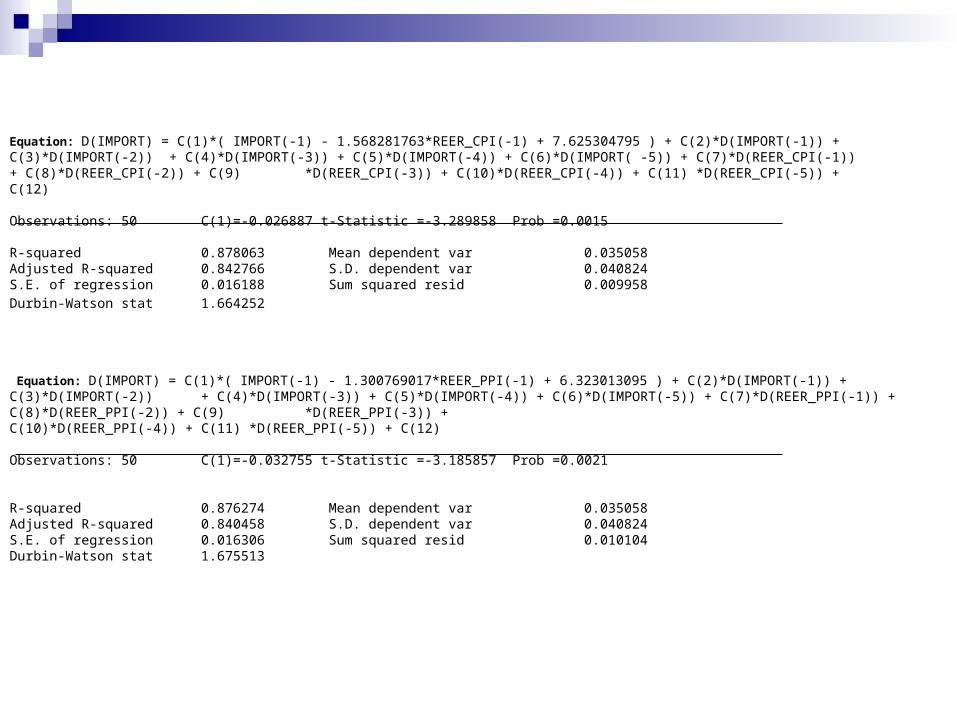
Results of regression for the two types of REER

back

Newey-West HAC Standard Errors & Covariance (lag truncation=3)

Export= REER_CPI*2.714627-13.4857 R-squared 0.735833 D-W=0.25 [7.37] [-7.15]Export= REER_PPI*3.058773-15.33536 R-squared 0.677775 D-W=0.24 [6.98] [-6.83]

Import =REER_CPI*2.726184-13.44575 R-squared 0.863549 D-W=0.47 [10.88] [-10.57]Import =REER_PPI*3.121839-15.55607 R-squared 0.821542 D-W=0.45 [10.22] [-9.97]

1.072.714627 =1.2016 ≈20.16% and 1.043.058773 =1.1274 ≈12,74 % respectively the volume of Export

1.072.726184 =1.2025 ≈ 20.25 % and 1.043.121839 =1.13025≈13% the volume of Import

0.932.714627 =0.8211 ≈ 17% and 0.963.058773 =0.8826 ≈11% respectively the volume of Export

0.932.726184 = 0.82050≈ 18% and 0.963.121839 = 0.8803≈ 12% the volume of Import

Error Correction: D(EXPORT) D(REER_CPI)

CointEq1 -0.026831 0.037366 -0.00796 -0.03473 [-3.37139] [ 1.07602] D(EXPORT(-1)) 1.739403 0.396493 -0.14054 -0.61324 [ 12.3764] [ 0.64655] D(EXPORT(-2)) -0.995528 -1.626568 -0.24651 -1.07564 [-4.03844] [-1.51219] D(EXPORT(-3)) 0.011508 1.097897 -0.194 0.396493 [ 0.05932] -0.8465 D(EXPORT(-4)) 0.135763 0.663789 -0.17803 -0.77681 [ 0.76259] [ 0.85451] D(EXPORT(-5)) 0.034147 -0.751968 -0.10317 -0.45017 [ 0.33098] [-1.67041] D(REER_CPI(-1)) -0.028347 -0.031705 -0.04203 -0.18341 [-0.67439] [-0.17286] D(REER_CPI(-2)) -0.015701 -0.032804 -0.03904 -0.17034 [-0.40218] [-0.19258] D(REER_CPI(-3)) -0.003189 -0.071179 -0.03615 -0.15774 [-0.08820] [-0.45123] D(REER_CPI(-4)) 0.008532 0.661299 -0.03446 -0.15035 [ 0.24760] [ 4.39840] D(REER_CPI(-5)) -0.022911 -0.034658 -0.03963 -0.17293 [-0.57809] [-0.20041] C 0.003103 0.010857 -0.00252 -0.01097 [ 1.23355] [ 0.98929] R-squared 0.977714 0.599403 Adj. R-squared 0.971262 0.483441

Error Correction: D(EXPORT) D(REER_PPI)

CointEq1 -0.028198 0.018593 -0.00748 -0.03499 [-3.76757] [ 0.53144] D(E XPORT(-1)) 1.686887 0.188421 -0.14096 -0.65892 [ 11.9670] [ 0.28595] D(E XPORT(-2)) -0.929841 -1.221119 -0.24379 -1.1396 [-3.81409] [-1.07153] D(E XPORT(-3)) -0.015874 0.872541 -0.18797 -0.87866 [-0.08445] [ 0.99304] D(E XPORT(-4)) 0.103608 0.435582 -0.17251 -0.80639 [ 0.60060] [ 0.54016] D(E XPORT(-5)) 0.067053 -0.576815 -0.10082 -0.47129 [ 0.66506] [-1.22390] D(REER_PPI(-1)) -0.050379 -0.074302 -0.04334 -0.20259 [-1.16241] [-0.36676] D(REER_PPI(-2)) -0.035705 -0.143763 -0.04212 -0.1969 [-0.84768] [-0.73015] D(REER_PPI(-3)) -0.018617 -0.188018 -0.03819 -0.17852 [-0.48748] [-1.05320] D(REER_PPI(-4)) -0.00479 0.522877 -0.03568 -0.1668 [-0.13423] [ 3.13484] D(REER_PPI(-5)) -0.027285 -0.130857 -0.03782 -0.17679 [-0.72145] [-0.74019] C 0.004179 0.018002 -0.0025 -0.01171 [ 1.66879] [ 1.53771] R-squared 0.979022 0.545854 Adj. R-squared 0.972949 0.414391

Export and REER

Error Correction: D(IMPORT) D(REER_CPI)

CointEq1 -0.032755 -0.027104 -0.01028 -0.02632 [-3.18586] [-1.02964] D(IMPORT(-1)) 0.745684 -0.30989 -0.14289 -0.36585 [ 5.21865] [-0.84704] D(IMPORT(-2)) 0.074828 0.009553 -0.15227 -0.38988 [ 0.49141] [ 0.02450] D(IMPORT(-3)) 0.09975 0.415445 -0.12756 -0.3266 [ 0.78200] [ 1.27203] D(IMPORT(-4)) -0.559474 0.080728 -0.13069 -0.33461 [-4.28104] [ 0.24126] D(IMPORT(-5)) 0.182278 -0.344243 -0.11005 -0.28177 [ 1.65636] [-1.22173] D(REER_CPI(-1)) -0.048302 -0.068509 -0.06324 -0.16192 [-0.76377] [-0.42310] D(REER_CPI(-2)) -0.022826 -0.207774 -0.05791 -0.14828 [-0.39415] [-1.40123] D(REER_CPI(-3)) -0.025285 -0.2286 -0.05557 -0.14229 [-0.45499] [-1.60661] D(REER_CPI(-4)) 0.0006 0.508509 -0.05446 -0.13944 [ 0.01101] [ 3.64678] D(REER_CPI(-5)) 0.009193 -0.252885 -0.06222 -0.15932 [ 0.14774] [-1.58731] C 0.017404 0.018448 -0.00452 -0.01159 [ 3.84629] [ 1.59233] R-squared 0.878063 0.546659 Adj. R-squared 0.842766 0.415429

Error Correction: D(IMPORT) D(REER_PPI)

CointEq1 -0.026887 -0.032249 -0.00817 -0.02089 [-3.28986] [-1.54376] D(IMPORT(-1)) 0.755633 -0.492515 -0.14285 -0.36514 [ 5.28964] [-1.34885] D(IMPORT(-2)) 0.06916 0.175768 -0.15294 -0.39092 [ 0.45221] [ 0.44963] D(IMPORT(-3)) 0.088999 0.336445 -0.12843 -0.32827 [ 0.69299] [ 1.02491] D(IMPORT(-4)) -0.562758 0.140002 -0.13091 -0.3346 [-4.29894] [ 0.41841] D(IMPORT(-5)) 0.196872 -0.354086 -0.10993 -0.28098 [ 1.79094] [-1.26018] D(REER_PPI(-1)) -0.048784 -0.088648 -0.06184 -0.15807 [-0.78887] [-0.56082] D(REER_PPI(-2)) -0.035428 -0.252976 -0.05779 -0.14771 [-0.61305] [-1.71261] D(REER_PPI(-3)) -0.028545 -0.287974 -0.05585 -0.14276 [-0.51108] [-2.01717] D(REER_PPI(-4)) -0.023677 0.429441 -0.05541 -0.14163 [-0.42732] [ 3.03218] D(REER_PPI(-5)) 0.004645 -0.284672 -0.06083 -0.15548 [ 0.07636] [-1.83089] C 0.017544 0.020442 -0.00448 -0.01144 [ 3.91921] [ 1.78657] R-squared 0.876274 0.518917 Adj. R-squared 0.840458 0.379657

Import and REER

Error correction equations:

Equation: D(EXPORT) = C(1)*( EXPORT(-1) - 3.505269075*REER_CPI(-1) + 17.52164625 ) + C(2)*D(EXPORT(-1)) + C(3)*D(EXPORT(-2))+ C(4)*D(EXPORT(-3)) + C(5)*D(EXPORT(-4)) + C(6)*D(EXPORT(-5)) + C(7)*D(REER_CPI(-1)) + C(8)*D(REER_CPI(-2)) + C(9)*D(REER_CPI(-3)) + C(10)*D(REER_CPI(-4)) + C(11) *D(REER_CPI(-5)) + C(12)

Observations:50 C(1)=-0.026831 t-Statistic =-3.37139 Prob =0.0012

R-squared 0.977714 Mean dependent var 0.032526

Adjusted R-squared 0.971262 S.D. dependent var 0.052673

S.E. of regression 0.008929 Sum squared resid 0.003030

Durbin-Watson stat 2.013430

Estimation Method: Least SquaresSample: 1991:3 2003:4Included observations: 50 Total system (balanced) observations 100

Equation: D(EXPORT) = C(1)*( EXPORT(-1) - 4.165968926*REER_PPI( -1) + 21.01019822 ) + C(2)*D(EXPORT(-1)) + C(3)*D(EXPORT(-2)) + C(4)*D(EXPORT(-3)) + C(5)*D(EXPORT(-4)) + C(6)*D(EXPORT(-5)) + C(7)*D(REER_PPI(-1)) + C(8)*D(REER_PPI(-2)) + C(9) *D(REER_PPI(-3)) + C(10)*D(REER_PPI(-4)) + C(11) *D(REER_PPI(-5)) + C(12)

Observations: 50 C(1)=-0.028198 t-Statistic =-3.767567 Prob =0.0003

R-squared 0.979022 Mean dependent var 0.032526

Adjusted R-squared 0.972949 S.D. dependent var 0.052673

S.E. of regression 0.008663 Sum squared resid 0.002852


Equation: D(IMPORT) = C(1)*( IMPORT(-1) - 1.568281763*REER_CPI(-1) + 7.625304795 ) + C(2)*D(IMPORT(-1)) + C(3)*D(IMPORT(-2)) + C(4)*D(IMPORT(-3)) + C(5)*D(IMPORT(-4)) + C(6)*D(IMPORT( -5)) + C(7)*D(REER_CPI(-1)) + C(8)*D(REER_CPI(-2)) + C(9) *D(REER_CPI(-3)) + C(10)*D(REER_CPI(-4)) + C(11) *D(REER_CPI(-5)) + C(12)


R-squared 0.878063 Mean dependent var 0.035058Adjusted R-squared 0.842766 S.D. dependent var 0.040824S.E. of regression 0.016188 Sum squared resid 0.009958


Equation: D(IMPORT) = C(1)*( IMPORT(-1) - 1.300769017*REER_PPI(-1) + 6.323013095 ) + C(2)*D(IMPORT(-1)) + C(3)*D(IMPORT(-2)) + C(4)*D(IMPORT(-3)) + C(5)*D(IMPORT(-4)) + C(6)*D(IMPORT(-5)) + C(7)*D(REER_PPI(-1)) + C(8)*D(REER_PPI(-2)) + C(9) *D(REER_PPI(-3)) + C(10)*D(REER_PPI(-4)) + C(11) *D(REER_PPI(-5)) + C(12)


R-squared 0.876274 Mean dependent var 0.035058Adjusted R-squared 0.840458 S.D. dependent var 0.040824S.E. of regression 0.016306 Sum squared resid 0.010104Durbin-Watson stat 1.675513

Results of regressions:

EXPORT =REER_CPI *0.565837+GDP_EU*0.390866 -0.971709 R-squared 0.691239 , D-W=0.54 [3.57] [2.71] [- 1.26]

EXPORT =REER_PPI *0.441380+GDP_EU*0.507131 -0.887198 R-squared 0.608194 , D-W=0.38 [3.16] [3.26] [-1.11]

IMPORT=REER_CPI*-0.095769+EXPORT*0.802969+AGR_DEMAND*0.048147+ 1.078879 R-squared 0.961766 , D-W=0.28 [-1.59] [16.92] [1.33] [3.66]

IMPORT=REER_PPI*-0.007240+EXPORT*0.793771+AGR_DEMAND*0.023037+ 1.078879 R-squared 0.969995 , D-W=0.25 [-0.137] [15.98] [0.48] [2.42]

REER influence on Trade Balance

VAR Lag Order Selection Criteria Endogenous variables: TB, REER_CPI Exogenous variables: C Sample: 1990:1 2003:4 Included observations: 44


0 17.70244 NA 0.001679 -0.713747 -0.632648 -0.683672 1 88.67878 132.2741 8.00E-05 -3.758126 -3.514828 -3.6679 2 91.89628 5.703744 8.30E-05 -3.722558 -3.317061 -3.57218 3 94.40193 4.214051 8.92E-05 -3.654633 -3.086937 -3.444104 4 104.8354 16.59863 6.70E-05 -3.947062 -3.217166 -3.676381 5 131.8029 40.45131 2.38E-05 -4.991041 -4.098946 -4.660209 6 141.2231 13.27391 1.89E-05 -5.237413 -4.183119 -4.84643 7 151.3592 13.36123* 1.46E-05 -5.516327 -4.299834* -5.065193* 8 154.7967 4.218743 1.54E-05 -5.490759 -4.112067 -4.979473 9 157.2011 2.73231 1.72E-05 -5.418233 -3.877342 -4.846796

10 161.4021 4.391939 1.78E-05 -5.427369 -3.724278 -4.795781 11 167.3322 5.660496 1.74E-05 -5.515098 -3.649809 -4.823359 12 177.3208 8.626542 1.4E-05* -5.787308* -3.75982 -5.035418


VAR Lag Order Selection Criteria Endogenous variables: TB, REER_PPI Exogenous variables: C Sample: 1990:1 2003:4 Included observations: 44


0 25.93637 NA 0.001155 -1.088017 -1.006918 -1.057941 1 90.80959 120.9001 7.26E-05 -3.854981 -3.611683 -3.764755 2 93.2591 4.342315 7.80E-05 -3.784505 -3.379007 -3.634127 3 95.20509 3.272803 8.60E-05 -3.691141 -3.123444 -3.480611 4 104.053 14.07614 6.94E-05 -3.911498 -3.181602 -3.640817 5 127.3334 34.92065 2.92E-05 -4.787881 -3.895786 -4.457049 6 137.2678 13.9985 2.26E-05 -5.057627 -4.003333 -4.666644 7 147.7789 13.85551 1.72E-05 -5.353585 -4.137092* -4.902451* 8 151.4471 4.501931 1.79E-05 -5.338505 -3.959813 -4.82722 9 154.1415 3.061851 1.97E-05 -5.279161 -3.73827 -4.707725

10 157.5464 3.55959 2.12E-05 -5.252108 -3.549018 -4.62052 11 169.0374 10.96870* 1.61E-05* -5.592609* -3.727319 -4.900869 12 172.6375 3.10918 1.77E-05 -5.574431 -3.546943 -4.822541


Romania has negative Trade Balance (TB) with EU countriesVAR lag length criteria : 7 lags for both REER_CPI and REER_PPI

relationship with TB

REER influence on Trade Balance

cointegration equation for 5% level of significance for the two cases TB and REER_CPI and TB and REER_PPI

Lags interval (in first differences): 1 to 7

Unrestricted Cointegration Rank Test

Hypothesized Max-Eigen 5 Percent 1 Percent No. of CE(s) Eigenvalue Statistic Critical Value Critical Value

None ** 0.316328 19.01385 18.96 23.65 At most 1 0.053405 2.744201 12.25 16.26

*(**) denotes rejection of the hypothesis at the 5%(1%) level Max-eigenvalue test indicates 1 cointegrating equation(s) at the 5% level


None ** 0.241673 14.01937 12.53 16.31 At most 1 0.015312 0.740640 3.84 6.51

*(**) denotes rejection of the hypothesis at the 5%(1%) level Trace test indicates 1 cointegrating equation(s) at 5% level

Pairwise Granger Causality Tests:

Sample: 1990:1 2003:4

Lags: 1 Null Hypothesis: Obs F-Statistic ProbabilityREER_CPI does not Granger Cause TB 55 9.52595 0.00324TB does not Granger Cause REER_CPI 0.02620 0.87203

Lags: 2Null Hypothesis: Obs F-Statistic ProbabilityREER_CPI does not Granger Cause TB 54 2.32283 0.10869TB does not Granger Cause REER_CPI 0.02812 0.97229

Lags: 1Null Hypothesis: Obs F-Statistic ProbabilityREER_PPI does not Granger Cause TB 55 9.19004 0.00379TB does not Granger Cause REER_PPI 0.01979 0.88866

Lags: 2Null Hypothesis: Obs F-Statistic ProbabilityREER_PPI does not Granger Cause TB 54 2.31398 0.10958TB does not Granger Cause REER_PPI 0.02818 0.97223

Results of regressions for the two types of REER

TB=REER_CPI*1.65779 -8.692956 R-squared 0.441621 , D-W=0.79

[3.6841] [-3.8573]

TB=REER_PPI*1.92424 -9.293298 R-squared 0.431312 , D-W=0.78

[3.6981] [-3.8518]

1.071.65 =1.118 ≈11.8 % and 1.041.92 =1.078 ≈7.8 % 0.931.65 =0.887 ≈ 12 % and 0.961.92 =0.92 ≈8 %

TB does not have the expected sign and consequently it initially worsens at REER depreciations and then it improves (starting with lag 4 it has the expected negative sign)

TB and REER_CPI (7 lags):

D(TB) = 0.1370008082*( TB(-1) + 0.01767896916*REER_CPI_LOG(-1) ) + 0.7865814588*D(TB(-1)) - 0.3968784339*D(TB(-2)) + 0.03360259529*D(TB(-3)) - 0.2447805494*D(TB(-4)) -0.04381380141*D(TB(-5)) - 0.04652583436*D(TB(-6)) - 0.1803369447*D(TB(-7)) +3.425845879*D(REER_CPI (-1)) – 0.8003956003*D(REER_CPI (-2)) +1.207371803*D(REER_CPI (-3)) +1.756795848*D(REER_CPI (-4)) - 3.157573105*D(REER_CPI (-5)) + 2.403071583*D(REER_CPI (-6)) - 0.01985208971*D(REER_CPI (-7))

D(REER_CPI) = - 0.06954231854*( TB(-1) + 0.01767896916*REER_CPI(-1) ) –0.07424238375*D(TB(-1)) + 0.1036032247*D(TB(-2)) +0.005701677302*D(TB(-3)) +0.03426812401*D(TB(-4)) + 0.01956357912*D(TB(-5)) + 0.05240118994*D(TB(-6)) +0.04620054128*D(TB(-7)) - 0.5301569997*D(REER_CPI(-1)) + 0.02040601877*D(REER_CPI(-2)) –0.4077126554*D(REER_CPI(-3)) + 0.3907634519*D(REER_CPI(-4)) +0.1055090966*D(REER_CPI(-5)) - 0.5415890667*D(REER_CPI(-6)) +0.03241797129*D(REER_CPI(-7))

TB and REER_PPI (7 lags):

D(TB) = 0.1453655075*( TB(-1) + 0.2806808741*REER_PPI(-1) - 1.039744678 ) + 0.7616830328*D(TB(-1)) - 0.5830842106*D(TB(-2)) + 0.1383830284*D(TB(-3)) - 0.2598415963*D(TB(-4)) - 0.006246235075*D(TB(-5)) - 0.08143625724*D(TB(-6)) - 0.1648990411*D(TB(-7)) + 3.078886096*D(REER_PPI(-1)) - 1.223630924*D(REER_PPI(-2)) + 1.706903517*D(REER_PPI(-3)) + 1.682785129*D(REER_PPI(-4)) - 2.927038695*D(REER_PPI(-5)) + 2.73469155*D(REER_PPI(-6)) - 0.8225060185*D(REER_PPI(-7)) - 0.00491755967

D(REER_PPI) = - 0.07763000086*( TB(-1) + 0.2806808741*REER_PPI(-1) - 1.039744678 ) - 0.04419584655*D(TB(-1)) + 0.1514702121*D(TB(-2)) - 0.01653847494*D(TB(-3)) + 0.03061622078*D(TB(-4)) + 0.01204721762*D(TB(-5)) + 0.05570758654*D(TB(-6)) + 0.04820989632*D(TB(-7)) - 0.4477123584*D(REER_PPI(-1)) + 0.03722262183*D(REER_PPI(-2)) - 0.5756806286*D(REER_PPI(-3)) + 0.2824755348*D(REER_PPI(-4)) - 0.0615261533*D(REER_PPI(-5)) - 0.6419286947*D(REER_PPI(-6)) + 0.161200314*D(REER_PPI(-7)) + 0.01206296165

Error Correction Model

Dependent Variable: D(TB)Method: Least Squares

Sample(adjusted): 1992:1 2003:4

Included observations: 48 after adjusting endpoints

D(TB) = C(1)*( TB(-1) + 0.01069773101*REER_CPI(-1) + 0.2191682532 ) + C(2)*D(TB(-1)) + C(3)*D(TB(-2)) + C(4)*D(TB(-3)) + C(5)*D(TB( -4)) + C(6)*D(TB(-5)) + C(7)*D(TB(-6)) + C(8)*D(TB(-7)) + C(9) *D(REER_CPI(-1)) + C(10)*D(REER_CPI(-2)) + C(11)*D(REER_CPI(-3)) + C(12)*D(REER_CPI(-4)) + C(13) *D(REER_CPI(-5)) + C(14)*D(REER_CPI(-6)) + C(15) *D(REER_CPI(-7)) + C(16)

Coefficient Std. Error t-Statistic Prob.

C(1) 0.154977 0.087303 1.775161 0.0854C(2) 0.772608 0.225150 3.431524 0.0017C(3) -0.430887 0.253643 -1.698796 0.0991C(4) 0.042718 0.140261 0.304563 0.7627C(5) -0.252806 0.076088 -3.322545 0.0022C(6) -0.052952 0.085477 -0.619482 0.5400C(7) -0.063642 0.080023 -0.795298 0.4323C(8) -0.191026 0.071940 -2.655359 0.0122C(9) 3.421184 0.646882 5.288729 0.0000C(10) -0.841963 0.769861 -1.093657 0.2823C(11) 1.268492 0.664479 1.909003 0.0653C(12) 1.716229 0.449494 3.818133 0.0006C(13) -3.198078 0.704544 -4.539218 0.0001C(14) 2.399025 0.873477 2.746522 0.0098C(15) -0.156624 0.839850 -0.186491 0.8532C(16) -0.016135 0.026257 -0.614526 0.5432

R-squared 0.705076 Mean dependent var 0.022440Adjusted R-squared 0.566830 S.D. dependent var 0.169311S.E. of regression 0.111433 Akaike info criterion -1.289581Sum squared resid 0.397356 Schwarz criterion -0.665848Log likelihood 46.94995 Durbin-Watson stat 2.087974

White Heteroskedasticity Test: F-statistic 1.788021 Probability 0.116205Jarque-Bera normality Test: Statistic 2.391790 Probability 0.302433

Dependent Variable: D(TB)Method: Least Squares

Sample(adjusted): 1992:1 2003:4Included observations: 48 after adjusting endpoints

D(TB) = C(1)*( TB(-1) + 0.3370609842*REER_PPI(-1) - 1.444550447 ) + C(2)*D(TB(-1)) + C(3)*D(TB(-2)) + C(4)*D(TB(-3)) + C(5)*D(TB(-4)+ C(6)*D(TB(-5)) + C(7)*D(TB(-6)) + C(8)*D(TB(-7)) + C(9) *D(REER_PPI(-1)) + C(10)*D(REER_PPI(-2)) + C(11 ) *D(REER_PPI(-3)) + C(12)*D(REER_PPI(-4)) + C(13) *D(REER_PPI(-5)) + C(14)*D(REER_PPI(-6)) + C(15)

*D(REER_PPI(-7)) + C(16) Coefficient Std. Error t-Statistic Prob.

C(1) 0.146502 0.074730 1.960429 0.0587C(2) 0.645211 0.208309 3.097381 0.0040C(3) -0.472682 0.226722 -2.084853 0.0451C(4) 0.098739 0.133076 0.741979 0.4635C(5) -0.265859 0.073777 -3.603558 0.0011C(6) -0.022232 0.084235 -0.263930 0.7935C(7) -0.076169 0.077014 -0.989016 0.3301C(8) -0.156350 0.068061 -2.297198 0.0283C(9) 2.884267 0.560499 5.145893 0.0000C(10) -0.906927 0.690607 -1.313232 0.1984C(11) 1.541538 0.586483 2.628445 0.0131C(12) 1.775626 0.459297 3.865960 0.0005C(13) -2.656261 0.619329 -4.288936 0.0002C(14) 2.369020 0.781475 3.031472 0.0048C(15) -0.509762 0.766876 -0.664725 0.5110C(16) -0.006860 0.024101 -0.284647 0.7777

R-squared 0.704920 Mean dependent var 0.022440Adjusted R-squared 0.566601 S.D. dependent var 0.169311S.E. of regression 0.111463 Akaike info criterion -1.289052Sum squared resid 0.397566 Schwarz criterion -0.665318Log likelihood 46.93725 Durbin-Watson stat 2.215315

White Heteroskedasticity Test : F-statistic 1.687595 Probability 0.141207Jarque-Bera normality Test: Statistic 6.482801 Probability 0.039109

Conclusions Results show that is possible to start building a quantitative background for

discussion about REER in Romania during the accession process

REER is a useful summary indicator of essential economic information

REER can be a good indicator for monetary and exchange rate policies in order to forecast trade balance in a country (R-squared ≈ 70%)

Exports and Imports have the expected reaction to REER movements

Trade Balance initially worsens after a REER depreciation and then it improves

It is questionable whether permanent depreciation is desirable to improve trade balance

Romanian “ Trade Openness” to GDP ratio

68.0%70.0%72.0%74.0%76.0%78.0%80.0%82.0%84.0%86.0%

2001 2002 2003

period

Weight in GDP

Romanian Trade volumes

02000400060008000

100001200014000

1990

1992

1994

1996

1998

2000

2002

period

mil

US

D

export with EU

export with Europe

Total export

back

Source: Romanian External Trade Department

Date post:	21-Dec-2015
Category:	Documents
View:	217 times
Download:	4 times

Dissertation Paper Real effective exchange rates and their influence on Romania’s trade with...

Documents