Dissipative Dynamics of atomic Bose-Einstein condensates at zero temperature by Zhigang Wu A thesis submitted to the Department of Physics, Engineering Physics and Astronomy in conformity with the requirements for the degree of Doctor of Philosophy Queen’s University Kingston, Ontario, Canada April 2013 Copyright c Zhigang Wu, 2013
Transcript
Dissipative Dynamics of atomic Bose-Einstein
condensates at zero temperature
by
Zhigang Wu
A thesis submitted to the
Department of Physics, Engineering Physics and Astronomy
Chapter 3: Density response functions 543.1 Definition and general properties of the density response function . . 553.2 Density response function within Bogoliubov theory . . . . . . . . . . 603.3 Examples of density response functions . . . . . . . . . . . . . . . . . 63
where Eq. (2.39) and Eq. (2.41) are used. Inserting Eq. (2.87) and Eq. (2.88) into
the above equation, we find
nH(r, t) = n0(r) +∑
i
[Φ0(r)ψ−i (r)e−iǫit/hb†0βi + h.c.], (2.99)
where ψ−i (r) ≡ ui(r) − vi(r).
Now we suppose that the condensate is in a normalized initial state of the form
|Ψ〉 = c0|Ψ0〉 + cj |Ψj〉, (2.100)
where |Ψj〉 = b0β†j |Ψ0〉 is an excited state containing one Bogoliubov quasi-particle.
Clearly this initial state is a non-equilibrium state in which the density deviates
from its value in the ground state. Using Eqs. (2.99) and (2.100) we find that the
subsequent temporal evolution of the density is given by
〈Ψ|nH(r, t)|Ψ〉 = n0(r) + δnj(r, t), (2.101)
2.4. COLLECTIVE EXCITATIONS: HYDRODYNAMIC THEORY 39
where
δnj(r, t) = c∗0cjδnj(r)e−iǫjt/h + c.c. (2.102)
with
δnj(r) = Φ0(r)ψ−j (r). (2.103)
This shows that the density fluctuation of the condensate in this particular dynamic
state oscillates with a frequency ωj = ǫj/h and with an amplitude that is proportional
to δnj(r). Using Eq. (2.99) and the fact that n(r) = nH(r, t = 0), it is easy to show
that
δnj(r) = 〈Ψ0|n(r)|Ψj〉. (2.104)
The foregoing analysis implies that the energies of the excitations and the Bo-
goliubov amplitudes can be measured experimentally by exciting the condensate in
definite ways and recording its density oscillations. Indeed many low-lying excitations
have been measured in this way and they are found to be in good agreement with
theoretical predictions based on Bogoliubov theory [11].
2.4 Collective excitations: Hydrodynamic theory
We have seen in the previous section that there is an intimate connection between
the Bogoliubov excitations and the density fluctuations in non-equilibrium states of
the system. Indeed, we shall see that the energies of the Bogliubov quasi-particles
and the associated Bogoliubov amplitudes can be found alternatively by means of
the hydrodynamic equations, which describe the temporal evolution of the density
fluctuation δn(r, t) and the velocity field v(r, t) of the condensate. Quite generally,
2.4. COLLECTIVE EXCITATIONS: HYDRODYNAMIC THEORY 40
the density fluctuation δn(r, t) and the velocity field v(r, t) can be expressed in terms
of the expectation values of the Heisenberg density operator nH(r, t) and the current
density operator jH(r, t), namely2
δn(r, t) = 〈nH(r, t)〉 − n0(r); (2.105)
v(r, t) =1
n0(r)〈jH(r, t)〉, (2.106)
where the average is taken with respect to the initial many-body state of the system
|Ψ〉. As shown earlier, within Bogoliubov theory nH(r, t) is given by Eq. (2.98). To
find the current density operator within the same approximation, we write j(r) in the
second-quantization form
j(r) =h
2mi
[
ψ†(r)∇ψ(r) −∇ψ†(r)ψ(r)]
. (2.107)
To first order in field fluctuation operators, we find
j(r) =h
2mi
[
Φ0b†0∇δψ + ∇Φ0b0δψ
† −∇Φ0b†0δψ − Φ0b0∇δψ†
]
=h
2min0(r)∇
(
1
Φ0(r)
[
b†0δψ(r) − b0δψ†(r)]
)
, (2.108)
where Φ0(r) is again taken to be real. The Heisenberg current density operator is
then given by
jH(r, t) =h
2min0(r)∇
(
1
Φ0(r)[b†0δψK(r, t) − b0δψ
†K(r, t)]
)
. (2.109)
2Strictly speaking, the velocity field v(r, t) is defined by the relation 〈jH(r, t)〉 = 〈nH(r, t)〉v(r, t).However, the definition in Eq. (2.106) amounts to a linearization of this relation and is consistentwith the Bogoliubov theory.
2.4. COLLECTIVE EXCITATIONS: HYDRODYNAMIC THEORY 41
Eq. (2.98) and Eq. (2.109) imply that within Bogoliubov theory, the time-evolution of
δn(r, t) and v(r, t) are essentially determined by the time-evolution of the field fluc-
tuation operators. In other words, the hydrodynamic equations satisfied by δn(r, t)
and v(r, t) can be derived by means of the Heisenberg equations of motion for these
fluctuation operators given in Eq. (2.36) and Eq. (2.38).
Using Eq. (2.98) and Eq. (2.105) we find
∂
∂tδn(r, t) = Φ0(r)
⟨
b†0∂
∂tδψK(r, t) + b0
∂
∂tδψ†
K(r, t)
⟩
. (2.110)
Substituting Eqs. (2.36) and (2.38) into the above equation and using the GP equa-
To obtain the dipole potential, we substitute the above expression into Eq. (2.131) and
perform the average over a period of time π/(ω1+ω2). Since (ω1−ω2)/2 ≪ (ω1+ω2)/2,
the effect of time-average on
cos2
(
ω1 − ω2
2t− k1 − k2
2· r)
can be neglected. With an appropriate energy reference point, we obtain the following
2.5. OPTICAL DIPOLE POTENTIAL 49
dipole potential
VBragg(r, t) = VB cos (ωBt− kB · r) , (2.135)
where ωB = ω1−ω2 and kB = k1−k2. This potential moves in the direction of kB with
a velocity vB = ωB/kB which can be controlled by adjusting the angle between the
directions of propagation of the two laser beams. A slow modulation of the amplitude
VB can be used to generate a Bragg pulse.
2.5.3 Disorder potential for atomic clouds: optical speckle pattern
Unlike solid state systems, cold atomic systems are intrinsically clean. Thus in or-
der to study the interplay between disorder and particle interactions in cold atom
experiments, some form of disorder potential has to be introduced into the system.
Because of the fragile nature of these atomic systems, the disorder potential needs to
be well controlled and calibrated. A random light intensity pattern formed after a
laser passes through a diffusive medium, provides one ideal implementation of such
a disorder potential. A typical example of a diffusive medium is a ground glass plate
with an optically rough surface. When a coherent light beam is passed through such
a plate, each point on the surface can be viewed as a secondary source of radiation
(Huygens Principle). The surface roughness imparts a random phase to each sec-
ondary source. Thus, when the radiation from all the sources is superposed on an
observation plane, the interference of all the waves produces a randomly distributed
pattern of light. This pattern is referred to as optical speckle.
Shown in Fig. 2.1 is a typical experimental setup for producing a disorder potential
on a Bose condensate. A laser beam is shone through a diffusive plate and produces
an optical speckle pattern, which is imaged onto a cold atomic system. The speckle
2.5. OPTICAL DIPOLE POTENTIAL 50
gives rise to a static disorder dipole potential Vdis(r). The effect of this disorder
potential on the atomic cloud is then observed by means of an imaging beam.
mm
150
(b)
(a)
CCD
imaging beam
speckle beam
diffusive plate
dichroic mirror
BEC cell
Figure 2.1: (a) Experimental setup for the speckle potential and the imaging systemfor a BEC. (b) The intensity distribution of the speckle potential in a 2Dplane (left) and its Fourier transform (right). Figures taken from [16].
Two important statistical properties of a speckle pattern are the standard devia-
tion of the light intensity in space and the two-point light intensity auto-correlation
function. As explained in [46], the statistical distribution of the light intensity I(r)
in space follows an exponential distribution
P (I) =1
Ie−I/I , (2.136)
where I is the mean value of the intensity. From this distribution the standard
2.5. OPTICAL DIPOLE POTENTIAL 51
deviation of the light intensity σI ≡√
I2 − I2 is found to be the same as I. The
intensity auto-correlation function is defined as
γI(r) = I(r′)I(r′ + r), (2.137)
where the overbar denotes a spatial average with respect to the variable r′.3 Since
σI = I, Eq. (2.137) can be rewritten as
γI(r) = I2[1 + C(r)], (2.138)
where the function C(r) has the property that C(r = 0) = 1.
Since the dipole potential is proportional to the light intensity, the statistical
properties of the disorder potential follow from those of the speckle light pattern.
The standard deviation of the disorder potential
VD ≡√
V 2dis(r) − Vdis(r)
2= Vdis(r) (2.139)
is often referred to as the strength of the disorder potential. From Eq. (2.138) we see
that the auto-correlation function of the disorder potential is given by
γV (r) = V 2D[1 + C(r)], (2.140)
The correlation function C(r) typically decays as a function of r and its widths
in the x, y and z directions characterize the typical size of a speckle grain. These
3The spatial average can equivalently be viewed as an ensemble average. For an ensemble repre-senting a translationally invariant system, the resulting average is independent of r′.
2.5. OPTICAL DIPOLE POTENTIAL 52
widths can be adjusted experimentally to produce an effectively one-dimensional dis-
order potential. For instance, let us consider a condensate that is elongated in the z
direction. If the size of the speckle grains in the transverse direction is much larger
than the transverse TF radius R⊥ of the cloud, the disorder potential produced by the
speckle pattern can be viewed as effectively one-dimensional (along the z direction).
In this situation C(r) = C(z). To a good approximation, C(z) is given by [46]
C(z) = e−(z/σ)2 , (2.141)
where σ is sometimes referred to as the disorder correlation length.
As we shall see, it is useful to express the statistical properties of the one-
dimensional disorder potential in terms of the Fourier components of the potential
Vdis(r),
Vdis(q) =
∫
dre−iq·rVdis(r). (2.142)
The ensemble average of this quantity is
Vdis(q) =
∫
dre−iq·rVdis(r) = (2π)3δ(q)VD. (2.143)
Similarly, we have
V ∗dis(q)Vdis(q′) =
∫
dr
∫
dr′eiq·re−iq′·r′Vdis(r)Vdis(r′)
=
∫
drei(q−q′)·r∫
dse−iq′·sγV (s)
= (2π)3δ(q − q′)V 2D[(2π)3δ(q) + C(q)], (2.144)
2.5. OPTICAL DIPOLE POTENTIAL 53
where C(q) is the Fourier transform of C(r). For the one-dimensional correlation
function we have
C(q) =
∫
dre−iq·rC(r)
= (2π)2δ(qx)δ(qy)σ√πe−
14σ2q2
z . (2.145)
These results will be used in Chapter 5.
Figure 2.2: (a) The profile of a one-dimensional disorder potential produced by aspeckle pattern. The disorder strength is indicated by half of the distancebetween the two horizontal lines. (b) The auto-correlation function of thedisorder potential in (a). Figures taken from [23].
Finally, we point out that both the disorder strength and the auto-correlation
function can be measured accurately in experiments. Fig. 2.2 (a) shows an example
of the spatial variation of a one-dimensional disorder potential. The corresponding
auto-correlation function is shown in Fig. 2.2 (b). The correlation length is about
10µm which is comparable to the average distance between the peaks in Fig. 2.2 (a).
54
Chapter 3
Density response functions
In this chapter we present detailed calculations of zero-temperature density response
functions of Bose-Einstein condensates within the Bogoliubov theory. We will con-
sider condensates having a uniform density as well as those in trapped geometries.
These density response functions will be used extensively in later chapters when
we investigate the dissipative dynamics of condensates using linear response theory.
Within the Bogoliubov approximation, the zero-temperature density response func-
tion of a Bose condensate can be expressed in terms of the Bogoliubov amplitudes
and hence its determination becomes a matter of solving the Bogoliubov-de Gennes
equations. It is relatively straightforward to carry out such calculations for both the
uniform condensate and the uniform cylindrical condensate. However, the numerical
calculations are much more difficult for an arbitrary trapped gas. Nevertheless, for
an elongated condensate we can invoke a local density approximation which makes
use of the response properties of a uniform cylindrical condensate. The formulation
of this approximation and its justification will be explained.
3.1. DEFINITION AND GENERAL PROPERTIES OF THEDENSITY RESPONSE FUNCTION 55
3.1 Definition and general properties of the density response function
The zero-temperature density response function for the atomic Bose-Einstein conden-
sate, described by the Hamiltonian H given in Eq. (2.24), is defined as
χ(r, r′, t− t′) =i
hθ(t− t′)〈Ψ0|[nH(r, t), nH(r′, t′)]|Ψ0〉, (3.1)
where |Ψ0〉 denotes the ground state of H and n(r, t) is the density operator in the
Heisenberg picture nH(r, t) = eiHt/hn(r)e−iHt/h. One can obtain a more explicit
expression by making use of the closure relation∑
m |Ψm〉〈Ψm| = 1, where |Ψm〉 is
an eigenstate of H with energy Em. The insertion of this relation in Eq. (3.1) leads
to the spectral representation
χ(r, r′, t− t′) =i
hθ(t− t′)
∑
m6=0
e−iωm0(t−t′)〈Ψ0|n(r)|Ψm〉〈Ψm|n(r′)|Ψ0〉 − c.c.
, (3.2)
where ωm0 ≡ (Em−E0)/h. The term withm = 0 can be excluded from the summation
since it gives a zero contribution. We emphasize that this is a general expression which
is applicable to any system in its ground state. It can be extended straightforwardly
to finite temperatures by making use of an appropriate statistical density matrix.
In calculations, Fourier transforms of the density response function are often more
useful. Since χ(r, r′, τ) for an inhomogeneous system depends on the two independent
variables r and r′, we define the double spatial Fourier transform
χ(q,q′, τ) ≡∫
dr
∫
dr′e−i(q·r−q′·r′)χ(r, r′, τ). (3.3)
3.1. DEFINITION AND GENERAL PROPERTIES OF THEDENSITY RESPONSE FUNCTION 56
Substituting Eq. (3.2) into the above definition one finds
χ(q,q′, τ) =i
hθ(τ)
∑
m6=0
e−iωm0τn0m(q)n∗0m(q′) − eiωm0τnm0(q)n∗
m0(q′)
,
=i
hθ(τ)
∑
m6=0
n0m(q)n∗0m(q′)
(
e−iωm0τ − eiωm0τ)
, (3.4)
where
nmn(q) = 〈Ψm|n(q)|Ψn〉 (3.5)
with
n(q) ≡∫
dre−iq·rn(r). (3.6)
In arriving at the second line of Eq. (3.4), we have used the fact that the sys-
tem possesses time-reversal symmetry. This symmetry implies that for each excited
state |Ψm〉 there exists a degenerate time-reversed state |Ψm〉 with the property that
〈Ψ0|n(r)|Ψm〉 = 〈Ψ0|n(r)|Ψm〉∗. As a result, nm0(q) = n0m(q) and, since a summa-
tion over m is equivalent to a summation over m, the second line of Eq. (3.4) follows.
Using the same reasoning, we can show that χ(q,q′, τ) has the property
χ(−q,−q′, τ) = χ(q,q′, τ). (3.7)
We now introduce the spectral function
S(q,q′, ω) ≡∑
m6=0
n0m(q)n∗0m(q′)δ(hω − hωm0). (3.8)
Since ωm0 > 0, we observe that the spectral function is zero for ω < 0. With this
3.1. DEFINITION AND GENERAL PROPERTIES OF THEDENSITY RESPONSE FUNCTION 57
definition, χ(q,q′; τ) can be written as
χ(q,q′, τ) = iθ(τ)
∫
dωS(q,q′, ω)(
e−iωτ − eiωτ)
. (3.9)
Using Eq. (3.9) and the following Fourier representation of the step function
θ(τ) = i limǫ→0
∫ ∞
−∞
dω
2π
e−iωτ
ω + iǫ, (3.10)
we obtain the Fourier transform
χ(q,q′, ω) ≡∫
dτeiωτχ(q,q′, τ)
=
∫
dω′S(q,q′, ω′)
(
1
ω + ω′ + iǫ− 1
ω − ω′ + iǫ
)
, (3.11)
where the positive, real infinitesimal ǫ ensures the causality of the response. The above
expression indicates that knowledge of the spectral function S(q,q′, ω) completely
determines the density response function.
Making use of the identity
1
x+ iǫ= P
1
x− iπδ(x), (3.12)
Eq. (3.11) can be written
χ(q,q′, ω) = χ′(q,q′, ω) + iχ′′(q,q′, ω), (3.13)
3.1. DEFINITION AND GENERAL PROPERTIES OF THEDENSITY RESPONSE FUNCTION 58
3.2. DENSITY RESPONSE FUNCTION WITHIN BOGOLIUBOVTHEORY 62
where we recall that the operator L is given in Eq. (2.37). Substituting Eq. (3.29)
into Eq. (3.28) we obtain
[n(q), HB] = b†0
∫
dre−iq·rΦ∗0Lδψ + gb0
∫
dre−iq·rΦ0|Φ0|2δψ†
− b0
∫
dre−iq·rΦ0Lδψ† − gb†0
∫
dre−iq·rΦ0|Φ0|2δψ. (3.30)
Since L is Hermitian we have
b†0
∫
dre−iq·rΦ∗0Lδψ = b†0
∫
dr[
L(
eiq·rΦ0
)]∗δψ
= b†0
∫
dre−iq·r[
h2q2
2mΦ∗
0 +ih2
mq · ∇Φ∗
0 + LΦ∗0
]
δψ
= b†0
∫
dre−iq·r[
h2q2
2mΦ∗
0 +ih2
mq · ∇Φ∗
0 + g|Φ0|2Φ∗0
]
δψ, (3.31)
where we used the GP equation (2.17) in the last line. Similarly we find
b0
∫
dre−iq·rΦ0Lδψ† = b0
∫
dre−iq·r[
h2q2
2mΦ0 +
ih2
mq · ∇Φ0 + g|Φ0|2Φ0
]
δψ†. (3.32)
Substituting Eq. (3.32) and Eq. (3.31) into Eq. (3.30), we find
[n(q), HB] = b†0
∫
dre−iq·r[
h2q2
2mΦ∗
0(r) +ih2
mq · ∇Φ∗
0(r)
]
δψ(r)
− b0
∫
dre−iq·r[
h2q2
2mΦ0(r) +
ih2
mq · ∇Φ0(r)
]
δψ†(r)
(3.33)
3.3. EXAMPLES OF DENSITY RESPONSE FUNCTIONS 63
Finally, using the above result to evaluate [[n(q), HB], n(−q)], we find that
[[n(q), HB], n(−q)] = Nh2q2
m, (3.34)
where we have used the fact that∫
dr|Φ0(r)|2 = N . Comparing the above equation
to Eq. (3.27), we immediately arrive at the f-sum rule Eq. (3.19).
3.3 Examples of density response functions
3.3.1 Uniform condensate
For a uniform system, the condensate wave function within the GP theory is simply
Φ0 =
√
N
Ω, (3.35)
where Ω is the volume of the system. In this case, the GP equation yields the chemical
potential
µ = gn0, (3.36)
where n0 = N/Ω is the condensate density.
Because of the translational symmetry of the uniform condensate, the solutions
to Bogoliubov-de Gennes (BdeG) equations (2.53) take the form
uk(r) = uk
eik·r√
Ω; vk(r) = vk
eik·r√
Ω, (3.37)
where k is the wave vector used to label the excitations. The normalization condition
3.3. EXAMPLES OF DENSITY RESPONSE FUNCTIONS 64
Eq. (2.61) for the amplitudes becomes
u2k − v2
k = 1. (3.38)
Substituting the above expressions for the Bogoliubov amplitudes and the chemical
potential given by Eq (3.36) into Eq. (2.53), one finds
(
hk2
2m+ gn0
)
uk − gn0vk = hωkuk
−(
hk2
2m+ gn0
)
vk + gn0vk = hωkvk. (3.39)
These equations together with the normalization condition in Eq. (3.38) can easily
be solved for the Bogoliubov amplitudes with the result
uk =
√
1
2
(
ξkEk
+ 1
)
; vk =
√
1
2
(
ξkEk
− 1
)
, (3.40)
where Ek ≡ hωk =√
ε2k + 2gn0εk, εk = h2k2/2m and ξk = εk + gn0. In the long
wavelength limit the excitation spectrum exhibits a phonon-like behaviour, namely
ωk = ck +O(k3), (3.41)
where c =√
gn0/m is the speed of sound for the uniform condensate.
Using these results for the condensate wave function and the Bogoliubov ampli-
tudes in Eq. (3.24), the Fourier transform of the density fluctuation is found to be
δnk(q) = δk,q
√N (uk − vk) . (3.42)
3.3. EXAMPLES OF DENSITY RESPONSE FUNCTIONS 65
Substituting this expression into Eq. (3.23) yields the spectral function
S(q,q′, ω) =∑
k
δn∗k(q)δnk(q
′)δ(hω − hωk)
= Nδq,q′
εqEq
δ(hω − hωq). (3.43)
One can easily check that the dynamic structure factor S(q, ω) obtained from Eq. (3.43)
indeed satisfies the f-sum rule.
3.3.2 Uniform cylindrical condensate
Our next example concerns a uniform cylindrical condensate with an axial length L
along the z axis and a linear density ν ≡ N/L. For the applications we have in mind,
it will only be necessary to determine the density response function χ(q,q′, ω) for
wave vectors restricted to q = qzz and q′ = q′z z. For convenience, these functions will
be denoted simply by χ(qz, q′z, ω). A similar notation will be used for the spectral
function S(qz, q′z, ω) and for the dynamic structure factor S(qz, ω).
The solutions of the GP equation and the BdeG equations are most conveniently
discussed in the cylindrical coordinate system (ρ, φ, z), since the system has transla-
tional symmetry along the z axis and rotational symmetry about the z axis. These
symmetries imply that the condensate wave function does not depend on the axial
and azimuthal coordinates that is, Φ0(r) = Φ0(ρ). In this case, the BdeG equations
admit solutions having the general form
ujkm(r) =1√Leikz 1√
2πeimφujkm(ρ); vjkm(r) =
1√Leikz 1√
2πeimφvjkm(ρ), (3.44)
where j, k and m are referred to as the radial, axial and azimuthal quantum numbers,
3.3. EXAMPLES OF DENSITY RESPONSE FUNCTIONS 66
respectively. The z and φ dependence reflect the fact that the z-component of the total
momentum and total angular momentum are conserved quantities. The Bogoliubov
frequencies corresponding to these solutions will be denoted by ωjm(k).
From Eq. (3.22) we see that the density fluctuations of the modes can be written
as
δnjkm(r) =1√Leikz 1√
2πeimφδnjkm(ρ), (3.45)
where
δnjkm(ρ) = Φ0(ρ)[ujkm(ρ) − vjkm(ρ)]. (3.46)
The relevant Fourier components of the density fluctuations are
δnjkm(qx = qy = 0, qz) =
∫
dre−iqzzδnjkm(r)
=√Lδqz ,kδm,0δnj(qz) (3.47)
with
δnj(k) ≡√
2π
∫ ∞
0
dρρδnjk0(ρ)
=√
2π
∫ ∞
0
dρρΦ0(ρ)[ujk0(ρ) − vjk0(ρ)]. (3.48)
From Eq. (3.23) one finds that the spectral function of interest is given by
S(qz, q′z, ω) = Lδqzq′z
∑
j
|δnj(qz)|2δ(
hω − hωj(qz))
= Nδqzq′z
∑
j
Wj(qz)δ(
hω − hωj(qz))
, (3.49)
3.3. EXAMPLES OF DENSITY RESPONSE FUNCTIONS 67
where for simplicity we now denote ωj0(qz) by ωj(qz). The quantity
Wj(qz) = |δnj(qz)|2/ν (3.50)
appearing in Eq. (3.49) is a dimensionless weight factor. We recall that ν = N/L.
Unlike the situation for the uniform condensate, the Bogoliubov amplitudes and
mode frequencies cannot be obtained analytically for the cylindrical condensate. To
determine the relevant mode frequencies and amplitudes, we will first solve the hy-
drodynamic equations in the Thomas-Fermi (TF) limit [50] and then solve the BdeG
equations numerically. The solutions obtained from the TF approach are in fact the
long wave-length limit of the BdeG solutions. Although the TF solutions are in gen-
eral approximate, they have the advantage of being semi-analytic and can therefore
be more informative than the full numerical approach. In any case, a comparison of
the results obtained from the two approaches will allow us to establish more precisely
the region of validity for the TF hydrodynamic theory.
Hydrodynamic theory in the TF limit
As we have seen in the previous chapter, the Bogoliubov equations and the hydrody-
namic equations are complementary ways of determining the elementary excitations
of a condensate. In the limit that the condensate contains a large number of atoms,
the Thomas-Fermi approximation can be used. As we have shown, in this limit the
coupled hydrodynamic equations can be manipulated to yield the Stringari equation
(2.127).
Now we solve Eq. (2.127) for the cylindrical condensate. The equilibrium TF
3.3. EXAMPLES OF DENSITY RESPONSE FUNCTIONS 68
density in this case is given by
n0(ρ) =mω2
⊥2g
(R2⊥ − ρ2), (3.51)
where ω⊥ is the radial trapping frequency. R⊥ is the TF radius of the condensate and
is determined by the total number of particles
N =
∫ L
0
dz
∫ 2π
0
dφ
∫ R⊥
0
dρρn0(ρ)
=πmω2
⊥LR4⊥
4g, (3.52)
that is,
ν =N
L=πmω2
⊥R4⊥
4g. (3.53)
Assuming a density fluctuation of the form given in Eq. (3.45), the normalization
condition in Eq. (2.128) can be expressed as
∫ R⊥
0
dρρδn2jkm(ρ) =
hωjm(k)
2g. (3.54)
Since only the m = 0 modes are of interest according to Eq. (3.47), we will only look
for solutions of Eq. (2.127) corresponding to these particular modes.
Substituting Eq. (3.51) and δn(r) = 1√Leikz 1√
2πδn(ρ) into Eq. (2.127), we obtain
ω2δn =1
2ω2⊥
k2(R2⊥ − ρ2)δn− 1
ρ(R2
⊥ − 3ρ2)∂δn
∂ρ− (R2
⊥ − ρ2)∂2δn
∂ρ2
,
where δn now denotes δn(ρ) and we have suppressed the j, k and m = 0 subscripts
3.3. EXAMPLES OF DENSITY RESPONSE FUNCTIONS 69
for simplicity. This equation can be cast into a standard Sturm-Liouville form. In-
troducing the new variable x = 2ρ2/R2⊥ − 1 and writing δn(ρ) = y(x), we obtain the
equation
d
dx
[
(1 − x2)dy
dx
]
+1
2ω2y − 1
8k2(1 − x)y = 0, (3.55)
where ω = ω/ω⊥ and k = kR⊥ are now dimensionless frequency and wave number
variables. Eq. (3.55) can be solved by expanding y(x) as
y(x) =∑
l
alPl(x), (3.56)
where Pl(x) is a Legendre polynomial of order l, but normalized according to
∫ 1
−1
dxPl(x)Pl′(x) = δll′. (3.57)
Substituting Eq. (3.56) into Eq. (3.55), we obtain the system of linear equations
(
1
2ω2 − l(l + 1) − 1
8k2
)
al +1
8k2∑
l′
Mll′al′ = 0, (3.58)
where the symmetric matrix Mll′ is given by
Mll′ =
∫ 1
−1
dxPl(x)xPl′(x),
= δl,l′+1l
√
(2l − 1)(2l + 1)+ δl,l′−1
l + 1√
(2l + 1)(2l + 3). (3.59)
Eq. (3.58) defines an eigenvalue problem for the scaled mode frequencies ωj(k) =
ωj(k)/ω⊥ and the expansion coefficients al(j, k) for the various radial modes labelled
by the index j. Once these coefficients have been determined, the corresponding mode
3.3. EXAMPLES OF DENSITY RESPONSE FUNCTIONS 70
density fluctuations are obtained from Eq. (3.56) as
δnjk0(ρ) =∑
l
al(j, k)Pl
(
2ρ2/R2⊥ − 1
)
. (3.60)
Substituting Eq. (3.60) into Eq. (3.54), one finds that the expansion coefficients
al(j, k) must be normalized according to
∑
l
a2l (j, k) =
2hω⊥ωj(k)
gR2⊥
. (3.61)
In numerical calculations, however, it is more convenient to define expansion coeffi-
cients having a unit norm, namely
∑
l
a2l (j, k) = 1. (3.62)
In view of Eq. (3.61) these coefficients are given by
a2l (j, k) =
gR2⊥
2hω⊥ωj(k)a2
l (j, k). (3.63)
The behaviour of the mode frequencies can be determined easily in the long wave-
length limit from Eq. (3.58) [50]. Since the diagonal elements of the matrix Mll′ are
zero, the effect of the Mll′ term in Eq. (3.58) yields corrections to the mode frequencies
which are at least of order k4. A perturbative analysis of Eq. (3.58) then leads to
ω2j (k) = 2j(j + 1)ω2
⊥ +1
4(kR⊥)2ω2
⊥ +O(k4), (3.64)
where j = 0, 1, 2, · · · . In the k → 0 limit, the mode frequencies are given by
3.3. EXAMPLES OF DENSITY RESPONSE FUNCTIONS 71
√
2j(j + 1)ω⊥. The corresponding expansion coefficients, if normalized to unity, are
al(j, k) = δlj +O(k2). (3.65)
The j = 0 mode is of particular interest. A perturbative analysis leads to the
following dispersion relation
ωj=0(k) = c0k −1
96c0R
2⊥k
3 +O(k5). (3.66)
We see that this is an acoustic mode in the long wavelength limit with a sound speed
c0 given by
c0 =1
2R⊥ω⊥ =
√
gn0(0)/2m. (3.67)
Here n0(0) is the maximum density of the condensate on the cylindrical axis. Eq. (3.67)
is similar to the expression obtained for the uniform system with the mean density
n0 replaced by n0(0)/2. This latter quantity is in fact the cross-sectional average of
the density of the uniform cylindrical condensate. We also observe that the acoustic
mode has a negative curvature in the TF approximation.
With the above ingredients we can now evaluate Wj(qz) in Eq. (3.50). This
quantity along with ωj(qz) determines the spectral function S(qz, q′z, ω) by means
of Eq. (3.49). Substituting Eq. (3.60) into Eq. (3.48) and using Eq. (3.63), we find
the following simple result
δnj(qz) = a0(j, qz)
√
νωj(qz)hω⊥µTF
, (3.68)
where ν = N/L is the linear density of the cylindrical condensate and the TF chemical
3.3. EXAMPLES OF DENSITY RESPONSE FUNCTIONS 72
potential is given in terms of the TF radius as
µTF =1
2mω2
⊥R2⊥. (3.69)
We observe that of all the expansion coefficients determining the j-th mode, only
a0(j, qz) contributes to δnj(qz). From Eq. (3.50) we immediately have
Wj(qz) = ωj(qz)a20(j, qz)
hω⊥µTF
. (3.70)
It is worth pointing out that the dynamic structure factor obtained using this
hydrodynamic approach is also consistent with the f-sum rule. Using Eq. (3.49) with
δnj(qz) given by Eq. (3.68), and recalling that S(qz, ω) = S(qz, qz, ω), we have
∫ ∞
0
dωωS(qz, ω) =Nω2
⊥µTF
∑
j
ω2j (qz)a
20(j, qz). (3.71)
To evaluate the summation on the right hand side of this equation, we multiply both
sides of Eq. (3.58) for l = 0 by a0(j, k) and take the summation with respect to j.
This yields
1
2
∑
j
ω2j (k)a
20(j, k) −
1
8k2∑
j
a20(j, k) +
1
8
∑
l′
M0l′
∑
j
al′(j, k)a0(j, k) = 0. (3.72)
From the orthonormal condition∑
j al(j, k)al′(j, k) = δll′ and the fact that Mll = 0,
we immediately arrive at∑
j
ω2j (k)a
20(j, k) =
1
4k2. (3.73)
Making use of the above identity, we obtain from Eq. (3.71) the f-sum rule Eq. (3.19)
3.3. EXAMPLES OF DENSITY RESPONSE FUNCTIONS 73
for the special case of q = zqz.
In addition, a direct integration yields
∫ ∞
0
dωS(qz, ω)
ω=
N
2mc20
∑
j
a20(j, qz). (3.74)
This, combined with the fact that limqz→0 a0(j, qz) = δj0, leads to
limqz→0
∫ ∞
0
dωS(qz, ω)
ω=
N
2mc20. (3.75)
The above expression is similar to the so-called compressibility sum rule [48] for
uniform systems. We emphasize, however, that the system we are dealing with is
inhomogeneous in the transverse direction, and that the result is obtained for the
special case of q = zqz.
Numerical solutions of BdeG equations
We outline here the numerical procedure that is employed to solve the BdeG equations
for the uniform cylindrical condensate [51]. Substituting the expressions for them = 0
Bogoliubov amplitudes Eq. (3.44) into the BdeG equations Eq. (2.53) we obtain
(
L⊥ +h2k2
2m
)
ujk0(ρ) − gΦ20(ρ)vjk0(ρ) = hωj(k)ujk0(ρ)
−(
L⊥ +h2k2
2m
)
vjk0(ρ) + gΦ20(ρ)ujk0(ρ) = hωj(k)vjk0(ρ), (3.76)
where
L⊥ ≡ − h2
2m
(
∂2
∂ρ2+
1
ρ
∂
∂ρ
)
+1
2mω2
⊥ρ2 − µ+ 2gΦ2
0(ρ). (3.77)
3.3. EXAMPLES OF DENSITY RESPONSE FUNCTIONS 74
The condensate wave function Φ0(ρ) and the chemical potential µ are obtained by
numerically solving the following GP equation
[
− h2
2m
(
∂2
∂ρ2+
1
ρ
∂
∂ρ
)
+1
2mω2
⊥ρ2 + gΦ2
0(ρ)
]
Φ0(ρ) = µΦ0(ρ) (3.78)
with the normalization
2π
∫ ∞
0
dρρΦ20(ρ) = ν. (3.79)
In numerical solutions of the GP equation and the BdeG equations, it is conve-
nient to express all lengths in units of the oscillator length a⊥ = (h/mω⊥)1/2 and all
frequencies in units of the radial trapping frequency ω⊥. In doing so, one finds that
the solutions depend on a single characteristic system parameter [51], namely
η ≡ µTF
hω⊥=
√4asν. (3.80)
The self-consistent solution of Eq. (3.78) is conveniently achieved using the method
of imaginary time propagation [51]. In Fig. 3.1 the condensate wave functions deter-
mined numerically are compared to the corresponding TF solutions for condensates
with η = 10 and η = 70. As we can see, for both condensates the TF solution
agrees rather well with the exact solution except at the edge of the condensate.
In general, the accuracy of the TF solution improves as the parameter η increases.
This can be seen from the fact the non-linear term in Eq. (3.78) is proportional to
gΦ20(ρ) ∝ asν ∝ η2. Thus the relative importance of the kinetic energy term dimin-
ishes with increasing η.
3.3. EXAMPLES OF DENSITY RESPONSE FUNCTIONS 75
0 2 4 6 80
0.1
0.2
0.3
0.4
η = 10
Φ0(ρ
)[√
ν/a⊥]
ρ[a⊥]0 5 10 15 20
0
0.04
0.08
0.12
0.16
η = 70
Φ0(ρ
)[√
ν/a⊥]
ρ[a⊥]
Figure 3.1: Condensate wave functions plotted as a function of the radial coordinatefor η = 10 (left figure) and η = 70 (right figure). The wave functions arein units of
√
ν/a⊥ and the radial coordinate is in units of a⊥. We point
out that for a given scattering length, the value of√
ν/a⊥ scales with η.The solid lines represent the numerical solutions to the GP equation andthe dashed lines represent the TF approximation.
To solve Eq. (3.76), we represent ujk0(ρ) and vjk0(ρ) by the following Fourier-
Bessel series
ujk0(ρ) =∑
i
√2
ρcJ1(βi)ci(k)J0(βiρ/ρc)
vjk0(ρ) =∑
i
√2
ρcJ1(βi)di(k)J0(βiρ/ρc), (3.81)
where βi is the i-th zero of the Bessel function of the first kind J0(x), and ρc specifies a
cut-off radius which is chosen to be sufficiently large to ensure that all localized quan-
tities are unaffected by the choice. The set of Bessel functions satisfy the following
orthonormal relations
∫ ρc
0
dρρJ0(βiρ/ρc)J0(βjρ/ρc) = δijρ2
cJ21 (βi)
2. (3.82)
3.3. EXAMPLES OF DENSITY RESPONSE FUNCTIONS 76
By means of this relation, the normalization of the expansion coefficients can be
obtained from that of the Bogoliubov amplitudes and is given by
∑
i
[
c2i (k) − d2i (k)
]
= 1. (3.83)
With the series expansions in Eq. (3.81), Eqs. (3.76) are transformed into a matrix
eigenvalue problem, which is then solved numerically for the frequencies ωi(k) and
the expansion coefficients ci(k) and di(k).
0 1 2 30
2
4
6
8
10
12
ωj(k
)[ω⊥
]
k[a−1
⊥]
0 1 2 30
2
4
6
8
10
12
ωj(k
)[ω⊥
]
k[a−1
⊥]
Figure 3.2: Bogoliubov frequencies ωj(k) plotted as a function of axial wave vector kfor η = 10 (left figure) and η = 70 (right figure). The solid lines representresults from the full BdeG solutions and the dashed lines represent resultsfrom the TF hydrodynamic theory. The wave vector is in units of a−1
⊥and the frequency is in units of ω⊥.
In the following we present the results obtained from both the TF hydrodynamic
approach and the full Bogoliubov theory for the Bogoliubov mode frequencies ωj(k)
and the dimensionless spectral weights Wj(k) defined in Eq. (3.50), which are used
to determine the spectral function. In Fig. 3.2 the Bogoliubov mode dispersions are
plotted for condensates with η = 10 and η = 70; the spectral weights of the first four
3.3. EXAMPLES OF DENSITY RESPONSE FUNCTIONS 77
0 1 2 30
0.05
0.1
0.15
0.2W
j(k
)
k[a−1
⊥]
0 1 2 3
0 1 2 30
0.01
0.02
0.03
Wj(k
)
k[a−1
⊥]
0 1 2 3
Figure 3.3: Dimensionless spectral weight Wj(k) plotted as a function of axial wavevector k for η = 10 (left figure) and η = 70 (right figure); the numbersindicate the branch index j. The solid lines represent results from thefull BdeG solutions and the dashed lines represent results from the TFhydrodynamic theory.
radial modes are shown in Fig. 3.3. For the condensates considered, there is generally
good agreement between the two approaches for the lowest few modes for ka⊥ ≤ 1.
In particular the speed of sound obtained from the TF approach, namely Eq. (3.67),
agrees very well with that found by solving the Bogoliubov equations. To facilitate
the comparison, we rewrite Eq. (3.67) as
c0 =
√
η
2a⊥ω⊥. (3.84)
The agreement in the speed of sound obtained from both approaches is illustrated in
Fig. 3.4. In the short wavelength limit (large k), the numerical solutions show that
the Bogoliubov modes exhibit a particle-like dispersion, namely ωj(k) → h2k2/2m.
This behaviour is not captured in the TF approach since it arises from the gradient
terms in Eq. (2.112) which are neglected in the TF approximations.
3.3. EXAMPLES OF DENSITY RESPONSE FUNCTIONS 78
10 20 30 40 50 60 70
2.5
3
3.5
4
4.5
5
5.5
c 0[a
⊥ω⊥
]
η
Figure 3.4: Speed of sound plotted as a function of the dimensionless parameter η.The solid line represent the results given by Eq. (3.84); the circles repre-sent the results obtained from the numerical solutions of BdeG equations.
0 2 4 6−0.04
−0.02
0
0.02
0.04
0
1
η = 10 ka⊥ = 0.1δn
jk0(ρ
)[√
νa−
2
⊥]
ρ[a⊥]0 5 10
−2
−1
0
1
2x 10⁻³
0
1
η = 70 ka⊥ = 0.1δn
jk0(ρ
)[√
νa−
2
⊥]
ρ[a⊥]
Figure 3.5: The mode density fluctuations δnjk0(ρ) for j = 0, 1 and ka⊥ = 0.1 plottedas a function of the radial coordinate for η = 10 (left figure) and η = 70(right figure). The solid lines represent results from the full Bogoliubovsolutions and the dashed lines represent results from the TF hydrody-namic theory, given according to Eq. (3.60). The numbers indicate thebranch index j.
3.4. ELONGATED CONDENSATE: LOCAL DENSITYAPPROXIMATIONS 79
0 2 4 6−0.04
−0.02
0
0.02
0.04
0
1
η = 10 ka⊥ = 1δn
jk0(ρ
)[√
νa−
2
⊥]
ρ[a⊥]0 5 10
−5
−2.5
0
2.5
5x 10
−3
0
1
η = 70 ka⊥ = 1δn
jk0(ρ
)[√
νa−
2
⊥]
ρ[a⊥]
Figure 3.6: As in Fig. 3.5, but for ka⊥ = 1.
Finally we show in Fig. 3.5 and Fig. 3.6 a few examples of the mode density fluc-
tuations δnjk0(ρ) obtained by both approaches. The results are qualitatively similar
except in the vicinity of RTF. The BdeG density fluctuations vary continuously with
ρ and decay to zero smoothly at the edge of the condensate. In the TF approximation
on the other hand, the density fluctuations drop to zero discontinuously at ρ = RTF.
This unphysical behaviour is associated with the fact that the equilibrium TF density
goes to zero abruptly at ρ = RTF. In spite of this, we see that most of the important
physical properties (see Figs. 3.2-3.4) are well-described by the TF approach in the
long wave length limit.
3.4 Elongated condensate: local density approximations
In this section we make use of a local density approximation (LDA) to determine
the density response function of interest for an elongated condensate. To motivate
this approximation, we first discuss the more commonly used bulk LDA [52], which
can be formulated in terms of an approximation to the density response function of
3.4. ELONGATED CONDENSATE: LOCAL DENSITYAPPROXIMATIONS 80
a general inhomogeneous system having a density n0(r).
Introducing the variable transformations r = (r + r′)/2 and s = r − r′, we have
χ(r, r′, ω) = χ
(
r +1
2s, r− 1
2s, ω
)
, (3.85)
where
χ(r, r′, ω) ≡∫
dτeiωτχ(r, r′, τ). (3.86)
The bulk LDA is then based on the assumption that the range of χ (r + s/2, r − s/2, ω)
as a function of s is small on the scale of the spatial variations of the system. In this
situation, we can approximate χ as
χ
(
r +1
2s, r − 1
2s, ω
)
≈ χbulk
(
s, ω;n0(r))
, (3.87)
where χbulk
(
s, ω;n0(r))
is the density response function for a uniform system having
a density equal to the local density n0(r) at the position r of the inhomogeneous
system. (Note that as a result of translational invariance in the homogeneous sys-
tem, χbulk(r, r′, ω) = χbulk(r − r′, 0, ω) ≡ χbulk(s, ω)). Since the Fourier transform
χ(q,q′, ω) is given by
χ(q,q′, ω) =
∫
dr
∫
dr′e−iq·r+iq′·r′χ(r, r′, ω)
=
∫
dre−i(q−q′)·r∫
dse−i(q+q′)·s/2χ
(
r +1
2s, r− 1
2s, ω
)
, (3.88)
the bulk LDA leads to
χ(q,q′, ω) ≃∫
dre−i(q−q′)·rχbulk
(
q + q′
2, ω;n0(r)
)
, (3.89)
3.4. ELONGATED CONDENSATE: LOCAL DENSITYAPPROXIMATIONS 81
where
χbulk(q, ω;n0(r)) ≡∫
dse−iq·sχbulk
(
s, ω;n0(r))
. (3.90)
It is straightforward to show that the bulk LDA can be expressed alternatively in
terms of the spectral function as
SLDAbulk (q,q′, ω) =
∫
dre−i(q−q′)·rSbulk
(
q + q′
2, ω;n0(r)
)
, (3.91)
where Sbulk ≡ Sbulk/Ω and Sbulk is the structure factor of a homogeneous system. In
the Bogoliubov approximation, one finds from Eq. (3.43) that
Sbulk
(
q, ω;n0(r))
= n0(r)εq
Eq(n0)δ(
hω − hωq(n0))
, (3.92)
where Eq(n0) = hωq(n0) is the local excitation energy of the inhomogeneous system,
namely the excitation energy of a uniform condensate with a density equal to the
local density n0(r) of the inhomogeneous system.
Let us consider the spectral function calculated using the bulk LDA in two special
cases, i.e., q′ = ±q. Since Sbulk(q = 0, ω) = 0, we immediately have
SLDAbulk (q,−q, ω) = 0. (3.93)
Setting q′ = q and substituting Eq. (3.92) into Eq. (3.91), we obtain the dynamic
structure factor
SLDAbulk (q, ω) =
∫
drn0(r)εqhω
δ(
hω − hωq(n0))
. (3.94)
3.4. ELONGATED CONDENSATE: LOCAL DENSITYAPPROXIMATIONS 82
A closed form expression can be obtained for this quantity if the condensate density
is approximated by the TF result in Eq. (2.21). One finds [52]
SLDAbulk (q, ω) =
15N
4µTF
(hω)2 − ε2q
2εqµTF
√
1 −(hω)2 − ε2
q
2εqµTF, (3.95)
for εq < |hω| <√
ε2q + 2εqµTF. Outside the range of frequencies specified by this
inequality, the bulk LDA dynamic structure factor is zero. It is worth pointing out
that SLDAbulk (q, ω) given in Eq. (3.95) is an isotropic function of q, even if the condensate
is anisotropic. This is one limitation of the bulk LDA which makes it inaccurate in
the case of a highly anisotropic condensate.
We now consider a condensate that is tightly confined along the radial direction
and highly elongated along the z (axial) direction. We will see in later chapters that
the physical quantity required is the integrated response function
χ(z, z′, ω) ≡∫
dr⊥
∫
dr′⊥χ(r, r′, ω) (3.96)
and its spatial Fourier transform
χ(qz, q′z, ω) =
∫
dz
∫
dz′e−iqzz+iq′zz′χ(z, z′, ω). (3.97)
Due to the tight confinement in the radial direction, the density varies rapidly in this
direction and the bulk LDA as given by Eq. (3.87) ceases to be a good approximation.
However, an alternative approximation is available which makes use of the fact that
the linear density varies relatively slowly along the axial direction. If the elongated
condensate is divided along the axial direction into small segments, the linear density
3.4. ELONGATED CONDENSATE: LOCAL DENSITYAPPROXIMATIONS 83
within each is relatively constant. The essential idea is to think of each segment as
a uniform cylindrical condensate having a linear density corresponding to this part
of the inhomogeneous condensate. The response properties of the segment are then
approximated by those of a uniform cylindrical condensate. These physical ideas
constitute what we refer to as the cylindrical LDA. To quantify the approximation,
we make the variable transformations z = (z + z′)/2 and s = z − z′ in χ(z, z′, ω) and
write
χ(z, z′, ω) = χ
(
z +1
2s, z − 1
2s, ω
)
. (3.98)
Assuming that the range of χ(z+s/2, z−s/2, ω) as a function of s is small compared
to the axial distance over which the linear density has an appreciable variation, we
then make the approximation
χ
(
z +1
2s, z − 1
2s, ω
)
≃ χcyl
(
s, ω; ν(z))
, (3.99)
where χcyl
(
s, ω; ν(z))
≡ χcyl(z, z′, ω) = χ(z − z′, 0, ω) is the response function of a
uniform cylindrical condensate having a linear density equal to the local linear density
ν(z) at the axial position z of the elongated condensate.
The Fourier transform of Eq. (3.98) is
χ(qz, q′z, ω) =
∫
dze−i(qz−q′z)z
∫
dse−i(qz+q′z)s/2χ
(
z +1
2s, z − 1
2s, ω
)
. (3.100)
Using the approximation in Eq. (3.99), χ(qz, q′z, ω) in the cylindrical LDA is then
given by
χ(qz , q′z, ω) ≃
∫
dze−i(qz−q′z)zχcyl
(
qz + q′z2
, ω; ν(z)
)
. (3.101)
3.4. ELONGATED CONDENSATE: LOCAL DENSITYAPPROXIMATIONS 84
where
χcyl
(
qz, ω; ν(z))
≡∫
dse−iqzsχcyl
(
s, ω; ν(z))
. (3.102)
The cylindrical LDA also yields an approximation to the spectral function. It is
given by
SLDAcyl (qz, q
′z, ω) =
∫
dze−i(qz−q′z)zScyl
(
qz + q′z2
, ω; ν(z)
)
, (3.103)
where Scyl(qz, ω) ≡ Scyl(qz, ω)/L. From Eq. (3.49) one finds
Scyl
(
qz, ω; ν(z))
= ν(z)∑
j
Wj(qz; ν)δ(
hω − hωj(qz; ν))
, (3.104)
whereWj(qz; ν) and ωj(qz; ν) are determined for a uniform cylindrical condensate with
a linear density equal to the local linear density ν(z) of the elongated condensate.
As found in the bulk LDA, we have
SLDAcyl (qz,−qz, ω) = 0 (3.105)
due to the fact that Scyl(qz = 0, ω) = 0. However, unlike the bulk LDA, we do not
have a closed analytic expression for SLDAcyl (qz, ω). Using Eq. (3.104) in Eq. (3.103)
for qz = q′z, one finds
SLDAcyl (qz, ω) =
∫
dzν(z)∑
j
Wj(qz; ν(z))δ(
hω − hωj(qz; ν(z)))
=1
h
∑
j
ν(z)Wj(qz; ν)
|∂ωj(qz; ν(z))/∂z|
∣
∣
∣
∣
z=zj
, (3.106)
3.4. ELONGATED CONDENSATE: LOCAL DENSITYAPPROXIMATIONS 85
where zj is a function of qz and ω and is defined as the solution to the equation
ω = ωj
(
qz; ν(zj))
. (3.107)
From Eq. (3.106) we see that SLDAcyl (qz, ω) may exhibit singularities at frequencies
given by
ω = ωj
(
qz; ν(zs))
, (3.108)
where zs are determined by
∂
∂zsωj(qz; ν(zs)) = 0. (3.109)
It should be noted, however, that these singularities are integrable and do not lead to
any difficulties in calculations. This can be most easily seen by integrating the first
line of Eq. (3.106) with respect to ω. One finds a well-defined static structure factor
given by
SLDAcyl (qz) ≡
∫
dωSLDAcyl (qz, ω)
=1
h
∫
dzν(z)∑
j
Wj(qz; ν(z)). (3.110)
In fact, when the dynamic structure factor is used later in determining physical quan-
tities of interest, Eq. (3.106) does not need to be evaluated explicitly. These calcu-
lations involve integrations with respect to the frequency variable ω of the kind that
led to Eq. (3.110).
To illustrate the difference between the bulk and cylindrical LDAs, we consider
the dynamic structure factor S(qz, ω) for an elongated condensate of the kind studied
3.4. ELONGATED CONDENSATE: LOCAL DENSITYAPPROXIMATIONS 86
experimentally [53]. Specifically we consider a condensate consisting of N = 105
87Rb atoms in a trap with ω⊥ = 2π × 220Hz and ωz = 2π × 25Hz. The linear
density appearing in Eq. (3.106) is determined within the TF approximation, which
is sufficiently accurate for a large condensate. From Eq. (2.21) we find that the radial
extent of the condensate at axial position z is given by
R⊥(z) = λRz
√
1 − z2
R2z
, (3.111)
where Rz is the extent of the condensate in the axial direction and λ = ωz/ω⊥ is the
aspect ratio of the trap. The density per unit length ν(z) is thus given by
ν(z) =
∫ 2π
0
dφ
∫ R⊥(z)
0
dρρ n(r)
=πmω2
⊥R4⊥(z)
4g
=πmω2
⊥λ4R4
z
4g
(
1 − z2
R2z
)2
. (3.112)
As we can see from the plot of the linear density in Fig. 3.7, the centre of the conden-
sate gives the largest contribution to the dynamic structure factor given in Eq. (3.106).
In Fig. 3.8 we plot SLDAcyl (qz, ω) for this condensate as a function of frequency for
qza⊥ = 8. The results in this figure are obtained by replacing the delta function in
Eq. (3.106) by a Lorentzian
1
πh
Γ
(ω − ωj)2 + Γ2, (3.113)
and then performing the integration with respect to z numerically. For comparison,
the result from the bulk LDA is also shown. We observe that the dynamic structure
factor obtained in the cylindrical LDA exhibits multiple peaks as a function of the
3.4. ELONGATED CONDENSATE: LOCAL DENSITYAPPROXIMATIONS 87
0 0.2 0.4 0.6 0.8 10
0.2
0.4
0.6
0.8
1
ν(z
)/ν(0
)
z/Rz
Figure 3.7: The (normalized) linear density ν(z)/ν(0) plotted as a function of z/Rz .
32 34 36 38 40 420
1
2
3
4
5
qza⊥ = 8
S(q
z,ω
[N/µ
TF]
ω[ω⊥]
Figure 3.8: Dynamic structure factor S(qz, ω) plotted as a function of frequency forqa⊥ = 8. The solid line represents the result from the cylindrical LDA.The singularities are broadened as a result of the Lorenzian approxima-tion to the delta function in Eq. (3.106). The width of the Lorenzian inEq. (3.113) was taken to be Γ = 0.05ω⊥. The dashed line represents theresult from the bulk LDA, given in Eq. (3.95).
3.4. ELONGATED CONDENSATE: LOCAL DENSITYAPPROXIMATIONS 88
frequency, which reflects the fact that the highly elongated condensate still preserves
a multi-branch structure in the Bogoliubov excitation spectrum. It is also important
to point out that in the limit that the aspect ratio λ = ωz/ω⊥ vanishes, the system
returns to a uniform cylindrical condensate and the cylindrical LDA becomes exact;
the bulk LDA remains an approximation in this limit. For these reasons, the cylin-
drical LDA is expected to be a more accurate approximation than the bulk LDA for
highly elongated condensates.
Lastly, we point out that the dynamic structure factors obtained from both LDAs
satisfy the f-sum rule. For the bulk LDA, a direct integration of Eq. (3.95) yields
∫ ∞
0
dωωSLDAbulk (q, ω) =
Nq2
2m. (3.114)
For the cylindrical LDA, Eq. (3.103) gives
SLDAcyl (qz, ω) =
∫
dzScyl(qz, ω; ν(z)). (3.115)
As shown earlier, Scyl(qz, ω) satisfies the sum rule
∫ ∞
0
dωωScyl(qz, ω; ν) =νq2
z
2m. (3.116)
As a result, we find from Eq. (3.115) that
∫ ∞
0
dωωSLDAcyl (qz, ω) =
∫
dzν(z)q2
z
2m=Nq2
z
2m. (3.117)
Equation (3.117) also serves as a useful check of the accuracy of the numerical
3.4. ELONGATED CONDENSATE: LOCAL DENSITYAPPROXIMATIONS 89
0 2 4 6 8 100
10
20
30
40
50
∫
∞ 0dω
ωS
(qz,ω
)[N
ω⊥
/h]
qz[a−1
⊥]
Figure 3.9: The first moment of the dynamic structure factor (in units of Nω⊥/h)plotted as a function of wave vector qz. The circles represent the first mo-ment of the dynamic structure factor calculated using the cylindrical LDAand the solid line represents the function Nq2
z/2m (in units of Nω⊥/h).
procedure used to calculate SLDAcyl (qz, ω), as given by Eq. (3.106). Using the first line
of Eq. (3.106), we find
∫ ∞
0
dωωSLDAcyl (qz, ω) =
1
h
∫ Rz
−Rz
dzν(z)∑
j
Wj(qz; ν(z))ωj(qz; ν(z)). (3.118)
The above expression is then numerically evaluated and compared to the right hand
side of Eq. (3.117). The agreement shown in Fig. 3.9, is an indication that our
numerical procedure is accurate.
In summary, we have determined density response functions within the Bogoliubov
theory for both a uniform condensate and a uniform cylindrical condensate. These
results were then used to define two different local density approximations, the bulk
LDA and the cylindrical LDA. Both of these can be applied to obtain an approximate
density response function for an elongated condensate. As argued above, we expect
3.4. ELONGATED CONDENSATE: LOCAL DENSITYAPPROXIMATIONS 90
the cylindrical LDA to be a superior approximation since it incorporates the strong
transverse confinement of the elongated condensate.
91
Chapter 4
Dissipation of the uniform flow of Bose
condensates
In this chapter we address the question of dissipation in the flow of a Bose-Einstein
condensate. This question is intimately associated with the possibility of superfluidity
as first exhibited by liquid helium in various physical situations. A classic example
concerns the flow of the liquid through a narrow capillary [54]. Below the lambda-
point it is found that the liquid can flow through the capillary without dissipation if
the flow velocity is sufficiently small. In other words, the liquid exhibits no viscosity.
It is for this reason that it is referred to as a superfluid. Similar behaviour is also
exhibited by Bose-condensed atomic gases although manifestations of superfluidity
are not as directly apparent due to the spatial confinement of the atomic cloud.
Nevertheless, confirmation of superfluidity in these systems is provided by various
experiments, most notably by the observation of quantized vortices [12].
The breakdown of superfluidity and the onset of dissipation is associated with
the interaction of a flowing Bose condensate with some external perturbation. The
4.1. LINEAR RESPONSE THEORY OF ENERGY DISSIPATION 92
perturbation leads to the creation of excitations which convert the kinetic energy as-
sociated with the macroscopic flow into heat. As a result, the condensate experiences
a frictional force and the flow decays as a function of time. These effects can be il-
lustrated by considering model perturbations which correspond to physical scenarios
that have been investigated experimentally. In particular, we consider in this chapter
perturbations which specifically couple to the particle density. If the perturbation
is sufficiently weak, the response of the system can be described quite generally in
terms of density response functions. The response functions obtained in the previous
chapter can be used to describe the dissipative processes of interest.
4.1 Linear response theory of energy dissipation
In this section we present a general framework which allows us to calculate the energy
dissipation of a flowing Bose condensate. The formulation of the problem is motivated
by considering a uniform condensate flowing with velocity −v past a fixed potential
perturbation Vext(r). In this context, energy dissipation is understood to be the
process by which the kinetic energy of the moving system is converted into thermal
energy by means of the interactions between the atoms and the external potential.
The thermal energy produced in this process is referred to as the dissipated energy. By
making a Galilean transformation to the rest frame of the condensate, we arrive at an
alternative but physically equivalent situation in which the external potential moves at
a velocity v with respect to a stationary condensate. In this case, the moving potential
perturbs the system from its equilibrium state and imparts energy to the system.
Galilean invariance implies that the increase in energy of the stationary condensate
resulting from internal excitations is the same as the energy dissipated by the moving
4.1. LINEAR RESPONSE THEORY OF ENERGY DISSIPATION 93
condensate. This second point of view can be extended to inhomogeneous condensates
such as trapped atomic gases. Here the condensate is necessarily localized and it is
then more natural to consider the external potential as a dynamic perturbation. A
possible physical realization would be the passage of a particle through a condensate
which is confined within a trap.
In the absence of the moving external potential, the Hamiltonian of the stationary
condensate is H, as given in Eq. (2.24). The interaction between the moving potential
and the condensate takes the form
Vext(t) =
N∑
i=1
Vext(ri − vt) =
∫
drVext(r− vt)n(r), (4.1)
where Vext(r) is the external potential and n(r) is the density operator. For the
moment, we do not need to specify the form of the external potential, but in later
sections we will consider, as examples, a spatially localized impurity potential and a
periodical lattice potential, both of which can be realized in cold atom experiments.
We assume that the perturbation is absent for t < t0, and that the system is in
its ground state |Ψ0〉. For t > t0, the dynamic state of the condensate |Ψ(t)〉 evolves
according to
ih∂
∂|Ψ(t)〉 = H(t)|Ψ(t)〉, (4.2)
where H(t) = H + Vext(t) is the full Hamiltonian of the system. The rate of change
of the total energy E(t) = 〈Ψ(t)|H|Ψ(t)〉 is given by
dE
dt=
⟨
Ψ(t)
∣
∣
∣
∣
∣
∂Vext(t)
∂t
∣
∣
∣
∣
∣
Ψ(t)
⟩
= −v ·∫
dr∇Vext(r − vt)n(r, t), (4.3)
where n(r, t) = 〈Ψ(t)|n(r)|Ψ(t)〉 is the expectation value of the density. We observe
4.1. LINEAR RESPONSE THEORY OF ENERGY DISSIPATION 94
that the integral in Eq. (4.3) is just the total force
F(t) = −∫
dr∇Vext(r − vt)n(r, t) (4.4)
exerted by the potential on the system. We then have
dE
dt= F(t) · v. (4.5)
We refer to F as the drag force on the condensate.
Writing n(r, t) = neq(r) + δn(r, t), where neq(r) = 〈Ψ0|n(r)|Ψ0〉 is the initial
equilibrium density of the condensate and δn(r, t)) is the density fluctuation induced
by the moving potential, Eq. (4.3) can be written as
dE
dt= −v ·
∫
dr∇Vext(r − vt)neq(r) − v ·∫
dr∇Vext(r − vt)δn(r, t). (4.6)
The first term on the right hand side of Eq. (4.6) is due to the force the external
potential exerts on the system in its equilibrium state. For a uniform system, neq(r) =
n, this term vanishes identically. On the other hand, if neq(r) is localized, this term
is equal to
∂
∂t
∫
drVext(r − vt)neq(r). (4.7)
This is just the time variation of the potential energy of the equilibrium density in
the moving potential. Integrating this over all times gives a vanishing result if Vext(r)
is a localized potential. Thus this term has no net effect and can be ignored. In any
case it is of no interest since it has nothing to do with the internal excitations of the
system which are accounted for in the second term. The energy dissipation rate of
4.1. LINEAR RESPONSE THEORY OF ENERGY DISSIPATION 95
interest is then given by the second term, i.e.,
dE
dt= −v ·
∫
dr∇Vext(r − vt)δn(r, t). (4.8)
We now assume that the external potential is weak, in which case the density
fluctuation can be determined by linear response theory as
δn(r, t) = −∫
dr′∫ t
t0
dt′χ(r, r′, t− t′)Vext(r′ − vt′), (4.9)
where the ground state density response function χ(r, r′; t− t′) is defined in Eq. (3.1).
Substituting Eq. (4.9) into Eq. (4.8) and taking Fourier transforms, we obtain the
energy dissipation rate in the form
dE
dt= − 1
Ω2
∑
q,q′
iq · vV ∗ext(q)Vext(q
′)
∫ t
t0
dt′ei(q·vt−q′·vt′)χ(q,q′, t− t′), (4.10)
where Ω is the volume of the system, χ(q,q′, t− t′) is defined according to Eq. (3.3)
and Vext(q) is the Fourier component of the external potential
Vext(q) =
∫
dre−iq·rVext(r). (4.11)
Using the expression in Eq. (3.9) for χ(q,q′, τ) and performing the integral in Eq. (4.10),
we find
dE
dt=
1
Ω2
∑
q,q′
iq · vV ∗ext(q)Vext(q
′)ei(q·−q′)·vt
×∫
dωS(q,q′;ω)
1 − ei(q′·v−ω)(t−t0)
q′ · v − ω− 1 − ei(q′·v+ω)(t−t0)
q′ · v + ω
. (4.12)
4.1. LINEAR RESPONSE THEORY OF ENERGY DISSIPATION 96
In view of the relation between S(q,q′, ω) and χ′′(q,q′, ω), as given in Eq. (3.15), we
can write Eq. (4.12) alternatively as
dE
dt=
1
πΩ2
∑
q,q′
iq · vV ∗ext(q)Vext(q
′)ei(q−q′)·vt
∫
dωχ′′(q,q′, ω)1 − ei(q′·v−ω)(t−t0)
q′ · v − ω.
(4.13)
We emphasize that this is the energy dissipation rate for an arbitrary time t > t0. As
such, this formula, or equivalently Eq. (4.12), can be used to investigate the transients
in the energy dissipation rate. Of more interest, however, is the energy dissipation
rate that arises in the t− t0 → ∞ limit. The simplest way to arrive at this quantity
is to take the t0 → −∞ limit in Eq. (4.10). The upper limit of the time integral
can also extended to ∞ due to the step function θ(t − t′) contained in the response
function. Performing the time integral, we obtain
dE
dt
∣
∣
∣
∣
t0=−∞= − 1
Ω2
∑
q,q′
iq · vV ∗ext(q)Vext(q
′)χ(q,q′, ω = q′ · v)ei(q−q′)·vt. (4.14)
From this result we see that the energy dissipation rate has an explicit time-dependence
for a non-uniform system even in the t−t0 → ∞ limit. However, for a uniform system
the energy dissipation rate eventually reaches a steady-state limit. This can be seen
from the fact that χ(q,q′, ω) = δqq′χ(q,q, ω) for a uniform system. Using this result
in Eq. (4.14), the energy dissipation rate becomes
dE
dt
∣
∣
∣
∣
t0=−∞= − 1
Ω2
∑
q
iq · v|Vext(q)|2χ(q,q, ω = q · v), (4.15)
which is time independent. In the next two sections we apply Eq. (4.12) and Eq. (4.14)
4.1. LINEAR RESPONSE THEORY OF ENERGY DISSIPATION 97
to discuss a variety of physical situations.
So far we have only considered the energy imparted to a condensate by a moving
potential. In the rest of this section, we show that the total momentum imparted to
a trapped condensate by a moving external potential is determined by the drag force
acting on the condensate. This result can be obtained by noting that the Heisenberg
equation of motion for the centre of mass coordinate R = 1N
∑Ni=1 ri leads to1
d2Rµ(t)
dt2+ ω2
µRµ(t) =Fµ(t)
M, (4.16)
where Rµ(t) = 〈Ψ(t)|Rµ|Ψ(t)〉, M is the total mass of the system and Fµ(t) is the
µ-component of the drag force defined in Eq. (4.4). The total momentum of the
condensate is then given by
Pµ(t) = MdRµ(t)
dt. (4.17)
We see that equation (4.16) describes the motion of a driven harmonic oscillator.
Assuming that the condensate is stationary at time t0, the solution to Eq. (4.16) is
Rµ(t) =1
Mωµ
∫ t
t0
dt′ sinωµ(t− t′)Fµ(t′). (4.18)
Substituting Eq. (4.18) into Eq. (4.17), we find
Pµ(t) =
∫ t
t0
dt′ cosωµ(t− t′)Fµ(t′). (4.19)
This result will be used in the last section of this chapter when we discuss the Bragg
spectroscopy of Bose condensates.
1A more detailed discussion of the centre of mass equations of motion will be given in Chapter 5.
4.2. FLOW OF UNIFORM CONDENSATE 98
4.2 Flow of uniform condensate
As our first example, we consider the flow of a uniform condensate. Substituting the
spectral function for the uniform condensate Eq. (3.43) into Eq. (4.12) and converting
the sum to an integral we obtain
dE
dt= i
n0
h2
∫
dq
(2π)3q · v|Vext(q)|2 ǫq
ωq
1 − ei(q·v−ωq)t
q · v − ωq
− 1 − ei(q·v+ωq)t
q · v + ωq
, (4.20)
where the initial time t0 of the perturbation is set to zero for convenience. Because
the potential Vext(r) is real, the Fourier components have the property that V ∗ext(q) =
Vext(−q), which implies that |Vext(q)|2 is an even function of q. We thus see that the
real part of the integrand in the above integral is odd in q and the imaginary part is
even. Only the latter contribution survives and we have
dE
dt=n0
h2
∫
dq
(2π)3q · v|Vext(q)|2 ǫq
ωq
sin (q · v − ωq)t
q · v − ωq
− sin (q · v + ωq)t
q · v + ωq
=2n0
h2
∫
dq
(2π)3q · v|Vext(q)|2 ǫq
ωq
sin (q · v − ωq)t
q · v − ωq
. (4.21)
To obtain the steady-state energy dissipation rate, we take the t → ∞ limit in
Eq. (4.21) and use the identity
limt→∞
sin (q · v − ωq)t
π(q · v − ωq)= δ(q · v − ωq). (4.22)
This yields
dE
dt
∣
∣
∣
∣
t→∞=
2πn0
h2
∫
dq
(2π)3|Vext(q)|2εqδ(q · v − ωq). (4.23)
4.2. FLOW OF UNIFORM CONDENSATE 99
This result can be derived alternatively from Eq. (4.15). Making use of the fact that
Reχ(q,q, ω = q · v) is even in q, Eq. (4.15) can be written as
dE
dt
∣
∣
∣
∣
t0=−∞=
1
Ω2
∑
q
q · v|Vext(q)|2Imχ(q,q, ω = q · v)
=2π
Ω2
∑
q
q · v|Vext(q)|2S(q, ω = q · v). (4.24)
Substituting Eq. (3.43) into Eq. (4.24) and converting the sum into an integral, we
find again the result in Eq. (4.23).
We now assume that the external potential is isotropic. The integral in Eq. (4.23)
can then be evaluated using polar coordinates. We find
dE
dt
∣
∣
∣
∣
t→∞=
n0
4πmv
∫ ∞
0
dqq3|Vext(q)|2θ(1 − ωq/qv)
=n0
4πmv
∫ qc
0
dqq3|Vext(q)|2, (4.25)
where qc = 2mh
√v2 − c2 is the solution to the equation qv− ωq = 0 and c =
√
gn0/m
is the speed of sound in the uniform condensate. The final result in Eq. (4.25) is valid
when v is greater than c; when the potential moves at a speed less than c, the steady-
state energy dissipation rate vanishes. This is in agreement with the general result
given by the Landau criterion [32], which states that superfluid flow in a uniform
system is stable if the velocity is less than some critical value. For the dilute Bose
gas, the critical velocity entering the Landau criterion is the speed of sound c.
The more general result in Eq. (4.21), however, indicates that the energy dissi-
pation is in fact finite during the transient period following the introduction of the
external potential. It can be seen from Eq. (4.21) that the energy dissipation rate
4.2. FLOW OF UNIFORM CONDENSATE 100
starts from zero at t = 0, and then becomes finite as the density fluctuation builds
up. In view of the long time limit given by Eq. (4.25) for v > c, we expect the
energy dissipation rate to grow to the limiting value given by this equation. On the
other hand, the energy dissipation rate for v < c is expected to grow to a maximum
value and then eventually to diminish to zero. Detailed calculations presented in the
following section confirm this expected behaviour.
4.2.1 Gaussian impurity
To make the above analysis more quantitative, we must specify the form of the exter-
nal potential. Here we consider a Gaussian impurity potential Vimp(r) = V0e−r2/w2
,
where w is the width of the potential. Substituting the Fourier transform of the
potential Vimp(q) = π3/2V0w3e−w2q2/4 into Eq. (4.25) we obtain for v > c
dE
dt
∣
∣
∣
∣
t→∞=V 2
0 n0ξ3
h× π2w2
√2v
[
1 −(
1
2w2q2
c + 1
)
e−12w2q2
c
]
, (4.26)
where qc = qcξ, w = w/ξ and v = v/c. Here ξ = h√2mc
is the healing length of the
uniform condensate.
The finite time energy dissipation rate given in Eq. (4.21) is evaluated numerically
for a Gaussian impurity potential having a width of w = 10ξ. In Fig. 4.1, we plot the
energy dissipation rate in units of V 20 n0ξ
3/h as a function of time for velocities above
and below the speed of sound. We see that the plots confirm the general arguments
given earlier. There are several details worth pointing out. For v > c, the energy
dissipation rate reaches its asymptotic limit in a non-monotonic fashion. For v < c,
the energy dissipation rate passes through a maximum and then exhibits a negative
excursion before eventually going to zero. The negative values should not be cause
4.2. FLOW OF UNIFORM CONDENSATE 101
0 100 200 3000
200
400
600
800
v/c0 = 1.2
ener
gy
dis
sipati
on
rate
t[ξ/c]0 100 200 300
−50
0
50
100
150
200
v/c0 = 0.8
ener
gy
dis
sipati
on
rate
t[ξ/c]
Figure 4.1: Energy dissipation rates (in units of V 20 n0ξ
3/h) as a function of time (solidlines) for the velocities v/c = 1.2 (left figure) and v/c = 0.8 (right figure).The time is in units of ξ/c. The dashed lines indicate the long time limitsof the energy dissipation rates at the corresponding velocities; for v > c itis given by Eq. (4.25) and for v < c it is zero. The width of the Gaussianpotential in the plots is w = 10ξ.
for alarm. At these times, the transient density fluctuation is such that the net force
acting on the condensate is in a direction opposite to that in which the impurity
is moving. Once the steady state has been reached, the net force on the condensate
vanishes. Finally, we observe that the initial transient response occurs on a time scale
of τ ≃ 10ξ/c ≃ w/c. That is the time it takes a sound wave to traverse the width
of the external potential. The relaxation to the steady state occurs on a time scale
about ten times longer.
4.2.2 Point-like impurity
We can also consider other impurity potentials such as that produced by a massive
atomic projectile of a different species. If the atoms in the condensate scatter from
this massive impurity atom with an s-wave scattering length b, the impurity potential
4.2. FLOW OF UNIFORM CONDENSATE 102
can be approximated by the pseudopotential Vimp(r) = 2πh2bm
δ(r). The drag force that
such a moving point-like impurity exerts on a uniform condensate was determined
in [55] and here we rederive their result using the linear response approach we have
developed.
The magnitude of the drag force can be calculated easily from Eq. (4.25) and Eq.
(4.5) and the result for v > c is [55]
F =4πn0b
2mc4
v2(v2/c2 − 1)2. (4.27)
For v ≫ c, we see that F ∝ v2. However, this behaviour must eventually break down
when the velocity is so high that the s-wave scattering length b no longer provides a
good description of the scattering.
0 1 5 10 15 200
20
40
60
80
100
F
v/c
w = 0.05w = 0.10w = 0.15
Figure 4.2: Forces (in units of 4πn0b2mc2) due to the point impurity (solid line) and
Gaussian impurities (other lines) plotted as a function of v/c.
Let us compare the drag force exerted on the condensate by a Gaussian impurity
to that of a point-like impurity. The drag force from a moving Gaussian impurity is
4.3. DISSIPATION IN A CYLINDRICAL CONDENSATE 103
determined by Eq. (4.26) and Eq. (4.5) as
F =π2h2V 2
0 n0w2
4m3c2v2
[
1 −(
1
2w2q2
c + 1
)
e−12w2q2
c
]
(4.28)
for v > c. As the speed v approaches c, we observe that F ∝ (v2/c2 − 1)2 for both
kinds of impurity potentials. However, in the large velocity limit, F ∝ v−2 for the
Gaussian impurity which differs markedly from the F ∼ v2 behaviour for the point
impurity. To further facilitate the comparison between these two cases it is convenient
to fix the strength of the Gaussian potential according to
V0
∫
dre−r2/w2
=2πh2b
m. (4.29)
In the limit that wqc ≪ 1, we then obtain for the Gaussian impurity
F =4πn0b
2mc4
v2(v2/c2 − 1)2
[
1 − 1
3w2q2
c +O(w4q4c )
]
(4.30)
Thus, the Gaussian impurity can be viewed as a point impurity as long as wqc ≪ 1,
that is when w/ξ << 1/√
v2/c2 − 1. This inequality will break down when v/c
becomes sufficiently large. Detailed comparisons between these two forces are shown
in Fig. 4.2 as a function of v for a range of widths of the Gaussian potential.
4.3 Dissipation in a cylindrical condensate
We next consider the flow of a uniform cylindrical condensate along the axial di-
rection, where the perturbing external potential is assumed, for simplicity, to be
one-dimensional, i.e., Vext(r) = Vext(z). In this situation, Eq. (4.12) becomes (we
4.3. DISSIPATION IN A CYLINDRICAL CONDENSATE 104
again take t0 = 0)
dE
dt=
1
L2
∑
qz
iqzv|Vext(qz)|2∫
dωS(qz, ω)
1 − ei(qzv−ω)t
qzv − ω− 1 − ei(qzv+ω)t
qzv + ω
, (4.31)
where
Vext(qz) =
∫
dzVext(z)e−iqzz. (4.32)
Substituting S(qz, ω) obtained from Eq. (3.49) into Eq. (4.31), we find
dE
dt=νv
πh
∑
j
∫ ∞
−∞dqzqz|Vext(qz)|2Wj(qz)
sin(
qzv − ωj(qz))
t
qzv − ωj(qz). (4.33)
The energy dissipation rate in the long time limit can be found from Eq. (4.14) as
dE
dt
∣
∣
∣
∣
t0→−∞= v
1
L
∫ ∞
−∞
dqz2π
qz|Vext(qz)|2Imχ(qz, qz, ω = qzv)
= v1
L
∫ ∞
0
dqzqz|Vext(qz)|2S(qz, ω = qzv). (4.34)
As a consequence of the f-sum rule for the dynamic structure factor, we find from
Eq. (4.34) the simple relation
∫ ∞
0
dvdE
dt
∣
∣
∣
∣
t0→−∞=
ν
2m
∫ ∞
0
dqzqz|Vext(qz)|2. (4.35)
This expression can be thought of as a velocity sum rule for the energy dissipation
rate.
Substituting the expression for the dynamic structure factor S(qz, ω), given in
4.3. DISSIPATION IN A CYLINDRICAL CONDENSATE 105
Eq. (3.49), into Eq. (4.34), we find
dE
dt
∣
∣
∣
∣
t0→−∞=νv
h
∑
j
∫ ∞
0
dqzqz|Vext(qz)|2Wj(qz)δ(
qzv − ωj(qz))
. (4.36)
Alternatively, this result can also be obtained from Eq. (4.33) by taking the limit
t→ ∞.
In the long time limit, there is a well-defined critical velocity for the onset of energy
dissipation for the cylindrical condensate, just as in the case of uniform condensate.
However, it is important to note that, unlike the uniform condensate, the critical
velocity here is not the speed of sound of the system. This is due to the special
nature of the dispersion of the excitations in a cylindrical condensate.
To be specific, we consider a uniform cylindrical condensate with η = 40. It is
clear from Eq. (4.36) that dissipation of energy occurs if there are solutions to at least
one of the following equations
v − vj(qz) = 0, (4.37)
where vj(qz) is the phase velocity of the j-th mode
vj(qz) ≡ωj(qz)
qz. (4.38)
In view of the condensate modes plotted in Fig. 4.3 we see that dissipation sets in
when v exceeds the minimum phase velocity of the lowest j = 0 mode, namely
v ≥ min v0(qz) . (4.39)
4.3. DISSIPATION IN A CYLINDRICAL CONDENSATE 106
A unique critical velocity is then given by
vcr = v0(qz = q0,cr), (4.40)
where q0,cr is the wave vector at which the phase velocity v0(qz) assumes its minimum
value. This is illustrated in Fig. 4.3, where for this specific condensate with η = 40,
the critical velocity is found to be vcr = 0.57c0 and q0,cr is found to be 2.2a−1⊥ .
If we consider the contribution to the energy dissipation arising from each of the
radial modes individually, we can introduce a critical velocity for each. These critical
velocities are defined by
vj,cr ≡ vj(qz = qj,cr), (4.41)
where qj,cr is the wave vector at which the phase velocity vj(qz) has a minimum. Of
course the actual critical velocity is the smallest of all the mode-dependent critical
velocities, namely vcr = v0,cr. For v < vj,cr the dissipation rate from the j-th mode is
zero; it turns on for v > vj,cr and is given by
dEj
dt
∣
∣
∣
∣
t0→−∞=νv
h
∑
α
qj,α|Vext(qj,α)|2 Wj(qj,α)
|ω′j(qj,α) − v|
=νv
h
∑
α
|Vext(qj,α)|2Wj(qj,α)
|v′j(qj,α)| , (4.42)
where the wavevectors qj,α, as functions of velocity v, are the solutions of Eq. (4.37),
ω′j(qz) ≡ dωj(qz)/dqz and v′j(qz) ≡ dvj(qz)/dqz. Since Eq. (4.37) may admit more than
one solution (see Fig. 4.3), an additional index α is used to distinguish the different
solutions.
To investigate the way in which dissipation sets in for each mode, we consider
4.3. DISSIPATION IN A CYLINDRICAL CONDENSATE 107
0 1 2 3 40
2
4
6
8
10
12ω
j(q
z)[
ω⊥
]
qz[a−1
⊥]
0 2 4 6 8 100
0.2
0.4
0.6
0.8
1
1.2
q0,cr = 2.2a−1
⊥
vcr = 0.57c0v0(q
z)[
c 0]
qz[a−1
⊥]
Figure 4.3: The excitation mode dispersion (solid lines) plotted on the left and phasevelocity of the lowest mode (solid line) plotted on the right for the cylin-drical condensate with η = 40. In the left figure, the slope of the bluedashed line corresponds to the critical velocity and the slope of the reddashed line corresponds to a velocity greater than the critical velocity.The values of these two velocities are indicated by the horizontal lines inthe right figure.
velocities just above vj,cr. In this case qj,α will be close to qj,cr and we can make the
expansion
v = vj(qj,α) ≃ vj,cr +1
2v′′j (qj,cr)(qj,α − qj,cr)
2, (4.43)
where we have used the fact that v′(qj,cr) = 0. Similarly, the denominator in Eq. (4.42)
has the expansion
v′j(qj,α) ≃ v′′j (qj,cr)(qj,α − qj,cr). (4.44)
Using Eq. (4.43) to eliminate qj,α − qj,cr from Eq. (4.44), we find
v′j(qj,α) = ±√
2v′′j (qj,cr)(v − vj,cr). (4.45)
We thus see that the denominator in Eq. (4.42) is proportional to√v − vj,cr, that is,
4.3. DISSIPATION IN A CYLINDRICAL CONDENSATE 108
the dissipation rate exhibits a square-root singularity at each of the critical velocities.
We emphasize that the singularity appears only in the t → ∞ (or t0 → −∞) limit;
there is no divergence in the energy dissipation at finite times.
Another peculiar feature of the velocity-dependent dissipation rate is that the
contribution from the lowest mode exhibits a discontinuity at v = c0. As we shall see,
this feature reflects the underlying structure of the lowest mode dispersion. From the
right hand side figure in Fig 4.3 we observe that there are two solutions to Eq. (4.37)
with j = 0 when the velocity approaches the speed of sound (v0(qz)/c0 → 1) from
below; we denote the one that is smaller than q0,cr by q< and the other by q>. Only
one of these solutions remains for v > c0. As v → c0 from below, q< → 0 and the
discontinuity comes from the fact that the contribution to Eq. (4.42) with j = 0 from
q< has a finite limiting value.
To illustrate this behavior, we use the TF hydrodynamic theory, which in the
long wave length limit reproduces the results of the full Bogoliubov theory. Using
Eq. (3.64), we find to lowest order in qz that
v′0(qz) = −ηc0a2⊥
24qz +O(q3
z). (4.46)
Similarly using Eq. (3.70), Eq. (3.66) and Eq. (3.65) we have
W0(qz) =c0ηω⊥
qz +O(q3z). (4.47)
Substituting Eqs. (4.46) and (4.47) into Eq. (4.42) we find that the dissipation rate
4.3. DISSIPATION IN A CYLINDRICAL CONDENSATE 109
from the lowest mode drops at v = c0 by
∆ =12√
2ν|Vext(0)|2η3/2ha⊥
. (4.48)
We emphasize that this kind of discontinuity only arises for the lowest mode.
0 2 4 6 8 100
0.01
0.02
0.03
0.04
0.05
Wj(q
z)
qz[a−1
⊥]
1
0
0 2 4 6 8 10−5
−4
−3
−2
−1
0
1
v′ j(q
z)[
ω⊥
a2 ⊥
]
qz[a−1
⊥]
1
0
Figure 4.4: The dimensionless weight Wj(qz) (left figure) and the first derivative ofthe phase velocity v′j(qz) (right figure) plotted as functions of qz. The bluelines (0) represent the lowest radial mode and the red lines (1) representthe first excited mode. As qz → 0, v′j(qz) approaches zero for the lowestradial mode and diverges for the first excited mode.
As a concrete example of the foregoing analysis, we now assume a one-dimensional
Gaussian impurity potential Vimp(z) = V0e−z2/w2
z , where wz is the width of the po-
tential. The Fourier transform of the potential is Vimp(qz) =√πV0wze
−w2zq2
z/4. The
dimensionless weight Wj(qz) and the quantity v′j(qz) are plotted as functions of qz
for the lowest two modes in Fig. 4.4. With these ingredients we plot in Fig. 4.5 the
energy dissipation rates for the lowest two modes, in units of V 20 νa⊥/h, as functions
of v. We see that the overall behaviour of the energy dissipation rate as a function of
velocity depends significantly on the width of the impurity potential. In particular,
4.3. DISSIPATION IN A CYLINDRICAL CONDENSATE 110
the singularities at the critical velocities are strongly suppressed for potentials with
large widths. This is because the Gaussian potential effectively restricts the available
modes to those with wave vector q < w−1z ; if wz is so large that qj,cr > w−1
z , the
contribution from the vicinity of the singularities is strongly suppressed. Although
the singularities are clearly apparent for wz = 0.1a⊥, they are barely visible in the
left-hand panel of Fig. 4.5 for wz = 1.5a⊥.
0.5 1 1.5 20
0.1
0.2
0.3
0.4
0.5
ener
gy
dis
sipati
on
rate
v/c0
wz = 1.5a⊥
0 1
0.5 1 1.5 2 2.5 30
0.005
0.01
0.015
0.02
ener
gy
dis
sipati
on
rate
v/c0
wz = 0.1a⊥0 1
Figure 4.5: The mode-dependent energy dissipation rates (in units of V 20 νa⊥/h) for
the lowest two modes plotted as a function of the velocity for the impuritypotentials with wz = 1.5a⊥ (left figure) and wz = 0.1a⊥ (right figure).The blue solid line represents the j = 0 mode and the red solid linerepresents the j = 1 mode. The dashed lines indicate the positions of thecorresponding singularities.
It is interesting to observe that for the case of the Gaussian impurity potential,
Eq. (4.35) gives∫ ∞
0
dvdE
dt
∣
∣
∣
∣
t0→−∞=πV 2
0 ν
2m, (4.49)
which is independent of the width wz of the Gaussian. This property applies to
any impurity potential whose spatial dependence has the scaling form Vimp(z/wz).
Although dE/dt depends strongly on wz, the area under the dE/dt vs v curve has a
4.4. BRAGG SPECTROSCOPY OF BOSE-CONDENSATES 111
fixed value given by Eq. (4.49). Changes in wz simply redistribute the weight under
the curve. The velocity sum rule in Eq. (4.49) is all the more remarkable given the
dramatic redistribution of the mode-dependent energy dissipation rates see in Fig. 4.5.
4.4 Bragg spectroscopy of Bose-condensates
Our last example concerns the flow of an elongated condensate through an optical
lattice potential. The physically equivalent scenario, namely a optical lattice potential
moving through a stationary condensate, has been studied in several experiments [44,
45, 47, 53]. The moving optical lattice potential (Bragg pulse) excites the condensate
and imparts energy and momentum to it. Since the measurement of these physical
quantities provides information on the dynamic structure factor of the condensate, it
is referred to as Bragg spectroscopy.
Here we restrict ourselves to the experiments carried out in [53], where a Bragg
pulse is applied along the axial direction of an elongated condensate for a certain
duration of time and the momentum imparted to the condensate is measured. In
these experiments, the trapping potential is switched off after the duration of the
Bragg pulse and the atomic cloud is allowed to expand freely. After some period
of free expansion, absorption images of the cloud are taken, from which the total
momentum of the condensate can be determined. In the experiments, the condensate
consisted of N = 105 number of 87Rb atoms, with a thermal fraction of 5% or less.
The radial and axial trapping frequencies were ω⊥ = 2π×220Hz and ωz = 2π×25Hz.
For these parameters, the transverse TF radius is R⊥ = 3.1µm [53].
In order to compare theory with experiment, we have used linear response theory
to calculate the momentum imparted to a condensate exposed to Bragg pulses of
4.4. BRAGG SPECTROSCOPY OF BOSE-CONDENSATES 112
varying durations. In our calculations, the Bragg pulse is represented by the external
potential
VBragg(t) = VB cos(qBz − ωBt), (4.50)
which can be viewed as an optical lattice potential Vext(z) = VB cos(qBz) moving
at a velocity v = ωB/qB. We assume the condensate is initially in its ground state
|Ψ0〉 when the Bragg pulse is switched on (t0 = 0). The drag force exerted on the
condensate at time t is found from Eq. (4.5) and Eq. (4.12) and is given by
Fz(t) = i
∫ ∞
−∞
dqz2π
∫ ∞
−∞
dq′z2π
qzV∗ext(qz)Vext(q
′z)
×∫ ∞
−∞dωS(qz, q
′z;ω)
1 − ei(qzv−ω)t
qzv − ω− 1 − ei(q′zv+ω)t
q′zv + ω
, (4.51)
where Vext(qz) = πVB[δ(qz−qB)+δ(qz+qB)]. To evaluate the above expression, we note
that in general S(−qz,−qz;ω) = S(qz, qz;ω) as a result of Eq. (3.7). Furthermore,
the spectral function S(qz, q′z;ω) for this elongated condensate will be determined
using the cylindrical LDA . Within this approximation we recall from Eq. (3.105)
that SLDAcyl (qz,−qz;ω) = 0. Using these properties, we obtain
Fz(t) =V 2
BqB2
∫ ∞
0
dωSLDAcyl (qB, ω)
sin(ωB − ω)t
ωB − ω− sin(ωB + ω)t
ωB + ω
. (4.52)
Substituting Eq. (4.52) into Eq. (4.19), we find that the momentum imparted to the
4.4. BRAGG SPECTROSCOPY OF BOSE-CONDENSATES 113
condensate after a time interval tB is
Pz(tB) =V 2
BqB2
∫ ∞
0
dωSLDAcyl (qB, ω)
×
cos(ω + ωB)tB − cosωztB(ω + ωB)2 − ω2
z
− cos(ω − ωB)tB − cosωztB(ω − ωB)2 − ω2
z
.
(4.53)
We emphasize that this result applies to the nonhomogeneous elongated condensate.
One can recover the corresponding formula for a uniform cylindrical condensate sim-
ply by taking the ωz → 0 limit. The result obtained is
Pz(tB) =NV 2
BqBt2B
4h
∑
j
Wj(qB)
[
sin(ωj − ωB)tB/2
(ωj − ωB)tB/2
]2
−[
sin(ωj + ωB)tB/2
(ωj + ωB)tB/2
]2
,
(4.54)
which was obtained previously [51] using a slightly different approach. We see here
that it follows from the more general result derived for an elongated condensate.
We now present results for the momentum of the condensate calculated from
Eq. (4.53) and compare them with the experimental data from [53]. In the exper-
iments carried out in [53], the strengths of the Bragg pulses VB were not specified.
Therefore in our theoretical calculations the strength of the Bragg pulses is a fitting
parameter and is chosen to provide the best fit to the experimental data2. In the left
hand side figure of Fig. 4.6 the momentum imparted is plotted as a function of the
Bragg frequency for Bragg pulses with a relatively short duration tB = 1ms = 1.38ω−1⊥ .
In the right hand side figure of Fig. 4.6 the result for a Bragg pulse with a longer
duration tB = 6ms = 8.29ω−1⊥ is shown.
As we can see, our theoretical results are in reasonably good agreement with the
2We observe that the momentum gain scales as V 2B in linear response theory
4.4. BRAGG SPECTROSCOPY OF BOSE-CONDENSATES 114
0 1 2 30
0.5
1 qB = 2.8µm−1
ωB/2π[kHz]
0
0.5
1 qB = 3.1µm−1
Pz
[arb
itra
ryunit
s]
0
0.5
1 qB = 4.2µm−1
0 0.5 1 1.5 2 2.50
0.02
0.04
0.06
0.08
qB = 3.1µm−1
Pz[N
hq B
]
ωB/2π[kHz]
Figure 4.6: The momentum imparted (solid lines) by Bragg pulses plotted as a func-tion of the frequency of the pulse ωB. The experimental data (circles witherror bars) are taken from [53]. In the left figure the duration of the pulseis tB = 1ms and in the right figure the durations is tB = 6ms. For theshorter duration pulse, the results for Bragg pulses with three differentwave vectors are shown. The strength of the Bragg pulse for the rightfigure is chosen to be VB = 0.15hω⊥. For comparison, the result obtainedusing the bulk LDA (dot-dashed line) is also shown in this figure. Thedashed line connecting the experimental data points in the right figure isa guide to the eye.
0 0.5 1 1.5 2 2.50
0.02
0.04
0.06
0.08
ωB/2π[kHz]
Pz[N
hq B
]
tB = 6mstB = 4mstB = 2mstB = 1ms
Figure 4.7: The momentum imparted by a Bragg pulse of wavevector qB = 3.1µm−1
for pulses of increasing duration.
4.4. BRAGG SPECTROSCOPY OF BOSE-CONDENSATES 115
experimental data. A prominent feature of the experimental results is that a multi-
peak structure of the momentum-frequency curve develops for Bragg pulses with
durations long compared to ω−1⊥ . This gradual development is shown in Fig. 4.7 for
Bragg pulses of increasing duration. We observe from Fig. 3.2 that the cylindrical
modes are spaced in frequency by roughly ω⊥. To resolve these modes in the Bragg
pulse experiment, we expect that the duration of the Bragg pulse must be sufficiently
long, that is tBω⊥ > 1. This dependence on tB is well accounted for by our results
which are obtained with the dynamic structure factor determined within the cylin-
drical LDA. As shown in Fig. 4.6, calculations based on the bulk LDA fail to capture
this experimental observation. We should also point out that the results obtained by
means of a time-dependent GP simulation [53] were also in good agreement with the
experimental data, although the degree of agreement is no better than that achieved
by means of linear response theory.
116
Chapter 5
Dissipative dynamics of trapped Bose condensates
In many cold atom experiments, the condensates are confined in harmonic traps.
An important consequence of this kind of confinement is that, in the absence of any
external perturbation, the centre of mass of the system oscillates about the centre of
the trap in simple harmonic motion without dissipation. This particular collective
oscillation is referred to as the centre of mass or dipole mode. Its existence is a
generic property of a harmonically confined system in which the interaction between
particles depends only on their relative separation. The undamped dipole oscillation
was in fact used early on to accurately determine the trapping frequencies for the
condensates [56].
However, when either the harmonicity of the confining potential or the pairwise-
ness of the particle interaction is compromised, the centre of mass degree of freedom
is coupled to the internal ones and its motion becomes sensitive to the intrinsic prop-
erties of the system, such as quantum statistics, dimensionality of the system and
particle interactions. For this reason the dipole oscillation has been used experimen-
tally as a diagnostic of various perturbations to the trapped condensate. For example,
several experiments [16, 18, 17] have used dipole oscillations to study the transport of
5.1. DIPOLE MODES OF TRAPPED BOSE CONDENSATES 117
a condensate through a disordered medium. Although the motion of the condensate
in these experiments does not lose its collectivity, dissipation does occur and leads to
the damping of the centre of mass motion. The main goal of this chapter is to provide
a theoretical account of the energy dissipation and the damping of dipole oscillations,
specifically for perturbations corresponding to a weak disorder potential. Through a
transformation based on the Harmonic Potential Theorem (HPT) [57], we formulate
the dynamics from the perspective of the response of a stationary superfluid to a
dynamic external potential, thus allowing us to extend the linear response theory of
energy dissipation developed in the previous chapter. Based on this formulation, we
are able to investigate the dependence of the damping of dipole oscillations on various
parameters characterizing the disorder potential and the condensate itself.
5.1 Dipole modes of trapped Bose condensates
As a preliminary to the the development of the HPT and its extensions, we discuss
in this section the dipole modes of a trapped Bose condensate and the underlying
physics for the existence of such modes. The dipole modes are the low-lying collective
excitations that have frequencies equal to the frequencies of the trap. Unlike other
low-lying excitations, the frequencies of these modes are independent of the total
number of trapped atoms and the atomic interactions.
Some insight into dipole modes is provided by considering the special case of an
isotropic trap (λ = 1) in the TF limit [31]. As we have seen, the collective modes
for this situation are determined by the Stringari equation (2.127). Written in polar
5.1. DIPOLE MODES OF TRAPPED BOSE CONDENSATES 118
coordinates (r, θ, ϕ), this equation takes the form
ω2δn = ω20r∂
∂rδn− ω2
0
2(R2 − r2)∇2δn, (5.1)
where ω0 is the trap frequency and R is the TF radius of the cloud. Due to the
spherical symmetry, the eigenmodes have a density proportional to a spherical har-
monic Ylm(θ, ϕ), where l and m are angular momentum quantum numbers. Of all the
possible modes, one subset has a radial dependence given by [31]
δn = CrlYlm(θ, ϕ), (5.2)
where C is an arbitrary constant. The corresponding mode frequencies are ω =√lω0.
There are three l = 1 modes with frequency ω = ω0 corresponding to m = 0,±1.
These are the dipole modes for the isotropic trap. We observe that the density fluc-
tuations of these modes are in fact proportional to the gradient of the equilibrium
density. For example, for the l = 1, m = 0 mode, the density fluctuation is pro-
portional to rY10 ∝ z. Recalling that the TF density is nTF(r) ∝ (1 − r2/R2), we
see that δn ∝ −∂nTF/∂z. This kind of density fluctuation is associated with a rigid
displacement of the equilibrium density. Writing n(r) = nTF(r − η) and expanding
in η, we have δn(r) = n(r) − nTF(r) ≃ −η · ∇nTF(r). With η = η0z, we see that
δn(r) ∝ −∂nTF/∂z as found directly by solving Eq. (5.1).
By introducing the coordinate scaling r = r/R in Eq. (5.1), we observe that all
the modes in the TF limit depend only on the single parameter ω0. This is not
true in general, as such a scaling does not exist for the BdeG equations or for the full
hydrodynamic equations. However, it can be directly checked that ω = ωµ(µ = x, y, z)
5.1. DIPOLE MODES OF TRAPPED BOSE CONDENSATES 119
is still a solution to the full hydrodynamic equations (2.111) and (2.112) with the
density variation δn ∝ −∂n0/∂rµ, provided that the equilibrium density n0(r) is
determined by solution of the GP equation. This indicates that the existence of the
dipole modes is not a consequence of the TF approximation.
In fact it can be shown rigorously that such dipole modes exist for any harmoni-
cally confined (bosonic or fermionic) system in which interactions depend only on the
relative coordinates of the particles. The fundamental reason behind this is that the
centre of mass degree of freedom is separable from all the internal degrees of freedom,
which implies that there are excitations associated solely with motion of the centre
of mass. We shall see that the dipole modes belong to this category of excitations.
To demonstrate this, we consider a harmonically confined many-body system de-
scribed by the generic Hamiltonian
H =N∑
i=1
(
p2i
2m+ Vtrap(ri)
)
+∑
i<j
v(ri − rj). (5.3)
The centre of mass degree of freedom of this system is defined as R = 1N
∑Ni=1 ri.
From the Heisenberg equation of motion one can show that its conjugate momentum
variable is simply the total momentum operator of the system P =∑
i pi. These
two variables satisfy the commutation relation [Rµ, Pν] = ihδµν . We observe that the
Hamiltonian H can be written as
H = Hcm + Hint. (5.4)
5.1. DIPOLE MODES OF TRAPPED BOSE CONDENSATES 120
Here
Hcm =P2
2M+
1
2M
∑
µ=x,y,z
ω2µR
2µ (5.5)
and
Hint =
N∑
i=1
(
p′i
2m+ Vtrap(r
′i)
)
+∑
i<j
v(r′i − r′j), (5.6)
where r′i = ri−R and p′i = pi−P/N . Hcm is clearly the Hamiltonian for the centre of
mass degree of freedom and Hint is the Hamiltonian determining the internal dynamics
of the system. It can be checked that the centre of mass variables commute with Hint,
namely
[Rµ, Hint] = 0; [Pµ, Hint] = 0. (5.7)
One simple implication of Eqs. (5.7) is that the centre of mass always undergoes
simple harmonic motion at the frequencies of the trap. Using Eq. (5.5) and (5.7), one
easily obtains the Heisenberg equations of motion for the centre of mass coordinate
and the total momentum, namely
dRµ(t)
dt=
1
ih[Rµ(t), H] =
Pµ(t)
M, (5.8)
dPµ(t)
dt=
1
ih[Pµ(t), H ] = −Mω2
µRµ(t). (5.9)
where Rµ(t) ≡ eiHt/hRµe−iHt/h and Pµ(t) ≡ eiHt/hPµe
−iHt/h. (To simplify the nota-
tions, we suppress the subscript ‘H’ for Heisenberg operators.) Equations (5.8) and
(5.9) lead to the simple harmonic motion equation
d2Rµ(t)
dt2+ ω2
µRµ(t) = 0. (5.10)
5.1. DIPOLE MODES OF TRAPPED BOSE CONDENSATES 121
The formal solution of this equation is
Rµ(t) = Rµ cosωµt+Pµ
Mωµ
sinωµt, (5.11)
Pµ(t) = −MωµRµ sinωµt+ Pµ cosωµt. (5.12)
From this we see that the expectation value Rµ(t) = 〈Ψ(t)|Rµ|Ψ(t)〉 for an arbitrary
state |Ψ(t)〉 evolves in time according to the equation
Rµ(t) = Rµ(0) cosωµt+Pµ(0)
Mωµsinωµt = A cos(ωµt+ φ0), (5.13)
where the amplitude A and phase angle φ0 are determined by the initial conditions
Rµ(0) and Pµ(0). This undamped harmonic oscillation of the centre of mass coordi-
nate is the dipole oscillation we have been referring to.
Furthermore, it follows from Eq. (5.7) that the centre of mass Hamiltonian Hcm
commutes with Hint. This means that the motion of the centre of mass is decoupled
from all the internal dynamics of the system and, as a consequence, the system has
excitations that are associated purely with the motion of the centre of mass. To see
this in more detail, we define the centre of mass annihilation and creation operators
aµ =
√
mωµ
2h
(
Rµ +i
mωµ
Pµ
)
; a†µ =
√
mωµ
2h
(
Rµ − i
mωµ
Pµ
)
. (5.14)
Using these definitions, the Hamiltonian H can be written as
H =∑
µ
hωµ
(
1
2+ a†µaµ
)
+ Hint. (5.15)
5.2. HARMONIC POTENTIAL THEOREM 122
From Eq. (5.7) and the definition in Eq. (5.14), we observe that aµ and a†µ commute
with Hint. Taking |Ψα〉 to be an eigenstate state of H with energy Eα, we find that
the state |Ψ〉 = 1√n!
(
a†µ)n |Ψα〉 satisfies
H|Ψ〉 = (Eα + nhωµ)|Ψ〉, (5.16)
that is, |Ψ〉 remains an eigenstate of H with energy E = Eα + nhωµ; the application
of a†µ creates a quantum of excitation of the centre of mass oscillation with energy
hωµ.
Finally, we mention the well known fact [58] that a simple harmonic oscillator has
wave packet quantum states that move harmonically without any change in shape.
These states are the so-called coherent states. Since the centre of mass degree of
freedom is effectively a harmonic oscillator, analogous states also exist for the many-
body system described by the Hamiltonian H. This property is encapsulated by the
HPT discussed in the next section.
5.2 Harmonic Potential Theorem
We have shown that, for the many-body system described by the Hamiltonian H ,
the centre of mass variables are separable from the internal degrees of freedom. This
property allows us to determine excitations of the many-body system that are associ-
ated solely with the motion of the centre of mass. In this section we discuss a further
implication of this property, namely the existence of a class of dynamical many-body
states for which the probability density oscillates without change in shape. This
statement is essentially the content of the Harmonic Potential Theorem [57] which
will form the basis of our study in the following section of the dissipative dynamics
5.2. HARMONIC POTENTIAL THEOREM 123
of a trapped condensate.1
To begin, we consider the dynamical evolution of the system when prepared at
t = 0 in the state |Ψ(0)〉
|Ψ(0)〉 = e−iP·x/h|Ψα〉, (5.17)
where |Ψα〉 is an eigenstate of H with eigenenergy Eα and x is a position vector.
We recognize e−iP·x/h as a translation operator in position space having the property
Ψ(r1, · · · , rN ; t = 0) = Ψα(r1 − x, · · · , rN − x). Thus the initial state in Eq. (5.17)
corresponds to the state |Ψα〉 being translated rigidly in position space through the
vector x. In cold atom experiments, such an initial state can be realized by a sudden
displacement of the trap relative to the condensate.
The dynamical state of the system at time t is given by
|Ψ(t)〉 = e−iHt/he−iP·x/h|Ψα〉
= e−iEαt/he−iHt/he−iP·x/heiHt/h|Ψα〉. (5.18)
We observe that the operator e−iHt/he−iP·x/heiHt/h is simply e−iP(−t)·x/h. From Eq. (5.12),
we have
Pµ(−t) = MωµRµ sinωµt+ Pµ cosωµt. (5.19)
We thus find
e−iHt/he−iP·x/heiHt/h = exp
i
h
(
p(t) · R − x(t) · P)
, (5.20)
1As discussed in Appendix B, the original statement of the HPT includes the effect of an externalforce acting on the centre of mass degree of freedom. This generalization is not needed for our presentpurposes.
5.2. HARMONIC POTENTIAL THEOREM 124
where
xµ(t) = xµ cosωµt
pµ(t) = −Mωµxµ sinωµt. (5.21)
These in fact are the coordinates of an oscillator with initial conditions xµ(0) = xµ
and pµ(0) = 0.
Equation (5.20) leads us to define the following important unitary operator
T (x,p) ≡ exp
i
h
(
p · R− x · P)
, (5.22)
which is a generalization of the operator e−iP·x/h introduced in Eq. (5.17). Acting on
any state, the operator T (x,p) shifts the state by x in position space and by p/N
in momentum space. To see this, we make use of the Baker-Hausdorff formula2 and
write
T (x,p) = exp
− i
2hx · p
exp
i
hp · R
exp
− i
hx · P
. (5.23)
Defining the state |Ψ′〉 = T (x,p)|Ψ〉 and using Eq. (5.23), we find
Ψ′(r1, · · · , rN) = exp
[
i
hp · (R − x/2)
]
Ψ(r1 − x, · · · , rN − x), (5.24)
where R =∑N
i=1 ri/N . We thus have |Ψ′(r1, ..., rN)|2 = |Ψ(r1 − x, ..., rN − x)|2.2The Baker-Hausdorff formula states that eA+B = eAeBe−C/2 if A and B commute with C =
implies that the total momentum of the state is boosted by p. Equations (5.23) and
(5.25) also imply that the operator T (x,p) has the following properties:
T †(x,p)N∑
i=1
f(ri)T (x,p) =N∑
i=1
f(ri + x), (5.27)
T †(x,p)
N∑
i=1
f(pi)T (x,p) =
N∑
i=1
f(pi + p/N). (5.28)
We will make use of these transformation properties in the following.
Finally, we observe that the result in Eq. (5.20) has the generalization
e−iHt/hT (x,p)eiHt/h = T (x(t),p(t)), (5.29)
5.2. HARMONIC POTENTIAL THEOREM 126
where
xµ(t) = xµ cosωµt+pµ
Mωµ
sinωµt, (5.30)
pµ(t) = −Mωµxµ sinωµt+ pµ cosωµt. (5.31)
These are the solutions of the harmonic oscillator equation with initial conditions
xµ(0) = xµ and pµ(0) = pµ. The result given in Eq. (5.21) is the special case p = 0.
Returning to Eq. (5.18), we see that
|Ψ(t)〉 = e−iEαt/hT (x(t),p(t))|Ψα〉, (5.32)
where in this case x(t) and p(t) are given by Eq. (5.21). Since the operator T (x(t),p(t))
shifts the state in position space by x(t), the wave function corresponding to the state
|Ψ(t)〉 is Ψ(r1, · · · , rN ; t) = eiθe−iEαt/hΨα(r1 − x(t), · · · , rN − x(t)), where θ is some
phase angle. In other words, the probability density simply oscillates rigidly, following
a trajectory given by x(t). This is essentially the content of the Harmonic Potential
Theorem, although its original formulation [57] was rather different.
We can also understand the result in Eq. (5.32) from the perspective of coherent
states. For concreteness we take x = zz0 in Eq. (5.17). Using Eq. (5.14), this initial
state can be written as
|Ψ(0)〉 = e−γaz+γ∗a†z |Ψα〉, (5.33)
where γ = z0√
mhωz/2h. We see that this state is analogous to a coherent state of a
5.2. HARMONIC POTENTIAL THEOREM 127
simple harmonic oscillator [58]. The dynamic state is then given by
|Ψ(t)〉 = e−iHt/he−γaz+γ∗a†z |Ψα〉
= e−iEαt/he−γaz(−t)+γ∗a†z(−t)|Ψα〉, (5.34)
where
az(t) ≡ eiHt/haze−iHt/h = e−iωztaz. (5.35)
Substituting Eq. (5.35) into Eq. (5.34) and using Eqs. (5.14), we find
|Ψ(t)〉 = e−iEαt/h exp
i
h
(
−Mωzz0 sinωztRz + z0 cosωztPz
)
|Ψα〉, (5.36)
which is a special case of Eq. (5.32).
So far we have only discussed the evolution of many-body states. More generally,
we can consider a system described by a statistical density matrix of the form
ρ0 =∑
α
λα|Ψα〉〈Ψα|. (5.37)
A density matrix of this form encompasses the case of a system in thermal equilibrium.
We now imagine that all of the states are displaced by T (x,p) at time t = 0. The
resulting density matrix is then given by
ρ(0) = T (x,p)ρ0T†(x,p). (5.38)
5.2. HARMONIC POTENTIAL THEOREM 128
The time evolution of this density matrix is given by
ρ(t) = e−iHt/hρ(0)eiHt/h
= T (x(t),p(t))e−iHt/hρ0eiHt/hT †(x(t),p(t)), (5.39)
where Eq. (5.30) and Eq. (5.31) define the time evolution of the displacement operator.
If the states |Ψα〉 in ρ0 are in fact eigenstates of H , we have the simpler result
ρ(t) = T (x(t),p(t))ρ0T†(x(t),p(t)). (5.40)
The expectation value of any operator O is given by Tr[ρ(t)O]. In particular, the
time-dependent density of the system is
n(r, t) = Tr[ρ(t)n(r)]
= Tr[T (x(t),p(t))ρ0T†(x(t),p(t))n(r)]
= Tr[ρ0T†(x(t),p(t))n(r)T (x(t),p(t))]. (5.41)
Recalling that n(r) =∑N
i=1 δ(ri − r) and using Eq. (5.27), we find
n(r, t) = Tr[ρ(t)n(r − x(t))]
= n0(r − x(t)), (5.42)
where n0(r) = Tr[ρ0n(r)] is the density of the system before its displacement. We
thus see that the density of the system experiences the same kind of rigid oscillation
in the density matrix description as it does for a pure state.
5.3. DISSIPATIVE DYNAMICS OF A TRAPPED CONDENSATE INTHE PRESENCE OF A DISORDER POTENTIAL 129
5.3 Dissipative dynamics of a trapped condensate in the presence of a
disorder potential
The theoretical development in this section is motivated by several experiments [16,
17, 18], which have studied the centre of mass dynamics of trapped Bose condensates
in the presence of a disorder potential. In these experiments, the motion of the
condensate is often initiated by an abrupt displacement of the trap potential in a
certain direction. As explained in the previous section, the HPT dictates that the
condensate will undergo rigid, undamped oscillations in the absence of any additional
perturbation. A disorder potential, however, couples the centre of mass and the
internal degrees of freedom. As a result, the energy associated with the centre of
mass motion is gradually converted into heat through internal excitations of the
condensate. The disorder potential effectively exerts a drag force on the condensate
and the centre of mass oscillation is damped.
We thus encounter a physical situation where it is of interest to determine the force
on a harmonically confined condensate that moves through a static disorder potential
with a non-uniform velocity. In the previous chapter, we considered the problem of a
homogeneous condensate moving past an impurity potential with a constant velocity.
In this case, Galilean invariance allowed us to consider the physically equivalent sce-
nario where the impurity moved through a stationary condensate. Linear response
theory could then be used to calculate the drag force on the condensate. For a har-
monically trapped condensate, however, a Galilean transformation does not apply
and it is therefore not obvious that an analogous description can be achieved. Thus
the main goal of this section is to demonstrate that such a reformulation is indeed
possible through an extension of the HPT. For a harmonically trapped condensate, we
5.3. DISSIPATIVE DYNAMICS OF A TRAPPED CONDENSATE INTHE PRESENCE OF A DISORDER POTENTIAL 130
find an equivalence between the motion of the condensate through a disorder poten-
tial that is at rest relative to the confining potential, and the harmonic motion of the
disorder potential itself relative to the trapping potential and the condensate. Within
this latter point of view, linear response theory can again be used to determine the
drag force acting on the condensate.
In the experiments we consider [18, 17], two slightly different protocols are used to
introduce the disorder potential: the disorder potential is either (i) suddenly switched
on sometime after the commencement of the free oscillation [18] or (ii) it is slowly
turned on to its full strength before the displacement of the trap [17]. Although the
physics involved in these two cases are very similar, they nevertheless require separate
treatments which will be discussed in turn.
5.3.1 Case (i)
As described in experiment [18], the condensate is set into motion by abruptly dis-
placing the centre of the trap along the z axis by a distance z0 at t = 0. After a period
t0 = T/4 of free oscillation, where T = 2π/ωz, a disorder potential Vdis =∑N
i=1 Vdis(ri)
is suddenly switched on. To describe this situation, we define the Hamiltonian for
t < 0 to be
H ′ =
N∑
i=1
[
p2i
2m+ Vtrap(ri − x)
]
+∑
i<j
v(ri − rj), (5.43)
where the trapping potential Vtrap(r− x) is centred at x = zz0. This initial potential
is depicted by the dashed curve in Fig. 5.1 (a). Also indicated by the shaded region is
the initial condensate which is taken to be in its ground state with respect to H ′. At
t = 0, the trap is suddenly shifted to the origin of coordinates and the Hamiltonian is
then given by H in Eq. (5.3). The trapping potential following the shift is depicted
5.3. DISSIPATIVE DYNAMICS OF A TRAPPED CONDENSATE INTHE PRESENCE OF A DISORDER POTENTIAL 131
Figure 5.1: (a) At time t < 0, the condensate is in its ground state with respect to thetrapping potential indicated by the dashed curve. At t = 0, the trappingpotential is suddenly shifted to the origin, initiating the free oscillation ofthe condensate. (b) At t = t0, the condensate arrives at the origin withthe velocity v0 = −z0ωzz and the disorder potential is suddenly switchedon. For t > t0, the condensate evolves according to the Hamiltonian inEq. (5.48). (c) The disorder potential has a velocity −v0 at t = t0 andsubsequently oscillates according to the free centre of mass motion. Thecondensate, initially stationary, begins to respond to the perturbation ofthe dynamic disorder potential.
5.3. DISSIPATIVE DYNAMICS OF A TRAPPED CONDENSATE INTHE PRESENCE OF A DISORDER POTENTIAL 132
by the solid curve in Fig. 5.1 (a). The condensate, of course, remains in its original
position.
The initial state of the system, denoted by |Ψ′0〉, is the ground state of H ′ and is
displaced from the origin by x. This state is related to |Ψ0〉, the ground state of H ,
according to the expression
|Ψ′0〉 = e−iP·x/h|Ψ0〉, (5.44)
This state is taken to be the initial state |Ψ(0)〉 for the subsequent evolution according
to the Hamiltonian H in the time interval 0 < t < t0. After this period of free
oscillation, the state is3
|Ψ(t0)〉 = T (x(t0),p(t0))|Ψ0〉, (5.45)
where
x(t) = zz0 cosωzt, (5.46)
p(t) = Mv(t) = −zMωzz0 sinωzt. (5.47)
At the instant of time t = t0, the condensate is at the centre of the trap and is moving
with a velocity v0 ≡ v(t0) = −z0ωzz. This situation is schematically depicted by the
shaded region in Fig. (5.1) (b). The disorder potential is then turned on at t = t0
and the system evolves according to the total Hamiltonian
H = H + Vdis. (5.48)
3We have dropped an inconsequential phase factor of e−iE0t0/h from Eq. (5.45) for convenience(see Eq. (5.32)).
5.3. DISSIPATIVE DYNAMICS OF A TRAPPED CONDENSATE INTHE PRESENCE OF A DISORDER POTENTIAL 133
The state of the system for t > t0 is given by |Ψ(t)〉 = e−iH(t−t0)/h|Ψ(t0)〉.
To investigate the dynamics of the centre of mass for t > t0, we introduce the
From Eq. (5.67), we see that |ΨI(t)〉 can be interpreted as the state (in the interaction
picture) that evolves from |Ψ0〉 at t = t0 according to the Hamiltonian
Hosc(t) = H + Vdis(x(t)), (5.69)
in which the disorder potential is oscillating harmonically. In other words, the corre-
sponding state in the Schrodinger picture is
|Ψ(t)〉 = e−iH(t−t0)/h|ΨI(t)〉. (5.70)
At t = t0, |Ψ(t0)〉 = |Ψ0〉 which is the state depicted by the shaded region in Fig. 5.1
(c). The evolution of this state for t > t0 is governed by the Hamiltonian in Eq. (5.69).
In Fig. 5.1 (c) we use an arrow to indicate that the disorder potential is oscillating.
From the forgoing analysis we can make a connection between the |Ψ(t)〉 and
5.3. DISSIPATIVE DYNAMICS OF A TRAPPED CONDENSATE INTHE PRESENCE OF A DISORDER POTENTIAL 137
|Ψ(t)〉 states. Using Eqs. (5.56), (5.60) and (5.63), we find
|Ψ(t)〉 = e−iH(t−t0)/h|ΨI(t)〉
= e−iH(t−t0)/hT (x(t0),p(t0))|ΨI(t)〉
= e−iH(t−t0)/hT (x(t0),p(t0))eiH(t−t0)/h|Ψ(t)〉
= T (x(t),p(t))|Ψ(t)〉. (5.71)
We thus see that the state of interest |Ψ(t)〉, which evolves from |Ψ(t0)〉 given by
Eq. (5.45) according to the stationary Hamiltonian H = H+ Vdis, is obtained through
a displacement of the state |Ψ(t)〉. This relationship implies that the force appearing
in (5.54) can be expressed as
F (t) = 〈Ψ(t)|Fz|Ψ(t)〉
= 〈Ψ(t)|T †(x(t),p(t))FzT (x(t),p(t))|Ψ(t)〉
= 〈Ψ(t)|Fz(t)|Ψ(t)〉
≡ F (t), (5.72)
where we have used the property in Eq. (5.27) to obtain
Fz(t) = −N∑
i=1
∂Vdis(ri + x(t))
∂zi. (5.73)
Equation (5.72) is our key result and shows that there is an intimate connection
between the two very distinct physical situations depicted in Fig. 5.1 (b) and (c).
In the first, one starts with an excited state corresponding to a moving condensate.
This state then evolves according to Eq. (5.58) in the presence of a static disorder
5.3. DISSIPATIVE DYNAMICS OF A TRAPPED CONDENSATE INTHE PRESENCE OF A DISORDER POTENTIAL 138
potential. Even though the condensate follows a damped trajectory that eventually
ends with the cloud being in quasi-equilibrium4 with the static disorder, the total
energy of the system is conserved during this evolution. In the alternative situation
(Fig. 5.1 (c)) described by Eq. (5.67), the condensate starts in its ground state and
is driven by a dynamic disorder potential moving according to the unperturbed cen-
tre of mass motion. In this case, the dynamic perturbation continually excites the
condensate and the total energy increases as a function of time. From Eq. (5.71)
we see that |Ψ(t)〉 = T †(x(t),p(t))|Ψ(t)〉 and at long times this state is given by
|Ψ(t)〉 = T †(x(t),p(t))|Ψ∞〉, where |Ψ∞〉 ≡ limt→∞ |Ψ(t)〉 is the quasi-equilibrium
state referred to above. In other words, the atomic cloud eventually reaches a steady
state in which it moves with the disorder potential with no further increase in en-
ergy. That the cloud experiences the same force due to the disorder in these two
situations is by no means obvious and is a consequence of the fact that the system is
harmonically confined.
The difference between these two physical scenarios can also be seen by looking
at the centre of mass dynamics. The solution of Eq. (5.54) with the initial conditions
Z(t0) = 0 and Z(t0) = −v0 corresponding to the motion depicted in Fig. 5.1 (b) is
Z(t) = −z0 sinωz(t− t0) +1
Mωz
∫ t
t0
dt′ sinωz(t− t′)F (t′), (5.74)
where z0 = v0/ωz. In the alternative situation depicted by Fig. 5.1 (c), the centre of
4At long times the quantum state |Ψ(t)〉 is a highly excited state which is a complex superpositionof all eigenstates of H. However, physically we expect that this state is essentially equivalent to athermal equilibrium state in the sense that the expectation values of various macroscopic physicalquantities obtained using the dynamical state will be very similar to the averages calculated usinga thermal equilibrium ensemble.
5.3. DISSIPATIVE DYNAMICS OF A TRAPPED CONDENSATE INTHE PRESENCE OF A DISORDER POTENTIAL 139
mass coordinate Z(t) satisfies the equation
d2Z(t)
dt2+ ω2
zZ(t) =F (t)
M(5.75)
with the initial conditions Z(t0) = 0 and Z(t0) = 0. The solution of this problem is
Z(t) =1
Mωz
∫ t
t0
dt′ sinωz(t− t′)F (t′). (5.76)
In view of the fact that F (t) = F (t), a comparison of Eqs. (5.74) and (5.76) shows
that
Z(t) = Z(t) + z0 sinωz(t− t0). (5.77)
Since the displacement of the disorder potential in Fig. 5.1 (c) is given by Zdis(t) =
z0 sinωz(t−t0), we see that Z(t) = Z(t)−Zdis(t), that is, the displacement Z(t) relative
to the rest frame of the disorder potential is equal to Z(t). Since limt→∞ Z(t) = 0,
we thus conclude that the condensate in Fig. 5.1 (c) moves synchronously with the
the disorder potential at long times.
5.3.2 Case (ii)
This case corresponds to the situation described in [17] in which the condensate is
initially in equilibrium with the disorder potential and the trapping potential. At
time t = 0 the trap is suddenly displaced along the z axis by a distance z0. To
5.3. DISSIPATIVE DYNAMICS OF A TRAPPED CONDENSATE INTHE PRESENCE OF A DISORDER POTENTIAL 140
describe this situation, we define the Hamiltonian of the system for t < 0 to be
H′ =
N∑
i=1
[
p2i
2m+ Vtrap(ri − x)
]
+∑
i<j
v(ri − rj) +
N∑
i=1
Vdis(ri), (5.78)
where x = zz0, while for t ≥ 0, the system evolves according to the Hamiltonian H
given in Eq. (5.48). In other words, the trap potential for t < 0 is centred at x and is
suddenly displaced to the origin at t = 0. These trapping potentials are represented
in Fig. 5.2 (a) by the dashed and solid curves, respectively. The initial state of the
system at t = 0 is |Ψ(0)〉 = |Φ′0〉, the ground state of H′. We emphasize that this
state is different from the t = 0 state |Ψ′0〉 in case (i), which is the ground state in the
absence of the disorder potential, that is the ground state of H ′. From Eq. (5.27), we
see that the Hamiltonian in Eq. (5.78) can be expressed as H′ = T (x,p)HT †(x,p)
with p = 0, where H is
H =
N∑
i=1
[
p2i
2m+ Vtrap(ri)
]
+∑
i<j
v(ri − rj) +
N∑
i=1
Vdis(ri + x). (5.79)
The trapping potential in this Hamiltonian is centred at the origin but the disorder
potential is shifted by −x relative to the disorder potential in Fig. 5.2 (a). The
potentials corresponding to H are illustrated in Fig. 5.1 (b). The relation between H′
and H indicates that the ground state of H is |Φ0〉 = T †(x,p)|Φ′0〉, namely the state
|Φ′0〉 translated by −x in position space.
Since the evolution of the condensate for t > 0 is governed by the Hamiltonian H
in Eq. (5.48), the equation of motion for the centre of mass is given by Eq. (5.54).
We note that in this case the disorder force acts on the condensate at all times and
that there is no period of free oscillation following the displacement of the trap as in
5.3. DISSIPATIVE DYNAMICS OF A TRAPPED CONDENSATE INTHE PRESENCE OF A DISORDER POTENTIAL 141
Figure 5.2: (a) The condensate, originally in equilibrium with the unshifted trap(dashed) and the disorder potential, begins to oscillate about the centreof the shifted trap (solid). (b) The condensate, originally in equilibriumwith the trap and disorder potential, is driven by an oscillating disorderpotential.
5.3. DISSIPATIVE DYNAMICS OF A TRAPPED CONDENSATE INTHE PRESENCE OF A DISORDER POTENTIAL 142
case (i).
To determine the dynamic state |Ψ(t)〉, which evolves from |Ψ(0)〉 = |Φ′0〉 accord-
ing to the Hamiltonian H, we will follow a procedure similar to that used in case
(i). However, since the perturbation starts at time t = 0 in this case, it is more
appropriate to define the interaction picture according to
|ΨI(t)〉 = eiHt/h|Ψ(t)〉. (5.80)
This implies that any operator O in the interaction picture is defined as OI(t) =
eiHt/hOe−iHt/h. The dynamic state |ΨI(t)〉 satisfies the equation
|ΨI(t)〉 = |Ψ(0)〉 − i
h
∫ t
0
dt′ Vdis,I(t′)|ΨI(t
′)〉. (5.81)
Since the initial state in (5.81) can be written as |Ψ(0)〉 = |Φ′0〉 = T (x,p)|Φ0〉, we
find that the state
|ΨI(t)〉 ≡ T †(x,p)|ΨI(t)〉 (5.82)
satisfies the equation
|ΨI(t)〉 = |Φ0〉 −i
h
∫ t
0
dt′T †(x,p)Vdis,I(t′)T (x,p)|ΨI(t
′)〉. (5.83)
Using the time translation property of the operator T in Eq. (5.29), we find that the
5.3. DISSIPATIVE DYNAMICS OF A TRAPPED CONDENSATE INTHE PRESENCE OF A DISORDER POTENTIAL 143
effective time-dependent perturbation acting on |ΨI(t′)〉 is given by
where x(t′) and p(t′) are the same as those given in Eqs. (5.46) and (5.47). Vdis(x(t))
is the oscillating disorder potential defined in Eq. (5.66), but Vdis,I(x(t), t) is here
defined as Vdis,I(x(t), t) = eiHt/hVdis(x(t))e−iHt/h.
We thus see from Eq. (5.83) that |ΨI(t)〉 is the state (in the interaction pic-
ture) that evolves from |Φ0〉 at t = 0 according to the time-dependent Hamiltonian
Hosc(t) = H+ Vdis(x(t)); this evolution is depicted in Fig. 5.2 (b). It is worth pointing
out that at t = 0, the potential Vdis(x(t)) is in fact the static potential in Fig. 5.2 (a)
displaced by −x(0) = −x. Thus, at t = 0 the Hamiltonian Hosc(t = 0) coincides with
the Hamiltonian H defined in Eq. (5.79).
As for case (i), we can establish a useful relationship between the state |Ψ(t)〉 and
the state |Ψ(t)〉 = e−iHt/h|ΨI(t)〉. Using Eqs. (5.80) and (5.82) and following the steps
used to derive Eq. (5.71), we find
|Ψ(t)〉 = T (x(t),p(t))|Ψ(t)〉, (5.85)
which has exactly the same form as Eq. (5.71). This again implies that the force
5.3. DISSIPATIVE DYNAMICS OF A TRAPPED CONDENSATE INTHE PRESENCE OF A DISORDER POTENTIAL 144
given in Eq. (5.55) for the physical situation in this case can be expressed as
F (t) = 〈Ψ(t)|Fz|Ψ(t)〉 = 〈Ψ(t)|Fz(t)|Ψ(t)〉 = F (t), (5.86)
where Fz(t) is the force operator defined in Eq. (5.73).
The calculation of the force F (t) is essentially the same in cases (i) and (ii). The
similarity is emphasized by the schematic representations in Fig. 5.1 (c) and Fig. 5.2
(b), in which the disorder potential is executing free oscillations. The difference arises
in the initial state. For case (i) the initial state is the ground state for the harmonic
potential in the absence of the disorder potential, whereas for case (ii) the initial
state is the ground state in the presence of the disorder potential. In either case, the
subsequent evolution is governed by the same Hamiltonian in Eq. (5.69). Analogous
to the physical situations we have discussed in the previous chapter, the force F (t)
can be determined from the response of a stationary condensate to a moving disorder
potential; the only difference is that here the external (disorder) potential moves with
a time-dependent velocity instead of a constant velocity. As before, the force F (t)
can be shown to enter the expression for the rate of energy absorption. Specifically,
we have (see also Eq. (4.3))
dE
dt=
⟨
Ψ(t)
∣
∣
∣
∣
∣
∂Vdis(x(t))
∂t
∣
∣
∣
∣
∣
Ψ(t)
⟩
= −vdis(t) ·∫
dr∇Vdis(r + x(t))n(r, t), (5.87)
where n(r, t) = 〈Ψ(t)|n(r)|Ψ(t)〉 is the expectation value of the density and vdis(t) =
5.4. LINEAR RESPONSE CALCULATION OF DAMPING RATES145
−dx(t)/dt is the velocity of the disorder potential. Since vdis(t) = vdis(t)z, we have
dE
dt= vdis(t)F (t), (5.88)
where F (t) is defined in Eqs. (5.72) or (5.86). This result is a simple generalization
of Eq. (4.5) to a time-dependent velocity. The present discussion makes it clear why
such a generalization is of interest.
5.4 Linear response calculation of damping rates
In the previous section, we have seen that the centre of mass trajectory of the moving
condensate Z(t) is completely determined by the force F (t) exerted by the static
disorder potential. In general, F (t), and hence Z(t), will be very complex functions
of time and vary from one configuration of the disorder potential to another. However,
we are only interested in the dynamics of the condensate averaged over all possible
realizations of the disorder potential. Performing such an average of Eq. (5.54), we
obtain
d2Z(t)
dt2+ ω2
z Z(t) =F (t)
M, (5.89)
where the bar denotes a disorder average. To determine the disorder-averaged force,
we will restrict ourselves to the case of a weak disorder potential, where the motion
of the centre of mass is expected to be weakly damped.
5.4.1 Case (i)
To motivate the method by which the theoretical damping rate is determined, we
show in Fig. 5.3 (left) an experimental trace of the centre of mass position vs time.
5.4. LINEAR RESPONSE CALCULATION OF DAMPING RATES146
It is clear from the time-dependence of the envelope of the oscillations in this figure
that the damping rate is in fact time-dependent. Much of this time-dependence is
due to the fact that the properties of the condensate change significantly over the
duration of the experiment. In particular, as the centre of mass motion decays, the
internal temperature of the system continuously increases. This can be seen in Fig. 5.3
(right) which shows that the size of the condensate is much smaller by the time the
oscillations have damped out.
-0.5
0
0.5
0.0 0.2 0.4
-0.1
0
0.1
5 6-0.6
-0.4
-0.2
0
0.2
0.4
0.6
0 1 2 3 4 5 6
Clo
ud
Cente
r(m
m)
Oscillation Time (s)Figure 5.3:
0.0
0s
0.1
7s
3.3
1s
3.4
4s
3.8
3s
4.0
2s
4.4
0s
4.7
2s
5.0
0s
6.7
0s
Figure 5.3: On the left, centre of mass damped motion of a condensate due to disorderpotential. On the right, in situ phase-contrast images of the condensateat various times corresponding to the data in the left figure. Both figuresare taken from [18].
To extract a damping rate experimentally [17, 18], one can fit the oscillations in
some time interval to a damped oscillation, that is
Z(t) = Ae−bt cos(Ωt+ φ), (5.90)
where A, b, Ω and φ are parameters that depend on the specific interval chosen. In
the experimental analysis, the frequency Ω is fixed to be√
ω2z − b2, which for weak
5.4. LINEAR RESPONSE CALCULATION OF DAMPING RATES147
damping is very close to ωz. In this analysis, the damping is characterized by the
parameter b.
Our theoretical analysis, based on linear response theory, cannot of course be
used to describe the experimental behaviour over the full range of times since the
theory assumes that the system is weakly perturbed (internally) from its ground
state. This limits the theoretical calculations of the damping to early times following
the initiation of the centre of mass oscillation. In other words, we are only able to
extract a damping rate at early times. To do so, we assume that the displacement
given in Eq. (5.74) for case (i) corresponds to that of a damped oscillator5
Z(t) = −v0
Ωe−bt sin Ωt. (5.91)
It will turn out to be more convenient to consider the velocity which for the damped
oscillator is given by
˙Z(t) = −v0e−bt
(
cos Ωt− b
Ωsin Ωt
)
. (5.92)
If b≪ ωz, one finds that
˙Z(t+ T ) = e−bT ˙Z(t) +O
(
b2
ω2z
)
. (5.93)
Thus we have the approximate formula
b ≃ 1
T
∣
∣
∣
∣
∣
∆ ˙Z(t)˙Z(t)
∣
∣
∣
∣
∣
, (5.94)
5We now take t0 = 0 for convenience.
5.4. LINEAR RESPONSE CALCULATION OF DAMPING RATES148
where ∆ ˙Z(t) = ˙Z(t+T )− ˙Z(t). This shows that the velocity change over one period
of free oscillation is a useful measure of the damping in the b≪ ωz limit.
From Eq. (5.74), we find that the centre of mass velocity is given by
˙Z(t) = −v0 cosωzt+1
M
∫ t
0
dt′ cosωz(t− t′)F (t′). (5.95)
Defining ∆ ˙Zl ≡ ˙Z(Tl) − ˙Z(Tl−1) where Tl = lT , we have
∆ ˙Zl =1
M
∫ Tl
Tl−1
dt′ cosωzt′F (t′). (5.96)
If the damping is indeed weak, we have ˙Z(Tl−1) ≃ −v0 in Eq. (5.94). Thus we can
approximate the damping rate in the l-th interval as
bl ≃1
T
∣
∣
∣
∣
∣
∆ ˙Zl
v0
∣
∣
∣
∣
∣
. (5.97)
Using Eq. (5.96) and Eq. (5.97), we find that the relative damping rate is given by
blωz
=1
2πMv20
∫ Tl
Tl−1
dt′vdis(t′)F (t′), (5.98)
where we recall that vdis(t) = v0 cosωzt. From Eq. (5.72), we recall that F (t) = F (t),
where F (t) is the force experienced by the condensate for the situation in Fig. 5.1
(c). We thus observe that the integrand in Eq. (5.98) is determined by the energy
absorption rate in Eq. (5.88). The relative damping rate in Eq. (5.98) can then be
5.4. LINEAR RESPONSE CALCULATION OF DAMPING RATES149
expressed conveniently as
blωz
=1
2πMv20
∫ Tl
Tl−1
dE
dtdt. (5.99)
We shall use this formula to analyze the experimental damping rate at early times.
We now determine bl/ωz appearing in Eq. (5.99) using linear response theory. The
density in Eq. (5.87) can be written as
n(r, t) = neq(r) + δn(r, t), (5.100)
where neq(r) = 〈Ψ0|n(r)|Ψ0〉 is the initial equilibrium density of the condensate and
δn(r, t) is the density fluctuation induced by the moving potential. Assuming that
the disorder potential is weak, the density fluctuation is given by the linear response
theory expression
δn(r, t) = −∫
dr′∫ t
0
dt′χ(r, r′; t− t′)Vdis(r′ + x(t′)), (5.101)
where the ground state density response function χ(r, r′, t− t′) is defined in Eq. (3.1)
and x(t) = zz0 sinωzt. Substituting Eq. (5.100) with δn(r, t) given by Eq. (5.101)
The integral in Eq. (5.106) can be performed analytically (see Appendix C for
more details). The result is
Il(qz, ω) =2πi
qzv0ωze−i(2l−1)πωJ−ω(qzz0)
( πω
sin πωJ−ω(qzz0) − 1
)
, (5.107)
5.4. LINEAR RESPONSE CALCULATION OF DAMPING RATES151
where ω = ω/ωz and Jν(x) is the so-called Anger function defined as [59]
Jν(x) =1
π
∫ π
0
dθ cos(x sin θ − νθ). (5.108)
If ν is an integer n, the Anger function Jν(x) becomes the Bessel function of the first
kind Jn(x) of integral order
Jn(x) =1
π
∫ π
0
dθ cos(x sin θ − nθ). (5.109)
In general Jν(x) is related to the Bessel function Jν(x) of non-integral order through
Jν(x) = Jν(x) +sin(νπ)
π
∫ ∞
0
e−x sinh(u)−νudu (5.110)
for positive x [59].
To simplify Eq. (5.105) we write Il(qz, ω) in Eq. (5.107) as
I(qz, ω) =2πi
qzv0ωz
e−i(2l−1)πωf(qz, ω), (5.111)
where
f(qz, ω) ≡ J−ω(qzz0)( πω
sin πωJ−ω(qzz0) − 1
)
. (5.112)
5.4. LINEAR RESPONSE CALCULATION OF DAMPING RATES152
Substituting Eq. (5.111) into Eq. (5.105) we get
blωz
=iV 2
D
Mv20
∫ ∞
0
dω
∫
dq
(2π)3C(q)S(q, ω)
×[
e−i(2l−1)πωf(qz, ω) − ei(2l−1)πωf(qz,−ω)]
=iV 2
D
Mv20
∫ ∞
0
dω
∫
dq
(2π)3C(q)S(q, ω)
×[
e−i(2l−1)πωf(−qz, ω) − ei(2l−1)πωf(qz,−ω)]
, (5.113)
where we used the fact that S(−q, ω) = S(q, ω) and C(−q) = C(q) to change the
sign of qz in the first term in the square brackets. From its definition in Eq. (5.108),
one can see that the Anger function has the property J−ν(x) = Jν(−x). As a result,
we have
f(−qz, ω) = f(qz,−ω). (5.114)
Using Eq. (5.114) in Eq. (5.113), we finally arrive at
blωz
=2πV 2
D
Mv20
∫ ∞
0
dω
∫
dq
(2π)3ωC(q)S(q, ωzω)
×[
∆l(ω)J2ω(qzz0) − δl(ω)Jω(qzz0)
]
, (5.115)
where
∆l(ω) =sin(2l − 1)πω
sin(πω)(5.116)
and
δl(ω) =sin(2l − 1)πω
πω. (5.117)
The periodic function defined in Eq. (5.116) is in fact the Dirichlet kernel which
arises in Fourier analysis [60]. Equation (5.115) is our main result for the damping
5.4. LINEAR RESPONSE CALCULATION OF DAMPING RATES153
of the centre of mass velocity during the l-th period of the oscillation. We emphasize
that the only approximation we have made to this point is that of a weak disorder
potential.
In the case of a one-dimensional disorder potential of the kind described in [17, 18],
the function C(q) is given by Eq. (2.145). Substituting Eq. (2.145) into Eq. (5.115),
we find
blωz
=π1/2V 2
Dσ
Mv20
∫ ∞
0
dω
∫ ∞
−∞dqzωe
−σ2q2z/4S(qz, ωzω)
×[
∆l(ω)J2ω(qzv0/ωz) − δl(ω)Jω(qzv0/ωz)
]
, (5.118)
where we have used z0 = v0/ωz to display the dependence of the damping rate on
the initial velocity v0 of the oscillating disorder potential. As we did earlier, we use
the simplified notation S(qz, ω) ≡ S(q = qzz, ω) for the dynamic structure factor.
This function contains all the information regarding the excitations of the system.
The way in which these excitations contribute to the damping rate is determined by
the frequency- and wavevector-dependent weighting factors appearing in the above
integral.
The l-dependence of the damping rate is a consequence of suddenly switching on
the disorder potential at t = 0. As one might expect, there will be transients in the
response of the system at early times. However, as we shall see, the l-dependence of
bl is in fact very weak and the damping rate quickly reaches a limiting value. This
value can be obtained by simply taking the l → ∞ limit. In this situation, we can
5.4. LINEAR RESPONSE CALCULATION OF DAMPING RATES154
make use of the following properties of the functions ∆l(ω) and δl(ω):
liml→∞
∆l(ω) =∞∑
n=−∞δ(ω − n), (5.119)
where n is an integer and
liml→∞
δl(ω) = δ(ω). (5.120)
Using these limiting forms in Eq. (5.115), we find
b∞ωz
=2πV 2
D
Mv20
∞∑
n=1
n
∫
dq
(2π)3C(q)J2
n(qzv0/ωz)S(q, ωn), (5.121)
where ωn = nωz. We observe that only these discrete frequencies enter the dynamic
structure factor. The result for a one-dimensional disorder potential is obtained by
substituting Eq. (2.145) into Eq. (5.121). We find
b∞ωz
=2π1/2V 2
Dσ
Mv20
∞∑
n=1
n
∫ ∞
0
dqze−σ2q2
z/4J2n(qzv0/ωz)S(qz, ωn), (5.122)
where we used the fact that Jn(−x) = (−1)nJn(x) and S(−qz, ω) = S(qz, ω) to restrict
the qz integration to positive values. Eq. (5.122) is one of the key results of this thesis.
5.4.2 Case (ii)
In this case, as can be seen in Fig. 5.2 (a), the initial position of the centre of mass is
displaced by Z(t = 0) = z0. With this initial condition and ˙Z(t = 0) = 0, a damped
5.4. LINEAR RESPONSE CALCULATION OF DAMPING RATES155
oscillator experiences the displacement
Z(t) = z0e−bt
(
cos Ωt+b
Ωsin Ωt
)
, (5.123)
where Ω =√
ω2z − b2. For b≪ ωz, one finds
b
ωz
≃ 1
2π
∣
∣
∣
∣
∆Z(t)
Z(t)
∣
∣
∣
∣
, (5.124)
where ∆Z(t) ≡ Z(t+ T ) − Z(t). Defining ∆Zl = Z(Tl) − Z(Tl−1), we have
b
ωz=
1
2π
∣
∣
∣
∣
∆Zl
Z(Tl−1)
∣
∣
∣
∣
≃ 1
2π
∣
∣
∣
∣
∆Zl
z0
∣
∣
∣
∣
, (5.125)
where we used the assumption that Z(Tl−1) ≃ z0 for the first few oscillations. This
relationship between the damping rate and change in amplitude over one period can
be used to obtain a damping rate from the solution of Eq. (5.54). For the assumed
initial conditions, we have
Z(t) = z0 cosωzt+1
Mωz
∫ t
0
dt′ sinωz(t− t′)F (t′), (5.126)
which gives rise to∣
∣
∣
∣
∆Zl
z0
∣
∣
∣
∣
=1
Mz0ωz
∫ Tl
Tl−1
dt sinωztF (t). (5.127)
Substitution of Eq. (5.127) into Eq. (5.125) yields the damping rate
blωz
=1
2πMz0ωz
∫ Tl
Tl−1
dt sinωztF (t). (5.128)
The force F (t) appearing in Eq. (5.128) corresponds to the picture illustrated in
5.4. LINEAR RESPONSE CALCULATION OF DAMPING RATES156
Fig. 5.2 (a). As explained in Sec. 5.3.2, this force is equal to the force ¯F (t) experienced
by the condensate in Fig. 5.2 (b). The latter can again be evaluated by means of the
linear response theory. Rather than following the method used in case (i), we evaluate
F (t) directly using the equation
F (t) = 〈Ψ(t)|Fz|Ψ(t)〉 = 〈ΨI(t)|Fz,I|ΨI(t)〉. (5.129)
A perturbative analysis of Eq. (5.83) yields
|ΨI(t)〉 ≃ |Φ0〉 −i
h
∫ t
0
dt′Vdis,I(x(t′), t′)|Φ0〉, (5.130)
where we recall that |Φ0〉 is the ground state of the system in the presence of the
disorder potential, namely the ground state of H in Eq. (5.79). To lowest order in
the disorder potential with respect to the ground state of H , i.e., |Ψ0〉, we have
|Φ0〉 ≃ |Ψ0〉 −∫ 0
−∞dt′ eǫt′Vdis,I(x, t
′)|Ψ0〉, (5.131)
where ǫ is a positive infinitesimal number. Substituting Eq. (5.130) into Eq. (5.129)
and using Eq. (5.131), we find to second order in the disorder potential that
F (t) = 〈Ψ0|Fz,I(t)|Ψ0〉 −i
h
∫ 0
−∞dt′ eǫt′〈Ψ0|[Fz,I(t), Vdis,I(x, t
′)]|Ψ0〉
− i
h
∫ t
0
dt′ 〈Ψ0|[Fz,I(t), Vdis,I(x(t′), t′)]|Ψ0〉. (5.132)
We now write
Vdis,I(x(t), t) =
∫
dr Vdis(r + x(t))nI(r, t), (5.133)
5.4. LINEAR RESPONSE CALCULATION OF DAMPING RATES157
where nI(r, t) is the density operator in the interaction picture. Inserting Eq. (5.133)
into Eq. (5.132) and performing the disorder average according to Eq. (2.143) and
(2.144), we find that ¯F (t) = F1(t) + F2(t) with
F1(t) = iV 2D
∫ 0
−∞dt′eǫt′
∫
dq
(2π)3C(q)qze
iq·[x(t)−x]χ(q,q, t− t′), (5.134)
F2(t) = iV 2D
∫ t
0
dt′∫
dq
(2π)3C(q)qze
iq·[x(t)−x(t′)]χ(q,q, t− t′), (5.135)
where the response function χ(q,q, t− t′) is defined according to Eq. (3.9).
Using Eq. (3.9) in Eq. (5.134) we find
∫ Tl
Tl−1
dt sinωztF1(t) = −V 2D
∫
dω
∫
dq
(2π)3C(q)qzS(q, ω)
[
I(1)l (qz, ω) − I
(1)l (qz,−ω)
]
(5.136)
where I(1)l (qz, ω) is given by
I(1)l (qz, ω) =
∫ Tl
Tl−1
dt sinωzt
∫ 0
−∞dt′eǫt′eiqzz0(cos ωzt−1)e−iω(t−t′). (5.137)
Using the fact that C(−q) = C(q) and S(−q, ω) = S(q, ω), we rewrite Eq. (5.136)
as
∫ Tl
Tl−1
dt sinωztF1(t) = −V 2D
∫
dω
∫
dq
(2π)3C(q)qzS(q, ω)
[
I(1)l (qz, ω) + I
(1)l
∗(qz, ω)
]
.
(5.138)
Using the Jacobi-Anger expansion, we find that I(1)l (qz, ω) can be written as (see
5.4. LINEAR RESPONSE CALCULATION OF DAMPING RATES158
Appendix C for more details)
I(1)l (qz, ω) = − 1
qzv0ωz
∞∑
n,n′=−∞in−n′
nJn(qzz0)Jn′(qzz0)e−i2lπω − e−i2(l−1)πω
(ω − n)(ω − iǫ), (5.139)
where ω ≡ ω/ωz. We observe that in the above summation the terms with odd values
of n− n′ are even in qz due to the fact that Jn(−x) = (−1)nJn(x). As a result these
terms do not contribute to the integral in Eq. (5.138) since the factor C(q)qzS(q, ω) is
an odd function of qz. Bearing this in mind, we substitute Eq. (5.139) into Eq. (5.138)
and find that
∫ Tl
Tl−1
dt sinωztF1(t) =2V 2
D
v0
∫
dω
∫
dq
(2π)3C(q)S(q, ω)
×∞∑
n,n′=−∞in−n′
nJn(qzz0)Jn′(qzz0)cos 2lπω − cos 2(l − 1)πω
(ω − n)ω.
(5.140)
Similarly, using Eq. (3.9) in Eq. (5.135) we find
∫ Tl
Tl−1
dt sinωztF2(t) = −V 2D
∫
dω
∫
dq
(2π)3C(q)qzS(q, ω)
[
I(2)l (qz, ω) + I
(2)l
∗(qz, ω)
]
,
(5.141)
where (see Appendix C for more details)
I(2)l (qz, ω) =
∫ Tl
Tl−1
dt sinωzt
∫ t
0
dt′eiqzz0(cos ωzt−cos ωzt′)e−iω(t−t′)
=1
qzv0ωz
∞∑
n,n′=−∞in−n′
nJn(qzz0)Jn′(qzz0)e−i2lπω − e−i2(l−1)πω
(ω − n)(ω − n′). (5.142)
5.4. LINEAR RESPONSE CALCULATION OF DAMPING RATES159
Substituting Eq. (5.142) into Eq. (5.141) we obtain
∫ Tl
Tl−1
dt sinωztF2(t) =2V 2
D
v0
∫
dω
∫
dq
(2π)3C(q)S(q, ω)
×∞∑
n,n′=−∞in−n′
nJn(qzz0)Jn′(qzz0)cos 2(l − 1)πω − cos 2lπω
(ω − n)(ω − n′).
(5.143)
As in case (i), we will focus on the damping rate b∞ in the l → ∞ limit. In order
to take this limit in Eqs. (5.140) and (5.143), we make use of the following identity
liml→∞
cos 2(l − 1)πω − cos 2lπω
(ω − n)(ω − n′)= lim
l→∞
[1 − cos2lπω] − [1 − cos(2(l − 1)πω)]
(ω − n′)(ω − n)
= liml→∞
ω − n
ω − n′
1 − cos2lπω
(ω − n)2− 1 − cos2π(l − 1)ω
(ω − n)2
= 2π2δnn′δ(ω − n), (5.144)
where we have used
limα→∞
1 − cos(αx)
παx2= lim
α→∞
sin2(αx/2)
παx2/2= δ(x). (5.145)
Using Eq. (5.144) in Eq. (5.140) and Eq. (5.143), we immediately find
liml→∞
∫ Tl
Tl−1
dt sinωztF1(t) = 0 (5.146)
and
liml→∞
∫ Tl
Tl−1
dt sinωztF2(t) =4π2V 2
D
v0
∞∑
n=0
n
∫
dq
(2π)3C(q)J2
n(qzz0)S(q, ω). (5.147)
5.4. LINEAR RESPONSE CALCULATION OF DAMPING RATES160
Substituting Eq. (5.146) and Eq. (5.147) into Eq. (5.127) we finally find
b∞ωz
=2πV 2
D
Mv20
∞∑
n=0
n
∫
dq
(2π)3C(q)J2
n(qzv0/ωz)S(q, ω), (5.148)
where we have again replaced z0 by v0/ωz. In this case, v0 is the maximum speed of
the oscillating disorder potential. We see that Eq. (5.148) is exactly the same as the
relative damping rate given by Eq. (5.121) in case (i). In other words, we find that
apart from some initial transients, the damping for the situations in Fig. 5.1 (b) and
Fig. 5.2 (a) are the same.
5.4.3 Results
First, we investigate the behaviour of the damping as a function of the velocity v0.
To be specific, we consider a condensate consisting of N = 2 × 10⁵ 7Li atoms in an
axially symmetrical trap with ω⊥ = 2π×260Hz and ωz = 2π×5.5Hz. The condensate
is thus highly elongated with an aspect ratio λ ≃ 0.02. The s-wave scattering length
of the atoms in this system is as = 200a0, where a0 is the Bohr radius. The system
parameters that we have specified here are typical of the experiments carried out
in [16, 17, 18].
Using the above parameters, the TF chemical potential given by Eq. (2.23) is
found to be µTF ≃ h× 1.25kHz = 4.8hω⊥ and the axial TF radius of the condensate
is Rz ≃ 345µm. This indicates that the density of the condensate can be estimated
with sufficient accuracy using the TF approximation. The TF linear density ν(z)
given in Eq. (3.112) is then used to determine the dynamic structure factor S(qz, ω)
in Eq. (5.118) and Eq. (5.122) within cylindrical LDA. Here we have the option of
determining the modes using the TF hydrodynamics or the full solution of the BdeG
5.4. LINEAR RESPONSE CALCULATION OF DAMPING RATES161
equations for a uniform cylindrical condensate.
To illustrate our numerical calculations in more detail, we focus on the l → ∞
damping rate b∞ given in Eq. (5.122). We see from this expression that the ve-
locity dependence arises from the 1/v20 prefactor as well as the J2
n(qzv0/ωz) factors.
A detailed analysis is required in order to reveal how these dependences manifest
themselves in the final velocity dependence of b∞.
Substituting Eq. (3.106) into Eq. (5.122), we obtain
b∞ωz
=2π1/2V 2
Dσ
Mv20
∞∑
n=1
n
∫ ∞
0
dqze−σ2q2
z/4J2n(qzv0/ωz)S
LDAcyl (qz, ωn)
=2π1/2V 2
Dσ
hMv20
∞∑
n=1
n∑
j
∫ Rz
−Rz
dzν(z)
∫ ∞
0
dqze−σ2q2
z/4J2n(qzv0/ωz)
×Wj(qz; ν(z))δ(
ωj(qz; ν(z)) − nωz
)
. (5.149)
A contribution to b∞ is thus obtained whenever ωj(qz; ν(z)) = nωz. This condition
is illustrated schematically in Fig. 5.4 (left) for z = 0 by the intersections of the
horizontal lines nωz with the frequencies of the various modes ωj . Performing the
integral with respect to qz in Eq. (5.149), we find
b∞ωz
=2π1/2V 2
Dσ
hMv20
∫ Rz
−Rz
dzν(z)∑
j
∞∑
n=1
ne−σ2q2jn/4J2
n(qjnv0/ωz)Wj(qjn; ν(z))
|ω′j(qjn; ν(z))|
, (5.150)
where qjn are the solutions to the equation ωj(qz; ν(z))− nωz = 0 and ω′j ≡ ∂ωj/∂qz .
Although the sums in Eq. (5.150) are infinite, only a limited number of terms con-
tribute significantly. The Gaussian factor e−σ2q2jn/4 provides a cut-off which is indi-
cated in Fig. 5.4 (left) by the vertical dashed line at qc ∼ 1/σ. This cut-off restricts
the contributions to those intersections occurring to the left of the vertical dashed
5.4. LINEAR RESPONSE CALCULATION OF DAMPING RATES162
line. The frequencies nωz corresponding to these intersections are indicated by the
highlighted horizontal lines. With increasing σ it is clear that a given mode j will
contribute a finite number of terms. A similar kind of cut-off with respect to the mode
index j is provided by the factor Wj(qz; ν(0))/|ω′j(qz; ν(0))|. This factor is plotted for
z = 0 in Fig. 5.4 (right) as a function of qz. From this figure it is clear that only a
few of the lowest radial modes contribute significantly.
0 0.5 1 1.5 20
1
2
3
4
ωj(q
z;ν
(0))
[ω⊥
]
qz[a−1
⊥]
0 0.5 1 1.5 20
0.05
0.1
0.15
0.2
0
1
2
Wj(q
z;ν
(0))
/|ω
′ j(q
z;ν
(0))|
qz[a−1
⊥]
Figure 5.4: On the left, the discrete mode frequencies are indicated by the horizontallines. Due to the cut-off indicated by the vertical line, only the high-lighted modes actually contribute to Eq. (5.151). On the right, the fac-tor Wj(qz; ν(0))/|ω′
j(qz; ν(0))| plotted as a function of qz = qza⊥, whereω′
j ≡ ω′j/(a⊥ω⊥).
We now define the function
C(z) =2π1/2V 2
Dσ
hMv20
ν(z)
∞∑
n=1
n∑
j
e−σ2q2jn/4J2
n(qjnv0/ωz)Wj(qjn; ν(z))
|ω′j(qjn; ν(z))|
=∞∑
n=1
Cn(z) (5.151)
5.4. LINEAR RESPONSE CALCULATION OF DAMPING RATES163
in terms of which
b∞ωz
=
∫ Rz
−Rz
dzC(z). (5.152)
In Fig. 5.5 (left), we plot the summand Cn(z = 0) in Eq. (5.151) as a function of
n for various velocities around v0/c0 = 1. (Recall that c0 is the sound speed of a
uniform cylindrical condensate with linear density ν(z = 0).) We see that Cn(0)
terminates at nmax ≃ 60. This behaviour follows from the fact that the j = 0 mode
makes the dominant contribution to Cn(0) and the cut-off provided by the e−σ2q2jn/4
factor. We also observe in Fig. 5.5 (left) a strong dependence on v0/c0. Details of
this dependence are displayed in Fig. 5.5 (right) where C(z) is plotted vs v0/c0 for
various values of z. We find that C(z) as a function of v0 exhibits a sharp peak at
velocities close to the local speed of sound c0(z). Since c0(z) ∝ ν(z)1/4, it decreases as
one moves towards the ends of the condensate, and the peaks in these curves occur
at v0/c0 ≃ c0(z)/c0 < 1. The appearance of a peak is due to the J2n(qjnv0/ωz) factors.
For the dominant j = 0 mode, the argument of the Bessel function is approximately
nv0/c0(z) = n for v0/c0(z) = 1, which occurs near a maximum of the Bessel functions
for all orders n.
For l = ∞, the damping rates are obtained from Eq. (5.152) by integrating C(z)
with respect to z. For other values of l, bl/ωz is obtained from Eq. (5.118). These
damping rates are plotted as a function of v0/c0 in Fig. 5.6 (left). Interestingly, we
see that the damping rates bl depend very weakly on l; the results for l = 1 are
very close to the l = ∞ limit except in the vicinity of v0/c0 = 1, while the l = 2
results are virtually indistinguishable from the l = ∞ limit for all velocities. This
indicates that the transients in the damping of the centre of mass oscillation following
its initiation are very weak. In other words, the damping experienced over the first
5.4. LINEAR RESPONSE CALCULATION OF DAMPING RATES164
0 20 40 600
1
2
3
4
5
6
n
Cn[a
.u.]
v0/c0 = 0.9v0/c0 = 1.1v0/c0 = 1.4
0 1 2 30
50
100
150
200
v0/c0
C[a
.u.]
z/Rz = 0z/Rz = 0.6z/Rz = 0.8z/Rz = 0.9
Figure 5.5: On the left, the summand Cn(z = 0) in Eq. (5.151) plotted as a functionof n for various velocities. On the right, the integrand C plotted as afunction of v0/c0 for different values of z.
period of oscillation is already close to the steady-state value.
The other notable feature of the result in Fig. 5.6 (left) is the sharp peak near
v0/c0 = 1. It arises from the average of the curves in Fig. 5.5 (right). As we al-
ready pointed out, the peaks of these curves occur roughly at v0/c0 = c0(z)/c0 =√
1 − (z/Rz)2. As a result, they move away from the position of v0/c0 = 1 rather
slowly as z moves away from the centre; for z/Rz = 0.8, the peak of C(z) is at
v0/c0 ∼ 0.7. Thus, aside from the extreme ends of the condensate, the peaks of the
curves occur close to v0/c0 = 1, and when averaged over z, b∞ exhibits a peak in the
neighbourhood of v0/c0 = 1.
The results in Fig. 5.6 (left) have been obtained using the Bogoliubov modes of
a uniform condensate. However, the calculations can also be done using the TF
hydrodynamic modes and it is of interest to compare the results for the damping
rates using these two sets of modes. This is done in Fig. 5.6 (right) for the same
set of system parameters. As we can see, the TF calculations, which are numerically
5.4. LINEAR RESPONSE CALCULATION OF DAMPING RATES165
much simpler, are in very good agreement with the Bogoliubov calculations. Thus our
previously published results [61] based on the TF modes are in fact quite accurate.
0 1 2 30
50
100
150
200
(bl/
ωz)/
(V2 D/µ
2 TF)
v0/c0
l = 1l = 2l = ∞
0 1 2 30
50
100
150
200
(b∞
/ω
z)/
(V2 D/µ
2 TF)
v0/c0
TFBogoliubov
Figure 5.6: On the left, the damping rate bl/ωz plotted as a function of v0/c0 forl = 1, 2 and l = ∞. The disorder correlation length in this calculationis σ = 12µm. On the right, the damping rates calculated using theTF hydrodynamic modes (dashed line) are compared to those using theBogoliubov modes (solid line).
We now turn to the dependence of the damping rate on other system parameters.
In view of the l-dependence shown in Fig. 5.6 (left), it is sufficient to consider only
b∞. The proportionality to the square of the strength VD of the disorder potential is
an obvious consequence of being in the linear response regime. It is for this reason
that we have plotted b∞/ωz divided by V 2D in Fig. 5.6. To reveal more clearly the
other dependences it is useful to consider b∞/ωz as calculated using the TF modes.
Using Eq. (3.112) for ν(z) and Eq. (3.70) for Wj(qjn; ν(z)), we find
b∞ωz
=15√π
4
(
V 2D
µ2TF
)(
σ
Rz
)(
c20v20
)∫ 1
−1
dz√
1 − z2
∞∑
n=1
∑
j
e− σ2
R2z
q2j,n
4λ2(1−z2)
× n2J2n
(
qj,n
2λ√
1 − z2
v0
c0
)
a20(j, qj,n)
|ω′j(qj,n)|
, (5.153)
5.4. LINEAR RESPONSE CALCULATION OF DAMPING RATES166
where z = z/Rz, qjn = qjnR⊥(z) and ω′j(q) = ∂ωj/∂q. All the z-dependence is now
displayed explicitly; the quantities qjn and ω′j are z-independent.6 As discussed earlier,
the j = 0 term makes the dominant contribution. If we assume that the acoustic mode
has a strictly linear dispersion, ω0 = q/2, we get ω′0 = 1/2 and q0n = 2λn. We then
have
b∞ωz
∣
∣
∣
∣
j=0
≃ 15√π
2
(
V 2D
µ2TF
)(
σ
Rz
)(
c20v20
)∫ 1
−1
dz√
1 − z2
∞∑
n=1
e− σ2
R2z
n2
(1−z2)
× n2J2n
(
n√1 − z2
v0
c0
)
a20(0, q0n). (5.154)
We see from this that the expected dependence on σ appears through the ratio σ/Rz.
0 1 2 30
50
100
150
200
(b∞
/ω
z)/
(V2 D/µ
2 TF)
v0/c0
Figure 5.7: The damping rates of the system with N = 106 and σ = 16.6µm (dashedline) compared to those of the system in Fig. 5.6 (solid line).
Thus, if one increases the disorder correlation length σ and at the same time adjusts
the number of the atoms in the system so that the ratio σ/Rz remains fixed, the
behaviour of (b∞/ωz)/(V2D/µ
2TF) as a function of v0/c0 will be largely unchanged. In
6We remind the reader that the dimensionless wavevectors defined in TF hydrodynamics calcu-lations are q = qR⊥, as opposed to q = qa⊥ defined in BdeG solutions (see Sec. 3.3.2).
5.4. LINEAR RESPONSE CALCULATION OF DAMPING RATES167
view of the agreement shown in Fig. 5.6 (right) between the damping rates determined
by the TF modes and those by the Bogoliubov modes, we expect that this dependence
also remains true for the Bogliubov calculations. To demonstrate this, we compare
the damping rate of the system in Fig. 5.6 with N = 2 × 10⁵ to that of a system
with N = 106 and a value of σ chosen to make σ/Rz the same. Since Rz ∝ N1/5,
the disorder correlation length must be increased to σ = 51/5 × 12µm = 16.6µm.
The agreement between these two calculations shown in Fig. 5.7 confirms that the
damping rate, when scaled by (VD/µTF)2 depends on σ/Rz in the way revealed by the
TF expression in Eq. (5.154). The small deviations from a strict σ/Rz dependence
are mainly due to two factors: the difference between the TF and Bogoliubov modes
and the fact that all modes are included in the full Bogoliubov calculation of b∞.
However, their effects are clearly very weak.
0 1 2 30
50
100
150
200
250
300
(b∞
/ω
z)/
(V2 D/µ
2 TF)
v0/c0
σ/Rz = 0.02σ/Rz = 0.03σ/Rz = 0.04
0 0.01 0.02 0.03 0.040
50
100
150
200
250
300
350
(b∞
/ω
z)/
(V2 D/µ
2 TF)
σ/Rz
v0/c0 = 0.7v0/c0 = 0.9v0/c0 = 1.1v0/c0 = 1.3
Figure 5.8: On the left, the damping rate b∞/ωz plotted as a function of v0/c0 forthree different correlation lengths. On the right, the damping rate b∞/ωz
plotted as a function of σ/Rz for four different velocities.
From Eq. (5.154) we also see that, as σ → 0, the damping rate b∞ is proportional to
σ and hence vanishes. Likewise, as σ → ∞, the Gaussian factor in Eq. (5.154) becomes
5.4. LINEAR RESPONSE CALCULATION OF DAMPING RATES168
small and b∞ → 0. In this limit, the vanishing damping rate can be understood from
the fact that the speckle grain size eventually becomes larger than the size of the
condensate and the condensate experiences an essentially uniform potential. These
two limiting cases imply the existence of a maximal damping rate at a finite correlation
length σmax. However, as shown in Fig. 5.8, the value of σmax depends on the velocity
v0; it becomes smaller as v0 increases.
Finally, we comment on the dependence of the damping rate on the scattering
length as. This dependence can only arise in the quantities µTF, Rz and c0 in
Eq. (5.153). However, the latter two are in fact both functions of the chemical po-
tential µTF which we recall is given by µTF = 152/5
2
(
Nas
a
)2/5hω. This indicates that
the damping rate depends on as only in the combination Nas. In other words, the
variation of as in experiments does not provide any information that cannot be gained
through variations of N , and vice versa.
5.4.4 An alternative approach
In this section, we consider an alternative, heuristic method of calculating the energy
dissipation rate of a condensate moving through a disorder potential with a non-
uniform velocity v(t). The basic idea of the method is to approximate the dissipation
rate at the instant of time t by that of a condensate moving at a constant velocity equal
to the instantaneous velocity v(t). Although this method is much less sophisticated
than our previously developed theory, it turns out to be a very good approximation
to the latter.
The general formula for the energy dissipation rate of a uniformly moving con-
densate is given by Eq. (4.14) of the previous chapter. Converting the summations
5.4. LINEAR RESPONSE CALCULATION OF DAMPING RATES169
in Eq. (4.14) into integrals and taking the disorder average according to Eq. (2.144),
we find
dE
dt= −V 2
D
∫
dq
(2π)3iq · vC(q)χ(q,q, ω = q · v)
= V 2D
∫
dq
(2π)3q · vC(q)Imχ(q,q, ω = q · v), (5.155)
where, to obtain the second line, we have used the fact that Reχ(q,q, ω = q · v)
is an even function of q. Using Eq. (3.15) and the fact that S(−q, ω) = S(q, ω),
Eq. (5.155) can be written as
dE
dt= 2πV 2
D
∫
dq
(2π)3q · vC(q)S(q, ω = q · v)
=√πV 2
Dσv
∫ ∞
0
dqzqze−σ2q2
z/4S(qz, ω = qzv), (5.156)
where we have used the expression for C(q) in Eq. (2.145).
We now suppose that the condensate is undergoing undamped harmonic motion,
that is v(t) = zv(t) = −zv0 cosωzt. The total energy dissipated over one period of
oscillation is then given by
∆E =
∫ T
0
dE
dtdt
= 4
∫ T/4
0
dE
dtdt. (5.157)
Since v(t) = −v0 cosωzt, we have dv = v0ωz sinωztdt = ωz
√
v20 − v2dt. Changing the
5.4. LINEAR RESPONSE CALCULATION OF DAMPING RATES170
integration variable from t to v, we find
∆E = 4
∫ v0
0
dv1
√
v20 − v2
dE
dt. (5.158)
The (v20 − v2)−1/2 weighting of the instantaneous energy dissipation rate reflects the
fact that the condensate spends relatively longer times at the velocity v0.
Assuming that the centre of mass energy behaves as Ecm(t) = E0e−2bt where
E0 = Mv20/2, Eq. (5.158) gives the damping rate
b
ωz
≡ ∆E
2πMv20
. (5.159)
Using Eq. (5.156), Eq. (5.158) and Eq. (5.159), we find
b
ωz
=2V 2
Dσ√πMv2
0ωz
∫ v0
0
dvv
√
v20 − v2
∫ ∞
0
dqzqze−σ2q2
z/4S(qz, ω = qzv). (5.160)
Interchanging the order of the integrations and making the variable change ω =
qzv/ωz, we have
b
ωz=
2π1/2V 2Dσ
Mv20
∫ ∞
0
dqze−σ2q2
z/4
∫ ω0
0
dωω
π√
ω20 − ω2
S(qz, ωωz)
=2π1/2V 2
Dσ
Mv20
∫ ∞
0
dqze−σ2q2
z/4
∫ ∞
0
dωg1(ω)S(qz, ωωz), (5.161)
where ω0 ≡ qzv0/ωz and
g1(ω) = θ(ω0 − ω)ω
π√
ω20 − ω2
. (5.162)
To compare this result to that obtained by the more rigorous approach, namely
5.4. LINEAR RESPONSE CALCULATION OF DAMPING RATES171
0 20 40 60 80 100 1200
0.5
1
1.5
2
2.5
3g1,2(ω
)
ω0 1 2 3
0
50
100
150
200
250
(b∞
/ω
z)/
(V2 D/µ
2 TF)
v0/c0
Figure 5.9: On the left, the functions g1(ω) (dashed line) and g2(ω) (solid line) plot-ted as a function of ωz for ω0 = 100. On the right, the damping ratescalculated from Eq. (5.161) (dashed line) and Eq. (5.163) (solid line). Inthese particular calculations, the density response function is evaluatedusing the TF modes.
Eq. (5.122), we will approximate the discrete sum in Eq. (5.122) by a continuous
integral. This gives the expression
b∞ωz
≃ 2π1/2V 2Dσ
Mv20
∫ ∞
0
dqze−σ2q2
z/4
∫ ∞
0
dωg2(ω)S(qz, ωωz), (5.163)
where
g2(ω) = ωJ2ω(ω0). (5.164)
Eq. (5.161) and Eq. (5.163) have the same form but differ in the way that the dynamic
structure factor S(qz, ω) is weighted. In Fig. 5.9 (left) we show a comparison of the
two weighting function g1(ω) and g2(ω) for a particular value of ω0. We observe that
g1(ω) is a smooth average of the oscillating weight function g2(ω). We would therefore
expect that the damping rates calculated on the basis of Eq. (5.161) and Eq. (5.122)
to be very similar. This in fact is confirmed by the results in Fig. 5.9 (right). The
5.4. LINEAR RESPONSE CALCULATION OF DAMPING RATES172
differences between the two curves near v0/c0 arise from the square-root singularity in
g1(ω) which is smoothed out in g2(ω). We conclude that overall, our heuristic method
can be used to obtain reasonably accurate values of the damping rate as a function
of velocity.
5.4.5 Comparisons to experiments
Finally we compare our theoretical results to the experimental observations in [17, 18].
Before we do so it is important to point out some noteworthy differences between the
experiments in [17] and those in [18].7 First, as we have already explained, the
experimental protocol used to initiate the centre of mass motion in [17] is somewhat
different from that used in [18]. However, our theoretical analysis indicates that
this does not lead to a difference in the damping rates within the linear response
regime. A more important difference is that the damping rates observed in [18] are
considerably smaller than those observed in [17] for condensates with comparable
system parameters. This can be seen in Fig. 5.10. In the left figure from [18],
the damping is significantly weaker than that observed in the right figure from [17],
even though the disorder strengths are comparable. More quantitatively, the initial
damping rate for the condensate in the left figure is (b/ωz)exp ∼ 0.004 for a disorder
strength VD/µTF = 0.25, whereas the initial damping rate in the right figure is an
order of magnitude larger at (b/ωz)exp ∼ 0.04 for a disorder potential with a smaller
strength VD/µTF = 0.08. The condensate in the latter experiment is almost over-
damped at a disorder strength VD/µTF = 0.24.
We find that our theoretical calculations of the damping rates are in reasonably
good agreement with the experimental results in [17] but overestimate the damping
7These experiments are in fact all conducted by the same experimental group.
5.4. LINEAR RESPONSE CALCULATION OF DAMPING RATES173
Figure 5.10: Centre of mass damping due to disorder potential. For the figure on theleft (taken from [18]), ωz = 2π × 5.5Hz, ω⊥ = 2π × 260Hz and µTF =h×1.1kHz. The strength of the disorder potential is VD/µTF = 0.25 andthe correlation length is σ = 3.89µm. For the figure on the right (takenfrom [17]), ωz = 2π × 3.6Hz, ω⊥ = 2π × 180Hz and µTF = h × 1kHz.The correlation length of the disorder potential is σ = 10.61µm.
rates observed in [18]. For the condensate in Fig. 5.10 (right), the initial displacement
of the harmonic potential of ∼ 700µm corresponds to v0 ∼ 2.9c0. For the weakest
disorder given of VD/µTF = 0.08, we find (b/ωz)th ≃ 0.03, which agrees well with
the experimental result (b/ωz)exp ∼ 0.04. We emphasize that there are no adjustable
parameters in our theoretical calculations. If the disorder strength is increased to
VD/µTF = 0.16, the damping rate is four times larger, namely (b/ωz)th ≃ 0.12, which
is also in reasonably good agreement with the experimental observations in Fig. 5.10
(right). However, for such large damping rates, the dynamics may no longer be in
the linear response regime.
The situation in regard to the experiments in [18] is completely different. For the
parameters corresponding to Fig. 5.10 (right) with v0/c0 ≃ 4, we obtain (b/ωz)th ≃ 0.2
as opposed to (b/ωz)exp ≃ 0.004. Even for a somewhat weaker disorder strength of
VD/µTF = 0.08 (with µTF ≃ h × 1.5kHz) and v0/c0 ≃ 2.9, our theoretical damping
5.5. ANOTHER APPLICATION 174
rate is (b/ωz)th ≃ 0.06, whereas (b/ωz)exp ≃ 0.002. In fact, for all the data presented
in [18], our theoretical damping rates are significantly larger than the experimental
values. We have no explanation for this discrepancy. Of course, one can always
question the validity of linear response theory, which must break down when the
disorder potential is too strong. However, we find it strange that one and the same
theory agrees with one set of experiments and not the other. In our view, the difference
between the data of the two experiments as displayed in Fig. 5.10 is very puzzling.
We believe that it would be very useful to have additional experiments which explore
the dependence of the damping rate on various system parameters such as N , σ and
as. This should be done in a systematic way whereby only one system parameter is
varied while all the others are held fixed. This would facilitate a comparison with the
dependences we find in our linear response calculations.
5.5 Another application
Although we have so far focused on disorder potentials, the theory we have developed
is applicable to any form of external perturbation. As an illustration of the theory in a
different context, we consider the dipole oscillation of a condensate in the presence of
a one-dimensional Gaussian impurity potential Vimp(r) = V0e−z2/w2
z [18]. The centre
of mass oscillation is once again initiated by a sudden displacement of the trapping
potential through a distance z0. At the instant the condensate reaches its equilibrium
position, the impurity potential is suddenly switched on. This method of preparation
is thus analogous to case (i) for the disorder potential.
As for the case of the disorder potential, the drag force and the damping rate can
be determined from the perspective of an oscillating Gaussian impurity. The energy
5.5. ANOTHER APPLICATION 175
dissipation rate can then be calculated starting from Eq. (5.102) with the disorder
potential replaced by the impurity potential Vimp(r). To eliminate the transients, we
set the lower limit of the time integration in Eq. (5.102) to −∞. The expression for
the energy dissipation rate is then given by
dE
dt=
∫
dq
(2π)3
∫
dq′
(2π)3iq · v(t)V ∗
imp(q)Vimp(q′)
∫ t
−∞dt′ei(q·x(t)−q′·x(t′))χ(q,q′, t− t′),
(5.165)
where the term containing the equilibrium density is dropped as it does not contribute
to the damping rate. Substituting Eq. (5.165) into Eq. (5.99) and after a considerable
amount of algebra, we find
b∞ωz
=2π
Mv20
∞∑
n=1
n
∫
dq
(2π)3
∫
dq′
(2π)3V ∗
imp(q)Vimp(q′)Jn
(
qzv0
ωz
)
Jn
(
q′zv0
ωz
)
S(q,q′, ωn).
(5.166)
This result is analogous to Eq. (5.121) for the disorder potential but is actually more
complicated due to the additional wavevector integral. In the case of the disorder
potential, the disorder average yields a δ(q−q′) factor (see Eq. (2.144)) which reduces
the two wavevector integrals to one.
The Fourier transform of the one-dimensional Gaussian impurity potential is given
by
Vimp(q) = V0(2π)2δ(qx)δ(qy)√πwze
−w2zq2
z/4. (5.167)
5.5. ANOTHER APPLICATION 176
Inserting this result into Eq. (5.166), we find
b∞ωz
=V 2
0 w2z
2Mv20
∞∑
n=1
n
∫ ∞
−∞dqz
∫ ∞
−∞dq′ze
−w2z(q2
z+q′z2)/4Jn
(
qzv0
ωz
)
Jn
(
q′zv0
ωz
)
S(qz, q′z, ωn).
(5.168)
To proceed, we invoke the cylindrical LDA for S(qz, q′z, ω) as given in Eq. (3.103).
Substituting this expression into Eq. (5.168), we get
b∞ωz
=V 2
0 w2z
2Mv20
∞∑
n=1
n
∫ ∞
−∞dqz
∫ ∞
−∞dq′ze
−w2z(q2
z+q′z2)/4Jn
(
qzv0
ωz
)
Jn
(
q′zv0
ωz
)
×∫ Rz
−Rz
dze−i(qz−q′z)zScyl
(
qz + q′z2
, ωn; ν(z)
)
. (5.169)
It is now useful to make the variable changes q = (qz + q′z)/2 and k = (qz − q′z)/2 in
the above integrals. This yields
b∞ωz
=V 2
0 w2z
Mv20
∞∑
n=1
n
∫ ∞
−∞dq
∫ ∞
−∞dke−
12w2
z(q2+k2)Jn
(
(q + k)v0
ωz
)
Jn
(
(q − k)v0
ωz
)
×∫ Rz
−Rz
dze−i2kzScyl (q, ωn; ν(z))
=4V 2
0 w2z
Mv20
∞∑
n=1
n
∫ ∞
0
dq
∫ ∞
0
dke−12w2
z(q2+k2)Jn
(
(q + k)v0
ωz
)
Jn
(
(q − k)v0
ωz
)
×∫ Rz
−Rz
dz cos 2kz Scyl (q, ωn; ν(z)) . (5.170)
5.5. ANOTHER APPLICATION 177
To simplify the calculations, we next determine Scyl (q, ωn; ν(z)) using the TF hydro-
dynamic modes. This finally gives the damping rate in the form
b∞ωz
=15
2λ
(
V 20
µ2TF
)(
w2z
R2z
)(
c20v20
)∫ ∞
0
dk
∞∑
n=1
∑
j
∫ 1
−1
dze−w2
zR2
z
q2jn+k2
2λ2(1−z2) cos
(
2kz
λ√
1 − z2
)
× n2Jn
(
qjn + k
2λ√
1 − z2
v0
c0
)
Jn
(
qjn − k
2λ√
1 − z2
v0
c0
)
a20(j, qjn)
|ω′j(qjn)| ,
(5.171)
where qjn is defined in Sec. 5.4.3, k = kR⊥(z) and z = z/Rz .
The evaluation of Eq. (5.171) is numerically involved. However, the salient features
of the calculation can be understood by writing the damping rate as
b∞ωz
=
∫ ∞
0
dkf(k, v0/c0). (5.172)
The function f(k, v0/c0) is plotted in Fig. 5.11 as a function both v0/c0 and k. In these
0 0.5 1 1.5 2−100
0
100
200
300
f
v0/c0
k = 0k = 0.02k = 0.04k = 0.1
0 0.02 0.04 0.06 0.08 0.1−30
−20
−10
0
10
20
30
40
f
k
v0/c0 = 0.5v0/c0 = 1.5
Figure 5.11: On the left, the integrand f(k, v0/c0) plotted as a function of v0/c0 fora series of increasing values of k; on the right, the integrand f(k, v0/c0)plotted as a function of k for two different velocities.
5.5. ANOTHER APPLICATION 178
calculations we have considered a condensate [18] consisting of N = 106 7Li atoms in
a trap with ω⊥ = 2π × 360Hz and ωz = 2π × 5Hz. The s-wave scattering length of
the atoms in this system is taken to be as = 200a0 and the width of the Gaussian
impurity potential is wz = 8.5µm. The rapid decay of f(k, v0/c0) as a function of k is
due mainly to the Gaussian function of k in Eq. (5.171). For v0/c0 < 1, the decay is
oscillatory whereas for v0/c0 > 1, it is exponential-like. This same behaviour is also
seen in the plots of f(k, v0/c0) as a function of v0/c0 for different values of k. We
note that the behaviour of f(k = 0, v0/c0) is very similar to the v0/c0 dependence of
b∞/ωz found for the disorder potential.
0 0.5 1 1.5 20
2
4
6
8
(b∞
/ω
z)/
(V2 0/µ
2 TF)
v0/c0
Figure 5.12: The damping rate of the centre of mass oscillation induced by a Gaussianimpurity plotted as a function of v0/c0.
The final result for the damping rate is obtained by performing the integral in
Eq. (5.172) and is shown in Fig. 5.12. Although the damping rate is again peaked
at v0 ∼ c0, there is a strong asymmetry from small to large velocities. This can be
understood in terms of the behaviour of f(k, v0/c0) as a function of v0/c0 seen in
Fig. 5.11 (left). The oscillating behaviour for v0/c0 < 1 leads to cancellations which
5.5. ANOTHER APPLICATION 179
suppress the value of b∞/ωz in this range of velocities. As a result, there is a relatively
sharp onset of the damping at v0 ∼ 0.8c0.
This behaviour agrees qualitatively with what was observed in the experiments [18].
However, for the weakest Gaussian impurity potential strength of V0 = 0.2µTF used
in [18], the observed damping rate at v0/c0 = 1 is approximately an order of magnitude
smaller than our theoretical value. This discrepancy between theory and experiment
is in the same direction as was found for the disorder potential, but is smaller in
magnitude. This may again be an indication that the perturbation is outside of the
linear response regime. This possibility is supported by the fact that the experimental
damping rates are not symmetrical with respect to the sign of the impurity poten-
tial. Since the linear response damping rates are proportional to V 20 , repulsive and
attractive impurity potentials must give the same damping rates for a given value of
|V0|. This symmetry can be used as the criterion for establishing whether or not the
experiments are in the linear response regime.
180
Chapter 6
Amplitude and phase modulation spectroscopy
As explained in Chapter 2, strong periodic potentials for cold atoms in the form of
optical lattices can be generated by means of standing light waves. This development
has significantly expanded the range of physics that is accessible with cold atom
systems [62]. In particular, it has made possible the experimental realization of
important and widely used theoretical models in condensed matter physics, such
as the Bose and Fermi Hubbard models [63, 64]. In this chapter, we discuss two
important methods that can be used to probe ultracold gases in optical lattices,
namely amplitude [65] and phase modulation spectroscopies [66].
These modulation spectroscopies can be analyzed theoretically using methods we
have developed in earlier chapters. In particular, we derive general linear response
formulae for the energy absorption due to both kinds of modulations. We also critique
an approximation that has often been used to investigate amplitude modulation spec-
troscopy theoretically and demonstrate how it can be improved. Finally, we discuss a
recent proposal [66] to use phase modulation as a probe of the optical conductivity of
lattice gas systems. We find that our linear response approach reproduces the main
result of [66] but, more importantly, has further implications for this proposal. We
6.1. ENERGY ABSORPTION IN AMPLITUDE MODULATION 181
also point out that these results are applicable to both bosonic and fermionic gases.
Finally, we discuss some possible future directions for the work begun in this chapter.
6.1 Energy absorption in amplitude modulation
We begin by writing down the Hamiltonian for a cold atomic gas in a three-dimensional
optical lattice
Hop =N∑
i=1
(
p2i
2m+ Vop(ri)
)
+N∑
i<j
gδ(ri − rj), (6.1)
where g = 4πh2as/m. The situation we have in mind corresponds to the superposition
of standing waves in three orthogonal directions. The optical lattice potential in this
case takes the form
Vop(r) =∑
µ=x,y,z
Vµ0 cos2 kµrµ, (6.2)
where kµ are the wavenumbers of the different laser beams. In general, the ampli-
tudes of the beams can also be different which leads to directionally-dependent depth
parameters Vµ0.
One of the important ways to probe such a system is the so-called amplitude
modulation spectroscopy [65] which corresponds to a periodic modulation of one or
more of the depth parameters Vµ0. Such a modulation excites the system and leads
to the absorption of energy. If the amplitude of the modulation is sufficiently small,
the energy absorption can be determined by linear response theory. Following the
experimental protocol in [65], we assume that the potential depth in the z direction
is modulated according to Vz0 → Vz0 + δV0 sinωt. The effect of this modulation is
6.1. ENERGY ABSORPTION IN AMPLITUDE MODULATION 182
then represented by the perturbation
H ′AM(t) = sinωt δV0
N∑
i=1
cos2 kzzi =
∫
drδVAM(z, t)n(r), (6.3)
where
δVAM(z, t) = δV0 sinωt cos2 kzz
=δV0
2sinωt+
δV0
2sinωt cos 2kzz. (6.4)
Since the δV0 sinωt/2 term in Eq. (6.4) gives a contribution to H ′AM(t) which is
proportional to the total number of particles, it does not cause excitations and will
be dropped in the following discussion of the energy absorption. Thus δVAM(z, t) is
taken to be
δVAM(z, t) =δV0
2sinωt cos 2kzz. (6.5)
The rate of energy absorption for the perturbation in Eq. (6.5) is given by
dE
dt=
⟨
Ψ(t)
∣
∣
∣
∣
∣
∂H ′AM(t)
∂t
∣
∣
∣
∣
∣
Ψ(t)
⟩
=
∫
dr∂δVAM(z, t)
∂tn(r, t), (6.6)
where n(r, t) = 〈Ψ(t)|n(r)|Ψ(t)〉 and |Ψ(t)〉 is the state of the system at time t. In
the linear response regime we have
dE
dt≃∫
dr∂δVAM(z, t)
∂tneq(r)
−∫
dr∂δVAM(z, t)
∂t
∫
dr′∫ ∞
−∞dt′δVAM(z′, t′)χ(r, r′, t− t′), (6.7)
where neq(r) = 〈Ψ0|n(r)|Ψ0〉 is the average density in the ground state |Ψ0〉 of Hop.
6.1. ENERGY ABSORPTION IN AMPLITUDE MODULATION 183
The density response function is given by
χ(r, r′, t− t′) =i
hθ(t− t′)〈Ψ0|[nI(r, t), nI(r
′, t′)]|Ψ0〉, (6.8)
where nI(r, t) = eiHopt/hn(r)e−iHopt/h is the density operator in the interaction picture.
Substituting Eq. (6.5) into Eq. (6.7), we find
dE
dt=δV0
2ω cosωt
∫
dr cos 2kzz neq(r)
−(
δV0
2
)2
ω cosωt
∫ ∞
−∞dt′ sinωt′
×∫
dr cos 2kzz
∫
dr′ cos 2kzz′χ(r, r′, t− t′). (6.9)
We now consider the energy absorption rate averaged over one period of modu-
lation T = 2π/ω, which is the quantity measured in experiments. In this case, the
contribution from the first term of Eq. (6.9) vanishes and we find
dE
dt=
1
T
∫ T
0
dtdE
dt
= −(
δV0
2
)2ω
T
∫ T
0
dt cosωt
∫ ∞
−∞dt′ sin(ωt′)
×∫
dr
∫
dr′ cos 2kzz cos 2kzz′χ(r, r′, t− t′). (6.10)
The time integral in Eq. (6.10) yields
1
T
∫ T
0
dt cosωt
∫ ∞
−∞dt′ sinωt′χ(r, r′, t− t′) =
1
4i[χ(r, r′,−ω) − χ(r, r′, ω)] . (6.11)
6.1. ENERGY ABSORPTION IN AMPLITUDE MODULATION 184
Inserting this result into Eq. (6.10), we have
dE
dt=
(
δV0
2
)2ω
4i
∫
dr
∫
dr′ cos 2kzz cos 2kzz′ [χ(r, r′, ω) − χ(r, r′,−ω)] . (6.12)
The spatial integrals give Fourier transforms of the response functions. Using the fact
For the perturbation to be weak, the amplitude of the oscillation z0 has to be small
6.2. ENERGY ABSORPTION IN PHASE MODULATION 193
compared to the lattice spacing π/kz.2 In this case, Eq. (6.39) can be expanded in
powers of z0. Retaining the lowest order term, we have
δVPM(z, t) ≃ −∂Vop(r)
∂zz0(t) = Vz0z0kz sinωt sin 2kzz. (6.40)
As for the case of amplitude modulation, linear response theory gives the energy
absorption rate
dE
dt=
∫
dr∂δVPM(z, t)
∂tneq(r)
−∫
dr∂δVPM(z, t)
∂t
∫
dr′∫ ∞
−∞dt′χ(r, r′, t− t′)δVPM(z′, t′). (6.41)
Averaging the energy absorption rate over one period, we obtain
dE
dt=
1
T
∫ T
0
dtdE
dt
= −(Vz,0z0kz)2ω
T
∫ T
0
dt cosωt
∫ ∞
−∞dt′ sinωt′
×∫
dr
∫
dr′ sin(2kzz) sin(2kzz′)χ(r, r′, t− t′). (6.42)
Again, using Eq. (6.11) and Eq. (6.13), we find
dE
dt=
(Vz,0z0kz)2ω
16[χ′′(2kz, 2kz, ω) + χ′′(−2kz,−2kz, ω)
−χ′′(2kz,−2kz, ω) − χ′′(−2kz, 2kz, ω)]
=(Vz,0z0kz)
2ω
8[χ′′(2kz, 2kz, ω) − χ′′(2kz,−2kz, ω)] . (6.43)
2The physics in this situation is different from that in which phase modulation [74, 75] leads toa dynamically induced phase transition. In this case, the amplitude of the oscillation is comparableto the lattice spacing and the modulation frequencies are much higher.
6.2. ENERGY ABSORPTION IN PHASE MODULATION 194
Interestingly, this expression is very similar to Eq. (6.14) obtained for the case of
amplitude modulation.
6.2.1 Phase modulation as a probe for optical conductivity
In [66] the authors propose to probe the optical conductivity of a cold gas in an optical
lattice by shaking the lattice periodically along a certain direction. They show that
the energy absorption rate averaged over one period of modulation can be expressed
in terms of the current-current correlation function (or equivalently, the momentum-
momentum correlation function). This is a very interesting proposal since it is not
obvious how one might access experimentally the conductivity of a system consisting
of neutral atoms. In this section, we redrive the main result in [66] using our linear
response theory and discuss one implication of our approach.
The real part of the frequency-dependent optical conductivity for a lattice system
at zero temperature is given by the Kubo formula [76]
Reσµν =1
ωImΠµν(ω), (6.44)
where
Πµν(ω) =
∫ ∞
−∞dτeiωτΠµν(τ). (6.45)
Here Πµν(t−t′) is the Fourier transform of the ground state current-current correlation
function
Πµν(t− t′) =i
hθ(t− t′)〈Ψ0|[Jµ,I(t), Jν,I(t
′)]|Ψ0〉, (6.46)
where Jµ,I(t) = eiHopt/hJµe−iHopt/h with Jµ being the µ-component of the total current
6.2. ENERGY ABSORPTION IN PHASE MODULATION 195
operator. The latter is defined as
J =
∫
drj(r), (6.47)
where
j(r) ≡ 1
2
∑
i
[
pi
mδ(r − ri) + δ(r − ri)
pi
m
]
(6.48)
is the current density operator. We thus see that J = P/m where P is the total mo-
mentum operator. The current-current correlation function in Eq. (6.46) is therefore
essentially a total momentum-total momentum correlation function. We note that
the total momentum is not a conserved quantity because of the optical lattice.
For the cubic lattice we are considering, different Cartesian components of the
total current are not correlated, that is, Πµν(t − t′) = δµνΠµµ(t − t′). The response
function Πµµ(t− t′) has the spectral representation
Πµµ(t− t′) =i
hθ(t− t′)
∑
α
|〈Ψ0|Jµ|Ψα〉|2(
e−iEα0(t−t′)/h − eiEα0(t−t′)/h)
, (6.49)
where |Ψα〉 is an eigenstate of Hop with energy Eα, and Eα0 ≡ Eα −E0. Substituting
Eq. (6.49) into Eq. (6.45) and using Eq. (3.10), we obtain
Πµµ(ω) = −1
h
∑
α
|〈Ψ0|Jµ|Ψα〉|2(
1
ω − Eα0/h+ iǫ− 1
ω + Eα0/h+ iǫ
)
, (6.50)
where ǫ is a positive infinitesimal number. Using the identity in Eq. (3.12), we obtain
ImΠµµ(ω) = π∑
α
|〈Ψ0|Jµ|Ψα〉|2[δ(hω − Eα0) − δ(hω + Eα0)]. (6.51)
6.2. ENERGY ABSORPTION IN PHASE MODULATION 196
We now demonstrate that the the energy absorption rate in Eq. (6.42) can be
expressed in terms of the current-current correlation function. Subsituting Eq. (6.8)
into Eq. (6.42), we have
dE
dt= −iz
20ω
hT
∫ T
0
dt cosωt
∫ ∞
−∞dt′ sinωt′θ(t− t′)
×∫
dr
∫
dr′∂Vop(r)
∂z
∂Vop(r′)
∂z′〈Ψ0|[nI(r, t), nI(r
′, t′)]|Ψ0〉
= −iz20ω
hT
∫ T
0
dt cosωt
∫ ∞
−∞dt′ sinωt′θ(t− t′)〈Ψ0|[VI(t), VI(t
′)]|Ψ0〉, (6.52)
where VI(t) ≡ eiHopt/hVe−iHopt/h with
V =
∫
dr∂Vop(r)
∂zn(r) =
N∑
i=1
∂Vop(ri)
∂zi. (6.53)
Defining the response function
χV(t− t′) =i
hθ(t− t′)〈Ψ0|[VI(t), VI(t
′)]|Ψ0〉, (6.54)
Eq. (6.52) can be written as
dE
dt= −z
20ω
T
∫ T
0
dt cosωt
∫ ∞
−∞dt′ sinωt′χV(t− t′)
=z20ω
4i[χV(ω) − χV(−ω)] , (6.55)
where
χV(ω) =
∫
dτeiωτχV(τ). (6.56)
6.2. ENERGY ABSORPTION IN PHASE MODULATION 197
Using a spectral analysis, it is easy to show that
χV(ω) − χV(−ω) = 2iImχV(ω), (6.57)
where
ImχV(ω) = π∑
α
|〈Ψ0|V|Ψα〉|2[δ(hω −Eα0) − δ(hω + Eα0)]. (6.58)
Substituting Eq. (6.57) into Eq. (6.55), we find
dE
dt=z20ω
2ImχV(ω). (6.59)
To relate this result to the current-current correlation function, we make use of the
identity
[Hop, Jz] =1
m[Hop, Pz]
=ih
m
N∑
i=1
∂Vop(ri)
∂zi
=ih
mV. (6.60)
The matrix element in Eq. (6.58) can thus be expressed as
〈Ψ0|V|Ψα〉 =m
ih〈Ψ0|[Hop, Jz]|Ψα〉
= −mihEα0〈Ψ0|Jz|Ψα〉. (6.61)
6.2. ENERGY ABSORPTION IN PHASE MODULATION 198
Inserting this result into Eq. (6.58), we obtain
ImχV(ω) = m2ω2ImΠzz(ω). (6.62)
Thus, Eq. (6.59) is equivalent to
dE
dt=m2z2
0ω3
2ImΠzz(ω), (6.63)
which is the formula obtained previously in [66] using a complete different method
(see Appendix E for details).
As we have seen previously, the lowest-band approximation can be used to de-
scribe the dynamics of the system if the lattice potential is sufficiently deep. In this
situation, our forgoing analysis on the energy absorption due to phase modulation
has an interesting implication. Namely, the energy absorption due to a perturbation
of the form given in Eq. (6.40) vanishes completely! To demonstrate this, we sec-
ond quantize the operator V using the Bloch states ψnq(r) of the single-particle
Hamiltonian h0. One finds
V =∑
n′q′nq
Vn′n(q′,q)a†n′q′ anq, (6.64)
where
Vn′n(q′,q) =
∫
drψ∗n′q′(r)
Vop(r)
∂zψnq(r). (6.65)
To evaluate this matrix element, it is useful to represent the Bloch state ψnq(r)
6.2. ENERGY ABSORPTION IN PHASE MODULATION 199
by the following Fourier expansion
ψnq(r) =∑
G
cn(q + G)ei(q+G)·r, (6.66)
where G is a reciprocal lattice vector. The expansion coefficients cn(q) and the
corresponding band energy ǫnq are determined by the Schrodinger equation
(
h2
2m(q + G)2 − ǫnq
)
cn(q + G) +∑
G′
U(G − G′)cn(q + G′) = 0, (6.67)
where U(G) are the Fourier components of the periodic potential defined by
Vop(r) =∑
G
U(G)eiG·r. (6.68)
Substituting Eq. (6.66) and Eq. (6.68) into Eq. (6.65), we find that
Vn′n(q′,q) = iδq′q
∑
G,G′
(G′z −Gz)c
∗n′(q + G′)cn(q + G)U(G′ − G)
= δq′qVn′n(q,q). (6.69)
We next consider the matrix elements Vnn(q) which are diagonal in the band index.
Using the fact that U∗(G) = U(−G), we have
Vnn(q) = i∑
G,G′
Gz c∗n(q + G)cn(q + G′)U(G − G′) − c.c. . (6.70)
6.2. ENERGY ABSORPTION IN PHASE MODULATION 200
From Eq. (6.67) we find
∑
G,G′
Gzc∗n(q+G)cn(q+G′)U(G−G′) = −
∑
G
Gz
(
h2
2m(q + G)2 − ǫn,k
)
|cn(q+G)|2.
(6.71)
This shows that the sum on the left hand side of this equation is real and as a result
Vnn(q) in Eq. (6.70) is zero. Together with Eq. (6.69), we see that Vn′n(q′,q) has the
structure
Vn′n(q′,q) = δqq′(1 − δnn′)Vn′n(q). (6.72)
Substituting Eq. (6.72) into Eq. (6.64), we thus have
V =∑
n′ 6=n,q
Vn′n(q)a†n′qanq. (6.73)
This implies that a perturbation of the type given in Eq. (6.40) only gives rise to inter-
band transitions. This has interesting consequences in the context of the single-band
Hubbard model. Within this model, an arbitrary many-body state is constructed
from Bloch states of the lowest s-band and can be written as
|Ψα〉LB =∑
nkCα(nk)
∏
k
(
a†sk
)nk
|0〉. (6.74)
Here a†sk is the creation operator for the Bloch state ψsk(r) and∑
k nk = N . For
states of this kind, we clearly have
LB〈Ψα|V|Ψ0〉LB = 0. (6.75)
Thus, if these states are used to evaluate Eq. (6.58), we would conclude from Eq. (6.59)
6.3. FUTURE DIRECTIONS 201
that there is no energy absorption within this approximation. However, the true
eigenstates will have admixtures of states in which higher bands are occupied as a
result of the particle interactions. A perturbative analysis would suggest that the
states take the form
|Ψα〉 = |Ψα〉LB + |higher band admixtures〉. (6.76)
Once these corrections are included, the matrix elements of V will no longer be zero.
From this point of view, one must go beyond the lowest band model in order to obtain
a finite energy absorption due to phase modulation. The argument given here would
suggest that the energy absorption would be proportional to some power of Urel/∆,
where Urel is the relevant interaction energy parameter and ∆ is the band gap.
6.3 Future directions
Much of the discussion presented in this chapter is preliminary. In closing this chapter,
we will briefly discuss some of the possible research directions that can be pursued in
the future.
First, it will be of interest to determine the energy absorption for amplitude and
phase modulation when the Bose condensate in the optical lattice is treated as a
non-homogeneous superfluid. Eqs. (6.14) and (6.43) give the energy absorption in
terms of the density response function which can again be evaluated in terms of the
Bogoliubov excitations. This calculation would be complementary to that based on
the Hubbard model.
Another subject that merits further investigation is the energy absorption due to
phase modulation in the deep lattice limit. As we have argued, there is no energy
6.3. FUTURE DIRECTIONS 202
absorption within the single-band Hubbard model since the matrix elements of the
operator V in Eq. (6.57) vanish in this approximation. On the other hand, matrix
elements of the current operator with respect to the lowest band many-body states
do not vanish, namely [66]
LB〈Ψα|Jz|Ψ0〉LB 6= 0. (6.77)
On the basis of Eq. (6.51) and Eq. (6.63), this implies that the energy absorption is not
zero. This contradiction arises since Eq. (6.61) is only valid for the exact eigenstates.
Eq. (6.59) and Eq. (6.63) are no longer equivalent when the approximate lowest band
many-body states are used to evaluate the spectral densities. This raises the obvious
question as to the reliability of Eq. (6.63) within the lowest band approximation. We
suspect that a multi-band Hubbard model will be needed to answer this question.
This is a problem we plan to investigate in the future.
203
Chapter 7
Conclusions
In this thesis, linear response theory is applied to understand various dissipative pro-
cesses that are associated with the flow of an atomic Bose-Einstein condensate at
zero temperature. The key physical quantity needed in our linear response calcu-
lations is the density response function of the Bose condensate. In Chapter 3, we
have evaluated density response functions for both uniform and uniform cylindri-
cal condensates within the Bogoliubov approximation. For the latter condensate,
we provide a detailed comparison of the results obtained within the Thomas-Fermi
hydrodynamic theory and those obtained by means of the Bogoliubov theory. In ad-
dition, we have developed a new local density approximation to determine the density
response function for an elongated condensate which makes use of the response prop-
erties of a uniform cylindrical condensate. This approximation, which we refer to as
the cylindrical LDA, is able to better capture the spectral properties of an elongated
condensate than the more commonly used bulk LDA. Importantly, we show that all
the response functions obtained in this chapter satisfy the f-sum rule.
In Chapter 4, we have derived in detail general linear response formulae for the
204
energy dissipation rate of a condensate moving at a constant velocity past a station-
ary potential. This energy dissipation is directly related to the drag force experienced
by the moving condensate. With this approach, we have determined the drag force
exerted on both a uniform and a uniform cylindrical condensate by an impurity po-
tential. We also find that knowledge of the drag force allows one to determine the
momentum imparted to a stationary condensate by a moving potential. This connec-
tion provides us a way to analyze Bragg spectroscopy experiments. Our theoretical
results for the momentum imparted to an elongated condensate by a Bragg pulse are
in reasonably good agreement with the experimental data. This calculation demon-
strated convincingly that our cylindrical LDA is superior to the bulk LDA for the
determination of the density response function of a highly elongated condensate .
In Chapter 5, we have studied the centre of mass dynamics of a trapped condensate
in the presence of a correlated disorder potential. We have shown that this dynamics
can be formulated in terms of a conventional linear response function approach even
though the initial state of the system is far out of equilibrium. This is made possible
by exploiting an equivalence between the motion of the condensate through a disorder
external potential and the harmonic motion of the disorder potential itself relative to
the harmonically-confined condensate. Via this reformulation, linear response theory
could be used to calculate the damping rate of the centre of mass motion of an
elongated condensate. Our theoretical results are found to be in good agreement with
one set of experiments but not with another. Although we have no explanation for the
discrepancies, we did point out some possible inconsistencies between these two sets
of experiments. Our theory further predicts interesting parameter dependences of the
damping rate which experiments can verify. With the appropriate response functions,
205
our theory can be also used to study the dissipation at finite temperatures and in
fermionic systems. The former problem is particularly relevant in understanding the
centre of mass dynamics at long times for a condensate with a large initial centre
of mass energy. In such a situation, the temperature of the condensate increases
significantly as the centre of mass energy is dissipated. As a result, the later stages
of the dynamics can only be analyzed using finite-temperature response functions.
Obtaining these response functions is an important problem for the future.
Finally, in Chapter 6 we have studied some aspects of the amplitude and phase
modulation spectroscopy of a cold gas in an optical lattice using linear response
theory. In the process, we critique an approximation that has been used extensively
in theoretical studies of amplitude modulation spectroscopy. Furthermore, we have
shown that linear response theory can shed light on a proposal to measure the optical
conductivity of a system using phase modulation. Our analysis suggests a possible
inconsistency in the use of a single-band Hubbard model in the calculation of the
energy absorption rate.
In conclusion, we hope that we have demonstrated to the reader that linear re-
sponse theory is a rather versatile tool in dealing with various dissipative dynamical
problems encountered in cold atom physics.
BIBLIOGRAPHY 206
Bibliography
[1] J. R. Ensher, M. R. Matthews, C. E. Wieman, and E. A. Cornell, Science 269,
198 (1995).
[2] M.-O. Mewes, M. R. Andrews, N. J. van Druten, D. S. Durfee, D. M. Kurn, and
where en(k) = en(k)/Er and V0 = V0/Er. This equation can be written in the form
of a matrix equation∑
l′
Hll′cn(l′, k) = ǫn(k)cn(l, k), (D.9)
with
Hll′ = δl,l′
(
2k
NL+ 2l
)2
+V0
4(δl−l′,1 + δl−l′,−1). (D.10)
For the lowest few bands the coefficients cn(l, k) generally decreases rapidly in |l|
and the matrix equation can be truncated at |l| = |l|max. In practice we have found
that Bloch states of the lowest few bands are given with sufficient accuracy with
|l| ≤ |l|max = 10. Once we have solved Eq. (D.9) for the expansion coefficients, the
Bloch wave function is given as
ψnq(x) ≃1√NLa
|l|max∑
l=−|l|max
cn(l, k)ei( k
NL+l) 2π
ax. (D.11)
The Wannier functions are defined as
wn,j(x) =1√NL
NL/2−1∑
k=−NL/2
ψnq(x)e−i 2π
NLak·ja
=1√NL
NL/2−1∑
k=−NL/2
ψnk(x)e−i 2π
NLk·j, (D.12)
where j is the site index. Wannier functions have the property that
wn,j(x) = wn(x− xj), (D.13)
232
where xj is the coordinate of the j-th site. These functions are not unique due to the
−3 −2 −1 0 1 2 3
0
0.5
1
1.5
2V0/Er = 3
ws(x
)[1/√
a]
x[a]−3 −2 −1 0 1 2 3
−2
−1
0
1
2V0/Er = 3
wp(x
)[1/√
a]
x[a]
Figure D.1: s-band (left) and p-band (right) Wannier functions (solid lines) forV0/Er = 3. The dashed lines represent the ground state (left) and thefirst excited state (right) of the local harmonic potential.
−3 −2 −1 0 1 2 3
0
0.5
1
1.5
2V0/Er = 15
ws(x
)[1/√
a]
x[a]−3 −2 −1 0 1 2 3
−2
−1
0
1
2V0/Er = 15
wp(x
)[1/√
a]
x[a]
Figure D.2: The same as Fig. D.1 but for V0/Er = 15.
fact that each term in the sum in Eq. (D.12) can be multiplied by an arbitrary phase
factor. Different choices of the phase factors can give rise to distinctively different
sets of Wannier functions. Here we use the so-called maximally localized Wannier
functions [77] which are generated by choosing ψnq(x) to be an analytic function of q
233
with ψnq(0) real. In practice, these conditions are met if the coefficients cn(l, k) are
real and vary smoothly with k for a fixed l.
In Fig. D.1 and D.2 we plot some examples of the maximally localized Wannier
functions we have obtained numerically. For comparison we also plot the harmonic
oscillator states corresponding to the local curvature of the lattice potential at a
lattice site. As the lattice depth increases the harmonic oscillator states become
better approximations to the Wannier functions. The oscillatory behaviour of the
latter ensures that Wannier functions on different sites are orthogonal.
234
Appendix E
Alternative derivation of Eq. (6.63)
In this appendix we give a different derivation of the result in Eq. (6.63). The Hamil-
tonian of the phase-modulated system is
HPM(t) =
N∑
i=1
[
p2i
2m+ Vop(xi, yi, zi − z0(t))
]
, (E.1)
where we assume that the lattice is displaced in the z-direction. We observe that the
Hamiltonian can be expressed as
HPM(t) = U †(t)HopU(t), (E.2)
where Hop is given in Eq. (6.1) and U(t) is the translational operator
U(t) = exp
−iz0(t)Pz/h
= exp
−imz0(t)Jz/h
. (E.3)
235
The dynamic state of the system evolves according to the Schrodinger equation
ih∂|Ψ(t)〉∂t
= HPM(t)|Ψ(t)〉
= U †(t)HopU(t)|Ψ(t)〉. (E.4)
Defining the state
|Ψ(t)〉 = U(t)|Ψ(t)〉, (E.5)
we find that |Ψ(t)〉 satisfies the equation
ih∂
∂t|Ψ(t)〉 = H(t)|Ψ(t)〉, (E.6)
where
H(t) = Hop −mz0(t)Jz. (E.7)
We see that the Hamiltonian governing the evolution of the state |Ψ(t)〉 contains a
perturbation proportional to the total current operator. The state |Ψ(t)〉 describes
the system as seen in the non-inertial frame of reference in which the moving lattice
is stationary.
The energy of the phase modulated system is given by
E(t) = 〈Ψ(t)|HPM(t)|Ψ(t)〉
= 〈Ψ(t)|Hop|Ψ(t)〉. (E.8)
236
Using Eq. (E.6) and Eq. (E.8), we find that the energy absorption rate is given by
dE
dt=
1
ih〈Ψ(t)|[Hop, H(t)]|Ψ(t)〉
= −mz0(t)ih
〈Ψ(t)|[Hop, Jz]|Ψ(t)〉 (E.9)
In the interaction picture, we have
dE
dt= −mz0(t)
ih〈ΨI(t)|[Hop, Jz,I(t)]|ΨI(t)〉, (E.10)
where |ΨI(t)〉 ≡ exp(iHopt/h)|Ψ(t)〉 and Jz,I(t) ≡ exp(iHopt/h)Jz exp(−iHopt/h).
The state |ΨI(t)〉 evolves according to
ih∂
∂t|ΨI(t)〉 = −mz0(t)Jz,I(t)|ΨI(t)〉. (E.11)
First order perturbation theory gives
|ΨI(t)〉 ≃ |Ψ0〉 −m
ih
∫ t
−∞dt′z0(t
′)Jz,I(t′)|Ψ0〉. (E.12)
Substituting Eq. (E.12) into Eq. (E.10) we have
dE
dt= − m
ihz0(t)〈Ψ0|[Hop, Jz,I(t)]|Ψ0〉
+(m
ih
)2
z0(t)
∫ t
−∞dt′z0(t
′)〈Ψ0|[[Hop, Jz,I(t)], Jz,I(t′)]|Ψ0〉. (E.13)
The first term on the right hand side of this equation vanishes since |Ψ0〉 is the ground


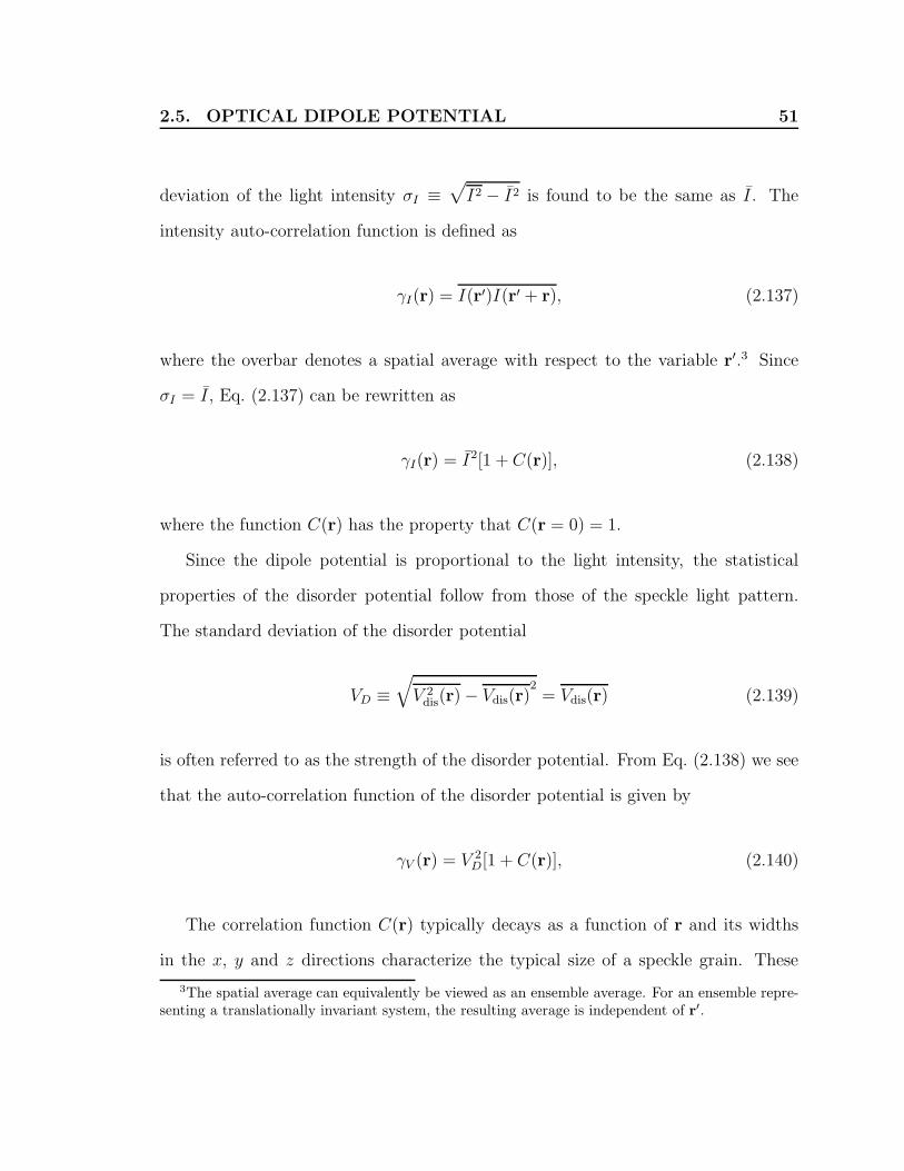


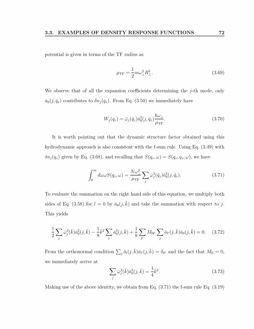
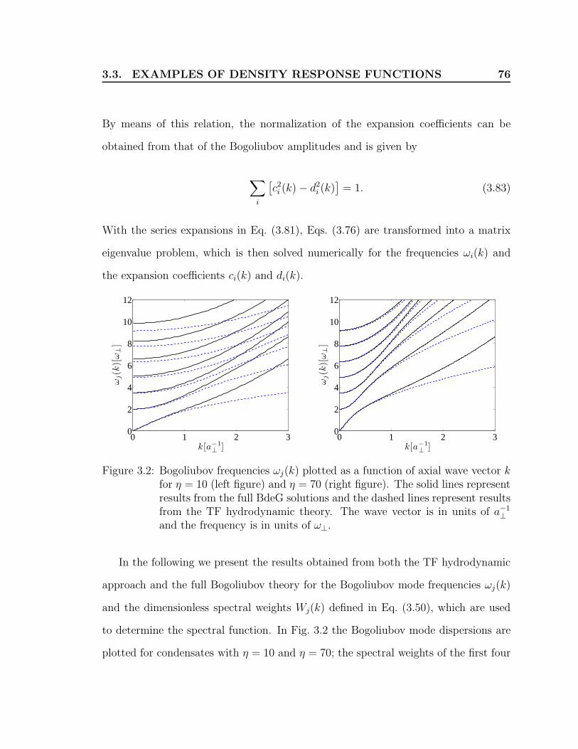

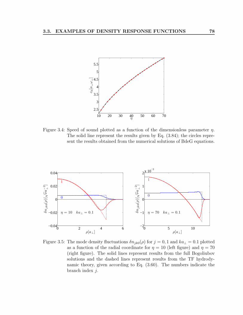
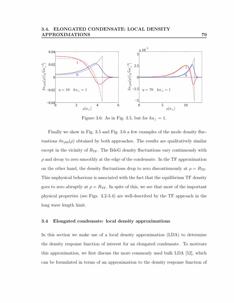


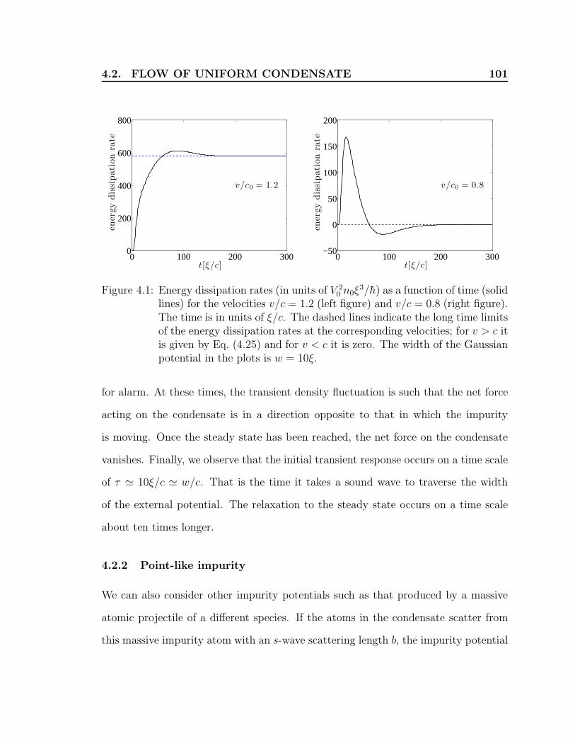
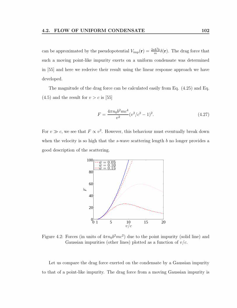


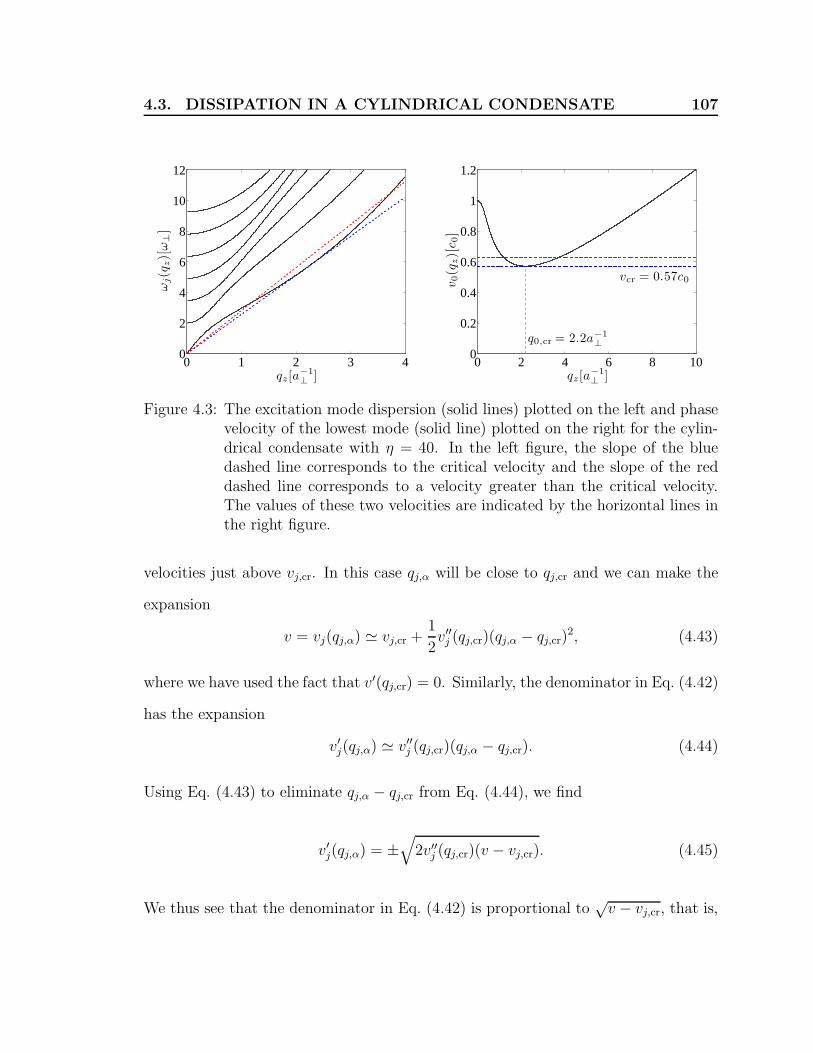

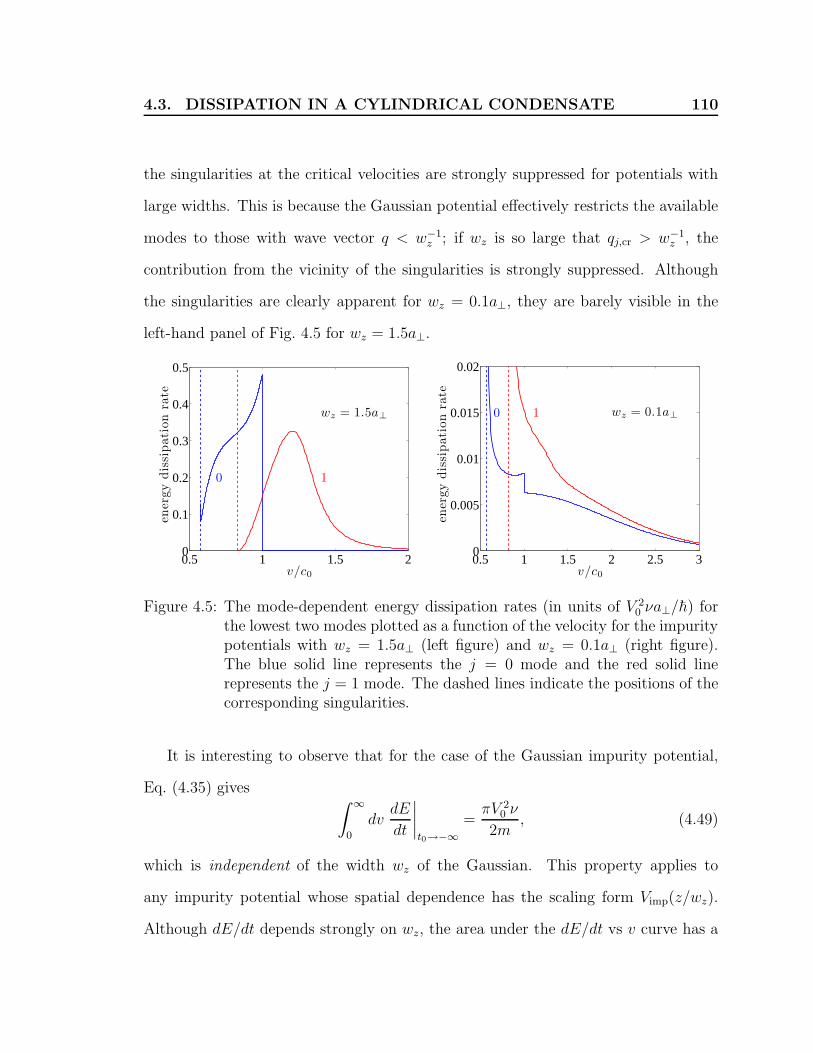


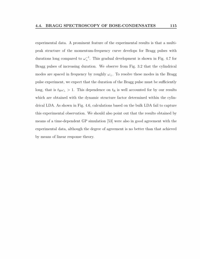


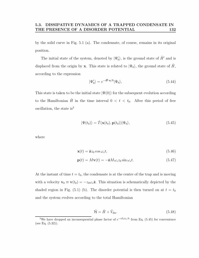
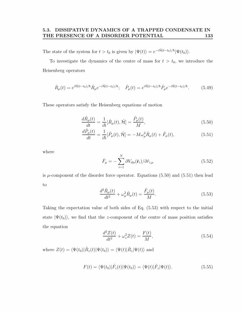
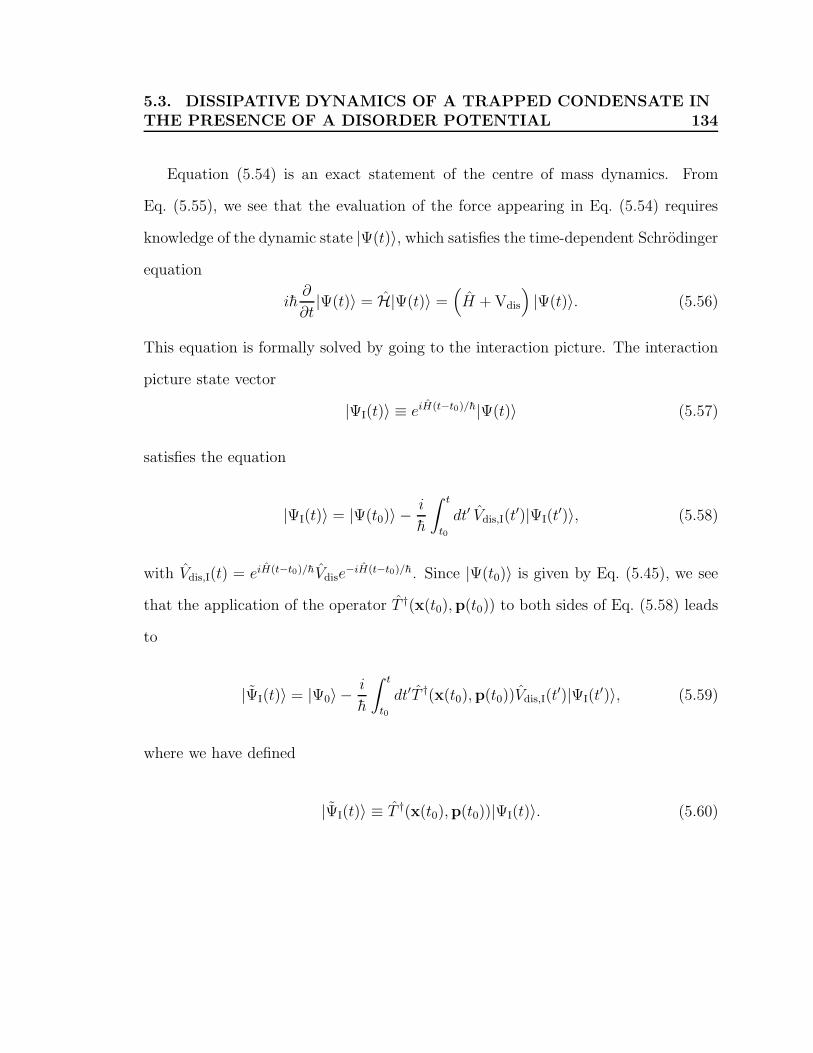
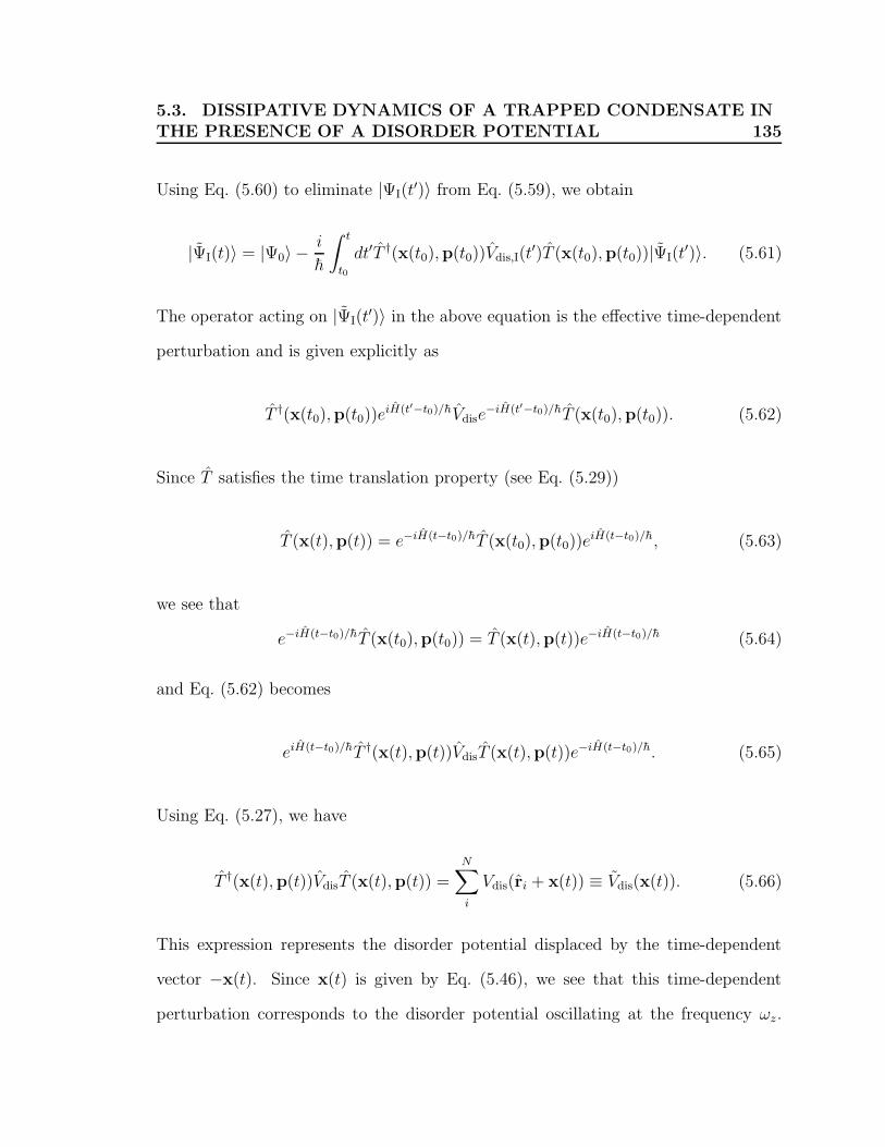


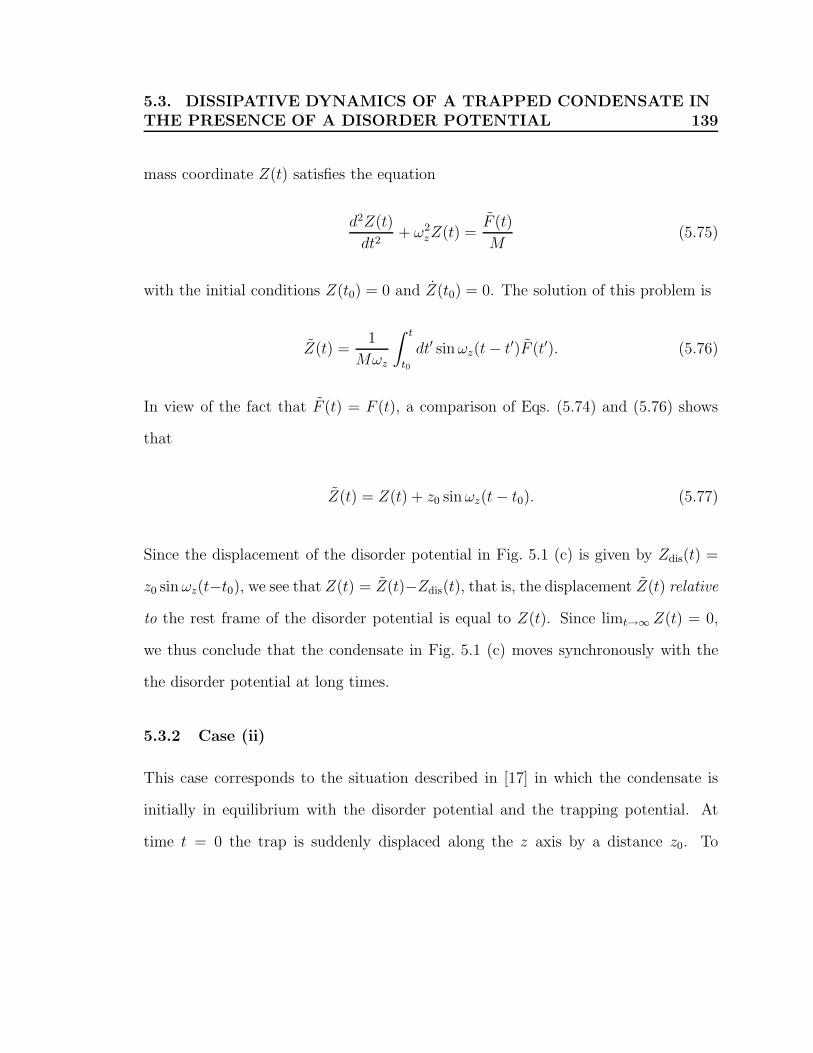
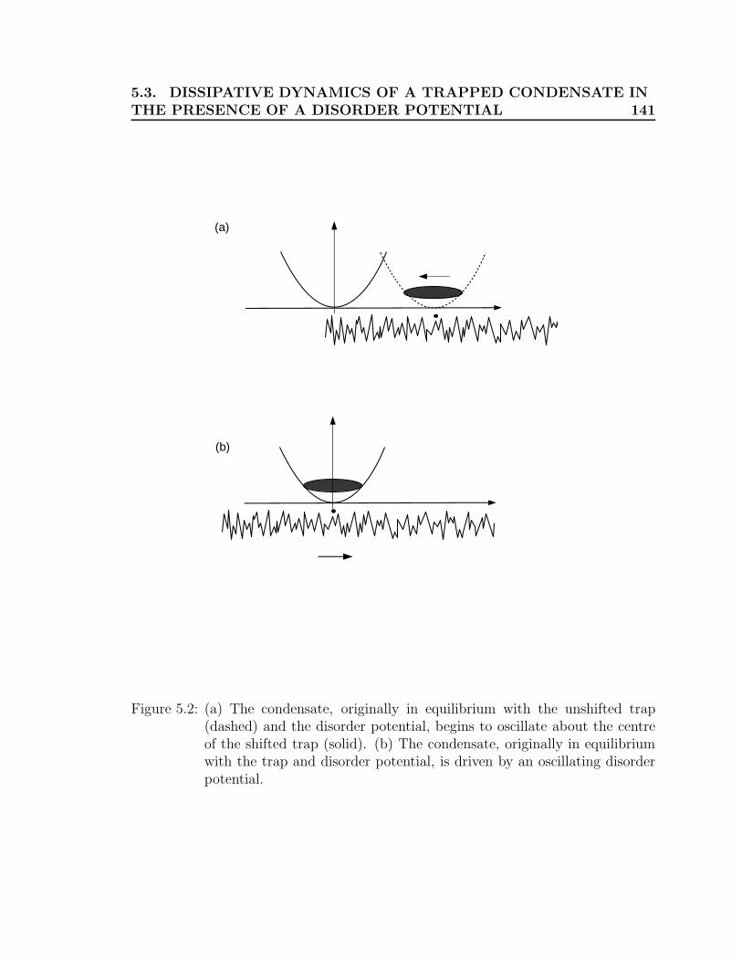
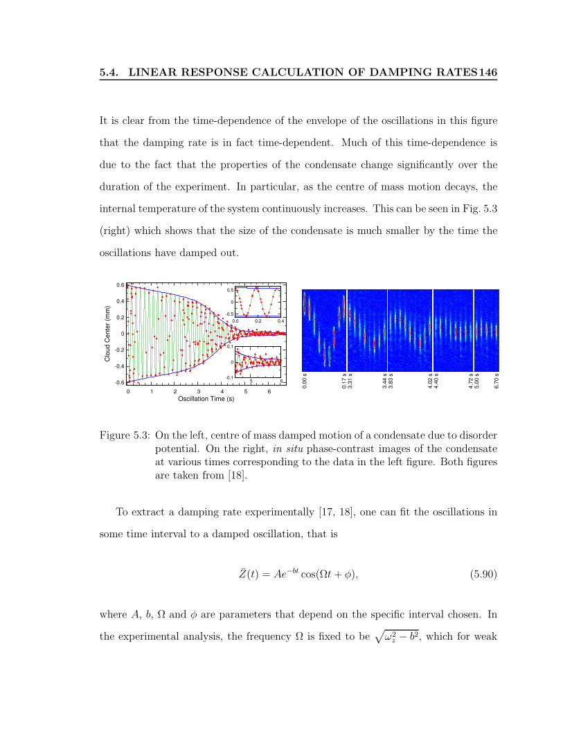


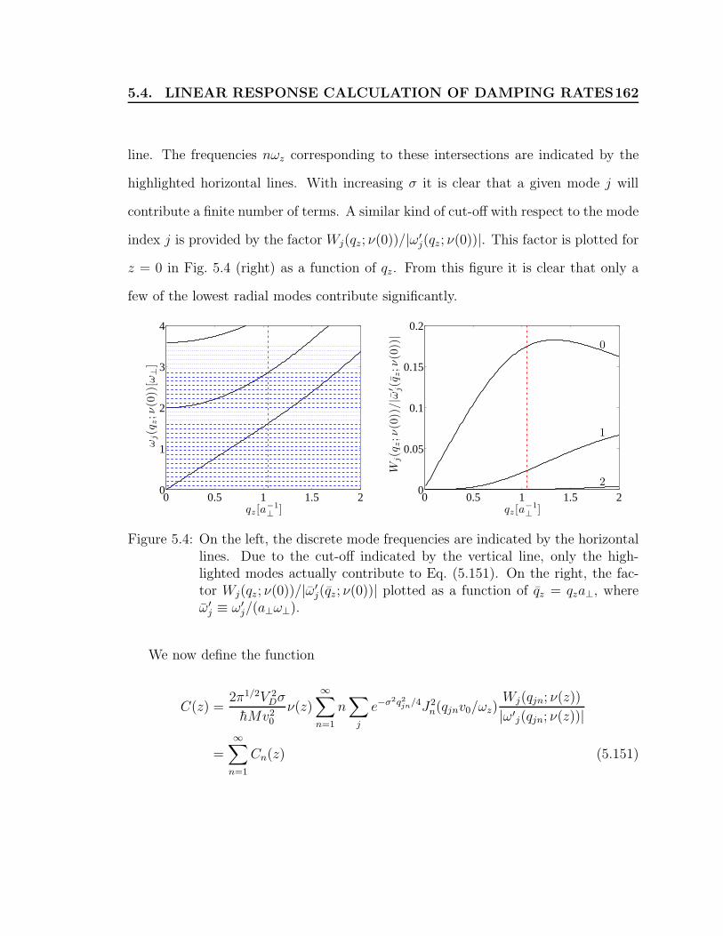
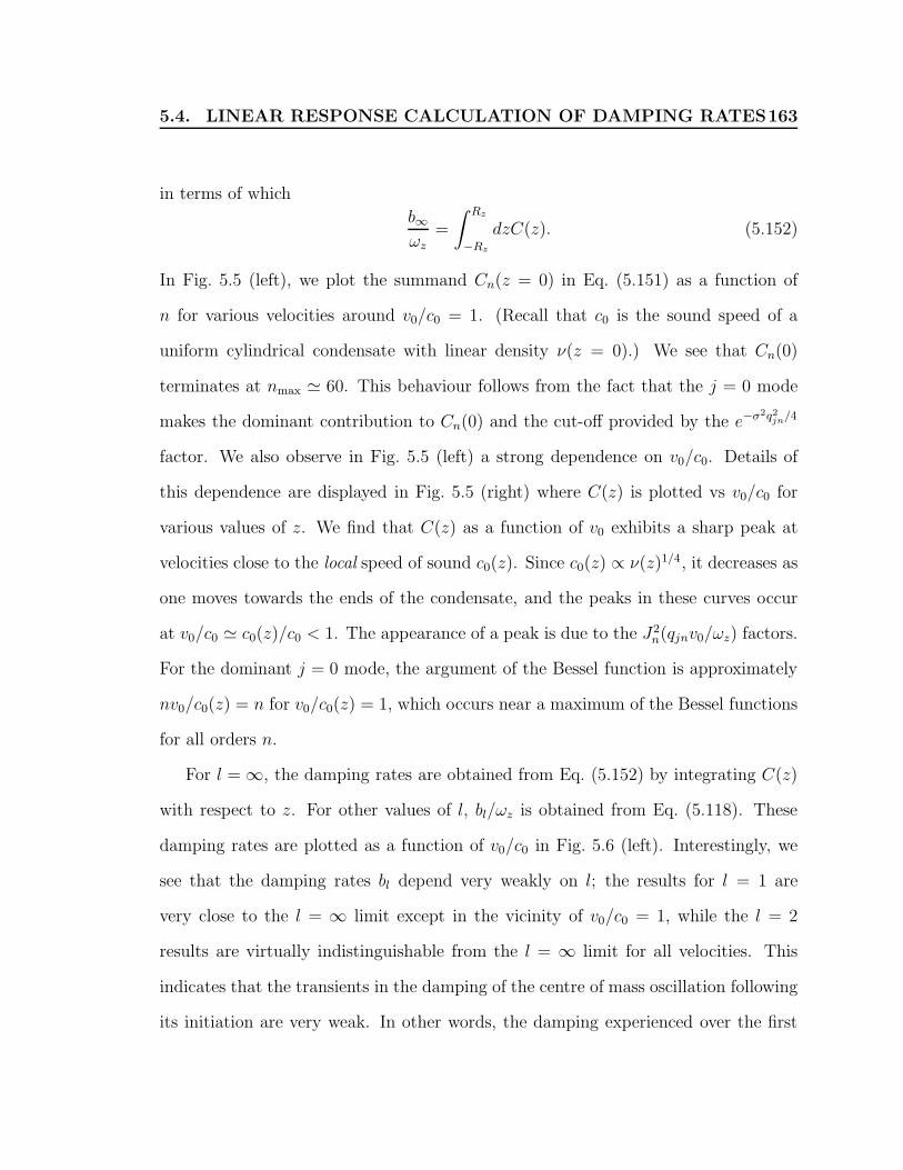

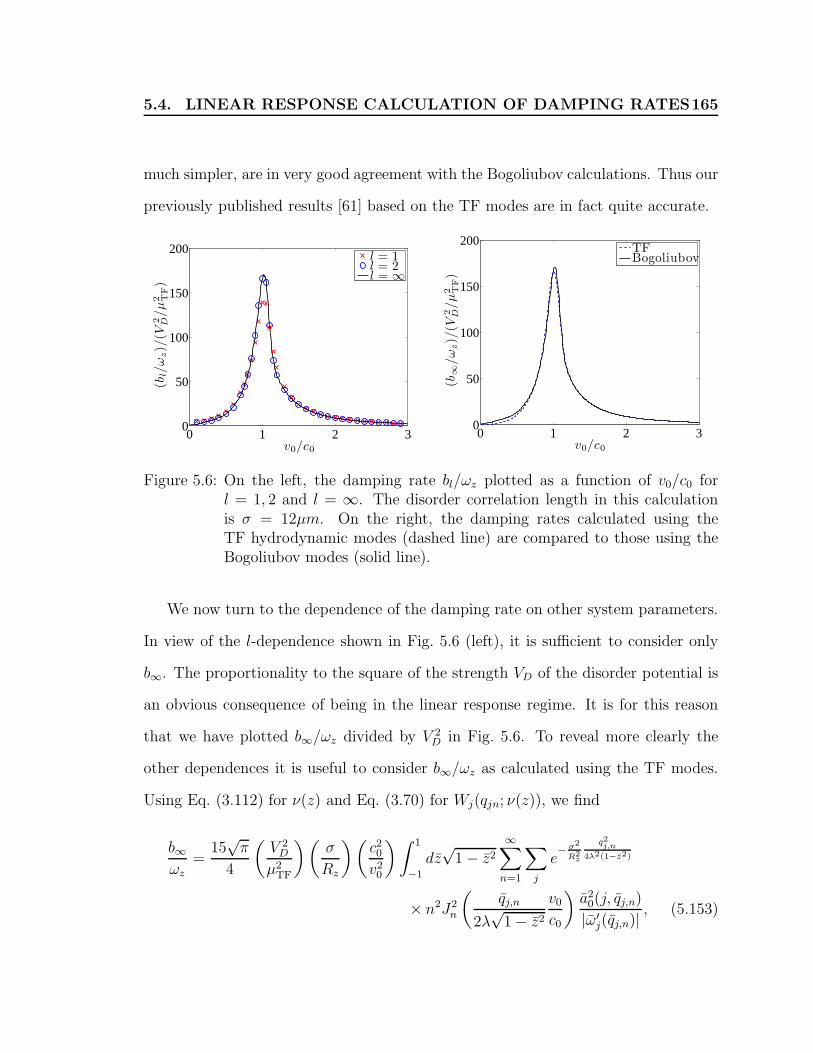

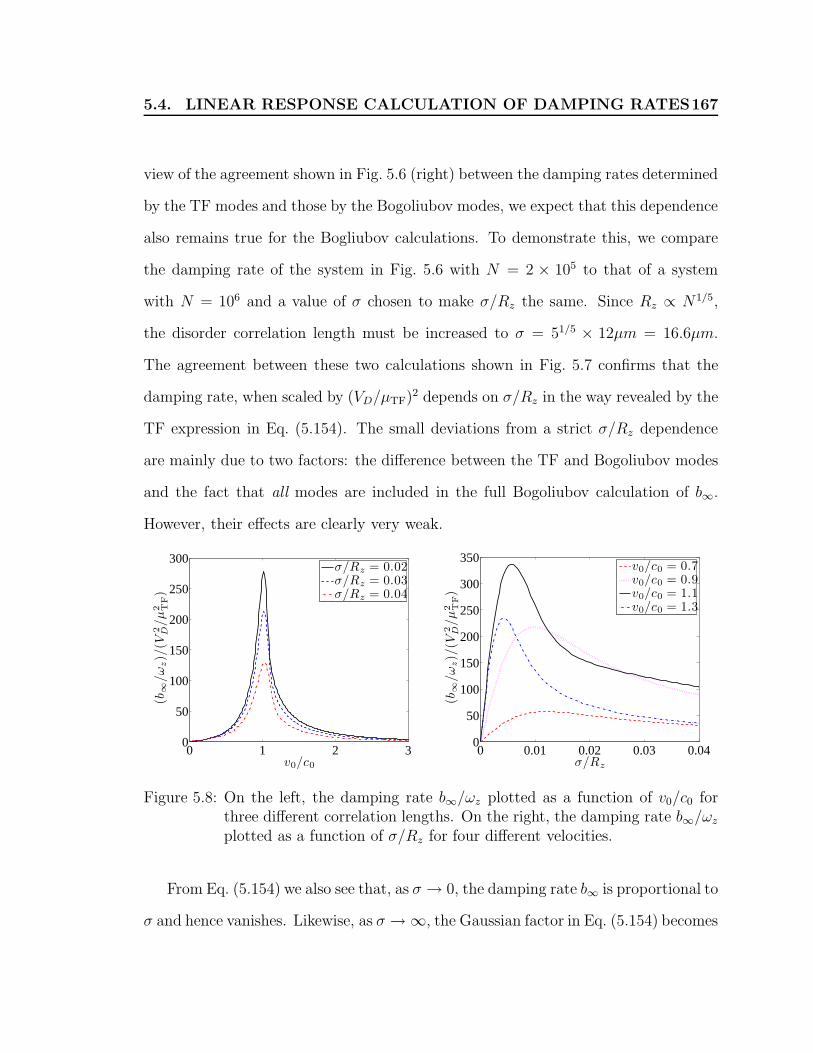

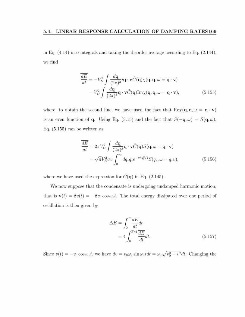
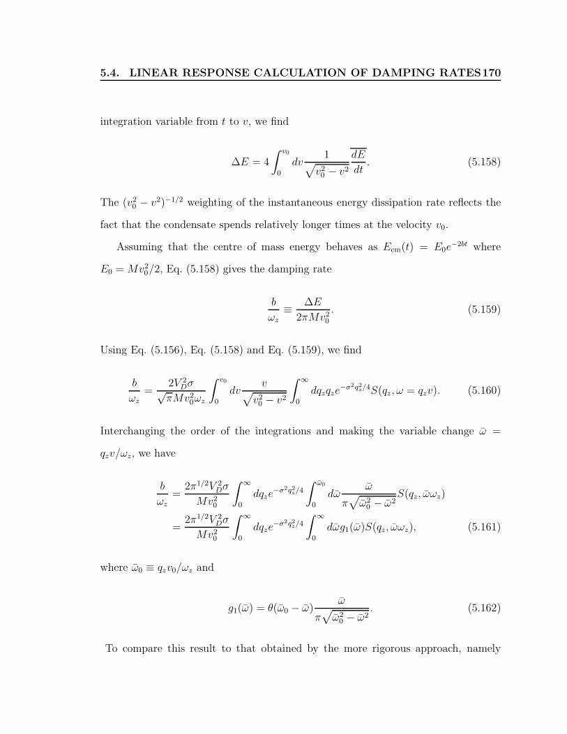

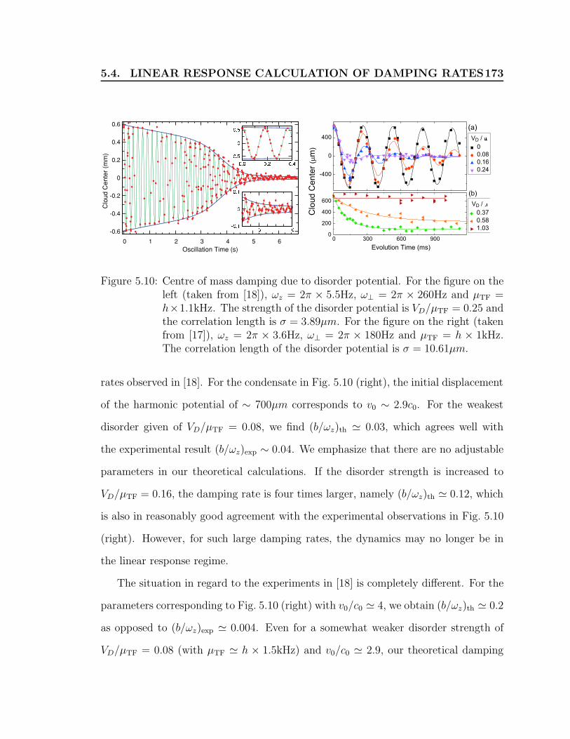

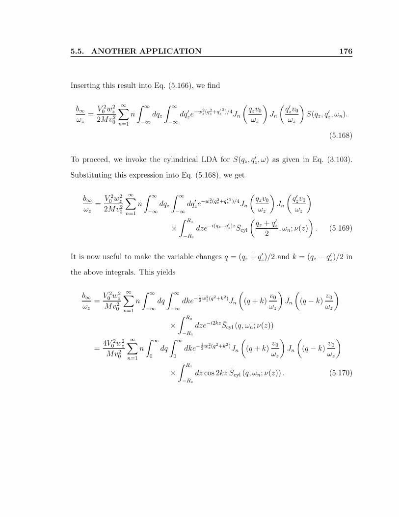

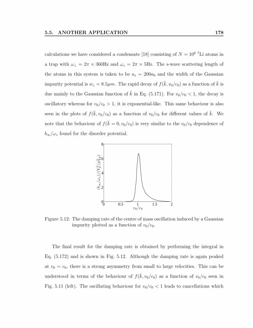
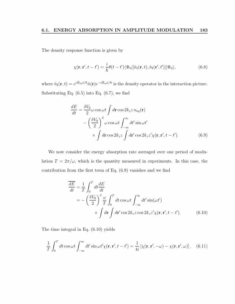

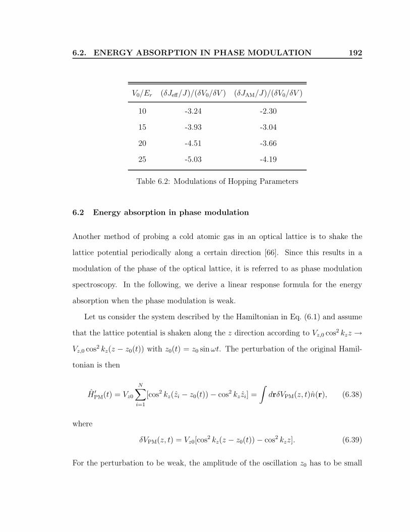
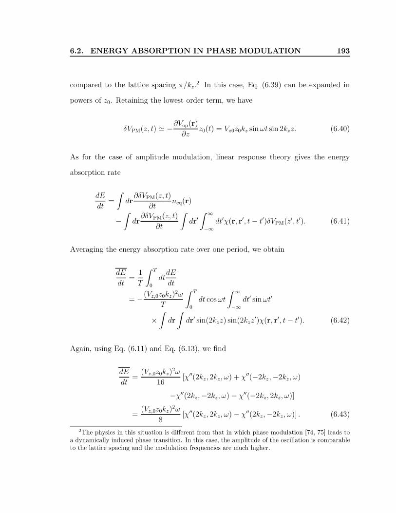


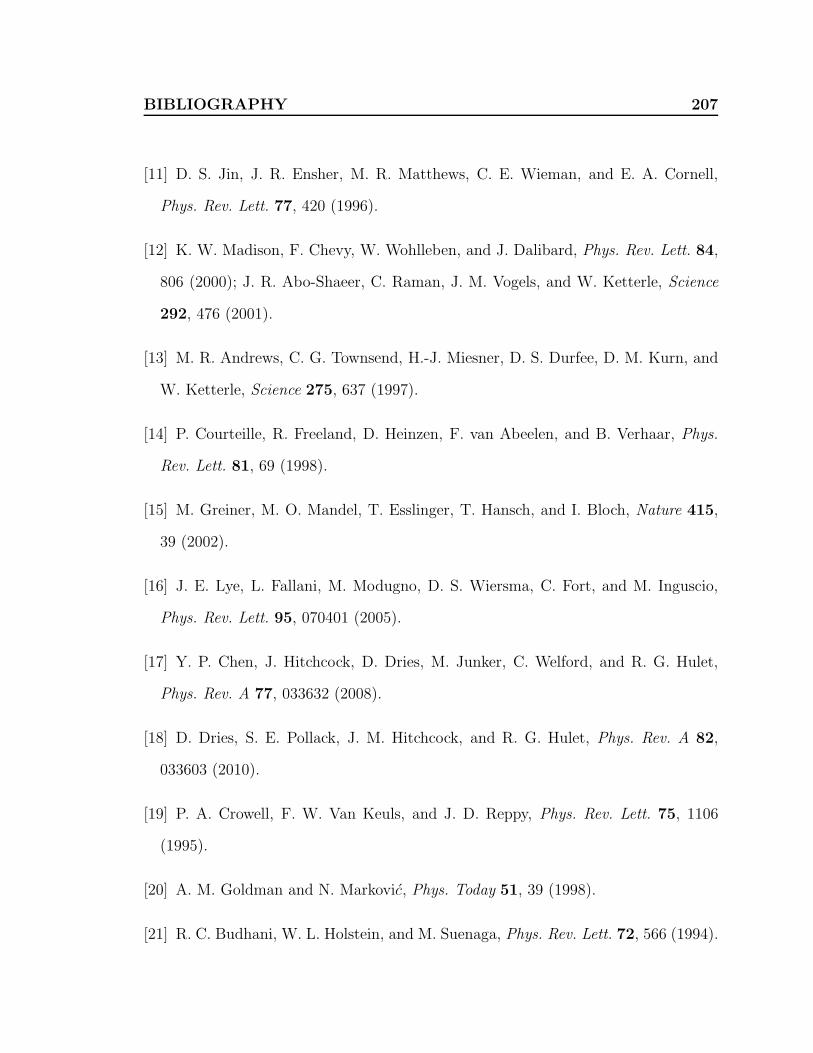
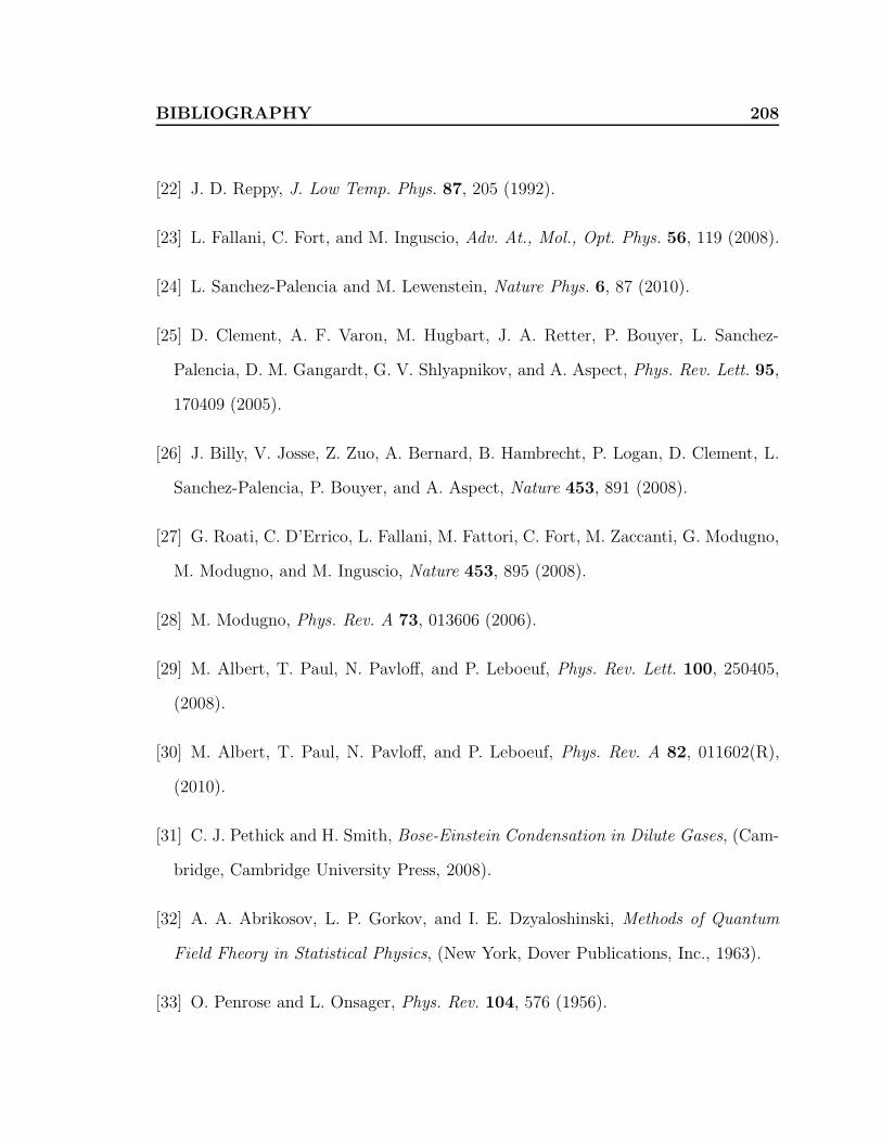


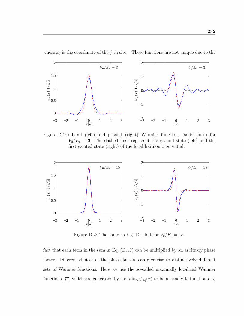


![Neutral impurities immersed in Bose{Einstein condensates€¦ · many-body quantum systems [1]. Notably, since the experimental realization of Bose{Einstein condensates (BEC) with](https://static.documents.pub/doc/80x56/5f0f02dc7e708231d4420bb4/neutral-impurities-immersed-in-boseeinstein-many-body-quantum-systems-1-notably.jpg)


