Distortion Risk Measures in Portfolio Optimization -...

Distortion Risk Measures in Portfolio Optimization

Ekaterina N. Sereda

HECTOR School of Engineering and ManagementUniversity of Karlsruhe

Efim M. Bronshtein

Professor of Ufa State Aviation Technical University

Svetozar T. Rachev

Chair-Professor, Chair of EconometricsStatistics and Mathematical Finance, School of Business Engineering

University of KarlsruheDepartment of Statistics and Applied Probability

University of California, Santa Barbaraand Chief Scientist FinAnalytica INC

Frank J. Fabozzi

Professor in the Practice of FinanceYale School of Management

Wei Sun

School of Economics and Business EngineeringUniversity of Karlsruhe

Stoyan Stoyanov

FinAnalytica INC., Seattle, USASchool of Business Engineering

University of Karlsruhe

1

1. Introduction

Abstract

Distortion risk measures are perspective risk measures because they allow anasset manager to reflect a client’s attitude toward risk by choosing the appropri-ate distortion function. In this paper, the idea of asymmetry was applied to thestandard construction of distortion risk measures. The new asymmetric distortionrisk measures are derived based on the quadratic distortion function with differentrisk-averse parameters.

Key words and phrases: risk measures, distortion risk measures, asymmetry, portfoliooptimization

1 Introduction

The selection of the appropriate portfolio risk measures continues to be a topic of heateddiscussion and intensive investigations in investment management, as all the proposedrisk measures have drawbacks and limited applications. The major focus of researchers1

has been on the “right” or “ideal” risk measure to be applied in portfolio selection. Theprincipal complexity, however, is that the concept of risk is highly subjective, becauseevery market player has its own perception of risk. Consequently, Balzer (2001) concludes,there is “no single universally acceptable risk measure.” He suggests the following featuresthat an investment risk measure should satisfy: relativity of risk, multidimensionality ofrisk, asymmetry of risk, and non-linearity.

Rachev et al. (2005) summarize the desirable properties of an “ideal” risk measure, cap-turing fully the preferences of investors. These properties relate to investment diversifica-tion, computational complexity, multi-parameter dependence, asymmetry, non-linearity,and incompleteness. However, every risk measure proposed in the literature possessesonly some of these properties. Consequently, proposed risk measures are insufficient and,based on this, Rachev et al. (2005, p. 4) conclude that an ideal measure does not exist.However, they note that “it is reasonable to search for risk measures which are ideal forthe particular problem under investigation.”

Historically, the most commonly used risk measure is the standard deviation (variance) ofa portfolio’s return. In spite of its computation simplicity, variance is not a satisfactorymeasure due to its symmetry property and inability to consider the risk of low probabilityevents.

A risk measure that has received greater acceptance in practice is value at risk (VaR).Unfortunately, because VaR fails to satisfy the sub-additivity property and ignores thepotential loss beyond the confidence level, researchers and practitioners2 have come torealize its limitations, limiting its use for reporting purposes when regulators require it orwhen a simple to interpret number is required by clients.

1See e.g. Goovaerts et al. (1984), Artzner et al. (1999), Kaas et al. (2001), Goovaerts et al. (2003),Zhang and Rachev (2004), Denuit et al. (2006), Rachev et al. (2005).

2See e.g. Arztner et al. (1999), Szego (2004), Zhang and Rachev (2004).

2

Sereda E., Bronshtein E., Rachev S., Fabozzi F., Sun W., and Stoyanov S.

A major step in the formulation of a systematic approach towards risk measures was takenby Artzner et al. (1999). They introduced the notion of “coherent” risk measures. Itturns out that VaR is not a coherent risk measure. In contrast, a commonly used riskmeasure in recent years, conditional value at risk (CVaR), developed by Rockafellar andUryasev (2002), is, in fact, a coherent risk measure. The most general theoretical resultabout coherent measures is the class of distortion risk measures, introduced by Denneberg(1990) and Wang et al. (1997).

Distortion risk measures were obtained by the simultaneous use of two approaches3 to de-fine the particular class of risk measures: axiomatic definition and the definition from theeconomic theory of choice under uncertainty. Due to the second approach, distortion riskmeasures have their roots in the dual utility theory of Yaari (1987). Using the expectedutility’s set of axioms with a modified independence axiom, Yaari (1987) developed thedistortion utility theory. He has shown that there must exist a “distortion function” suchthat a prospect is valued at its distorted expectation. Instead of using the tail probabili-ties in order to quantify risk, the decision maker uses the distorted tail probabilities. Forthe axiomatic definition, Wang et al. (1997) postulated the axioms to characterize theprice of insurance risk. These axioms include the following: law invariance, monotonicity,co-monotonic additivity, and continuity. They also proved that risk measures hold suchproperties if and only if they have the Choquet integral representation with respect to adistorted probability.

Distortion risk measures were originally applied to a wide variety of insurance prob-lems such as the determination of insurance premiums, capital requirement, and capitalallocation. Because insurance and investment risks are closely related, the investmentcommunity started to apply distortion risk measures in the context of the asset allocationproblem4. Wang (2004) has applied the distortion risk measure to price catastrophe bondsand Fabozzi and Tunaru (2008) to price real estate derivatives.

In the application of portfolio selection, distortion risk measures with the concave dis-tortion function reveal the desired properties, such as law-invariance, sub-additivity, andconsistency with second-order stochastic dominance. Law-invariance is the prerequisitefor the ability to quantify risk of a portfolio from historical data. Sub-additivity securesthe diversification effect. In general, the motif of constructing a portfolio is to reduceoverall investment risk through diversification as set forth by Markowitz (1952), that is,investing in different asset classes and in securities of many issuers. Diversification ensuresthe avoidance of extreme poor portfolio performance caused by the underperformance ofa single security or an industry. The consistency with second-order stochastic dominanceprovides the link between the construction of risk measures and the decision theory underuncertainty.

In this paper, we propose new distortion risk measures, adding the asymmetric property tothe already existing properties of concave distortion risk measures. We do so by extending

3The combination of two approaches – as demonstrated by Follmer and Schied (2002a), Tsanakas andDesli (2003), and Denuit et al. (2006) – add better perception of the inherent properties of risk measures.

4See, for example, van der Hoek and Sherris (2001), Gourieroux and Liu (2006), Hamada et al. (2006),and Balbas et al. (2007).

3

2. Classes of risk measures

the Choquet integral construction using quadratic and power distortion functions withdifferent concave parameters in order to better capture the risk perception of investors.

The paper is organized as follows. Section 2 starts with the general definition of risk andprovides various classifications of risk measures that have appeared in the literature. Sec-tions 3 and 4 provide a discussion of the distortion risk measures and their properties. InSection 5, we give examples of distortion functions and show how distortion risk measuresare related to VaR and CVaR. We propose the new distortion risk measures with asym-metric property in Section 6. Section 7 summarizes our paper. The appendix containsthe properties of risk measures and we make reference to them by property number in thebody of the paper.

2 Classes of risk measures

In general, a risk measure, ρ : X → R, is a functional that assigns a numerical value toa random variable representing an uncertain payoff. X is defined on L∞(Ω,F , P )5, thespace of all essentially bounded random variables defined on the general probability space(Ω,F , P ). Not every functional corresponds to the intuitive notion of risk. One of themain characteristics of such a function is that a higher uncertain return should conformto a higher functional value.

Goovaerts et al. (1984) presented the pioneering work of the axiomatic approach to riskmeasures in actuarial science, where risk measures were analyzed within the framework ofpremium principles. Artzner et al. (1999) extended the use of this axiomatic approach inthe financial literature. The axiomatic definition of how risk is measured includes the set-ting of the assorted properties (axioms) on a random variable and then the determinationof the mathematical functional fitting to the set of axioms.

2.1 Pederson and Satchell’s class of risk measures

Pederson and Satchell (1998) define risk as a deviation from a location measure. They pro-vided four desirable properties of a “good financial risk measure”, such as nonnegativity,positive homogeneity, sub-additivity, and translation invariance6. Pedersen and Satchellalso presented in their work the full characterization of the appropriate risk measuresaccording to their system of axioms.

5It could be efficient to use unbounded random variables for modeling risks, as far as financial riskhas no limits. The implications of risk measure’ properties can be different on certain finite and onnon-atomic probability spaces. Check Bauerle and Muller (2006) and Inoue (2003) for further results onthe extension from L∞ to L1 probability space.

6Property 8, property 2, property 3.1, and property 6.3, respectively.

4


2.2 Coherent risk measures

The idea of coherent risk measures was introduced by Artzner et al. (1999). Coherent riskmeasures are those measures which are translation invariant, monotonous, sub-additive,and positively homogeneous7. Coherent measures have the following general form:

ρ(X) = supQ∈Q

EQ[−X],

where Q is some class of probability measures on Ω.

Four criteria proposed by Artzner et al. (1999) provide rules for selecting and evaluatingrisk measures. However, one should be aware that not all risk measures satisfying thefour proposed axioms are reasonable to use under certain practical situations. Wang(2002) argued that “a risk measure should go beyond coherence” in order to utilize usefulinformation in a large part of a loss distribution. Dhaene et al. (2003), observing “bestpractice” rules in insurance, concluded that coherent risk measures “lead to problems”.

2.3 Convex risk measures

Convex risk measures (also called weakly coherent risk measures) were studied by Follmerand Schied (2002a, 2002b) and Frittelli and Rosazza Gianin (2005). Convex risk measuresare a generalization of coherent risk measures obtained by relaxation of the positive ho-mogeneity assumption (property 2) together with the sub-additivity condition (property3.1) and require the weaker property of convexity (property 4). Any convex risk measuretakes into account a nonlinear increase of the risk with the size of the position and hasthe following structure:

ρ(X) = supQ∈Q

(EQ[−X] − α(Q)) ,

where α is a penalty function defined on probability measures on Ω.

Following Frittelli and Rosazza Gianin (2005), a functional ρ : X → R is a convex riskmeasure if it suffices convexity (property 4), lower semi-continuity (property 9.5), andnormalization (ρ(0) = 0) conditions. Bauerle and Muller (2006) proposed replacing theconvexity axiom by the weaker but more intuitive property of consistency with respect toconvex order (property 7.6).

2.4 Law invariant coherent risk measures

Following the notation of Kusuoka (2001), law invariant coherent risk measures have theform:

ρα(X)∆=

1

α

∫ 1

1−α

Z−X(x) dx,

7Property 6.3, property 5, property 3.1, and property 2, respectively.

5


Z : [0, 1) → R is non-decreasing and right continuous. This class of risk measures satisfiesthe lower semi-continuity property (property 9.5) for all X ∈ L∞, 0 ≤ α ≤ 1. The classof insurance prices characterized by Wang et al. (1997) is an example of law invariantcoherent risk measures.

2.5 Spectral risk measures

Spectral measures of risk8 can be defined by adding two axioms to the set of coherencyaxioms: law invariance (property 1) and comonotonic additivity (property 3.2). Spectralrisk measures consist of a weighted average of the quantiles of the returns distributionusing a non-increasing weight function9 referred to as a spectrum and denoted by φ. It isdefined as follows:

Mφ(X) = −∫ 1

0

φ(x)F←−X

(x) dx,

where φ is a non-negative, non-increasing, right-continuous integrable function defined on[0, 1] and such that

∫ 1

0φ(x) dx = 1. Assumptions made on φ determine the coherency of

spectral risk measures. If any of these assumptions is relaxed, the measure is no longercoherent. Spectral risk measures possess positive homogeneity (property 2), translationinvariance (property 6.3), monotonicity (property 5), sub-additivity (property 3.1), lawinvariance (property 1), comonotonic additivity (property 3.2), consistency with second-order stochastic dominance (SSD) (property 7.4), and expected utility theory.

2.6 Deviation measures

Rockafeller et al. (2002)10 defined deviation measures as positive, sub-additive, positivelyhomogeneous, Gaivoronsky-Pflug (G-P) translation invariant11 risk measures. Deviationmeasures are normally used by the totally risk-averse investors.

2.7 Expectation-bounded risk measures

Rockafeller et al. (2002) proposed expectation-bounded risk measures, imposing the con-ditions of sub-additivity, positive homogeneity, translation invariance and additional prop-erty of expectation-boundedness12. There exists a corresponding one-to-one relationshipbetween deviation measures and expectation-bounded risk measures. One can deriveexpectation-bounded coherent risk measures if additionally monotonicity (property 5) issatisfied.

8See Kusuoka (2001), Acerbi (2002), Adam et al. (2007).9φ can be observed as a weight function reflecting an investor’s subjective risk aversion.

10See also Rockafeller et al. (2003, 2006).11Property 8, property 3.1, property 2, and property 6.2, respectively.12Property 3.1, property 2, property 6.3, and property 10, respectively.

6


2.8 Reward measures

De Giorgi (2005) introduced the first axiomatic definition for reward measures and pro-vided their characterization. According to de Giorgi, such measures should satisfy thefollowing conditions: additivity, positive homogeneity, isotonicity with respect to SSD,and risk-free condition13.

2.9 Parametric classes of risk measures

Stone (1973) defined a general three-parameter class of risk measures, which has the form

R[c, k, A] =

(∫ −∞

A

|y − c|kf(y) dy

)1/k

,

where A, c ∈ R and k > 0. Stone’s class of risk measures includes several commonlyused measures of risk and dispersion, such as the standard deviation, the semi-standarddeviation, and the mean absolute deviation.

Pedersen and Satchell (1998) generalized Stone’s class of risk measures and introducedthe five-parameter class of risk measures:

R[A, c, α, θ, w(·)] =

[∫ −∞

A

|y − c|αw [F (y)] f(y)dy

]θ

for some bounded function w(·), A, c ∈ R, α > 0, θ > 0. This class of risk measures alsoinclude the lower partial moments as an extention of the Stone class. Ebert (2005) arguesthat because of the confusing number of parameters presented by Pedersen and Satchell,“it seems to be impossible to comprehend their meaning and their interaction”.

2.10 Quantile-based risk measures

Quantile-based risk measures include value at risk, expected shortfall, tail conditionalexpectation, and worst conditional expectation. We describe each measure below.

Value at risk (VaR) specifies how much one can lose with a given probability (confidencelevel). Its formal definition is

V aRα(X) = −x(α) = q1−α(−X).

VaR has the following properties: monotonicity (property 5), positive homogeneity (prop-erty 2), translation invariance (property 6.3), law invariance (property 1), comonotonicadditivity (property 3.2). VaR possesses the sub-additivity attribute (property 3.1) forjoint-elliptically distributed risks (see Embrechts et al. (2002)), but this assumption israre in practice.

13Property 3.2, property 2, property 7.4, and property 13.2, respectively.

7


Despite its simplicity and wide applicability, VaR is controversial. A common criticismamong academics is that VaR is not sub-additive, hence not coherent and that VaRcalculations lead to substantial estimation errors (see e.g. Arztner et al. (1999), Szego(2004), and Zhang and Rachev (2004)). A risk manager should be aware of its limitationsand use it properly.

Expected shortfall (ES), also known as tail (or conditional) VaR (see Rockafellar et al.(2002)), corresponds to the average of all V aRαs above the threshold α:

ESα(X) =1

1 − α

∫ 1

α

V aRu(X) du, α ∈ (0, 1).

ES was proposed in order to overcome some of the theoretical weaknesses of VaR. ES hasthe following properties: law invariance (property 1), translation invariance (property6.3), comonotonic additive (property 3.2), continuity (property 9), monotonicity (prop-erty 5), sub-additivy (property 3.1). ES, being coherent14, was proposed by Artzner etal. (1999) as a “good” risk measure.

Tail conditional expectation (TCE) was proposed by Artzner et al. (1999) in the followingform:

TCEα(X) = −EX|X ≤ x(α),TCEα does not possess the sub-additivity property for general distributions; it is coherentonly for continuous distributions.

Worst conditional expectation (WCE) is defined as

WCEα(X) = − infE[X|A] : A ∈ F , P (A) > α.

WCEα(X) is not law-invariant, so it cannot be estimated solely from data. Using suchmeasures can lead to different risk values for two portfolios with identical loss distributions.

Comparing ES, TCE, and WCE, one finds that

TCEα(X) ≤ WCEα(X) ≤ ESα(X).

ES has the maximum value among TCE and WCE when the underlying probability lawvaries. If the distribution of X is continuous, then

TCEα(X) = WCEα(X) = ESα(X).

2.11 Drawdown measures

Drawdown measures are intuitive measures. A psychological issue in handling risk is thetendency of people to compare the current situation with the very best one from the past.Drawdowns measure the difference between two observable quantities - local maximumand local minimum of the portfolio wealth. Cheklov et al. (2003) defined the drawdown

14See Acerbi and Tasche (2004).

8


function as the difference between the maximum of the total portfolio return up to timet and the portfolio value at t.

Drawdown measures are close to the notion of deviation measure. Examples of draw-down measures constitute absolute drawdown (AD), maximum drawdown (MDD), av-erage drawdown (AvDD), drawdown at risk (DaR), and conditional drawdown at risk(CDaR). In spite of their computational simplicity, drawdown measures cannot describethe real situation on the market, and therefore, should be used in combination with othermeasures.

3 Distortion risk measures

A distortion risk measure can be defined as the distorted expectation of any non-negativeloss random variable X. It is accomplished by using a “dual utility” or the distortionfunction g15 as follows:

ρg(X) =

∫ ∞

0

g(1 − FX(x)) dx =

∫ 1

0

F−1X (x)(1 − q) dg(q), (1)

where g : [0, 1] → [0, 1] is a continuous increasing function with g(0) = 0 and g(1) = 1;FX(x) denotes the cumulative distribution function of X, while g(FX(x)) is referred to asa distorted distribution function.

For the gain/loss-distributions, when the loss random variable can take any real number,the distortion risk measure is obtained as follows:

ρg(X) =

∫ 1

0

F−1X (x)dH(x) = −

∫ 0

−∞

H(FX(x))dx +

∫ ∞

0

[1 − H(FX(x))]dx,

where H(u) = 1 − g(1 − u). A similar expression holds if we use the survival functionSX(x) = 1 − FX(x) = P (X > x) instead of the distribution function,

ρg(X) = −∫ 0

−∞

[1 − g(SX(x))]dx +

∫ ∞

0

g(SX(x))dx.

Van der Hoek and Sherris (2001) developed a more general class of distortion risk mea-sures, depending on the choice of parameters α, g, and h. It has the following form:

Hα,g,h(X) = α + Hh

(

(X − α)+)

− Hg

(

(α − X)+)

,

where α+ = max[0, α]. When α = 0 and h(x) = 1 − g(1 − x), then we again obtain theChoquet integral representation.

15Consider the set function g : F → [0,∞), defined on the σ-algebra F , such that g(∅) = 0 and A ⊆ B

⇒ g(P [A]) ≤ g(P [B]), for A,B ∈ F . Such a function g is called a distortion function, and P [A], P [B] –distorted probabilitites.

9

4. Properties of distortion risk measures

4 Properties of distortion risk measures

The properties of the distortion risk measures correspond to the following standard resultsabout the Choquet integral (see Denneberg (1994)):

1. If X ≥ 0, then ρg(X) ≥ 0, monotonicity

2. ρg(λX) = λρg(X), for all λ ≥ 0, positive homogeneity

3. ρg(X + c) = ρg(X) + c, for all c ∈ R, translation invariance16

4. ρg(−X) = −ρg(X), where g(x) = 1 − g(1 − x)17

5. If a random variable Xn has a finite number of values (i.e., Xnw→ X) and ρg(X)

exists, then ρg(Xn) → ρg(X). This property implies that it is enough to prove thestatement for the discrete random variables, and then carry over the result to thegeneral continuous case.

6. If X and Y are comonotonic risks, taking positive and negative values, then

ρg(X + Y ) = ρg(X) + ρg(Y )

In literature, this property is called comonotonic additivity.

16The proof is as follows:

ρg(X + c) =

∫

−∞

0

[g(SX+c(x) − 1] dx +

∫ c

0

g(SX+c(x)) dx +

∫

∞

c

g(SX+c(x)) dx

=

∫ 0

−∞

[g(SX(x − c)) − 1] dx +

∫ c

0

g(SX(x − c)) dx +

∫

∞

c

g(SX(x − c)) dx.

By replacing x = c + u, we get

ρg(X + c) =

∫

−c

−∞

[g(SX(u)) − 1] du +

∫ 0

−c

g(SX(u)) du +

∫

∞

0

g(SX(u)) du

=

∫ 0

−∞

[g(SX(u)) − 1] du +

∫

∞

0

g(SX(u)) du +

∫ 0

−c

du

= ρg(X) + c.

17The proof is as follows:

ρg(−X) =

∫

−∞

0

[g(S−X(x) − 1] dx +

∫

∞

0

g(S−X(x)) dx

=

∫ u

−∞

[g(1 − SX(−x) + P [X = x]) − 1] dx +

∫ u

−∞

g(1 − SX(−x) + P [X = x]) dx

=

∫ u

−∞

(g(1 − SX(−x)) − 1) dx +

∫ u

−∞

g(1 − SX(−x)) dx.

Replacing x by −u, we get

ρg(−X) = −∫ u

−∞

(g(1 − SX(u)) − 1) du −∫ u

−∞

g(1 − SX(u)) du = −ρg(X).

10


7. In the generalized case, distortion risk measures are not additive18:

ρg(X + Y ) 6= ρg(X) + ρg(Y )

8. Distortion risk measures are sub-additive if and only if the distortion function g(x)is concave.

ρg(X + Y ) ≤ ρg(X) + ρg(Y )

The proof is given in Wirch and Hardy (1999). Hence, concave distortion riskmeasures are coherent risk measures.

9. For a non-decreasing distortion function g, the associated risk measure ρg is consis-tent with the stochastic dominance of order 1

X ≤1 Y ⇒ ρg(X) ≤ ρg(Y )

The proof is given in Hardy and Wirch (2003).

10. For a non-decreasing concave distortion function g, the associated risk measure ρg

is consistent with the stochastic dominance of order 2 (i.e., SSD)

X ≤2 Y ⇒ ρg(X) ≤ ρg(Y ).

As a result, every coherent distortion risk measure is consistent with respect tosecond-order stochastic dominance.

11. For a strictly concave distortion function g, the associated risk measure ρg is strictlyconsistent with the stochastic dominance of order 2

X <2 Y ⇒ ρg(X) < ρg(Y )

The proof is given in Hardy and Wirch (2003).

12. Consistency of distortion risk measures with respect to the higher-order stochasticdominances was analyzed in the financial and actuarial literature. In particular,Hurlimann (2004) obtained some results about the consistency of distortion riskmeasures with stochastic dominance of order 3. The necessary precondition to thatis the consistency with respect to 3-convex order. The only distortion risk measureswhich are consistent with 3-convex order are g(x) =

√x and g(x) = x under the

assumption that the set of possible losses contains all Pareto19 variables (Theorem6.3 in Hurlimann (2004)). Under a much weaker hypothesis of discrete losses, Belliniand Caperdoni (2006) showed that the only coherent distortion risk measure that isconsistent with respect to the 3-convex order is the expected value, when g(x) = x,leaving the problem open for the case of continuous losses.

18The proof is as follows. Consider the function g = x2, the joint distribution of discrete randomvariables X and Y is defined as follows: P (1, 1) = P (−1, 1) = P (1,−1) = P (−1,−1) = 0.25. Themarginal distributions X and Y have the forms: P (1) = P (−1) = 0.5. Direct calculations show that

ρg(X) = ρg(Y ) = −0.5; ρg(X + Y ) = 0.25; 0.25 6= −1

The risks X and Y are independent here.19With a generic location and scale parameter allowed.

11

5. Examples of distortion risk measures

5 Examples of distortion risk measures

As explained above, the choice of distortion function specifies the distortion risk measures.Thus, finding “good” distorted risk measures boils down to the choice of a “good” dis-tortion function. The properties one might use as a criteria for the choice of a distortionfunction include continuity, concavity, and differentiability. Many different distortionsg have been proposed in the literature. Some well-known ones are presented below. Asummary of other proposed distortion functions can be found in Denuit et al. (2005).

With g(x) = x, we have ρg(X) = E[X], if the mathematical expectation exists20.

VaR corresponds to the distortion:

g(x) =

0, if x < 1 − p;

1, if x ≥ 1 − p.

The distortion function is discontinuous in this case due to the jump at x = 1 − p(see Figure 1). This predetermines that VaR is not coherent. As a result, VaR doesnot represent a “good” behaved distortion function.

CVaR can be defined as a distortion risk measure based on the distortion function

g(x) = min

(

x

1 − p, 1

)

, x ∈ [0, 1]

Figure 2 presents the given function. It is continuous, implying that CVaR is co-herent. But the distortion function of CVaR is not differentiable at x = 1 − p.Consequently, it discards potentially valuable information because it maps all per-centiles below (1−p) to a single point “0”. By doing so, it fails to take into accountthe severity of extreme values (Wang (2002)).

In order to overcome these sorts of problems, Wang (2002) considers the followingspecification of g:

g(x) = Φ(

Φ−1(x) − Φ−1(q))

,

20We limit our proof to the interval [−a, a]. In this case the mathematical expectation accurately exists.

ρg(X) =

∫

−a

0

(SX(x) − 1) dx +

∫ 0

a

SX(x) dx

= −∫ 0

−a

FX(x) dx +

∫ a

0

(1 − FX(x)) dx

= a −∫ a

−a

FX(x) dx

By integrating by parts, we get

ρg(X) = a − xFX(x)|a−a +

∫ a

−a

x dFX(x) = E[X],

as FX(a) = 1, FX(−a) = 0. In this particular case, the distortion risk measures are additive.

12


Figure 1. Distortion function of VaR

Figure 2. Distortion function of CVaR

13

6. New distortion risk measures

for p ∈ [0, 1], where 0 < q ≤ 0.5 is some parameter21. The distortion functiong is indeed non-decreasing, concave, and such that g(0) = 0 and g(1) = 1. Thecorresponding risk measure WTq is known as the Wang transform. The parameterq can be changed to make the Wang transform either sharper on high losses orsofter and more receptive to positive returns. Wang (2002) recommended the Wangtransform for the measurement of insurance risks.

The beta family of distortion risk measures, proposed by Wirch and Hardy (1999),utilizes the incomplete beta function:

g(FX(x)) = β(a, b; FX(x)) =

∫ FX(x)

0

1

β(a, b)ta−1(1 − t)b−1 dt = Sβ(FX(x))

where Sβ(x) is the distribution function of the beta distribution, and β(a, b) is thebeta function with parameters a > 0 and b > 0, that is

β(a, b) =Γ(a)Γ(b)

Γ(a + b)=

∫ 1

0

ta−1(1 − t)b−1 dt.

The beta-distortion risk measures are concave if and only if a ≤ 1 and b ≥ 1; strictlyconcave if a and b are both not equal to 1.

The Proportional Hazard (PH) transform is a special case of the beta-distortionrisk measure with a = 0.1, b = 1. The PH-transform risk measure is defined as:

ρPH(X) =

∫ ∞

0

SX(x)1

γ dx, γ > 1,

where SX(x) = 1 − FX(x).

6 New distortion risk measures

The notion of asymmetry of the risk perception of investors was studied in the classicalworks such as Kahneman and Tversky (1979). Here we apply the idea of asymmetry tothe standard construction of the distortion risk measures. Introducing the asymmetryinto the Choquet integral, we obtain the following distortion risk measures:

ρgi(X) = −

∫ 0

−∞

[1 − g1(SX(x))] dx +

∫ ∞

0

g2(SX(x)) dx,

where distortion functions g1 and g2 only differ by their risk-averse parameters.

Moreover, the risk-averse parameter should be inserted in the properly chosen distortionfunction. Here we propose the quadratic distortion function

gi(x) = x + ki(x − x2),

21We need q ≤ 0.5 in order to get concave distortion risk measures.

14


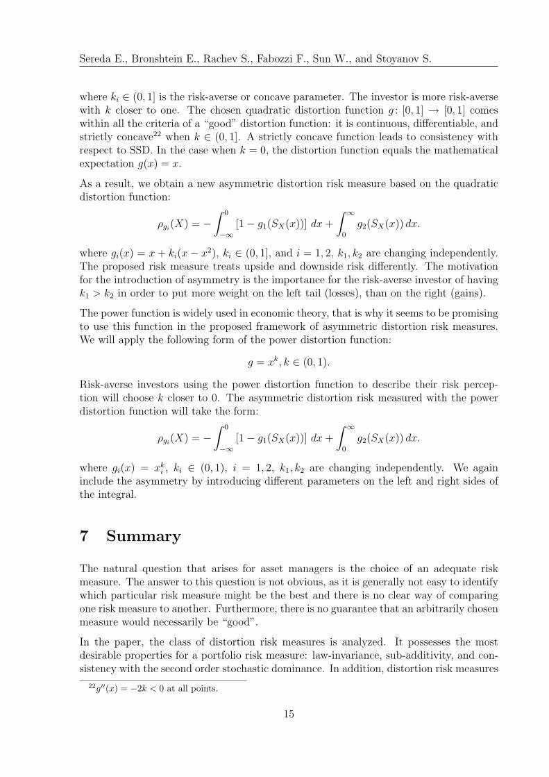
where ki ∈ (0, 1] is the risk-averse or concave parameter. The investor is more risk-aversewith k closer to one. The chosen quadratic distortion function g : [0, 1] → [0, 1] comeswithin all the criteria of a “good” distortion function: it is continuous, differentiable, andstrictly concave22 when k ∈ (0, 1]. A strictly concave function leads to consistency withrespect to SSD. In the case when k = 0, the distortion function equals the mathematicalexpectation g(x) = x.

As a result, we obtain a new asymmetric distortion risk measure based on the quadraticdistortion function:

ρgi(X) = −

∫ 0

−∞

[1 − g1(SX(x))] dx +

∫ ∞

0

g2(SX(x)) dx.

where gi(x) = x + ki(x − x2), ki ∈ (0, 1], and i = 1, 2, k1, k2 are changing independently.The proposed risk measure treats upside and downside risk differently. The motivationfor the introduction of asymmetry is the importance for the risk-averse investor of havingk1 > k2 in order to put more weight on the left tail (losses), than on the right (gains).

The power function is widely used in economic theory, that is why it seems to be promisingto use this function in the proposed framework of asymmetric distortion risk measures.We will apply the following form of the power distortion function:

g = xk, k ∈ (0, 1).

Risk-averse investors using the power distortion function to describe their risk percep-tion will choose k closer to 0. The asymmetric distortion risk measured with the powerdistortion function will take the form:

ρgi(X) = −

∫ 0

−∞

[1 − g1(SX(x))] dx +

∫ ∞

0

g2(SX(x)) dx.

where gi(x) = xki , ki ∈ (0, 1), i = 1, 2, k1, k2 are changing independently. We again

include the asymmetry by introducing different parameters on the left and right sides ofthe integral.

7 Summary

The natural question that arises for asset managers is the choice of an adequate riskmeasure. The answer to this question is not obvious, as it is generally not easy to identifywhich particular risk measure might be the best and there is no clear way of comparingone risk measure to another. Furthermore, there is no guarantee that an arbitrarily chosenmeasure would necessarily be “good”.

In the paper, the class of distortion risk measures is analyzed. It possesses the mostdesirable properties for a portfolio risk measure: law-invariance, sub-additivity, and con-sistency with the second order stochastic dominance. In addition, distortion risk measures

22g′′(x) = −2k < 0 at all points.

15

7. Summary

have their roots in the distortion utility theory of choice under uncertainty, meaning thatthis class of risk measures can better reflect the risk preferences of investors.

The well-known examples of distortion risk measures were reviewed and the drawbacksof VaR and CVaR in the capacity of distortion function were explained. Moreover, weintroduce new asymmetric distortion risk measures that possess the property of asymme-try along with the standard properties of concave distortion risk measures. This new riskmeasures reflects the whole range of an investor’s preferences.

16


8 Appendix - Properties of risk measures

Axioms to characterize a particular risk measure are usually necessary to obtain mathe-matical proofs. They can generally be divided into three types (Denuit et al. (2006)):

• Basic rationality axioms are satisfied by most of the risk measures (e.g., monotonic-ity);

• Additivity axioms include sums of risks (e.g., sub-additivity, additivity, and super-additivity);

• Technical axioms deal mostly with continuity conditions.

None of the following properties is absolute. Almost all of them are subject to criticism.

Property 1. Law-invariance

Law-invariance states that a risk measure ρ(X) does not depend on a risk itself but onlyon its underlying distribution, i.e. ρ(X) = ρ(FX), where FX is the distribution functionof X. This condition ensures that FX contains all the information needed to measure theriskiness of X. Law-invariance can be phrased as:

FX = FY ,⇒ ρ(X) = ρ(Y )

for every random portfolio returns X and Y with distribution functions FX and FY . Inother words, ρ is law-invariant in the sense that ρ(X) = ρ(Y ), whenever X and Y havethe same distribution with respect to the initial probability measure, P . This assumptionis essential for a risk measure to be estimated from empirical data, which ensures itsapplicability in practice.

Property 2. Positive homogeneity

Positive homogeneity (also known as positive scalability) formulates as follows: for eachpositive λ and random portfolio return X ∈ X :

ρ(λX) = λkρ(X).

Positive homogeneity signifies that a measure has the same dimension (scalability) as avariable X. When the parameter k = 0, a risk measure does not depend on the scalability.

From a financial perspective, positive homogeneity implies that a linear increase of thereturn by a positive factor leads to a linear increase in risk by the same factor. AlthoughArtzner et al. (1999) require adequate risk measures to satisfy the positive homogeneityproperty, Follmer and Schied (2002a, 2002b) drop this assumption arguing that risk maygrow in a non-linear way as the size of the position increases. This would be the casewith liquidity risk. Dhaene et al. (2003) and de Giorgi (2005) also do not believe thatthis rule characterizes rational decision-makers’ perception of risk.

17

8. Appendix - Properties of risk measures

Property 3. Sums of risks

Consider two different financial instruments with random payoffs X,Y ∈ X . The payoffof a portfolio consisting of these two instruments will equal X + Y .

Property 3.1. Sub-additivity

Sub-additivy states that the risk of the portfolio is not greater than the sum of therisks of the portfolio components. In other words, “a merger does not create extrarisk” (Artzner et al. (1999)).

ρ(X + Y ) ≤ ρ(X) + ρ(Y )

Compliance with this property tends to the diversification effect. Though Artzneret al. (1999) treat sub-additivity as a necessary requirement for constructing arisk measure in order for it to be coherent, empirical evidence suggests that sub-additivity does not always hold in reality23.

Property 3.2. Additivity

The additivity property is expressed in the following form:

ρ(X + Y ) = ρ(X) + ρ(Y )

This property is valid for independent and comonotonic24 random variables X andY . The comonotonic random variables with no-hedge condition result in comono-tonic additivity.

Property 3.3. Super-additivity

Super-additivity states that the portfolio risk estimate could be greater than thesum of the individual risk estimates.

ρ(X + Y ) ≥ ρ(X) + ρ(Y )

The super-additivity property is valid for risks which are positive (negative) depen-dent.

Property 4. Convexity

(1) For all X,Y ∈ X , 0 ≤ λ ≤ 1, the following inequality is true:

ρ(λX + (1 − λ)Y ) ≤ λρ(X) + (1 − λ)ρ(Y ).

Convexity ensures the diversification property and relaxes the requirement that arisk measure must be more sensitive to aggregation of large risks.

23Critiques of sub-additivity can be found in Dhaene et al. (2003) and Heyde et al. (2006).24Comonotonic or common monotonic random variables (Yaari (1987), Schmeidler (1986), Dhaene et

al.(2002a, 2002b)) are those such that if the increase of one follows the increase of the other variable:

P [X ≤ x, Y ≤ y] = minP [X ≤ x], P [Y ≤ y] for all x, y ∈ R.

Intuitively, such variables have a maximal level of dependency. Comonotonic random variables are nec-essarily positively correlated. In financial and insurance markets, this property appears quite frequently.

18


(2) For any λ, µ ≥ 0, λ+µ = 1, and distribution functions F,G, the following inequalityholds

ρ(λF + µG) ≤ λρ(F ) + µρ(G).

(3) Generalized convexity. For any λ, µ ≥ 0, λ + µ = 1 and distribution functionsU, V,H, such that the following random variables exist X,Y , λX + µY , for whichFX = U , FY = V , FλX+µY = H, the inequality is true

ρ(H) ≤ λρ(U) + µρ(V ).

Property 5. Monotonicity

For every random portfolio returns X and Y such that X ≥ Y ,

ρ(X) ≤ ρ(Y ).

Monotonicity implies that if one financial instrument with the payoff X is not less thanthe payoff Y of the other instrument, then the risk of the first instrument is not greaterthan the risk of the second financial instrument. Another presentation of the monotinicyproperty with a risk-free instrument is as follows:

X ≥ 0 ⇒ ρ(X) ≤ ρ(0)

for X ∈ X .

Property 6. Translation invariance

Property 6.1. For the non-negative number α ≥ 0 and C ∈ R, the property hasthe following form:

ρ(X + C) = ρ(X) − αC.

This property states that if the payoff increases by a known constant, the riskcorrespondenly decreases. In practice, α = 0 or α = 1 are often used.

Property 6.2. When α = 0, it implies that the addition of a certain wealth doesnot increase risk. This property is also known as the Gaivoronsky-Pflug (G-P)translation invariance (Gaivoronski and Pflug (2001)).

Property 6.3. The case when α = 1 implies that by adding a certain payoff, therisk decreases by the same amount.

ρ(X + C) = ρ(X) − C.

Property 6.4. When a constant wealth has a positive value, i.e., C ≥ 0, one gets

ρ(X + C) ≤ ρ(X).

This result is in agreement with the monotonicity property of X + C ≥ X.

19


Property 6.5. In particular, translation invariance involves

ρ (X + ρ(X)) = ρ(X) − ρ(X) = 0,

obtaining a risk-neutral position by adding ρ(X) to the initial position X.

Property 7. Consistency

Property 7.1. Consistency with respect to n-order stochastic dominance has thefollowing general form:

X ≥n Y, ρ(X) ≥ ρ(Y ).

In practice, the maximal value of n = 2; n = 0 just stands for a monotonicityproperty.

Property 7.2. Monotonic dominance of n-order

X ≥M(n) Y, iff E[u(X)] ≥ E[u(Y )]

for any monotonic of order n functions, that is u(n)(t) ≥ 0.

It is known, that X ≥1 Y is equivalent to X ≤M(1) Y . X ≤M(2) Y is also called theBishop-de Leeuw ordering or Lorenz dominance.

Property 7.3. First-order stochastic dominance (FSD)

For X ≥1 Y, FX(x) ≤ FY (x)

If an investor prefers X to Y , then FSD will indicate that the risk of X is less thanthe risk of Y . In terms of utility function u, the following holds

If X ≥1 Y, then E[u(X)] ≥ E[u(Y )]

for all increasing utility functions u. FSD characterizes the preferences of risk-lovinginvestors. Ortobelli et al. (2006) classified risk measures consistent with respect toFSD as a safety-risk measures25.

Property 7.4. Rothschild-Stiglitz stochastic order dominance (RSD)

RSD was introduced by Rothschild and Stiglitz (1970) and has the form:

If X ≤RS Y, then E[u(X)] ≥ E[u(Y )]

for any concave, not necessarily decreasing, utility function u. RSD describes pref-erences of risk-averse investors. Dispersion measures are normally consistent withRSD.

25In the portfolio selection literature, two disjoint categories of risk measures are defined: dispersionmeasures and safety-first risk measures. For the definitions and properties of specified categories, see forexample, Giacometti and Ortobelli (2004).

20


Property 7.5. Second-order stochastic dominance (SSD)

The concept of SSD was introduced by Hadar and Russell (1969), although Roth-schild and Stiglitz (1970) first proposed its use in portfolio theory. SSD has thefollowing form:

For X ≥2 Y, E[u(X)] ≥ E[u(Y )]

for all increasing, concave utility functions u. SSD characterizes non-satiable risk-averse investors.

Property 7.6. Stochastic order - stop-loss

Y dominates X (Y ≥SL X) in stop-loss order, if for any number α the followinginequality is true:

E[(Y − α)+] ≥ E[(X − α)+].

Here α+ = max0, α. Such order is essential in the insurance industry. If theinsurer takes the responsibility for the claims greater than α (deductible), then theexpected claim Y is not smaller than X.

Property 7.7. Convex order

Y dominates X with respect to convex order (Y ≥CX X), if the relation Y ≥SL Xis true and when α = −∞ in stop-loss order, i.e. E[X] = E[Y ]. Convex ordering isrelated to the notion of risk aversion26.

Consistency with the stochastic dominance is a necessary property for a risk measure,because it enables one to characterize the set of all optimal portfolio choices when eitherwealth distributions or expected utility functions depend on a finite number of parameters(Ortobelli (2001)).

Property 8. Non-negativity

Property 8.1. ρ(X) ≥ 0, while ρ(X) > 0 for all non-constant risk.

Property 8.2. If X ≥ 0, then ρ(X) ≤ 0; if X ≤ 0, then ρ(X) ≥ 0.

Property 9. Continuity

Property 9.1. Probability convergence continuity: If XnP→ X, then ρ(Xn) con-

verges and has the limit ρ(X).

Property 9.2. Weak topology continuity: If FXw→ FX , then ρ(FXn

) converges andhas a limit ρ(FX).

Property 9.3. Horizontal shift continuity: limδ→0 ρ(X + δ) = ρ(X).

Property 9.4. Opportunity of arbitrary risk approximation with the finite carrier

26See also Kaas et al. (1994, 2001).

21


is expressed by the equality27:

limδ→+∞

ρ(minX, δ) = limδ→−∞

ρ(maxX, δ) = ρ(X).

Property 9.5. Lower semi-continuity: For any C ∈ R, the set X ∈ X : ρ(X) ≤ Cis σ(L∞, L1) - closed.

Property 9.6. Fatough property28

For any bounded sequence (Xn) for which XnP→ X, the following holds:

ρ(X) ≤ limn→∞

inf ρ(Xn).

These properties are cardinally important. Nonfulfilment of the continuity propertyimplies that even a small inaccuracy in a forecast can lead to the poor performanceof a risk measure.

Property 10. Strictly expectation-boundedness

The risk of a portfolio is always greater than the negative of the expected portfolio return.

ρ(X) ≥ −E[X], while ρ(X) > −E[X] for all non-constant X,

where E[X] is the mathematical expectation of X.

Property 11. Lower-range dominated

Deviation measures possess lower-range dominated property of the following form:

D(X) ≤ E(X)

for a non-negative random variable. From property 10 and property 11 one can derive:

D(X) = ρ(X − EX), ρ(X) = D(X) − E(X)

Property 12. Risk with risk-free return C

Property 12.1. ρ(C) = −C, it follows from the invariance property 6.3. If C > 0,then the situation is stable, risk is negative. The opposite situation occurs withC < 0.

Property 12.2. ρ(C) = 0, risk does not deviate with the zero certain return.

According to the classification given by Albrecht (2004), a number of risk measures canbe divided into two categories - measures of the “first kind” and “second kind” - subjectto the type of risk conception. Risk measures with property 2 and property 12.2 belongto the “first kind”, where risk is perceived as the quantity of deviations from a target.Risk measures with property 2 and property 12.1 are of the “second kind”, where risk isconsidered as a “necessary capital respectively necessary premium”.

27Wang et al. (1997), Hurlimann (1994).28In some contexts, it is equivalent to the upper semi-continuity condition with respect to σ(L∞, L1).

22


Property 13. Symmetric property

(1) ρ(−X) = −ρ(X), which corresponds to property 8.1.

(2) ρ(−X) = ρ(X), this property makes sense for the measures with posssible negativevalues (property 8.2 fulfilled).

Property 14. Allocation

A risk measure need not be defined on the whole set of values of a random variable.Formally, in a given set U , from the condition FX = FY , when x /∈ U , it follows thatρ(X) = ρ(Y ). Apparently, this property holds only for law-invariant measures. Mostoften, some threshold value T is assigned, and the set U takes values U = (−∞, T ] orU = [T,∞).

Property 15. Static and dynamic natures

It is useful to use a dynamic and multi-period framework to answer the following question:How should an institution proceed with new information in each period and how shouldit reconsider the risk of the new position? Riedel (2004) introduced the specific axiomssuch as predictable translation invariance and dynamic consistency for a risk measure tocapture the dynamic nature of financial markets.

23

8. REFERENCES

References

[1] Acerbi C., 2002, Spectral measures of risk: A coherent representation of subjectiverisk aversion, Journal of Banking and Finance 26, 1505-1518.

[2] Acerbi C. and Tasche D., 2004, On the Coherence of Expected Shortfall, Journal ofBanking and Finance 26, 1487-1503.

[3] Adam A., Houkari M. and Laurent J., 2007, Spectral risk measures andportfolio selection, http://hal.archives-ouvertes.fr/docs/00/16/56/41/PDF/Adam-Houkari-Laurent-ISFA-WP2037.pdf.

[4] Albrecht P., 2004, Risk measures, Encyclopedia of Actuarial Science, John Wiley &Sons.

[5] Artzner P., Delbaen F., Eber J.M. and Heath D., 1999, Coherent measures of risk,Mathematical Finance 9, 203-228.

[6] Balbas A., Garrido J. and Mayoral S., 2007, Properties of distortion risk measures,available at http://www.gloriamundi.org/picsresources/bgm pdr.pdf.

[7] Balzer L., 2001, Investment risk: a unified approach to upside and downside returns,in Managing downside risk in financial markets: Theory, practice and implementa-tion, ed. Sortino F. and Satchell S., 103-105. Oxford: Butterworth-Heinemann.

[8] Bauerle N. and Muller A., 2006, Stochastic orders and risk measures: Consistencyand bounds, Insurance: Mathematics and Economics Vol. 38, Issue 1, 132-148.

[9] Bellini F. and Caperdoni C., 2006, Coherent distortion risk measures and higher orderstochastic dominances, Preprint, January 2006, available at www.gloriamundi.org.

[10] Chekhlov A., Uryasev S. and Zabarankin M., 2003, Portfolio optimization withDrawdown constraints, Implemented in Portfolio Safeguard by AORDA.com, TheoryProbability Application Vol.44, No.1.

[11] De Giorgi E., 2005, Reward-risk portfolio selection and stochastic dominance, Journalof Banking & Finance Vol. 29, Issue 4, 895-926.

[12] Denneberg D., 1990, Distorted probabilities and insurance premiums, Methods ofOperations Research 63, 3-5.

[13] Denneberg D., 1994, Non-additive measures and integrals, Dordrecht: Kluwer.

[14] Denuit M., Dhaene J., Goovaerts M. and Kaas R., 2005, Actuarial theory for depen-dent risks: measures, orders and models, Chichester: John Wiley.

[15] Denuit M., Dhaene J., Goovaerts M., Kaas R. and Laeven R., 2006, Risk measure-ment with equivalent utility principles, Statistics and Decision 24, 1-25.

[16] Dhaene J., Denuit M., Goovaerts M., Kaas R., and Vyncke D., 2002a, The con-cept of comonotonicity in actuarial science and finance: Theory, Mathematics andEconomics 31, 3-33.

24


[17] Dhaene J., Denuit M., Goovaerts M., Kaas R., and Vyncke D., 2002b, The conceptof comonotonicity in actuarial science and finance: Applications, Mathematics andEconomics 31, 133-161.

[18] Dhaene J. and Goovaerts M., 1996, Dependency of risks and stop-loss order, AstinBulletin 26, Issue 2, 201-212.

[19] Dhaene J., Goovaerts M. and Kaas R., 2003, Economic capital allocation derivedfrom risk measures, North American Actuarial Journal, Vol. 7, No. 2, 44-59.

[20] Ebert U., 2005, Measures of downside risk, Economics Bulletin, Economics Bulletin4, Issue 16, 1-9.

[21] Embrechts P., McNeal A. and Straumann D., 2002, Correlation and dependence inrisk management: properties and pitfalls, in Risk Management: Value at Risk andBeyond, Dempste, M.A.H. (Ed.), Cambridge University Press, Cambridge, 176-223.

[22] Fabozzi F. and Tunaru R., 2008, Pricing Models for Real Estate Derivatives, YaleWorking paper.

[23] Follmer H. and A. Schied, 2002a, Convex measures of risk and trading constraints,Finance and Stochastics 6, Issue 4, 429-447.

[24] Follmer H. and A. Schied, 2002b, Robust preferences and convex measures of risk,Advances in Finance and Stochastics, 39-56.

[25] Frittelli M. and Rosazza Gianin E., 2005, Law invariant convex risk measures, Ad-vances in Finance and Stochastics 7, 33-46.

[26] Gaivoronski A. and Pflug G., 2001, Value at risk in portfolio optimization: propertiesand computational approach, Technical Report, University of Vienna.

[27] Giacometti R. and Ortobelli S., 2004, Risk measures for asset allocation models, in(Szego G. ed) Risk measures for the 21st century, Wiley & Son, Chichester, 69-87.

[28] Goovaerts M., De Vijlder F. and Haezendonck J., 1984, Insurance premiums, North-Holland, Amsterdam.

[29] Goovaerts M., Kaas R., Dhaene J. and Qihe Tang, 2003, A unified approach togenerate risk measures, Astin Bulletin 33, 173-191.

[30] Gourieroux C. and Liu W., 2006, Efficient portfolio analysis using distortion riskmeasures, Les Cahiers du CREF 06-35.

[31] Hadar J. and Russell W., 1969, Rules for ordering uncertain prospects, AmericanEconomic Review 59, 25-34.

[32] Hamada M., Sherris M. and van Der Hoek J., 2006, Dynamic Portfolio Allocation,the Dual Theory of Choice and Probability Distortion Function, Astin Bulletin 36,Issue 1, 187-217.

[33] Hardy M. and Wirch J., 2003, Ordering of risk measures for capital adequacy, Inproceedings of the AFIR Colloquim, Tromsoe.

25

8. REFERENCES

[34] Heyde C., Kou S. and Peng X., 2006, What is a good risk measure: bridging thegaps between data, coherent risk measure, and insurance risk measure, ColumbiaUniversity.

[35] Hurlimann W., 2004, Distortion risk measures and economic capital, North AmericanActuarial Journal 8, Issue 1, 86-95.

[36] Inoue A., 2003, On the worst conditional expectation, Journal of Mathematical Anal-ysis and Applications 286, 237-247.

[37] Kaas R., Goovaerts M., Dhaene J. and Denuit M., 2001, Modern actuarial risk theory,Kluwer Academic Publishers, Dordrecht.

[38] Kaas R., Van Heerwaarden A. and Goovaerts M., 1994, Ordering of actuarial risks,CAIRE Educations Series, Brussels.

[39] Kahneman D. and Tversky A., 1979, Prospect theory: An analysis of decision underrisk, Econometrica 47, 313-327.

[40] Kusuoka E., 2001, Law invariant risk measures have the Fatou property, Preprint,Universite Paris Dauphine.

[41] Markowitz H., 1952, Portfolio Selection, Journal of Finance, 7 (1), 77-91.

[42] Ortobelli S., 2001, The classification of parametric choices under uncertainty: anal-ysis of the portfolio choice problem, Theory and Decision 51, 297-327.

[43] Ortobelli S., Rachev S., Shalit H. and Fabozzi F., 2006, Risk probability function-als and probability metrics applied to portfolio theory, http://www.statistik.uni-karlsruhe.de/download/Risk Probability Functionals and Probability Metrics.pdf.

[44] Pedersen C. and Satchell S., 1998, An extended family of financial-risk measures,The Geneva Papers on Risk and Insurance Theory 23, 89-117.

[45] Rachev R., Ortobelli S., Stoyanov S., Fabozzi S. and Biglova A., 2005, Desirable prop-erties of an ideal risk measure in portfolio theory, International Journal of Theoreticaland Applied Finance, http://www.pstat.ucsb.edu/research/papers/Desproplv.pdf.

[46] Riedel F., 2004, Dynamic coherent risk measures, Stochastic Processes and theirApplications, Vol. 112, 185-200.

[47] Rockafellar R., Uryasev S. and Zabarankin M., 2002, Deviation measures in general-ized linear regression, Risk Management and Financial Lab.

[48] Rockafellar R., Uryasev S. and Zabarankin M., 2003, Deviation measures in riskanalysis and optimization, Risk Management and Financial Engineering Lab.

[49] Rockafellar R., Uryasev S. and Zabarankin M., 2006, Generalized deviations in riskanalysis, Finance and Stochastics Vol.10, issue 1, 51-74.

[50] Rothschild M. and Stiglitz J., 1970, Increasing risk. I.a. definition, Journal of Eco-nomic Theory 2, 225-243.

26


[51] Schmeidler D., 1986, Subjective probability and expected utility without additivity,Econometrica 57, Issue 3, 571587.

[52] Stone B., 1973, A general class of three-parameter risk measures, Journal of Finance28, 675-685.

[53] Szego G., 2004, On the (non)acceptance of innovations, in Risk measures for the 21stCentury, G. Szego (ed.), 1-10. Chichester: John Wiley & Sons.

[54] Tsanakas A. and Desli E., 2003, Risk measures and theories of choice, British Actu-arial Journal 9, 959-981.

[55] Van der Hoek J. and Sherris M., 2001, A class of non-expected utility risk measuresand implications for asset allocation, Insurance: Mathematics and Economics 28, No.1, 69-82.

[56] Wang S., 2002, A risk measure that goes beyond coherence, 12th AFIR InternationalColloquium, Mexico.

[57] Wang S., 2004, Cat bond pricing using probability transforms, Geneva Papers, Spe-cial issue on Insurance and the State of the Art in Cat Bond Pricing 278, 19-29.

[58] Wang S., Young V. and Panjer H., 1997, Axiomatic characterization of insuranceprices, Insurance: Mathematics and Economics 21, 173-183.

[59] Wirch J. and Hardy M., 1999, A synthesis of risk measures for capital adequacy,Insurance : Mathematics and Economics 25, 337-347.

[60] Yaari M., 1987, The dual theory of choice under risk, Econometrica 55, 95-116.

[61] Zhang Y. and Rachev S., 2004, Risk attribution and portfolioperformance measurement: An overview, http://www.statistik.uni-karlsruhe.de/download/reviewOct3.pdf.

27

Date post:	05-Jun-2018
Category:	Documents
Upload:	duongdiep
View:	219 times
Download:	0 times

Distortion Risk Measures in Portfolio Optimization -...

Documents