EE 5322 Intelligent Control Systems Homework for Fall 2017 Updated: Sunday, October 22, 2017 DO NOT DO HOMEWORK UNTIL IT IS ASSIGNED. THE ASSIGNMENTS MAY CHANGE UNTIL ANNOUNCED For full credit, show all work. Some problems require hand calculations. In those cases, do not use MATLAB except to check your answers. It is OK to talk about the homework beforehand. BUT, once you start writing the answers, MAKE SURE YOU WORK ALONE. The purpose of the Homework is to evaluate you individually, not to evaluate a team. Cheating on the homework will be severely punished. The next page must be signed and turned in at the front of ALL homeworks submitted in this course.
Transcript
EE 5322 Intelligent Control Systems Homework for Fall 2017
Updated: Sunday, October 22, 2017
DO NOT DO HOMEWORK UNTIL IT IS ASSIGNED. THE ASSIGNMENTS MAY CHANGE UNTIL ANNOUNCED
For full credit, show all work.
Some problems require hand calculations. In those cases, do not use MATLAB except to check your answers.
It is OK to talk about the homework beforehand. BUT, once you start writing the answers, MAKE SURE YOU WORK ALONE. The purpose of the Homework is to evaluate you individually, not to evaluate a team. Cheating on the homework will be severely punished. The next page must be signed and turned in at the front of ALL homeworks submitted in this course.
EE 5322 Intelligent Control Fall 2017
Homework Pledge of Honor
On all homeworks in this class - YOU MUST WORK ALONE.
Any cheating or collusion will be severely punished.
It is very easy to compare your software code and determine if you worked together It does not matter if you change the variable names.
Please sign this form and include it as the first page of all of your submitted homeworks.
Download the file for this problem from the homework assignment home page.
The closing price for the NASDAQ tracking stock CSCO is given as an Excel file.
Note there are 254 trading days in the year. There are about 22 trading days in a month. Therefore, for trading on a monthly time scale, one considers a 20-day time window. This allows one to capture many motions of the stock while not spending too much in broker’s fees by churning the stock. On-line trades now run about $15 per transaction.
1. a. Compute the 20 day MA. Plot on the same figure as the stock closing price.
b. Plot the stock minus the 20 day MA.
c. Compute and plot the 20 day moving sample variance.
d. On the same figure, plot the stock closing price, the 20 day MA, and
the MA plus three times the 20 day standard deviation
the MA minus three times the 20 day standard deviation.
The last two lines are known as the Bollinger Bands, after John Bollinger.
2. a. Compute and plot the 20 day moving skew.
b. Compute and plot the 20 day moving kurtosis.
c. Can you use these statistics to find a leading indicator for movements in the stock?
i.e. how can we predict using statistics when the stock is about to break its trend (change its pattern)?
3. a. Compute and plot the overall autocorrelation.
b. Compute and plot the overall autocovariance.
4. Any news about predicting movements in this stock?
Is it time to buy this stock now?
from Rabiner and Schafer, 1978
EE 5322 Homework 2
DFT Analysis
Download the files for this problem from the homework assignment home page.
1. Digital Speech Processing
(The frequencies here are about 1/10 the actual values for ease of processing using MATLAB.)
In speech, the vowels are characterized by three main frequencies known as formants. The first two formants for each vowel in English are as follows:
vowel Formant 1 (Hz) Formant 2 (Hz)
A 70 110
E 50 180
I 40 200
O 60 80
U 30 80
The data for this homework contains an 8 sec speech signal that contains some vowels. The sampling period is 1 msec= 0.001 sec. Chop the signal into eight bins of length 1 sec. In each bin, do the FFT (using N= a power of two).
Determine which vowels occur and when. Finally, plot the DFT vs. time as a 3-D plot.
2. Machinery Monitoring
An induction motor drive has a base rotation frequency of 0f = 50 Hz, a frequency of 3 0f
due to a three-bladed fan, and a component at 4 0f due to a 4:1 gearbox. When a certain pinion
gear wears badly enough, a prominent frequency component of 277 Hz appears. Soon after that, the amplitude of the frequency component at 4 0f significantly increases due to the failure of a
gear tooth.
In the 6 sec data file, the sampling period is 1 msec. Find out when the two anomaly failure events occur. Plot the DFT vs. time as a 3-D plot. Use moving average window for the DFT of length ½ sec. Use N= a power of two.
EE 5322 Homework 3
Discrete Time Simulation, RLS
1. Discrete-Time System.
A discrete time system is given by
kkk BuAxx 1 , 0x
Write a MATLAB m file to simulate the system, i.e. to compute kx for a given input ku , initial
condition 0x , and range of the time index k= 1,2,…,N.
a. Simulate the system
1
0 1 0
0.9801 1.6 1k k kx x u
for ku equal to the unit step and 0x =0. Plot kx vs. k for 100 time samples.
Find the period and percent overshoot.
b. Simulate the same system but now add process noise so that
kkkk wBuAxx 1 .
Take the noise kw as Gaussian with mean of zero and each component having covariance of 0.1,
that is 0.1Q I . Use MATLAB function randn. Plot kx vs. k for 100 time samples.
2. RLS System Identification
Download the file for this problem from the homework assignment home page.
The input ku and output ky of a discrete time system are given in the data file. The system
is of second order with a delay of d=2.
a. Write a RLS program to identify the system transfer function. Take measurement noise covariance constant at 0.1.
b. Plot the output ky and the output of your identified system given the input ku . They should
be the same.
EE 5322 Intelligent Control- Exam 1 Fall 2017
1. This is a take home exam. YOU MUST WORK ALONE.
Any cheating or collusion will be severely punished.
2. To obtain full credit, show all your work. No partial credit will be given without the supporting work.
3. Please sign this form and include it as the first page of your submitted exam.
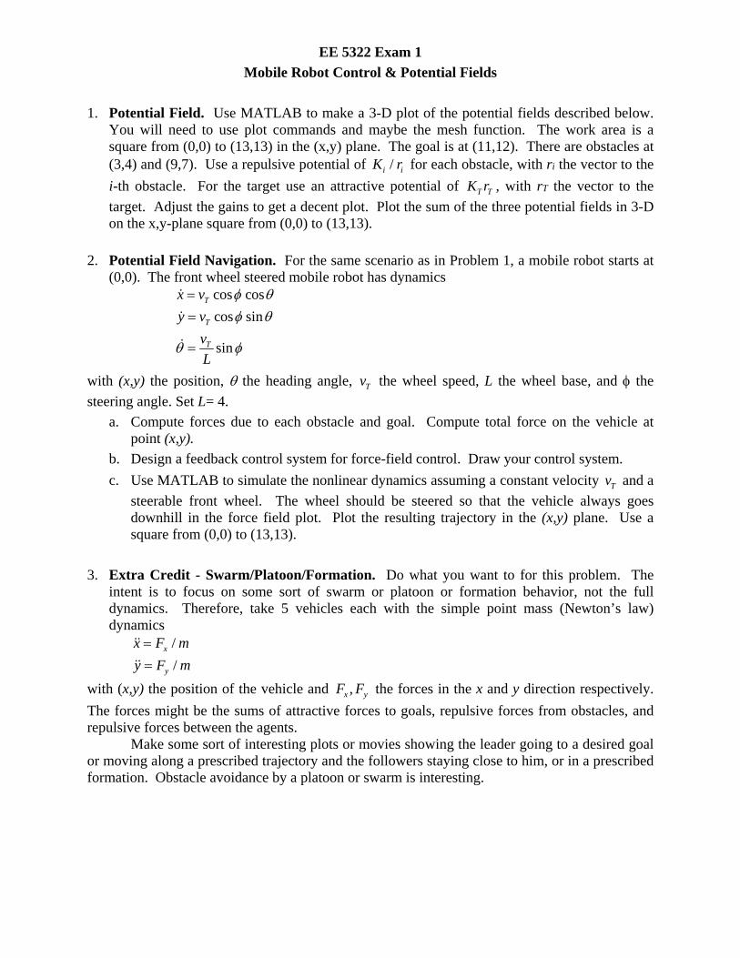
1. Potential Field. Use MATLAB to make a 3-D plot of the potential fields described below. You will need to use plot commands and maybe the mesh function. The work area is a square from (0,0) to (13,13) in the (x,y) plane. The goal is at (11,12). There are obstacles at (3,4) and (9,7). Use a repulsive potential of /i iK r for each obstacle, with ri the vector to the
i-th obstacle. For the target use an attractive potential of T TK r , with rT the vector to the
target. Adjust the gains to get a decent plot. Plot the sum of the three potential fields in 3-D on the x,y-plane square from (0,0) to (13,13).
2. Potential Field Navigation. For the same scenario as in Problem 1, a mobile robot starts at (0,0). The front wheel steered mobile robot has dynamics
cos cos
cos sin
sin
T
T
T
x v
y v
v
L
with (x,y) the position, the heading angle, Tv the wheel speed, L the wheel base, and the
steering angle. Set L= 4.
a. Compute forces due to each obstacle and goal. Compute total force on the vehicle at point (x,y).
b. Design a feedback control system for force-field control. Draw your control system.
c. Use MATLAB to simulate the nonlinear dynamics assuming a constant velocity Tv and a
steerable front wheel. The wheel should be steered so that the vehicle always goes downhill in the force field plot. Plot the resulting trajectory in the (x,y) plane. Use a square from (0,0) to (13,13).
3. Extra Credit - Swarm/Platoon/Formation. Do what you want to for this problem. The intent is to focus on some sort of swarm or platoon or formation behavior, not the full dynamics. Therefore, take 5 vehicles each with the simple point mass (Newton’s law) dynamics
/
/x
y
x F m
y F m
with (x,y) the position of the vehicle and ,x yF F the forces in the x and y direction respectively.
The forces might be the sums of attractive forces to goals, repulsive forces from obstacles, and repulsive forces between the agents.
Make some sort of interesting plots or movies showing the leader going to a desired goal or moving along a prescribed trajectory and the followers staying close to him, or in a prescribed formation. Obstacle avoidance by a platoon or swarm is interesting.
EE 5322 Homework 4
Adaptive Control, Robust Control
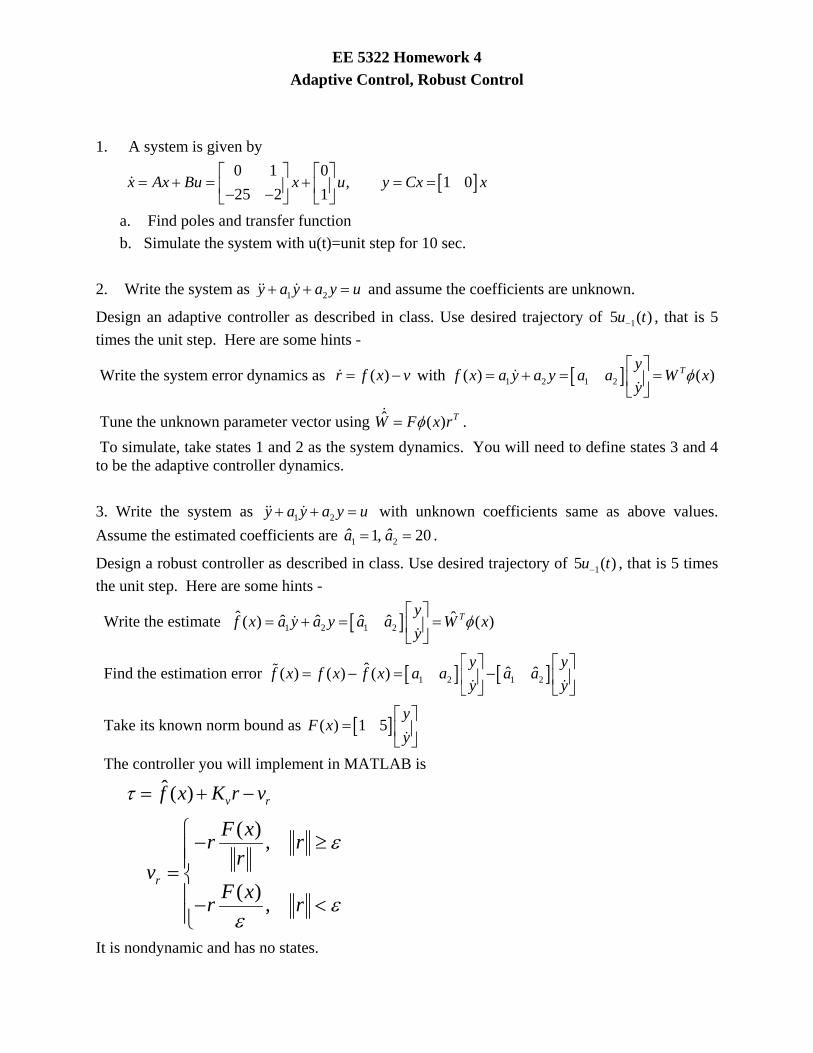
1. A system is given by
0 1 0, 1 0
25 2 1x Ax Bu x u y Cx x
a. Find poles and transfer function
b. Simulate the system with u(t)=unit step for 10 sec.
2. Write the system as 1 2y a y a y u and assume the coefficients are unknown.
Design an adaptive controller as described in class. Use desired trajectory of 15 ( )u t , that is 5
times the unit step. Here are some hints -
Write the system error dynamics as ( )r f x v with 1 2 1 2( ) ( )Tyf x a y a y a a W x
y
Tune the unknown parameter vector using ˆ ( ) TW F x r .
To simulate, take states 1 and 2 as the system dynamics. You will need to define states 3 and 4 to be the adaptive controller dynamics.
3. Write the system as 1 2y a y a y u with unknown coefficients same as above values.
Assume the estimated coefficients are 1 2ˆ ˆ1, 20a a .
Design a robust controller as described in class. Use desired trajectory of 15 ( )u t , that is 5 times
the unit step. Here are some hints -
Write the estimate 1 2 1 2ˆ ˆˆ ˆ ˆ ˆ( ) ( )Tyf x a y a y a a W x
y
Find the estimation error 1 2 1 2ˆ ˆ ˆ( ) ( ) ( )
y yf x f x f x a a a a
y y
Take its known norm bound as ( ) 1 5y
F xy
The controller you will implement in MATLAB is
ˆ ( ) v rf x K r v
( ),
( ),
r
F xr r
rv
F xr r
It is nondynamic and has no states.
EE 5322 Intelligent Control- Exam 2 Fall 2017
1. This is a take home exam. YOU MUST WORK ALONE.
Any cheating or collusion will be severely punished.
2. To obtain full credit, show all your work. No partial credit will be given without the supporting work.
3. Please sign this form and include it as the first page of your submitted exam.
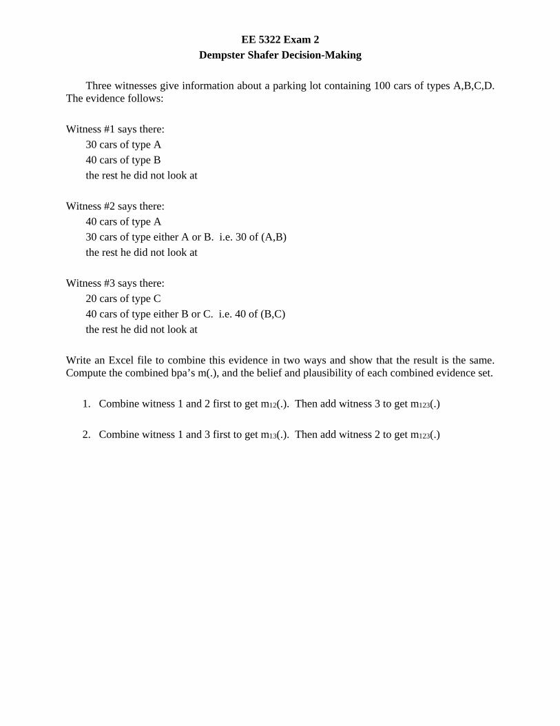
Three witnesses give information about a parking lot containing 100 cars of types A,B,C,D. The evidence follows:
Witness #1 says there:
30 cars of type A
40 cars of type B
the rest he did not look at
Witness #2 says there:
40 cars of type A
30 cars of type either A or B. i.e. 30 of (A,B)
the rest he did not look at
Witness #3 says there:
20 cars of type C
40 cars of type either B or C. i.e. 40 of (B,C)
the rest he did not look at
Write an Excel file to combine this evidence in two ways and show that the result is the same. Compute the combined bpa’s m(.), and the belief and plausibility of each combined evidence set.
1. Combine witness 1 and 2 first to get m12(.). Then add witness 3 to get m123(.)
2. Combine witness 1 and 3 first to get m13(.). Then add witness 2 to get m123(.)
EE 5322 Homework 5
Discrete Time Simulation, Observers, Kalman Filter
1. Discrete-Time System.
A discrete time system is given by
kkk BuAxx 1 , 0x
Write a MATLAB m file to simulate the system, i.e. to compute kx for a given input ku , initial
condition 0x , and range of the time index k= 1,2,…,N.
a. Simulate the system
kkk uxx
1
0
8.189.0
101
for ku equal to the unit step and 0x =0. Plot kx vs. k for 100 time samples.
Find the period and percent overshoot.
b. Simulate the same system but now add process noise so that
kkkk wBuAxx 1 .
Take the noise kw as uniformly distributed between 0 and 0.2. Use MATLAB function rand.
Plot kx vs. k for 100 time samples.
2. DT Kalman Filter
Write a MATLAB m file to simulate a DT system
kkkk GwBuAxx 1
kkk vHxz
plus DT Kalman Filter.
Simulate the optimal time-varying DT Kalman Filter for the system
kkkk wuxx
1
0
8.189.0
101 ,
kkk vxz ]01[ .
Take the process noise kw as a normal 2-vector (MATLAB function randn) with each
component having zero mean and variance 0.1. Take measurement noise kv as normal (0,0.1).
Use ku equal to the unit step and 0x =0.
Plot the states and their estimates on the same graphs. i.e. )(ˆ),( 11 kxkx on one graph, and
)(ˆ),( 22 kxkx on another graph.
3. Steady-state DT Kalman Filter
a. Find the steady-state Kalman gain by iteration on the time-varying Riccati difference equation.
b. Find the steady-state Kalman gain by solution of the ARE using dlqe in MATLAB.
c. Simulate the system in problem 2 with the steady-state Kalman Filter, which has a constant gain. Compare the results with the optimal Kalman filter in problem 2.
DO NOT WORK BEYOND THIS PAGE ASSIGNMENTS BEYOND THIS MAY CHANGE
This exam is out of date EE 5322 Exam 1
DT Observer, DT Kalman Filter
1. DT Observer
Write a MATLAB m file to simulate a DT system plus a DT observer running at the same time, as follows.
a. Design an observer for the system
kkk uxx
1
0
9.19425.0
101 , 0x =0
kk xz ]01[
In eqs (2.6), (2.7) in the book use 1.0, TT DDIGG . Find the observer gain L and write down the observer state equation (2.2). You can use routine dlqe in MATLAB.
b. Simulate the system and the observer together using ku equal to the unit step. Select initial
conditions 0 0ˆ[10 10] , 0Tx x . Plot the states and their estimates on the same graphs. i.e.
)(ˆ),( 11 kxkx on one graph, and )(ˆ),( 22 kxkx on another graph. Use 200 samples.
2. DT Kalman Filter
Write a MATLAB m file to simulate a DT system
kkkk GwBuAxx 1
kkk vHxz
plus DT Kalman Filter.
Simulate the optimal time-varying DT Kalman Filter for the system
1
0 1 0 0
0.9425 1.9 1 0.1k k k kx x u w
,
kkk vxz ]01[ .
Take the process noise kw as normal with covariance Q=0.1. Take measurement noise kv as
normal (0,0.1). Use ku equal to the unit step.
Plot the states and their estimates on the same graphs. i.e. )(ˆ),( 11 kxkx on one graph, and
)(ˆ),( 22 kxkx on another graph. Select initial conditions 0 0ˆ[10 10] , 0Tx x .
3. Steady-state DT Kalman Filter
a. Find the steady-state Kalman gain by iteration on the time-varying Riccati difference equation.
b. Find the steady-state Kalman gain by solution of the ARE using dlqe in MATLAB.
c. Simulate the system in problem 2 with the steady-state Kalman Filter, which has a constant gain. Select initial conditions 0 0ˆ[10 10] , 0Tx x . Compare the results with the optimal
Kalman filter in problem 2.
EE 5322 Homework 4
Mobile Robot Control & Potential Fields
4. Potential Field. Use MATLAB to make a 3-D plot of the potential fields described below. You will need to use plot commands and maybe the mesh function. The work area is a square from (0,0) to (12,12) in the (x,y) plane. The goal is at (10,10). There are obstacles at (3,3) and (9,9). Use a repulsive potential of /i iK r for each obstacle, with ri the vector to the
i-th obstacle. For the target use an attractive potential of T TK r , with rT the vector to the
target. Adjust the gains to get a decent plot. Plot the sum of the three potential fields in 3-D on the x,y-plane square from (0,0) to (12,12).
5. Potential Field Navigation. For the same scenario as in Problem 1, a mobile robot starts at (0,0). The front wheel steered mobile robot has dynamics
cos cos
cos sin
sin
T
T
T
x v
y v
v
L
with (x,y) the position, the heading angle, Tv the wheel speed, L the wheel base, and the
steering angle. Set L= 2.
d. Compute forces due to each obstacle and goal. Compute total force on the vehicle at point (x,y).
e. Design a feedback control system for force-field control. Draw your control system.
f. Use MATLAB to simulate the nonlinear dynamics assuming a constant velocity Tv and a
steerable front wheel. The wheel should be steered so that the vehicle always goes downhill in the force field plot. Plot the resulting trajectory in the (x,y) plane. Use a square from (0,0) to (12,12).
6. Platoon of Mobile Robots.
There are 3 robots in a platoon. Robot 1 is the leader. For each robot i take the simplified Newton’s law dynamics (with mass=1)
i
i x
ii y
x F
y F
with (x,y) the position of the vehicle and ,x yF F the forces in the x and y direction respectively.
The obstacles and goal are the same as in problems 1 and 2.
a. Program the forces for the leader node 1 to avoid the obstacles and go to the target. Same scenario as above (but with these simplified dynamics).
b. Program the force on each follower to stay ½ unit from the leader and not to run into each other. Use repulsive POTENTIAL between followers as 2/i ijK r with rij= distance
between followers i and j. For the potential to the leader, use something like
212 ( )iL iL DV r r
with riL the distance from follower i to the leader, and rD the desired separation. Play with the potentials to make it work properly. Compute forces properly using calculus.
c. Simulate. Plots trajectories in (x,y) plane. Start all robots at (0,0).
EE 5322 Homework 5
Neural Networks
1- Consider the following training data set
a- Train a perceptron to classify the data set into two classes. Plot points and
decision boundaries. b- Use a single neuron with sigmoid activation function to do this classification
problem. Plot the points and decision boundary and compare the results to part a.
2- Consider the dynamical system
30.1 ( )x x f x
where 2( ) 2cos( )f x x x .
a) Approximate the function f(x) using an MLP neural network and plot the function and the estimation on the same graph.
b) Simulate the system response for exact f(x) and the approximation. Use different initial conditions. Compare the results.
EE 5322 Homework 6
Fuzzy Logic
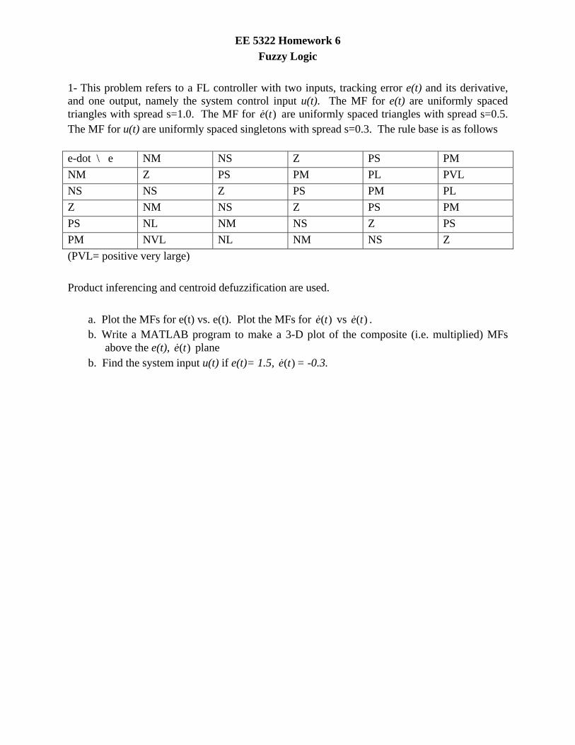
1- This problem refers to a FL controller with two inputs, tracking error e(t) and its derivative, and one output, namely the system control input u(t). The MF for e(t) are uniformly spaced triangles with spread s=1.0. The MF for )(te are uniformly spaced triangles with spread s=0.5. The MF for u(t) are uniformly spaced singletons with spread s=0.3. The rule base is as follows
e-dot \ e NM NS Z PS PM
NM Z PS PM PL PVL
NS NS Z PS PM PL
Z NM NS Z PS PM
PS NL NM NS Z PS
PM NVL NL NM NS Z
(PVL= positive very large)
Product inferencing and centroid defuzzification are used.
a. Plot the MFs for e(t) vs. e(t). Plot the MFs for )(te vs )(te . b. Write a MATLAB program to make a 3-D plot of the composite (i.e. multiplied) MFs
above the e(t), )(te plane b. Find the system input u(t) if e(t)= 1.5, )(te = -0.3.
EE 5322 Intelligent Control- Exam 2 Fall 2015
1. This is a take home exam. YOU MUST WORK ALONE.
Any cheating or collusion will be severely punished.
2. To obtain full credit, show all your work. No partial credit will be given without the supporting work.
3. Please sign this form and include it as the first page of your submitted exam.
Three witnesses give information about a parking lot containing 100 cars of types A,B,C,D. The evidence follows:
Witness #1 says there:
30 cars of type A
40 cars of type C
the rest he did not look at
Witness #2 says there:
40 cars of type A
30 cars of type either A or C. i.e. 30 of (A,C)
the rest he did not look at
Witness #3 says there:
20 cars of type B
40 cars of type either B or C. i.e. 40 of (B,C)
the rest he did not look at
Write an Excel file to combine this evidence in two ways and show that the result is the same. Compute the combined bpa’s m(.), and the belief and plausibility of each combined evidence set.
3. Combine witness 1 and 2 first to get m12(.). Then add witness 3 to get m123(.)
4. Combine witness 1 and 3 first to get m13(.). Then add witness 2 to get m123(.)
DO NOT DO THE FOLLOWING HOMEWORKS YET.
THEY WILL CHANGE
from Rabiner and Schafer, 1978
EE 5322 Homework 2
RLS and DFT Analysis
Download the file for this problem from the homework assignment home page. Do not worry about the file name. It is the correct file for this problem.
1. RLS System Identification
The input ku and output ky of a discrete time system are given in the data file. The system
is of second order with a delay of d=2.
a. Write a RLS program to identify the system transfer function.
b. Plot the output ky and the output of your identified system given the input ku . They should
be the same.
2. Digital Speech Processing
(The frequencies here are about 1/10 the actual values for ease of processing using MATLAB.)
In speech, the vowels are characterized by three main frequencies known as formants. The first two formants for each vowel in English are as follows:
vowel Formant 1 (Hz) Formant 2 (Hz)
A 70 110
E 50 180
I 40 200
O 60 80
U 30 80
The data for this homework contains an 8 sec speech signal that contains some vowels. The sampling period is 1 msec= 0.001 sec. Chop the signal into eight bins of length 1 sec. In each bin, do the FFT (using N= a power of two).
Determine which vowels occur and when. Finally, plot the DFT vs. time as a 3-D plot.
3. Machinery Monitoring
An induction motor drive has a base rotation frequency of 0f = 50 Hz, a frequency of 3 0f
due to a three-bladed fan, and a component at 4 0f due to a 4:1 gearbox. When a certain pinion
gear wears badly enough, a prominent frequency component of 277 Hz appears. Soon after that, the amplitude of the frequency component at 4 0f significantly increases due to the failure of a
gear tooth.
In the 6 sec data file, the sampling period is 1 msec. Find out when the two anomaly failure events occur. Plot the DFT vs. time as a 3-D plot. Use moving average window for the DFT of length ½ sec. Use N= a power of two.
EE 5322 Homework 3
Discrete Time Simulation, Observers, Kalman Filter
1. Discrete-Time System.
A discrete time system is given by
kkk BuAxx 1 , 0x
Write a MATLAB m file to simulate the system, i.e. to compute kx for a given input ku , initial
condition 0x , and range of the time index k= 1,2,…,N.
a. Simulate the system
kkk uxx
1
0
8.189.0
101
for ku equal to the unit step and 0x =0. Plot kx vs. k for 100 time samples.
Find the period and percent overshoot.
b. Simulate the same system but now add process noise so that
kkkk wBuAxx 1 .
Take the noise kw as uniformly distributed between 0 and 0.2. Use MATLAB function rand.
Plot kx vs. k for 100 time samples.
2. DT Kalman Filter
Write a MATLAB m file to simulate a DT system
kkkk GwBuAxx 1
kkk vHxz
plus DT Kalman Filter.
Simulate the optimal time-varying DT Kalman Filter for the system
kkkk wuxx
1
0
8.189.0
101 ,
kkk vxz ]01[ .
Take the process noise kw as a normal 2-vector (MATLAB function randn) with each
component having zero mean and variance 0.1. Take measurement noise kv as normal (0,0.1).
Use ku equal to the unit step and 0x =0.
Plot the states and their estimates on the same graphs. i.e. )(ˆ),( 11 kxkx on one graph, and
)(ˆ),( 22 kxkx on another graph.
3. Steady-state DT Kalman Filter
a. Find the steady-state Kalman gain by iteration on the time-varying Riccati difference equation.
b. Find the steady-state Kalman gain by solution of the ARE using dlqe in MATLAB.
c. Simulate the system in problem 2 with the steady-state Kalman Filter, which has a constant gain. Compare the results with the optimal Kalman filter in problem 2.
EE 5322 Intelligent Control- Exam 1 Spring 2014
1. This is a take home exam. YOU MUST WORK ALONE.
Any cheating or collusion will be severely punished.
2. To obtain full credit, show all your work. No partial credit will be given without the supporting work.
3. The three problems are weighted equally
4. Please sign this form and include it as the first page of your submitted exam.
7. Potential Field. Use MATLAB to make a 3-D plot of the potential fields described below. You will need to use plot commands and maybe the mesh function. The work area is a square from (0,0) to (10,10) in the (x,y) plane. The goal is at (10,10). There are obstacles at (3,2) and (7,6). Use a repulsive potential of /i iK r for each obstacle, with ri the vector to the
i-th obstacle. For the target use an attractive potential of T TK r , with rT the vector to the
target. Adjust the gains to get a decent plot. Plot the sum of the three potential fields in 3-D.
8. Potential Field Navigation. For the same scenario as in Problem 1, a mobile robot starts at (0,0). The front wheel steered mobile robot has dynamics
sin
coscos
sincos
L
V
Vy
Vx
with (x,y) the position, the heading angle, V the wheel speed, L the wheel base, and the steering angle. Set L= 2.
g. Compute forces due to each obstacle and goal. Compute total force on the vehicle at point (x,y).
h. Design a feedback control system for force-field control. Draw your control system.
i. Use MATLAB to simulate the nonlinear dynamics assuming a constant velocity V and a steerable front wheel. The wheel should be steered so that the vehicle always goes downhill in the force field plot. Plot the resulting trajectory in the (x,y) plane. Use a square from (0,0) to (12,12).
9. Platoon of Mobile Robots.
There are 5 robots in a platoon. Robot 1 is the leader. For each robot i take the simplified Newton’s law dynamics (with mass=1)
i
i x
ii y
x F
y F
with (x,y) the position of the vehicle and ,x yF F the forces in the x and y direction respectively.
c. Program the forces for the leader node 1 to avoid the obstacles and go to the target. Same scenario as above (but with these simplified dynamics).
d. Program the force on each follower to stay ½ unit from the leader and not to run into each other. Use repulsive POTENTIAL between followers as 2/i ijK r with rij= distance
between followers i and j. For the potential to the leader, use something like
212 ( )iL iL DV r r
with riL the distance from follower i to the leader, and rD the desired separation. Play with the potentials to make it work properly. Compute forces properly using calculus.
c. Simulate. Plots trajectories in (x,y) plane. Start all robots at (0,0).
4. 20% EXTRA CREDIT- Make a routine to plot the robots as points on the screen in real-time as the robots move. Then, you can see them move.
If you feel like it, make a movie too. Use MATLAB fns moviein, getframe, etc.
EE 5322 Homework 4 (Neural Networks)
3- Consider the following training data set
c- Train a perceptron to classify the data set into two classes. Plot points and
decision boundaries. d- Use a single neuron with sigmoid activation function to do this classification
problem. Plot the points and decision boundary and compare the results to part a.
4- Consider the dynamical system
30.1 ( )x x f x=- +
where 2( ) sin( )f x x x= + .
c) Approximate the function f(x) using an MLP neural network and plot the function and the estimation on the same graph.
d) Simulate the system response for exact f(x) and the approximation. Use different initial conditions. Compare the results.
For the following two questions, download the breast cancer data from your blackboard and load it into your MATLAB session. This file contains a matrix called data of size 683 × 11, which represents 9 measurements (various geometric features) taken from images of 683 cells in breasts. data(j,1) is the Id. number of the jth cell, data(j,2:10) contains those 9 measurements of the jth cell, and data(j,11) contains the diagnosis by the doctors, i.e., benign if this value is 2; malignant if this value is 4.
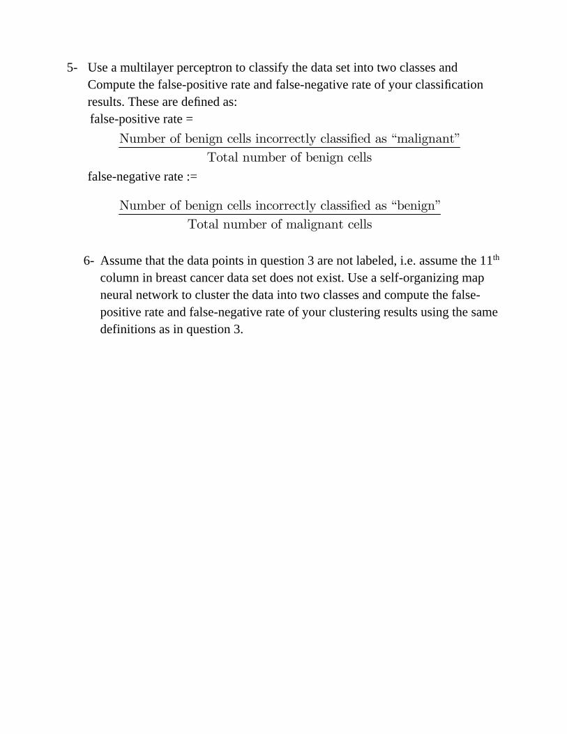
5- Use a multilayer perceptron to classify the data set into two classes and Compute the false-positive rate and false-negative rate of your classification results. These are defined as: false-positive rate =
Number of benign cells incorrectly classi ed as “malignant”
Total number of benign cells
false-negative rate :=
Number of benign cells incorrectly classi ed as “benign”
Total number of malignant cells
6- Assume that the data points in question 3 are not labeled, i.e. assume the 11th
column in breast cancer data set does not exist. Use a self-organizing map neural network to cluster the data into two classes and compute the false-positive rate and false-negative rate of your clustering results using the same definitions as in question 3.
EE 5322 Homework # 5 (Fuzzy Logic)
2- This problem refers to a FL controller with two inputs, tracking error e(t) and its derivative, and one output, namely the system control input u(t). The MF for e(t) are uniformly spaced triangles with spread s=1.2. The MF for )(te are uniformly spaced triangles with spread s=0.4. The MF for u(t) are uniformly spaced singletons with spread s=0.2. The rule base is as follows
e-dot \ e NM NS Z PS PM
NM Z PS PM PL PVL
NS NS Z PS PM PL
Z NM NS Z PS PM
PS NL NM NS Z PS
PM NVL NL NM NS Z
(PVL= positive very large)
Product inferencing and centroid defuzzification are used.
c. Sketch the MFs. d. Write a MATLAB program to make a 3-D plot of the composite (i.e. multiplied) MFs
above the e(t), )(te plane b. Find the system input u(t) if e(t)= 1.5, )(te = -0.3.
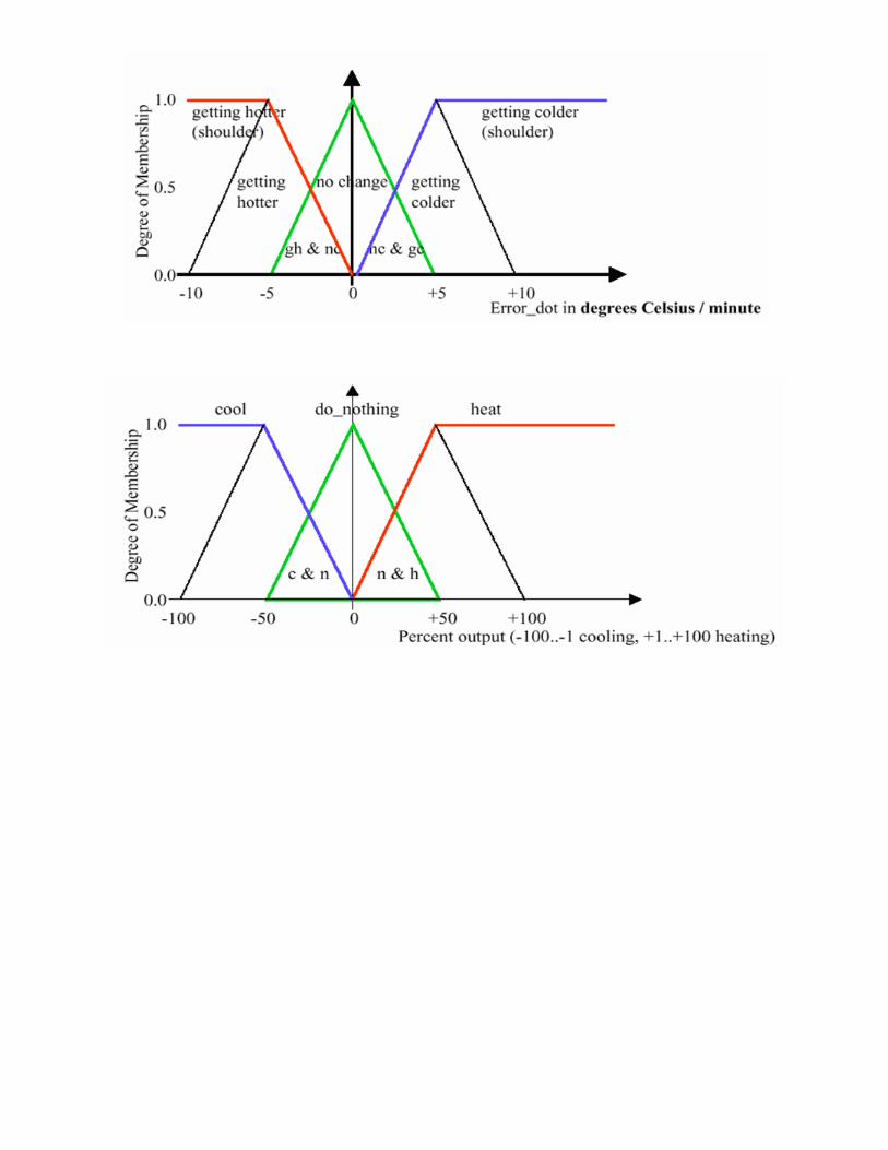
3- Assume that we have two inputs and one output with the following membership functions for control of the temperature. Implement the inputs and output membership functions in MATLAB FIS toolbox and show ~64 % cooling output for error = -1 and error_dot=-2.5. Include MATLAB FIS Rule viewer and print in your report showing the error, error_dot and output.
EE 5322 Intelligent Control- Exam 2 Spring 2014
1. This is a take home exam. YOU MUST WORK ALONE.
Any cheating or collusion will be severely punished.
2. To obtain full credit, show all your work. No partial credit will be given without the supporting work.
3. The three problems are weighted equally
4. Please sign this form and include it as the first page of your submitted exam.
1- Character Recognition using Neural Networks: In this question you are asked to design and train a neural network to recognize the 26 letters of the English alphabet.
You must use the matlab program “prprob” to create the letters and the targets for this character recognition question. That is,
[X,T]=prprob;
where the input X is a 35×26 matrix and target T is a binary 26×26 matrix. In fact, the data consists of the 26 characters of the alphabet and each letter is actually a 7×5 grid of numbers, where 1 is black and 0 is white. Also, each target vector in T is a 26-element vector with a ‘1’ in the position of the letter it represents, and 0’s everywhere else. For example, the letter A is to be represented by a 1 in the first element (as A is the first letter of the alphabet), and 0’s in elements two through twenty-six.
To view a certain character, use the built-in program plotchar. To see the letter A for example, type
plotchar(X(:,1))
A- Build a neural network with one hidden layer and train it using the data provided by prprob (data without noise). Show that the network successfully classifies the characters.
B- In practical situations, the imaging system is not perfect and the letters may suffer from noise. In order to test your network, produce noisy samples by adding noise to the first 5 characters. Apply these samples to the network. Print the network output and plot the character (using plotchar) for these test samples. How accurate your network is in prediction of noisy characters?
Note: Use matlab command letter(:,i)+=X(:,i)+noiseLevel*randn(35,1) (i=1:5) to add noise to the first 5 characters. Try different values of noiseLevel (0.1, 0.2, 0.4 and 0.5) and compare the results.
C- Instead of using only data without noise for training the network, produce 3 noisy samples for each character and use all 104 samples (with and without noise) to train the network. Now apply the test data you built in part B to test the network. Compare the performance to par B.
DO NOT DO THE FOLLOWING HOMEWORKS YET.
THEY WILL CHANGE
EE 5322 Homework 5
Dempster Shafer Decision-Making
Three witnesses give information about a parking lot containing 100 cars of types A,B,C,D. The evidence follows:
Witness #1 says there:
20 cars of type A
30 cars of type C
the rest he did not look at
Witness #2 says there:
20 cars of type A
30 cars of type either A or C. i.e. 30 of (A,C)
the rest he did not look at
Witness #3 says there:
20 cars of type B
20 cars of type either B or C. i.e. 20 of (B,C)
the rest he did not look at
Write an Excel file to combine this evidence in two ways and show that the result is the same. Compute the combined bpa’s m(.), and the belief and plausibility of each combined evidence set.
5. Combine witness 1 and 2 first to get m12(.). Then add witness 3 to get m123(.)
6. Combine witness 1 and 3 first to get m13(.). Then add witness 2 to get m123(.)
EE 5322 Homework 6
Fuzzy Logic
1. This problem refers to a FL controller with two inputs, tracking error e(t) and its derivative, and one output, namely the system control input u(t). The MF for e(t) are uniformly spaced triangles with spread (i.e. base width) s=0.5. The MF for )(te are uniformly spaced triangles with spread s=1.0. The MF for u(t) are uniformly spaced singletons with spread s=0.5. The rulebase is as follows
e-dot \ e NM NS Z PS PM
NM Z PS PM PL PVL
NS NS Z PS PM PL
Z NM NS Z PS PM
PS NL NM NS Z PS
PM NVL NL NM NS Z
(PVL= positive very large)
Product inferencing and centroid defuzzification are used.
a. Sketch the MFs.
b. Write a MATLAB program to make a 3-D plot of the composite (i.e. multiplied) MFs above the e(t), )(te plane
b. Find the system input u(t) if e(t)= 0.4, )(te = -0.8.
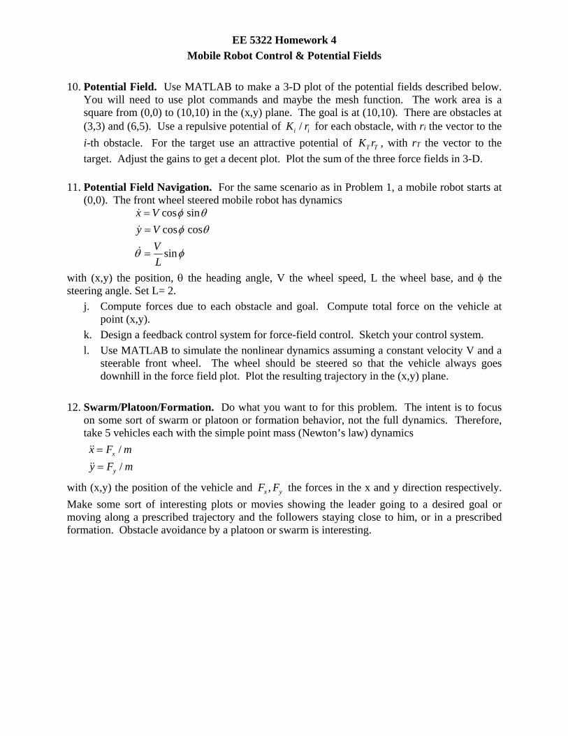
EE 5322 Homework 4
Mobile Robot Control & Potential Fields
10. Potential Field. Use MATLAB to make a 3-D plot of the potential fields described below. You will need to use plot commands and maybe the mesh function. The work area is a square from (0,0) to (10,10) in the (x,y) plane. The goal is at (10,10). There are obstacles at (3,3) and (6,5). Use a repulsive potential of /i iK r for each obstacle, with ri the vector to the
i-th obstacle. For the target use an attractive potential of T TK r , with rT the vector to the
target. Adjust the gains to get a decent plot. Plot the sum of the three force fields in 3-D.
11. Potential Field Navigation. For the same scenario as in Problem 1, a mobile robot starts at (0,0). The front wheel steered mobile robot has dynamics
sin
coscos
sincos
L
V
Vy
Vx
with (x,y) the position, the heading angle, V the wheel speed, L the wheel base, and the steering angle. Set L= 2.
j. Compute forces due to each obstacle and goal. Compute total force on the vehicle at point (x,y).
k. Design a feedback control system for force-field control. Sketch your control system.
l. Use MATLAB to simulate the nonlinear dynamics assuming a constant velocity V and a steerable front wheel. The wheel should be steered so that the vehicle always goes downhill in the force field plot. Plot the resulting trajectory in the (x,y) plane.
12. Swarm/Platoon/Formation. Do what you want to for this problem. The intent is to focus on some sort of swarm or platoon or formation behavior, not the full dynamics. Therefore, take 5 vehicles each with the simple point mass (Newton’s law) dynamics
/
/x
y
x F m
y F m
with (x,y) the position of the vehicle and ,x yF F the forces in the x and y direction respectively.
Make some sort of interesting plots or movies showing the leader going to a desired goal or moving along a prescribed trajectory and the followers staying close to him, or in a prescribed formation. Obstacle avoidance by a platoon or swarm is interesting.
EE 5322 Homework 1
Stock Market Time Series Analysis and DFT
The closing price for the NASDAQ tracking stock NVDA is given as an Excel file.
Note there are 254 trading days in the year. There are about 22 trading days in a month. Therefore, for trading on a monthly time scale, one considers a 20-day time window. This allows one to capture many motions of the stock while not spending too much in broker’s fees by churning the stock. On-line trades now run about $15 per transaction.
1. a. Compute the 20 day MA. Plot on the same figure as the stock closing price.
b. Plot the stock minus the 20 day MA.
c. Compute and plot the 20 day moving sample variance.
d. On the same figure, plot the stock closing price, the 20 day MA, and
the MA plus three times the 20 day standard deviation
the MA minus three times the 20 day standard deviation.
The last two lines are known as the Bollinger Bands, after John Bollinger.
2. a. Compute and plot the 20 day moving skew.
b. Compute and plot the 20 day moving kurtosis.
c. Can you use these statistics to find a leading indicator for movements in the stock?
i.e. how can we predict using statistics when the stock is about to break its trend (change its pattern)?
3. a. Compute and plot the autocorrelation.
b. Compute and plot the autocovariance.
4. a. Compute and plot the DFT of the entire signal.
b. Compute and plot the DFT of the entire signal minus the 20 day MA.
c. Compute and plot the time-varying DFT using a moving window of 20 days.
d. Compute and plot the time-varying DFT using fixed bins of 20 days in length.
Any news about predicting movements in this stock?