Do real interest rates converge? Evidence from the European Union by Michael G. Arghyrou* Cardiff Business School Andros Gregoriou Brunel Business School Alexandros Kontonikas University of Glasgow, Department of Economics Abstract We test for real interest parity (RIP) in the EU25 area. Our contribution is two-fold: First, we account for the previously overlooked effects of structural breaks on real interest rate differentials. Second, we test for RIP against the EMU average. For the majority of our sample countries we obtain evidence of real interest rate convergence towards the latter. Convergence, however, is a gradual process subject to structural breaks, typically falling close to the launch of the euro. Our findings have important implications relating to the single monetary policy and the progress new EU members have achieved towards joining the euro. Keywords: real interest rate parity; convergence, structural breaks; EU; EMU; JEL classification: F21, F32, C15, C22 * Corresponding author; Michael G Arghyrou, Cardiff Business School, Cardiff, CF10 3EU, UK. Tel. No. ++44(0)2920875515; Fax No. ++44(0)2920874419; E-mail: [email protected]
Transcript
Do real interest rates converge?
Evidence from the European Union
by
Michael G. Arghyrou*
Cardiff Business School
Andros Gregoriou
Brunel Business School
Alexandros Kontonikas
University of Glasgow, Department of Economics
Abstract
We test for real interest parity (RIP) in the EU25 area. Our contribution is two-fold:
First, we account for the previously overlooked effects of structural breaks on real
interest rate differentials. Second, we test for RIP against the EMU average. For the
majority of our sample countries we obtain evidence of real interest rate convergence
towards the latter. Convergence, however, is a gradual process subject to structural
breaks, typically falling close to the launch of the euro. Our findings have important
implications relating to the single monetary policy and the progress new EU members
have achieved towards joining the euro.
Keywords: real interest rate parity; convergence, structural breaks; EU; EMU;
JEL classification: F21, F32, C15, C22
* Corresponding author; Michael G Arghyrou, Cardiff Business School, Cardiff, CF10
Uncovered Interest Parity (UIP) and Purchasing Power Parity (PPP), two
cornerstone parity conditions in international macroeconomics, imply, when combined,
that expected real returns are equalised across countries. This proposition, known as
Real Interest Parity (RIP), has significant implications for international investors and
policy-makers alike: If national real interest rates were bound to converge, the scope for
international portfolio diversification would be significantly reduced; and national
monetary policy as a tool of effective macro-management would be restricted to the
degree it affects the international real interest rate (see Mark, 1985).1
Due to its important consequences, RIP has attracted considerable empirical
attention. The existing literature has mainly focused on RIP against the USA evolving
significantly over time. Early studies, such as Mishkin (1984a, 1984b), Cumby and
Obstfeld (1984) and Mark (1985) tested, and generally rejected, RIP by imposing unity
restrictions on the intercept and slope coefficients in regressions of domestic on foreign
real interest rates. These, however, were criticised for overlooking possible unit roots in
the regression’s variables. A number of authors subsequently tested for cointegration
between the two rates, typically finding mean reversion for the residuals of the
cointegrating regression.2 Nevertheless, this approach was also criticised for allowing
the coefficient of the foreign real interest rate to deviate from its theory-consistent unity
value. Hence, the literature moved towards RIP tests based on real interest rate
differentials (RIRDs) where unity coefficients are by definition imposed.3
1 As RIP underpins a number of mainstream monetary models of exchange determination (see e.g.
Frenkel 1976, Frankel 1979, Mussa 1982) its validity is also important for our understanding of exchange
rate movements and the authorities’ ability to manage them. 2 See Evans et al (1994), Goodwin and Grennes (1994), Chinn and Frankel (1995), Frankel and Okongwu
(1995), Jorion (1996), Moosa and Bhatti (1996), Alexakis et al (1997), Awad and Goodwin (1998).
Phylaktis (1999) and Fujii and Chinn (2000). 3 Alternative tests of RIP include MacDonald and Taylor (1989) and Fraser and Taylor (1990), who test
and reject the RIP-consistent hypothesis according to which nominal interest rate differentials predict
future inflation differentials. Marston (1995) finds that movements of RIRDs can be explained using
2
Early studies adopting this approach (see e.g. Meese and Rogoff, 1988 and
Edison and Pauls, 1993) found unit roots in RIRDs, thus rejecting RIP. These studies,
however, were based on the standard Augmented Dickey Fuller (1979, ADF) test,
known to be subject to a number of drawbacks, including low power and biases in the
presence of structural breaks and non-linearities. Wu and Chen (1998), Gagnon and
Unferth (1995) and Ong et al (1999) increase power through panel data tests, providing
evidence in favour of RIP.4 More recently, a number of studies, including Obstfeld and
Taylor (2002), Nakagawa (2002), Mancuso et al (2003), Holmes and Maghrebi (2006)
and Ferreira and Leon-Ledesma (2007), estimate non-linear models upholding RIRD
mean-reversion, though not always around a zero value.5
Overall, the recent literature has achieved significant progress towards
overturning the early unit root RIRD findings. Yet, some important points remain
unaddressed. Most prominently, the literature has overlooked the potential effects of
structural breaks in RIRD series.6 Such breaks reduce further the already low power of
ADF tests (see Perron, 1989) and may result in non-linear models being erroneously
selected as the best description of an otherwise linear data generation process (see Koop
and Potter, 2001). In recent years, a number of events that may have caused structural
breaks in RIRD series have taken place. These include the introduction of market and
monetary policy reforms in a number of countries and the launch of the European
variables included in the current information set, leading to rejection of the RIP hypothesis. Kugler and
Neusser (1993) adopt a stationary multivariate time-series framework using ex-post real interest rates,
obtaining findings favourable towards RIP. A similar conclusion is reached by Cavaglia (1992) who
applies Kalman filtering techniques to estimate the persistence of ex-ante real interest rate differentials. 4 Obstfeld and Taylor (2002) increase power by using larger sample periods and a generalised least square
version of the ADF test. 5 Non-linear adjustment to RIP is theoretically justified by market imperfections such as those in Dumas
(1992). These include transaction and other sunk costs in international trading, legal obligations imposing
on agents to hold assets for minimum time periods and trading rules postulating that differences between
returns exceed certain thresholds before arbitrage trading is initiated. Such imperfections imply that small
non-zero RIRD values are not arbitraged, while large deviations from zero trigger trading restoring RIP. 6 Fountas and Wu (2000) are an important exception. However, their analysis is undertaken within a
cointegration framework and, as a result, is subject to the critique discussed above.
3
Economic and Monetary Union (EMU) in Europe in 1999. Lack of investigation of the
effects of such events is surprising, particularly given that the appropriate econometric
methods are now well-developed. The first contribution of this paper is to precisely fill
this gap, i.e. to analyse international real interest rate convergence accounting for
structural breaks in the RIRD series.
We focus on the European Union (EU), an area whose members (old and new)
have all experienced one or more of the potential breaks mentioned above. Previous
studies on Europe test RIP against Germany (see e.g. Holmes 2002 and 2005, Leon-
Ledesma 2007). We instead test, for the first time to the best of our knowledge, RIP
against the EMU average. This is the second contribution of this paper, as our analysis
provides important insights relating to the workings of the single currency. The reason
is the following: The European Central Bank (ECB) operates under an institutional
mandate to set nominal interest rates for the EMU average. The ECB 2 per cent inflation
objective also refers to the EMU average. In practise, therefore, the ECB is meant to
conduct monetary policy in the interests of the Euroland as a whole by way of
managing the EMU average real interest rate (see Aksoy et al, 2002).7 Changes in the
latter are exactly the channel through which the single monetary policy is meant to be
transmitted to the eurozone’s individual economies. For transmission to be uniform,
national RIRDs against the EMU average must be mean-reverting and display similar
persistence patterns. If the opposite is true, shifts in the eurozone average-oriented ECB
policy would result in intra-EMU asymmetric monetary shocks, posing member-states
with differential, and potentially unwelcome, output gap and asset prices’ responses. All
in all, the degree of convergence of national real interest rates towards the EMU average
7Aksoy et al (2002) argue that this institutionally-mandated “euro-wide” conduct of the single monetary
policy would be welfare maximizing. There is no hard evidence to suggest that this policy is not
implemented in practise, although in a recent paper Heinemann and Huefner (2004) argue that it is
possible that small EMU countries have an excessive, relative to their size, weight in the ECB decision
making process.
4
conveys important information relating to the “one size fits all” monetary policy debate.
Furthermore, by assuming both UIP and PPP, RIP is a comprehensive measure of
economic integration among countries that are candidates to form a common currency
area. As textbook monetary union theory suggests, the net cost of abolishing national
currencies is a negative function of the degree of integration between the prospective
union’s member states. Hence, the degree of real interest rate convergence between the
new EU members and the EMU average provides useful insights relating to the progress
the former have achieved towards adopting the euro.
Our econometric analysis is comprehensive as it covers all but one EU25
countries.8 Following the majority of existing studies, it is based on ex-post real interest
rates calculated using identical definitions for nominal interest and inflation rates (see
section 2 below). This eliminates biases due to invalid approximations of inflation
expectations (see e.g. Ferreira and Leon-Ledesma, 2007) and/or non-identical
definitions of real returns (see e.g. Dutton, 1993). Data availability defines our sample
to cover 1996-2005 (monthly frequency), a decade characterised by full capital mobility
within Europe, free, in relation to the new EU countries, from the original shock of
transition of the early 1990s. We extend the standard ADF unit root tests first by
correcting for residuals’ heterescedasticity and normality applying the wild-bootstrap
simulation technique used by Arghyrou and Gregoriou (2007); then by accounting for
the effects of structural breaks on RIRD series. These turn out to be captured by the
minimum Lagrange Multiplier (LM) unit root test by Lee and Strazicich (2003), which
allows for two endogenous structural breaks in the series’ level and/or trend and has
superior econometric properties against alternative endogenous single-breaks tests, such
as the one by Perron (1997).
8 Due to data limitations, we had to exclude Luxembourg from our analysis.
5
Our findings turn out to be novel and interesting: First, we reject the null of unit
root RIRD behaviour for 21 out of 24 sample countries. Allowing for two rather than
one or no structural breaks is critical in this respect. Second, structural breaks fall close
to important economic events, most prominently (but not exclusively) the euro’s launch
in 1999. Third, we find evidence of rapid real interest rate convergence in the EMU area
prior to 1999 followed by divergence between some “core” and “periphery” EMU
countries (as well as the UK) thereafter. Fourth, we find that most (though not all) of the
new EU members have achieved convergence to the EMU average by the end of 2005.
Overall, our findings are generally favourable towards RIP in the EU area.
Convergence, however, is found to be a gradual process subject to structural breaks. In
addition, there exist some important country-specific exceptions for which convergence
is rejected.
The remainder of the paper is structured as follows: Section 2 outlines our
findings. Finally, section 5 summarises and offers concluding remarks.
2. DATA
Real interest rate differentials can be calculated using either ex-ante or ex-post
real returns, as well as alternative definitions for nominal interest and inflation rates.
Following the majority of existing studies we use ex-post real returns so as to bypass the
empirically tricky subject of approximating empirically inflation expectations. Also, to
minimize the influence of factors such as foreign-exchange risk, whose role is more
prominent in interest rates of longer-maturity (see e.g. Ferreira and Leon-Ledesma,
2007)., we define nominal interest rates as the three-month money market rate. Finally,
to eliminate biases relating to different definitions of national price levels (see e.g.
6
Dutton, 1993), inflation rates are calculated for all countries using the harmonised
consumer price index (HCPI).
HCPI data is available for the post-1996 period only. This defines our sample to
cover 1996-2005 (a total of 120 monthly observations),9 a period when the vast majority
of capital controls had been abolished in the EU area. Data for three-month money
market rates and HCPI series is taken from the Eurostat Databank provided by
Datastream. The monthly HCPI series exhibit strong seasonality patterns for which we
account by seasonal adjustment.10 As we consider investments of three-month maturity,
we transform the quoted annualised three-month nominal interest rates into a three-
month continuously compounded nominal rate of return. Then, following Ferreira and
Leon-Ledesma (2007), for every period t we calculate ex-post real interest rates (rt) as
the difference between the three-month continuously compounded nominal rate of
return observed in period t-3 (it-3,t) minus the percentage change of the HCPI recorded
between period t-3 and t (πt-3,t) Our analysis, therefore, is based on real rates of return
on investments lasting for three months, calculated by rt = (it-3,t) - (πt-3,t). These rates are
then used to construct the RIRD series against the EMU average denoted by (r – r*)t.
The latter, r*t, is calculated using the EMU three-month money market rate and HCPI
series provided by Datastream. Hence, r*t is a weighted average of national real returns
with the weights determined by the source of our data, Eurostat.
Table 1 presents the series’ summary statistics. Three features stand out. First,
RIRDs in the pre-2004 EU countries (EU15), and in particular in the current EMU ones,
are on average smaller and less volatile than those of the new EU members (i.e. the ten
countries that joined the EU in 2004). Furthermore, real interest rates in the former
9 For the old EU members our sample period is three months longer, extending to 1996.03 10 We adjust the series using the Census X11 multiplicative seasonal adjustment method, used by the US
Bureau of Census to seasonally adjust publicly released data. The X11 routine is available in EViews.
7
group are on average more highly correlated with the EMU average. Second, there exist
important differences among individual countries within the same group. For example,
average RIRD in the core EMU countries are in absolute value lower than in the EMU
periphery.11 Similar differences are also observed within the opt-out EU countries
(Denmark, Sweden and the UK) and the new EU members. Finally, for the majority of
our sample countries the estimated RIRD series and are not normally distributed, a
strong indication for the existence of structural breaks.
3. EMPIRICAL METHODOLOGY
The benchmark test of RIP has been widely discussed in the literature (see e.g.
Ferreira and Leon-Ledesma, 2007) so to preserve space we do not present its derivation
here. We restrict ourselves in saying that this is based on the stochastic model given by
equation (1) below:
(r – r*)t = α + ρ (r – r*)t-1 + ut (1)
where ut is a white noise error. Equation (1) can be reformulated as an autoregressive
model of order k given by equation (2)
∆(r – r*)t = α + φ (r – r*)t-1 + 1
( *)k
i t i
i
r rβ −=
∆ −∑ + ut (2)
where φ = 1
1k
i
i
ρ=
−∑ and 1
k
i
i
ρ=∑ = ρ. Equation (2) is an Augmented Dickey-Fuller (ADF)
regression where φ >0 (corresponding in equation (1) to ρ > 1) describes an explosive
process; φ = 0 (ρ =1) random walk behaviour; φ <0 and α≠ 0 (ρ < 1 and α ≠ 0),
stationarity around a non-zero mean; and φ <0 and α = 0 (ρ < 1 and α = 0) stationarity
11Throughout this paper we define core EMU countries to be those EMU members empirical literature
had identified as belonging to a European optimum currency area prior to the introduction of the euro (see
e.g. Bayoumi and Eichengreen 1993). These include France, Germany, Austria and the Benelux countries.
8
around a zero mean. Out of these conditions only the last one is consistent with RIPR.
Equations (1) and (2) can also include a trend term to test for trend- rather than level-
stationarity. In the steady-state, trend stationarity is not consistent with RIP. However,
within a finite sample, a significant trend term might imply (though not necessarily)
deterministic convergence towards RIP (see section 4 below).
The standard ADF test is known to be subject to a number of drawbacks
potentially leading to biased inference. These include deviations from the assumption of
iid distribution for the residual term ut in equation (2), as well as structural breaks in the
series tested for stationarity.12 Regarding the former, given the evidence presented in
Table 1, it is reasonable to expect that the error terms of our preferred ADF
specifications may be non-normal. We address this problem following Arghyrou and
Gregoriou (2007), who correct the critical values of the standard ADF test for
heteroscedasticity and non-normality using the wild bootstrap simulation technique
described in the Appendix. As far as structural breaks are concerned, Perron’s (1989)
initial approach to account for them was to allow for a single exogenously imposed
structural break under both the null and alternative hypotheses. Subsequent literature
has emphasized the need to determine the break endogenously from the data (see e.g.
Zivot and Andrews, 1992; Perron, 1997).13 More recently, the endogenous two-break
minimum LM unit-root test of Lee and Strazicich (LS, 2003) counterbalances the
potential loss of power of tests that ignore more than one break. The test includes breaks
under both the null and the alternative hypotheses, with rejections of the null
12 In addition, the standard ADF test does not capture non-linear mean reversion although, it should be
kept in mind, rather than genuine the latter may be a reflection of either a small number of outliers (see
van Dijk et al, 1999), or structural breaks in the series tested for stationarity (see Koop and Potter, 2001).
We would have liked to investigate the existence of non-linearities in RIRD series over the three sub-
samples identified by our analysis below, however we could not do so due to the resulting small number
of observations in each of the three sub-samples. 13 As these tests have been extensively used in the literature, we do not discuss them here.
9
unambiguously implying stationarity.14 Focusing on RIRD series, a brief description of
the test by LS has as follows: Consider the data generating process described by
*
1( ) , t t t t t tr r Zδ η η λη ϑ−′− = + = + (3)
where Zt is a vector of exogenous variables and tϑ ~ iid N (0, 2
ϑσ ). LS analyze two
alternative models: First, Model A that allows for two shifts in the level of real interest
rate differentials: '
1 2[1, , , ]t t tZ t D D= , where Djt = 1 for t ≥ Tbj + 1 (j=1,2) and 0 otherwise.
Tb indicates the time period when a break occurs. Second, Model C that allows for two
shifts in the series’ level and trend: '
1 2 1 2[1, , , , , ]t t t t tZ t D D DT DT= , where DTjt = t- Tbj for
t ≥ Tbj + 1 (j=1,2) and 0 otherwise. In Model A, the null and alternative hypotheses are
given by equations (4) and (5), respectively:
* *
0 1 1 2 2 1 1( ) ( )t t t t tr r d B d B r rµ υ−− = + + + − + (4)
*
1 1 1 2 2 2( )t t t tr r t d D d Dµ γ υ− = + + + + (5)
where the error terms ( 1 2,t tυ υ ) are stationary processes; Bjt = 1 for t = Tbj + 1 (j=1,2)
and 0 otherwise. For Model C, we add the previously defined Djt terms to (4) and DTjt
terms to (5), respectively. An LM score principle is used to estimate the LS unit root
test statistic based on the following regression model:
*
1
1
( )k
t t t i t i t
i
r r Z S Sδ φ γ ω− −=
′∆ − = ∆ + + ∆ +∑% % (6)
where *( )t t x tS r r Zψ δ= − − −% %% ; t = 2,…,T; δ~ are coefficients in the regression of
*( )tr r∆ − on ∆Zt; *
1 1( )x r r Zψ δ= − − %% , where *
1( )r r− and Z1 denote the first
observations of *( )tr r− and Zt, respectively; and itS −∆~
terms (i = 1,…,k) are included
14 The null hypothesis in the endogenous two-break unit root test of Lumsdaine and Papell (1997)
assumes no structural breaks, while the alternative does not necessarily imply broken trend stationarity.
Thus, rejecting the null may be interpreted as rejection of a unit root with no structural break, and not
necessarily as rejection of a unit root per se.
10
to account for serial correlation. We can consequently test the unit root null hypothesis
by examining the t-statistic (τ~ ) associated with 0=φ .
Following LS we determine the lag length of the itS −∆~
terms using a general to
specific approach.15 More specifically, at each combination of break points λ = (λ1, λ2 )΄
in the time interval [0.1T, 0.9T]16 we start from a maximum of k = 12 (due to monthly
frequency) terms and reduce the model according to whether the last term is significant
at the 10% level. If not, the last term is dropped and the model is re-estimated with k =
11 terms. The process is repeated until a non-zero maximum augmented term is found;
or k is set to zero. The minimum LM unit root test determines the time location of the
two endogenous breaks, λj = Tbj / T, j = 1, 2, using a grid search as follows:
LMτ = )(~Inf λτλ (7)
The break points are located where the test statistic is minimized.17 Compared to
the structural breaks tests by Zivot and Andrews (1992) and Perron (1997) the minimum
LM unit root test shares the endogenous identification of breaks. However, as LS (2003)
demonstrate, it has comparable or higher power, allows for two rather one structural
breaks, and is not subject to spurious rejections of the null when the series is unit root
with breaks. Hence, the minimum LM test has the significant advantage that rejection of
the null unambiguously implies convergence.18
15 As Strazicich et al (2004, p. 135) argue, this approach has been shown to perform well when compared
to alternative data-dependent methods to select the number of the lagged augmented terms (see e.g. Ng
and Perron, 1995). 16 Following LS (2003) we exclude the first and last quintile of the data from this interval so as to ensure
that breaks are not located at the series’ end-points. 17 LS (2003) also propose an alternative minimum LM unit root test, LMρ , determining the time location
of the two breaks using a grid search given by LMρ = )(~Inf λρλ . As results between the two test’s
variants turned out to be very similar, we only discuss those obtained from the LMτ statistic. 18 A drawback of the minimum LM unit root test is that it does not allow for more than two structural
breaks. However, tests of this kind, not subject to the critique of spurious rejection of the null, are not yet
available to empirical researchers. Bai and Perron (2003) have developed a popular test capturing
11
4. EMPIRICAL FINDINGS
4.1. Stationarity analysis
We first test for real interest rate convergence towards the EMU average using
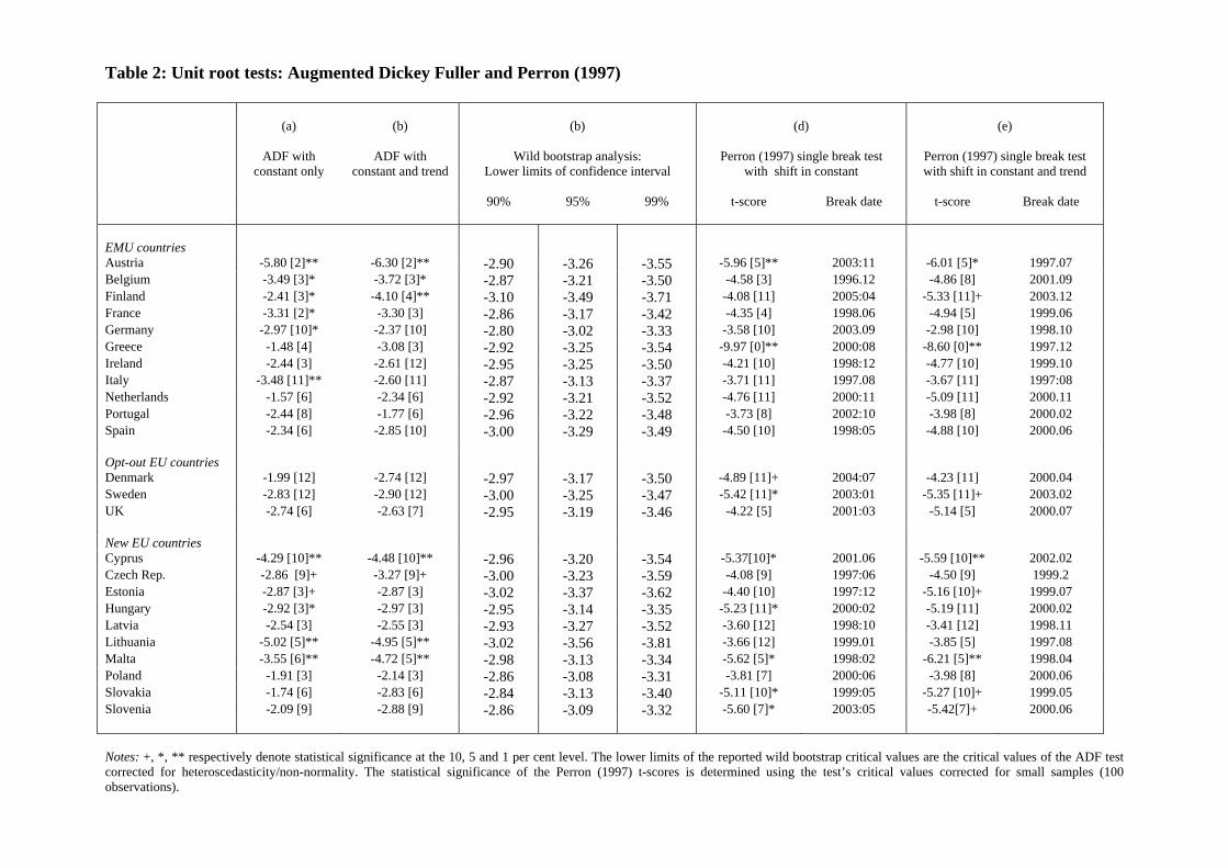
the standard ADF test described by equation (2). The results are reported in Table 2,
column (a). At the 5 per cent level or lower we reject the null of unit root only in 10 out
24 countries. Allowing for a trend term does not increase evidence of stationarity (see
Table 2, column (b)). However, the misspecification tests estimated for the residuals of
our preferred ADF models revealed non-normality and time-varying heteroscedasticity
for the majority of our sample countries.19 We correct for heteroscedasticity and non-
normality using the wild-bootstrap correction applied by Arghyrou and Gregoriou
(2007). This yields the confidence intervals reported in Table 2, column (c).20 The lower
limits of these intervals provide the corrected critical values for the ADF test.21 Our unit
root findings remain robust to this wild bootstrap correction. Indeed, for a number of
countries the latter overturns the previous findings of stationarity.
We now test for stationarity using Perron’s (1997) unit root test allowing for one
endogenous structural break. The results appear in Table 2, columns (d) and (e),
respectively reporting the test’s results allowing for a break in the series’ level; and
level and trend. Compared to the ADF tests, evidence of stationarity does not increase,
as at the 5 per cent level the null of unit root is rejected only in 8 and 4 cases
respectively. Furthermore, as RIRDs have been calculated against the EMU average, the
multiple structural series in linear models. However, their test accounts only for shifts in a series’ mean
(rather than mean and trend) and does not test the null of unit root behaviour. As a result, it is not
applicable in this context of our analysis. As far as the latter is concerned, our tests reported below show
that two breaks are enough to reject the null of unit root in the overwhelming majority of the examined
cases. 19 To preserve space, these are not reported here but are available upon request.
20 Following Arghyrou and Gregoriou (2007) we report the confidence intervals rather then the p-values,
to allow for a more powerful test in the presence of extreme outliers in the data. 21 We have repeated the same analysis for the ADF test with constant and trend. The results, not reported
here but available upon request, remain unaffected.
12
lack of stationarity for almost all EMU countries, including France and Germany,
reduces significantly the plausibility of the reported results.
Finally, we implement the LM minimum unit root test by LS (2003). Our
findings are presented in columns (f) and (g) of Table 2, respectively testing for
stationarity with two breaks in the series’ level; and level and trend. Compared to the
previous results, these make impressive reading, as between them they reject the null of
unit root in 21 out of 24 countries. In these cases, selection between the two alternative
model specifications (indicated with bold letters) is made on the basis of the strongest
rejection of the null.22 Using this criterion, for all but two EU15 countries we select
stationarity with two breaks in the series’ level and trend. For Spain, we select
stationarity with two breaks in the series’ level, whereas Italy is the only EU15 country
where the null is maintained. For the new EU members, the model with two breaks in
level is selected for Latvia, Lithuania, Malta, Slovakia and Slovenia; while the model
with breaks in level and trend is selected for Cyprus, the Czech Republic and Estonia.
Finally, for Hungary and Poland we maintain the null of unit root.
4.2. Structural breaks
The results of the LM-two break unit root test provide interesting insights
relating to the timing of the identified structural breaks. More specifically, our preferred
specifications suggest a break in 1999, the year of EMU’s inception, in six EMU
countries (Belgium, Finland, France, Germany, Ireland, and the Netherlands). For
Greece we obtain a break in 2000.09, three months after the announcement of this
country’s accession to the EMU. Finally, Austria, Portugal and Spain have all
experienced breaks in 2000, the year following the launch of the euro. A break in 2000
may also have taken place in Italy, the only EMU country for which the LMτ test
22 As a robustness test, we repeated the selection exercise using the Akaike information criterion. The
preferred specifications remain identical to those indicated in Table 2 with bold letters.
13
maintains the null of unit root, whereas in Spain, another break had occurred in 1998,
shortly after the announcement of Spain’s inclusion in the EMU. A second, though less
pervasive, cluster of breaks is observed in 2003, affecting Austria, Finland, France,
Germany and Ireland, while a break of similar timing (2004) is observed for Portugal.
Breaks of timing similar to those in the eurozone have also taken place in the
three opt-out EU countries. On the other hand, breaks in the new EU countries are not
so evidently clustered and can be linked to more than one event. In Cyprus, the Czech
Republic, Estonia, Hungary, Slovakia and Slovenia, breaks are observed in 1999-2000.
Although these fall close to the launch of the euro, they may also reflect country-
specific events such as the start and/or conclusion of accession negotiations with the
EU,23 and/or reforms in the implemented framework of monetary policy.
24 Such factors
may also be relevant in explaining the breaks recorded in Cyprus and Malta in 1998, as
well as Estonia and Malta in 2001 and Latvia in 2002.
All in all, our findings strongly indicate that the euro’s introduction has caused
structural breaks in all EMU countries. Structural breaks in the new EU countries are
more widely dispersed and, in addition to euro’s launch, may also be linked to country-
specific events. Finally, the South-East Asia financial crisis of 1997 appears to have
been of limited significance, as our preferred specifications suggest breaks falling close
to that event only for Greece, Denmark and the Czech Republic.
23 Formal accession negotiations between the EU and the new EU countries were introduced in two
phases. First in March 1998 for the so-called Luxemburg six (Cyprus, the Czech Republic, Estonia,
Hungary and Poland) followed in February 2000 by the so-called Helsinki six (Bulgaria, Latvia,
Lithuania, Malta, Romania and Slovakia. Negotiations with ten of these countries were completed
successfully in December 2002. The new countries joined the EU on 1 May 2004. Romania and Bulgaria
joined the EMU on 1 January 2007. 24 At the beginning of our sample period all new EU countries were implementing monetary strategies
involving exchange rate targets against major international currencies. However, following a number of
currency devaluations in the 1990s, all Central European countries switched to an explicit inflation-
targeting regime or variants of it (the Czech Republic in January 1998; Hungary in June 2001; Poland in
September 1998; Slovakia in January 1999 and Slovenia in January 2002). On the other hand, the Baltic
and Mediterranean countries have maintained their fixed-exchange rate policies and have joined, along
with Slovakia and Slovenia, the ERM-II (Estonia, Lithuania and Slovenia joined in June 2004; Cyprus,
Latvia and Malta in May 2005; and Slovakia in November 2005). Out of these countries Slovenia joined
the EMU country on 1 January 2007; with Cyprus and Malta set to follow on 1 January 2008.
14
4.3. Convergence analysis
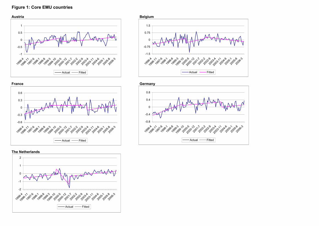
We now discuss the implications of the LMτ unit root tests regarding real
interest rate convergence in the EU area. We depict our findings in Figure 1. This
presents the (r – r*)t series calculated for all sample countries against the fitted
deterministic-trend values in each of the three-sub periods defined by the two breaks
points identified by our preferred minimum LM-test specifications.25 The deterministic-
trend values are given by the long-run solution for (r – r*)t obtained from the estimation
of the autoregressive model in equation (1) including a trend term.26
Starting from the EMU countries, an interesting distinction emerges between the
core and the periphery ones. In the former, RIRDs start from negative values and
converge towards zero during the run-up to the euro. Following the latter’s introduction,
breaks of differential effects are observed resulting, in positive RIRD trend values in
Germany and France, and negative RIRD trend values in Austria, Belgium and the
Netherlands. Finally, during the last sub-sample, deterministic trends in all countries
have shifted towards zero. Having said so, at the end of our sample period (2005) these
trends were set, with the exception of Belgium, towards positive RIRDs values.
The experience of periphery EMU countries is significantly different, the only
exception being Finland, whose real interest rate had converged to the EMU average by
the end of 2005. For the remaining countries, (Greece, Ireland, Italy, Portugal and
Spain) we initially observe substantial positive RIRD trend values. These were fast
reduced during the run-up to the euro, so that by the end of the first-sub sample they
were in negative territory. The only exception is Greece, where RIRD did not converge
to zero but actually increased further prior to euro’s introduction. Following the latter,
trend RIRD values in Ireland, Greece and Spain stabilized in negative levels, whereas in
25 For those countries where the null of unit root is maintained, the three sub-samples are defined by the
model accounting for breaks in both the level and the trend of the series. 26 The results do not change when linear trends are estimated directly using ordinary least squares.
15
Portugal and Italy they moved towards zero. Finally, at the end of our sample we
observe trends towards zero in Finland, Ireland, Portugal and Italy (although in the case
of the latter the LMτ test has maintained the null of unit root). On the other hand, trend
RIRD values are negative and declining in Greece and Spain.27
Moving on to the three opt-out EU countries, long-term trends towards RIP,
showing relatively little change over time, are observed in Denmark and Sweden, both
of which had converged to the EMU average by the end of 2005. An entirely different
picture is observed for the UK where (r – r*)t trends were consistently positive,
deviating from the RIP-consistent zero value throughout our sample.
Finally, and in relation to the new EU countries, leaving aside secondary
idiosyncrasies, four groups of countries emerge. The first consists of the Mediterranean
states of Cyprus and Malta where convergence is observed, with little structural change,
throughout the period under consideration. The second includes the Czech Republic,
Estonia and Slovakia where, generally speaking, RIRD trends were positive-increasing
during the first sub-period, positive-declining during the second sub-period; and
stabilized around zero during the third sub-period. The third consists of Lithuania and
Slovenia, where RIRD trends were positive-declining during the first sub-period,
increasing during the second, and converging towards zero during the third. The fourth
includes Latvia, Hungary and Poland, for which convergence is rejected. More
specifically, the LMτ test rejects the unit root hypothesis for Latvia, but at the same
time suggests a substantially negative trend differential at the end of our sample. On the
other hand, for Hungary and Poland, the unit root hypothesis is maintained and, at the
same time, substantially positive RIRD values are observed in recent years.
27 For Greece this is not so evident in Figure 1, due to the scale of the relevant diagramme caused by
some excessively positive RIRD values in the early years of our sample. The calculated RIRD series for
Greece over the period following the second identified structural break (2009.09-2006.03) has been
consistently negative with an average value equal to -0.27 per cent. On an annual basis, this is higher than
one percentage point.
16
5. SUMMARY AND CONCLUSION
This paper has tested the real interest parity (RIP) hypothesis in the EU25 area
making a two-fold contribution. First, we account for the effects of the previously
overlooked structural breaks in real interest rate differential (RIRD) series. Second, RIP
is tested for the first, to best of our knowledge, time against the EMU average. This
provides important insights relevant to the workings of the single currency and the
progress achieved by the new EU members towards joining it. Our analysis covers
1996-2005 (monthly data) and is based on ex-post RIRDs, calculated using identically
defined nominal and price inflation rates. Using the minimum Langrage Multiplier two-
break test developed by Lee and Strazicich (2003), we provide evidence generally in
favour of real interest rate convergence towards the EMU average. This, however, is a
gradual process, subject to structural breaks. Furthermore, convergence is rejected for a
small, but not negligible, number of countries.
Our convergence findings imply that for the majority of our sample countries the
steady-state costs of losing monetary independence should in principle be not too high,
especially for small countries whose ability to influence the EMU average real interest
rate would be minimal either within our outside the union. In the same spirit, and as RIP
is a comprehensive measure of economic integration, the convergence progress
achieved by the majority of the new EU countries indicates that these countries are now
significantly closer to joining the single currency than ten years ago.
These conclusions, however, may not apply in the short- and medium-run. As
convergence was found to be a quite heterogeneous and gradual, at best, process, the
loss of monetary independence may well imply sub-optimal economic stabilization in
individual countries (see e.g. Heinemann and Huefner 2004, Hayo and Hofmann, 2006).
This may be more than a merely transitory problem, as its welfare implications are
17
unknown and potentially significant. Addressing this question is not possible without
estimating an open-economy dynamic stochastic general equilibrium model capturing
the inter-temporal effects of ultimately transitory yet persistent deviations from RIP, a
task beyond the scope of the present paper. Having said so, and adopting a purely
financial point of view, it is plausible to argue that the observed heterogeneity in the
convergence process implies that risk-averse agents would have benefited from
diversifying their portfolios across EU countries rather than pursuing country-specific
investment strategies during the sample period covered by our analysis.
On the other hand, in countries such as Greece, Spain and Italy, rejection of
convergence implies that the adoption of the euro has caused asymmetric, relative to the
rest of the EMU members, monetary shocks. These may have resulted in less transitory,
and consequently more serious, economic costs such as bubbles in assets’ prices (see
e.g. Fernandez-Kranz and Hon 2006) and current account deterioration beyond the
degree justified by higher than EMU average economic growth (see e.g. Arghyrou 2006
and Arghyrou and Chortareas 2008). The experience of these countries suggests that
countries such as Latvia, Hungary, Poland and, perhaps most prominently, the UK,
where convergence was also rejected, adopting the euro in the foreseeable future may be
significantly more costly than in the rest of the current EMU outs.
Finally, a note relating to possible extensions of our work is due. Our findings
provide a solid platform to pursue further research on the question of real interest rate
convergence in Europe by means of investigating the specific factors underlying the
structural shifts in the RIRD series identified here. For example, the fast convergence
observed in periphery EMU countries during the run up to the euro may be due to a
reduction in a risk premium embodied in nominal interest rates but also, as we consider
ex-post real interest rates, faster than anticipated inflation reduction. In a similar
18
fashion, the negative trend-differential values observed following the launch of the euro
may reflect complete elimination of any previously existing risk premia as well as
higher than EMU average inflation rates, potentially reflecting productivity differentials
against the EMU average or a degree of incompatibility between the single monetary
policy and the macro-fundamentals of these countries. These questions could be
examined within a model of RIRD determination decomposing the latter’s movements
as the sum of factors such as those mentioned above. Constructing and estimating such
a model would provide us with further insights on the structural changes that have taken
place in our sample countries, the workings of the single monetary policy and the
welfare effects caused by euro participation.
REFERENCES
Alexakis, P., Apergis, N. and E. Xanthakis (1997), “Integration of international capital
markets: further evidence from EMS and non-EMS membership”, Journal of
International Financial Markets, Institutions and Money, 7, pp. 277-287.
Aksoy, Y., De Grauwe, P. and H. Dewachter (2002), “Do asymmetries matter for
European monetary policy?”, European Economic Review 46, pp. 443-469.
Arghyrou, M.G. (2006), “The effects of the accession of Greece to the EMU: Initial
Estimates”, Centre of Planning and Economic Research Study No 64, Centre of
Planning and Economic Research: Athens.
Arghyrou, M.G. and G. Chortareas (2008), “Current account imbalances and real
exchange rates in the Euro Area”, Review of International Economics,
forthcoming.
19
Arghyrou, M.G. and A. Gregoriou (2007), “Testing for Purchasing Power Parity
correcting for non-normality using the wild bootstrap”, Economics Letters, 95,
pp. 285-290.
Awad, M.A. and B.K. Goodwin (1998), “Dynamic linkages among real interest rates in
international capital markets”, Journal of International Money and Finance, 17,
pp. 881-907.
Bai, J. and P. Perron (2003), “Computation and analysis of structural change models”,
Journal of Applied Econometrics, 18, pp. 1-22.
Bayoumi, T. and B. Eichengreen (1993), “Shocking Aspects of European Monetary
Integration”, in F. Torres and F. Giavazzi (eds.), Adjustment and Growth in the
European Monetary Union: CEPR and Cambridge: Cambridge University Press
Cavaglia, S. (1992), “The persistence of real interest differentials: A Kalman Filtering
Approach”, Journal of Monetary Economics, 29, pp. 429-443.
Chinn, M.D. and J.A. Frankel (1995), “Who drives real interest rates around the Pacific
Rim: the USA or Japan?”, Journal of International Money and Finance, 14, pp.
801-821.
Cook, S. (2005), “The stationarity of consumption-income ratios: Evidence from
minimum LM unit root testing”, Economics Letters, 89, pp. 55-60.
Cumby, R. and M. Obstfeld (1984), “International interest rate and price level linkages
under flexible exchange rates: a review of recent evidence”, in Bilson J. and
R.C. Marston (eds.), Exchange Rate Theory and Practice, University of Chicago
Press, Chicago.
Dickey, D.A. and Fuller W.A. (1979), “Distribution of the Estimators for
Autoregressive Time Series with a Unit Root”, Journal of American Statistical
Association 74, pp. 427-431.
20
Dumas, B. (1992), “Dynamic Equilibrium and the Real Exchange Rate in Spatially
Separated World”, Review of Financial Studies, 5, pp. 153-80.
Dutton, M. M. (1993), “Real interest rate parity: new measures and tests”, Journal of
International Money and Finance, 14, pp. 801-825.
Edison, H. J. and B. D. Pauls (1993), “A re-assessment of the relationship between real
exchange rates and real interest rates: 1974-1990”, Journal of Monetary
Economics, 31, pp. 165-187.
Evans, L.T., Keef, S.P and Okunev, J. (1994), “Modelling real interest rates”, Journal of
Banking and Finance, 18, pp. 153-165.
Ferreira, A.L. and M.A. Leon-Ledesma (2007), “Does the real interest parity hypothesis
hold? Evidence for developed and emerging markets”, Journal of International
Money and Finance, 26, pp. 364-382.
Fernandez-Kranz, D. and M.T. Hon (2006), “A cross-section analysis of the income
elasticity of housing demand in Spain: Is there a real estate bubble?”, The
Journal of Real Estate Finance and Economics, 32, pp. 449-470.
Fountas, S. and J. Wu (1999), “Testing for real interest rate convergence in European
countries”, Scottish Journal of Political Economy, 46, pp. 158-174.
Frankel, J. (1979), “On the mark: the theory of floating exchange rates based on real
interest differentials”, American Economic Review, 69, pp. 610-622.
Frankel, J. and C. Okongwu (1995), “Liberalised portfolio capital inflows in emerging
markets: sterlization, expectations and the incompleteness of interest rate
convergence”, NBER Working Paper No 8828.
Fraser, P. and M. Taylor (1990), “Some efficient tests on international real interest
parity”, Applied Economics, 22, pp. 1083-1092.
21
Frenkel, J. (1976), “A monetary approach to the exchange rate: doctrine aspects of
empirical evidence”, Scandinavian Journal of Economics, 78, pp. 200-224.
Fujii, E. and Chinn, M.D. (2000), “Fin de siecle real interest parity”, NBER Working
Paper No 7880.
Galbraith, J.W. and V. Zinde-Walsh (1999), “On the distributions of Augmented
Dickey Fuller statistics in processes with moving average components”, Journal
of Econometrics 93, pp. 25-47.
Gagnon, J.E. and M.D. Unferth (1995), “Is there a world real interest rate?”, Journal of
International Money and Finance 14, pp. 845-855.
Goodwin, B.K. and T.J. Grennes (1994), “Real interest rate equalisation and the
integration of international financial markets”, Journal of International Money
and Finance, 13, pp. 107-124.
Hayo, B. and B. Hofmann (2006), “Comparing monetary policy reaction functions:
ECB versus Bundesbank”, Empirical Economics 31, pp. 654-662.
Heinemann, F. and F.P. Huefner (2004), “Is the view from the Eurotower purely
European? – National divergence and the ECB interest rate policy”, Scottish
Journal of Political Economy, 51, pp. 544-558.
Holmes, M.J. (2002), “Does long-run real interest parity hold among EU countries?
Some new panel data evidence”, The Quarterly Review of Economics and
Finance, 42, pp. 733-746.
Holmes, M.J. (2005), “Integration or independence? An alternative assessment of real
interest rate linkages in the European Union”, Economic Notes, 34, pp. 407-427.
Holmes, M.J. and N. Maghrebi (2006), “Are international real interest rate linkages
characterized by asymmetric adjustments?”, Journal of International Financial
Markets, Institutions and Money, 14, pp. 384-396.
22
Jorion, P. (1996), “Does real interest parity hold at longer maturities?”, Journal of
International Economics, 40, pp. 105-126.
Kugler, P. and K. Neusser (1993), “International real interest rate equalisation”, Journal
of Applied Econometrics, 8, pp. 163-174.
Koop, G. and S.M. Potter (2001), “Are apparent findings of nonlinearity due to
structural instability in economic time series”, The Econometrics Journal, 4, pp.
37-55.
Lee, J. and M.C. Strazicich, (2001), “Break point estimation and spurious rejections
with endogenous unit root tests”, Oxford Bulletin of Economics and Statistics,
63, pp. 535-558.
Lee, J. and M.C. Strazicich, (2003), “Minimum LM unit root test with two structural
breaks”, The Review of Economics and Statistics, 85, 1082-1089.
Lee, J., List, J.A. and M. C. Strazicich (2005), “Nonrenewable resource prices:
deterministic or stochastic trends?”, National Bureau of Economic Research,
Working Paper No 11487.
Lopez, J.H (1997), “The power of the ADF test”, Economics Letters, 57, pp. 5-10.
Lumsdaine, R. and D. Papell (1997), “Multiple trend breaks and the unit root
hypothesis”, Review of Economics and Statistics, 79, pp. 212-218.
MacDonald, R. and M.P. Taylor (1989), “Interest rate parity: some new evidence”,
Bulletin of Economic Research, 41, pp. 217-242.
MacKinnon, J.G (2002), “Bootstrap inference in econometrics”, Canadian Journal of
Economics 35, pp. 615-645.
Mancuso, J.A., Goodwin B.K and T.J. Grennes (2003), “Nonlinear aspects of capital
market integration and real interest rate equalization”, International Review of
Economics and Finance,12, pp. 283-303.
23
Mark, N.C. (1985), “Some evidence on the international equality of real interest rates”,
Journal of International Money and Finance, 4, pp. 189-208.
Marston, R.C. (1995), International Financial Integration: A study of interest
differentials between the major industrial countries, Cambridge University
Press.
Meese, R. and K. Rogoff (1988), “Was it real? The exchange rate-interest differential
relation over the modern floating-rate period”, The Journal of Finance, 43, pp.
933-948.
Mishkin, F.S. (1984a), “Are real interest rates equal across countries? An empirical
investigation of international parity conditions”, The Journal of Finance, 39, pp.
1345-1357.
Mishkin, F.S. (1984b), “The real interest rate: a multi-country empirical study”,
Canadian Journal of Economics 17, pp. 283-311.
Moosa, I. and R. Bhatti (1996), “Some evidence on mean reversion in ex ante real
interest rates”, Scottish Journal of Political Economy, 43, pp. 177-191.
Mussa, M.L. (1982), “A model of exchange rate dynamics”, Journal of Political
Economy, 90, pp. 74-104.
Nakagawa, H. (2002), “Real exchange rates and real interest rate differentials:
implications of nonlinear adjustment in real exchange rates”, Journal of
Monetary Economics, 49, pp. 629-649.
Nunes, L., Newbold, P. and C.M. Kuan (1997), “Testing for unit roots with breaks:
Evidence on the great crash and the unit root hypothesis reconsidered”, Oxford
Bulletin of Economics and Statistics, 59, pp. 435-448.
Obstfeld, M. and A.M. Taylor (2002), “Globalisation and capital markets”, NBER
Working Paper No 8846.
24
Ong, L.L., Clements, K.W. and H.Y. Izan (1999), “The world real interest rate:
stochastic index number perspectives”, Journal of International Money and
Finance, 18, pp. 225-249.
Perron, P. (1989), “The Great Crash, the oil price shock and the unit root hypothesis”,
Econometrica, 57, pp. 1361-1401.
Perron, P. (1997), “Further evidence on breaking trend functions in macroeconomic
variables”, Journal of Econometrics, 80, pp. 355-385.
Phylaktis, K. (1999), “Capital market integration in the Pacific Basin Region: an
impulse response analysis”, Journal of International Money and Finance, 18,
pp. 267-287.
Strazicich, M.C., Lee, J. and E. Day (2004), “Are incomes converging among OECD
countries? Time series evidence with two structural breaks”, Journal of
Macroeconomics, 26, pp. 131-145.
Wu, J.L. and S.L. Chen (1998), “A re-examination of real interest rate parity”,
Canadian Journal of Economics, 31, pp. 837-851.
Van Dijk, D., Franses, P.H. and A. Lucas (1999), “Testing for smooth transition
nonlinearity in the presence of outliers”, Journal of Business & Economic
Statistics, 17, pp. 217-235.
Zivot, E. and D.W.K. Andrews (1992), “Further evidence on the Great Crash, the oil
price shock and the unit root hypothesis”, Journal of Business and Economic
Statistics, 10, pp. 251-270.
25
APPENDIX
A potential source of bias in standard ADF analysis is violations of the
assumptions of normality and heteroscedasticity under which the critical values of the
ADF test have been derived. In a recent paper Arghyrou and Gregoriou (2007) address
this problem using a wild bootstrap simulation technique. This entails estimation of a
new series given by:
(rt - r*)′t = (rt - r*)t ut (1A)
where tu is drawn from the two-point distribution
0.5
0.50.5
0.5
1 5(5 1)/2 with probability
2(5 )
(5 1)/2 with probability (1 )
p
t pu
+
+− − =
−
(2A)
The tu terms are mutually independent drawings from a distribution
independent of the original data characterised by the properties 0)( =tuE , )( 2tuE =1
and )( 3tuE = 1. Hence, any non-normality/heteroscedasticity in rt is preserved in the
created series (rt - r*)′t . We generate 10,000 sets of (rt - r*)′t series. Subsequently, for
each bootstrap iteration, a series of DF tests is constructed under the null hypothesis
φ = 0. Therefore the generated sequence of artificial data has a true φ coefficient of
zero. However, when we regress the artificial DF test for a given bootstrap sample 0t
estimated values of φ that differ from zero will result. This procedure provides an
empirical distribution for φ and their associated standard errors based exclusively on the
re-sampling of the original series (rt - r*)′t. Therefore appropriate critical values are
obtained for the null hypothesis of unit root (φ̂ = 0) in equation (2). The results of this
bootstrap experiment are reported in column (c) of Table 2 and discussed in section 4.1.
Table 1: Descriptive statistics of real interest rate differentials against the EMU average (r-r*)
Mean Std Deviation Normality Correlation coefficient
between r and rEMU EMU countries Austria 0.02 0.27 0.05* 0.73 Belgium -0.05 0.37 0.18 0.66 Finland 0.04 0.35 0.00** 0.53 France 0.01 0.18 0.87 0.90 Germany 0.05 0.25 0.06+ 0.79 Greece 0.55 1.19 0.00** 0.63 Ireland -0.18 0.48 0.38 0.72 Italy 0.11 0.38 0.00** 0.83 Netherlands -0.20 0.41 0.00** 0.31 Portugal -0.24 0.51 0.10 0.45 Spain -0.15 0.34 0.06+ 0.87 Average 0.00 0.43 N/A 0.67
Opt-out EU countries Denmark 0.01 0.30 0.05* 0.66 Sweden 0.20 0.40 0.17 0.63 UK 0.59 0.28 0.43 0.71 Average 0.27 0.33 N/A 0.67
New EU countries Cyprus 0.11 0.84 0.25 0.37 Czech Rep. 0.44 0.89 0.00** 0.56 Estonia -0.07 1.20 0.00** 0.28 Hungary 0.94 0.75 0.49 0.32 Latvia -0.36 0.76 0.03* 0.55 Lithuania 0.31 0.96 0.00** 0.50 Malta -0.02 0.55 0.07+ 0.34 Poland 1.65 1.04 0.23 0.64 Slovakia 0.58 1.75 0.38 0.50 Slovenia -0.20 0.84 0.00** 0.36 Average 0.34 0.96 N/A 0.44
Notes: +, *, ** respectively denote statistical significance at the 10, 5 and 1 per cent level. Normality is the p-value of the Normality Chi-square Bera-Jarque test for non-normality.
Table 2: Unit root tests: Augmented Dickey Fuller and Perron (1997)
(a)
ADF with
constant only
(b)
ADF with
constant and trend
(b)
Wild bootstrap analysis:
Lower limits of confidence interval
(d)
Perron (1997) single break test
with shift in constant
(e)
Perron (1997) single break test with shift in constant and trend
Notes: +, *, ** respectively denote statistical significance at the 10, 5 and 1 per cent level. The lower limits of the reported wild bootstrap critical values are the critical values of the ADF test corrected for heteroscedasticity/non-normality. The statistical significance of the Perron (1997) t-scores is determined using the test’s critical values corrected for small samples (100 observations).
Table 2 (continued): Unit root tests: Lee and Strazicich (2003)
(f)
Lee and Strazicich (2003) test
Breaks in constant
(g)
Lee and Strazicich (2003) test Breaks in constant and trend
LMτ-score Break 1 Break 2 LMτ-score Break 1 Break 2 EMU countries Austria -6.24 [5]** 1998:04 2003:12 -6.96 [5]** 2000.03 2003.08 Belgium -5.56 [8]** 1999.06 1999.12 -8.15 [8]** 1999.12 2002.01 Finland -2.37 [3] 2001.03 2004.02 -5.92 [11]* 1999.03 2003.11 France -5.25 [5]** 2001.08 2003.01 -6.73 [5]** 1999.01 2003.01 Germany -3.67 [8]+ 1997.12 2003.01 -5.74 [8]* 1999.07 2003.10 Greece -4.21 [2]* 1997.08 2005.03 -11.38 [0]** 1997.10 2000.09 Ireland -3.29 [3] 1997.10 1999.08 -5.86 [10]* 1999.10 2003.03 Italy -3.12 [11] 2001.12 2004.04 -4.65 [11] 1997.08 2000.06 Netherlands -3.85 [11]* 1999.07 2000.11 -6.61[2]** 1999.10 2001.03 Portugal -3.27 [9] 2001.12 2003.06 -5.76 [11]* 2000.09 2004.05 Spain -4.69 [10]** 1998.06 2000.04 -5.54 [10]+ 1998.05 2000.06 Opt-out EU countries Denmark -4.75 [11]** 1997.06 2005.02 -7.19 [11]** 1997.12 2004.07 Sweden -4.13 [11]* 2003.03 2004.04 -5.68 [11* 2000.01 2004.02 UK -4.47 [5]* 1997.06 2000.10 -5.87 [5]* 2000.09 2003.11 New EU countries Cyprus -3.41 [10] 1998.01 2001.06 -6.07 [10]* 1998.12 2000.04 Czech Rep. -3.35 [9] 1997.08 1998.03 -5.92 [9]* 1997.12 1999.11 Estonia -1.40 [7] 1998.04 2003.06 -6.02 [10]* 1999.03 2001.03 Hungary -2.83 [11] 1997.09 2002.11 -4.64 [5] 1998.04 2000.10 Latvia -4.43 [5]* 2002.08 2004.06 -5.50 [10]+ 1998.10 2003.08 Lithuania -5.09 [5]** 2000.05 2003.03 -5.57 [5]+ 2000.05 2004.01 Malta -6.12 [5]** 1998.06 2001.01 -6.75 [5]** 2001.02 2001.12 Poland -2.58 [9] 1998.07 1999.06 -4.63 [10] 1998.11 2001.01 Slovakia -4.53 [4]* 2000.01 2000.07 -5.57 [4]+ 1998.12 2000.01 Slovenia -5.42 [5]** 1999.07 2000.10 -5.96 [1]* 1997.06 2002.05 Notes: +, *, ** respectively denote statistical significance at the 10, 5 and 1 per cent level. Bold letters indicate the preferred specification of the minimum LM-unit root test, determined by the strongest rejection of the null. The selected models remain robust when selection is undertaken using the Akaike information criterion (results available upon request). Statistical inference is drawn by comparing the LMτ tests reported in columns (f) and (g) with the critical values reported taken in Table 2 in Lee and Strazicich (2003), for Models A and C (II) respectively.