The Real Exchange Rate, Real Interest Rates, and the Risk Premium 

  

Charles Engel 

1

University of Wisconsin 

Define the excess return or “risk premium” on Foreign s.t. bonds:  

* *1 1t t t t t t t t t t ti E s s i r E q q rλ + +≡ + − − = + − −  

 The famous Fama regression demonstrates that as  −*

tr tr  falls, λt  falls ‐ I verify this for real rather than nominal interest rates  On the other hand, as  −*

tr tr  falls (i.e.,  − *tr tr  rises), Home currency 

appreciates “excessively” – more than can be explained by expectations of future interest rates under UIP  

Are these two findings:  

λ− − <*cov( , ) 0t t tr r  − − <*cov( , ) 0IP

t t t tq q r r   

2

arising from the same source?

 No.  They seem to say the opposite.  

λ− − <*cov( , ) 0t t tr r   means when home   is high (relative to  , relative to average), home deposits are riskier. 

tr*tr

 − − *cov( , ) 0IP

t t t tq q r r <  

3

means when home   is high (relative to  , relative to average), the home currency is stronger than it would be under interest parity.  Why? Because home deposits are less risky. 

tr*tr

  1.  Empirical methodology  2.  Empirical results 3.  Why findings are a puzzle   ‐‐ not readily explainable by complete‐market risk‐premium models   ‐‐ not readily explainable by “delayed overshooting” models 

4

4.   Type of model that resolves puzzle. 

Real interest rates and real exchange rates.  Rewrite:   *

1 ( ) ( )t t t t t tq E q r r r λ λ+− = − − − − −   Iterate forward to get:  

   ( )limt t t j t tjq E q R+→∞− = − −Λ

where   

 *

0

( )t t t j t jj

R E r r r∞

+ +=

≡ − −∑     0

( )t t t jj

E λ λ∞

+=

Λ ≡ −∑  

 

tΛ  ‐ “level risk premium”  We find evidence for long run purchasing power parity: lim t t jj

E q q+→∞=  

5

= −ΛIPt t tq q  

 Data  U.S., Canada, France, Germany, Italy, Japan, U.K., and “G6”  G6 is like doing panel regressions  Exchange rates – last day of month (noon buy rates, NY) Prices – consumer price indexes Interest rates – 30‐day Eurodeposit rates (last day of month)  Monthly, June 1979 – October 2009   

6

 

VAR methodology Two different VAR models:  Model 1:  * * *

1 1, , ( )t t t t t t tq i i i iπ π− −⎡ ⎤− − − −⎣ ⎦   Model 2:  * *, ,t t t t tq i i π π⎡ ⎤− −⎣ ⎦   (Extensions include long‐term bond yields and stock returns.)  Estimate VAR with 3 lags.  (Extension with 12 lags.)  Use standard projection measures to estimate 

*1)

* *1(t t t t t t t tr r i i E Eπ π+− = − − − + ,  and  

∞

+ +=

≡ − − − +∑ *

0

( )IPt t t j t j

j

q E r r r q  

 Then  tλ  is constructed as   r*

1t t t t t tr E q qλ +≡ + − −  

7

tΛ  estimate is constructed from Λ = −IPt t tq q  

Fama Regression in Real Terms:  ζ β+ +− − = − − +1 , 1ˆ ˆd dt t t q q t qq q r r u t  

Country  1̂β   90% c.i.(  1̂β ) 

8

Canada  0.862  (‐0.498,2.222) (‐0.632,2.908) (‐0.676,2.800) 

France  1.576  (‐0.117,3.269) (0.281,3.240) (‐0.125,3.602) 

Germany  1.837  (‐0.015,3.689) (0.687,4.458) (0.589,4.419) 

Italy  0.360  (‐1.336,2.056) (‐1.087,2.136) (‐1.358,2.328) 

Japan  2.314  (0.768,3.860) (0.746,4.300) (0.621,4.441) 

United Kingdom  2.448  (0.854,4.042) (0.873,4.614) (1.039,4.846) 

G6  1.933  (0.318,4.548) (0.510,3.932) (0.473,4.005) 

Regression of  on tq   *ˆ ˆt tr r− :  *0 1 1ˆ ˆt t tq uβ β ( )tr r += + − +  

1̂β   90% c.i.(  1̂β )Country   Canada 48.517 (‐62.15,‐34.88) 

( .4    ‐  

‐94.06,‐31 1)(‐140.54,‐27.34) 

France  ‐20.632  (‐32.65,‐8.62) (‐44.34,‐1.27) (‐54.26,1.75) 

Germany  ‐52.600   (  (‐67.02.‐38.18)‐85.97,‐25.35)

(‐105.29,‐19.38) Italy  ‐39.101  (‐51.92,‐26.28) 

(‐67.63,‐16.36) (‐90.01,‐13.70) 

Japan  ‐19.708  (‐29.69,‐9.72) (‐42.01,‐1.05) (‐46.53,‐4.33) 

United Kingdom  ‐18.955  (‐31.93,‐5.98) (‐40.19,‐3.08) (‐55.94,4.08) 

G6  ‐44.204   (  

9

(‐55.60,‐32.80)‐73.17,‐23.62)(‐82.87,‐21.74) 

ˆtΛ  on  *ˆ ˆt tr r− : *

0 1 1ˆ ˆ ˆ(t tr rβ )t tuβ +Λ = +  + −Regression of   

Country 1̂β   90% c.i.(  1̂β ) 

Canada  0  (15.12,32.10) 9

 

23.61(12.62,51. 6) (11.96,63.71)

France  13.387  (1.06,25.72) (‐2.56,36.25) (‐6.98,42.40) 

Germany  34.722  (19.66,49.78) (9.34,57.59) (3.68,69.36) 

Italy  27.528  (17.58,37.48) (14.98,48.32) (12.51,58.54) 

Japan  15.210  (4.76,25.66) (‐0.45,37.08) (0.91,38.87) 

United  

10

 Kingdom 14.093  (0.33,27.86) (0.39,34.46) (‐8.70,46.45) 

G6  31.876  (20.62,43.13) (16.89,54.62) (16.78,60.89) 

Implications:  

*cov( , ) 0r rt t tλ − <   (Fama regression in real terms)  

* *ov( , ) 0t t j t tE r rλ0

cov( , ) ct t tj

r r∞

=

Λ − = ∑ + − >   (from VAR estimates) 

→  

*cov( , ) 0t t j t tE r rλ + − >  for some j (as i xplaining 

n previous figure) 

E *cov( , ) 0t tr rtλ − <  and  *cov( , ) 0E r rt t j t tλ − >  +

ris  when  *

is a challenge for 

k premium models – t tr r−  is high, the home currency is both riskier than average and expected to be less risky than average. 

11

 Notation:   + += −1 1t t td q q  

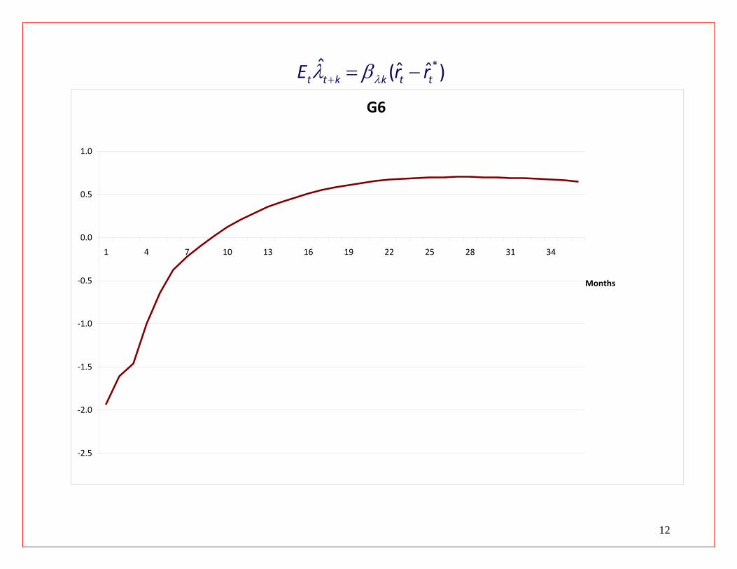
  *ˆ ˆ ˆ( )t t k k t tE r rλλ β+ = −

12

G6

‐2.5

‐2.0

‐1.5

‐1.0

‐0.5

0.0

0.5

1.0

1 4 7 10 13 16 19 22 25 28 31 34

Months

 

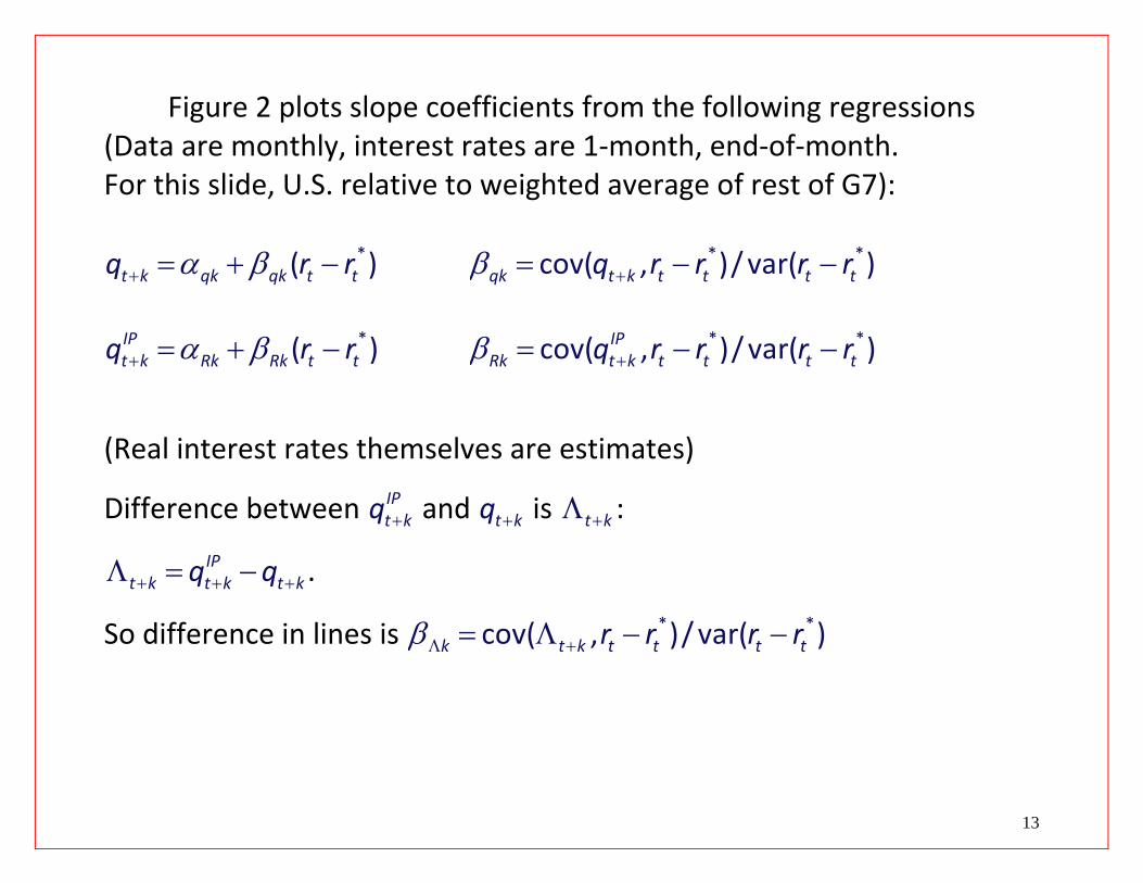
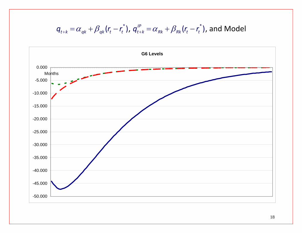
Figure 2 plots slope coefficients from the following regressions (Data are monthly, interest rates are 1‐month, end‐of‐month. For this slide, U.S. relative to weighted average of rest of G7):  

*(t k qk qk t tq r )rα β+ = + −     * *cov( , )/ var( )qk t k t t t tq r r r rβ += − −   

α β+ = + − *(IPt k Rk Rk t tq r )r     β += − −* *cov( , )/ var( )IP

Rk t k t t t tq r r r r   

(Real interest rates themselves are estimates) 

Difference between  +IPt kq  and  ktq +  is  t k+Λ : 

+ +Λ = −IPt k t k t kq q + . 

13

So difference in lines is  * *cov( , )/ var( )k t k t t t tr r r rβΛ += Λ − −  

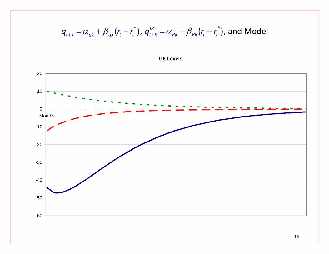
*( )t k qk qk t tq r rα β+ = + − ,  α β+ = + − *( )IPt k Rk Rk t tq r r  

14

G6 Levels

-50.000

-45.000

-40.000

-35.000

-30.000

-25.000

-20.000

-15.000

-10.000

-5.000

0.000Months

 

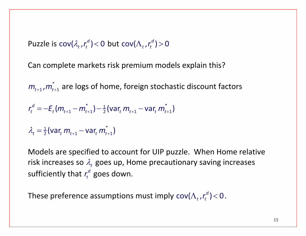
Puzzle is  λ <cov( , ) 0dt tr  but  Λ >cov( , ) 0d

t tr   Can complete markets risk premium models explain this?  

*1 ,tm m+ 1t+  are logs of home, foreign stochastic discount factors  

 * *1

1 1 1 12( ) (var var )dt t t t t t t tr E m m m m+ + + +  = − − − − 

*11 12 (var var )t t t t tm mλ + += −  

 Models are specified to account for UIP puzzle.  When Home relative risk increases so λt

dt

 goes up, Home precautionary saving increases sufficiently that   goes down. r 

15

These preference assumptions must imply  Λ <cov( , ) 0dt tr . 

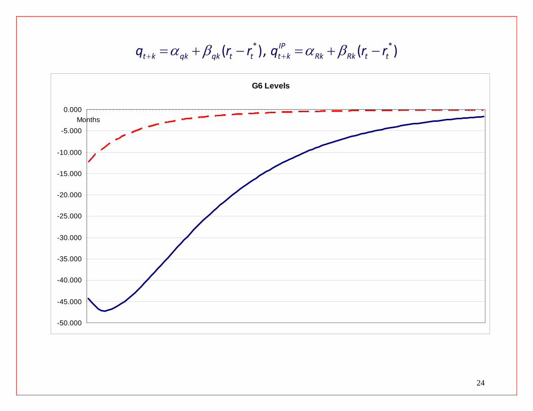
*( )t k qk qk t tq r rα β+ = + − ,  α β+ = + − *(IPt k Rk Rk t tq )r r , and Model 

 

16

G6 Levels

-60

-50

-40

-30

-20

-10

0

10

20

Months

Delayed overshooting to monetary shocks has been explained in models of delayed reaction in the foreign exchange market Froot and Thaler (1990), Bacchetta and van Wincoop (2010)  The impulse response function for   starts off negative, declines for awhile, and then increases. 

tq

 Model can give us  λ <cov( , ) 0d

t tr , and even  + <1cov( , ) 0dt td r ,  

  but implies  Λ <cov( , ) 0dt tr  

 

17

The real exchange rate underreacts to the increase in real interest rates, rather than overreacting. 

*( )t k qk qk t tq r rα β+ = + − ,  α β+ = + − *(IPt k Rk Rk t tq )r r , and Model 

 

18

G6 Levels

-50.000

-45.000

-40.000

-35.000

-30.000

-25.000

-20.000

-15.000

-10.000

-5.000

0.000Months

Models with a single economic variable driving   and dtr λt : 

 

  ε∞

−=

=∑0

dt j

j

r a t j     λ ε∞

−=

=∑0

t j t jj

c  

 1.  Single factor models:  λ=d

t tr k   2. Unidirectional models:   same sign ja ∀j , and   same sign ∀j . jc These are common assumptions.  Sometimes both are made.  Assumption 2, especially, seems sensible.  Theorem: we cannot get  λ <cov( , ) 0d

t tr  and  Λ > 0cov( , )dr   t t

 

19

Need at least two shocks.  One must matter in short run and deliver λ <d .  The other must be more persistent and have cov( , ) 0t trλ + >cov( , )dt t j tE r 0 in order to get  Λ >cov( , ) 0d

t tr .

An example of a model that would work:  Standard New Keynesian, except u.i.p. does not hold (good starting place because of implications under u.i.p.):  Open‐economy Phillips curve: π π δ β π π+ +− = + −* *

1 1( )t t t t t tq E  Taylor rule: 

σ π π ε− +* *( )t t t ti i− = t ,  εε ρ ε ς−= +1t t t   “Liquidity” premium – short‐term bonds have value as collateral λ α π π+ += − − − −⎣ ⎦

* *1 1( )t t t t t t ti E i E ηt ,   ⎡ ⎤ α > 0  

ηt  ‐‐ exogenous increase in value of Foreign bonds  

20

α π +⎡ ⎤− − −⎣* *

1 (t t t t t ti E i E π + ⎦1)  ‐‐ Home bonds are more valued as collateral 

during Home monetary policy contraction 

This can account for  1cov( , ) 0dt t tE d r+ <  and   when Λ >cov( , ) 0d

t tr ηt  is more volatile but less persistent than αεt .  λ α π π η+ +⎡ ⎤= − − − −⎣ ⎦

* *1 1( )t t t t t t t ti E i E

 η ↑t    Foreign assets more valuable.  Foreign currency appreciates, increasing inflationary pressure in Home.     

⇒⇒ ↑d

tr .     This tends to give us  λ <cov( , ) 0d

t tr  and  1cov( , ) 0dt t tE d r+ <  as in u.i.p. 

puzzle   ε ↑t    Home monetary contraction, ⇒ ↑d

tr .  Relative liquidity value of Home assets rises, tends to make  λ >cov( ) 0, d

t tr .  If ηt  is more volatile, it dominates short run behavior of  λcov( , )dt tr .  If ε t  is sufficiently persistent, it dominates long run behavior and determines 

Λ d . cov( , )t tr

21

 

 ε

ε ε ε

α ρ β ε ηδ α σ ρ ρ β ρ σδ α

− + −= +

+ − + − − + +(1 )(1 ) 1

(1 )( ) (1 )(1 ) 1 (1 )t t tq  

 

ε ε

ε ε ε

α ρ β ρ σδλ ε ηδ α σ ρ ρ β ρ σδ α

− − +⎛ ⎞= −⎜ ⎟+ − + − − + +⎝ ⎠

(1 )(1 ) 1(1 )( ) (1 )(1 ) 1 (1 )t t t  

 

ε

ε ε ε

α ρ β σδε ηδ α σ ρ ρ β ρ σδ α

− +⎛ ⎞Λ = −⎜ ⎟+ − + − − + +⎝ ⎠

(1 ) 1(1 )( ) (1 )(1 ) 1 (1 )t t t  

 

22

ε ε

ε ε ε

ρ β ρ σδε ηδ α σ ρ ρ β ρ σδ α

− −= +

+ − + − − + +(1 )(1 )

(1 )( ) (1 )(1 ) 1 (1 )dt t tr

Conclusions:  

A new puzzle.  Our models for the UIP puzzle don’t seem adequate.    Visually, the finding of  Λ >cov( , ) 0d

t tr  may be more important than the UIP puzzle,  λ <cov( , )dt tr 0.    Understanding this matters:    1.  For understanding exchange rates 

23

  2.  For understanding macroeconomics and finance. 

24

*( )t k qk qk t tq r rα β+ = + − ,  α β+ = + − *( )IPt k Rk Rk t tq r r  

G6 Levels

-50.000

-45.000

-40.000

-35.000

-30.000

-25.000

-20.000

-15.000

-10.000

-5.000

0.000Months