Do Taxpayers Bunch at Kink Points?

By Emmanuel Saez∗

August 2, 2009

Abstract

This paper uses individual tax return micro data from 1960 to 2004 to analyze whethertaxpayers bunch at the kink points of the U.S. income tax schedule generated by jumps inmarginal tax rates. We develop a method to estimate the compensated elasticity of reportedincome with respect to (one minus) the marginal tax rate using bunching evidence. Wefind clear evidence of bunching around the first kink point of the Earned Income TaxCredit with implied estimated intensive earnings elasticity around 0.25. The response isconcentrated among those with self-employment income with elasticities around one andgrows overtime. Elasticities are always equal to zero for wage earners. A simple tax evasionmodel can account for those results. We find evidence of bunching at the threshold of thefirst tax bracket where tax liability starts, especially in the 1960s when the tax schedulewas stable and simple. However, there is no evidence of bunching at all for other kinkpoints of the tax schedule, even when the tax brackets are stable over many years andwhere jumps in marginal tax rates are substantial. (JEL H24, H31)

A large body of empirical work in labor and public economics analyzes the behavioral

response of earnings to taxes and transfers using the standard static model where agents

choose to supply hours of work until the marginal disutility of work equals marginal utility of

disposable (net-of-tax) income.1 This model, which from now on we call the standard model,

predicts that, if individual preferences are convex and smoothly distributed in the population,

we should observe bunching of individuals at convex kink points of the budget set. Taxes

and government transfers create such kink points. The progressive US individual income

tax generates a piece-wise linear budget set with kinks at each point where the marginal∗University of California, Department of Economics, 549 Evans Hall #3880, Berkeley CA 94720, USA (e-mail:

saez@econ.berkeley.edu). This paper builds upon an initial NBER working paper Saez (1999), subsequentlyrevised for the NBER-TAPES 2002 conference but never published. I thank two anonymous reviewers, RichardBlundell, Raj Chetty, Peter Diamond, Esther Duflo, Dan Feenberg, Roger Gordon, Jonathan Gruber, RogerGuesnerie, Jerry Hausman, Jeffrey Liebman, Costas Meghir, Bruce Meyer, James Poterba, Ian Preston, ToddSinai, and TAPES conference participants for helpful comments and discussions. Financial support from theAlfred P. Sloan Foundation and NSF Grant SES-0850631 is thankfully acknowledged.

1Martin Feldstein (1999) shows that this model can be extended to analyze not only the choice of hours ofwork but more generally the response of overall income to marginal tax rates.

tax rate jumps. Means-tested government transfer programs also introduce piecewise-linear

constraints because transfer benefits are “taxed” away as income rises. In particular, the

Earned Income Tax Credit (EITC) creates two large convex kink points at the points where the

credit is fully phased-in, and where it starts being phased-out. Looking for bunching evidence

around kinks provides a simple test of the widely used standard model and of the presence

of behavioral responses to taxation along the intensive margin. Furthermore, the amount of

bunching generated by budget set kinks is proportional to the size of the compensated elasticity

of income with respect to the net-of-tax rate.

The present paper has therefore two goals. First, we investigate thoroughly whether there

is evidence of bunching at the kink points of the US federal income tax–and in particular at the

large kink points created by the EITC. Second, we develop an econometric method to estimate

compensated elasticities of reported income with respect to net-of-tax rates using bunching

evidence. Our empirical analysis uses the large annual tax return data publicly released by

the Internal Revenue Service (IRS) since 1960. Those administrative data are ideally suited

for the analysis because they provide information about the exact location of taxpayers on the

tax schedule and, in contrast to standard survey data, have almost no measurement error. We

obtain three main empirical results.

First, we find clear evidence of bunching around the first kink point of the EITC–the point

at which the credit reaches its maximum level–with an implied elasticity of earnings around

0.25. Such bunching evidence constitutes perhaps the most compelling evidence to date of

behavioral responses created by the EITC along the intensive margin.2 However, we find

that bunching is concentrated among EITC recipients with self-employment income with a

very large implied elasticity around one. EITC recipients with only wage earnings display no

evidence of bunching and thus the implied elasticity for wage earners is zero and precisely

estimated. This suggests that most of the bunching response might be due to reporting effects

rather than real labor supply effects.3 We develop a simple model of reporting which can2A large body of work has shown strong evidence of behavioral responses to the EITC along the extensive

margin, i.e. the decision to participate in the labor force. Evidence of behavioral responses along the intensivemargin (i.e., hours of work conditional on working) is weak or absent (see Nada Eissa and Hilary Hoynes (2006)and V. Joseph Hotz and John Karl Scholz (2003) for recent surveys).

3Those results are consistent with the recent and complementary analysis by Sara Lalumia (2009) whichshows that EITC expansions lead to an increase in the fraction of low income filers with children reportingself-employment income.

1

account for our empirical findings. Furthermore, the amount of bunching grows overtime (the

EITC schedule has been stable since the major expansion of 1993-1996) perhaps because tax

filers learn slowly about the EITC schedule. Second, we also find evidence of bunching at the

threshold of the first tax bracket where tax liability starts, especially in the 1960s when the tax

schedule was stable and very simple. The implied elasticities are also significant in that case,

around 0.2. Part of the elasticity is due to the response of itemized deductions as the evidence

of bunching is not as sharp for taxable income recomputed using always the standard deduction

(instead of the maximum of the standard deduction and itemized deductions). Third, however,

we cannot find any bunching evidence for other kink points of the tax schedule, even when

jumps in marginal tax rates are large and stable over many years, and even when restricting

the sample to more responsive sub-groups such as those reporting self-employment income.

Therefore, our evidence shows that taxpayers behave as in the standard labor supply model

only in very specific cases. The first kink of the EITC is special because it is the level of earnings

that maximizes the tax refund any should indeed be the focal point for tax filers mis-reporting

their incomes. The first kink point of the income tax schedule is the income level where tax

liability starts and hence might be more visible on tax tables than kink points at higher income

levels. Indeed, survey evidence suggests that many taxpayers do not know their marginal tax

rate or report it with substantial error (see e.g., Edwin T. Fujii and Clifford B. Hawley, 1988

for US evidence).

Our analysis relates to the nonlinear budget set labor supply estimation method.4 This

method was originally developed to address the endogeneity of the marginal tax rate to the

labor supply choice (as higher labor supply may push the individual into a higher tax bracket).

In that context, nonlinear budget sets created by the tax system were seen as a source of endo-

geneity problems which had to be solved using a structural model rather than an opportunity

to identify behavioral responses to taxation as in our analysis of bunching.

No study has carefully examined the evidence of bunching at the kink points of the US

income tax schedule to uncover evidence of behavioral responses, in spite of data availability.5

4First developed by Gary Burtless and Jerry Hausman (1978) to study the Negative Income Tax experiments,Hausman (1981) applied the method to study the effect of the US income tax on labor supply. Robert Moffitt(1986, 1990) provides a survey of the method and its many subsequent applications.

5US tax return data have been available for a long time but rarely used by labor economists. As pointed outby Hausman (1982), in defense of the nonlinear budget set methods and in response to a criticism by JamesHeckman (1982) who argued that no bunching evidence could be found in the data, survey data have too much

2

A recent study by Raj Chetty et al. (2009) uses tax return data from Denmark and uncovers

substantial bunching at a large kink point of the Danish income tax schedule where the top

rate starts to apply. This kink point is simple and salient because it is large and the same for

all individuals.6 Consistent with our US results, they do not find much evidence of bunching

at smaller kink points of the Danish tax schedule.

A few other studies have documented evidence of bunching at the kink points generated by

other government programs. First, Burtless and Moffitt (1984) and Leora Friedberg (2000),

using Current Population Survey data, observed bunching behavior in the case of elderly

individuals who receive social security benefits but are still working and subject to the Social

Security earnings test.7 Those studies however do not use bunching to estimate compensated

elasticities as we do here. They instead rely on the standard nonlinear budget set method

for estimating behavioral responses. Second, Richard Blundell and Hoynes (2004) document

clear evidence of bunching at exactly 16 hours per week for individuals likely to be eligible

for the UK family credit which imposes a 16 hour minimum working requirement. Finally,

pension programs also generate kinks (or cliffs) in the lifetime budget set. As is well known,

retirement hazard rates display bunching at certain ages related to the parameters of the

retirement programs8 Those studies point out that bunching is evidence of behavioral responses

to pension programs although they do not directly use bunching to estimate elasticities. A

recent notable exception is Kristine Brown (2007) who uses changes in the kink points due

to reforms in the California Teachers retirement program to estimate elasticities of retirement

age with respect to price incentives. In contrast to our study, Brown (2007) uses reforms and

corresponding changes in bunching behavior to estimate elasticities while we focus on a more

basic cross-sectional estimation method.

The paper is organized as follows. Section I presents the conceptual framework, the data,

and discusses the estimation methodology. Section II presents the EITC based results. We

measurement error to study bunching precisely.6Chetty et al. (2009) argue that part of the bunching might be driven by employers’ pay policies which are

tailored to avoid the top bracket, which is feasible in Denmark as the top bracket threshold is uniform acrossall individuals and taxes are based on individual income (as opposed to family income as in the United States).

7Social security benefits are taxed away (actually deferred) when earned income exceeds an exemptionamount. Tax rates vary from 33 percent to 50 percent and thus generate substantial kinks in the budget set ofthe elderly. This phasing-out structure is simple and hence likely to be salient to social security beneficiaries.

8For example, in the United States, there is bunching at the early retirement age of 62 (when workers becomeeligible to claim Social Security benefits) and bunching at the normal retirement age (see Jonathan Gruber andDavid A. Wise (1999) for an analysis across a number of countries).

3

start with the EITC analysis because the EITC creates the largest kinks in the budget con-

straint and this is precisely where the bunching evidence is most striking. Section III then

presents results based on the regular federal income tax schedule where bunching evidence is

much weaker. Section IV concludes.

1 Model, Data, and Methodology

1.1 Standard Model and Small Kink Analysis

We consider the standard model with two goods where individuals’ utility functions depend

positively on after-tax income c (individuals value consumption) and negatively on before-tax

income z (earning income requires effort). We assume that, with a linear budget set with

constant marginal tax rate t, individual incomes z are distributed according to a smooth

density distribution h(z). The heterogeneity in earnings z is due to differences in preferences

or ability–both of which are captured by heterogeneity in the utility function u(c, z) across

individuals.

Suppose that a (small) kink is introduced in the budget set at income level z∗ by increasing

the marginal tax rate from t to t + dt for incomes above z∗ as depicted on Figure 1A. Such

a kink is going to produce bunching of individuals whose incomes were falling into a segment

[z∗, z∗+dz∗] before the kink was introduced as displayed on Figure 1B. The individual (denoted

by L on Figure 1A) with earnings z∗ before the tax change is not affected and his indifference

curve remains tangent to the lower part of the budget set (with slope 1− t). Let us denote by

H the highest income earner (before the tax change) who is now bunching at the kink. Before

the tax change, individual H had earnings z∗ + dz∗ and his indifference curve was tangent to

the linear budget with slope 1− t as shown in Figure 1A. After the tax change, his indifference

curve is exactly tangent to the upper part of the budget set (slope 1− t− dt) as depicted on

Figure 1A. For a small change in the marginal tax rate dt, by definition of the compensated

elasticity e of earnings with respect to one minus the tax rate, we have

dz∗

z∗= e

dt

1− t. (1)

Thus the total number of taxpayers bunching at z∗ is simply h(z∗)dz∗ where h(z∗) is the density

of incomes at z∗ when there is no kink point and dz∗ is given by equation (1). This derivation

shows that bunching is proportional to the compensated elasticity e and to the net-of-tax ratio

4

dt/(1 − t). Note that in the case of large jumps (when dt/(1 − t) is no longer small), there

would be income effects and the elasticity e would no longer be a pure compensated elasticity

but a mix of the compensated elasticity and the uncompensated elasticity. Four points should

be noted.

First, the larger the behavioral elasticity, the more bunching we should expect. Unsurpris-

ingly, if there are no behavioral responses to marginal tax rates, there should be no bunching

at all. Thus, within the standard model, this central elasticity could in principle be estimated

by measuring the amount of bunching at kinks of the tax schedule.

Second, the size of the jump in marginal tax rates is measured by the change in marginal

tax rates relative to the base net-of-tax rate 1− t. Thus, everything else being equal, a change

in marginal tax rates from 0 to 10 percent should produce the same amount of bunching than

a change from 90 percent to 91 percent.

Third, our derivation assumed implicitly that all individuals had the same elasticity e.

In the case of heterogeneous elasticities across individuals, the amount of bunching remains

proportional to the average compensated elasticity at income level z∗. To see this, note that

our previous derivation shows that an individual with compensated elasticity e (at z∗) bunches

at the (small) kink if and only if she chooses earnings z ∈ [z∗, z∗+ e · z∗ · dt1−t ] under the linear

tax at rate t.9 With a heterogeneous population and the linear tax at rate t, there will be a

joint distribution of earnings z and compensated elasticities e across individuals (as individuals

with earnings z might have different elasticities) which we denote by ψ(z, e). We have h(z∗) =∫e ψ(z∗, e)de, and we denote by e =

∫e e·ψ(z∗, e)de/h(z∗) the average compensated elasticity at

earnings level z∗ (again under the linear tax rate scenario). When a small kink is introduced at

z∗, the number of individual bunching at z∗ is dB =∫e e ·z

∗ · dt1−t ·ψ(z∗, e)de = e ·h(z∗) ·z∗ · dt1−t

which generalizes (1).

Finally, note that we have considered a static model. Our results easily extend to a dy-

namic model, in which case bunching is proportional to the Frisch elasticity (instead of the

compensated elasticity). Importantly however, if career concerns are important and current

labor supply affects not only current earnings but also earnings in the future (through promo-

tions, etc.), the Frisch elasticity would be much smaller and the corresponding bunching would9This is true even if the compensated elasticity e for the individual is not constant as changes in e in the

small segment [z∗, z∗ + e · z∗ · dt1−t

] would only introduce second order negligible effects.

5

be smaller as well. We will come back to this point when interpreting our empirical results.

1.2 Empirical Estimation of the Elasticity using Bunching

Because actual kink points are not necessarily small as in our previous analysis, it is useful to

consider a simple parametrized model with a quasi-linear and iso-elastic utility function of the

form

u(c, z) = c− n

1 + 1/e·( zn

)1+1/e,

where n is an ability parameter distributed with density f(n) (and cumulative distribution

F (n)) in the population (normalized to one). The quasi-linearity assumption implies that there

are no income effects so that compensated and uncompensated elasticities are equal. This

simplifies considerably the presentation at little cost because bunching essentially identifies

the compensated elasticity as we discussed above. The iso-elasticity assumption implies that

the elasticity is constant and equal to e which simplifies the presentation without affecting the

substance of the results.

Maximization of u(c, z) subject to a linear budget constraint c = (1 − t) · z + R leads to

the first order condition: 1− t− (z/n)e = 0 which can be rewritten as

z = n · (1− t)e. (2)

Therefore, with no marginal tax rates (t = 0), we have z = n so that n can be interpreted as

potential earnings. Positive tax rates depress earnings z below potential earnings n as shown

in (2).

Let H0(z) be the cumulative distribution of earnings when there is a constant marginal

tax rate t0 throughout the distribution. Let us denote by h0(z) = H ′0(z) the corresponding

density distribution. We have z = n · (1− t0)e and therefore H0(z) = Prob(n · (1− t0)e ≤ z) =

F (z/(1− t0)e), and hence h0(z) = f(z/(1− t0)e)/(1− t0)e.

Let us introduce a (convex) kink in the budget set by increasing the marginal tax rate to

t1 (with t1 > t0) above earning level z∗. Let us denote by h(z) the density of realized earnings

and H(z) the cumulative distribution under this kinked budget set scenario.

With the kink, we still have z = n · (1 − t0)e below z∗, i.e., for n < z∗/(1 − t0)e so that

h(z) = h0(z) for z < z∗. However, we have z = n · (1− t1)e above z∗, i.e., for n > z∗/(1− t1)e.

Therefore, for z > z∗, we have H(z) = Prob(n · (1 − t1)e ≤ z) = F (z/(1 − t1)e), and hence

6

h(z) = f(z/(1 − t1)e)/(1 − t1)e = h0

(z ·(

1−t01−t1

)e)·(

1−t01−t1

)e. Let us denote by h(z∗)− (resp.

h(z∗)+) the left (right) limit of h(z) when z → z∗. We have h(z∗)− = h0(z∗) and h(z∗)+ =

h0

(z∗ ·

(1−t01−t1

)e)·(

1−t01−t1

)e.

Individuals with n ∈ [z∗/(1− t0)e, z∗/(1− t1)e] choose z = z∗ and hence bunch at the kink

point. The highest ability person who bunches has n = z∗/(1 − t1)e and hence had earnings

z∗ ·(

1−t01−t1

)eunder the linear tax t0 scenario. As a result, any individual earning between z∗

and z∗+∆z∗ under the linear tax t0 bunches at the kink under the piecewise linear tax (t0, t1),

where∆z∗

z∗=(

1− t01− t1

)e− 1. (3)

This equation generalizes equation (1) to a large kink. Therefore, the fraction of the population

bunching is

B =∫ z∗+∆z∗

z∗h0(z)dz ' ∆z∗ · h0(z∗) + h0(z∗ + ∆z∗)

2= ∆z∗ ·

h(z∗)− + h(z∗)+/(

1−t01−t1

)e2

, (4)

where we have used the standard trapezoid approximation for the integral.

Hence combining (3) and (4) leads to a quadratic equation in(

1−t01−t1

)e:

B = z∗ ·[(

1− t01− t1

)e− 1]·h(z∗)− + h(z∗)+/

(1−t01−t1

)e2

, (5)

which can be solved explicitly to express e as a function of observable or empirically estimable

variables: (1) the kink threshold z∗, (2) the net-of-tax ratio (1− t1)/(1− t0) associated to the

kink, (3) the density of the distribution just below and just above the kink h(z∗)−, h(z∗)+, (4)

the amount of bunching B at z∗.

Parameters (1) and (2) are directly observable. Therefore, we only need to estimate pa-

rameters (3) and (4) and then apply the Delta method to estimate e with standard errors. To

estimate B, we need to evaluate how much excess density there is at the kink point z∗. For a

given empirical distribution h(z), we can define an income band around the kink, (z∗−δ, z∗+δ),

and two surrounding income bands (z∗ − 2δ, z∗ − δ) and (z∗ + δ, z∗ + 2δ) below and above the

kink as depicted on Figure 2. The parameter δ measures the width of those income bands.

The simplest estimate of excess bunching is the difference between the number of individuals

in the band around the kink and the number of individuals in the two surrounding bands:

B =∫ z∗+δ

z∗−δh(z)dz −

∫ z∗−δ

z∗−2δh(z)dz −

∫ z∗+2δ

z∗+δh(z)dz. (6)

7

Many taxpayers are unable to control perfectly their incomes (due for example to random

components such as year-end bonuses or risky returns on assets, or the difficulty of estimating

exactly income for tax purposes), or may not be aware of the exact location of kink points.

There might also be measurement error in the data. In those cases, we would expect taxpayers

to cluster around the kinks instead of bunching exactly at the kink as depicted on Figure 2

(Emmanuel Saez, 1999 develops this point with a formal model of labor supply with uncer-

tain outcomes). In that case, the choice of the parameter δ matters when estimating excess

bunching B using (6). If δ is too small, the amount of excess bunching due to the behavioral

response to the kink will be under-estimated. However, increasing δ might also introduce bias

as equation (6) ignores second order effects due to the curvature of the underlying density

function h0(z) (assuming no kink at z∗). When δ is small, such curvature effects are negligible

but may be significant when δ is large.

If, as depicted on Figure 2, the underlying density h0(z) is convex at z∗, then formula (6)

overestimates excess bunching as convexity implies that B from (6) is positive, even in the

absence of behavioral responses. Conversely, if h0(z) is concave at z∗, formula (6) underes-

timates excess bunching. In principle, it should be possible to correct for curvature bias by

estimating curvature in the density below and above the kink by using a Taylor expansion for

h0 around z∗, a refinement that can be implemented with larger sample size.10 As we shall

see, in some cases, the elasticity estimate is sensitive to the choice of δ. The simplest method

to select δ is graphical to ensure that that the full excess bunching is included in the band

(z∗ − δ, z∗ + δ) as in Figure 2.

Empirically, h(z∗)− can be estimated as the fraction of individuals in the lower surrounding

band (z∗ − 2δ, z∗ − δ) divided by δ. Similarly, h(z∗)+ can be estimated as the fraction of

individuals in the upper surrounding band (z∗ + δ, z∗ + 2δ) divided by δ. We estimate the

number of individuals in each of the three bands which we denote by H∗−, H∗, H∗+ by regressing

(simultaneously) a dummy variable for belonging to each band on a constant in the sample

of individuals belonging to any of those three bands. We can then compute h(z∗)+ = H∗+/δ,

h(z∗)− = H∗−/δ, and B = H∗ − (H∗+ + H∗−) to estimate e.

We can estimate standard errors using the delta method. Alternatively, we can also com-10Chetty et al. (2009) use much larger samples in Denmark and take into account such curvature by estimating

the density non-parametrically outside the bunching segment [z∗ − δ, z∗ + δ].

8

pute standard errors using a bootstrap method where we draw a large number N of earnings

distributions according to the empirical earnings distribution h(z), estimate the corresponding

elasticity e for each of the N draws, and estimate a 5 percent interval standard error using the

distribution of estimated elasticities e across the N draws. As we shall see, because our sam-

ple size is large, the delta method and the bootstrap methods generate very similar standard

errors.

1.3 Data and Graphical Methodology

As discussed in introduction, the large publicly available annual cross-sections of individual tax

returns constructed by the Internal Revenue Service (IRS), known as the Individual Public Use

Tax Files, are the ideal data to carry out this study. The data are available quasi-annually

from 1960 to 2004. The number of tax returns per year is between 80,000 and 200,000.

The annual cross sections are stratified random samples with higher sampling rates for high

income taxpayers or taxpayers with business income. The data include the corresponding

sampling weights and all our estimations use those weights so as to reflect population averages.

Therefore, the data span a long-time and hence a number of different tax schedules. This is of

interest because we do not expect taxpayers to adapt immediately to changes in the location of

kink points, and repeated cross-sections may allow to study the dynamics of bunching following

a tax change.

To detect exact bunching at kink points, the simplest method consists in producing his-

tograms of the distribution with small bins and check whether spikes appear at kink points.

Because taxpayers may not be able to bunch perfect at kink points, we might only observe

clustering or humps around kink points. In such a scenario, kernel density estimates are helpful

to smooth noisy histograms and visually detect excess clustering.

Note that other transfer programs or state income taxes introduce additional kinks in the

budget constraint of tax filers. However, because those programs vary geographically and do

not use the same income definition as the EITC or the federal taxable income, those kinks

will not be located uniformly across tax filers in our samples and hence any bunching they

generate should be smoothed out in the aggregate.

9

2 EITC Empirical Results

We start with the analysis of the EITC results because the kink points created by the EITC

are largest and indeed, as we shall see, this is where the bunching evidence is most striking

and the easiest to interpret.

The EITC is a transfer for low income earners that introduces substantial kinks in the

budget constraint as described in Table 1. The EITC, first introduced in 1975, was expanded

after the Tax Reform Act of 1986, and then again very substantially expanded in 1993-1995

and has been quite stable since then (see Hotz and Scholz 2003 and Eissa and Hoynes 2006 for

detailed descriptions of the EITC and its history). The EITC is a function of family earnings

defined as the sum of wages and salaries and self-employment income, and the number of

qualifying children.11 The EITC first increases linearly with earnings in the phase-in range,

is maximum in the plateau range, and then decreases linearly with earnings in the phase-out

range. As shown in Table 1, since 1995, the phase-in subsidy rate is 34 percent for those

with one child and 40 percent for those with 2 or more children. After a short plateau range

where the EITC is maximum, the EITC is phased out at a rate of 16 percent (21 percent) for

beneficiaries with one qualifying child (two or more qualifying children). Therefore, the EITC

creates very large changes in marginal incentives.

2.1 Graphical Evidence

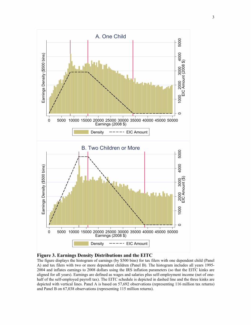
Figure 3 reports the histograms for earnings of tax filers with one child dependent (Panel A)

and two or more children dependents (Panel B) by bins of $500. All histograms are presented

using population weights. The graphs also depict the corresponding EITC schedules (as a

function of earnings) in dashed lines using the right y-axis as well as the location of the kinks

in vertical lines. To obtain a large sample size and hence smoother histograms, the figure

combines all years from 1995 to 2004 and indexes earnings to 2008 using the IRS inflation

parameters so that the EITC kinks are perfectly aligned for all years.

Two elements are worth noting on Figure 3. First, there is a clear clustering of tax filers

around the first kink point of the EITC. In both panels, the density is maximum exactly at11Since 1994, tax filers with no children are also eligible to a modest EITC (maximum benefit of $438 in

2008) with small phase-in and phase-out rates of 7.65 percent. Because the EITC with no children is so small,we do not include it in our analysis.

10

the first kink point. The fact that the location of the first kink point differs between EITC

recipients with one child versus those with two or more children constitutes strong evidence

that the clustering is driven by behavioral responses to the EITC as predicted by the standard

model. Second, however, we cannot discern any systematic clustering around the second kink

point of the EITC. Similarly, we cannot discern any gap in the distribution of earnings around

the concave kink point where the EITC is completely phased-out. This differential response

to the first kink point versus the other kink points is surprising in light of the standard

model which predicts that any convex (concave) kink should produce bunching (gap) in the

distribution of earnings.

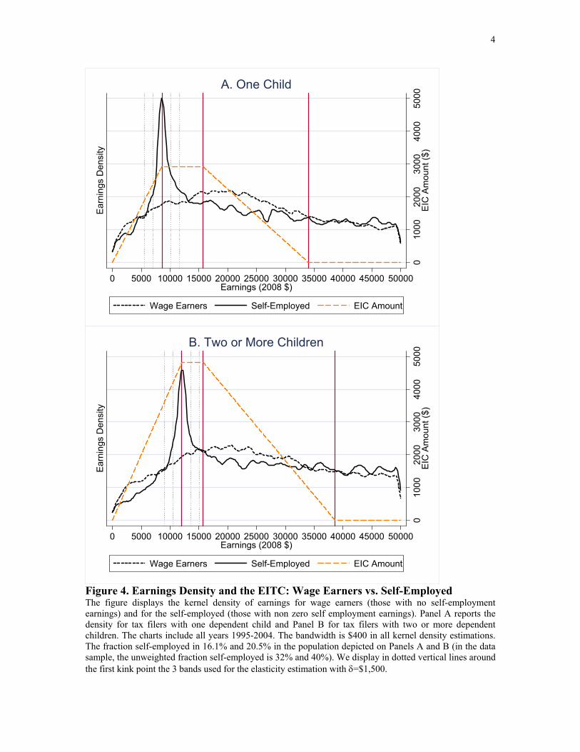
In Figure 4, we break down the sample of earners into those with non-zero self-employment

income versus those zero self-employment income (and hence whose earnings comes only from

wages and salaries). We now report kernel density estimates (instead of histograms) to compare

densities on the same graph.12 The densities are normalized to sum to one.13 The contrast

between the two groups is striking. The self-employed densities display a huge spike exactly

at the first kink point while there is no evidence of bunching at all in the sample of pure wage

earners. There is no evidence of bunching at the second kink point or of a dip at the end of

the phase-out, even for the self-employed sample. Surprisingly, note that the self-employed

with one qualifying child display even more bunching that those with two or more qualifying

children, even though the size of the kink is larger for the former group.14

Figure 5 focuses on the self-employed and breaks down the sample into two periods 1995-

1999 (dashed line density) and 2000-2004 (solid line density). The graphs show that bunching

grows dramatically from 1995-1999 to 2000-2004. The most plausible explanation is that

information and knowledge on how to game the EITC with self-employment income diffuses

slowly in the population. An alternative explanation could be that there are large adjustment

costs to changing labor supply (such as finding a new job, adjusting hours of work, etc.) which

create a slow dynamic response to the EITC expansion. The information explanation seems12The artificial drop in the kernel densities at each end of the graph is an artifact of the estimation method

due to data truncation.13The fraction of self-employed in the population depicted on Figure 4 is 16.1 percent (for those with one child

in Panel A) and 20.2 percent (for those with two or more children in Panel B) on average for years 1995-2004.In the data sample, the fractions self-employed are higher (32 percent and 40 percent respectively) because thedata samples overweight tax filers with more complex tax returns.

14This pattern of bunching is similar across heads of household and married tax filers. There is never bunchingamong wage earners while there is sharp bunching among the self-employed but only at the first kink point.

11

more plausible because bunching growth is present only among the self-employed and never

happens for wage earners (figures omitted, see elasticity estimates below).

2.2 Elasticity Estimation

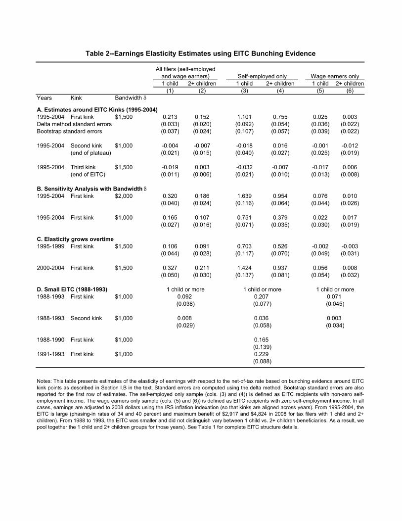
Table 2 presents elasticity estimates using bunching evidence around EITC kink points for

various samples. The table is organized in 6 columns. The first two columns are for the full

sample including both wage earners and the self-employed. The next two columns consider

the self-employed (defined as above as those with non-zero self-employment income). The last

two columns consider the sample of wage earners (those with no self-employment income). In

each of those three groups, the first column is for tax filers with one child while the second

column is for tax filers with two or more children.

Panel A displays the elasticity estimates for the first, second, and third kink points (re-

spectively) pooling all years 1995-2004 together as on Figures 3 and 4. Our results confirm the

findings from the figures. We find significant elasticities around the first kink point for the full

sample (0.21 and 0.15 for 1 child and 2+ children respectively). Those significant elasticities

are driven entirely by the self-employed who display very large and precisely estimated elas-

ticities (1.1 and 0.8 for 1 child and 2+ children respectively). In contrast, we find insignificant

elasticities very close to zero and precisely estimated for the sample of wage earners around

the first kink point. We also find insignificant and precisely estimated elasticities around the

second and third kink points in all samples (all workers, the self-employed, or wage earners).

Panel B shows the sensitivity of our results with respect to the choice of the bandwidth

δ around the first kink point.15 The bands corresponding to the baseline δ = $1, 500 were

depicted on Figure 4 (light dotted vertical lines). They represent a conservative choice of

bandwidth leading to an underestimate of the elasticities as Figure 4 shows that the lower and

upper bands densities are already affected by the clustering around the kink. Therefore, it is

not surprising that increasing the bandwidth to $2,000 leads to even higher estimates, which

we view as probably closer to the true elasticity revealed by bunching behavior. Conversely,

lowering the bandwidth to $1,000 leads to smaller (but still significant) estimates.16 This15The estimates around the second and third kink points are always small and insignificant and not sensitive

to δ, and hence omitted to save space.16It is possible to test for equality of estimated elasticities across various bandwidth specifications by esti-

mating the difference in elasticities simultaneously and using again the delta method. Differences in elasticitiesbetween δ = $1000 and δ = $2000 are indeed always significant for the first four 4 rows.

12

confirms that, in the presence of clustering around a kink point instead of exact bunching, the

choice of the bandwidth matters. In this paper, we use a simple graphical visual approach

for selecting the bandwidth which is a significant limitation. As mentioned above, with larger

datasets and hence smoother density estimates, it could be possible to devise a method to

detect bunching humps statistically and hence choose the bandwidth δ with a systematic

econometric method.

Panel C breaks the sample into two periods 1995-1999 versus 2000-2004 as we did in

Figure 5. The results confirm the graphical evidence and show that the elasticities more than

double from the early period to the late period (again the difference in elasticities across the

two periods is significant in the first 4 columns, formal test results omitted). However, the

elasticities for wage earners remain close to zero and insignificant even in the late period,

suggesting that labor supply is unresponsive along the intensive margin even in the long run.

Finally, Panel D presents results for the smaller EITC for the period 1988-1993 when the

phase-in subsidy rate was much smaller as reported in Table 1, (14 percent from 1988-1990

and growing slowly to almost 20 percent from 1991 to 1993). The elasticity estimates are

also significant for the first kink point and close to 0.3 for the self-employed. Those elasticity

estimates are much lower than for the large EITC period. There is interesting heterogeneity

during this “small EITC” period: the elasticity estimate for the self-employed is not significant

for the early period 1988-1990 when the EITC rate was 14 percent while it becomes significant

during the years 1991, 1992, 1993 when the EITC rate is 17 percent, 18 percent, and 19 percent

(on average). Graphical evidence (omitted for sake of space) shows indeed that there is no

sharp spike at the kink point in 1988-1990 but that a spike develops exactly at the kink point

in years 1991-1993.17

2.3 Interpretation: A Model of Tax Reporting

Our first finding is that wage earners do not display any evidence of responses to the marginal

incentives created by the EITC even when the change in marginal incentives is very large and

the EITC schedule is stable (as is the case since 1995). There are several possible explanations.17Using one single annual cross section of the same tax data we have used in this study, Jeffrey Liebman (1998)

did not find evidence of bunching at the EITC kink points in 1992 (before the large EITC expansion). However,he did not break down recipients by self-employment status, explaining why, in contrast to our findings, he didnot uncover evidence of bunching.

13

First, wage earners may have a very low intensive elasticity of earnings with respect to marginal

tax rates. Second, wage earners may not understand the marginal incentives created by the

EITC.18 Third, low income wage earners may not have the flexibility to adjust their labor

supply (as employers may impose hours constraints) or may not be able to control their

earnings accurately (as work opportunities may be highly stochastic). Finally, wage earners

may not be able to misreport their earnings to take advantage of the EITC because wage

income is third-party reported by employers making tax evasion difficult.

Our second finding is that the self-employed display significant bunching evidence. Consis-

tent with the standard model, the self-employed are likely to be more responsive to marginal

incentives because they may have more flexibility to adjust their labor supply or can misreport

their income with less risk of being caught evading.19 As shown by Feldstein (1999), such tax

avoidance behavior can be easily be modelled using the standard two good utility framework

introduced in Section I as long as the costs of evasion are convex with the level of evasion.

However, our bunching evidence among the self-employed remains inconsistent with the stan-

dard model in two important ways. First, bunching is found only at the first kink point and

not at the second kink point (nor is there evidence of a gap in the earnings density at the third

concave kink point). Second, even at the first kink point, bunching arises only when the EITC

subsidy rate is over 15 percent: bunching evidence starts in 1991 when the EITC subsidy rate

is above 16 percent, and becomes very large with the modern EITC with subsidy rates of 34

percent and 40 percent.20

Self-employment income reported on individual tax returns also faces the Social Security

and Medicare payroll tax at a rate of 15.3 percent.21 For the self-employed, the payroll tax is

administered with the individual income tax return. Therefore, the first kink of the EITC is the

point that maximizes the net transfer received from the government when the EITC subsidy18Lack of knowledge about the structure of the EITC is indeed confirmed by surveys of low and moderate

income families (see e.g., Lynn M. Olson and Audrey Davis 1994, Jennifer L. Romich and Thomas S. Weisner2002).

19Indeed, in the case of small informal business suppliers, the IRS estimates that the rate of income under-reporting is extremely high–over 80 percent for tax year 1992 (U.S. Treasury, Internal Revenue Service, 1996,Table 3, p. 8).

20We have also verified that no bunching develops with the EITC for filers with no children with a subsidyrate of 7.65 percent.

21In reality, the effective rate is slightly lower as the payroll tax applies to a base of 92.35 percent of self-employment income (to be equivalent to the sum of employer and employee payroll taxes in the case of wageearnings). However, the EITC is also based on 92.35 percent of self-employment income. Hence, the rate of15.3 percent is the relevant number to compare to the nominal EITC subsidy rate.

14

rate is over 15.3 percent.22 Many low income earners do have some informal self-employment

income because they perform informal services for pay such as child care, cleaning, landscaping,

house or car maintenance, etc. This informal income cannot be monitored by the IRS and is

therefore in general not reported on tax returns (which explains the extremely large 80 percent

evasion rate for informal supplier business income mentioned above). However, with an EITC

subsidy rate above the payroll tax rate, it is to the advantage of low income earners to report

such informal self-employment income. As the IRS cannot monitor the amounts, it is also

possible to over-report such informal self-employed income.23

The following simple model of behavior can account for the facts we have uncovered in our

empirical analysis of bunching around EITC kink points. Each individual has formal earnings

w ≥ 0 (wages and salaries or formal self-employment income reported to the IRS on third

party W2 or 1099 forms) and informal earnings y ≥ 0 (self-employment income not reported

on third party 1099 forms). Let us assume that both w and y do not respond to taxes along the

intensive margin (responses along the extensive margin would not affect the analysis and are

ignored) and are smoothly distributed in the population. Individuals cannot misreport formal

earnings w but can misreport y. Let us denote y the amount of informal earnings reported

for tax purposes. Taxes and transfers are based on w + y so that net disposable income is

c = w + y − T (w + y).

The critical element to obtain bunching solely at the first kink point global maximum and

not at the other kink points, as we observed in our empirical analysis, is to assume away convex

preferences and instead use linear preferences with fixed costs. Let us therefore assume that

there is an administrative fixed cost qA to report y > 0 which represents record keeping, filing

additional tax schedules, as well as determining the corresponding tax liability. We further

impose the constraint that y ≥ 0 by assuming that y < 0 would trigger an audit. As mentioned

above, EITC bunching is not generated by those reporting negative self-employment income.

There is also a moral fixed cost qM of misreporting y that is paid whenever y 6= y. This

latter cost can be a moral cost of cheating the government or can represent the risk of being22The EITC first kink point remains the income level maximizing the net transfer received from the govern-

ment even after the introduction of the refundable child tax credit in 2001.23Interestingly, we find that the spike around the first kink point is entirely due to tax filers reporting positive

self-employment income and not at all to tax filers reporting negative self-employment income, suggesting thattax filers in the phasing-out range do not avoid taxes by reporting exaggerated business losses. An explanationcould be that net business losses are much more likely to trigger an IRS audit than business gains.

15

audited and caught misreporting income by the IRS. Importantly, the fixed cost qM is paid

whenever some evasion happens.24 It could be possible to add, on top of the fixed cost qM ,

a variable cost depending linearly on the amount of tax evasion without affecting the nature

of the results. We omit such a variable cost to simplify the presentation.25 We assume for

simplicity (and without affecting the analysis) that utility is quasi-linear in disposable income

c. Therefore, an individual chooses y to maximize:

w + y − T (w + y)− qA · 1(y > 0)− qM · 1(y 6= y). (7)

Let us assume that −T (z) is single peaked and that z∗ is the unique reported income which

maximizes the government net transfer −T (z). The US federal, state, and payroll tax system

does generate such single peaked transfers. If the EITC subsidy rate is above the payroll tax

rate, then z∗ is at the first kink point of the EITC and otherwise, z∗ = 0. Let us assume

further that the distribution of costs (qA, qM ) is smooth in the population. We can state the

following formal proposition.

Proposition 1 In our reporting model with non-convex preferences, we have

(a) The optimal report for self-reported income y can take only three values: (1) truthful

reporting y = y, (2) complete evasion y = 0, or (3) maximizing the tax refund y = z∗ − w.

(b) If z∗ > 0 (i.e., the EITC subsidy rate is larger than the payroll tax rate), then an atom

of tax filers will bunch at the first kink point of the EITC z∗.

Proof: For (a), consider first the case where z∗ − w ≥ 0 and suppose that y > 0 and y 6= y,

then y delivers at least as much utility as reporting z∗ − w, hence −T (w + y) ≥ −T (z∗). As

z∗ uniquely maximizes −T (z), it must be the case that w + y = z∗. Hence if z∗ − w ≥ 0, we

are necessarily in scenario (1), (2), or (3).

Second, consider the case z∗ − w < 0 where the first kink point is not reachable with any

y ≥ 0. Because −T (z) is single peaked, y = 0 maximizes −T (w+ y). Therefore, if y 6= y, then

y = 0 is the optimal choice. So, we are necessarily in scenario (1) or (2).24If the IRS can demonstrate that self-employment income was misreported (which is actually difficult in the

case of informal business income), then the tax filer has to pay the evaded tax. As fines are rarely imposed inthe case of small amounts, there is little monetary cost to cheating. Therefore, the fixed cost represents thepsychological cost of going through the process of being audited by the IRS. Janet McCubbin (2000) reportsthat, although less than 20 percent of EITC report self-employment income, 50 percent of audited EITC returnswhich have income errors reported some self-employment income.

25A convex cost of evasion as in the conventional tax evasion model would bring back convex preferences,and would generate bunching at the second kink point of the EITC, at odds with our empirical findings.

16

For (b), from (7), the tax filer chooses scenario (1), (2), or (3) depending on which of the

three expressions, (1) w + y − T (w + y)− qA · 1(y > 0), (2) w + y − T (w)− qM · 1(y 6= 0), (3)

w + y − T (z∗)− qA · 1(z∗ − w > 0)− qM · 1(y 6= z∗ − w), is largest.

Assuming that z∗ > 0, then all filers such that qM < T (w + y)− T (z∗) and qA < T (w)−

T (z∗) will bunch at the kink. Because z∗ is the single global maximum of −T (z), we have

T (w + y) − T (z∗) > 0 and T (w) − T (z∗) > 0 for w 6= z∗ and w + y 6= z∗. Therefore, as qM

and qA are smoothly distributed, there is a positive measure of tax filers bunching at the kink

point z∗.

Three points are worth noting. First, if the EITC subsidy rate is smaller than the payroll

tax rate, then z∗ = 0. Tax filers are either truthful or do not report informal earnings at all and

there is no bunching at the first kink of the EITC. This represents the standard case described

in Tax Compliance studies where most informal self-employment earners do not report their

self-employment income.

Second, when the EITC subsidy rate becomes larger than the payroll tax rate, then bunch-

ing develops at the first kink point of the EITC. Bunching tax filers are tax filers who previously

did not report at all their self-employment income (for whom the gain of maximizing the net

credit is larger than the administrative cost qA) or tax filers who were previously truthful (for

whom the gain of maximizing the net credit is larger than the moral cost qM ). Consistent

with the evidence, there will be no bunching at the second kink point because that point does

not maximize the net tax credit.

Third, the amount of bunching depends positively on the size of the net-tax credit −T (z∗).

The increased bunching that we observed overtime on Figure 5 could be modelled as a learning

process whereby Tax filers learn slowly overtime from others or from tax preparers that report-

ing z∗ maximizes net tax transfers. Importantly, increasing the EITC at the margin generates

deadweight burden in our model because tax filers who change their behavior because of the

(marginal) EITC change generate a first order fiscal cost but experience a second order welfare

gain. Therefore, as in the standard model, the indirect fiscal costs due to behavioral reporting

responses are deadweight burden. The size of the marginal deadweight burden is proportional

to the size of the behavioral response.

17

3 Federal Income Tax Empirical Results

Last, we turn to the analysis of bunching around the kinks of the regular federal income tax

schedule. We first provide background on federal income tax computation, and then turn to

the empirical analysis. In contrast to our previous EITC analysis, the results for the regular

federal income tax are not as striking and it does not seem possible to provide a simple

theoretical model accounting for all the empirical facts, explaining why we discuss the regular

federal income tax in this separate section.

3.1 Background on Federal Income Tax Computation

For federal income tax purposes, taxable income is defined as Adjusted Gross Income (AGI) less

personal exemptions (a fixed amount per person in the tax unit) and deductions. Deductions

can take the form of a standard deduction (a fixed amount depending on marital status:

single, married, or head of household) or of itemized deductions whichever is larger. Itemized

deductions include state and local income and property taxes, mortgage interest payments,

charitable contributions, and other smaller items. Income tax is computed as a function of

taxable income using a piece-wise linear schedule with increasing marginal tax rates.26 The

size of the tax brackets depends on marital status. The relevant income measure to study

bunching around the kinks of the regular federal income tax schedule is therefore taxable

income.

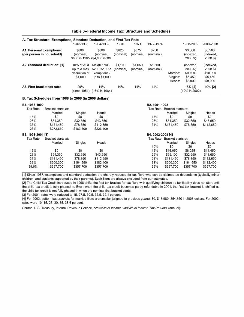
Before the Tax Reform Act (TRA) of 1986, there was a large number of tax brackets

(between 15 and 25 depending on years) and thus jumps in marginal tax rates from bracket to

bracket were small–from 1 to 5 percentage points in general, except for the first bracket where

tax liability begins. As shown on Table 3, Panel A, the first bracket had a tax rate between

14 percent and 20 percent depending on years. Moreover, before TRA 1986, the tax schedule

was not indexed for inflation, and thus the real location of kinks changed substantially from

year to year during the inflationary episodes of the 1970s–a phenomenon called ‘bracket creep’.

The exemption and standard deduction amounts were also adjusted periodically to mitigate

‘bracket creep’. Thus, we limit our study of bunching in the pre-TRA era primarily to years

1960 to 1969, when inflation was low and the tax schedule stable, and only to the vicinity of26There are a number of exceptions to that rule, such as favorable treatment of realized capital gains or the

alternative minimum tax.

18

the first kink point.27 As described in Panel A of Table 1, the income tax structure has been

remarkably stable from 1948 to 1963, with the exemption level per person fixed at $600 (in

nominal dollars), and the standard deduction defined as 10 percent of AGI (up to a maximum

standard deduction limit of $1,000) and the first marginal tax rate equal to 20 percent. In

1964, a more advantageous standard deduction equal to $200 plus $100 times the number

of exemptions was introduced. Finally, due to inflationary pressures, the modern standard

deduction was introduced in 1970 and the exemption levels increased.

After TRA 1986, the number of tax brackets was drastically reduced and exemptions,

standard deductions, tax and EITC brackets have all been indexed to the Consumer Price

Index. Table 3 (Panel B) describes the tax schedule for years 1988 to 2008 (expressed in 2008

dollars). The tax structure has changed relatively little from 1988 to 2001, and includes two

major kinks: the first kink where the marginal tax rate jumps from 0 to 15 percent, and the

second kink with a jump from 15 to 28 percent. Note that two extra tax brackets have been

introduced in 1993, creating jumps from 31 to 36 percent and 36 percent to 39.6 percent for

high income earners. In 2002, a bottom bracket with a lower rate of 10 percent was introduced

so that the jump in marginal tax rate at the first kink point is from 0 percent to 10 percent.

Furthermore, the upper rates has also been reduced from 2001 to 2003.

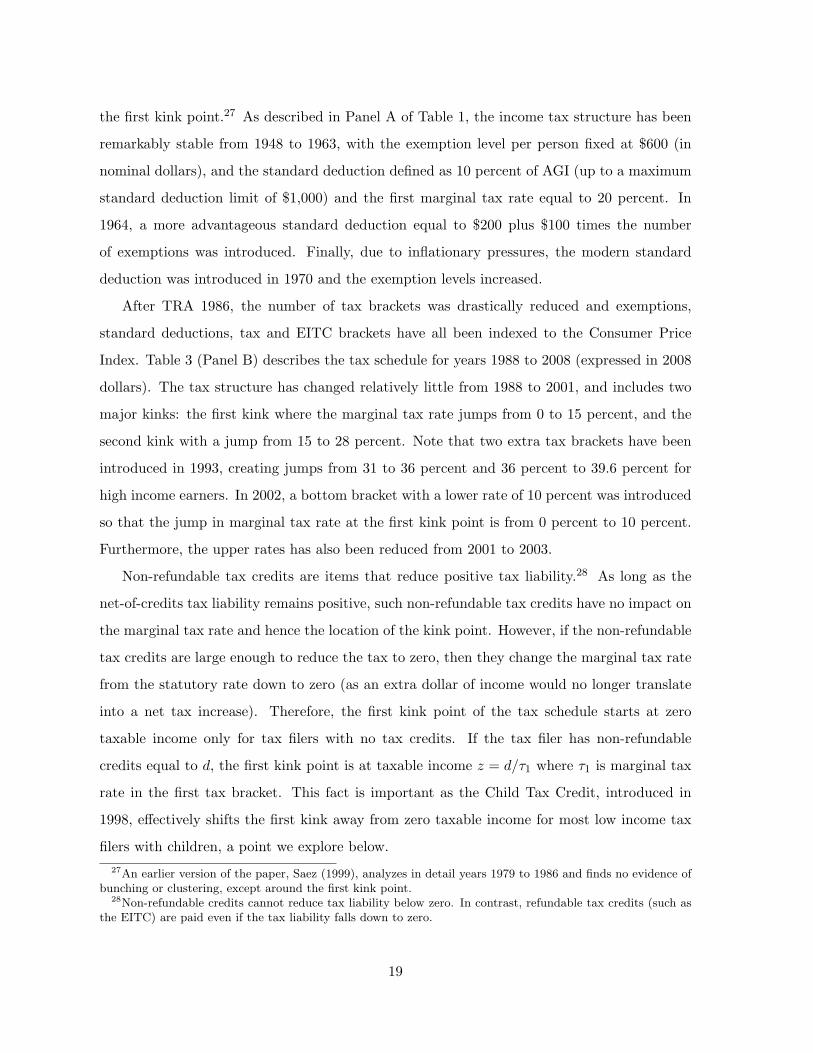
Non-refundable tax credits are items that reduce positive tax liability.28 As long as the

net-of-credits tax liability remains positive, such non-refundable tax credits have no impact on

the marginal tax rate and hence the location of the kink point. However, if the non-refundable

tax credits are large enough to reduce the tax to zero, then they change the marginal tax rate

from the statutory rate down to zero (as an extra dollar of income would no longer translate

into a net tax increase). Therefore, the first kink point of the tax schedule starts at zero

taxable income only for tax filers with no tax credits. If the tax filer has non-refundable

credits equal to d, the first kink point is at taxable income z = d/τ1 where τ1 is marginal tax

rate in the first tax bracket. This fact is important as the Child Tax Credit, introduced in

1998, effectively shifts the first kink away from zero taxable income for most low income tax

filers with children, a point we explore below.27An earlier version of the paper, Saez (1999), analyzes in detail years 1979 to 1986 and finds no evidence of

bunching or clustering, except around the first kink point.28Non-refundable credits cannot reduce tax liability below zero. In contrast, refundable tax credits (such as

the EITC) are paid even if the tax liability falls down to zero.

19

3.2 Bunching Evidence around the First Kink Point from 1960-1972

Figure 6 displays the density distributions of taxable income, expressed in 2008 dollars and

aggregating years 1960 to 196929 for married joint filers (Panel A), and singles and heads of

household (Panel B). The marginal tax rate schedules are also displayed (for year 1960) in

dashed line. In all years, the first kink point is at zero as depicted by the vertical line. Both

panels display visual evidence of bunching at the first kink point of the tax schedule although

bunching is less pronounced in Panel B. In both cases, the density peaks just before the

first kink point, providing compelling evidence that the change in marginal tax rates around

the first kink point produces a behavioral response of reported taxable income. A potential

objection is that individuals may not systematically file tax returns in the negative range of

taxable income as no tax liability is due. Figure 6, however, shows that there is no missing

density just below the kink as the density is actually higher just below the kink. Indeed, in

practice, withholding on wage income starts below the zero taxable income threshold so that

most filers with low wage income and negative taxable income file to obtain a tax refund.

Figure 7 casts further light on the mechanism behind the bunching uncovered on Figure

6 by plotting the kernel density of taxable income (as in Figure 6) along with the density

of taxable income computed using the standard deduction, i.e., defined as adjusted gross

income minus personal exemptions and minus the standard deduction (even for itemizers).

The graphs show that bunching is much more pronounced for actual taxable income than for

taxable income computed with the standard deduction, especially in the case of married filers

(Panel A). This shows that the bunching phenomenon is in large part due to the response

of itemized deductions. We expect indeed itemizers to be able to bunch exactly at the spike

because some of the itemized deductions such as charitable contributions might be manipulated

much more easily than earnings. For example, some taxpayers who itemize deductions might

bunch exactly at the kink because they may stop reporting deductions once they have reached

the threshold of no tax liability. Note however, that even taxable income computed with the

standard deduction displays some bunching around the first kink point, especially for single

filers, suggesting that part of the response is an adjusted gross income response.

Figure 8 casts light on the dynamics of bunching by showing taxable income densities for29Years 1961, 1963, and 1965 are not included because no micro file was created for these years.

20

three periods: 1960-1963, 1964-1969, and 1970-1972. As discussed above, from 1954 to 1963,

the tax system around the first kink point was totally stable in nominal terms and inflation

was low. In 1964-65, the standard deduction was expanded and the first tax rate lowered from

20 to 14 percent. Finally, in 1970-72, because of high inflation and the concern of ‘bracket

creep’, both the personal exemptions and standard deductions were further expanded from

year to year. Figure 8 shows that tax filers are not able to adapt immediately to the changes

in the tax system and that bunching is less pronounced in the last two periods and especially

in 1970-72 when the tax system changes every year. Note that the bunching reduction is even

more pronounced for single filers possibly because bunching for singles is primarily due to

income responses instead of itemized deduction responses as shown in Figure 7. Overall, those

results are consistent with our previous EITC evidence suggesting that it takes time for filers

to learn and adjust to the tax system.

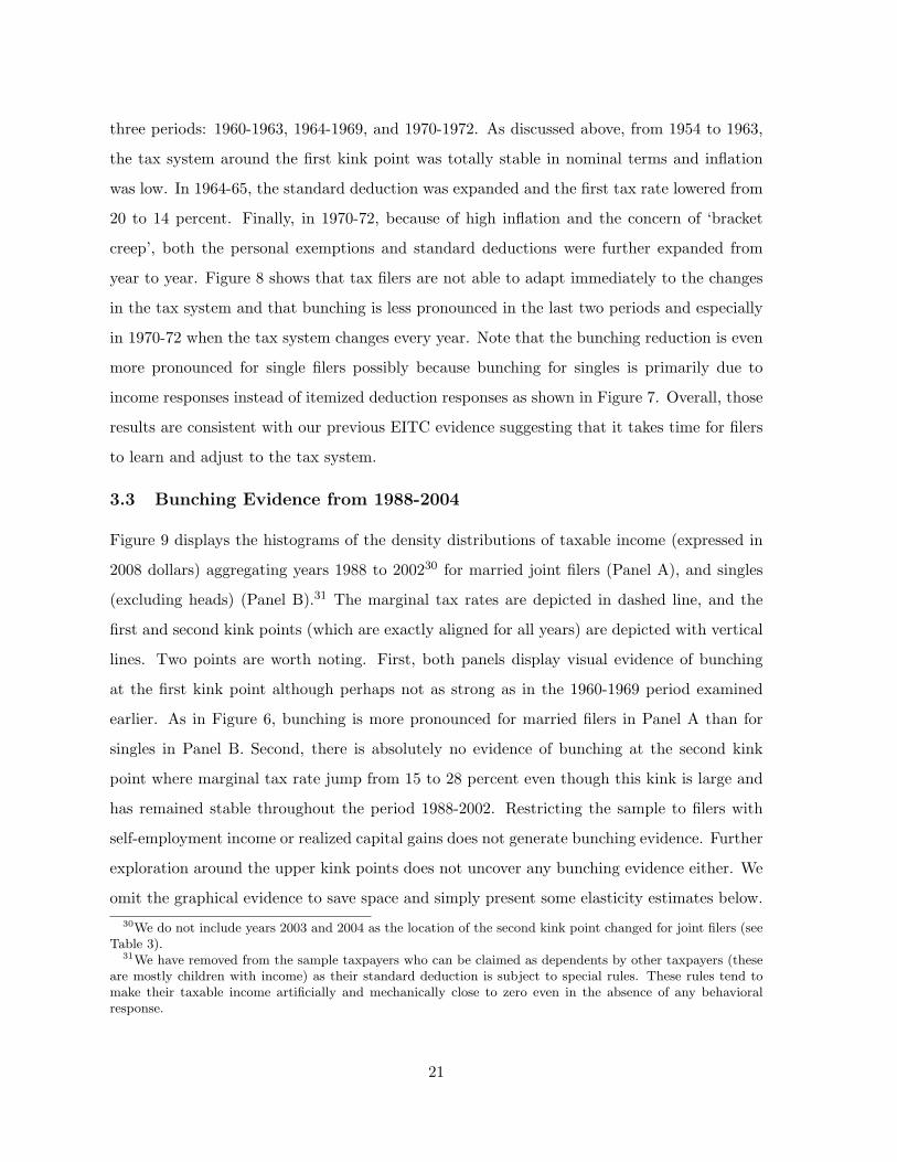
3.3 Bunching Evidence from 1988-2004

Figure 9 displays the histograms of the density distributions of taxable income (expressed in

2008 dollars) aggregating years 1988 to 200230 for married joint filers (Panel A), and singles

(excluding heads) (Panel B).31 The marginal tax rates are depicted in dashed line, and the

first and second kink points (which are exactly aligned for all years) are depicted with vertical

lines. Two points are worth noting. First, both panels display visual evidence of bunching

at the first kink point although perhaps not as strong as in the 1960-1969 period examined

earlier. As in Figure 6, bunching is more pronounced for married filers in Panel A than for

singles in Panel B. Second, there is absolutely no evidence of bunching at the second kink

point where marginal tax rate jump from 15 to 28 percent even though this kink is large and

has remained stable throughout the period 1988-2002. Restricting the sample to filers with

self-employment income or realized capital gains does not generate bunching evidence. Further

exploration around the upper kink points does not uncover any bunching evidence either. We

omit the graphical evidence to save space and simply present some elasticity estimates below.30We do not include years 2003 and 2004 as the location of the second kink point changed for joint filers (see

Table 3).31We have removed from the sample taxpayers who can be claimed as dependents by other taxpayers (these

are mostly children with income) as their standard deduction is subject to special rules. These rules tend tomake their taxable income artificially and mechanically close to zero even in the absence of any behavioralresponse.

21

Figure 10 provides additional evidence on bunching around the first kink point. Panel

A displays the kernel density for taxable income and taxable income computed using the

standard deduction (as in Figure 7). The sample includes all filers married, singles, and

heads. Consistent with the period 1960-1969, bunching is much less sharp for taxable income

computed using the standard deduction but does not disappear entirely showing that part of

the response is an income response and part of the response goes through itemized deductions.

Using the introduction and development of the child tax credit in 1998, Panel B shows

further evidence that the bunching at zero taxable income is indeed created by the jump in

marginal tax rate. As mentioned above, with non-refundable credits, the first kink in the

budget set is actually not at zero taxable income but at z = d/τ1 where τ1 is marginal tax rate

in the first tax bracket and d is the amount of potential tax credits. Virtually all filers with

low taxable income and children qualify for the (non-refundable) child tax credit introduced in

1998 (as the refundable portion is not large enough to eliminate tax liability entirely in most

cases, see footnotes in Table 3). Therefore, after 1998, tax filers with children do not face a

kink at zero taxable income and hence should not bunch at zero. Figure 10, Panel B, displays

the density for tax filers with children and tax filers without children for the period 1998-2004

and shows indeed that bunching disappears for tax filers with children during the period.

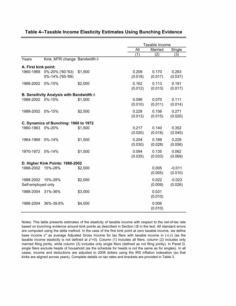
3.4 Elasticity Estimates

Table 4 provides elasticity estimates based on the graphs displayed earlier and confirms our vi-

sual evidence. Four points are worth noting. First, Panel A shows that the elasticity estimates

are consistently positive and significant and around 0.2 around the first kink point both for

the 1960-1969 period and the recent 1988-2002 period. Second, Panel B shows that estimates

are somewhat sensitive to the choice of the bandwidth δ in the estimation. As in the case of

our EITC based estimates, large bandwidth generate larger elasticities as the excess bunching

will be larger. Note that even with lower bandwidth, the estimates remain significant. Third,

Panel C shows that estimates are largest for the 1960-1963 period and are reduced significantly

by 1970-1972 especially for single filers confirming our finding that it takes time for tax filers

to adapt to a new tax schedule. Fourth, Panel D shows that estimated elasticities are zero

and precisely estimated around the higher kink points in the recent period, even when the

sample is restricted to those with positive self-employment income. Our bunching evidence for

22

higher kink points is not consistent with the standard model of static labor supply presented

in Section I.A which underpins most recent studies on the elasticity of taxable income with

respect to net-of-tax rate (see Saez, Joel Slemrod, and Seth Giertz 2009 for a recent survey)

if taxable income elasticities are substantial. It is possible that upper income tax filers have

income realizations that are partly stochastic preventing them from bunching exactly at the

kink. As we mentioned in Section I.A, it is also conceivable that for higher income earners,

labor supply is in large part driven by dynamic considerations (such as trying to obtain a

promotion), in which case the local Frisch elasticity is small and hence bunching is also small.

4 Conclusion

Our analysis has found substantial evidence of bunching around the first kink point of the EITC

but concentrated among those reporting self-employment income. For the federal income tax,

we have found evidence of bunching only at the first kink point where tax liability starts

with no evidence of bunching for higher kink points. We have also developed an econometric

method which uses bunching evidence to estimate the intensive elasticity of reported income

with respect to (one minus) the marginal tax rate in the standard micro-economic model.

Several of our empirical findings suggest that the standard intensive labor supply model

cannot fully account for the facts. In the case of the EITC, we have shown that all our empirical

findings can be much better explained by a fully rational fixed cost model of misreporting

informal self-employment income. In contrast to the standard model, this alternative model

can successfully explain why we observe bunching solely for the self-employed and solely around

the first EITC kink point (and not around the other EITC kink points) and only when the

EITC subsidy rate is larger than the payroll social security tax.

The contrasting evidence of bunching around the first kink point of the federal income

tax with no bunching evidence at all around higher kink points also appears inconsistent with

the standard static model presented in Section I.A. Possible explanations consistent with our

empirical evidence include (a) larger elasticities at the bottom than in the middle or upper

part of the income distribution, (b) more flexibility in hours choice and earnings decisions at

the bottom, (c) the difficulty for tax filers to understand the exact details of a complex tax

system as the first kink point where tax liability starts is likely to be more salient and easier

23

to understand than other kink points.

The elasticity estimation framework proposed here could be applied to other contexts where

nonlinear budget sets create convex kink points and where individuals are likely to be aware

of those kinks. Examples include (1) the Social Security earnings test where previous work

(Burtless and Moffitt 1984, Friedberg, 2000) has found evidence of bunching consistent with the

standard model, (2) 401(k) pension contributions where employers often provide a match up

only up to some level of contributions and where numerous studies have documented evidence of

bunching of contributions where the cap ends (see e.g., James Choi et al. 2002), (3) retirement

decisions as public and private defined benefits retirement systems often introduce kinks in the

lifetime budget constraint,32 (4) household consumption of utilities (such as telephone, water,

gas, and electricity) where pricing is often piecewise linear.33, (5) tax systems in other countries

which sometimes offer larger and more transparent kink points than the US system. Chetty et

al. (2009) have just proposed such an analysis for Denmark. In all of those cases, it would be

particularly valuable to analyze whether providing information about the nonlinearities could

affect behavior.34

32As mentioned in introduction, Brown (2007) proposed a bunching based elasticity estimation using reformsin the California Teachers retirement program.

33Severin Borenstein (2008) analyzes the case of nonlinear electricity pricing in California and finds no evidenceof bunching.

34Chetty and Saez (2009) show that information about the EITC does increase the amount of bunchingaround the first kink point of the EITC.

24

References

Blundell, Richard, and Hilary Hoynes. 2004. “Has In-Work Benefit Reform Helped theLabour Market?” In Seeking a Premier Economy: The Economic Effects of British EconomicReforms, 1980-2000, ed. David Card, Richard Blundell and Richard Freeman. University ofChicago Press: Chicago.Borenstein, Severin. 2008. “Equity (and some efficiency) Effects of Increasing-Block Elec-tricity Pricing.” UC Berkeley Working Paper.Brown, Kristine M. 2007. “The Link between Pensions and Retirement Timing: Lessonsfrom California Teachers.” PhD diss. University of California, Berkeley.Burtless, Gary, and Jerry Hausman. 1978. “The Effect of Taxation on Labor Supply:Evaluating the Gary Income Maintenance Experiment.” Journal of Political Economy 86:1103-1130.Burtless, Gary, and Robert Moffitt. 1984. “The Effect of Social Security Benefits on theLabor Supply of the Aged.” In Retirement and Economic Behavior, ed. Henry Aaron andGary Burtless. Washington: Brookings Institution.Chetty, Raj, John N. Friedman, Tore Olsen, and Luigi Pistaferri. 2009. “The Effectof Adjustment Costs and Institutional Constraints on Labor Supply Elasticities: Evidencefrom Denmark.” UC Berkeley mimeo July.Chetty, Raj and Emmanuel Saez. 2009. “Teaching the Tax Code: Earnings Responsesto an Experiment with EITC Claimants.” NBER Working Paper No. 14836.Choi, James J., David Laibson, Brigitte Madrian, and Andrew Metrick. 2002.“Defined Contribution Pensions: Plan Rules, Participant Decisions, and the Path of LeastResistance.” In Tax Policy and the Economy, ed. James Poterba, 16, 67-114. Cambridge MA:MIT Press.Eissa, Nada and Hilary Hoynes. 2006. “Behavioral Responses to Taxes: Lessons from theEITC and Labor Supply.” In Tax Policy and the Economy, ed. James Poterba, 20, 74-110.Cambridge MA: MIT Press.Feldstein, Martin. 1999. “Tax Avoidance and the Deadweight Loss of the Income Tax.”Review of Economics and Statistics, 81: 674-680.Friedberg, Leora. 2000. “The Labor Supply Effects of the Social Security Earnings Test.”Review of Economics and Statistics, 82: 48-63.Fujii, Edwin T. and Clifford B. Hawley. 1988. “On the Accuracy of Tax Perceptions.”Review of Economics and Statistics 70: 344-347.Gruber, Jonathan, and David A. Wise, ed. 1999. Social Security Programs and Retire-ment around the World. Chicago: University of Chicago Press and NBER.Hausman, Jerry. 1981. “Labor Supply.” In How Taxes Affect Economic Behavior, ed.Henry J. Aaron and Joseph A. Pechman. Washington, D.C.: Brookings Institution.

25

Hausman, Jerry. 1982. “Stochastic Problems in the Simulation of Labor Supply.” In Be-havioral Simulations in Tax Policy Analysis, ed. Martin Feldstein, 41-69. Chicago: Universityof Chicago Press.Heckman, James. 1982. “Comment.” In Behavioral Simulations in Tax Policy Analysis,ed. Martin Feldstein, 70-82. Chicago: University of Chicago Press.Hotz, V. Joseph and John Karl Scholz. 2003. “The Earned Income Tax Credit.” InMeans-Tested Transfer Programs in the United States, ed. Robert Moffitt. Chicago: Universityof Chicago Press.Lalumia, Sara. 2009. “The Earned Income Tax Credit and Reported Self-EmploymentIncome.” Williams College Working Paper.Liebman, Jeffrey. 1998. “The Impact of the Earned Income Tax Credit on Incentives andIncome Distribution.” In Tax Policy and the Economy, 12, ed. James Poterba. Cambridge:MIT Press.McCubbin, Janet. 2000. “EITC Noncompliance: The Determinants of the Misreporting ofChildren.” National Tax Journal 53(4), Part 2: 1135-1160.Moffitt, Robert. 1986. “The Econometrics of Piecewise-Linear Budget Constraints.” Jour-nal of Business and Economic Statistics, 4(3): 317-328.Moffitt, Robert. (1990) “The Econometrics of Kinked Budget Constraints.” Journal ofEconomic Perspectives, 4(2): 119-139.Olson, Lynn M. and Audrey Davis. 1994. “The Earned Income Tax Credit: Views fromthe Street Level.” Northwestern Working Paper WP-94-1.Romich, Jennifer L. and Thomas S. Weisner. 2002. “How Families View and Use theEarned Income Tax Credit: Advance Payment Versus Lump-Sum Delivery.” In Making WorkPay, ed. Bruce Meyer and Douglas Holtz-Eakin. New York: Russell Sage Foundation.Saez, Emmanuel. 1999. “Do Taxpayers Bunch at Kink Points?” NBER Working Paper No.7366, revised version June 2002 prepared for the NBER-TAPES 2002 conference.Saez, Emmanuel, Joel Slemrod, and Seth Giertz. 2009. “The Elasticity of TaxableIncome with Respect to Marginal Tax Rates: A Critical Review.” NBER Working Paper No.15012, in preparation for the Journal of Economic Literature.U.S. Treasury Department, Internal Revenue Service. Annual Statistics of Income:Individual Income Tax Returns., Publication 1304, Washington, D.C.: Government PrintingPress.U.S. Treasury Department, Internal Revenue Service (1996) Federal Tax ComplianceResearch, Individual Income Tax Gap Estimates for 1985, 1988, and 1992, Publication 1415,Washington, D.C.: Government Printing Press.

26

A. Indifference curves and bunching

After-taxincome

c=z-T(z)

Before tax income z

Slope 1-t

z* z*+dz*

Slope 1-t-dt

Individual L chooses z* before and after reformIndividual H chooses z*+dz* before and z* after reformdz*/z* = e dt/(1-t) with e compensated elasticity

Individual H indifference curves

Individual L indifference curve

B. Density Distributions and Bunching

Density distribution

Before tax income zz* z*+dz*

Before reform density

After reform density

Pre-reform incomes between z* and z*+dz* bunch at z* after reform

Figure 1. Bunching Theory Panel A displays the effect on earnings choices of introducing a (small) kink in the budget set by increasing the tax rate t by dt above income level z*. Individual L who chooses z* before the reform stays at z* after the reform. Individual H chooses z* after the reform and was choosing z*+dz* before the reform. Panel B depicts the effects of introducing the kink on the earnings density distribution. The pre-reform density is smooth around z*. After the reform, all individuals with income between z* and z*+dz* before the reform, bunch at z*, creating a spike in the density distribution. The density above z*+dz* shifts to z* (so that the resulting density and is no longer smooth at z*).

2

Density distribution

Before tax income zz*z*+δ

h(z)

z*-δz*+2δz*-2δ

h(z*)-

h(z*)+

H*-

B = H* - (H*-+ H*+ ) = excess bunching

Before reform: linear tax rate t0, density h0(z)

After reform: tax rate t0 below z*Tax rate t1 above z* (t1>t0), density h(z)

h0(z)H*+

Figure 2. Estimating Excess Bunching using Empirical Densities The figure illustrates the excess bunching estimation method using empirical densities. We assume that, under a constant linear tax with rate t0, the density of income h0(z) is smooth. A higher tax rate t1 is introduced above z*, creating a convex kink at z*. The reform will induce tax filers to cluster at z*, creating a spike in the post-reform density distribution h(z). As illustrated on the figure, bunching might not be perfectly concentrated at z* because of inability of tax filers to control or forecast their incomes perfectly or imperfect information about the exact kink location. For estimation purposes, we define three bands of income around the kink point z* using the bandwidth parameter δ. The lower band is the segment (z*-2δ,z*-δ), it has average density h(z*)- and hence includes H*-=δ h(z*)- tax filers (dashed left area). The upper band is the segment (z*+δ,z*+2δ), it has average density h(z*)+ and hence includes H*+=δ h(z*)+ tax filers (dashed right area). The middle band is the segment (z*-δ,z*+δ) and includes H* tax filers. Excess bunching is defined as B=H*-(H*-- H*+) and is the upper dashed area on the figure. If clustering of tax filers around z* is tight, excess bunching will be estimated without bias with a small δ. If clustering is not tight around z*, a small δ will underestimate the amount of excess bunching (as the lower and upper bands will include tax filers clustering around z*). However, a large δ will lead to overestimate (underestimate) excess bunching if the before reform density h0(z) is convex (concave) around z*.

3

010

0020

0030

0040

0050

00E

IC A

mou

nt (2

008

$)

Ear

ning

s D

ensi

ty ($

500

bins

)

0 5000 10000 15000 20000 25000 30000 35000 40000 45000 50000Earnings (2008 $)

Density EIC Amount

A. One Child

010

0020

0030

0040

0050

00E

IC A

mou

nt ($

)

Ear

ning

s D

ensi

ty ($

500

bins

)

0 5000 10000 15000 20000 25000 30000 35000 40000 45000 50000Earnings (2008 $)

Density EIC Amount

B. Two Children or More

Figure 3. Earnings Density Distributions and the EITC The figure displays the histogram of earnings (by $500 bins) for tax filers with one dependent child (Panel A) and tax filers with two or more dependent children (Panel B). The histogram includes all years 1995-2004 and inflates earnings to 2008 dollars using the IRS inflation parameters (so that the EITC kinks are aligned for all years). Earnings are defined as wages and salaries plus self-employment income (net of one-half of the self-employed payroll tax). The EITC schedule is depicted in dashed line and the three kinks are depicted with vertical lines. Panel A is based on 57,692 observations (representing 116 million tax returns) and Panel B on 67,038 observations (representing 115 million returns).

4

010

0020

0030

0040

0050

00E

IC A

mou

nt ($

)

Ear

ning

s D

ensi

ty

0 5000 10000 15000 20000 25000 30000 35000 40000 45000 50000Earnings (2008 $)

Wage Earners Self-Employed EIC Amount

A. One Child

010

0020

0030

0040

0050

00E

IC A

mou

nt ($

)

Ear

ning

s D

ensi

ty

0 5000 10000 15000 20000 25000 30000 35000 40000 45000 50000Earnings (2008 $)

Wage Earners Self-Employed EIC Amount

B. Two or More Children

Figure 4. Earnings Density and the EITC: Wage Earners vs. Self-Employed The figure displays the kernel density of earnings for wage earners (those with no self-employment earnings) and for the self-employed (those with non zero self employment earnings). Panel A reports the density for tax filers with one dependent child and Panel B for tax filers with two or more dependent children. The charts include all years 1995-2004. The bandwidth is $400 in all kernel density estimations. The fraction self-employed in 16.1% and 20.5% in the population depicted on Panels A and B (in the data sample, the unweighted fraction self-employed is 32% and 40%). We display in dotted vertical lines around the first kink point the 3 bands used for the elasticity estimation with δ=$1,500.

5

010

0020

0030

0040

0050

00E

IC A

mou

nt ($

)

Ear

ning

s D

ensi

ty

0 5000 10000 15000 20000 25000 30000 35000 40000 45000 50000Earnings (2008 $)

1995-1999 2000-2004 EIC Amount

A. One Child (Self-Employed only)

010

0020

0030

0040

0050

00E

IC A

mou

nt ($

)

Ear

ning

s D

ensi

ty

0 5000 10000 15000 20000 25000 30000 35000 40000 45000 50000Earnings (2008 $)

1995-1999 2000-2004 EIC Amount

B. Two or More Children (Self-Employed only)

Figure 5. Earnings Density and the EITC: Bunching Increases over Time The figure displays the kernel density of earnings for the self-employed (those with non zero self employment earnings) for 1995-1999 (dotted line) and 2000-2004 (solid line). Panel A reports the density for tax filers with one dependent child and Panel B for tax filers with two or more dependent children. The bandwidth is $600 in all estimations. The data sample sizes underlying those density estimates are 8,436 (1995-9, one child), 9883 (1995-9, 2+ children), 12,256 (2000-4, one child), 14,308 (2000-4, 2+ children). The corresponding full population sizes are 8.8, 9.9, 11.2, 12.4 million respectively.

6

0.1

.2.3

.4.5

Mar

gina

l Tax

Rat

e

Taxa

ble

Inco

me

Den

sity

-20000 -10000 0 10000 20000 30000 40000 50000 60000Taxable Income (2008 $)

Density Marginal Tax Rate

A. Married Tax Filers

0.1

.2.3

.4.5

Mar

gina

l Tax

Rat

e

Taxa

ble

Inco

me

Den

sity

-20000 -10000 0 10000 20000 30000 40000 50000 60000Taxable Income (2008 $)

Density Marginal Tax Rate

B. Single Tax Filers

Figure 6. Taxable Income Density, 1960-1969: Bunching around First Kink The figure displays the histogram of taxable income for married joint tax filers (Panel A) and single tax filers defined as all non married joint filers (Panel B). The data include years 1960, 1962, 1964, 1966-1969 (no data are available for 1961, 1963, and 1965). Histograms are based on bins $800 wide and are computed using population weights (unweighted sample sizes for Panel A and B histograms are 185,161 and 82,859 respectively). Taxable income is defined as Adjusted Gross Income minus personal exemptions minus the maximum of the standard or itemized deductions, and is expressed in 2008 dollars. The marginal tax rate schedule is displayed for 1960 in dashed line. In all years, the first kink point is at zero taxable income displayed by the vertical line on the graph (other kink points move from year to year as tax brackets are not adjusted for inflation from 1960 to 1969). The first bracket marginal tax rate is 20% from 1960-1963, 16% in 1964, and 14% in 1965-1969 (see Table 3, Panel A for complete details).

7

0.1

.2.3

.4.5

Mar

gina

l Tax

Rat

e

Taxa

ble

Inco

me

Den

sity

-20000 -10000 0 10000 20000 30000 40000 50000 60000Taxable Income (2008 $)

Taxable Income Standard Deduction MTR

A. Married Tax Filers

0.1

.2.3

.4.5

Mar

gina

l Tax

Rat

e

Taxa

ble

Inco

me

Den

sity

-20000 -10000 0 10000 20000 30000 40000 50000 60000Taxable Income (2008 $)

Taxable Income Standard Deduction MTR

A. Single Tax Filers

Figure 7. Taxable Income Density, 1960-1969: Itemizing Effects on Bunching The figure displays the kernel density of income (in 2008 dollars) for married joint tax filers (Panel A) and single tax filers (Panel B). In each panel, the solid line is the density of actual taxable income defined as in Figure 6 as Adjusted Gross Income minus personal exemptions minus the maximum of the standard or itemized deductions, while the dotted line is the density of taxable income computed solely with the standard deduction, i.e., defined as Adjusted Gross Income minus personal exemptions minus the standard deduction. Both definitions coincide for non-itemizers but differ for itemizers. This comparison reveals the contribution of itemization to bunching at the first kink point. The data include years 1960, 1962, 1964, 1966-1969. Densities are computed using population weights. Sample sizes are the same as in Figure 6. Bandwidth is $500 in all kernel density estimations.

8

Taxa

ble

Inco

me

Den

sity

-20000 -10000 0 10000 20000 30000 40000 50000 60000Taxable Income (2008 $)

1960-1963 1964-1969 1970-1972

A. Married Tax Filers

Taxa

ble

Inco

me

Den

sity

-20000 -10000 0 10000 20000 30000 40000 50000 60000Taxable Income (2008 $)

1960-1963 1964-1969 1970-1972

B. Single Tax Filers

Figure 8. Taxable Income Density, 1960-1972: Dynamics of Bunching The figure displays the kernel density of taxable income (in 2008 dollars) for married joint tax filers (Panel A) and single tax filers (Panel B) for 3 periods 1960-1963 (solid line), 1964-1969 (dashed line), and 1970-1972 (dotted line). Densities are computed using population weights. As shown in Table 3, the definition of taxable income was stable (in nominal terms) from 1948 to 1963 and was changed in 1964 and in 1970. The graphs show that bunching decreased sharply after the reforms showing that it takes time for tax filers to bunch. Sample sizes for 1960-1963, 1964-1969, 1970-1972 are 76,515, 108,646, 69,365 in Panel A and 34,636, 48,223, 21,775 in Panel B. The bandwidth is $500 in all kernel density estimations.

9

0.1

.2.3

.4.5

Mar

gina

l Tax

Rat

e

Taxa

ble

Inco

me

Den

sity

($10

00 b

ins)

-20000-10000 0 10000 20000 30000 40000 50000 60000 70000 80000Taxable Income (2008 $)

Density Marginal Tax Rate

A. Married Tax Filers

0.1

.2.3

.4.5

Mar

gina

l Tax

Rat

e

Taxa

ble

Inco

me

Den

sity

($80

0 bi

ns)

-20000 -10000 0 10000 20000 30000 40000 50000 60000Taxable Income (2008 $)

Density Marginal Tax Rate

B. Single Tax Filers

Figure 9. Taxable Income Density, 1988-2002 The figure displays the histogram of taxable income for married joint tax filers (Panel A) and single tax filers (excluding heads of households) (Panel B). The data include years 1988 to 2002. Histograms are computed using population weights (unweighted sample sizes for Panel A and B histograms are 368,173 and 239,225 respectively representing population sizes of 594 million and 587 million tax filers). Taxable income is defined as Adjusted Gross Income minus personal exemptions minus the maximum of the standard or itemized deductions, and is expressed in 2008 dollars. The marginal tax rate schedule is displayed in dashed line. Both the first and second kink points are displayed by the vertical lines on the graph and are exactly aligned in all years as the tax system is indexed for inflation (see Table 3).

10

Taxa

ble

Inco

me

Den

sity

-20000 -10000 0 10000 20000 30000 40000Taxable Income (2008 $)

Taxable Income Standard Deduction

A. Effects of Itemizing

Taxa

ble

Inco

me

Den

sity

-20000 -10000 0 10000 20000 30000 40000Taxable Income (2008 $)

children no children

B. Child Tax Credit Effects

Figure 10. Taxable Income Densities: Itemizing and Child Tax Credit Effects The figure displays the kernel density of income (in 2008 dollars). In Panel A, the solid line is the density of actual taxable income while the dashed line is the density of taxable income computed solely with the standard deduction (see Figure 7). The data include years 1988 to 2002 and all filers. The sample size is 516,859 representing 1,110 million tax filers. The bandwidth is $400 in all kernel density estimations. In Panel B, the data include years 1998 to 2004, the solid line if for filers with dependent children while the dashed line is for tax filers with no dependent children. From 1998 to 2004, the child tax credit shifts the first kink point to a positive taxable income threshold (which varies across tax filers). As a result, bunching is less pronounced at the zero taxable income threshold for tax filers with children. Sample size are 93,797 (children) and 176,411 (no children) representing 194 million and 357 million filers. Bandwidth is $500.

A. Earned Income Tax Credit Schedule from 1988-1993 (in 2008 $) [1]One or more qualifying child

EITC range Bracket Marginal Tax rate

Phase-in $0-$11,416 -14%Plateau $11,416-$18,002 0%Phase-out $18,002-$33,985 10%

B. Earned Income Tax Credit Schedule from 1995-2008 (in 2008 $) [2]One qualifying child Two or more qualifying children

EITC range Bracket Marginal Tax rate Bracket Marginal Tax rate

Phase-in $0-$8,580 -34% $0-$12,060 -40%Plateau $8,580-$15,740 0% $12,060-$15,740 0%Phase-out $15,740-$33,995 16% $15,740-$38,646 21%

Table 1--EITC Structure and Schedules

[2] In 2002-2004, EITC plateau for married filers is extended by $1,000 ($2,000 in 2005-2007, and $3,000 in 2008). In1995, phase-in and phase-out rates were 36 and 20.2 percent (instead of 40 and 21 percent) for EITC beneficiaries withtwo or more children.Source: U.S Treasury, Internal Revenue Service, Statistics of Income: Individual Income Tax Returns (annual).

In 1991: phase-in rates are 16.7 (1 child) and 17.3 percent (2+ children). Phase-out rates are 11.9 and 12.4 percent.In 1992: phase-in rates are 17.6 (1 child) and 18.4 percent (2+ children). Phase-out rates are 12.6 and 13.1 percent.In 1993: phase-in rates are 18.5 (1 child) and 19.5 percent (2+ children). Phase-out rates are 13.2 and 13.9 percent.

[1] In 1991-1993, EITC subsidy and tax rates depend on number of children (but brackets do not).

1 child 2+ children 1 child 2+ children 1 child 2+ children(1) (2) (3) (4) (5) (6)

Years Kink Bandwidth δ

A. Estimates around EITC Kinks (1995-2004)1995-2004 First kink $1,500 0.213 0.152 1.101 0.755 0.025 0.003Delta method standard errors (0.033) (0.020) (0.092) (0.054) (0.036) (0.022)Bootstrap standard errors (0.037) (0.024) (0.107) (0.057) (0.039) (0.022)

1995-2004 Second kink $1,000 -0.004 -0.007 -0.018 0.016 -0.001 -0.012(end of plateau) (0.021) (0.015) (0.040) (0.027) (0.025) (0.019)

1995-2004 Third kink $1,500 -0.019 0.003 -0.032 -0.007 -0.017 0.006(end of EITC) (0.011) (0.006) (0.021) (0.010) (0.013) (0.008)

B. Sensitivity Analysis with Bandwidth δ1995-2004 First kink $2,000 0.320 0.186 1.639 0.954 0.076 0.010

(0.040) (0.024) (0.116) (0.064) (0.044) (0.026)

1995-2004 First kink $1,000 0.165 0.107 0.751 0.379 0.022 0.017(0.027) (0.016) (0.071) (0.035) (0.030) (0.019)

C. Elasticity grows overtime1995-1999 First kink $1,500 0.106 0.091 0.703 0.526 -0.002 -0.003

(0.044) (0.028) (0.117) (0.070) (0.049) (0.031)

2000-2004 First kink $1,500 0.327 0.211 1.424 0.937 0.056 0.008(0.050) (0.030) (0.137) (0.081) (0.054) (0.032)

D. Small EITC (1988-1993)1988-1993 First kink $1,000

1988-1993 Second kink $1,000

1988-1990 First kink $1,000

1991-1993 First kink $1,000 0.229(0.088)

(0.038) (0.077) (0.045)

0.165

Table 2--Earnings Elasticity Estimates using EITC Bunching Evidence

0.092 0.207 0.071

All filers (self-employed and wage earners) Self-employed only Wage earners only

1 child or more 1 child or more 1 child or more

Notes: This table presents estimates of the elasticity of earnings with respect to the net-of-tax rate based on bunching evidence around EITCkink points as described in Section I.B in the text. Standard errors are computed using the delta method. Bootstrap standard errors are alsoreported for the first row of estimates. The self-employed only sample (cols. (3) and (4)) is defined as EITC recipients with non-zero self-employment income. The wage earners only sample (cols. (5) and (6)) is defined as EITC recipients with zero self-employment income. In allcases, earnings are adjusted to 2008 dollars using the IRS inflation indexation (so that kinks are aligned across years). From 1995-2004, theEITC is large (phasing-in rates of 34 and 40 percent and maximum benefit of $2,917 and $4,824 in 2008 for tax filers with 1 child and 2+children). From 1988 to 1993, the EITC was smaller and did not distinguish vary between 1 child vs. 2+ children beneficiaries. As a result, wepool together the 1 child and 2+ children groups for those years). See Table 1 for complete EITC structure details.

0.008 0.036 0.003(0.034)(0.058)(0.029)

(0.139)

A. Tax Structure: Exemptions, Standard Deduction, and First Tax Rate1948-1963 1964-1969 1970 1971 1972-1974 1988-2002 2003-2008

A1. Personal Exemptions: $600 $600 $625 $675 $750 $3,500 $3,500(per person in household) (nominal) (nominal) (nominal) (nominal) (nominal)

A2. Standard deduction: [1]

Married: $9,100 $10,900Singles: $5,450 $5,450Heads: $8,000 $8,000

A3. First bracket tax rate: 20% 14% 14% 14% 14% 15% [2] 10% [2](since 1954) (16% in 1964) (10% in 2002)

B. Tax Schedules from 1988 to 2008 (in 2008 dollars)

B1. 1988-1990 B2. 1991-1992Tax Rate Bracket starts at: Tax Rate Bracket starts at:

Married Singles Heads Married Singles Heads15% $0 $0 $0 15% $0 $0 $028% $54,350 $32,550 $43,650 28% $54,350 $32,550 $43,65033% $131,450 $78,850 $112,650 31% $131,450 $78,850 $112,65028% $272,660 $163,300 $226,100

B3. 1993-2001 [3] B4. 2002-2008 [4]Tax Rate Bracket starts at: Tax Rate Bracket starts at:

Married Singles Heads Married Singles Heads10% $0 $0 $0

15% $0 $0 $0 15% $16,050 $8,025 $11,45028% $54,350 $32,550 $43,650 25% $65,100 $32,550 $43,65031% $131,450 $78,850 $112,650 28% $131,450 $78,850 $112,65036% $200,300 $164,550 $182,400 33% $200,300 $164,550 $182,400

39.6% $357,700 $357,700 $357,700 35% $357,700 $357,700 $357,700

Source: U.S. Treasury, Internal Revenue Service, Statistics of Income: Individual Income Tax Returns (annual).

[4] For 2002, bottom tax brackets for married filers are smaller (aligned to previous years): $0, $13,980, $54,350 in 2008 dollars. For 2002,rates were 10, 15, 27, 30, 35, 38.6 percent.

[2] The Child Tax Credit introduced in 1998 shifts the first tax bracket for tax filers with qualifying children as tax liability does not start untilthe child tax credit is fully phased-in. Even when the child tax credit becomes partly refundable in 2001, the first tax bracket is shifted asthe child tax credit is not fully phased-in when the nominal first bracket starts.

[1] Since 1987, exemptions and standard deduction are sharply reduced for tax filers who can be claimed as dependents (typically minorchildren, and students supported by their parents). Such filers are always excluded from our estimates.

[3] For 2001, rates were reduced to 15, 27.5, 30.5, 35.5, 39.1 percent.

(indexed, 2008 $)

(indexed, 2008 $)

10% of AGI up to a max deduction of

$1,000

Max(0.1*AGI, $200+$100*exemptions)

up to $1,000

$1,100 (nominal)

$1,050 (nominal)

$1,300 (nominal)

$600 in 1965 =$4,000 in '08

Table 3--Federal Income Tax: Structure and Schedules

(indexed, 2008 $)

(indexed, 2008 $)

All Married Single(1) (2) (3)

Years Kink, MTR change Bandwidth δ

A. First kink point: 1960-1969 0%-20% ('60-'63) $1,500 0.209 0.170 0.263

0%-14% ('65-'69) (0.018) (0.017) (0.037)

1988-2002 0%-15% $2,000 0.162 0.113 0.191(0.012) (0.013) (0.017)

B. Sensitivity Analysis with Bandwidth δ1988-2002 0%-15% $1,500 0.096 0.070 0.111

(0.010) (0.011) (0.014)

1988-2002 0%-15% $2,500 0.228 0.156 0.271(0.013) (0.015) (0.020)

C. Dynamics of Bunching: 1960 to 19721960-1963 0%-20% $1,500 0.217 0.140 0.352

(0.020) (0.018) (0.045)

1964-1969 0%-14% $1,500 0.204 0.189 0.229(0.030) (0.028) (0.056)

1970-1972 0%-14% $1,500 0.094 0.135 0.062(0.035) (0.033) (0.069)

D. Higher Kink Points: 1988-20021988-2002 15%-28% $2,000 0.005 -0.011

(0.005) (0.010)

1988-2002 15%-28% $2,000 0.022 -0.023Self-employed only (0.009) (0.026)

1988-2004 31%-36% $3,000 0.031(0.010)

1988-2004 36%-39.6% $4,000 0.006(0.010)

Taxable Income

Notes: This table presents estimates of the elasticity of taxable income with respect to the net-of-tax ratebased on bunching evidence around kink points as described in Section I.B in the text. All standard errorsare computed using the delta method. In the case of the first kink point at zero taxable income, we definebase income z* as average Adjusted Gross Income for tax filers with taxable income in (-δ,δ) (as thetaxable income elasticity is not defined at z*=0). Column (1) includes all filers, column (2) includes onlymarried filing jointly, while column (3) includes only single filers (defined as not filing jointly). In Panel D,single filers exclude heads of household (as the schedule for heads is not the same as for singles). In allcases, income and deductions are adjusted to 2008 dollars using the IRS inflation indexation (so thatkinks are aligned across years). Complete details on tax rates and brackets are provided in Table 3.

Table 4--Taxable Income Elasticity Estimates Using Bunching Evidence