Does Accounting Quality Mitigate Risk Shifting?

byYuri V. Loktionov

B.S. Accounting / B.A. EconomicsWilliam Jewell College, 2003

M.S. FinanceBoston College, 2005

MASSACHUSETTS INST IMTOF TECHNOLOGY

FEB 0 9 2010

LIBRARIES

SUBMITTED TO THE SLOAN SCHOOL OF MANAGEMENT IN PARTIALFULFILLMENT OF THE REQUIREMENTS FOR THE DEGREE OF

DOCTOR OF PHILOSOPHY IN MANAGEMENTAT THE MASSACHUSETTS INSTITUTE OF TECHNOLOGY

SEPTEMBER 2009ARCHIVES

@ 2009 Yuri V. Loktionov. All rights reserved.

The author hereby grants to MIT permission to reproduce and to distribute publicly paper andelectronic copies of this thesis document in whole or in part in any medium now known or

hereafter created.

Signature of Author

(,1Certified by

Certified by

Sloan School of ManagementAugust 14, 2009

S.P. KothariGordon Y. Billard Professor of Managen nt and Accounting

S, I TYsis Co-Supervisor

' Joseph P. WeberU Associate Professor of Accounting

Thesis Co-Supervisor

V Ezra W. Zuckerman-SivanNanyang Technological University Professor

Chair, Doctoral Program Committee

Accepted by

Does Accounting Quality Mitigate Risk Shifting?

byYuri V. Loktionov

Submitted to the Sloan School of Managementon August 14, 2009 in Partial Fulfillment of the Requirements

for the Degree of Doctor of Philosophy in Management

Abstract

This study examines the effect of financial reporting quality on risk shifting, an investmentdistortion that is caused by shareholders' incentives to engage in high-risk projects that aredetrimental to debtholders. I use asymmetric timeliness to proxy for a dimension of accountingquality that is particularly useful to debtholders. Asymmetric timeliness is expected to improvedebtholders' ability to effectively monitor the management's actions and to discipline themanagers when necessary. I predict that the effect of accounting quality on risk shifting will bestronger in firms with poor information environment, in distressed firms, in cash-rich firm, andafter the adoption of the Sarbanes-Oxley Act of 2002. I also expect this effect to vary based onthe firm's source of debt. The results are consistent with the predictions and robust to alternativemeasures of risk shifting, accounting quality, distress risk, and various control variables.

Thesis Co-Supervisor: S.P. KothariTitle: Professor of Management and Accounting

Thesis Co-Supervisor: Joseph P. WeberTitle: Associate Professor of Accounting

Acknowledgements

I am deeply indebted to the members of my dissertation committee: S.P. Kothari (Co-Chair), Joe Weber (Co-Chair), and Mozaffar Khan for their help and guidance. I am verygrateful to S.P. Kothari for his continuous support and encouragement throughout my Ph.D.program. I would like to sincerely thank Joe Weber for all the time he has spent guiding methrough the dissertation process and for the insightful feedback he has provided. I would alsolike to express my appreciation to Mozaffar Khan for sharing his analytical expertise with me.

I appreciate the helpful insights I received during my discussions with the other facultymembers of the Accounting Group at the MIT Sloan School of Management: Michele Hanlon,Jeff Ng, Sugata Roychowdhury, Ewa Sletten, Rodrigo Verdi, Ross Watts, and Peter Wysocki, aswell as with my fellow Ph.D. students and friends: Brian Akins, Derek Johnson, Lynn Li, MihirMehta, Konstantin Rozanov, and Luo Zuo.

This project benefited from the comments I received during my presentations atUniversity of California at Irvine, University of Southern California, Boston University,Georgetown University, Boston College, New York University, London Business School,INSEAD, Singapore Management University, National University of Singapore, ChineseUniversity of Hong Kong, University of Hong Kong, Hong Kong University of Science andTechnology, and University of New South Wales.

I am grateful to Jefferson Duarte and Lance Young from the University of Washingtonfor sharing their estimates of the adjusted PIN score with me. I am obliged to the MIT SloanSchool of Management for the rigorous education and to the Deloitte Foundation for financialsupport.

Table of Contents

1. Introduction2. Hypothesis development

2.1. Incentives and consequences of risk shifting2.2. Mechanisms that reduce risk shifting2.3. Role of financial reporting2.4. Dimensions of accounting quality useful to debtholders2.5. Predictions

3. Research design3.1. Model specifications3.2. Measures of asset volatility and distress3.3. Measure of accounting quality

4. Sample and descriptive statistics4.1. Public Debt Sample4.2. Syndicated Loan Sample4.3. Debt Covenant Sample4.4. Compustat Sample4.5. Descriptive statistics

5. Empirical results5.1. Univariate results5.2. Main results (H1)5.3. Partitioning by the richness of information environment (H2)5.4. Partitioning by the level of distress risk (H3)5.5. Partitioning by the availability of cash (H4)5.6. Partitioning on the source of debt (H5)5.7. Partitioning by the passage of SOX (H6)

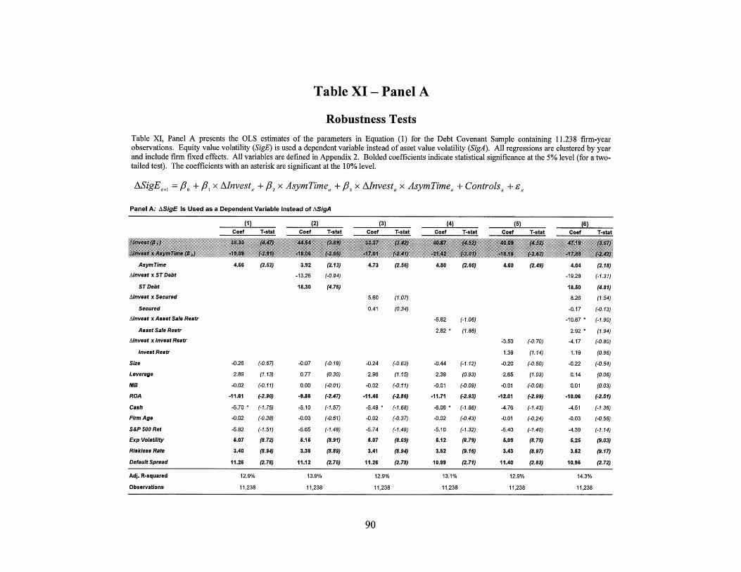
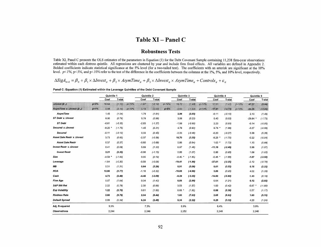
6. Robustness tests6.1. Using ASigA instead of ASigE6.2. Using an alternative measure of investment6.3. Using leverage instead of distress risk6.4. Partitioning by lease intensity6.5. Other robustness checks

7. ConclusionReferencesAppendices

Appendix 1: Examples of risk shiftingAppendix 2: Variable definitionsAppendix 3: Estimating SigA and DistressAppendix 4: Derivation of the optimal hedge equation

Figures 1 and 2Tables I - XI

1. Introduction

Risk shifting, also referred to as asset substitution in the finance literature, is an

investment distortion that benefits shareholders to the detriment of creditors. This study provides

empirical support for the hypothesis that high quality financial accounting information reduces

risk shifting by limiting the ability of managers to engage in suboptimally risky behavior.

Assuming that debtholders can foresee the management's actions, they will price protect

themselves by incorporating the expected losses from risk shifting (including the monitoring and

disciplining costs) into the price of debt ex ante. Since shareholders will ultimately bear the

costs of risk shifting, they will benefit from using a mechanism that can lower these costs

(Myers, 1977). I argue that pre-commitment to high accounting quality serves as a bonding

mechanism that allows shareholders to lower the agency cost of debt and to decrease the

deadweight loss.

Risk shifting was first introduced to the finance literature by Jensen and Meckling (1976)

and Galai and Masulis (1976) as a conflict of interests between shareholders and debtholders. It

involves managers, assumed to be acting in the interests of shareholders, switching to riskier

projects even though these projects may have a negative NPV for the firm. Such a shift in the

investment policy increases the value of the firm's equity, but decreases the value of debt. In

effect, risk shifting leads to a wealth transfer from debtholders to equityholders, which is

possible because the risk of investments is not shared equally between the two parties.

Shareholders capture most of the upside, while debtholders bear most of the downside due to the

asymmetric nature of their claims.1

1 Jensen and Meckling (1976) provide an analogy to risk shifting by comparing it to "the way one would play pokeron money borrowed at a fixed interest rate, with one's own liability limited to some very small stake."

Debtholders have an asymmetric payoff function that is capped at face value of debt, but

can go down to zero. Shareholders, on the other hand, have an unlimited upside potential but

cannot lose more than they have invested in the company due to the limited liability doctrine.

This asymmetry makes lenders more sensitive to increases than to decreases in default risk. This

idea can be best understood by treating shareholders' equity as a call option on the firm's assets

(Merton, 1974). The effect of a change in volatility of the underlying asset (i.e., firm's assets) on

the option value (i.e., the value of equity) increases as the value of the underlying asset decreases

relative to the strike price of the option (the firm's debt). That is, as the price of equity falls

lower and lower relative to the value of debt (i.e., as the firm becomes more and more

distressed), the potential gain to shareholders from shifting to higher-variance projects increases.

Consistent with this idea, a number of papers argue that the severity of risk shifting is

expected to be higher in firms with either high leverage (e.g., Jensen and Meckling, 1976; Smith

and Warner, 1979; Green and Talmor, 1986) or distress risk (e.g., Brealey, Myers, and Allen,

2006; Eisdorfer, 2008; Easton et al., 2009). However, there is also evidence that when a firm

becomes distressed, risk shifting may be offset by other incentives, such as risk management

(e.g., Guay, 1999; Purnanandam, 2008; Rauh, 2009), corporate tax minimization (Green and

Talmor, 1985), or by higher benefits from under-investment (Mao, 2003). In the end, it is an

empirical question whether the net benefit of risk shifting is higher in distressed firms.

I argue that high accounting quality as proxied for by asymmetric timeliness can help

mitigate risk shifting by improving debtholders' ability to effectively monitor the management's

actions and to discipline the managers when needed. Asymmetric timeliness is "the accountant's

tendency to require a higher degree of verification to recognize good news as gains than to

recognize bad news as losses" (Basu, 1997, p. 7). First, firms with high asymmetric timeliness

recognize bad news faster in financial reports, which gives debtholders more time to address te

issue. Second, asymmetric timeliness is expected to enhance the effectiveness of accounting-

based contractual restrictions on the managers' decision rights.

Asymmetric timeliness brings bad news forward and exerts a downward pressure on both

earnings and net assets thus making covenant violations more likely (Zhang, 2008). Early

recognition of bad news relative to good news sends a timely signal of distress to debtholders

and allows them more time for remedial actions. Besides, the incidence of a covenant breach

gives debtholders control rights necessary to take remedial actions, such are recalling the debt,

raising interest rates, or adding more covenants to existing contracts. In other words, violation of

a debt covenant provides creditors with a legally enforceable option to review and renegotiate the

debt contract, which improves debtholders' ability to monitor managers' actions efficiently and

to intervene quickly whenever warranted. An increase in accounting quality along this

dimension thus decreases the managers' ability to engage in risky investment behavior.

If accounting quality indeed plays a role in mitigating risk shifting, I expect it to dampen

the increase in business risk following new investments made by distressed firms. I proxy for

the change in the firm's level of risk using one-period-ahead changes in volatility of the firm's

asset values. I predict that investment corresponds to a lower increase in asset value volatility

when accounting quality is higher. I measure the degree of asymmetric timeliness in financial

reports (AsymTime) using a firm-specific measure of conditional conservatism (C Score)

developed by Khan and Watts (2009).

Several contractual mechanisms have been argued to reduce risk shifting. Convertible

debt allows debtholders to share in the upside potential, thus limiting shareholders' gains from

risk shifting (e.g., Jensen and Meckling, 1976; Green, 1984). Secured debt can limit risk shifting

since secured debtholders hold title to the collateral, making it impossible to sell the assets

without debtholders' approval (e.g., Smith and Warner, 1979). Issuing short-term debt can be

another solution, since having the debt mature before an investment is undertaken eliminates the

incentives for shareholders to engage in risk shifting (Myers, 1977; Barclay and Smith, 1995).

Eisdorfer (2008) provides empirical evidence that risk shifting still exists in distressed firms

despite the presence of these three contractual mechanisms.

Including restrictive covenants in debt contracts is another important commitment device

that can be used to reduce risk shifting (Smith and Warner, 1979). While shareholders prefer not

to have covenants restricting firm's investment choices ex post, they accept these covenants ex

ante to rule out future actions that may increase shareholders' value in the short run (e.g., risk

shifting) but that will eventually lead to a deadweight loss to the firm (Myers, 1977). I control

for the presence of the mechanisms described above using the data on public and syndicated debt

issues available from the Fixed Investment Securities Database (FISD) and the Securities Data

Corporation (SDC).

I also test a number of cross-sectional and time-series predictions. I expect the usefulness

of accounting information for lenders to vary cross-sectionally with the richness of the firm's

information environment, the level of distress risk, the availability of cash, and the source of debt

(public versus syndicated). I also expect time-series variation based on whether observations

belong to the time periods before or after the adoption of the Sarbanes-Oxley Act of 2002

(SOX). I proxy for the richness of information environment using the average daily bid-ask

spread, the number of analysts following the firm, and the adjusted PIN score (from Duarte and

Young, 2009). I use changes in implied asset volatility from the Merton (1974) model as a proxy

for changes in business risk. I use cash flow from operations to proxy for the strength of risk

shifting incentives due to the ease with which cash can be converted into riskier assets.

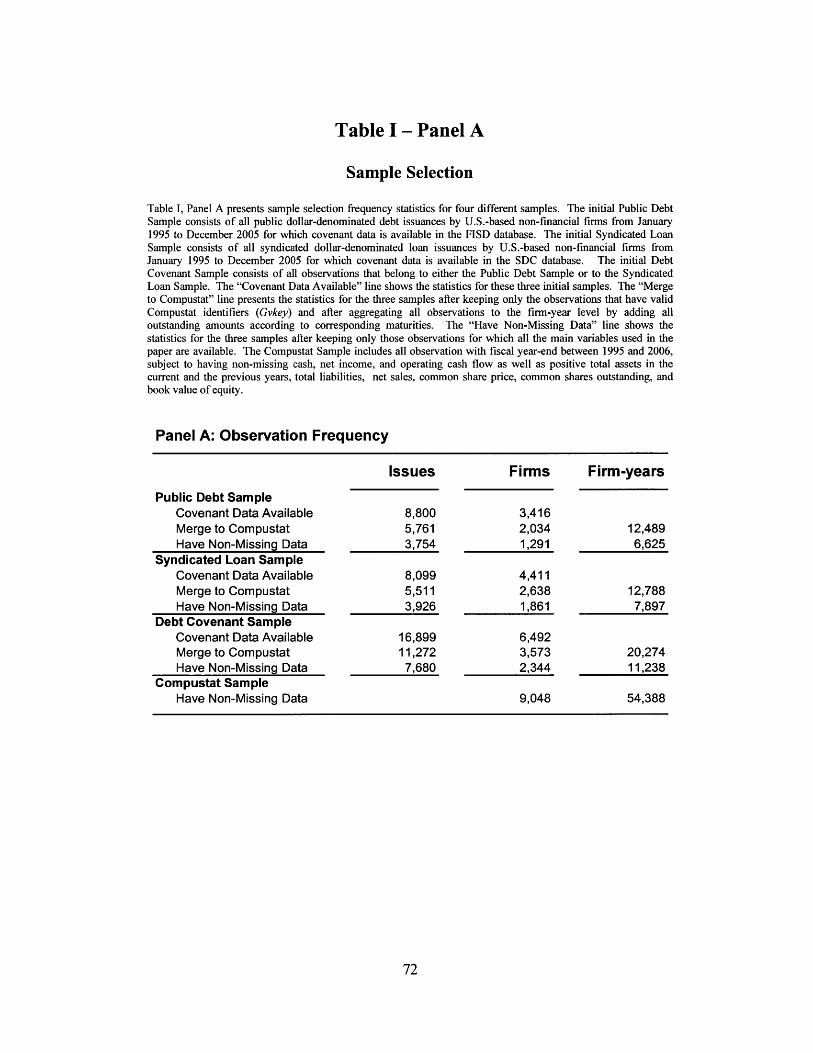
I combine several databases to obtain a sample containing contract-specific information

on outstanding public and private debt with financial and accounting data (the Debt Covenant

Sample). The final sample includes 11,238 firm-year observations and 2,344 individual firms

between 1995 and 2006 and is collected by intersecting publicly available financial information

from Compustat and CRSP with data on public debt issues and syndicated loans. I gather data

on public debt issues from the Mergent Fixed Investment Securities Database (FISD) and data on

syndicated loan deals from the Securities Data Corporation (SDC) database.

The results support the hypothesis that accounting quality reduces risk shifting. The

sensitivity of volatility changes to new investments decreases by a half when a firm moves from

the lowest accounting quality decile to the highest accounting quality decile. I control for the

presence of the contractual mechanisms that have been argued to reduce risk shifting (i.e., short-

term debt, convertibility, secured debt, and restrictions on asset sales and capital expenditures).

The effect of accounting quality on risk shifting also appears to be stronger in firms with poor

information environment and in firms with public debt. I also find that the effect of accounting

quality on risk shifting (as well as the risk shifting behavior itself) is present only in the two top

distress quintiles.

The results are robust to alternative proxies for firm riskiness, investment intensity, the

level of distress risk, and alternative financing arrangements (leases). I also control for firm- and

market-specific characteristics that have been shown to affect future volatility, investment, and

accounting quality. The results are consistent with the prediction that firms with high accounting

quality exhibits fewer signs of risk shifting.

This study contributes to the understanding of the effects of accounting information on

business decisions. I explore a specific debt-equity agency conflict, risk shifting, and show that

accounting quality can improve investment efficiency by preventing firms from engaging in

suboptimally risky activities and thus can reduce deadweight losses. A number of recent papers

examine whether various accounting quality dimensions can mitigate agency conflicts (e.g.,

LaFond and Watts, 2008; Zhang, 2008, Louis et al., 2009) and improve investment efficiency

(e.g., Biddle and Hilary, 2006; Biddle et al., 2008; Francis and Martin, 2008). The results in this

study are consistent with and complement this line of research.

While many papers concentrate on the effects of accounting quality on the profitability of

investments (the first moment of the return distribution), I focus on the effect of accounting

quality on the riskiness of investments (the second moment of the return distribution). Most of

modern finance theory depends on the assumption that the mean and the variance are the only

two properties of the return distribution that investors use to solve their portfolio optimization

problem. Thus, changes in the level of risk have value implications for investors. This study

shows that accounting quality can prevent firms from making suboptimally risky investments

and incurring deadweight losses by enhancing the monitoring and disciplining mechanisms

available to debtholders.

The rest of the study is organized as follows. Section 2 provides some background on

risk shifting and motivates the role accounting quality plays in mitigating this investment

distortion. Section 3 explains model specifications, and the measures of accounting quality and

distress risk. Section 4 presents the sample selection procedure and descriptive statistics.

Section 5 discusses the empirical results while Section 6 describes the robustness tests. Section 7

offers potential extensions and concludes.

2. Hypothesis Development

2.1. Incentives and consequences of risk shifting

Risk shifting occurs when managers substitute away from lower risk assets or strategies

toward riskier ones. In effect, risk shifting involves a wealth transfer from debtholders to

shareholders as a result of risky investment decisions.2 This transfer is possible because the

upside and the downside potentials of risky investment are not shared equally among

shareholders and debtholders. Shareholders capture most of the upside of high-risk activities

while debtholders absorb most of the downside.3 At maturity, lenders receive at most the face

value of debt.4 The payoff, however, may be less than the face value if the value of the firm's

assets is insufficient to cover the principal. Due to limited liability, debtholders cannot recover

anything from shareholders beyond the value of the assets. In contrast, shareholders may also

lose up to one hundred percent of their investment, but their payoff is not bounded from above.

Debt-equity agency conflicts arise only when a firm has risky debt. When the possibility

of default is virtually zero, "debtholders have no interest in income, value or risk of the firm"

(Myers, 2001, p. 96). Debt payoff function is flat in this region and small changes in the firm's

economic outlook do not affect the value of debt. However, when there is a possibility that the

2 Risk shifting is usually caused by managers over-investing in risky projects. On certain occasions, however, riskshifting can result from under-investing. In case of an airline, for instance, under-investing in such projects asrequired repairs and maintenance can make airplanes less reliable and cause the operations to become more riskythus subjecting the company to a higher probability of accidents and lawsuits. Not purchasing enough insurancemay have a similar risk-increasing effect.3 This may not always be the case, even for investors holding plain vanilla bonds. The fast growth of creditderivatives has created the so-called "empty creditor" problem (Hu, 2009). Credit default swaps allow lenders todecrease or even eliminate the default risk associated with their debt investment. In fact, a lender may have a shortexposure to the borrower's credit quality if the former holds more credit default swaps than debt claims on theborrower's assets. Since the lender will benefit if the borrower defaults on its obligations, the former may beincentivized to push the latter toward default even though such an outcome would be undesirable for both parties inthe absence of credit default swaps.4 Whereas the payoff at maturity is typically fixed at face value, the value of debt may be higher than the face valueat some point prior to maturity. For instance, a steep decrease in interest rates may cause certain coupon bonds tosell above par. In addition, interest-decreasing performance pricing provisions commonly used in bank debt asdocumented by Asquith et al. (2005) often allow for the reduction of the rate of interest of debt if the borrower'scredit quality has improved. This may also make the value of bank debt higher than the final maturity payoff.

debt will not be repaid in full at maturity, shareholders can gain at the expense of debtholders.

Being rational, debtholders take into account the shareholders' incentives to engage in risk

shifting after entering into the debt contract and price protect themselves. Since they are the

residual claimants, shareholders bear the cost of risk shifting by paying a higher interest rate on

debt to compensate debtholders for the expected losses due to suboptimal investment behavior as

well as for the costs debtholders expect to incur for additional monitoring and disciplining.

Black and Scholes (1973) and Merton (1974) pioneered the view of the firm's capital

structure using an option-pricing framework. The payoff structure of debt, for example, can be

replicated by taking a long position in the firm's assets and a short position in a call option on

these assets with the strike price that equals the face value of debt and the maturity that equals

the maturity of debt (assuming, for simplicity, that it is a zero-coupon debt). Under the law of

one price, debt value should equal the value of assets less the value of the call. Viewing capital

structure within the option-like framework makes it clear that increasing the volatility of assets,

ceteris paribus, will cause the value of equity to increase and the value of debt to decrease.5

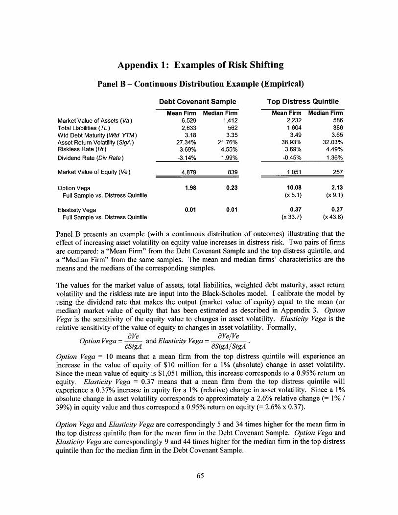
Appendix 1, Panel A presents a hypothetical example of how increasing asset volatility

benefits equityholders to the detriment of debtholders. The example also demonstrates that the

same (or proportional) increase in asset volatility produces more benefits for shareholders of a

more risky firm. Appendix 1, Panel B illustrates a similar idea in a continuous-time setting using

the empirical data from the sample used in this study. Two pairs of firms are compared: the two

"mean firms" possess the mean characteristics of the main sample used in this study (the Debt

5 A caveat regarding the use of option-pricing models to examine the firm behavior is warranted. Jensen andMeckling (1976) and Smith and Warner (1979) note that the option pricing analysis assumes that the value of thefirm (debt and equity) is independent of its capital structure, which may not be the case if debt covenants arepresent. The option pricing analysis also ignores endogeneity in stockholders behavior by treating the incidence ofdefault, as well as the value and the volatility of the firm's assets as exogenous rather than as decision variables.

Covenant Sample) and of the top distress quintile of this sample while the two "median firms"

have the median characteristics of the two above-mentioned samples.

As stated in Appendix 1, the total change in the value of the call option (i.e., the market

value of equity) for a small change in volatility (of assets) is maximized at a point where the

value of the call option equals the strike price (i.e., the face value of debt). Similarly, the

percentage change in the value of the call for a small percentage change in volatility is

maximized when the value of the call is small relative to the value of the strike price. Thus, the

value transfer from debtholders to equityholders resulting from risk shifting is highest when the

value of assets is close to the face value of debt or is far below it, depending on which option

sensitivity measure is used. Regardless of the measure used, both maxima lie in the region when

the probability of the firm defaulting on its obligations is relatively high.

Consistent with this idea, a large stream of literature in finance examines risk shifting as

an important cost of financial distress that is relevant to firms with risky debt. All else equal, the

severity of risk shifting is expected to be higher in firms with more risky debt. Two proxies for

the strength of risk shifting incentives are typically used: a) high leverage (e.g., Jensen and

Meckling, 1976; Smith and Warner, 1979; Green and Talmor, 1986); and b) high default risk

(e.g., Brealey, Myers, and Allen, 2006; Eisdorfer, 2008; Easton et al., 2009).

At the same time, a number of papers argue that risk shifting does not monotonically

increase in leverage (e.g., Gavish and Kalay, 1983; Bhanot and Mello, 2006) or that it is offset

by other incentives prevalent in distressed firms such as risk management (e.g., Guay, 1999;

Purnanandam, 2008; Rauh, 2009) and corporate tax minimization (Green and Talmor, 1985), or

by higher benefits from under-investment (Mao, 2003). In fact, some researchers argue that risk

shifting effects may be small or insignificant (e.g., Andrade and Kaplan, 1998; Parino and

Weisbach, 1999). Besides, debtholders in distressed firms are more likely to have stronger

control rights than their counterparts in financially healthy firms (e.g., Nini et al., 2009-b) and

thus can exert more pressure on the firm to abstain from suboptimal investment decisions. Thus,

it is an empirical question whether the net benefit of risk shifting is higher in distressed firms.

Empirical evidence is consistent with the presence of risk shifting in financial firms.

Brown et al. (1996) and Brown et al. (2001) find that mutual and hedge fund managers,

respectively, take more risk in the second half of the year if their portfolio experienced sub-

standard performance in the first half of the year. Evidence on risk shifting in non-financial

firms is sparse, possibly due to the fact that the market value of assets is not directly observable,

which makes estimating asset volatility difficult. Recent research shows that the effect of risk

shifting on the value of debt is non-trivial. Eisdorfer (2008) examines the relation between

volatility and investment in distressed firms and finds that the value of debt may be reduced by

as much as 6 percent as a result of risk-shifting behavior in high-volatility periods. He measures

asset volatility of non-financial firms by using the Merton (1974)-inspired option-based

framework (described in Appendix 3) and infers asset value and volatility from the value and

volatility of equity.

2.2. Mechanisms that reduce risk shifting

Rational debtholders recognize managers' incentives and incorporate value implications

of managers' future actions into the price of debt. On average, debtholders will not suffer losses

from suboptimal corporate decisions unless they consistently underestimate the effects of such

decisions (Jensen and Smith, 1985). In the end, it is shareholders who bear the agency costs of

debt by paying higher interest rates than they would if they could credibly commit to abstaining

from risk shifting activities. Therefore, it is beneficial for shareholders to pre-commit to

constraints ex ante that will rule out certain behavior even though such actions may be rational ex

post (Myers, 1977). Prior research has identified several contractual mechanisms that may limit

risk shifting6 .

Convertible debt is a hybrid security that allows debtholders to share in the upside

potential, thus limiting shareholders' gains from risk shifting (e.g., Jensen and Meckling, 1976;

Smith and Warner, 1979; Green 1984; Jensen and Smith, 1985; Eisdorfer, 2008). The

conversion option is like a call option written by equityholders to debtholders, whose value

increases in the volatility of assets. A decrease in the value of straight debt will be (at least

partially) offset by an increase in the value of the option component. Since shareholders are

short this call option, their incentives to increase asset volatility are lower. Convertible debt,

however, has a cost. Its presence may exacerbate the under-investment problem (Smith and

Warner, 1979) as well as have adverse tax consequences due to the closeness of convertible debt

to equity from the tax authorities' point of view.

Secured debt can also limit risk shifting since secured debtholders hold title to the

collateral, making it impossible to sell these assets without debtholders' approval (e.g., Smith

and Warner, 1979; Eisdorfer, 2008). Collateralizing an asset, i.e., issuing debt secured by an

asset, also reduces expenses in case of foreclosure (Smith and Warner, 1979). The costs

associated with secured debt include additional out-of-pocket costs such as administrative

expenses and opportunity costs arising from restricting the firm from taking advantage of an

opportunity to dispose of collateral at a gain.

6 As discussed in Smith and Warner (1979) and Jensen and Smith (1985), debt-equity conflict cannot be solved bysimply passing control of the firm to debtholders. First, bondholders would then have incentives to engage in"reverse risk shifting" by choosing suboptimally safe projects. Second, the degree of control debtholders can havein a firm is limited by common or statutory laws such as the Securities Act of 1934 and by the Trust Indenture Actof 1939.

Issuing short-term debt can be another solution if the debt matures before an investment

is undertaken, eliminating the incentive for shareholders to engage in risk shifting (Myers, 1977;

Barclay and Smith, 1995; Parrino and Weisbach, 1999; Eisdorfer, 2008). Using short-term debt

instead of borrowing long-term provides debtholders with opportunities to adjust the terms of the

contract based on the borrower's performance.' Suppose a firm borrows money to design a new

production process that can be made more or less risky. If the debt is renegotiated before the

completion of the project, creditors will be able to price the new debt according to the level of

the riskiness of the process chosen by the firm. This setup effectively eliminates the

shareholders' ability to extract value from the debtholders. Such a strategy, however, may be

costly due to high renegotiation and administrative costs.

Including restrictive covenants in debt contracts is yet another contractual device that can

be used to reduce risk shifting. Smith and Warner (1979) argue that restrictions on investment,

disposition of assets, and M&A activity can mitigate risk-shifting. The contracting parties can

also incorporate affirmative covenants 8 into debt contracts to decrease the potential for risk

shifting. Smith and Warner (1979) note that a violation of an affirmative covenant provides a

signal to the lender that can result in renegotiation of a debt contract. Current evidence confirms

the frequent use of debt covenants to protect debtholders' investment (e.g., Dichev and Skinner,

2002; Billett et al., 2007; Chava and Roberts, 2008; Nini et al., 2009-a; Roberts and Sufi, 2009).

Verde (1999) provides evidence that the two major functions of debt covenants are a)

preserving seniority and collateral; and b) ensuring that borrowers' actions are aligned with

lenders' interests as long as the debt is outstanding. For example, many bank loan agreements

7 Put differently, issuing debt with shorter maturity reduces managers' incentives to engage in risk shifting becausethe value of a shorter call option is not as sensitive to changes in the volatility of asset returns.8 An affirmative covenant is a clause in a debt contract that requires that firms take certain actions such as holding acertain amount of particular assets (e.g., cash), maintaining the firm's properties in good condition, or keepingcertain metrics (mainly accounting-based) above pre-specified thresholds.

restrict asset sales outsides of the firm's regular course of business as well as contain cash flow

sweeps requiring the borrower to apply the proceeds from asset sales toward the reduction of

senior debt.

The mechanisms discussed above, however, cannot fully eliminate shareholders'

incentives and ability to engage in risk shifting. First, since the investment set is not directly

observable and cannot be directly contracted upon, it is nearly impossible, as well as inefficient,

to control all of the firm's investment and production decisions. 9 Second, an innovation in the

production technology that may not have existed when the debt was issued, can lead to

significant changes in the firm's risk profile. As a result, restrictive covenants are not perfectly

efficient in constraining risk shifting. Third, all of these mechanisms have attendant costs. In

addition to renegotiation and administrative costs, firm value may also be affected by lost

opportunities due to covenant tightness and debt security provisions over-restricting managers'

choices. Therefore, a mechanism that enhances the degree of "contract completeness" or reduces

these costs would benefit both the borrower and the lender.

2.3. Role offinancial reporting

I argue that accounting quality complements other mechanisms that debtholders use to

control agency conflicts. Several papers (e.g., Bushman and Smith, 2001; Lambert et al., 2008)

suggest that high accounting quality can increase investment efficiency by improving the

coordination between firms and investors. 10 Bushman and Smith (2001, p. 295), for example,

argue that "financial accounting information is a direct input to corporate control mechanisms

9 The absence of complete markets is necessary in order for agency conflicts to have any effect on the behavior ofthe parties involved. If market were complete, the agency problem could be solved through state-contingentcontracts.10 Improving investment efficiency also includes increasing the productivity of assets in place or human capital.

designed to discipline managers" to direct resources toward their most productive use and to stop

managers from expropriating wealth from investors.

Empirical evidence indicates that high accounting quality does indeed mitigate

information asymmetry between managers and outside investors, thus improving project

selection and lowering the cost of raising funds. Biddle, Hilary, and Verdi (2008) show that high

accounting quality mitigates both under- and over-investment and increases firm profitability by

aiding firms in the selection of more profitable projects. Bushman et al. (2006) provide cross-

country evidence by showing that countries with a higher degree of a timely accounting

recognition of economic losses (a measure of accounting quality) respond faster to declining

investment opportunities by reducing the flow of capital to new investments.

Ball et al. (2008) argue that the recognition of financial information is more important to

debtholders than to shareholders. They argue that such an asymmetry in demand exists due to

differences in the way information affects the claimants' control rights. Upon receiving new

information, shareholders can exercise their control rights via the board of directors.

Debtholders, on the other hand, do not have direct means of influencing the firm's actions unless

the firm violates a debt covenant, which provides debtholders with an option to assume control

rights. Since most debt covenant thresholds are based on pre-specified accounting numbers,

publicly available information that is not in the financial statements and has not otherwise been

contracted upon does not provide debtholders with the controls rights necessary to influence the

firm's actions.

Accounting quality is an inherently subjective concept and many attempts have been

made to define and quantify it (e.g., Francis et al., 2004, Barth et al., 2008). SFAS No. 2, for

example, considers timeliness, relevance, verifiability, reliability, unbiasness, comparability, and

consistency to be desirable properties of financial reporting and disclosure information. Various

parties, however, are likely to be interested in different dimensions of accounting quality based

on the nature of their claims and contractual arrangement with the firm.

2.4. Dimension of accounting quality important to debtholders

Debtholders are interested in the dimensions of accounting quality that provide them

with a credible signal of impending distress and help them take remedial actions. Due to the

asymmetric nature of their claim's payoff, debtholders are more sensitive to increases than to

decreases in default risk and tend to focus on the left tail of the earnings and net assets

distributions. As a result, debtholders are typically more interested in receiving bad news than

good news about the firm. However, if the value of the firm's assets falls far below the value of

its debt, the importance of good news to debtholders also increases.

This idea is illustrated in Figure 1, which depicts a payoff diagram of a zero-coupon

debt as a function the market value of assets (Va) at debt maturity. The value of assets can fall

into two regions. The high-risk region captures the states of nature where the expected value of

assets at debt maturity is closer to (or less than) the face value of debt (F) and thus the

probability that the market value of assets will be below the face value of debt at debt maturity is

non-trivial.1" Debtholders in this region pay significant attention to the news about the firm since

the value of their debt investment is sensitive to changes in the firm's economic outlook.

In the low-risk region, the value of assets is significantly higher than the face value of

debt and the probability that Va will be less than F at debt maturity is small. Debtholders in this

1 It is important to remember that according to the option-pricing framework for valuing equity, the probability ofdefault is a function not only of asset value, but also of other standard parameters in the Black-Scholes-Mertonequation. As a result, two firms having the same value of assets and face value of debt may have different defaultprobabilities due to differences in other determinants of default risk (e.g., asset volatility and debt maturity).

region are not concerned about the value of their claims as much and, consequently, the value of

debt will vary less in response to news about the firm. Their payoff function is almost flat in this

region, i.e., debtholders are very likely to receive the face value of their debt investment back at

maturity regardless of the value of assets. As a result, debtholders in this region are not as

sensitive to either good or bad news since small changes in profitability, value, or risk profile of

the firm do not affect their expected payoff at debt maturity.

The relative importance of good and bad news for debtholders varies at different points

along the default spectrum. When the market value of assets is significantly below the face

value of debt, the market value of debt becomes almost symmetrically sensitive to increases and

decreases in the market value of assets and debtholders are concerned about the timeliness of

both good and bad news. As the market value of assets increases, so does the importance of bad

news relative to good news. Since debt payoff at maturity cannot exceed its face value, the

market value of debt asymptotes to the face value but never crosses it, no matter how high the

market value of assets is. On the other hand, if the company is performing poorly, the expected

payoff to debtholders and the market value of debt fall as the market value of assets decreases

(all the way down to zero, in extreme cases). Thus, if the asset value is high enough, a positive

economic shock does not increase the value of debtholders' claims by much, while a negative

economic shock can erode this value considerably.

I operationalize the idea of a differential demand from debtholders for good and bad news

by using the asymmetric timeliness in the recognition of good versus bad news. 12 Asymmetric

timeliness puts downward pressure on earnings and net assets, which brings bad news forward

relative to good news and assures investors that gains are not overstated and losses are not

12 Asymmetric timeliness is "the accountant's tendency to require a higher degree of verification to recognize goodnews as gains than to recognize bad news as losses" (Basu, 1997, p. 7).

understated (LaFond and Watts, 2008). Managers may withhold bad news to conceal problems

and prevent creditors from forcing the firm into reorganization or bankruptcy. These incentives

are especially strong for distressed firms. Graham et al. (2005) find that poorly performing firms

delay the recognition of bad news hoping that the firm's health will improve in the future. 13

Healthy firms can also delay recognizing bad news to give themselves time for in-depth analysis,

interpretation, and consolidation of bad news into larger news releases (Kothari et al., 2009).14

Asymmetric timeliness can reveal a shift in investment policy from safe, positive-NPV

projects towards risky, negative-NPV ones by committing the management to recognizing the

losses on new risky projects early (Ball and Shivakumar, 2005). Asymmetric timeliness can also

help debtholders in detecting risk shifting even if new risky projects have a positive NPV.

Arguably, this happens because as the volatility of an average project increases, so does the

probability of a loss on this project (assuming the expected payoff increases less than volatility).

Asymmetric timeliness increases the effectiveness of debt contracts by enhancing the

positive effects of creditor intervention following an incidence of covenant violation. 15 Zhang

(2008) finds that firms with a high degree of asymmetric timeliness are more likely to violate

debt covenants due to the downward effect of asymmetric loss recognition on earnings and net

assets, the metrics that are commonly used in covenants (e.g., current ratio, net worth, debt to

equity, etc). A timely covenant violation sends an early signal of potential distress to

debtholders and gives them an option to review and renegotiate the debt agreement if necessary.

13 In their survey answers, most CFOs state that the management of a growing firm hopes that future earningsgrowth will offset reversals from past earnings management decisions (Graham et al., 2005).14 Some researchers have argued that managers may release bad news faster than good news to promote reputationfor transparent reporting or to avoid potential lawsuits (e.g., Skinner, 1994 and 1997).15 Not all researchers agree with this point of view. Gigler et al. (2009, p. 768), for instance, provide theoreticalevidence that "under very plausible conditions, we find that accounting conservatism, which affects the informationcontent of accounting reports, actually decreases the efficiency of debt contracts."

By enhancing the timeliness of covenant violations, asymmetric timeliness speeds up the transfer

of control rights from shareholders to debtholders. 16

A typical debt covenant gives debtholders a legally enforceable right to demand an

immediate debt repayment or an option to renegotiate the debt contract in case of a technical

default. 17 Several papers show that such a transfer is an important contracting mechanism that

can be used to reduce risk shifting and to improve operating performance. Chava and Roberts

(2008) provide evidence that violations of the net worth and current ratio covenants lead to

debtholders limiting the firm's future capital expenditures. Nini et al. (2009-b) corroborate these

findings by showing that capital expenditure restrictions cause companies to lower actual

expenditures following a technical default, which leads to lower value-dissipating investments

and, as a result, to better performance and higher market values.

Cross-default provisions, that are common in public debt agreements, enhance the effect

of asymmetric timeliness on the risk-shifting behavior. A typical cross-default provision clause

in a debt covenant stipulates that a default on any of the company's outstanding loans will trigger

a default on all of the company's loans. This feature provides an extra benefit to the lender by

giving it more opportunities for contractual intervention and loan renegotiation if the company

breaches a covenant in any of its debt agreements. For example, if the borrower breaches a net

worth or a current ratio covenant on a loan from one lender, other lenders also receive the option

to review and renegotiate their debt agreements. Cross-default provisions are especially

important for public debtholders since public debt agreements contain fewer covenants that are

more loosely set then do private debt agreements (e.g., Bradley and Roberts, 2004).

16 It is important to notice that it is asymmetric timeliness and not just bad news timeliness that is important todebtholders. First, affirmative covenants are violated by losses and not by gains. Second, asymmetric timelinessprevents managers from recognizing gains early in order to cover up some of the losses.17 While empirical evidence shows that debtholders waive technical defaults in the majority of cases (e.g., Dichevand Skinner, 2002), they have a valuable option to influence management's decisions.

For accounting quality to affect risk shifting, there should be an equilibrium mechanism

that ensures that firms that commit to a certain level of accounting quality ex ante do not renege

on their promises ex post.1 8 Prior literature has identified several such mechanisms that can

arguably prevent firms from changing the level of asymmetric timeliness in their financial

reports. First, contracting mechanisms, such as the use of"fixed GAAP" in covenants (Beatty et

al., 2002) help borrowers commit to a pre-debt level of asymmetric timeliness. Many debt

covenants also contain provisions expressly prohibiting firms from changing accounting methods

or requiring detailed explanations of such changes. For example, the borrower may not be

allowed to change from the double-declining to the straight-line depreciation method or will

have to disclose the reasons for such a change in detail.

Second, reputation is another mechanism that helps keep borrowers from deviating from

their ex ante accounting choices. Since accessing capital markets is a multi-period game, the

ability of a company to obtain financing on favorable terms depends on its relationship with the

lenders. Borrowers who choose to benefit short-term from changing their accounting quality

may face negative reputational consequences in the future. They can find it more difficult and

expensive to obtain future financing from the lenders if the latter cannot trust that the borrowers

will keep the choices to which they have pre-committed before entering into the debt contract.

A third factor that can help keep borrower at the ex ante level of asymmetric timeliness is

the threat of auditor litigation that is fairly common in practice. As the probability of default and

potential bankruptcy rises, so does the auditor's exposure to litigation (Kothari et al., 1988; Lys

and Watts, 1994; Watts, 2006). The auditor liability further increases when it becomes apparent

18 Debtholders are not really concerned if managers of distressed firms become more conservative in their financialreporting choices. Lenders can always choose to ignore the distress signal or a covenant violation if they believe thefirm's operations are fundamentally sound. Dichev and Skinner (2002) and Nini et al., (2009-b), among others,provide evidence that covenant violations are quite common and argue that the vast majority of them are waived.

that the firm has failed to disclosed all relevant bad news in a timely fashion (Skinner, 1997).

Prior research has documented that auditors adjust their audit plan and increase the issuance of

modified opinions as the probability of client default and litigation risk increase (Pratt and Stice,

1994). These findings suggest that auditors are likely to oppose any attempts by their clients to

lower the level of asymmetric timeliness in their financial statements as default risk increases.

2.5. Predictions

Risk shifting involves managers taking high-risk (possibly negative-NPV) projects that

increase the value of equity but decrease the value of debt. Eisdorfer (2008) finds that the

relation between expected volatility and investment intensity is positive for distressed firms and

interprets this as evidence of risk shifting behavior. I hypothesize that asymmetric timeliness can

mitigate this relationship and predict that this effect is reflected in the one-period-ahead changes

in asset value volatility in response to new corporate investments. New investments should then

correspond to a decrease in asset volatility for firms with higher levels of asymmetric timeliness

relative to those with lower levels of asymmetric timeliness.

I expect asymmetric timeliness to decrease risk shifting by making covenant violations

more timely, thus providing debtholders with an earlier signal of poor performance and allowing

them more time for remedial actions. A covenant violation gives creditors a contractual right to

intervene if necessary and stop the management from engaging in wealth-dissipating activities.

Thus, higher asymmetric timeliness will benefit debtholders by decreasing the firm's ability to

engage in risk shifting and, in the long-run, will also benefit shareholders by reducing the

deadweight loss they incur as a result of their risk shifting incentives.

HI: Risk-shifting behavior decreases in accounting quality.

Financial reporting is just one of the sources of information about the firm. Stock market

and information intermediaries such as analysts are other important sources that can also provide

valuable information to investors and decrease the importance of financial reporting as a

mechanism for mitigating debt-equity agency conflicts. If alternative sources of information are

unavailable or if the information they provide is very noisy, accounting quality becomes an

important communication channel between the company and investors. As a result, I expect that

accounting information will be important for firms with poor information environments.

I proxy for the richness of information environment by partitioning the sample using four

proxies: a) the cross-sectional median of the average daily closing bid-ask spread (scaled by the

closing price) over the past year; b) the cross-sectional median of the average number of analysts

that followed the firm over the past year; c) the cross-sectional median of the adjusted

probability of informed trading (AdjPIN) score from Duarte and Young (2009).

H2: Accounting quality has a stronger effect on risk shifting when the firm's

information environment is poor.

Risk shifting is not costless. First, substituting one asset for another inevitably involves

transaction costs. Second, increasing the business risk may increase the probability of future

lawsuits against the firm. Third, risk shifting has opportunity costs. There are other ways

equityholders can extract value from debtholders, such as excessive dividends payouts. The

funds that are spent on risk shifting projects become unavailable to shareholders until the payoffs

from the project are realized. Firms will engage in risk shifting only when the value transferred

to equityholders exceeds the costs of risk shifting. Since the increase in the value of equity in

response to increases in risk rises with the level of distress, I expect that risk shifting behavior

will be stronger among firms in top distress quintiles. While this expectation is in line with an

established body of finance literature, some researchers make an argument that risk shifting may

be non-monotonic in distress risk or leverage (see Section 2.1. for more discussion on this issue).

To examine the effect of distress on the relation between accounting quality on risk shifting, I

estimate Equation (1) separately for the five quintiles partitioned on distress risk.

H3: The effect of accounting quality on risk shifting increases in distress risk.

Since cash is usually the safest and the most liquid asset, the easiest way for a firm to

engage in risk shifting is to use cash to buy a riskier asset. If the acquired asset is sufficiently

risky, this action will benefit shareholders but hurt debtholders. Therefore, all else equal, it is

easier for firms with more available cash to engage in risk shifting. This argument is the

extension of an idea from Jensen (1986) that excess cash can negatively affect investment

efficiency. Another way equityholders may want to use extra cash is to pay themselves a high

dividend. However, this option is often unavailable due to debt covenants restricting dividends

as well as due to the possibility of having such a payout deemed a fraudulent conveyance and

having it clawed back by the bankruptcy court.

Several studies use the presence of cash as a proxy for agency conflicts and information

asymmetry. Chava and Roberts (2008), for instance, find that the changes in investment are

larger for firms with more cash following a covenant violation. Since risk shifting is expected to

be less of a problem in firms with low cash, accounting quality may be less important for

debtholders in this setting. I hypothesize that risk shifting behavior and the demand for high

quality accounting information is higher for distressed firms with higher cash flows.

H4: Accounting quality has a larger effect on risk shifting among distressed firms

when CFO is high.

Diamond (1991) characterizes the U.S. debt markets as a continuum of access to

monitoring and private information with bondholders being at the low end of the spectrum and

banks being at the high end. Since public debt provides debtholders with limited ability to

monitor borrowers, accounting quality is an important information source for them. Banks, to

the contrary, have access to private information and can restrict suboptimal investment activities

via loan covenants. As a result, they may not be as dependent on accounting quality as a

monitoring and disciplining mechanism.

On the other hand, prior research has shown that private debt agreements contain more

covenants and these covenants are also tighter and more detailed than those in public debt

agreements (e.g., Verde, 1999; Bradley and Roberts, 2004). Roberts and Sufi (2008), for

instance, show that 96% of all private debt agreements have a financial covenant. Thus,

covenant violations, the primary mechanism through which accounting quality is expected to

affect risk shifting, are expected to be more common in private debt. Besides, creditor

intervention and renegotiation is likely to be more efficient for firms with private debt (Roberts

and Sufi, 2008).

At the same time, most public debt has a cross-default provision (80% of observations in

the Public Debt Sample described in Table I, Panel C have a cross-default provision), that allows

bondholders to piggyback on covenant violations in private debt contracts. Thus, the effect of

the source of debt on accounting quality seems to be ambiguous. I do not make a directional

prediction regarding the strength of the relationship between accounting quality and risk shifting

based on the source of debt.

Hs: The effect of accounting quality on risk shifting varies with the source of debt.

Several papers examined the effects of the Sarbanes-Oxley Act (SOX) adopted in late

July of 2002 on corporate risk taking (e.g., Bargeron et al., 2009; Cohen et al., 2009). SOX

introduced a number of corporate governance reforms, including certification requirements and

severe penalties for top managers in case of fraud, independent audit committees, more rigorous

internal controls, extensive disclosure regulation, etc. Bargeron et al. (2009) find that several

measures of risk-taking decline among U.S. firms relative to a control group of non-U.S firms

after the passage of SOX. Cohen et al. (2009) similarly find that the decline in risky investments

in the post-SOX period exceeds what would be expected from changes in managers'

compensation.

At the same time, one of the primary goals of SOX was to increase the provision of more

timely and reliable information to internal and external parties (Dey, 2009). This fact, together

with financial statements certification requirement and criminal penalties for C-level officers for

misrepresentation, arguably led to more dependable accounting numbers. Since risk shifting is a

subset of risk-taking activities, I hypothesize that the passage of SOX has decreased risk shifting

behavior in non-financial firms and increased the role of accounting quality as a mitigating

mechanism. Since SOX was adopted in late July of 2002, I divide the sample based on whether

the fiscal year-end falls before versus after July 31, 2002 and examine the difference between the

strength of evidence of risk shifting and accounting quality effects.

Any evidence of the effects of SOX has to be interpreted with caution since a number of

confounding events that could have affected both the firm's risk-taking and the information

environment took place in the U.S. close to the passage of SOX. The passage of Regulation Fair

Disclosure (Reg FD) in October 2000 and a series of high-profile corporate scandals starting

from the fall of Enron in December 2001 are two examples of such events (Dey, 2009). Reg FD

could have altered the firm's information environment by effectively preventing managers from

using analysts as a channel for incorporating news into stock prices. The fall of Enron (together

with other corporate scandals) caused the loss of confidence in accounting information and

encouraged market participants to exercise more effort in monitoring and disciplining managers.

H 6: Risk shifting decreases and the mitigating effect of accounting quality increases

after the passage of SOX.

An important working assumption made in this study is that managers interests are

aligned with the interests of shareholders and that the former will act in the benefit of the latter.

Prior research has shown that this may not always be the case and that to protect their human

capital and private benefits of control, managers may act more conservatively than shareholders

would desire. This has been shown both theoretically and empirically (e.g., Hirshleifer and

Thakor, 1992; Eckbo and Thorburn, 2003). The less diversified managers' human capital is and

the more important the private benefits of control are for managers, the more risk averse they are

likely to be in setting corporate investment policy (John et al., 2008).

Eisdorfer (2008) tests whether the extent to which managers' and shareholders' interests

are aligned affects the strength of the relationship between financial distress and risk shifting.

Following Morck et al. (1988) and Mehran (1995), he uses the percentage of equity owned by

top managers as a proxy for the degree of the alignment of interests. The results seem to hint

that the severity of risk shifting increases in the degree of alignment of interests between

managers and shareholders. However, these results are not statistically significant at

conventional confidence levels. While I do not investigate the issue of the misalignment of

managers' and shareholders' interests in this study, the arguments and the results discussed

above suggest if such a misalignment does affect risk shifting, my research design biases against

finding the evidence against the null hypotheses.

3. Research Design

3.1. Model specifications

I use the implied volatility of the market value of assets (asset volatility) as a measure of

the firm's operating risk. If risk shifting behavior does exist, I expect it to manifest itself in

increases in firm asset volatility. However, evidence of positive changes in asset volatility is not

by itself sufficient to suggest the presence of risk shifting behavior. Risk shifting is an

investment distortion that occurs as a result of a conflict of interests between shareholders and

debtholders. Consequently, it should be measured as an effect of investments on asset volatility.

To test whether accounting quality affects the risk shifting behavior (H1), I use a linear

regression model that relates changes in idiosyncratic asset volatility to changes in investment

intensity (scaled investment). The coefficient on the changes in investment intensity is a

measure of risk shifting. Eisdorfer (2008) finds that changes in investment intensity are

positively associated with the next period's changes in asset volatility ( 1 > 0 ) for a sample of

distressed firms, which is consistent with the argument that risk shifting affects asset volatility. I

use the following specification to test the predictions.

ASigA1+1 = ,0 + A x Alnvest, + 62 x AccQ,, + 83 x Alnvest,, x AccQ, + Controls,, + c, (1)

I add a proxy for the level of accounting quality to the model and an interaction effect

between the level of accounting quality and the changes in investment intensity. Although I do

not make any predictions about the direct effect of accounting quality on the changes in asset

volatility (/2 ), I do expect that accounting quality will decrease investment distortions caused by

risk shifting behavior. That is, high accounting quality will be associated with a decrease in the

positive relationship between changes in investment intensity and asset volatility ( 3 < 0).

The variables in the model above are defined as follows. 19 The change in firm-specific

asset value volatility in period t + 1, ASigA ,,,, is measured using the Merton (1974) model.20

The change in investment intensity from period t to period t + 1, Alnvest,, is measured as

Capex, /PPE,_, less its one-period lag.21 I use the C_Score measure from Khan and Watts (2009)

as a measure of asymmetric timeliness (AsymTime).22

I control for alternative contracting mechanisms that have been argued to affect risk

shifting. I control for the proportion of short-term debt in the firms' capital structure by using

the ratio of short-term debt to total debt (ST Debt), the presence of secured debt (Secured), asset

sale restrictions (Asset Sale Restr), and investment restrictions (Invest Restr) in outstanding debt

contracts. I include these four variables in the regression as stand-alone variables as well as

interact them with the changes in investment intensity (Alnvest).

I control for firm-specific characteristics that may affect the firm's business risk as well

as its investment policy, such as size (Size), leverage (Leverage), and market-to-book (MB). I

control for profitability using the return on assets (ROA) and cash flow from operations (CFO). I

include firm age (Firm Age) in the regressions to alleviate the concern that the stage of the firm's

business cycle may affect both asset volatility and the firm's accounting quality. Industry-wide

controls include S&P 500 return for the past 12 months (S&P 500 Ret), expected market

19 See Appendix 2 for more detailed variable definitions.20 See Section 3.2 and Appendix 3 for detail.21 This is a widely accepted measure of investment in the literature (e.g., Hubbard, 1998; Chava and Roberts, 2008;Eisdorfer, 2008; Biddle et al., 2008). I use an alternative measure of investment in the robustness section of thepaper (Section 6.3).22 See Section 3.3 for details on the estimation of AsymTime.

volatility (Exp Volatility), the spread between the yield of Baa- and Aaa-rated long-term

corporate "vanilla" bonds (Default Spread), and the risk-free rate (Riskless Rate).

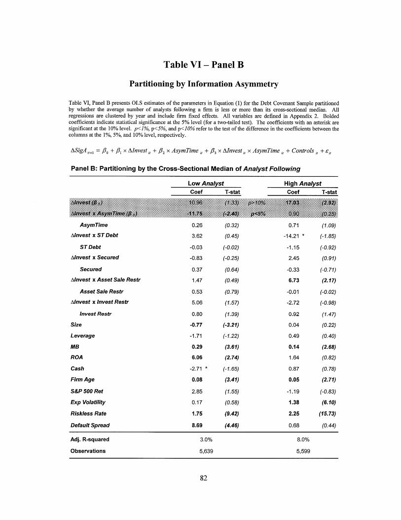
To test H2, I partition the sample by cross-sectional sample medians of each of the three

proxies for the richness of the firm's information environment. The first proxy is the average

daily closing bid-ask spread over the past year (Bid-Ask). The second proxy is the average

number of analysts that followed the firm in the past year (Analyst). The third proxy is the

adjusted probability of informed trading score (AdjPIN Score).2 3 I expect that accounting

quality will play a larger role in mitigating risk shifting for firms with poor information

environment, i.e., for firms with high Bid-Ask, low Analyst, and high AdjPIN Score.

Specifically, I expect that f3 (Poor Info Envir) < 3 (Rich Info Envir) .

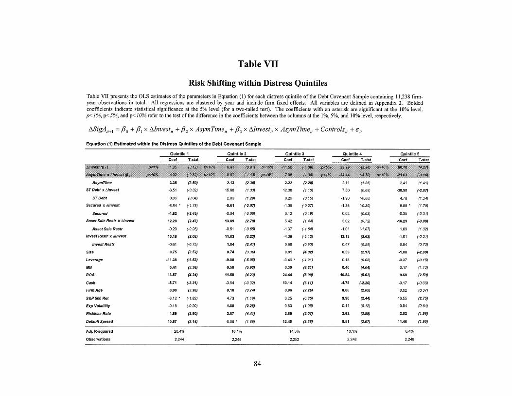
To test H3, I estimate Equation (1) for each of the Distress quintiles in order to examine

whether the level of distress risk affects risk shifting and the mitigating effect of accounting

quality. I expect the risk shifting effect (A1 >0) and the mitigating effect of asymmetric

timeliness (/3 < 0) will be stronger in higher distress risk quintiles. I do not use the distress

interaction term here because of a distinct possibility that the relation between risk shifting and

the level of distress may be non-monotonic.

To test H4 , I partition the top distress quintile by the cross-sectional median amount of

cash flow from operations in a given year scaled by lagged total assets. Specifically, I predict

that /3 (High CFO) < A (Low CFO).

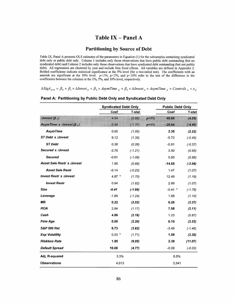
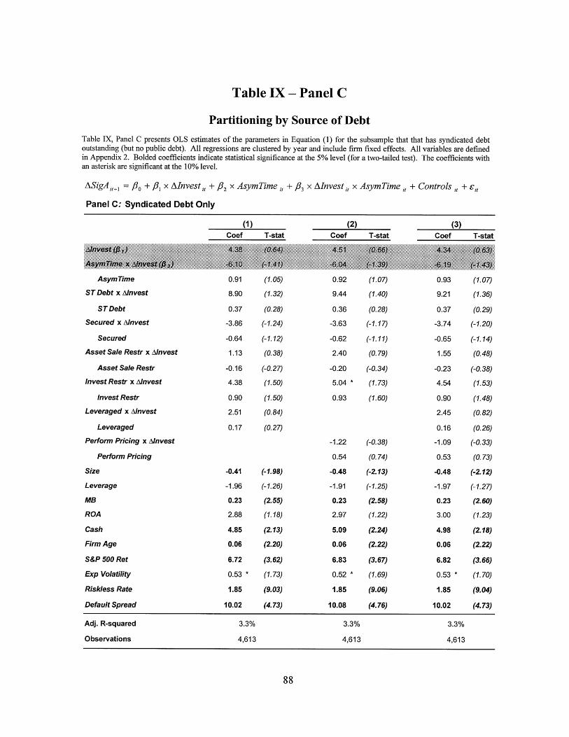
To test Hs, I partition the sample into two subsamples. The first subsample includes

those observations that only have public debt but no syndicated debt. The second subsample

23 1 obtained PIN estimates from Jefferson Duarte and Lance Young from the University of Washington. I use ameasure of asymmetric information AdjPIN from Duarte and Young (2009), which the authors argue is a bettermeasure of information asymmetry that the original PIN measure from Easley and O'Hara (2004).

includes those observations that only have syndicated but no public debt. I do not use the

observations that have both public and syndicated debt to test H5 since my goal is to try to

disentangle the effect of the source of debt on the relation between asymmetric timeliness and

risk shifting. I control for debt contract features that are present only in public or syndicated

debt. For the first subsample, I control for whether a firm has convertible debt (Convertible) or a

cross default provision in its debt contracts (Cross Default). For the second subsample, I add a

control for whether a firm has a leveraged syndicated loan (Leveraged) or a performance pricing

feature (floating spread over LIBOR) in its debt contract (Perform Pricing).

To test H6, I partition the sample into the pre-SOX and the post-SOX period. Since SOX

was adopted in late July of 2002, I divide the sample based on whether the fiscal year-end falls

before versus after July 31, 2002.24 I expect that accounting quality will have a larger effect after

the adoption of SOX, i.e., 63 (Pr e - SOX) < ,3 (Post - SOX).

One econometric concern that may affect the results is correlations among residuals in

Equation (1). While residuals estimated in models where the dependent variable is measured in

changes usually exhibit low correlation, I address a potential concern of correlations in the error

structure using an approach suggested by Petersen (2009). The residuals in Equation (1) are

estimated with firm fixed-effects and are clustered by year.25

Another concern is potential endogeneity. If decisions about the level of business risk are

made simultaneously with investment or accounting choices, the endogenous nature of this

relationship may bias the results. I argue that two factors can alleviate the endogeneity concern.

24 I also use the December 31, 2002 as a cutoff for robustness and the results remain qualitatively unchanged.25 I do not implement a two-dimensional clustering procedure (by year and by firm) due to the insufficient numberof observations in firm clusters. The results in Figure 5 of Peterson (2009) suggest that each cluster should have atleast 10 observations to allow for an estimation of the correlation structure without a large bias. While the sample inthe paper spans 12 years (from 1995 to 2006), each firm appears in the sample approximately 5 times (median = 4times). As a result, clustering by firm will not yield unbiased estimates.

First, all three main firm characteristics are measured in different time periods. As Figure 2

illustrates, accounting quality is measured prior to t = 0, investment is measured in the period

between t = 0 and t = 1, and changes in asset volatility are measured in the period between t = 1

and t = 2. I argue that regressing one-period-ahead volatility changes on lagged investment and

accounting quality is a way to reduce endogeneity since a significant part of accounting and

investment choices in the firm's financial statements is fixed by prior investment and production

decisions. This argument is similar to the one advanced by Frankel and Litov (2009). Second,

using changes instead of levels for asset volatility and investment intensity ensures that these

variables are not sticky, which also helps reduce the endogeneity concern.

3.2. Measures of asset volatility and distress

To estimate the firm-specific asset value volatility (SigA) and distress risk (Distress), I

use a technique similar to that used in a number of recent papers (e.g., Hillegeist et al., 2004,

Vassalou and Xing, 2004; Campbell et al., 2008) and solve a system of two non-linear equations.

The first equation (the BSM equation) is based on the Merton (1974) model, which expresses the

value of the firm's equity as a call option on the firm's assets using the Black-Scholes-Merton

option-pricing framework.26 The second equation represents the relation between the volatility

of equity and asset returns derived from Ito's lemma:27

Equation 1: the Black-Scholes-Merton equation for the value of equity with dividends:

VE = VA Xe- N(d) - TL x e-r TN(d 2) + VA x (1-e - ) (2)

Equation 2: the optimal hedge equation with dividends:

26 Variable descriptions and other details on the model are provided in Appendix 3.27 The derivation of the optimal hedge equation is presented in Appendix 4.

SigE = [e-N(d) + (1-e )]xA x SigA (3)VE

The system is simultaneously solved for the unobservable variables V and SigA, the

market value of assets and asset volatility, respectively. I estimate Distress as the probability

that the firm's asset value falls below the book value of its total liabilities (TL) at debt maturity 28

(after T years from time t = 0) assuming that the firm's asset value (continuous rate of growth in

assets) is log-normally (normally) distributed.29 Formally,

Distress N Iln(VA/TL)+ [p - - (SigA2 /2)] TDistress = N Sig -x V Y (4)

SigAx

where p is estimated as i = In VA, , + - In VA,_ + 0.5SigA2

3.3. Measure of accounting quality

I use a firm-year measure of asymmetric timeliness, C-Score, developed by Khan and

Watts (2009). The authors provide evidence that C-Score captures both cross-sectional and time-

series variation in the level of firm's asymmetric timeliness and can predict a firm's asymmetric

timeliness for up to three years in the future. This firm-year measure is estimated by treating the

asymmetric timeliness coefficient from Basu (1997) as a linear function of time-varying firm-

specific characteristics that are predicted to vary with the level of conservatism (size, market-to-

book, and leverage).

AsymTime,, = C_ Score, = , = Alt + 2,Size,, + A,M/B,, + 4,Lev,, (5)

The firm-specific time-varying coefficients (2 , withj = 1 to 4) are estimated as follows:

28 I use the procedure proposed by Barclay and Smith (1995-a) to estimated the expected time to maturity (T). Thedetails of this procedure are explained in Appendix 3.29 Strictly speaking, Distress is not an actual default probability since it does not correspond to the true defaultprobability in large samples. However, since this measure is a monotonic non-linear transformation of a true defaultprobability, it should produce similar distress rankings.

NI, = f, + 2,D, + R, (pI,, + ,uSize,, + jp,MB,, + p 4tLev, )+(6)

D,,R,, (+,Size,, + 3Size, + ,MB,, + 4tLev,, )+ E,

This measure of accounting quality is based on the notion of the differential verifiability

required for the recognition of accounting gains and losses developed by Basu (1997). Positive

returns proxy for good news and negative returns proxy for bad news.30 By allowing the

sensitivity of net income to vary for the subsamples of positive and negative returns (i.e., news),

the 34 coefficient captures the level of asymmetric timeliness that is present in the financial

statements. By incorporating both cross-sectional and time-series variation in size, market-to-

book, and leverage, 34 captures the firm-year-specific level of asymmetric timeliness.

I follow the procedure described in Khan and Watts (2009) to estimate AsymTime.

Specifically, I eliminate observations with missing data for any of the variables used in Equation

(1) and also with negative book value of equity or total assets. Returns are calculated by

cumulating monthly returns backwards starting from the third month after the fiscal year-end.

Equation (6) is then estimated for each year and cross-section-specific X-coefficients are

substituted in Equation (5) together with firm-specific measures of Size, MB, and Lev to calculate

AsymTime. The estimates are ranked into deciles by fiscal year and scaled to range from 0 to 1.31

30 The Basu measure takes the stock price as exogenous and thus implicitly assumes that the market is efficient.31 1 also estimate this model using a rolling panel consisting of all firm-year observations in each 3-digit SIC code inthe current and the four prior years. The two estimation techniques yield qualitatively similar empirical results.

4. Sample and Descriptive Statistics

I use several different data sources to construct a dataset combining contract-specific

information on public and private debt issues with various accounting and financial data. I use

the Mergent Fixed Investment Securities Database (FISD) to obtain a sample of public debt

issuances (the Public Debt Sample). I use the Securities Data Corporation's (SDC) database to

obtain a sample of syndicated loans (the Syndicated Loan Sample).

Combining the two samples and aggregating the data at the firm-year level creates the

main sample used in the study (the Debt Covenant Sample), which consists of 11,238 firm-years

from 2,344 unique firms and incorporates contract-specific information from 7,680 public and

private debt issues. I also use data from CRPS and Compustat to obtain descriptive statistics of

all Compustat firms for comparison purposes (the Compustat Sample) and to obtain various

firm-specific data items. Each one of the five above-mentioned samples is described below.

4.1. Public Debt Sample

I use the Mergent Fixed Investment Securities Database (FISD) to obtain a sample of

public debt issuances between January 1995 and December 2005. The FISD contains

information on terms and conditions of bond issues (on over 200,000 borrowers) as well as

information on exchange transactions reported by property and life insurers, and state insurance

departments. I follow prior research to construct a sample of firms that have information on

contractual features of public debt (e.g., Billett et al., 2007; Nikolaev, 2007). The sample

excludes foreign bonds, bonds denominated in foreign currency, bond issues by financial firms

(SIC codes 6000 to 6999), and U.S. government bonds. I then select debt issues from 1995 until

2005 that have covenant data available.

Initially, the Public Debt Sample contains 8,800 debt issues from 3,416 firms (Table I,

Panel A). Panel B provides descriptive statistics for the Public Debt Sample on a deal level and

before it is merged to Compustat. The mean (median) amount of a debt issuance is $300 ($200)

million and the mean (median) years-to-maturity is 11.8 (9.7) years, indicating that public debt

tends to be fairly long-term (75% of the issues have maturity of over 6 years). The vast majority

of issues are senior (95%), which is consistent with Billett et al. (2007) findings that the FISD

contains very few junior debt issues, and 30% of all issues are secured.

I collect information on four different types of bond covenants. The majority of debt

issues have M&A restrictions (93%) and asset sale restrictions (94%). However, very few debt

contracts have built-in investment restrictions (3%). This evidence is similar to prior findings

(Billett et al., 2007; Beatty et al., 2007) and suggests that the costs of over-restricting firm

investment choices outweighs the benefits of reduced wealth transfers. In addition,

approximately two-thirds of debt issues (64%) contain cross-default provisions.

I aggregate the FISD data at the firm-level and match it to Compustat. For each match, I

verify the company name and industry membership (based on the 3-digit SIC code). The

resulting sample consists of 12,489 firm-years from 2,034 firms that have at least one public debt

issue outstanding; 5,761 issues can be merged to Compustat (Table I, Panel A). Table I, Panel C

provides descriptive statistics for the Public Debt Sample on a firm-year level and after merging

it to Compustat. The mean (median) amount of public debt outstanding per firm-year is $683

($260) million. The mean (median) of the average face-value-weighted time to maturity is 8.6

(6.7) years. Almost 30% of firm-years have a public deal originating in that year. The statistics

on other features are similar to those in Panel B.

4.2. Syndicated Loan Sample

I use the Securities Data Corporation's (SDC) database to obtain a sample of syndicated

loans issued between January 1995 and December 2005. The sample excludes loans made to

non-U.S.-based companies, loans denominated in foreign currency, and loans made to financial

firms (SIC codes 6000 to 6999). I then select syndicated loans issued from 1995 until 2005 that

have covenant data available. Initially, the Syndicated Loan Sample contains 8,099 syndicated

loan deals and 4,411 individual firms (Table I, Panel A). Panel B provides descriptive statistics

for the Syndicated Loan Sample on a deal level and before merging it to Compustat.

The mean (median) amount of loan is $368 ($150) million and the mean and the median

loan maturity is 4.1 years, which is about two times shorter that the maturity of an average public

debt issue. In fact, 75% of the issues have the maturity of less than 5 years. Virtually all

syndicated loans are senior, consistent with Yago and McCarthy (2004). Secured loans

constitute 57% of the sample, while 55% of the loans are leveraged. Approximately half of the

loans have M&A restrictions (51%) and asset sale restrictions (49%). Restrictions on capital

expenditures are observed in 39% of the loans, which is close to the ratios observed in prior

research (Beatty et al, 2007; Nini et al., 2009). Similarly to the statistics in Roberts and Sufi

(2009), most loans (79%) have performance pricing features (floating spread over LIBOR).

I aggregate the SDC data at the firm-level and match it to Compustat. For each match, I

verify the company name and industry membership (based on the 3-digit SIC code). The

resulting sample consists of 12,788 firm-years from 2,638 firms that have at least one syndicated

loan outstanding; 5,511 loans can be merged to Compustat data (see Table I, Panel A). Table I,

Panel C provides descriptive statistics for the Syndicated Loan Sample on a firm-year level and

after merging it to Compustat. The mean (median) amount of syndicated debt outstanding per

firm-year is $599 ($220) million. The mean (median) of the average face-value-weighted time to

maturity is 2.7 (2.5) years. A third of firm-years have a syndicated loan deal that originated in

that year (Deal Year = 0.33). The descriptive statistics on other features are similar to those

shown in Panel B.

4.3. Debt Covenant Sample

To obtain a sample of firms that have either public or syndicated debt outstanding and

have details on debt covenants, I merge the Public Debt Sample with the Syndicated Loan

Sample. The resulting Debt Covenant Sample spans 12 years (from 1995 until 2006), 32 contains

20,274 firm-year observations from 3,573 firms, and covers 11,272 debt issuances, either public

or syndicated (see Table I, Part A). The requirement that the sample has non-missing data for

the main variables (asset volatility, investment intensity, and distress risk) and the control

variables reduces the sample to 11,238 firm-year observations from 2,344 firms. From these,

6,625 observations from 1,291 firms have public debt outstanding, 7,897 observations from

1,861 firms have a syndicated loan outstanding, and 3,284 observations from 808 firms have

both (see Table I, Panel A).

To test hypotheses that are conditional on the level of distress (H3 and H4), I rank all

observations in the Debt Covenant Sample into Distress quintiles within each fiscal year. The

resulting top distress quintile, for example, consists of 2,246 observations from 1,183 firms;

1,432 observations from 710 firms have public debt; 1,486 observations from 863 firms have

private debt; and 672 observations from 375 firms have both.

32 The Debt Covenant Sample covers an extra year that is not covered by either the Public Debt Sample or theSyndicated Loan Sample (2006). This happens because I include 2006 observations with non-missing data for themain variables that have outstanding public or syndicated debt.

The sample composition is presented in Table II. Panel A shows the observations

frequency breakdown by year. Relative to the Compustat comparison group, a disproportionate

fraction of observations in the Debt Covenant Sample and the top distress quintile have fiscal

years ending in 2002 - 2006, while years 1995 - 1997 are underrepresented. Panel B of Table II

presents the industry composition based on the Fama and French (1997) industry classification

(12 industry groups).33 Manufacturing, energy, telecommunications and wholesale and retail

industries are overrepresented while business equipment and healthcare industries are

underrepresented in the Debt Covenant Sample relative to the Compustat Sample (see below).

4.4. Compustat Sample

The Compustat Sample is retrieved from the 2008 Compustat annual primary, secondary,

tertiary and full-coverage research files and consists of all available firm-year observations from

U.S.-based non-financial firms that have fiscal year ending between January 1995 and December

2006. I require that all observations have non-missing SIC code, cash (data item 1), net income

(data item 172), and operating cash flow (data item 308). I also require that all observations

have positive total assets (data item 6) in the current and the previous years, total liabilities (data

item 181), net sales (data item 12), common share price (data item 199), and common shares

outstanding (data item 25). In addition, I remove the observations with negative book value of

equity (data item 60) to make the Compustat Sample comparable to the Debt Covenant Sample.

Observations with negative book values are excluded from the calculation of AsymTime are not

in the Debt Covenant Sample. The resulting sample has 54,388 firm-years from 9,048 firms.

33 Industry group definitions are available from Kenneth R. French's website athttp://mba.tuck.dartmouth.edu/pages/facultv/ken.french/Data Librarv/changes ind.html

4.5. Descriptive statistics

Table III, Panel A presents the comparison between the statistics for the Debt Covenant

Sample and the Compustat Sample. I winsorize all calculated variables (Firm Age, MB,

Leverage, ROA, CFO, and Cash) at 1% and 99% to control for non-linearities and outliers. 34 An

average firm in the debt covenant sample is over two times larger (based on Ve, TA, or Sales),

more profitable (based on CFO, ROA, and the incidence of losses), and older (20.3 vs. 17.5

years) than an average firm on Compustat. The former is also more leveraged (0.61 vs. 0.48)

and has two times less cash as a fraction of its total assets (0.11 vs. 0.22). The difference in cash

holdings may be due to the fact that an average firm in the Debt Covenant Sample has better

investment opportunities that an average firm in the Compustat Sample.

Table III, Panels B and C present descriptive statistics for the Debt Covenants Sample

and the top distress quintile, respectively. An average distressed firm is smaller than its

counterpart in the Debt Covenant Sample as measured both by market-based (Va and Ve) or

accounting-based measures (Sales, TA, and BVE). It has lower MB (1.48 vs. 2.68), higher

Leverage (0.71 vs. 0.61), and less short-term debt (St Debt is 0.11 vs. 0.16). An averaged

distress firm is riskier as evidenced by higher expected default probability (Distress is 0.30 vs.

0.07) over the next 3 years, higher asset volatility (SigA is 0.39 vs. 0.27) and equity volatility

(SigE is 0.70 vs. 0.45). It has performed worse economically as shown by lower prior 12-month

return (Ret is -0.22 vs. 0.18), operating cash flow (CFO is 0.04 vs. 0.09), return on assets (ROA

is -0.05 vs. 0.02), and higher incidence of losses (Loss is 0.55 vs. 0.25).

Revealingly, an average distressed firm exhibits approximately the same level of

accounting quality as healthy firms (AsymTime is 0.13 versus 0.14). This observation suggests

that firms, on average, do not alter their accounting choices significantly as economic conditions

34 All results are robust to various winsorizing cutoffs as well as to truncation.

deteriorate. Investment intensity (Invest) is the same for both healthy and distressed firms (0.14),

suggesting that firms try to follow their long-term investment strategy even in distress.

Distressed firms are also younger (Firm Age is 16.2 vs. 20.3), have lower analyst following

(Analyst is 6.3 vs. 8.3) and higher bid-ask spread (Bid-Ask is 3% vs. 2%).

Most observations in the Debt Covenant Sample are financially healthy firms as indicated

by a low probability of default (for the 75% of observations the cumulative probability of

default, Distress, over the next 3.2 years is less than 4%). This cutoff is roughly comparable to

the cumulative default rate on BBB-rated (investment grade) corporate bonds between 1971 and

2004 (Altman and Hotchkiss, 2006, p. 174). Most firms in the top distress quintile have a high

probability of default (for 75% of the observations, the cumulative probability of default over the

next 3.5 years is 30%). This cutoff is roughly comparable to the cumulative default rate on BB-

rated (junk) corporate bonds. The mean value of Distress in the top distress quintile (30%) is

reasonably close to the cumulative default rate on CCC-rated corporate bonds. Overall, firms in

the top distress quintile exhibit characteristics typical of firms in financial distress.

5. Empirical Results

5.1. Univariate results

Table IV reports pairwise correlations among the measures of asset volatility, investment

intensity, distress, accounting quality, and firm-specific controls for the Debt Covenant Sample

(Panel A) and the top distress quintile (Panel B). The upper right-hand portion of each panel

displays the Pearson product-moment correlations, and the lower left-hand portion displays the

Spearman rank-order correlations.

The correlations reveal that the one-period-ahead change in asset volatility (ASigA) is

positively correlated with the change in investment intensity (Alnvest) and distress (Distress) for

both the Debt Covenant Sample and the top distress quintile. This evidence is consistent with

the expectation that asset riskiness increases in response to new investments. The change in

investment intensity is negatively correlated with the level of distress, suggesting that distressed

firms tend to invest less than healthy firms, either due to lack of resources and investment

opportunities, or because of contractual restrictions.

5.2. Main results (H)

Table V presents the results of testing H1 for the Debt Covenant Sample using Equation

(1), both with and without ST Debt, Secured, Asset Sale Restr, and Invest Restr and their

interactions with Alnvest.35 The coefficients on Alnvest (A3) and Alnvest x AccQ (A) are of

particular importance. A positive A indicates that the change in investment intensity is

positively associated with the change in asset volatility. A negative A suggests that accounting

35 The only difference across the six different specifications of Equation (1) is the inclusion of the four contractualcontrol variables (ST Debt, Secured, Asset Sale Restr, and Invest Restr) and their interactions with Alnvest. Column(1) presents the results without including any of the four controls. Columns (2) - (5) include one control (and itsinteraction with Alnvest) at a time while Column (6) includes all four controls (and their interactions with Alnvest).

quality mitigates risk shifting. Since AsymTime is a decile measure scaled from 0 to 1, 834 can

be interpreted as the effect moving from the lowest decile of accounting quality to the highest

has on risk shifting.

The fl coefficient is positive and significant at the 5% level (for a two-tailed test) in all

six specifications. This evidence is similar to that of Eisdorfer (2008) and is indicative of risk-

shifting behavior among distressed firms. The 63 coefficient is negative and significant at the

5% level (for a two-tailed test) in all six specifications. The absolute value ofI 3 relative to the

absolute value of A3 is approximately 0.6 (= 10.13 / 16.73), indicating that moving from the

lowest accounting quality decile to the highest one can reduce the sensitivity of risk changes to

new investments by about 60%. These results are robust to including the controls for the

proportion of short-term debt in the capital structure (ST Debt), for the presence of secured debt

(Secured) as well as for asset sale (Asset Sale Restr) and investment (Invest Restr) restrictions.

5.3. Partitioning by the richness of information environment (H2)

Results shown in Table VI provide strong evidence consistent with the prediction that the

mitigating effect of accounting quality on risk shifting is stronger when the firm's information

environment is poor. Partitioning the Debt Covenant Sample by any of the three proxies for

information environment yields consistent results. Accounting quality has a stronger effect on

risk shifting when the average daily bid-ask spread is high, the analyst following is low, and the

AdjPin Score is high. Formally, 3 is statistically different for the subsamples in each of the

three tests (at least at the 5% level) suggesting that the effects of high accounting quality increase

as the firm's information environment deteriorates.

5.4. Partitioning by the level of distress risk (H3)

Table VII presents the results of testing H3 within all distress quintiles. Risk shifting

effects (ll) and accounting quality effects (834) are significant at the 5% level only in the two

top distress quintiles. Neither coefficient is significant in the three lowest distress quintiles. The

test for the difference in coefficients reveals that A, and 83 in the 5th quintile are not statistically

different from their counterparts in the 4th quintile. However, A and 3 in the 5th quintile are

different from those in the 1st quintile (at the 1% and 10% levels, respectively) and / and /3 in

the 4th quintile are different from those in the 3rd quintiles (at the 5% and 1% level, respectively).

Estimating Equation (1) for the first 3 quintiles (1st - 3 rd pooled) versus the top 2 quintiles

(4th and 5th pooled) reveals that both 1 and f3 are different for the two subsamples (at the 1%

level each). This result is consistent with the expectation that risk shifting is stronger when the

level of distress is higher. Interestingly, the adjusted R-squared decreases from 20.4% for the

healthiest firm-years to 6.4% in the most distressed firm-years.

The significant coefficient on ST Debt suggest that increasing the proportion of short-

term debt in the capital structure by one standard deviation causes an 18% drop in risk shifting (=

0.24 x 38.90 / 51.07). The coefficient on Asset Sale Restr is also statistically significant and its

magnitude suggests that the presence of this covenant in one of the firm's debt agreements

causes a 32% drop in risk shifting (= 16.29 / 50.70). The coefficient on Secured is statistically

significant at the 10% level, but has a positive sign. It appears that firms with secured debt are

more likely to engage in risk shifting than firms without secured debt.36 The coefficient on

Invest Restr has the expected minus sign, but it is statistically insignificant. 37

5.5. Partitioning by the availability of cash (H4)

Table VIII shows the results of testing H4. The evidence seems to suggest that when cash

flow from operations is relatively high among distressed firms, accounting quality has a

mitigating effect on risk shifting, while if the cash flow from operations is low, it does not. The

value of 63 relative to the value of A is approximately two times higher, which suggests that

the effect of accounting quality on risk shifting in firms with high cash flow is double that in

firms with low cash flow. However, the test of the difference in the coefficients between the two

subsamples reveals that neither one is significantly different from its counterpart (p-value > 10%

in both cases). Thus, this test is inconclusive.

5.6. Partitioning by the source of debt (Hs)

Table IX presents the results from testing H5 by running the regression separately for

subsamples of the Debt Covenant Sample partitioned by the source of debt (public debt only

versus syndicated debt only). The evidence of risk shifting and the mitigating role of accounting

quality is statistically significant only in the Public Debt Sample. The relative magnitude of /3

and p suggests that risk shifting is more than two times lower for firms in the top accounting

quality decile than for their counterparts in the bottom accounting quality decile (28.64 / 49.65).

36 Once possible explanation to this observation may be the fact that secured creditors worry less about their debtinvestment ex post and, as a result, do not exert as much effort into monitoring and disciplining managers.37 Nini et al. (2009) provide evidence that capital expenditures restrictions constrain firm investment. However, asthe authors note, "capital expenditures ... are commonly set as s nominal dollar amount for a given year".Constraining the level of allowed capital expenditures says nothing about the constraining the level or risk of theseexpenditures. That is, a distressed firm with a capital expenditure restriction in place may still chose to invest theallowed amount into suboptimally risky assets.

In addition, A3 and f3 are statistically different from their counterparts in the two subsamples at

the 1% confidence level. This evidence suggest that accounting quality is an important

mechanism for bondholders that lowers the agency cost of debt, while it is less useful to private

debtholders due to their access to additional information channels unavailable to bondholders.

Panels B and C repeat the analysis for each subsample while introducing two pairs of

contractual features that are available only for the corresponding subsamples: a) the presence of a

convertibility option or a cross default provision in public debt (Convertible and Cross Default);

and b) the leveraged loan status and performance pricing features in syndicated debt (Leveraged

and Perform Pricing). The presence of convertible debt has a significant influence on the

reduction of risk shifting, although its effects (,3 = -10.80) are not as strong as those of

accounting quality (3, = -33.54). The presence of cross-default provisions is also significant,

but the sign of the coefficient is opposite from what I expected. The presence of leveraged loans

or of performance pricing features in syndicated debt does not appear significant.

5.7. Partitioning by the passage of SOX (H6)

The results from testing H6 are shown in Table X. The A coefficient is statistically

significant in the pre-SOX period, while it is not statistically significant in the post-SOX period.

The magnitude of/3 is higher in the post-SOX period. Both results are consistent with the

expectations that the adoption of SOX decreased corporate risk taking as well as made

accounting information more dependable and efficient for debt contracting purposes. Formally,

the difference between the two pairs of coefficients is not significant at conventional confidence

levels (p-value > 10% in both cases). Thus, the results of the test are inconclusive and it is

difficult to make any inferences from this test.

6. Robustness Tests

6.1. Using ASigE instead of ASigA

To address the concern regarding the difficulty of obtaining accurate estimates of asset

volatility, I use the change in the firm's one-period-ahead equity volatility, ASigE, as the

dependent variable instead of the one-period-ahead change in asset volatility, ASigA. If a firm

engages in risk-increasing activities, it will likely have volatile returns to capital (John et al.

2008). I expect that such behavior will eventually be reflected in the riskiness of the firm's

equity after controlling for the proportion of debt in the capital structure. I estimate equity

volatility (SigE) by using daily equity returns for the 252 trading days. The model below uses

ASigE instead of ASigA as the dependent variable.

ASigE1,, = 8 + fl x Alnvest,, + 82 x AccQ,, + px AJnvesti, x AccQ,, + Controls,, + c,, (7)

All other variables are identical to those in Equation (1). The results from using this

model are presented in Table XI, Panel A and are consistent with those in Table V. One

noticeable difference is that adjusted R-squared for the equity-volatility model are significantly

higher for the top two distressed quintiles (17.1% vs. 9.6% and 14.3% vs. 5.1% for the 4th and 5th

quintiles, respectively). This observation is consistent with the expectation that estimated asset

volatility of distressed firms may be considerably noisy.

6.2. Using an alternative measure of investment

I use an alternative proxy for investment by adding R&D to capital expenditures when

calculating investment intensity (Invest), similar to Verdi (2006). For the purpose of this

robustness test, I set all missing R&D observations (data item 46) equal to zero. All other model

specifications remain the same as in Equation (1). The results from this robustness test are

shown in Table XI, Panel B and are consistent with those in Table V.

6.3. Using leverage instead of distress risk

I use the degree of leverage instead of the level of distress risk to proxy for the amount of

benefits risk shifting provides to shareholders (e.g., Green and Talmor, 1986). I partition the

Debt Covenant Sample into leverage quintiles by year in the same way that I partition the sample

into distress quintiles in the main specifications. The results of estimating Equation (1) for

leverage quintiles are shown in Table XI, Panel C and are consistent with those in Table VII.

6.4. Partitioning by lease intensity

Sharpe and Nguyen (1995) note that leasing instead of buying equipment can provide

creditors, i.e., lessors, with more security and higher priority in bankruptcy, thus mitigating

agency problems that result from information asymmetries between the firm and capital

providers. In order to rule out the possibility that higher risk shifting activities of firms with poor

accounting quality are associated with their choices of leasing versus buying, I test whether the

effect of asymmetric timeliness on risk shifting depends on the level of lease intensity.

The results from partitioning the Debt Covenant Sample by cross-sectional medians of

lease intensity are shown in Table XI, Panel D. The A coefficient is significant in both

subsamples although the size of /3 relative to that of /, is about two times higher for the high

lease intensity subsamples (81.8% vs. 41.1%) indicating that accounting quality matters more for

firms that use leases more extensively. This result is consistent with the evidence presented in

Beatty et al. (2008) that firms with poor accounting quality are more likely to lease than to buy.38

6.5. Other robustness checks

I also subject the data to a battery of other sensitivity tests to ensure the stability of the

results. I use a number of alternative measures for size, leverage, profitability, expected market

volatility, and overall economy health. I also follow the procedure used by Eisdorfer (2008) and

exclude firm-years with significant new issues of equity or debt (more than 5% of total assets)

from the sample to address the concern that observed changes in volatility may be mechanically

driven by changes in the firm capital structure unrelated to the market value of assets. The

results of these tests are generally consistent with the main findings in this study.

38 Beatty et al. (2008) are interested in a different dimension of accounting quality. Namely, they proxy for theoverall accrual quality by using absolute value of current accruals.

7. Conclusion

This study examines the effect of accounting quality on risk shifting. I argue that

accounting quality helps mitigate risk shifting by aiding debtholders in monitoring and

disciplining firm's investment decisions. I predict that high accounting quality is associated with

lower changes in asset volatility in response to new investments and interpret such evidence as

an indication of lower risk shifting. I also test for whether the effect of accounting quality on

risk shifting differs depending on cross-sectional and time-series characteristics. I expect that

this effect will be more pronounced for firms with poor information environment, high distress

risk, and operating cash flows, and for observations in the post-SOX period. I also expect that

this effect will differ depending on the source of firm's debt. I use asymmetric timeliness in

recognition of bad versus good news as a dimension of accounting quality that is of a first-order

importance to debtholders.

The results are consistent with the expectations. Firms in the top accounting quality

decile exhibit significantly less risk shifting than firms in the bottom decile. The accounting

quality effects are significantly stronger for firms with poor information environment, high

distress risk, and with public debt in the capital structure. While there is some evidence that

accounting quality is more important in mitigating risk shifting for firm-years with high

operating cash flows and after the adoption of SOX, the difference is not statistically significant

at conventional confidence levels. The results are robust to using different sample modifications,

alternative measures of investment and distress, and to the inclusion of various control variables.

This study contributes to the accounting literature that examines the effects of accounting

quality on the severity of debt-equity agency conflicts (e.g., Biddle et al., 2008; Louis et al.,

2009). The results in this study strengthen the evidence provided by Zhang (2008) that both

lenders and borrowers benefit from asymmetric timeliness ex ante. I provide evidence

suggesting that borrowers with higher asymmetric timeliness behave ex post in a way that lowers

debt agency costs, which gives an explanation to why these borrowers are rewarded with a lower

cost of debt ex ante. This study also contributes to the growing literature in finance that

examines the role of covenants on the interaction of firms with their debt capital providers (e.g.,

Chava and Roberts, 2008; Roberts and Sufi, 2008; Nini et al, 2009-b) by proving evidence

suggesting that accounting quality affects the efficiency of this relationship.

This study can be extended along several avenues. First, an international setting can be

used to verify the claim made by Biddle and Hillary (2006) that the usefulness of accounting

quality for mitigating debt-equity agency conflicts is stronger in equity-dominated economies

than in debt-dominated ones. Second, the usefulness of other dimensions of accounting quality

for decreasing risk shifting can be examined, such as transparency, for example. Third,

researchers can examine whether accounting quality and other corporate governance mechanisms

complement or substitute each other in reducing risk shifting.

References

Ahmed, A., Duellman, S., 2007. Evidence on the role of accounting conservatism in monitoringmanager's Investment Decisions. Working paper, Texas A&M University and StateUniversity of NY at Binghamton.

Altman, E., 1968. Financial ratios, discriminant analysis and the prediction of corporatebankruptcy. Journal of Finance 23, 589-609.

Altman, E., Hotchkiss, E., 2006. Corporate financial distress and bankruptcy, 3 rd edition. JohnWiley & Sons, Inc.

Anantharaman, D., 2009. Do disclosure standards affect risk-taking in the banking industry? Across-country study. Working paper, Columbia University.

Angrade, G., Kaplan, S., 1998. How costly is financial (not economic) distress? Evidence fromhighly leveraged transactions that became distressed. Journal of Finance 53, 1443 - 1493.

Asquith, P., Beatty, A., Weber, J., 2005. Performance pricing in bank debt contracts. Journal ofAccounting and Economics 40, 101 - 128.

Ball, R., Kothari, S.P., Robin, A., 2000. The effect of international institutional factors onproperties of accounting earnings. Journal of Accounting and Economics 29, 1 - 51.

Ball, R., Shivakumar, L., 2005. Earnings quality in U.K. private firms: comparative lossrecognition timeliness. Journal of Accounting and Economics 39, 83 - 128.

Ball, R., Robin, A., Sadka, G., 2008. Is financial reporting shaped by equity markets or by debtmarkets? An international study of timeliness and conservatism. Review of AccountingStudies, forthcoming.

Barclay, M., Smith, C., 1995. The maturity structure of corporate debt. Journal of Finance 50,609 - 631.

Barclay, M., Smith, C., 1995. The priority structure of corporate liabilities. Journal of Finance50, 899 - 916.

Bargeron, L., Lehn, K., Zutter, C., 2009. Sarbanes-Oxley and corporate risk taking. Journal ofAccounting and Economics, forthcoming.

Barth, M., Landsman, W., Lang, M., 2008. International accounting standards and accountingquality. Journal of Accounting Research 46, 467 - 498.

Basu, S., 1997. The conservatism principle and the asymmetric timeliness of earnings. Journalof Accounting and Economics 24, 3 - 37.

Beatty, A., Liao, S., Weber, J., 2007. The role of accounting quality in reducing investmentinefficiency in the presence of private information and direct monitoring. Working paper,Ohio State University and Massachusetts Institute of Technology.

Beatty, A., Liao, S., Weber, J., 2008. Financial reporting quality, private information,monitoring and the lease-versus-buy decision. Working paper, Ohio State University andMassachusetts Institute of Technology.

Beatty, A., Weber, J., Yu, J., 2008. Conservatism and debt. Journal of Accounting andEconomics 45, 154 - 174.

Beatty, A., Ramesh, K., Weber, J., 2002. The importance of accounting changes in debtcontracts: The costs of flexibility in covenant calculations. Journal of Accounting andEconomics 33, 205 - 227.

Bhanot, K., Mello, A., 2006. Should corporate debt include a rating trigger? Journal ofFinancial Economics 79, p. 69 - 98.

Biddle, G., Hilary, G., Verdi, R., 2008. How does financial reporting quality improveinvestment efficiency? Working paper, University of Hong Kong, Hong Kong University ofScience and Technology, and Massachusetts Institute of Technology.

Biddle, G., Hilary, G., 2006. Accounting quality and firm-level capital investment. TheAccounting Review 81, 963 - 982.

Black, F., Scholes, M., 1973. The pricing of options and corporate liabilities. Journal ofPolitical Economy 81, 637 - 654.

Brealey, R., Myers, S., Allen, F., 2006. Principles of Corporate Finance, 8th edition.

Brown, K., Harlow, W., Starks, L., 1996. Of tournaments and temptations: An analysis ofmanagerial incentives in the mutual fund industry. Journal of Finance 51, 85 - 110.

Brown, S., Goetzmann, W., Park, J., 2001. Careers and survival: Competition and risk in thehedge fund and CTA industry. Journal of Finance 56, 1869 - 1886.

Bushman, R., Smith, A., 2001. Financial accounting information and corporate governance.Journal of Accounting and Economics 32, 237 - 333.

Bushman, R., Piotroski, J., Smith, A., 2006. Capital allocation and timely accountingrecognition of economic losses. Working paper, University of North Carolina and Universityof Chicago.

Campbell, J., Hilscher, J., Szilagyi, J., 2008. In search of distress risk. Journal of Finance,forthcoming.

Chava, S., Roberts, M., 2008. How does financing impact investment? The role of debtcovenants. Journal of Finance 63, 2085 - 2121.

Cohen, D., Dey, A., Lys, T., 2009. The Sarbanes Oxley Act of 2002: Implications ofcompensation contracts and managerial risk-taking. Working paper, New York University,University of Chicago and Northwestern University.

Crosbie, P., Bohn, J., 2001. Modeling default risk. KMV, LLC, San Francisco, CA.

De Franco, G., Vasvari, F., Wittenberg-Moerman, R., 2009. The information role of bondanalysts. Forthcoming, Journal of Accounting Research.

Dey, A., 2009. The chilling effect of Sarbanes-Oxley: A discussion of Sarbanes-Oxley andcorporate risk-taking. Journal of Accounting and Economics, forthcoming.

Diamond, D., 1991. Monitoring and reputation: The choice between bank loans and privatelyplaced debt. Journal of Political Economy 99, 689 - 721.

Dichev, I., Skinner, D., 2002. Large-sample evidence on the debt covenant hypothesis. Journalof Accounting Research 40, 1091 - 1123.

Drucker, S., Puri, M., 2009. On loan sales, loan contracting, and lending relationships. Reviewof Financial Studies, forthcoming.

Duarte, J., Young, L., 2009. Why is PIN priced? Journal of Financial Economics 91, p. 119 -138.

Easley, D., O'Hara, M., 2004. Information and the cost of capital. Journal of Finance 59, 1553- 1583.

Easton, P., Monahan, S., Vasvari, F., 2009. Initial evidence on the role of accounting earnings inthe bond market. Journal of Accounting Research 47, 721 - 766.

Easton, P., Nikolaev, V., van Lent, L., 2009. Price convexity, debt-related agency costs, timelyloss recognition. Working paper, University of Notre Dame, University of Chicago, andTilburg University.

Eckbo, B., Thorburn, 2003. Control benefits and CEO discipline in automatic bankruptcyauctions. Journal of Financial Economics 69, 227 - 258.

Eisdorfer, A., 2008. Empirical evidence of risk shifting in financially distressed firms. Journalof Finance 63, 609 - 637.

Fields, T., Lys, T., Vincent, L., 2001. Empirical research on accounting choice. Journal ofAccounting and Economics 31, 255 - 307.

Francis, J., LaFond, R., Olsson, P., Schipper, K., 2004. Cost of equity and earnings attributes.The Accounting Review 79, p. 967 - 1010.

Francis, J., Martin, X., 2008. Acquisition profitability and timely loss recognition. Workingpaper, University of Missouri - Columbia and Washington University in St. Louis.

Frankel, R., Litov, L., 2007. Financial accounting characteristics and debt covenants. Workingpaper, Washington University in St. Louis.

Franzen, L., Rodgers, K., Simin, T., 2007. Measuring distress risk: The effect of R&D intensity.Journal of Finance 62, 2931 - 2967.

Galai, D., Masulis, R., 1976. The option pricing model and the risk factor of stock. Journal ofFinancial Economics 3, 53 - 81.

Gavish, B., Kalay, A., 1983. On the asset substitution problem. Journal of Financial andQuantitative Analysis 18, 21 - 30.

Gigler, F., Kanodia, C., Sapra, H., Venugopalan, R., 2009. Accounting conservatism and theefficiency of debt contracts. Journal of Accounting Research 47, 767 - 797.

Givoly, D., Hayn, C., 2000. The changing time-series properties of earnings, cash flows andaccruals: Has financial reporting become more conservative? Journal of Accounting andEconomics 29, 287 - 320.

Graham, J., Harvey, C., Rajgopal, S., 2005. The economics implications of corporate financialreporting. Journal of Accounting and Economics 40, 3 - 73.

Green, C., 1984. Investment incentives, debt, and warrants. Journal of Financial Economics 13,115-136.

Green, R., Talmor, E., 1985. The structure and incentive effects of corporate tax liabilities.Journal of Finance 40, 1095 - 1114.

Green, R., Talmor, E., 1986. Asset substitution and the agency costs of debt financing. Journalof Banking and Finance 10, 391 - 399.

Guay, W., 2008. Conservative financial reporting, debt covenants, and the agency cost of debt.Journal of Accounting and Economics 45, 175 - 180.

Guay, W., Verrecchia, R., 2006. Discussion of an economic framework for conservativeaccounting and Bushman and Piotroski (2006). Journal of Accounting and Economics 42,149- 165.

Hillegeist, S., Keating, E., Cram, D., Lundstedt, K., 2004. Assessing the probability ofbankruptcy. Review of Accounting Studies 9, 5 - 34.

Hirshleifer, D., Thakor, A., 1992. Managerial conservatism, project choice and debt. Review ofFinancial Studies 5, 437 - 470.

Hubbard, R., 1998. Capital-market imperfections and investment. Journal of EconomicLiterature 36, 193 - 225.

Hu, H., 2009. Empty creditors and the crisis. The Wall Street Journal, April 9, 2009.

Jensen, M., Meckling, W., 1976. Theory of the firm: Managerial behavior, agency costs andownership structure. Journal of Financial Economics 3, 305 - 360.

Jensen, M., Smith, C., 1985. Stockholder, manager, and creditor interests: Applications ofagency theory. Recent Advances in Corporate Finance, edited by E. Altman and M.Subramanyam, Dow-Jones Irwin.

John, K., Litov, L., Yeung, B., 2008. Corporate governance and risk taking. Journal of Finance63, p 1679 - 1728.

Khan, M., Watts, R., 2009. Estimation and empirical properties of a firm-year measure ofconservatism. Journal of Accounting and Economics, forthcoming.

Kothari, S.P., Shu, S., Wysocki, P., 2009. Do managers withhold bad news? Journal ofAccounting Research 47, 241 - 276.

Kothari, S., Lys, T., Smith, C., Watts, R., 1988. Auditor liability and information disclosure.Journal of Accounting, Auditing, and Finance 3, 307 - 339.

LaFond, R., Watts, R., 2008. The information role of conservatism. The Accounting Review 83,447 - 478.

Lambert, R., Leuz, C., Verrecchia, R., 2007. Accounting information, disclosure, and the costsof capital. Journal of Accounting Research 45, 385 - 426.

Louis, H., Sun, A., Urcan, 0., 2009. Value of cash holdings and accounting conservatism.Working paper, Pennsylvania State University and London Business School.

Lys, T., Watts, R., 1994. Lawsuits against auditors. Journal of Accounting Research 32, 65 -93.

Mallor, J., Barnes, A., Bowers, T., Phillips, M., Langvardt, A., 2001. Business law and theregulatory environment: Concepts and cases, 11t edition. McGraw-Hill Higher Education.

McDaniel, M., 1986. Bondholders and corporate governance. Business Lawyer 41, p. 413 -460.

Mehran, H., 1995. Executive compensation structure, ownership, and firm performance. Journalof Financial Economics 38, 163 - 184.

Merton, R., 1974. On the pricing of corporate debt: The risks structure of interest rates. Journalof Finance 29, 449 - 470.

Morck, R., Shleifer, A., Vishny, R., 1988. Management ownership and corporate performance:An empirical analysis. Journal of Financial Economics 20, 293 - 315.

Myers, S., 1977. Determinants of corporate borrowing. Journal of Financial Economics 5, 147 -175.

Myers, 2001. Capital structure. Journal of Economic Perspectives 15, 81 - 102.

Nikolaev, V., 2007. Debt covenants and accounting conservatism. Working paper, Universityof Chicago.

Nash, R., Netter, J., Poulsen, A., 2003. Determinants of contractual relations betweenshareholders and bondholders: Investment opportunities and restrictive covenants. Journal ofCorporate Finance 9, 201 - 232.

Nini, G., Smith, D., Sufi, A., 2009. Creditor control rights and firm investment policy. Journalof Financial Economics 92, 400 - 420.

Nini, G., Smith, D., Sufi, A., 2009. Creditor control rights, corporate governance, and firmvalue. Working paper, University of Pennsylvania, University of Virginia, and University ofChicago.

Ohlson, J., 1980. Financial ratios and the probabilistic prediction of bankruptcy. Journal ofAccounting Research 18, 109 - 131.

Parrino, R., Weisbach, M., 1999. Measuring investment distortions arising from stockholder-bondholder conflicts. Journal of Financial Economics 53, 3 - 42.

Petersen, M., 2009. Estimating standard errors in finance panel data sets: Comparingapproaches. Review of Financial Studies 22, 435 - 480.

Pratt, J., Stice, J., 1994. The effects of client characteristics on auditor litigation risk judgments,required audit evidence, and recommended audit fees. The Accounting Review 69, 639 -656.

Purnanandam, A., 2008. Financial distress and corporate risk management. Theory andevidence. Journal of Financial Economics 87, 706 - 739.

Rauh, J., 2009. Risk shifting versus risk management. Investment policy in corporate pensionplans. Review of Financial Studies 22, 2687 - 2733.

Roberts, M., Sufi, A., 2008. Control rights and capital structure: An empirical investigation.Journal of Finance 63, 2085 - 2121.

Roychowdhury, S., Watts, R., 2007. Asymmetric timeliness of earnings, market-to-book andconservatism in financial reporting. Journal of Accounting and Economics 44, 2 - 31.

Ryan, S., 2006. Identifying conditional conservatism. European Accounting Review 15, 511 -525.

Sharpe, S., Nguyen, H., 1995. Capital market imperfections and the incentive to lease. Journalof Financial Economics 39, 271 - 294.

Skinner, D., 1994. Why firms voluntarily disclose bad news. Journal of Accounting Research32, 38 - 60.

Skinner, D., 1997. Earnings disclosures and stockholder lawsuits. Journal of Accounting andEconomics 23, 249 - 282.

Smith, C., Warner, J., 1979. On financial contracting: An analysis of bond covenants. Journal ofFinancial Economics 7, 117 - 162.

Sunder, J., Sunder, S., Zhang, J., 2009. Balance sheet conservatism and debt contracting.Working paper, Northwestern University.

Vassalou, M., Xing, Y., 2004. Default risk in equity returns. Journal of Finance 59, 831 - 868.

Verde, M., 1999. Loan preserver: The value of covenants. Loan Products Special Report, FitchIBCA.

Watts, R., 2003. Conservatism in accounting, Part I: Explanation and implications. AccountingHorizons 17: 207 - 221.

Watts, R., 2006. What has the invisible hand achieved? Information for better capital marketsconference. London, Institute of Chartered Accountants in England and Wales.

Weiss, L., 1990. Bankruptcy resolution: Direct costs and violation of priority of claims. Journalof Financial Economics 27, p. 285-314.

Yago, G., McCarthy, D., 2004. The U.S. leveraged loan market: A primer. CA, USA: MilkenInstitute.

Zhang, J., 2008. The contracting benefits of accounting conservatism to lenders and borrowers.Journal of Accounting and Economics 45, 27 - 54.

Appendix 1: Examples of Risk Shifting

Panel A - Binomial Distribution Example (Hypothetical)

Firm A (Face Value of Debt = 100) Firm B (Face Value of Debt = 150)

Face Value of Debt

Up StateDown StateExpected Value

Debt Value / Face

Volatility

Volatilty Increase

Up StateDown StateExpected Value

Debt Value / Face

Volatility

A Expected Value% A Expected Value

100 Market ValuesProb Assets Debt Equity0.5 200 100 1000.5 100 100 0

150 100 50

100.0%

5 0 50

Market ValuesProb Assets Debt Equity0.5 205 100 1050.5 95 95 0

\ 150 97.5 52.5

97.5%

2.5 52.5

Face Value of Debt

Up StateDown StateExpected Value

Debt Value / Face =

Volatility

Volatilty Increase

Up StateDown StateExpected Value

Debt Value / Face =

150

Volatility

A Expected Value% A Expected Value

Market ValuesProb Assets Debt Equity0.5 250 150 1000.5 50 50 0

150 100 50

66.7%

100 50 50

Market ValuesProb Assets Debt Equity0.5 260 150 1100.5 40 40 0

150 95 55

63.3%

110 55 55

0.0 -5.0 5.00.0% 1 -5.0% 10.0%

0.0 -2.5 2.50.0% -2.5% 5.0%

Panel A presents a hypothetical example (with the binomial distribution of outcomes) of how changing the volatility of assets benefitsequityholders to the detriment of debtholders. This example demonstrates that the same (proportional) increase in asset volatilitycauses a higher increase in equity value for shareholders of a riskier firm. This happens due to the asymmetric nature of debt payoffsthat results in unequal sharing of the upside and the downside of increased risk by shareholders and debtholders.

The only two possible states of the world, the up state and the down state, are equally likely. There are two firms, Firm A and Firm B.Both firms have the same expected market value of assets, debt, and equity of 150, 100, and 50, respectively. However, Firm A is lessrisky than Firm B both because it has a lower volatility of its asset base (50 versus 100) and less debt (face value of 100 versus 150).At the beginning, Firm A is virtually safe because the value of its assets will be enough to repay all 100 of its debt in both states of theworld. As a result, Firm A's debt is trading at 100% of its face value. Firm B, on the other hand, will not be able to repay all 150 ofits debt in the down state because the value of assets in this scenario will only be 50. As a result, Firm B's debt is trading at 66.7% ofits face value (= 150 x 0.5 + 50 x 0.5).

Both firms have an option to engage in new risky projects and increase the volatility of their assets by 10% (relative to their respectiveinitial level of volatility). That is, Firm A can increase it asset volatility from 50 to 55 (= 50 x 1.1) while Firm B can increase itsvolatility from 100 to 110 (= 100 x 1.1). For simplicity, let us assume that new projects have symmetric payoffs in both up and downstates of the world, and, as a result, will not change the expected value of assets for both firms. In other words, the effect ofundertaking these additional projects will be an increase in asset volatility without any change in the expected value of assets. If wekeep the probabilities of the states of the world happening the same (at 50-50) and increase the volatility by 10% while leaving theexpected value of assets the same at 150, there is a unique solution to what the new value of asset will be in both states.

As can be seen in the bottom part of Panel A, an increased in asset volatility causes the debt to become more risky in both firms. FirmA now will not be able to fully repay its 100 worth of obligations in the down state since the market value of assets will only be 95.As a result, Firm A's debt is now trading at 97.5% (= 100 x 0.5 + 95 x 0.5). Firm B's debtholders also bear a loss in the value of debtsince they do not benefit from the higher asset value in the up state but they do receive less in the down state (40 instead of 50).Consequently, the value of their debt claims now drop from 66.7% of the face value to 63.3% (= 150 x 0.5 + 40 x 0.5).

Since the change in the expected value of assets does not change by design, any decreases in debt value due to increased riskiness willcause the value of equity to increase. As shown at the bottom of the panel, the expected value of Firm A's debt will decrease by 2.5 (97.5 - 100) and the value of its equity will increase by 2.5 (= 52.5 - 50). This corresponds to a 2.5% drop in the value of debt (= 2.5 /100) and to the 5.0% increase in the value of equity (= 2.5 / 50). The expected value of Firm B's debt will decrease by 5.0 (95 - 100)and the value of its equity will increase by 5 (55 - 50). This corresponds to a 5% drop in the value of debt (= 5 / 100) and to a 10%increase in the value of equity (= 5 / 50).

Appendix 1: Examples of Risk Shifting

Panel B - Continuous Distribution Example (Empirical)

Debt Covenant Sample Top Distress Quintile

Market Value of Assets (Va)Total Liabilities (TL)Wtd Debt Maturity (Wtd YTM)Asset Return Volatility (SigA)Riskless Rate (Rf)Dividend Rate (Div Rate)

Market Value of Equity (Ve)

Mean Firm Median Firm6,529 1,4122,633 562

3.18 3.3527.34% 21.76%

3.69% 4.55%-3.14% 1.99%

4,879 839

Mean Firm Median Firm2,232 5861,604 3863.49 3.65

38.93% 32.03%3.69% 4.49%

-0.45% 1.36%

1,051 257

Option Vega 1.98 0.23 10.08 2.13Full Sample vs. Distress Quintile (x 5.1) (x 9.1)

Elastisity Vega 0.01 0.01 0.37 0.27Full Sample vs. Distress Quintile (x 33.7) (x 43.8)

Panel B presents an example (with a continuous distribution of outcomes) illustrating that theeffect of increasing asset volatility on equity value increases in distress risk. Two pairs of firmsare compared: a "Mean Firm" from the Debt Covenant Sample and the top distress quintile, anda "Median Firm" from the same samples. The mean and median firms' characteristics are themeans and the medians of the corresponding samples.

The values for the market value of assets, total liabilities, weighted debt maturity, asset returnvolatility and the riskless rate are input into the Black-Scholes model. I calibrate the model byusing the dividend rate that makes the output (market value of equity) equal to the mean (ormedian) market value of equity that has been estimated as described in Appendix 3. OptionVega is the sensitivity of the equity value to changes in asset volatility. Elasticity Vega is therelative sensitivity of the value of equity to changes in asset volatility. Formally,

a Ve 8 Ve/ VeOption Vega = a A and Elasticity Vega =

aSigA aSigA/SigAOption Vega = 10 means that a mean firm from the top distress quintile will experience anincrease in the value of equity of $10 million for a 1% (absolute) change in asset volatility.Since the mean value of equity is $1,051 million, this increase corresponds to a 0.95% return onequity. Elasticity Vega = 0.37 means that a mean firm from the top distress quintile willexperience a 0.37% increase in equity for a 1% (relative) change in asset volatility. Since a 1%absolute change in asset volatility corresponds to approximately a 2.6% relative change (= 1% /39%) in equity value and thus correspond a 0.95% return on equity (= 2.6% x 0.37).

Option Vega and Elasticity Vega are correspondingly 5 and 34 times higher for the mean firm inthe top distress quintile than for the mean firm in the Debt Covenant Sample. Option Vega andElasticity Vega are correspondingly 9 and 44 times higher for the median firm in the top distressquintile than for the median firm in the Debt Covenant Sample.

Appendix 2: Variable Definitions

Dependent variablesSigA ,

ASigA t+,

SigE ,

ASigE+1

Measures ofInvest,

Alnvest,

AsymTime,

Firm-specific asset value volatility estimated using the Merton (1974)model (see Appendix 3 for details)The change in firm-specific asset return volatility in period t + 1, i.e.,SigA t+2-SigA t+lFirm-specific equity value volatility estimated using prior 90 trading days

The change in firm-specific asset return volatility in period t + 1, i.e.,SigE ,+2-SigE ,,+1

investment and accounting qualityInvestment intensity, capital expenditures scaled by beginning PPE, i.e.,Data128 / Data7The change in Invest, in period t, i.e., Invest,,, - Invest,Asymmetric timeliness measure from Khan and Watts (2009), C_Score

Partitioning variablesBid - Ask, Closing daily bid-ask spread from the daily CRSP file deflated by price,

averaged over the past yearAnalyst, Number of analysts following the firm, obtained from I/B/E/S

AdjPIN Score, Probability of informed trading score from Duarte and Young (2009)

Distress, Probability of default from the Merton (1974) model, see Appendix 3

CFO, Cash flow from operations scaled by beginning total assets, i.e., Data308/ Data6

Public Debt, A variable indicating the presence of public debt

Syndicated Debt, A variable indicating the presence of syndicated debt

SOX, A variable indicating pre- (up to 2003) and post-SOX (2003 and later)periods

Lease, Lease intensity, operating leases scaled by the sum of operating leasesand capital expenditures, i.e., Data96 / (Data96 + Datal28)

Debt contracting variablesST Debt, Ratio of short-term debt to total debt, i.e., Data34 / (Data9 + Data34)

Deal Amount, The total amount of debt in a deal (either public or syndicated)

Outs tan d Amt, The total amount of debt outstanding (either public or syndicated)

YTM, Years-to-maturity for a debt issue (either public or syndicated)

Weighted YTD, Debt-book-value weighted years-to-maturity (both public and syndicated)

Term Loan, An indicator of the presence of a term loan (syndicated debt only)

Deal Year, An indicator that a debt deal originated in this year (either public orsyndicated)

Senior,

Secured,

Convertible,

Leveraged,

Merger Re strict,

Asset Sale Re strict,

Invest Re strict,

Cross Default,

Perf Pr icing,

Firm-specific controlSize,

Leverage,

MB,

ROA,

Cash,

Firm Age,

Loss,

Ret,

B VE,

Sales,

TA,

TL,

An indicator of whether the debt is senior (either public or syndicated)An indicator of whether the debt is secured (either public or syndicated)

An indicator of whether public debt is convertible

A indicator of whether syndicated debt is convertible

An indicator of the presence of M&A restrictions in a debt contract(either public or syndicated)A indicator of the presence of asset sale restrictions in a debt contract(either public or syndicated)An indicator of the presence of investment restrictions in a debt contract(either public or syndicated)A indicator of the presence of a cross-default or a cross-acceleratorprovision in a debt contract (public debt only)A indicator of the presence of a performance pricing provision in a debtcontract (syndicated debt only)

variablesNatural logarithm of the market value of assets, Va, from the Mertonmodel (see Appendix 3 for details)A measure of firms' leverage, total liabilities divided by total assets, i.e.,Datal 81 / Data6Market-to-book, market value of equity divided by the book value ofequity, i.e., (Data25 * Datal99) / Data60Ratio of net income to average total assets, i.e., Data172 / Data6

Cash and short-term investments balance scaled by beginning total assets,i.e., Datal / Data6Average of the number of years a firm has been in Compustat and CRSP

A variable indicating whether net income is negative, i.e., Data172 < 0Firm-specific equity return for the past 12 months estimated usingmonthly returns from CRSPBook value of equity, i.e., Data60

Net sales, i.e., Datal2Total assets, i.e., Data6Total liabilities, i.e., Datal81

Period-specific control variablesSP 500 Ret, Return on S&P 500 over the past 12 months

Exp Volatility, Conditional expected market volatility, measured by applyingGARCH(1,1) to monthly NYSE market index returns from 1927 to 2006

Default Spread, The yield spread between long-term Baa- and Aaa-rated "vanilla" bonds,obtained from the Federal Reserve Bank of St. Louis's website

Riskless Rate, Risk-free interest rate, nominal return on 1-month Treasure bills

Appendix 3: Estimating SigA and Distress

The estimation procedure is based on the Merton (1974) model, which views equity as aEuropean call option on the value of the firm's assets. This structural model has been usedextensively by academics (e.g., Vassalou and Xing, 2004) and practitioners (e.g., EDFs fromMoody's KMV). Firm asset value is assumed to follow a stochastic lognormal process withconstant volatility. Interest rates are assumed to be constant and taxes on dividends are ignored.Other standard Black-Scholes model assumptions also apply.

Variable Definitions:VE current market value of common equity

SigE instantaneous standard deviation of equity returnsTL book value of total liabilitiesT time until the maturity of debtr continuously compounded one-year Treasury bill rateS continuously compounded dividend yield

Div the sum of common and preferred dividendsVA current market value of assets, calculated by solving the BSM equation

SigA instantaneous standard deviation of asset returns, calculated by solving the BSMequation

P continuously compounded expected total return on assets, see Step 2 below for detailDistress Expected default frequency, the probability that the value of assets, V, , will fall

below the book value of total liabilities, TL , within T years.

The first six variables are either directly observable or can be estimated from observablemarket data. The last three variables (V,, SigA, and Ip) are not observable. The standarddeviation of equity returns, SigE, is estimated using 3 prior months of continuously compoundeddaily stock returns from CRSP and annualized assuming 252 trading days in a year. Thedividend rate, 8, is calculated as a natural logarithm of the sum of common and preferreddividends divided by the approximate market value of assets, which is defined as the marketvalue of equity plus the book value of total liabilities.

To estimate debt maturity, T, I appeal to the findings in Barclay and Smith (1995) thatshow that that the average maturity of long-term debt is approximately 5 years. Assuming thatthe average maturity for short-term debt is 6 months, the firm's average debt maturity isestimated as follows: ? = (0.5 x STD + 5 x LTD)/(STD + LTD) where STD and LTD are short-term debt and long-term debt, respectively. In the sensitivity analysis section, I also re-estimatethe model using T= 1 as done in Crosbie and Bohn (2001) and Vassalou and Xing (2004).

Step 1VA and SigA are estimated jointly by numerically solving a non-linear system of

equations consisting of the Black-Scholes equation modified for dividends received by equityholders and the optimal hedge equation. The starting values are VA = VE+ TL and

SigA = SigE x VE x (VE /TL) The iterative process uses the Newton-Raphson search algorithm

that stops when a pair of values is found such as the difference between two consecutiveiterations is less than 10 x e . Almost all solutions converge within few iterations.

Equation 1: the Black-Scholes-Merton (BSM) equation for the value of equity with dividends:

VE = VAx e-'N(d) - TL x e - rTN(d 2) + VA x (1- e- )

Equation 2: the optimal hedge equation with dividends:

SigE = [e-N(d,) + (-e- )]VA x SigAVE

where di - ln(v A/TL) + [r - 6 + (SigA2/2)]T and d 2 = d i - SigA x J_-SigA xf

Step 2I estimate the rate of growth in assets, j, using the procedure described in Campbell, Lo,

and MacKinlay (1997) and the estimated values of VA and SigA from Step 1:

S= In VA,t + - In VA,_ 1 + 0.5SigA2

If / is less than the risk-free rate, r, in any given year, ji is set equal to r. Although therealized rate of growth in assets can be below the risk-free rate or even negative, having theexpected rate of growth less than the risk-free rate is inconsistent with conventional assetspricing theories. Also, p is winsorized above at 99%.

Step 3I estimate the expected probability of default (Distress) as a probability that the firm's

asset value falls below its liabilities after T years assuming that the firm's asset value(continuous rate of growth in assets) is log-normally (normally) distributed.

Distress = N TL) + [ SigA2 /2)] T

My estimation procedure is similar to that used in Hillegeist et al. (2004). There are twomain differences. First, my optimal hedge equation accounts for an additional term VA (1- e- T )

added to the regular Black-Scholes formula to account for the fact that dividends are received byequityholders. Second, I explicitly account for the dividends in the model.

Some authors (e.g., Vassalou and Xing, 2004; Campbell et al., 2007) ignore dividendsaltogether. The implicit argument these papers make is that adding the discounted dividendstream to the value of equity while accounting for the dividends in the BSM formula isapproximately equivalent to ignoring the dividends altogether. However, whereas it is possibleto ignore dividends in the estimation of the asset value and volatility, it is necessary to includedividend yield in the probability of default (Distress) calculation in Step 3.

Appendix 4: Derivation of the Optimal Hedge Equation

Need to show

aE = [e-'N(d,)+(-eT )]xV A

V,

S In(VA/X)+ [r-3+(o/2)]Twhere d, A

Proof

dV, = (- ) V dt +, dZ

VE = V e-'N(d,) -Xe-TN(d2)+ VA - e-) > VE =e-'N(d,)+ (1-e)avA

By Ito's Lemma:

1 a2VE+ VE (dV )=

2 aV,av avE [(V3)Vdt~aVdZ]+ dt

aVA at8Vj~ s~v d'+cYA~dZtE avjt

dVE 1 [" VE + VEdVE VE a) VA t1 a2 VE2 A V]A

1 2VESvE2 V 2 dt=2 v 2 v1 02VE 8 VE

+ aV2 V dt + a, VA dZ o2 8V, avA

V2] avE v av vAdt + A- dZ = a dt + oA dZ

av A VE a vA VE9 VE V V

E A = e -'N(d,) + (1 e- )]x CAL V A V

E VE

Q.E.D.

avdVE = dVA

avA

av,+ dt

at

Figure 1 - Distress Risk Regions

Value

Bad News / Good News

Debt Payoff

Face Value (F) Asset Value (Va)

High-risk Region Low-risk Region

Figure 2 - Measurement Timeline

Borrow Money Alnvestt ASigAt+l

t=0 t=+l t=+2I I I

AccQ, Distress,& Controls

Risk Shifting Region

Table I - Panel A

Sample Selection

Table I, Panel A presents sample selection frequency statistics for four different samples. The initial Public DebtSample consists of all public dollar-denominated debt issuances by U.S.-based non-financial firms from January1995 to December 2005 for which covenant data is available in the FISD database. The initial Syndicated LoanSample consists of all syndicated dollar-denominated loan issuances by U.S.-based non-financial firms fromJanuary 1995 to December 2005 for which covenant data is available in the SDC database. The initial DebtCovenant Sample consists of all observations that belong to either the Public Debt Sample or to the SyndicatedLoan Sample. The "Covenant Data Available" line shows the statistics for these three initial samples. The "Mergeto Compustat" line presents the statistics for the three samples after keeping only the observations that have validCompustat identifiers (Gvkey) and after aggregating all observations to the firm-year level by adding alloutstanding amounts according to corresponding maturities. The "Have Non-Missing Data" line shows thestatistics for the three samples after keeping only those observations for which all the main variables used in thepaper are available. The Compustat Sample includes all observation with fiscal year-end between 1995 and 2006,subject to having non-missing cash, net income, and operating cash flow as well as positive total assets in thecurrent and the previous years, total liabilities, net sales, common share price, common shares outstanding, andbook value of equity.

Panel A: Observation Frequency

IssuesPublic Debt Sample

Covenant Data AvailableMerge to CompustatHave Non-Missing Data

Syndicated Loan SampleCovenant Data AvailableMerge to CompustatHave Non-Missing Data

Debt Covenant SampleCovenant Data AvailableMerge to CompustatHave Non-Missing Data

Compustat SampleHave Non-Missing Data

8,8005,7613,754

8,0995,5113,926

16,89911,2727,680

Firms

3,4162,0341,291

4,4112,6381,861

6,4923,5732,344

Firm-years

12,4896,625

12,7887,897

20,27411,238

9,048 54,3889,048 54,388

Table I - Panel B

Descriptive Statistics

Table I, Panel B presents descriptive statistics for the Public Debt Sample and the Syndicated Loan Sample. The initial Public Debt Sample consists of all public dollar-denominated debt issuances by U.S.-based non-financial firms from January 1995 to December 2005 for which covenant data is available in the FISD database. The initialSyndicated Loan Sample consists of all syndicated dollar-denominated loan issuances by U.S.-based non-financial firms from January 1995 to December 2005 for whichcovenant data is available in the SDC database. All variables used below are described in detail in Appendix 2.

Panel B: Public Debt and Syndicated Loan Samples - Covenant Data Available

Deal Amount (Deal Amount) - $ million

Years to Maturity (YTM)

Term Loan Indicator (Term Loan)

Senior Debt (Senior)

Secured Debt (Secured)

Convertible Debt (Convertible)

Leveraged Loan (Leveraged)

Merger Restrictions (Merger)

Asset_Sale Restrictions (Asset Sale Restr)

Investment Restrictions (Invest Restr)

Cross-Default Provision (Cross Default)

Performance Pricing Features (Perf Pricing)

Public Debt Sample(8,800 issues from 3,416 firms)

Mean Median Std Q1 Q3

300 200 323 125 35011.8 9.7 10.0 6.7 10.1

0.95 1.00 0.22 1.00 1.000.30 0.00 0.46 0.00 1.00

0.13 0.00 0.34 0.00 0.00

0.93 1.00 0.25 1.00 1.00

0.94 1.00 0.25 1.00 1.000.03 0.00 0.16 0.00 0.00

0.64 1.00 0.48 0.00 1.00

Syndicated Loan Sample(8,099 issues from 4,411 firms)

Mean Median Std Q1 Q3

368 150 758 62 3754.1 4.1 2.1 2.9 5.0

0.23 0.00 0.42 0.00 0.00

1.00 1.00 0.06 1.00 1.00

0.57 1.00 0.50 0.00 1.00

0.55 1.00 0.50 0.00 1.00

0.51

0.49

0.39

1.000.000.00

0.50

0.50

0.49

0.000.000.00

1.001.001.00

0.79 1.00 0.40 1.00 1.00

Table I - Panel C

Descriptive Statistics

Table I, Panel C presents descriptive statistics for the Public Debt Sample and the Syndicated Loan Sample after keeping only those observations for which valid Compustatidentifiers (Gvkeys) are available and after aggregating all observations to the firm-year level by adding all outstanding amounts according to corresponding maturities. Theinitial Public Debt Sample consists of all public dollar-denominated debt issuances by U.S.-based non-financial firms from January 1995 to December 2005 for which covenantdata is available in the FISD database. The initial Syndicated Loan Sample consists of all syndicated dollar-denominated loan issuances by U.S.-based non-financial firmsfrom January 1995 to December 2005 for which covenant data is available in the SDC database. All variables used below are described in detail in Appendix 2.

Panel C: Public Debt and Syndicated Loan Samples - Merge to Compustat

Outstanding Amount (Outstand Amt) - $ million

Weighted Years-to-Maturity (Wtd YTM)

Deal Origination Year (Deal Year)

Senior Debt (Senior)

Secured Debt (Secured)

Convertible Debt (Convertible)

Leveraged Loan (Leveraged)

Merger Restrictions (Merger)

Asset_Sale Restrictions (Asset Sale Restr)

Investment Restrictions (Invest Restr)

Cross-Default Provision (Cross Default)

Performance Pricing Features (Perf Pricing)

Public Debt Sample(12,489 firm-years, 2,034 firms)

Mean Median Std Q1 Q3

683 260 1,261 125 645

8.6 6.7 7.2 4.4 9.60.28 0.00 0.45 0.00 1.000.98 1.00 0.15 1.00 1.00

0.46 0.00 0.50 0.00 1.00

0.25 0.00 0.43 0.00 0.00

0.96 1.00 0.20 1.00 1.00

0.96 1.00 0.20 1.00 1.00

0.04 0.00 0.18 0.00 0.00

0.80 1.00 0.40 1.00 1.00

Syndicated Loan Sample(12,788 firm-years, 2,638 firms)

Mean Median Std Q1 Q3

599 220 1,331 80 5802.7 2.5 1.8 1.3 3.8

0.33 0.00 0.47 0.00 1.001.00 1.00 0.05 1.00 1.000.60 1.00 0.49 0.00 1.00

0.54 1.00 0.50 0.00 1.000.55 1.00 0.50 0.00 1.000.54 1.00 0.50 0.00 1.000.41 0.00 0.49 0.00 1.00

0.82 1.00 0.38 1.00 1.00

Table II - Panel A & B

Sample Composition

Table II, Panel A presents observation frequency for each fiscal year. Panel B presents observation frequency foreach industry according to the Fama-French 12-industry classification. The Debt Covenant Sample consists of allobservations from 1995 to 2006 that belong to either the Public Debt Sample or the Syndicated Loan Sample thathave non-missing values for all the main variables used in the paper. The Compustat Sample comprises allobservation with fiscal year-end between 1995 and 2006, subject to having non-missing cash, net income, andoperating cash flow as well as positive total assets in the current and the previous years, total liabilities, net sales,common share price, common shares outstanding, and book value of equity.

Panel A: Observations Frequency by Year

Debt Covenant SampleFrequency Percent

285 2.5%611 5.4%855 7.6%

1,018 9.1%1,090 9.7%1,078 9.6%1,041 9.3%1,051 9.4%1,091 9.7%1,134 10.1%1,064 9.5%

920 8.2%11,238 100.0%

Compustat SampleFrequency Percent

4,654 8.6%5,028 9.2%5,394 9.9%5,243 9.6%4,998 9.2%4,896 9.0%4,654 8.6%4,284 7.9%4,080 7.5%3,900 7.2%3,788 7.0%3,469 6.4%

54,388 100.0%

Panel B: Observation Frequency by Industry

Debt Covenant Sample Compustat SampleIndustry Frequency Percent Frequency Percent

Consumer Nondurables 836 7.4% 3,723 6.8%Consumer Durables 421 3.7% 1,632 3.0%Manufacturing 1,832 16.3% 6,878 12.6%Energy 762 6.8% 2,337 4.3%Chemicals 450 4.0% 1,387 2.6%Business Equipment 1,588 14.1% 13,050 24.0%Telecommunications 516 4.6% 1,620 3.0%Utilities 573 5.1% 1,730 3.2%Wholesale & Retail 1,710 15.2% 6,971 12.8%Healthcare 1,021 9.1% 6,563 12.1%Other Industries 1,529 13.6% 8,497 15.6%Total 11,238 100.00% 54,388 100.00%

Year

199519961997199819992000200120022003200420052006Total

Table III - Panels A

Descriptive Statistics

Table III, Panel A presents descriptive statistics for the Debt Covenant Sample and for the Compustat Sample. The Debt Covenant Sample consists of all observations thatbelong to either the Public Debt Sample or the Syndicated Loan Sample that have non-missing values for all the main variables used in the paper. The Compustat Samplecomprises all observation with fiscal year-end between 1995 and 2006, subject to having non-missing cash, net income, and operating cash flow as well as positive total assetsin the current and the previous years, total liabilities, net sales, common share price, common shares outstanding, and book value of equity. All variables used below aredescribed in detail in Appendix 2.

Panel A: Debt Covenant Sample vs. Compustats Samples

Market Value of Equity (Ve) - $ millionTotal Assets (TA) - $ millionTotal Liabilities (TL) - $ millionTotal Sales (Sales) - $ millionOperating Cash Flow (CFO)Return on Assets (ROA)Loss Indicator (Loss)Firm Age (Firm Age)Market-to-book (MB)Leverage (Leverage)Cash Balance (Cash)

Debt Covenant Sample(11,238 firm-years, 2,344 firms)

Mean Median Std Q1 Q3

4,879 839 15,942 225 3,0004,099 971 10,277 356 3,1192,633 562 6,508 202 1,9203,738 907 10,811 312 2,8920.090.020.2520.32.680.610.11

0.090.040.0016.31.980.610.04

0.120.130.4313.03.750.210.19

0.040.000.00

8.71.240.480.01

Compustat Sample(54,388 firm-years, 9,048 firms)

Mean Median Std Q1 Q3

2,145 134 14,878 28 6981,851 135 12,254 31 6551,203 51 9,927 10 3371,507 132 7,669 27 635

0.150.081.0032.03.190.730.12

0.03-0.050.3817.53.310.480.22

0.070.030.0012.02.000.480.09

0.220.270.4813.44.320.230.31

-0.02-0.080.00

8.01.180.290.02

0.140.081.0024.03.580.650.30

Table III - Panel B

Descriptive Statistics

Table III, Panel B presents descriptive statistics for the Debt Covenant Sample. The Debt Covenant Sample consists of allobservations that belong to either the Public Debt Sample or the Syndicated Loan Sample that have non-missing values forall the main variables used in the paper. All variables used below are described in detail in Appendix 2.

Panel B: Debt Covenant Sample (11,238 firm-years, 2,344 firms)

Mean Median Std Q1 Q3

Market Value of Assets (Va) - $ million 6,529 1,412 15,150 454 4,964Market Value of Equity (Ve) - $ million 4,879 839 15,942 225 3,000Total Sales (Sales) - $ million 3,738 907 10,811 312 2,892Total Assets (TA) - $ million 4,099 971 10,277 356 3,119Total Liabilities (TL) - $ million 2,633 562 6,508 202 1,920Book Value of Equity (BVE) - $ million 1,466 371 4,270 115 1,138Market-to-book (MB) 2.68 1.98 3.75 1.24 3.19Leverage (Leverage) 0.61 0.61 0.21 0.48 0.73Short-term Debt (ST Debt) 0.16 0.06 0.24 0.01 0.20Cash Balance (Cash) 0.11 0.04 0.19 0.01 0.12Probability of Default (Distress) 0.07 0.00 0.17 0.00 0.04Weighted Debt Maturity (Wtd YTM) 3.18 3.35 1.00 2.59 3.96Asset Return Volatility (SigA) 0.27 0.22 0.20 0.14 0.34Equity Return Volatility (SigE) 0.45 0.39 0.25 0.26 0.56Prior 12-month Stock Return (Ret) 0.18 0.08 0.73 -0.19 0.37Operating Cash Flow (CFO) 0.09 0.09 0.12 0.04 0.15Return on Assets (ROA) 0.02 0.04 0.13 0.00 0.08Loss Indicator (Loss) 0.25 0.00 0.43 0.00 1.00Investment Intensity (Invest) 0.14 0.10 0.14 0.06 0.17Asymmetric Timeliness (AsymTime) 0.14 0.12 0.10 0.07 0.20Asymmetric Timeliness (Basu) 0.33 0.30 0.22 0.18 0.44Firm Age (Firm Age) 20.3 16.3 13.0 8.7 32.0Analyst Following (Analyst) 8.34 6.42 7.25 2.67 12.25Bid-Ask Spread (Bid-Ask) 0.02 0.01 0.02 0.00 0.02Lease Intensity (Lease) 0.38 0.09 0.80 0.02 0.32Public Debt Outstanding (Public) 0.59 1.00 0.49 0.00 1.00Syndicated Loan Outstanding (Synd) 0.70 1.00 0.46 0.00 1.00Deal Origination Year (Pub Deal) 0.17 0.00 0.38 0.00 0.00Deal Origination Year (Synd Deal) 0.22 0.00 0.42 0.00 0.00Senior Debt (Senior) 0.99 1.00 0.11 1.00 1.00Secured Debt (Secured) 0.54 1.00 0.50 0.00 1.00Convertible Debt (Convertible) 0.21 0.00 0.41 0.00 0.00Merger Restrictions (Merger) 0.78 1.00 0.41 1.00 1.00Asset Sale Restrictions (Asset Sale Restr) 0.78 1.00 0.42 1.00 1.00Investment Restrictions (Invest Restr) 0.26 0.00 0.44 0.00 1.00Cross-Default Provision (Cross Default) 0.44 0.00 0.50 0.00 1.00Performance Pricing (Perform Pricing) 0.59 1.00 0.49 0.00 1.00

Table III - Panel C

Descriptive StatisticsTable III, Panel C presents descriptive statistics for the top distress quintile, which consists of 20% of observations from theDebt Covenant Sample with the highest value of Distress in each fiscal year. The Debt Covenant Sample consists of allobservations that belong to either the Public Debt Sample or the Syndicated Loan Sample that have non-missing values forall the main variables used in the paper. All variables used below are described in detail in Appendix 2.

Panel C: Top Distress Quintile (2,246 firm-years, 1,183 firms)

Mean Median Std Q1 Q3

Market Value of Assets (Va) - $ million 2,232 586 5,841 213 1,640Market Value of Equity (Ve) - $ million 1,051 257 3,252 71 795Total Sales (Sales) - $ million 1,829 517 4,721 195 1,406Total Assets (TA) - $ million 2,145 603 6,007 235 1,513Total Liabilities (TL) - $ million 1,604 386 4,579 161 1,020Book Value of Equity (BVE) - $ million 542 162 1,846 43 444Market-to-book (MB) 1.48 1.17 3.38 0.64 2.03Leverage (Leverage) 0.71 0.68 0.23 0.55 0.83Short-term Debt (ST Debt) 0.11 0.03 0.19 0.00 0.12Cash Balance (Cash) 0.11 0.04 0.18 0.01 0.13Probability of Default (Distress) 0.30 0.25 0.25 0.08 0.46Weighted Debt Maturity (Wtd YTM) 3.5 3.6 0.9 3.0 4.1Asset Return Volatility (SigA) 0.39 0.32 0.27 0.19 0.51Equity Return Volatility (SigE) 0.70 0.65 0.29 0.49 0.85Prior 12-month Stock Return (Ret) -0.22 -0.30 0.59 -0.53 -0.05Operating Cash Flow (CFO) 0.04 0.05 0.12 0.00 0.09Return on Assets (ROA) -0.05 -0.01 0.15 -0.09 0.03Loss Indicator (Loss) 0.55 1.00 0.50 0.00 1.00Investment Intensity (Invest) 0.14 0.09 0.16 0.05 0.16Asymmetric Timeliness (AsymTime) 0.13 0.10 0.10 0.06 0.17Asymmetric Timeliness (Basu) 0.32 0.29 0.20 0.18 0.42Firm Age (Firm Age) 16.2 11.7 11.6 7.1 23.0Analyst Following (Analyst) 6.31 4.58 6.06 1.75 9.33Bid-Ask Spread (Bid-Ask) 0.03 0.02 0.03 0.00 0.03Lease Intensity (Lease) 0.26 0.07 0.64 0.02 0.20Public Debt Outstanding (Public) 0.63 1.00 0.48 0.00 1.00Syndicated Loan Outstanding (Synd) 0.67 1.00 0.47 0.00 1.00Deal Origination Year (Pub Deal) 0.15 0.00 0.35 0.00 0.00Deal Origination Year (Synd Deal) 0.20 0.00 0.40 0.00 0.00Senior Debt (Senior) 0.97 1.00 0.16 1.00 1.00Secured Debt (Secured) 0.69 1.00 0.46 0.00 1.00Convertible Debt (Convertible) 0.30 0.00 0.46 0.00 1.00Merger Restrictions (Merger) 0.79 1.00 0.40 1.00 1.00Asset Sale Restrictions (Asset Sale Restr) 0.79 1.00 0.40 1.00 1.00Investment Restrictions (Invest Restr) 0.35 0.00 0.48 0.00 1.00Cross-Default Provision (Cross Default) 0.51 1.00 0.50 0.00 1.00Performance Pricing (Perform Pricing) 0.54 1.00 0.50 0.00 1.00

Table IV

Correlation Tables

Table IV presents pairwise correlations among the measures of asset volatility, investment intensity, distress, accounting quality, and firm-specific controlsfor the Debt Covenant Sample (Panel A) as well as for the top distress quintile (Panel B). The upper right-hand portion of each panel displays the Pearsonproduct-moment correlations, and the lower left-hand portion displays the Spearman rank-order correlations. Bolded coefficients indicate statisticalsignificance at the 5% level or better. All variables in this table are defined in Appendix 2.

Panel A: Debt Covenant Sample

Pearson CorrelationASigA Ainvest Distress AsymTime Size Leverage MB ROA Cash Firm Age

r ASigA 0.026 0.280 0.040 -0.028 -0.011 0.041 0.044 -0.034 0.0270 Alnvest 0.025 -0.094 0.047 0.068 -0.022 0.006 0.081 -0.046 0.110Distress 0.230 -0.060 -0.061 -0.270 0.265 -0.175 -0.334 -0.024 -0.171

2 AsymTime 0.049 0.048 -0.070 0.040 0.085 -0.061 0.096 -0.220 0.151o Size -0.010 0.061 -0.354 0.017 0.038 0.242 0.251 0.029 0.441c Leverage -0.006 -0.013 0.198 0.103 0.061 -0.054 -0.320 -0.131 0.040co MB 0.057 0.060 -0.422 -0.114 0.421 -0.077 0.143 0.187 0.050E ROA 0.060 0.108 -0.436 0.068 0.277 -0.351 0.422 -0.167 0.175

Cash -0.061 -0.011 -0.101 -0.260 0.080 -0.221 0.228 0.079 -0.151- Firm Age 0.033 0.102 -0.187 0.127 0.420 0.068 0.101 0.162 -0.050U)Panel B: Top Distress Quintile

Panel B: Top Distress Quintile

Pearson CorrelationASigA Ain vest Distress AsymTime Size Leverage MB ROA Cash Firm Age

0.030 0.335 0.055

-0.0960.0310.061

-0.0510.0790.0970.0080.115

-0.117

-0.028-0.2530.257-0.338-0.347-0.087-0.194

0.050-0.040

-0.0390.100

-0.1500.123

-0.3590.078

-0.083 -0.010 0.007 0.041 -0.063 -0.0100.069 -0.056 0.041 0.087 -0.025 0.111-0.225 0.260 -0.145 -0.274 -0.066 -0.1580.004 0.076 -0.057 0.116 -0.266 0.120

0.038 0.072 0.193 0.102 0.3270.027 -0.144 -0.304 -0.106 -0.0070.242 -0.146 0.106 0.116 0.0200.218 -0.271 0.201 -0.176 0.1700.166 -0.132 0.240 -0.098 -0.1170.290 0.023 0.029 0.159 -0.036

ASigAAinvestDistressAsymTimeSizeLeverageMBROACashFirm Age

0.0110.3060.077-0.079-0.0410.0240.074-0.081-0.001

Table V

Risk Shifting in Debt Covenant Sample

Table V presents the OLS estimates of the parameters in Equation (1) for the Debt Covenant Sample containing 11,238 firm-year observations. All

regressions are clustered by year and include firm fixed effects. All variables are defined in Appendix 2. Bolded coefficients indicate statistical

significance at the 5% level (for a two-tailed test). The coefficients with an asterisk are significant at the 10% level.

ASigA,,,l = flo + #I x AJnvest, + 2 x AsymTimet + f3 x Alnvest, x AsymTime, + Controls , + 6,

Equation (1) Estimated within the Debt Covenant Sample

(1) (2) (3) (4) (5) (6)

Coef T-stat Coef T-stat Coef T-stat Coef T-stat Coef T-stat Coef T-stat

AsymTime 1.28 (2.37) 1.29 (2.38)

ST Debt x Alnvest -1.27 (-0.24)

STDebt -0.44 (-0.45)

Secured x Ainvest

Secured

Asset Sale Restr x Ainvest

Asset Sale Restr

Invest Restr x An vest

Invest Restr

Size

Leverage

MB

ROA

Cash

Firm Age

S&P 500 Ret

Exp Volatility

Riskless Rate

Default Spread

-0.44 (-3.92)

-0.64 (-0.70)

0.22 (4.71)

4.03 (2.70)

-0.74 (-0.77)

0.06 (4.30)

-0.24 (-0.12)

1.49 (3.34)

2.84 (8.27)

10.28 (5.20)

-0.44 (.3.92)

-0.59 (-0.64)

0.22 (4.72)

3.99 (2.67)

-0.76 (-0.79)

0.06 (4.31)

-0.24 (-0.12)

1.50 (3.34)

2.84 (8.27)

10.29 (5.20)

1.30 (2.39)

0.09 (0.04)

0.20 (0.57)

.0.43 (-3.71)

-0.68 (-0.74)

0.22 (4.72)

4.03 (2.70)

-0.77 (-0.80)

0.06 (4.34)

-0.25 (-0.12)

1.49 (3.33)

2.84 (8.27)

10.28 (5.20)

1.28 (2.37)

1.92 (0.92)

0.36 (0.79)

-0.46 (-3.98)

-0.69 (-0.75)

0.22 (4.73)

4.03 (2.70)

-0.77 (-0.80)

0.06 (4.31)

-0.23 (-0.11)

1.50 (3.35)

2.84 (8.28)

10.26 (5.19)

1.30 (2.39)

1.34 (0.64)

0.89 (2.20)

-0.39 (-3.32)

-0.83 (-0.90)

0.22 (4.71)

3.86 (2.58)

-0.51 (-0.52)

0.07 (4.54)

-0.19 (-0.09)

1.60 (3.36)

2.85 (8.31)

10.31 (5.22)

1.30 (2.40)

-1.34 (-0.25)

-0.43 (-0.44)

-0.34 (-0.16)

0.03 (0.07)

1.97 (0.93)

0.33 (0.71)

1.52 (0.72)

0.88 (2.11)

.0.40 (-3.33)

-0.82 (-0.89)

0.22 (4.73)

3.83 (2.56)

-0.56 (-0.57)

0.07 (4.53)

-0.19 (-0.09)

1.51 (3.37)

2.85 (8.31)

10.31 (5.21)

Adj. R-squared 5.0% 5.0% 5.0% 5.0% 5.0% 5.0%

Observations 11,238 11,238 11,238 11,238 11,238 11,238

_ _L__ __ __ ___

Table VI - Panel A

Partitioning by Information AsymmetryTable VI, Panel A presents OLS estimates of the parameters in Equation (1) for the Debt Covenant Sample partitionedby whether a firm's average bid-ask spread over the past year is less or more than its cross-sectional median. Allregressions are clustered by year and include firm fixed effects. All variables are defined in Appendix 2. Boldedcoefficients indicate statistical significance at the 5% level (for a two-tailed test). The coefficients with an asterisk aresignificant at the 10% level. p<l%, p<5%, and p<10% refer to the test of the difference in the coefficients between thecolumns at the 1%, 5%, and 10% level, respectively.

ASigA,,, = 8o + fl, x Alnvest , + f 2 x AsymTime , + p3 x Alnvest, x AsymTime i, + Controls , + E,

Panel A: Partitioning by the Cross-Sectional Median of Bid-Ask Spread

Low Bid-AskCoef T-stat

Hi Bid-AskCoef T-stat

AsymTime

Anvest x ST Debt

ST Debt

Alnvest x Secured

Secured

Anvest x Asset Sale Restr

Asset Sale Restr

Anvest x Invest Restr

Invest Restr

Size

Leverage

MB

ROA

Cash

Firm Age

S&P 500 Ret

Exp Volatility

Riskless Rate

Default Spread

1.83

-1.22

-0.65

2.68

0.69

-2.65

-0.15

0.09

0.16

2.54

0.23

2.84

(2.81)

(-0.18)

(-0.54)

(0.94)

(-0.25)

(1.77)

(0.48)

(-0.01)

(1.04)

(0.10)

(-0.19)

(3.21)

(2.82)

(0.36)

(2.82)

(-1.54)

(5.06)

(16.38)

(-0.41)

-0.12

5.34 *

0.28

-0.03

0.63

0.02

-0.25

0.17

5.55

0.39

0.05

-2.26

1.17

2.35

-0.63

(0.83)

(-0.33)

(-0.10)

(0.03)

(0.28)

(0.85)

(0.34)

(0.89)

(1.73)

(-3.66)

(-1.23)

(3.10)

(1.27)

(-1.13)

(3.35)

(1.97)

(1.40)

(8.90)

(5.32)

1.00 *

-0.76

-1.70

0.26

2.85

-2.07

0.08

3.58

0.40

1.65

10.46

Adj. R-squared 8.8% 2.9%

Observations 5,622 5,616

-I ~ 1 _ r --

Table VI- Panel B

Partitioning by Information Asymmetry

Table VI, Panel B presents OLS estimates of the parameters in Equation (1) for the Debt Covenant Sample partitionedby whether the average number of analysts following a firm is less or more than its cross-sectional median. Allregressions are clustered by year and include firm fixed effects. All variables are defined in Appendix 2. Boldedcoefficients indicate statistical significance at the 5% level (for a two-tailed test). The coefficients with an asterisk aresignificant at the 10% level. p<l%, p<5%, and p<10% refer to the test of the difference in the coefficients between thecolumns at the 1%, 5%, and 10% level, respectively.

ASigA i = 8o + )I1 x Alnvest,, + 82 X AsymTime i + 3 x Alnvest ., x AsymTime i, + Controls , + Ei,

Panel B: Partitioning by the Cross-Sectional Median of Analyst Following

Low AnalystCoef T-stat

High AnalystCoef T-stat

AsymTime

Anvest x ST Debt

ST Debt

AMnvest x Secured

Secured

AMnvest x Asset Sale Restr

Asset Sale Restr

Anvest x Invest Restr

Invest Restr

Size

Leverage

MB

ROA

Cash

Firm Age

S&P 500 Ret

Exp Volatility

Riskless Rate

Default Spread

0.71 (1.09)

-14.21 * (-1.85)

0.26

3.62

-0.03

-0.83

0.37

1.47

0.53

5.06

0.80

-0.77

-1.71

0.29

6.06

(0.32)

(0.45)

(-0.02)

(-0.25)

(0.64)

(0.49)

(0.79)

(1.57)

(1.39)

(-3.21)

(-1.22)

(3.61)

(2.74)

-1.15

2.45

-0.33

6.73

-0.01

-2.72

0.92

0.04

0.49

0.14

1.64

0.87

0.05

-1.19

1.38

2.25

0.68

(-0.92)

(0.91)

(-0.71)

(2.17)

(-0.02)

(-0.98)

(1.47)

(0.22)

(0.40)

(2.68)

(0.82)

(0.78)

(2.71)

(-0.83)

(6.10)

(15.73)

(0.44)

-2.71 * (-1.65)

0.08

2.85

0.17

1.75

8.69

(3.41)

(1.55)

(0.58)

(9.42)

(4.46)

Adj. R-squared 3.0% 8.0%

Observations 5,639 5,599

Table VI - Panel C

Partitioning by Information Asymmetry

Table VI, Panel C presents OLS estimates of the parameters in Equation (1) for the Debt Covenant Sample partitionedby whether a firm has a debt rating from Moody's or S&P. All regressions are clustered by year and include firm fixedeffects. All variables are defined in Appendix 2. Bolded coefficients indicate statistical significance at the 5% level (fora two-tailed test). The coefficients with an asterisk are significant at the 10% level. p<1%, p<5%, and p<10% refer tothe test of the difference in the coefficients between the columns at the 1%, 5%, and 10% level, respectively.

ASigA,, 1 l = Po + 81 x Alnvest , + 182 x AsymTime , + f3 x Alnvest , x AsymTime ,, + Controls ,, + Ei,

Panel C: Partitioning by the Cross-Sectional Median of AdjPIN Score

Low PIN ScoreCoef T-stat

High PIN ScoreCoef T-stat

0.85AsymTime

Alnvest x ST Debt

ST Debt

Alnvest x Secured

Secured

Alnvest x Asset Sale Restr

Asset Sale Restr

Alnvest x Invest Restr

Invest Restr

Size

Leverage

MB

ROA

Cash

Firm Age

S&P 500 Ret

Exp Volatility

Riskless Rate

Default Spread

(1.20)

-26.63 * (-1.85)

0.61

5.33

-0.13

16.80

0.16

3.72

-1.12

0.18

(0.41)

(1.23)

(-0.25)

(2.35)

(0.25)

(0.55)

(-1.41)

(0.89)

-2.82 * (-1.82)

0.22

-10.27

0.13

0.05

1.23

2.15

1.42

-2.78

(3.19)

(-2.93)

(0.05)

(2.29)

(0.82)

(6.05)

(7.77)

(-1.32)

0.96

-18.19

0.01

-2.52

-0.54

(0.93)

(-1.37)

(0.00)

(-0.46)

(-0.80)

-7.63 * (-1.67)

-0.25

1.92

1.09

-0.79

0.57

0.44

0.05

-4.04

0.03

1.92

0.46

1.47

7.09

(-0.32)

(0.44)

(1.53)

(-2.93)

(0.33)

(4.18)

(0.01)

(-1.42)

(1.16)

(0.93)

(1.00)

(5.92)

(2.55)

Adj. R-squared 9.3% 4.4%

Observations 3,013 3,009

- -- I -- i

Table VII

Risk Shifting within Distress Quintiles

Table VII presents the OLS estimates of the parameters in Equation (1) for each distress quintile of the Debt Covenant Sample containing 11,238 firm-year observations in total. All regressions are clustered by year and include firm fixed effects. All variables are defined in Appendix 2. Boldedcoefficients indicate statistical significance at the 5% level (for a two-tailed test). The coefficients with an asterisk are significant at the 10% level.p<1%, p<5%, and p<10% refer to the test of the difference in the coefficients between the columns at the 1%, 5%, and 10% level, respectively.

ASigA,+l = P +f P, x Alnvest,, + P2 x AsymTime, + 13 x AInvest, x AsymTimei, + Controls,t + ,i

Equation (1) Estimated within the Distress Quintiles of the Debt Covenant Sample

Quintile 1Coef T-stat

Asym Time

ST Debt x Ainvest

ST Debt

Secured x Alnvest

Secured

Asset Sale Restr x Anvest

Asset Sale Restr

Invest Restr x Alnvest

Invest Restr

Size

Leverage

MB

ROA

Cash

Firm Age

S&P 500 Ret

Exp Volatility

Riskless Rate

3.35

-3.51

0.06

-8.84 *

-1.62

12.28

-0.20

10.18

-0.61

0.75

-11.38

0.41

13.57

-5.71

0.08

-8.12

-0.15

1.89

(3.50)

(-0.32)

(0.04)

(-1.78)

(-2.45)

(2.47)

(-0.25)

(2.03)

(-0.75)

(3.52)

(-6.53)

(5.36)

(4.24)

(-3.31)

(3.26)

(-1.82)

(-0.20)

(2.80)

Quintile 2Coef T-stat

2.13

15.88

2.06

-9.61

-0.04

13.89

-0.51

11.83

1.84

0.74

-9.08

0.50

11.58

-0.54

0.10

4.73

1.80

2.87

(2.30)

(1.33)

(1.29)

(-2.07)

(-0.06)

(2.79)

(-0. 65)

(2.23)

(2.41)

(3.36)

(-5.05)

(5.92)

(4.23)

(-0.32)

(3.74)

(1.19)

(2.28)

(4.41)

Quintile 3Coef T-stat

2.22

12.08

0.26

-1.06

0.12

5.42

-1.37

-4.39

0.68

0.91

-3.46 *

0.39

24.44

10.14

0.06

3.25

0.83

2.85

Quintile 4Coef T-stat

(2.28)

(1.10)

(0.15)

(-0.27)

(0.19)

(1.44)

(-1.64)

(-1.12)

(0.90)

(4.02)

(-1.91)

(4.21)

(8.00)

(6.11)

(2.26)

(0.86)

(1.06)

(5.07)

2.11

7.50

-1.90

-1.36

0.02

3.02

-1.01

12.13

0.47

0.59

0.15

0.40

16.84

-4.75

0.06

9.90

0.11

2.62

(1.86)

(0.68)

(-0.86)

(-0.30)

(0.03)

(0.72)

(-1.07)

(2.63)

(0.58)

(2.17)

(0.08)

(4.04)

(5.02)

(-2.20)

(2.02)

(2.44)

(0.12)

(3.89)

Quintile 5Coef T-stat

2.41

-38.90

4.78

8.88

-0.35

-16.29

1.89

-1.01

0.84

-1.08

-0.37

0.17

9.60

-0.17

0.02

16.55

0.94

2.02

(1.41)

(-2.87)

(1.34)

(1.79)

(-0.31)

(-3.08)

(1.32)

(-0.21)

(0.73)

(-2.89)

(-0.15)

(1.13)

(2.59)

(-0.05)

(0.37)

(2.75)

(0.64)

(1.96)

Default Spread 10.87 (3.14) 6.06 * (1.68) 12.45 (3.58) 8.51 (2.07) 11.46 (1.95)

Adj. R-squared 20.4% 16.1% 14.5% 10.1% 6.4%

Observations 2,244 2,248 2,252 2,248 2,246

Table VIII

Partitioning by Availability of Cash

Table VIII presents OLS estimates of the parameters in Equation (1) for the top distress quintile of the Debt covenantsample partitioned by whether a firm's CFO is less or more than its cross-sectional median. All regressions areclustered by year and include firm fixed effects. All variables are defined in Appendix 2. Bolded coefficients indicatestatistical significance at the 5% level (for a two-tailed test). The coefficients with an asterisk are significant at the 10%level. p<1%, p<5%, and p<10% refer to the test of the difference in the coefficients between the columns at the 1%,5%, and 10% level, respectively.

ASigA,,, = fo + P, x Alnvest , + p2 x AsymTime ,, + f 3 x Alnvest,, x AsymTime ,, + Controls ,, + ei,

Partitioning the Top Distress Quintile by the Cross-Sectional Median of CFO

Low CFOCoef T-stat

High CFOCoef T-stat

AsymTime 3.59 (1.31)

Alnvest x ST Debt -43.79 (-2.31)

ST Debt

Ainvest x Secured

Secured

Ainvest x Asset Sale Restr

Asset Sale Restr

AInvest x Invest Restr

Invest Restr

Size

Leverage

-0.34

3.18

0.61

-19.37

2.96

-0.38

3.79

-2.01

3.51

0.16

0.08

-0.62

0.11

ROA

Cash

Firm Age

S&P 500 Ret

Exp Volatility

Riskless Rate

Default Spread

(-0.06)

(0.45)

(0.34)

(-2.44)

(1.35)

(-0.05)

(2.09)

(-3.40)

(0.96)

(0.76)

(0.01)

(-0.14)

(1.46)

9.19 * (1.65)

1.50 *

1.71

18.76

(1.77)

(3.06)

(3.21)

1.43

-95.05

14.96

20.70

-0.34

-14.85

1.63

-5.11

-1.06

-0.47

-4.69

0.15

19.69

-2.88

-0.07

(0.69)

(-3.84)

(3.20)

(2.79)

(-0.25)

(-2.07)

(0.95)

(-0.78)

(-0.77)

(-1.03)

(-1.50)

(0.72)

(3.43)

(-0.66)

(-1.23)

(0.29)

(3.88)

(3.28)

(1.39)

1.25

2.58

1.41

6.31

Adj. R-squared 6.5% 8.8%

Observations 1,128 1,118

C- I -~- - -~ I _--~~ =

Table IX - Panel A

Partitioning by Source of DebtTable IX, Panel A presents OLS estimates of the parameters in Equation (1) for the subsamples containing syndicateddebt only or public debt only. Column 1 includes only those observations that have public debt outstanding (but nosyndicated debt) and Column 2 includes only those observations that have syndicated debt outstanding (but not publicdebt). All regressions are clustered by year and include firm fixed effects. All variables are defined in Appendix 2.Bolded coefficients indicate statistical significance at the 5% level (for a two-tailed test). The coefficients with anasterisk are significant at the 10% level. p<1%, p<5%, and p<10% refer to the test of the difference in thecoefficients between the columns at the 1%, 5%, and 10% level, respectively.

ASigA,,, = fo + , x Alnvest i, + ,82 x AsymTime it + 3 x Alnvest , x AsymTime i, + Controls it + +i

Panel A: Partitioning by Public Debt Only and Syndicated Debt Only

Syndicated Debt OnlyCoef T-stat

Public Debt OnlyCoef T-stat

AsymTime

ST Debt x Alnvest

ST Debt

Secured x Alnvest

Secured

Asset Sale Restr x Alnvest

Asset Sale Restr

Invest Restr x Alnvest

Invest Restr

Size

Leverage

ROA

Cash

Firm Age

S&P 500 Ret

Exp Volatility

Riskless Rate

Default Spread

0.90

9.12

0.36

-3.76

-0.61

1.95

-0.14

(1.05)

(1.35)

(0.28)

(-1.21)

(-1.09)

(0.69)

(-0.23)

4.87 * (1.70)

0.94

-0.41

-1.89

0.22

2.84

4.96

0.05

6.73

0.53 *

1.85

10.08

(1.62)

(-1.99)

(-1.24)

(2.53)

(1.17)

(2.18)

(2.20)

(3.63)

(1.71)

(9.05)

(4.77)

2.35

-5.72

-0.81

3.50

0.65

-14.65

1.47

12.49

2.89

1.88

0.26

7.58

0.10

-3.49

1.09

2.39

-0.08

(2.22)

(-0.45)

(-0.37)

(0.95)

(0.86)

(-2.06)

(1.07)

(1.19)

(1.07)

-0.41 * (-1.78)

(1.10)

(3.37)

(3.11)

1.23 (0.87)

(3.23)

(-1.46)

(3.30)

(11.07)

(-0.03)

Adj. R-squared 3.3% 8.8%

Observations 4,613 3,341

Table IX - Panel B

Partitioning by Source of Debt

Table IX, Panel B presents OLS estimates of the parameters in Equation (1) for the subsample that has public debt outstanding(but no syndicated debt). All regressions are clustered by year and include firm fixed effects. All variables are defined in

Appendix 2. Bolded coefficients indicate statistical significance at the 5% level (for a two-tailed test). The coefficients with anasterisk are significant at the 10% level.

ASigAit+l = 18 + 8, x Alnvestt + 92 x AsymTime ,, + 3 Alnvest,, x AsymTime , + Controls , + Eit

Panel B: Public Debt Only

(1) (2) (3)Coef T-stat Coef T-stat Coef T-stat

Anvest (G 1) 64.63 (5.17) 43.67 (3.72) N 7.16 (443)

AsymlTme x Anvest (j ) -33.19 (-5.08) -30.14 42 'mill .4

AsymTime 2.11 (1.97) 2.24 (2.10) 2.04 * (1.91)

ST Debt x Mnvest -10.85 (-0.84) -4.54 (-0.35) -9.02 (-0.70)

ST Debt -1.24 (-0.57) -0.68 (-0.31) -1.09 (-0.50)

Secured x Mnvest 7.67 (1.95) 1.81 (0.49) 5.59 (1.39)

Secured 1.11 (1.39) 0.50 (0.65) 0.95 (1.16)

Asset Sale Restr x Alnvest -16.83 (-2.36) -16.85 (-2.36) -18.18 (-2.55)

Asset Sale Restr 1.21 (0.88) 1.38 (1.01) 1.17 (0.85)

Invest Restr x AMnvest 3.72 (0.34) 9.98 (0.95) 3.37 (0.31)

Invest Restr 2.33 (0.86) 2.78 (1.03) 2.31 (0.85)

Convertible x Anvest -13.20 (-3.09) -10.80 (-2.45)

Convertible -1.53 * (-1.71) -1.38 (-1.53)

Cross Default x Anvest 11.70 (2.97) 9.16 (2.26)

Cross Default 0.78 (1.06) 0.59 (0.79)

Size -0.42 * (-1.83) -0.40 * (-1.75) -0.42 * (-1.80)

Leverage 1.79 (1.05) 1.98 (1.16) 1.87 (1.10)

MB 0.26 (3.40) 0.25 (3.37) 0.26 (3.39)

ROA 7.41 (3.03) 7.77 (3.19) 7.56 (3.10)

Cash 1.85 (1.26) 1.23 (0.87) 1.80 (1.22)

Firm Age 0.09 (2.98) 0.10 (3.33) 0.09 (3.06)

S&P 500 Ret -3.63 (-1.52) -3.77 (-1.58) -3.82 (-1.60)

Exp Volatility 0.95 (2.82) 1.05 (3.18) 0.94 (2.77)

Riskless Rate 2.38 (10.98) 2.39 (11.04) 2.37 (10.95)

Default Spread 0.29 (0.12) -0.12 (-0.05) 0.21 (0.09)

Adj. R-squared 9.1% 9.1% 9.3%

Observations 3,341 3,341 3,341

-CC- --

Table IX - Panel C

Partitioning by Source of DebtTable IX, Panel C presents OLS estimates of the parameters in Equation (1) for the subsample that that has syndicated debtoutstanding (but no public debt). All regressions are clustered by year and include firm fixed effects. All variables are definedin Appendix 2. Bolded coefficients indicate statistical significance at the 5% level (for a two-tailed test). The coefficients withan asterisk are significant at the 10% level.

ASigA+,,, = 8o + lx AInvest, + 82 x AsymTime i, + 3 x AInvestit x AsymTime j, + Controls , + 6ei

Panel C: Syndicated Debt Only

(1) (2) (3)Coef T-stat Coef T-stat Coef T-stat

Anvest (B) 4,38 (0.64) 4.51 (0.66) 4.34 (0.63)

AsymTime x Anvest(6) -6.10 (-1.41) -6.04 (-1.39) -6.19 (-1.43)

Asym Time 0.91 (1.05) 0.92 (1.07) 0.93 (1.07)

ST Debt x Ainvest 8.90 (1.32) 9.44 (1.40) 9.21 (1.36)

ST Debt 0.37 (0.28) 0.36 (0.28) 0.37 (0.29)

Secured x Alnvest -3.86 (-1.24) -3.63 (-1.17) -3.74 (-1.20)

Secured -0.64 (-1.12) -0.62 (-1.11) -0.65 (-1.14)

Asset Sale Restr x Ainvest 1.13 (0.38) 2.40 (0.79) 1.55 (0.48)

Asset Sale Restr -0.16 (-0.27) -0.20 (-0.34) -0.23 (-0.38)

Invest Restr x Alnvest 4.38 (1.50) 5.04 * (1.73) 4.54 (1.53)

Invest Restr 0.90 (1.50) 0.93 (1.60) 0.90 (1.48)

Leveraged x AInvest 2.51 (0.84) 2.45 (0.82)

Leveraged 0.17 (0.27) 0.16 (0.26)

Perform Pricing x Anvest -1.22 (-0.38) -1.09 (-0.33)

Perform Pricing 0.54 (0.74) 0.53 (0.73)

Size -0.41 (-1.98) -0.48 (-2.13) -0.48 (-2.12)

Leverage -1.96 (-1.26) -1.91 (-1.25) -1.97 (-1.27)

MB 0.23 (2.55) 0.23 (2.58) 0.23 (2.60)

ROA 2.88 (1.18) 2.97 (1.22) 3.00 (1.23)

Cash 4.85 (2.13) 5.09 (2.24) 4.98 (2.18)

Firm Age 0.06 (2.20) 0.06 (2.22) 0.06 (2.22)

S&P 500 Ret 6.72 (3.62) 6.83 (3.67) 6.82 (3.66)

Exp Volatility 0.53 * (1.73) 0.52 * (1.69) 0.53 * (1.70)

Riskless Rate 1.85 (9.03) 1.85 (9.06) 1.85 (9.04)

Default Spread 10.02 (4.73) 10.08 (4.76) 10.02 (4.73)

Adj. R-squared 3.3% 3.3% 3.3%

Observations 4,613 4,613 4,613

Table X

Time-Series Partitioning

Table X presents OLS estimates of the parameters in Equation (1) for the Debt Covenant Sample partitioned by whetheran observation belongs to the pre-Sox (1995 - 2002) or the post-Sox (2003 - 2006) period. All regressions are clusteredby year and include firm fixed effects. All variables are defined in Appendix 2. Bolded coefficients indicate statisticalsignificance at the 5% level (for a two-tailed test). The coefficients with an asterisk are significant at the 10% level.

p<l%, p<5%, and p<10% refer to the test of the difference in the coefficients between the columns at the 1%, 5 %, and

10% level, respectively.

ASigA,,+ = f 0 + f, x Alnvest,, + f, x AsymTime , + f, x Alnvest , x AsymTime , + Controls , + e,

Partitioning by the Adoption of the Sarbanes-Oxley Act in 2002

Pre-SOX PeriodCoef T-stat

Post-SOX PeriodCoef T-stat

AsymTime

Anvest x ST Debt

ST Debt

Anvest x Secured

Secured

Anvest x Asset Sale Restr

Asset Sale Restr

Anvest x Invest Restr

Invest Restr

Size

Leverage

MB

ROA

Cash

Firm Age

S&P 500 Ret

Exp Volatility

Riskless Rate

Default Spread

2.40

1.46

0.65

16.36

-0.23

-6.10

0.46

-4.04

-1.15

-3.00

-0.09

1.47

0.10

1.20

1.17

-0.38

-0.72

0.25

2.51

4.78

0.06

3.00 *

1.36

2.97

11.15

(0.62)

(-0.66)

(-0.86)

(-1.17)

(-0.18)

(0.61)

(0.19)

(0.50)

(2.08)

(-2.34)

(-0.56)

(3.73)

(1.30)

(3.47)

(3.04)

(1.79)

(4.31)

(10.87)

(4.98)

(3.21)

(0.11)

(0.50)

(3.71)

(-0.46)

(-0.75)

(0.28)

(1.77)

(-0.02)

(-3.85)

(0.10)

(2.63)

(3.09)

(-6.18)

(3.24)

(-3.69)

(-2.55)

(0.38)

(2.89)

0.24

10.73 *

-0.01

-0.66

0.13

0.16

7.21

-7.96

0.06

-10.71

-3.36

0.20

12.19

Adj. R-squared 3.7% 7.8%

Observations 7,029 4,209

MM1

Table XI- Panel A

Robustness Tests

Table XI, Panel A presents the OLS estimates of the parameters in Equation (1) for the Debt Covenant Sample containing 11.238 firm-yearobservations. Equity value volatility (SigE) is used a dependent variable instead of asset value volatility (SigA). All regressions are clustered by yearand include firm fixed effects. All variables are defined in Appendix 2. Bolded coefficients indicate statistical significance at the 5% level (for a two-tailed test). The coefficients with an asterisk are significant at the 10% level.

ASigE,,.+ = flo +P x Anvest, +8 ,x AsymTime, +P , x Alnvest, x AsymTime,, + Controls,, + c,,

Panel A: ASigE Is Used as a Dependent Variable instead of ASigA

(1)Coef T-stat

(2)Coef T-stat

(3)Coef T-stat

(4)Coef T-stat

(5) (6)Coef T-stat Coef T-stat

4.66 (2.52) 3.92 (2.13)

-13.26 (-0.94)

18.30 (4.76)

-0.26

2.89

-0.02

-11.61

-5.70 *

-0.02

-5.82

6.07

3.40

11.26

(-0.67)

(1.13)

(-0.11)

(-2.90)

(-1.75)

(-0.38)

(-1.51)

(8.72)

(8.94)

(2.78)

-0.07

0.77

0.00

-9.86

-5.10

-0.03

-5.65

5.16

3.36

11.12

(-0.19)(0.30)

(-0o.o01)

(-2.47)

(-1.57)

(-0.61)

(-1,48)

(8.91)

(8.89)

(2.76)

4.73 (2.56) 4.80 (2.60)

5.60 (1.07)

0.41 (0,34)

-5.82 (-1.06)

2.82 * (1.86)

-0.24

2.96

-0.02

-11.46

-5.49 *

-0.02

-5.74

6.07

3.41

11.26

(-0.63)

(1.15)

(.-0.11)

(.2.86)

(-1.68)

(-0.37)

(-1.49)

(8.69)

(8.94)

(2.78)

-0.44

2.39

-0.01

-11.71

-6.06

-0.02

-5.10

6.12

3.62

10.99

(-1.12)

(0.93)

(-0.09)

(-2.93)

(-1.86)

(-0.43)

(-1.32)

(8.79)

(9.16)

(2.71)

Adj. R-squared 12.9% 13.9% 12.9% 13.1% 12.9% 14.3%

Observations 11,238 11,238 11,238 11,238 11,238 11,238

AsymTime

Alnvest x ST Debt

ST Debt

Ainvest x Secured

Secured

Alnvest xAsset Sale Restr

Asset Sale Restr

Ainvest x Invest Restr

Invest Restr

Size

Leverage

MB

ROA

Cash

Firm Age

S&P 500 Ret

Exp Volatility

Riskless Rate

Default Spread

4.60 (2.49)

-3.53 (-0.70)

1.39 (1.14)

-0.20 (-0.50)

2.65 (1.03)

-0.01 (-0,08)

-12.01 (-2.99)

-4.76 (-1.43)

-0.01 (-0.24)

-5.40 (-1.40)

6.09 (8.75)

3.43 (8.97)

11.40 (2.82)

4.04

-19.28

18.60

8.26

-0.17

-10.87

2.92

-4.17

1.19

-0.22

0.14

0.01

-10.06

-4.51

-0.03

-4.39

5.26

3.52

10.96

(2.18)

(-1.31)

(4.81)

(1.54)

(-0.13)

(-1.90)

(1.94)

(-0.80)

(0.96)

(-0.54)

(0.06)

(0.03)

(-2.51)

(-1.36)

(-0.56)

(-1.14)

(9.03)

(9.17)

(2.72)

Table XI - Panel B

Robustness Tests

Table XI, Panel B presents the OLS estimates of the parameters in Equation (1) for the Debt Covenant Sample containing 11.238 firm-yearobservations. Capex + R&D is used to calculate Invest instead of Capex. All regressions are clustered by year and include firm fixed effects. Allvariables are defined in Appendix 2. Bolded coefficients indicate statistical significance at the 5% level (for a two-tailed test). The coefficientswith an asterisk are significant at the 10% level.

ASigAi. 1 = o + f, x Alnvest, + fl 2 x AsymTime,, + P, x Alnvest,, x AsymTime, + Controls,, + 6,

Panel B: Alternative Proxy for Invest Is used in Equation (1)

(1) (2) (3) (4) (5) (6)Coef T-stat Coef T-stat Coef T-stet Coef T-stat Coef T-stat Coef T-stat

AsymTime 3.16 (1.85)

Alnvest x ST Debt

ST Debt

Alnvest x Secured

Secured

Alnvest x Asset Sale Restr

Asset Sale Restr

Ainvest x Invest Restr

Invest Restr

Size

Leverage

MB

ROA

Cash

Firm Age

S&P 500 Ret

Exp Volatility

Riskless Rate

Default Spread

-1.11 (.3.10)

1.15 (0.49)

0.17 (1.10)

8.73 (2.36)

1.23 (0.40)

0.02 (0.37)

3.79 (1.07)

1.93 (3.59)

1.41 (4.00)

11.965 (3.21)

2.88 * (1.68)

-2.55 (-0.26)

7.05 (1.99)

-1.04 (.2.89)

0.33 (0.14)

0.17 (1.14)

9.39 (2.53)

1.53 (0.49)

0.01 (0.27)

3.86 (1.09)

1.96 (3.65)

1.39 (3.97)

11.90 (3.20)

3.24 * (1.90)

9.46 (2.17)

0.44 (0.40)

-1.09 (-3.03)

1.26 (0.53)

0.16 (1.09)

8.97 (2.43)

1.26 (0.41)

0.02 (0.35)

3.84 (1.08)

1.94 (3.61)

1A2 (4.03)

11.99 (3.22)

3.25 * (1.91)

-6.73 (-1.37)

1.93 (1.38)

-1.24 (-3.38)

0.79 (0.33)

0.17 (1.12)

8.66 (2.34)

0.99 (0.32)

0.02 (0.34)

4.39 (1.23)

1.96 (3.64)

1.60 (4.22)

11.81 (3.16)

3.07 * (1.80)

2.13 (0.48)

1.30 (1.15)

-1.04 (-2.86)

0.95 (0.40)

0.17 (1.11)

8.36 (2.25)

1.91 (0.61)

0.02 (0.46)

4.05 (1.14)

1.93 (3.59)

1.46 (4.10)

12.17 (3.26)

2.98 * (1.74)

-12.19 (-1.12)

7.09 (2.00)

13.32 (2.76)

0.12 (0.11)

-10.93 (-2.14)

1.92 (1.37)

-0.12 (-0.03)

1.12 (0.98)

-1.10 (-2.94)

-0.02 (-0.01)

0.17 (1.16)

9.40 (2.53)

2.15 (0.68)

0.01 (0.30)

4.91 (1.37)

2.03 (3.76)

1.53 (4.30)

11.93 (3.20)

Adj. R-squared 4.1% 4.3% 4.3% 4.3% 4.2% 4.9%

Observations 11,238 11,238 11,238 11,238 11,238 11,238

Table XI - Panel C

Robustness Tests

Table XI, Panel C presents the OLS estimates of the parameters in Equation (1) for the Debt Covenant Sample containing 11,238 firm-year observationsestimated within each distress quintile. All regressions are clustered by year and include firm fixed effects. All variables are defined in Appendix 2.Bolded coefficients indicate statistical significance at the 5% level (for a two-tailed test). The coefficients with an asterisk are significant at the 10%level. p<l%, p<5%, and p<10% refer to the test of the difference in the coefficients between the columns at the 1%, 5%, and 10% level, respectively.

ASigA,,i+ = fo + fl x Alnvestit + 2 x AsymTime + f x AInvesti, x AsymTime,, + Controls, + ,

Panel C: Equation (1) Estimated within the Leverage Quintiles of the Debt Covenant Sample

Quintile 1 Quintile 2 Quintile 3 Quintile 4 Quintile 5Coef T-stat Coef T-stat Coef T-stat Coef T-stat Coef T-stat

nvest (P 1) p>5%' 10,6 4 (1 10) p> 10% -1.87 (-0 9) r> 10% 18.72 (1 44) p>10% 17.61 (1"43) .p>10% 47.37 (3.04)

AsymTine x Anvest (A j p>1% 0.98 (0, 14) p> 10% 0 19 ( 0 % -> 06,3) p>10% -17.91 (-2.70) 10% -22.36 (-3.04)

AsymTime 1.45 (1.04) 1.79 (1.61) 2.09 (2.03) -0.11 (-0.10) 2.10 (1.48)

ST Debt x Alnvest 8.06 (0.78) 9.78 (0.98) 3.06 (0.23) 0.40 (0.03) -29.84* (-1.73)

ST Debt -0.61 (-0.35) -2.83 (-1.37) -1.98 (-0.90) 2.23 (0.93) -0.14 (-0.05)

Secured x Ainvest -8.20* (-1.75) 1.45 (0.31) 4.78 (0.83) 8.78 * (1.88) -3.27 (-0.66)

Secured -0.11 (-0.13) 0.33 (0.45) -0.33 (-0.46) -0.20 (-0.27) 0.36 (0.36)

Asset Sale Restr x Ainvest 3.73 (0.83) -2.37 (-0.56) 18.70 (3.32) -8.29 * (-1.70) -0.22 (-0.04)

Asset Sale Restr 0.37 (0.37) -0.60 (-0.68) 0.86 (0.94) 1.63 * (1.72) 1.15 (0.88)

Invest Restr x Alnvest 0.41 (0.08) 5.69 (1.33) 6.97 (1.46) -11.19 (-2.49) 5.96 (1.07)

Invest Restr 2.21 (2.25) -0.98 (-1.15) 0.88 (1.07) 0.86 (0.95) 1.08 (1.03)

Size -0.58* (-1.83) 0.05 (0.19) -0.45* (-1.85) -0.46 * (-1.68) -1.07 (-3.50)

Leverage -1.64 (-0.30) -0.58 (-0.06) -19.41 (-1.99) -27.61 (-2.25) -2.12 (-0.70)

MB 0.31 (1.31) 0.64 (3.26) 0.91 (5.06) 0.61 (3.55) 0.15 (2.22)

ROA 12.80 (3.77) -1.18 (-0.32) -19.69 (-4.96) 3.86 (0.95) 4.02 (1.35)

Cash 4.73 (2.48) -4.45 (-2.08) -9.29 (-3.35) -14.50 (-5.60) 0.49 (0. 19)

Firm Age 0.07 (1.64) 0.04 (1.43) 0.08 (2.99) 0.04 (1.21) 0.12 (2.92)

S&P 500 Ret 2.22 (0.79) 2.30 (0.98) 3.53 (1.57) 1.00 (0.42) -5.67* (-1.80)

Exp Volatility 1.22 (2.70) 0.61 (1.60) 0.68 * (1.92) 0.88 (2.28) 0.57 (1.17)

Riskless Rate 2.80 (9.76) 2.04 (8.44) 1.60 (7.03) 2.05 (8.62) 1.60 (5.15)

Default Spread 0.99 (0.34) 6.24 (2.48) 5.34 (2.22) 8.29 (3.32) 4.20 (1.24)

Adj. R-squared 9.3% 7.3% 6.9% 6.4% 3.9%

Observations 2,244 2,248 2,252 2,248 2,246

Table XI - Panel D

Robustness Tests

Table XI, Panel D presents OLS estimates of the parameters in Equation (1) for Debt Covenant Sample consisting of11,238 firm-year observations partitioned by whether a firm's lease intensity (Lease) is less or more than its cross-sectional median. All regressions are clustered by year and include firm fixed effects. All variables are defined inAppendix 2. Bolded coefficients indicate statistical significance at the 5% level (for a two-tailed test). The coefficientswith an asterisk are significant at the 10% level. p<l%, p<5%, and p<10% refer to the test of the difference in thecoefficients between the columns at the 1%, 5/%, and 10% level, respectively.

ASigA,,+ = flo + f, x Alnvest,, + 82 x AsymTime , + f 3 x Alnvest,, x AsymTime , + Controls , + 6,

Panel D: Partitioning by the Cross-Sectional Median of Lease Intensity

Low Lease IntensityCoef T-stat

High Lease IntensityCoef T-stat

AsymTime

Alnvest x ST Debt

ST Debt

Alnvest x Secured

2.30

-44.93

2.59

6.88

-0.74

-17.79

Secured

Alnvest x Asset Sale Restr

Asset Sale Restr

Alnvest x Invest Restr

Invest Restr

Size

Leverage

MB

ROA

Cash

Firm Age

S&P 500 Ret

Exp Volatility

Riskless Rate

Default Spread

3.02 *

0.74

1.14

-1.28

-1.93

0.08

13.10

2.74

0.04

4.34

1.28

1.85

18.30

(0.95)

(-2.79)

(0.50)

(1.11)

(-0.45)

(-2.89)

(1.69)

(0.13)

(0.73)

(-2.43)

(-0.55)

(0.33)

(2.63)

(0.60)

(0.63)

(0.86)

(1.33)

(2.18)

(2.61)

3.25

-6.29

6.94

21.79

0.34

9.43

0.68

(1.52)

(-0.18)

(1.61)

(2.36)

(0.25)

(0.50)

(0.26)

-28.53 * (-1.77)

0.64

-0.64

2.17

0.27 *

2.35

-3.39

-0.01

9.92

-1.60

-0.24

15.99

(0.42)

(-1.32)

(0.74)

(1.72)

(0.45)

(-0.94)

(-0.24)

(1.17)

(-0.46)

(-0.17)

(1.40)

Adj. R-squared 5.9% 6.9%

Observations 5,617 5,621

1 ___.I__ I