ISSN 1651-0852 FIEF Working Paper Series 2003 No. 191 Does Inflation Targeting Matter for Labour Markets? – Some Empirical Evidence by Anna Larsson* and Johnny Zetterberg** Abstract This paper investigates the impact of inflation targeting on wage formation and unemployment using a panel of 17 OECD countries 1972-2000. Five of the countries included in the study have combined floating exchange rates with explicit inflation targets during the 1990s. Using a theoretical framework for a small open economy, we present simulation results and empirical tests of the model using two different methods. There is some weak evidence that inflation targeting matters for labour markets. Keywords: Wage bargaining; monetary regime; equilibrium (un)employment; inflation target; exchange rate target JEL classification: E24; J50 September 17, 2003 Acknowledgements: We are grateful for comments and suggestions from Mahmood Arai, Lars Calmfors, Sten Johansson, Jan Selén, Juhana Vartiainen and seminar parti- cipants at FIEF. * Department of Economics, Stockholm University, SE-106 91 Stockholm, Sweden, and FIEF. E-mail: [email protected]** Corresponding author, Trade Union Institute for Economic Research (FIEF), Wallingatan 38, SE-111 24 Stockholm, Sweden. Fax: +46-8-207313. E-mail: [email protected]
Transcript
ISSN 1651-0852
FIEF Working Paper Series 2003
No. 191
Does Inflation Targeting Matter for Labour Markets? – Some Empirical Evidence
by
Anna Larsson* and Johnny Zetterberg**
Abstract This paper investigates the impact of inflation targeting on wage formation and unemployment using a panel of 17 OECD countries 1972-2000. Five of the countries included in the study have combined floating exchange rates with explicit inflation targets during the 1990s. Using a theoretical framework for a small open economy, we present simulation results and empirical tests of the model using two different methods. There is some weak evidence that inflation targeting matters for labour markets. Keywords: Wage bargaining; monetary regime; equilibrium (un)employment; inflation target; exchange rate target JEL classification: E24; J50 September 17, 2003 Acknowledgements: We are grateful for comments and suggestions from Mahmood Arai, Lars Calmfors, Sten Johansson, Jan Selén, Juhana Vartiainen and seminar parti-cipants at FIEF. * Department of Economics, Stockholm University, SE-106 91 Stockholm, Sweden, and FIEF. E-mail: [email protected] ** Corresponding author, Trade Union Institute for Economic Research (FIEF), Wallingatan 38, SE-111 24 Stockholm, Sweden. Fax: +46-8-207313. E-mail: [email protected]
1 Introduction
In recent years there has been considerable interest in the frame-work for monetary policy, particularly in countries where theexchange rate regime is flexible. During the 1990s the centralbanks in several of these countries have combined a flexible ex-change rate with inflation targeting. Many observers believethat there are considerable advantages of such inflation target-ing. The inflation rate is reduced since agents include the lowinflation in their expectations. In addition more stable inflationexpectations help reduce inflation variability. This may alsohave stabilizing effects on real output and (un)employment. In,for example, Sweden even trade unions advocate inflation tar-geting since it acts as an anchor for well-balanced wage demandsin wage bargaining.The empirical evidence on the effects of inflation targeting
are still scarce: Since inflation targeting is a relatively new phe-nomenon, the time series are still short. The few existing empir-ical studies indicate that inflation targeting among other thingsgives rise to steeper Phillips curves and lower inflation expec-tations (Clifton et al (2001), Sheridan (2001)) as well as lowervariability in inflation, output and interest rates (Neuman &Hagen (2002)). However, Ball & Sheridan (2003) claim thatthe findings in these papers might be spurious. The estimatesmay reflect ”regression to the mean rather than a true effect oftargeting”.(p.28). When the authors account for this in their es-timations using a panel of 20 OECD-countries they cannot findany evidence that the inflation rate, the volatility of the infla-tion rate, interest rates or output evolve differently in countrieswith inflation targeting regimes than in other countries: in otherwords ”targeting does not matter”.This paper extends the empirical literature on inflation tar-
geting by investigating whether or not inflation targeting mat-
1
ters for the evolution of labour markets, more specifically wageformation and (un)employment. The theoretical starting pointis recent work by Holden (2003) and Vartiainen (2002) usinga simple two-sector model focusing on the interaction betweenwage setters and the central bank. A main result of the theoret-ical work is that inflation targeting implies a higher (real) wagerate in the tradable sector than exchange rate targeting, whilethe opposite is true for the non-traded sector. We extend themodel of Holden (2003) slightly by explicitly modeling equilib-rium (un)employment and show that the size of the non-tradedsector is crucial for which regime generates higher employment.It is not possible to provide an analytical ranking of which
regime generates higher employment but we present some simu-lation results. They indicate that under rather general assump-tions equilibrium employment is higher under inflation targetingthan exchange rate targeting provided that the non-traded sec-tor constitutes less than 60-70 percent of the economy.Similar to Ball & Sheridan (2003) the empirical analysis of
this paper is based on a panel data set involving a large numberof OECD-countries of which five countries have combined float-ing exchange rates with inflation targeting during the 1990s.We estimate the impact of inflation targeting by using a simpledifference-in-differences approach and also by estimating secto-rial real wage equations for all countries, as well as separatelyfor inflation targeting economies.Our main conclusion is that the choice of monetary regime
might matter for labour markets. Consistent with the theoret-ical model, there is some empirical evidence that traded sectorreal wages are higher under inflation targeting while non-tradedsector real wages are unaffected by inflation targeting. We alsoestimate reduced-form unemployment equations implied by themodel. There is some support for unemployment growth beinglower when inflation targets are introduced and implemented.
2
The paper is organized as follows. Section 2 presents the theo-retical model serving as a starting point for the empirical work.Section 3 is a slight extension of Holden’s model with focuson the analysis of equilibrium (un)employment, followed by apresentation of some simulation results. Section 4 contains adiscussion of the predictions of the model and the economet-ric strategy. Results are presented in Section 5, and Section 6concludes.
2 Theoretical Framework
We consider the game between large wage setters and the centralbank in a two-sector model of a small open economy. The modelis a three-stage game with perfect information and is solvedby backward induction. In each game, the monetary target isgiven and considered perfectly credible by all players.1 In thefirst stage, the trade union in each sector bargains with theemployers’ federation over the nominal wage, anticipating thecentral bank’s reaction to wage developments, taking the wageset in the other sector as given. In the second stage, the centralbank considers the outcome of the wage bargaining and ensuresthat the monetary target is fulfilled by means of appropriateadjustments of the nominal exchange rate. In the third stagedecisions on production, employment and consumption are madeby firms and households respectively.We start by summarizing a simplified version of the model
by Holden (2003) and then extend it slightly by providing anexplicit expression for equilibrium employment.
1 We do not consider credibility issues in this paper. Related literature,mainly theoretical, typically focuses on the impact of central bank indepen-dence on wage setting, see Calmfors (2001) for a review.
3
2.1 Production, Employment and Consumption
The economy consists of two sectors indexed i = N,T . Thegood produced in the tradeable (T ) sector is traded interna-tionally, and is assumed to be a perfect substitute for tradedgoods produced in other countries. The good produced in thenon-tradeable(N) sector is consumed only domestically. Eachsector consists of a large number of identical firms acting on aperfectly competitive goods market. We may therefore considera representative firm taking wages and prices as given. Firmsmaximize real profits Πi =
1P (PiYi −WiNi) subject to a technol-
ogy constraint Yi = 1δiN δi
i , where Yi is output, Ni is labour inputand δi ∈ (0, 1). The first order condition for profit maximizationgives labour demand in sector i as a decreasing function of thereal product wage:
Ni =
µWi
Pi
¶−ηi(1)
where ηi is the elasticity of labour demand with respect to thereal product wage, ηi =
11−δi . The corresponding profit function
is Πi =³
1ηi−1
´ ¡Wi
P
¢ ³Wi
Pi
´−ηi.
There is a fixed number of identical individuals with pref-erences represented by a Cobb-Douglas utility function U =CγNC
1−γT , where γ is the budget share spent on consumption of
the non-traded good.2 The aggregate price level of the econ-omy, the consumer price index, is a weighted mean of the twosector prices: P = P γ
NP1−γT . The nominal income of each in-
dividual may be expressed as Ii = Wi if employed in sector i,and Ii = Bi if unemployed, where Bi is an exogenous nominalunemployment benefit. Consumers maximize utility subject tothe budget constraint Ii = PNCN + PTCT , taking nominal in-
2 Cobb-Douglas preferences imply that sector sizes are constant, and allowfor an explicit evaluation of the monetary regime. Holden (2003) and Var-tainen (2002) consider the slightly more general case with CES-preferences.
4
come as given, which yields the demand functions CN = γ IPN
and CT = (1− γ) IPTrespectively.
2.2 Goods Market Equilibrium
In equilibrium there is market clearing in each sector, Ci = Yi,where Yi is aggregate supply.3 Rearranging gives the equilibriumcondition
µ1− γ
γ
¶µ1 + σNσN
¶µσT
1 + σT
¶PN
PT=
µWT
PT
¶−σT µWN
PN
¶σN
(2)where σi = ηi − 1 is the output elasticity with respect to thereal product wage. The equilibrium condition displays how therelative price and real product wages are related given marketclearing.
2.3 Central Bank Behavior
The central bank is assumed to act independently of the Gov-ernment and always achieves its target. The monetary regimeis hence perfectly credible, and is identified by whether the cen-tral bank follows an inflation target or an exchange rate target.Throughout the paper let subindex j denote monetary regime,j = E,P for the regimes exchange rate target and inflation tar-get respectively.Since the economy is small, we can take the foreign-currency
price of tradeables, P ∗, as exogenously given to the domesticeconomy. According to the law of one price we have PT = EP ∗,
3 Note that market clearing in the non-traded sector CN = YN impliesbalanced trade. Too see that this is fulfilled in equilibrium, use the fact thatnominal output, PY = PNYN +PTYT is equal to aggregate nominal income,i..e PY = I = PNCN + PTCT . Since CN = YN it follows that CT = YT .
5
where E is the nominal exchange rate in domestic currency perunits of foreign currency. The central bank therefore makes allpolicy decisions conditional on the restriction of the law of oneprice for the traded sector. We assume that an inflation target isequivalent to keeping the consumer price level constant (d lnP =0 ). An exchange rate target is assumed to be equivalent tod lnPT = 0 .4
2.4 Regime-specific Elasticities of Prices with Respectto Wages
The reason that there is a game between wage setters and thecentral bank is that prices depend on wages i.e. P = P (WN ,WT )and Pi = Pi(WN,WT ). In the wage bargaining, agents take intoaccount how their wage claims will affect prices and hence realwages and profits. Define the elasticity of the consumer pricewith respect to wages as ij =
d lnPd lnWi
and the elasticity of pro-ducer prices with respect to wages as ϕij =
d lnPid lnWi
.5 We willhenceforth refer to these elasticities as the ”consumer price ef-fect” and the ”producer price effect” respectively. These elastic-ities capture the central mechanisms of the model and will enterthe expression for bargained wages.In order to evaluate equilibrium outcomes under different
regimes, we need closed-form solutions of these mechanisms, i.e.the price elasticities as functions of the ”deep” parameters of themodel. By totally differentiating the equilibrium condition (2)and the aggregate price index, it is possible to determine these
4 The implicit assumption is thus d lnP ∗ = 0, i.e. that the foreign-currencyprice of tradeables is constant. This is not a restrictive assumption. Thecrucial assumption is that the development of P ∗ is taken as given.
5 Note that as wages increase in one of the sectors, this affects prices alsoin the other sector, i.e. we have cross-effects on the form d lnPN
d lnWT6= 0 and
d lnPTd lnWN
6= 0. Here we focus only on how wages affect prices in the own sector,since this is what agents care about in the bargaining.
6
Table 1: Producer and consumer price effects under differentmonetary regimes
(1) (2) (3) (4)
Regime (j) ϕNj Nj ϕTj Tj
Inflation Target (P ) (1−γ)σNψ 0 γσT
ψ 0
Exchange Rate Target (E) σN1+σN
γσN1+σN
0 − γσT1+σN
Notes: ψ = (1− γ)(1 + σN) + γ(1 + σT ).
elasticities by imposing iP = 0 and ϕTE = 0 under an inflationtarget and exchange rate target, respectively. The results aresummarized in Table 1.An inflation target by definition implies iP = 0. However,
the elasticity of non-tradable producer prices with respect toa wage increase in the non-traded sector is given by ϕNP =(1−γ)σN
ψ > 0, where ψ = (1− γ) (1 + σN) + γ (1 + σT ). A nomi-nal wage increase results in a negative supply effect in the sec-tor. This gives rise to inflation pressure which the central bankcounteracts in order to achieve the inflation target, by appreci-ating the nominal exchange rate. At the same time, the fall inproduction of the non-tradable good leads to a negative effecton aggregate income, affecting demand for the tradable good.This implies a fall in traded-sector prices (measured in domesticcurrency), and the inflation target is achieved.In the case of awage change in the tradable sector the elasticity may be writtenϕTP =
γσTψ > 0. The mechanisms at work are similar to those
described above.Under an exchange rate target, the producer price level in
the tradable sector is held constant i.e. ϕTE = 0. The aggregateprice level is affected according to the elasticity TE = − γσT
1+σN<
7
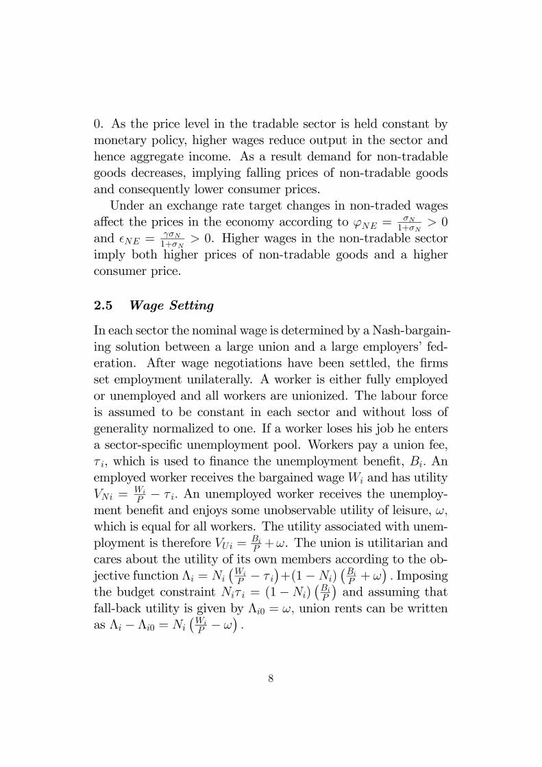
0. As the price level in the tradable sector is held constant bymonetary policy, higher wages reduce output in the sector andhence aggregate income. As a result demand for non-tradablegoods decreases, implying falling prices of non-tradable goodsand consequently lower consumer prices.Under an exchange rate target changes in non-traded wages
affect the prices in the economy according to ϕNE =σN1+σN
> 0and NE =
γσN1+σN
> 0. Higher wages in the non-tradable sectorimply both higher prices of non-tradable goods and a higherconsumer price.
2.5 Wage Setting
In each sector the nominal wage is determined by a Nash-bargain-ing solution between a large union and a large employers’ fed-eration. After wage negotiations have been settled, the firmsset employment unilaterally. A worker is either fully employedor unemployed and all workers are unionized. The labour forceis assumed to be constant in each sector and without loss ofgenerality normalized to one. If a worker loses his job he entersa sector-specific unemployment pool. Workers pay a union fee,τ i, which is used to finance the unemployment benefit, Bi. Anemployed worker receives the bargained wageWi and has utilityVNi =
Wi
P − τ i. An unemployed worker receives the unemploy-ment benefit and enjoys some unobservable utility of leisure, ω,which is equal for all workers. The utility associated with unem-ployment is therefore VUi = Bi
P +ω. The union is utilitarian andcares about the utility of its own members according to the ob-jective function Λi = Ni
¡Wi
P − τ i¢+(1−Ni)
¡Bi
P + ω¢. Imposing
the budget constraint Niτ i = (1−Ni)¡Bi
P
¢and assuming that
fall-back utility is given by Λi0 = ω, union rents can be writtenas Λi − Λi0 = Ni
¡Wi
P − ω¢.
8
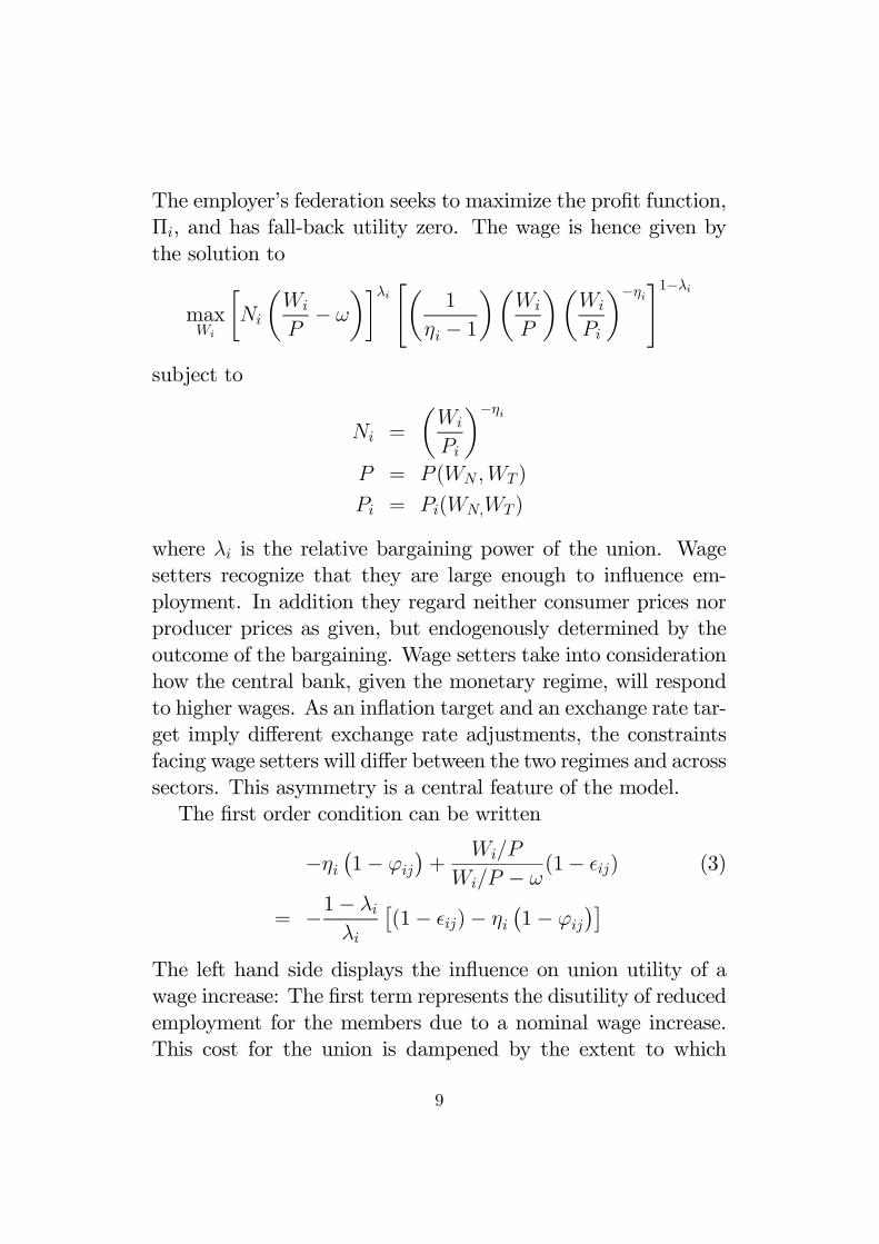
The employer’s federation seeks to maximize the profit function,Πi, and has fall-back utility zero. The wage is hence given bythe solution to
maxWi
·Ni
µWi
P− ω
¶¸λi "µ 1
ηi − 1¶µ
Wi
P
¶µWi
Pi
¶−ηi#1−λisubject to
Ni =
µWi
Pi
¶−ηiP = P (WN ,WT )
Pi = Pi(WN,WT )
where λi is the relative bargaining power of the union. Wagesetters recognize that they are large enough to influence em-ployment. In addition they regard neither consumer prices norproducer prices as given, but endogenously determined by theoutcome of the bargaining. Wage setters take into considerationhow the central bank, given the monetary regime, will respondto higher wages. As an inflation target and an exchange rate tar-get imply different exchange rate adjustments, the constraintsfacing wage setters will differ between the two regimes and acrosssectors. This asymmetry is a central feature of the model.The first order condition can be written
−ηi¡1− ϕij
¢+
Wi/P
Wi/P − ω(1− ij) (3)
= −1− λiλi
£(1− ij)− ηi
¡1− ϕij
¢¤The left hand side displays the influence on union utility of awage increase: The first term represents the disutility of reducedemployment for the members due to a nominal wage increase.This cost for the union is dampened by the extent to which
9
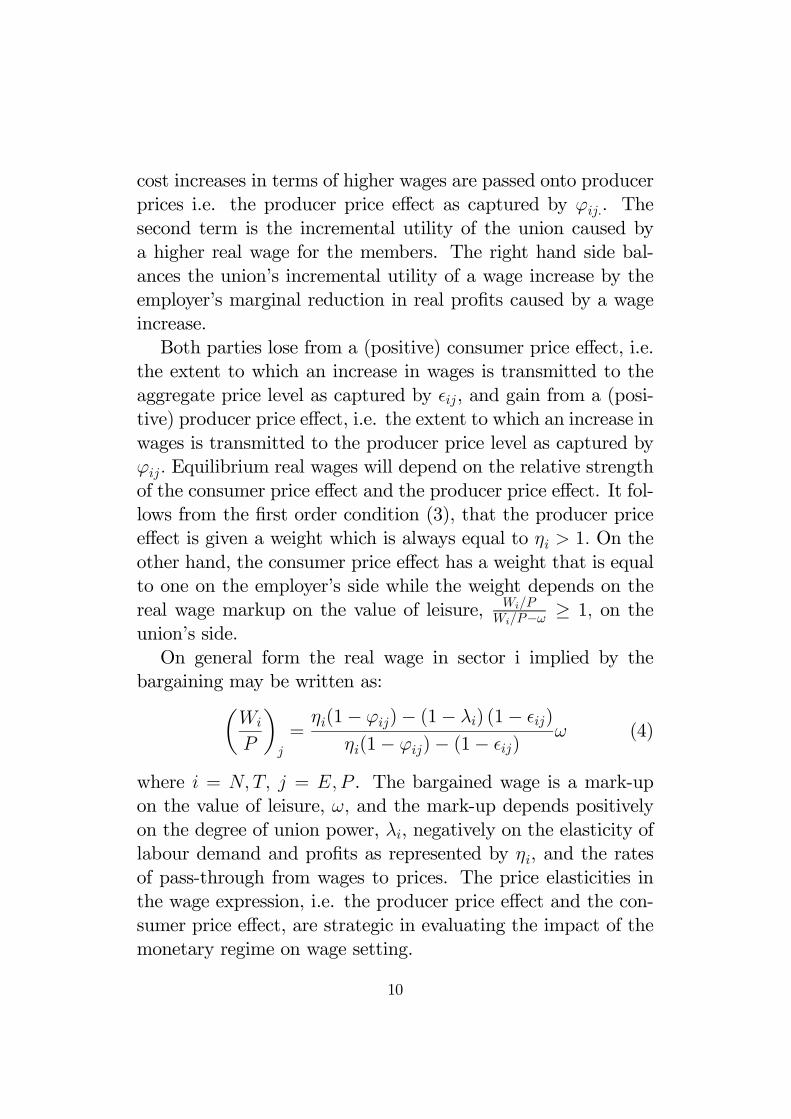
cost increases in terms of higher wages are passed onto producerprices i.e. the producer price effect as captured by ϕij.. Thesecond term is the incremental utility of the union caused bya higher real wage for the members. The right hand side bal-ances the union’s incremental utility of a wage increase by theemployer’s marginal reduction in real profits caused by a wageincrease.Both parties lose from a (positive) consumer price effect, i.e.
the extent to which an increase in wages is transmitted to theaggregate price level as captured by ij, and gain from a (posi-tive) producer price effect, i.e. the extent to which an increase inwages is transmitted to the producer price level as captured byϕij. Equilibrium real wages will depend on the relative strengthof the consumer price effect and the producer price effect. It fol-lows from the first order condition (3), that the producer priceeffect is given a weight which is always equal to ηi > 1. On theother hand, the consumer price effect has a weight that is equalto one on the employer’s side while the weight depends on thereal wage markup on the value of leisure, Wi/P
Wi/P−ω ≥ 1, on theunion’s side.On general form the real wage in sector i implied by the
bargaining may be written as:µWi
P
¶j
=ηi(1− ϕij)− (1− λi) (1− ij)
ηi(1− ϕij)− (1− ij)ω (4)
where i = N, T, j = E,P . The bargained wage is a mark-upon the value of leisure, ω, and the mark-up depends positivelyon the degree of union power, λi, negatively on the elasticity oflabour demand and profits as represented by ηi, and the ratesof pass-through from wages to prices. The price elasticities inthe wage expression, i.e. the producer price effect and the con-sumer price effect, are strategic in evaluating the impact of themonetary regime on wage setting.
10
By inserting the regime-specific elasticities of prices with respectto wages described above in equation (4), it is straightforwardto show that the ranking of regime-specific real wages satisfiesµ
WT
P
¶P
>
µWT
P
¶E
(5)µWN
P
¶E
>
µWN
P
¶P
(6)
This result is consistent with Vartiainen (2002). In order tounderstand the ranking given by (5) and (6), we need to recallhow the producer price effects and the consumer price effectsaffect wages under the two regimes. The impact of these effectson wage formation is summarized in Table 2.The reason why real wages in the traded sector are higher
under inflation targeting than under exchange rate targeting, isthat the (positive) producer price effect under inflation targetingis stronger than the (negative) consumer price effect under ex-change rate targeting. The reversed ranking in the non-tradedsector, is due to the (positive) producer price effect being somuch stronger under exchange rate targeting than under in-flation targeting, that the mitigating (positive) consumer priceeffect under exchange rate targeting is insufficient.
3 Equilibrium Employment
Having established that the monetary regime indeed affects thereal wage in the two sectors, the impact of the monetary regimeon equilibrium (un) employment remains to be analysed. Wenow extend the model by Holden (2003), by providing an ex-plicit expression for equilibrium employment and analyse it.
11
Table 2: Wage formation under different monetary regimesRegime-specific Impact on Wages
elasticitiesTraded Sector
Inflation targetϕTP > 0 +TP = 0 None
Exchange rate targetϕTE = 0 NoneTE < 0 +
Real wage ranking¡WT
P
¢P>¡WT
P
¢E
Non-traded sector
Inflation target
ϕNP > 0 +NP = 0 None
Exchange rate targetϕNE > 0 +NE > 0 -
Real wage ranking¡WN
P
¢E>¡WN
P
¢P
For each regime we have a system consisting of a horizontalwage curve for each sector, equation (4), a labour demand curvein each sector, equation (1) and a relative price determined byequilibrium on the goods market, equation (2). These five equa-tions determine five endogenous variables: WT
P , WN
P , NN , NT andPNPT. Here we focus on the case where production technology is
equal across sectors, i.e. when ηN = ηT = η. Solving the systemabove and using the fact that aggregate employment is given by
12
the sum of employment in the two sectors , i.e. N = NN +NT ,equilibrium employment is given by6
Nj =
µ1
1− γ
¶(1−γ)µ1γ
¶γ µWT
P
¶−(1−γ)(η−1)j
µWN
P
¶−γ(η−1)j
·Ãγ
µWN
P
¶−1j
+ (1− γ)
µWT
P
¶−1j
!(7)
where as before j = E,P and sector-specific wages are given byevaluating equation (4) for both regimes and sectors. Note thatsince the wage curve is horizontal, it is the labour demand curvethat identifies employment in employment-real wage-space. Dueto the complicated functional form, we are not able to derive anexplicit ranking of equilibrium employment. But by simulatingequilibrium employment we focus on some interesting cases thatprovide some insight into the predictions of the model.
3.1 Simulating Equilibrium Employment
The model has several features that are not crucial to the analy-sis of the monetary regime, such as the elasticity of labour de-mand and bargaining power. We can therefore assume λN =λT = λ without altering the central mechanisms of the model.But since the ranking of sector-specific wages, as given by (5)−(6), indicate that the effects of the regime is quite the oppositefor the two sectors, one may suspect that the overall outcome isclosely related to which sector is the dominant one, i.e. whichsector is larger. In what follows we therefore focus on sector sizecaptured by γ and start by looking at some limiting values. Forthe extremely open economy, γ −→ 0, or the closed economy,γ → 1, aggregate employment is unaffected by the monetary
6 Recall that the labor force is normalized to one in each sector, so thataggregate equilibrium unemployment is given by 2−N .
13
Table 3: Simulated threshold values of γ∗, non-traded sector size
Parameter λ ω η γ
.5 1 1.10 .6178
.5 1 1.5 .6823
.5 1 8 .9137
.9 1 1.10 .6616
.9 1 1.5 .7245
.9 1 8 .9296Notes: γ∗ is defined by NP (γ
∗) = NE(γ∗) and NP (γ) > NE(γ) ∀γ < γ∗.
All simulations were carried out using MATLAB 6.5.
regime7. Perhaps this seems surprising at first, but the intuitionis simple: When γ → 0 an exchange rate target is equivalent toan inflation target since the traded sector then constitutes theentire economy and we get P = PT . In the case when γ → 1there is only one feasible regime since the non-traded sector con-stitutes the entire economy; P = PN . In both cases, the modelcollapses.8
However, turning to the intermediate case where 0 < γ < 1it is possible to run some numerical simulations. Some resultsare presented in Table 3 and indicate that for plausible valuesof the labour demand elasticity, relative sector size is crucial forwhich regime generates higher equilibrium employment.The importance of the non-traded sector size, or the openness
of the economy, for the equilibrium outcome is clearly displayedin Figures 1 and 2, demonstrating how aggregate employmentvaries non-linearly with γ.
7 That is, limγ→0Np = limγ→0NE and limγ→1Np = limγ→1NE.8 The result is related to proposition 5 in Cukierman & Lippi (1999),
saying that at least two unions are required in order for the monetary regimeto have an impact on equilibrium employment.
14
Figure 1: Simulated aggregate employment as a function of open-ness ( γ)
Notes: Openness (γ) is measured in percent on the X-axis.NP = employment under an inflation target.NE = employment under an exchange rate target.Parameter values: η = 3/2, λ = .5.
The main simulation result is that equilibrium employment isgenerally higher under an inflation target than under an ex-change rate target in an economy with a non-traded sector thatconstitutes less than 60-70 percent of the economy.9 The resultis explained by one or several of three candidate equations: thereal wage ranking given by equations (5) and (6), and the em-ployment equation (7). There are mainly two channels throughwhich the sector size affects these equations.First, the strength of the real wage ranking in (5) and (6) vary
with γ, since γ enters into the expressions for the consumer andproducer price effects given in Table 1.
9 The results are stronger the more elastic is labor demand (η → ∞).Recalling that η = (1−δ)−1, constant returns to scale, δ → 1 implies η →∞why aggregate employment is higher under inflation targeting than exchangerate targeting under rather general assumptions.
15
Figure 2: Simulated aggregate employment as a function of open-ness ( γ)
Notes: Openness (γ) is measured in percent on the X-axis.NP = employment under an inflation target.NE = employment under an exchange rate target.Parameter values: η = 3/2, λ = .9.
Second, γ enters directly as a parameter in the complicated func-tional form of the employment equation. Since γ enters in sev-eral of these expressions it is not possible to identify one singlereason why employment seems to be higher under inflation tar-geting than exchange rate targeting for rather low values of γ.We can make an attempt by assessing the relative strength ofthe real wage ranking in (5) and (6) while varying γ between 0and 1. The results of this exercise are shown in figures 3 and 4.The ranking in equations (5) and (6) is valid for all plausible
parameter values, more specifically for all γ ∈ (0, 1). However,the strength of the ranking, i.e. the regime differentials
¡WT
P
¢P−¡
WT
P
¢Eand
¡WN
P
¢E−¡WN
P
¢Pare functions of γ since real wages are
functions of the consumer and producer price effects, which inturn are functions of γ. The graphs of the real wage differentials
16
Figure 3: Simulated real wage regime differentials as a functionof openness (γ)
Notes: Openness (γ) is measured in percent on the X-axis.WTP −WTE = traded sector differential.WNE −WNP = non-traded sector differential.Parameter values: η = 3/2, λ = .5.
show that they are larger for extreme values of γ.10 These resultsare explained by taking the limits of the producer and consumerprice effects in Table 1 as γ → 0 and γ → 1, respectively and byevaluating their effects on wage formation summarized in Table2.Perhaps more interestingly, we note that for the calculated
threshold values γ∗, given by the intersection of the graphs inFigures 3 and 4, the real wage differentials are very small. Ittherefore seems likely that the main simulation results are drivenby the functional form of the employment equation rather thanthe regime-specific wage differentials.10 Formally, we note that limγ→0
¡WT
P
¢P− ¡WT
P
¢E= 0, limγ→1
¡WT
P
¢P−¡
WT
P
¢E= ∞ while the reverse is true for non-traded real wage differentials,
i.e. limγ→0¡WN
P
¢E− ¡WN
P
¢P=∞ and limγ→1
¡WN
P
¢E− ¡WN
P
¢P= 0.
17
Figure 4: Simulated real wage regime differentials as a functionof openness (γ)
Notes: Openness (γ) is measured in percent on the X-axis.WTP −WTE = traded sector differential.WNE −WNP = non-traded sector differential.Parameter values: η = 3/2, λ = .9.
To sum up, the simulation results indicate that under rathergeneral assumptions inflation targeting produces higher employ-ment than exchange rate targeting. However, we need actualdata to be able to say something about the real world and inthe following sections we perform an empirical analysis.
4 Empirical Analysis
To empirically assess the importance of the monetary regimefor wages and (un)employment, we use panel data on 17 OECDcountries from the period 1972-2000.11 We focus on countriesthat have combined inflation targets (denoted IT) with floatingexchange rates. The countries included in the study are Aus-11 Data description and definitions are given in the appendix.
18
Table 4: Countries included in the studyCountry Average Regime a Date for Actual Regime
N-sector size Announcement Switch c
of IT b
Australia .24 IT 1993 1994Belgium .29Canada .28 IT 1991 1994Denmark .33Finland .30 (IT) 1993 1994France .28Germany .26Ireland .23Italy .25Japan .21Netherlands .33New Zeeland .23 IT 1990 1993Norway .29Spain .20 (IT) 1995 1996Sweden .33 IT 1993 1995UK .26 IT 1992 1993US .21Notes: Countries excluded due to lack of data: Austria, Greece, Hungary,Iceland, Korea, Luxembourg, Portugal, Switzerland, Turkey.a IT = Inflation Targeting.b Source: Cottarelli & Giannini (1997).c Source: Ball & Sheridan (2003), Table 1. Actual regime switch refers to thedate constant inflation targeting was introduced in the country at hand.
tralia, Canada, New Zeeland, Sweden and the United Kingdom,thus excluding Finland and Spain having combined inflation tar-gets with membership in the EMU. Table 4 lists the countriesin the study together with the years they switched regimes. Weuse two different approaches in testing for the impact of infla-tion targeting on labour markets. First, a very simple difference-in-differences approach, and second, a full-scale dynamic panelframework. Results are presented in Section 5.
19
4.1 A First Simple Test of the Impact of Inflation Tar-geting
When trying to evaluate the impact of a regime switch on avariable, it is important to exercise some caution. It may be thecase that countries that adopt inflation targeting have differentcharacteristics than countries not adopting inflation targets andvice versa. It may therefore be hard to determine whether it isin fact inflation targeting that has changed the situation for tar-geting economies, or if there are some other factors that causesuch a development. For instance, it is hardly surprising thatan economy with hyperinflation has a flatter growth path of in-flation once an inflation target is introduced, while the oppositemay be true for low inflation economies.We avoid this problem by applying the difference-in-differences
technique used by Ball and Sheridan (2003). The idea is to con-trol for regression to the mean by adding initial values to crosssection regressions of mean values of our key variables, calcu-lated before and after the introduction of inflation targeting.Suppose we are interested in evaluating the effect of inflation
targeting on a variable Y . Denote by Ti the point in time incountry i when the country introduced inflation targeting. Fornon-targeters, we choose these breakpoints to be the same forall countries in the group and given by the average year amongtargeters. We then define
ITi =n1 if country i is an inflation targeter
0 otherwise
Suppose data ranges over the period [T0, T ]. We then calculatethe following measures for all countries
20
Y prei =
1
(Ti − T0)
TiXt=T0
Yi,t
Y posti =
1
(T − (Ti + 1))TX
t=Ti+1
Yi,t
for i = 1, ...I. We then run the following regressions
Y posti − Y pre
i = τ + κITi + ζY prei + i (8)
for i = 1, ...I. Including Y prei ensures that we avoid regression
to the mean, i.e. κ, if significant, captures a true effect of tar-geting.12
Although the above method is appealing in its simplicity,it has several drawbacks. First, the collapse of the panel to across-section implies that we are forced to estimate over very fewobservations. Second, we would like to allow for a richer specifi-cation in testing the predictions of the model, and this calls fora more sophisticated method. Consequently, we proceed by anattempt to turn the theoretical model into an econometric spec-ification, accounting for possible effects of inflation targeting.
4.2 Taking the Model to the Data
An important feature of the theoretical model is the fact thatthe two sectors are affected differently by the monetary regime.In testing the implications of the model one should optimally usesectorial data on all variables suggested by the model. However,due to data unavailability, we can only partly meet this require-ment by using sectorial data on wages, but aggregate data onthe other variables. The empirical analysis thus hinges on the12 A sketchy proof is given by Ball and Sheridan (2003).
21
assumption that for instance bargaining power is equal acrosssectors.Recall the main prediction by the theoretical model as given
by equations (5) and (6): The traded sector real wage is higherunder an inflation target than under an exchange rate targetwhile the non-traded sector real wage is lower under an inflationtarget than under an exchange rate target. In an attempt totest the empirical validity of this result, we start by estimatingreal wage equations for the traded and non-traded sectors.The bargained real wage in sector i as given by equation (4) is
a function of bargaining power (λi) and the regime-specific priceelasticities, i.e the consumer price effect ( ij) and the producerprice effect (ϕij). Empirically, we summarize these mechanismsby estimating the following function
WiP = f(UNION,∆ logCPI,∆ logPPI, u, RHO) (9)
where WiP is the empirical counterpart to the theoretical realwage in sector i, UNION is the empirical counterpart to bar-gaining power, and ∆ logCPI and ∆ logPPI are the consumerand the producer price effects respectively. Two additional vari-ables, frequently used in the literature, are added ad hoc to theeconometric model: The unemployment rate (u), presumablyaffecting the bargaining power of the worker and the unemploy-ment benefit (RHO), presumably affecting the value of beingunemployed.13
Note that although we have theoretical predictions for howbargaining power and the consumer and producer price effectsaffect the real wage in general, according to equation (4), theelasticities of the real wages with respect to these variables are13 In our theoretical model we assume that unions bear the costs of their
own unemployment, by letting the workers finance the members that arerendered unemployed. Therefore, the unemployment benefit does not showup in the wage equation.
22
not regime-specific. Specifically, we expect f1 > 0, f2 < 0, f3 > 0and that these effects are equally strong regardless of regime.What we do have is theoretical predictions for equilibrium val-ues of the consumer and producer price effects under differentmonetary regimes. However, we do not have any theoreticalpredictions for how an arbitrary incremental change in the con-sumer and producer price effects affects the real wage underdifferent monetary regimes. Consequently, we include these ar-guments in (9) merely as controls, and focus on possible effectsof the monetary regime captured by dummy variables. For thead hoc variables, the conventional priors in the literature aref4 < 0 and f5 > 0, respectively.We also estimate unemployment equations based on (7), as-
suming that the labour force is constant. Our simulation resultssuggest that unemployment should be lower under inflation tar-geting provided that the non-traded sector constitutes less than60-70 percent of the economy. Actual data, presented in Ta-ble 2, suggests that the size of the non-traded sectors of thecountries in the study is approximately 27 percent on average.We therefore expect unemployment levels to fall when inflationtargeting is introduced. Since real wages are endogenously de-termined in the model, we estimate reduced form equivalents tothe unemployment equation suggested by (7). The unemploy-ment equation can be described by the following function
u = g(γ, UNION,∆ logCPI,∆ logPPI,RHO) (10)
where we again include the unemployment benefit as an ad hocdeterminant. Following the discussion above, we have no priorsfor the signs of these effects. We focus on the effect of infla-tion targeting as captured by dummy variables and pay littleattention to the explanatory variables suggested by the abovefunction.
23
4.3 Econometric Method
Having established which variables should be included in theempirical study, we need to determine how to isolate the effectof the monetary regime on wages and unemployment. Supposewe are interested in estimating the model
Yit =Xj
αjXijt + it (11)
where we have longitudinal data on j = 1, ..., J independentvariables, i = 1, ..., I countries over the period t = 1, ..., T . Weare interested in assessing the impact of inflation targeting onthe estimated relationship, and define
ITit =n1 if country i has an inflation target at time t
0 otherwise
We then estimate the following model
Yit =Xj
αjXijt + ITit ∗Xj
βjXijt + µITit + it (12)
where i = 1, ..., I, i.e. we interact the inflation target with theexplanatory variables and estimate the model on all countriesin the sample. Suppose for simplicity that all variables are inlogs. The interpretation of βj is that countries that at somepoint have introduced an inflation target have an elasticity of Ywith respect to X that is on average βj per cent higher than acountry without an inflation target. Moreover they have a valueof Y that is on average µ per cent higher than non-inflationtargeting countries.In order to verify that it is the introduction of the infla-
tion target rather than the properties of the specific economiesthat causes a potential difference between inflation targeting
24
economies and economies without inflation targets, we next fo-cus on countries that have implemented inflation targets. De-note the number of countries that have adopted and imple-mented inflation targets by IIT . We then run the followingregression
Yit =Xj
θjXijt + ITit ∗Xj
ξjXijt + νITit + it (13)
for i = 1, ..., IIT , i.e. for inflation targeting countries only. As inthe previous model, interacting all variables with the IT-dummyallows for the impact of the independent variables on the de-pendent variable being regime-specific. Although we have notheoretical predictions for how the regime should alter the elas-ticities in the models, we prefer to start from a rich specificationin order to avoid imposing possibly false constraints on the data.The estimated coefficient of the IT -dummy, υ, now captures
a possible structural break at the time the target was imple-mented. Provided that E( it) = 0, we obtain
E(Yit|ITit = 0) =Xj
θjXijt
E(Yit|ITit = 1) = ν +Xj
(θj + ξj)Xijt
To test the hypothesis that there is a structural break at thetime the inflation target was introduced, we look for significantestimates of ν and the ξj : s. A significant estimate of ν indi-cates that the introduction of an inflation target has shifted thelevel of Y by µ percent on average, an effect that is indeed dueto the introduction of inflation targeting. Hence, by this two-step procedure, we avoid the problem of regression to the mean(compare the discussion above).Finally note that the model provides theoretical predictions
about levels in wages and unemployment, but offers no insight
25
into growth rates. We can therefore not take into account non-stationarities that are likely to be present in some of the data byestimating first differences when testing the theoretical model.Lags of variables are used when we think they affect future wageformation and unemployment. In order to reduce possible auto-correlation we add a lag of the dependent variables to the inde-pendent variables. We estimate fixed effects models, controllingfor the overall evolution of the world economy by adding yeardummies.
5 Empirical Results
5.1 The Difference-in-differences Approach
The results from estimating equation (8) based on the difference-in-differences approach described above are given in Table 5.Throughout we perform some sensitivity analysis by using along period (starting 1972) and a short period (starting 1985)when calculating the average values prior to the inflation target,i.e. the values referred to as initial values in the tables.In order to test the method, we first investigate whether in-
flation rates have decreased in countries that have introducedinflation targets. Contrary to Ball and Sheridan (2003), the re-sults in columns (1) and (2) indicate that inflation rates decreasewhen inflation targets are introduced and implemented.Turning to the implications of the theoretical model, we next
investigate whether the sectorial real wage ranking according toequations (5) and (6) is confirmed by the data. The results incolumns (3)-(6) imply that the inflation target has no significanteffects on real wages. In addition, the estimations in columns (7)and (8) indicate that unemployment rates are unaffected by theinflation target. Hence, this simple test indicates that importantlabour market variables are unaffected by inflation targeting.
Notes: Dependent variable defined as ∆Y = Y post − Y pre.IT refers to the year the inflation target was implemented.Inflation π is defined as π = d logCPI.White Heteroscedasticity-Consistent standard errors in parenthesis.Significance codes: ***=1%, **=5%, *=10%.
Following Ball and Sheridan, we distinguish between the datethe target was announced and the date it was implemented(compare Table 4), and re-run all regressions using announce-ment dates instead of implementation dates (as in Table 5). Asshown in Table A1 in the Appendix, the main result is robust tothis modification, i.e. wages and unemployment are unaffectedby the inflation target.
5.2 The Wage Equations
We next turn to the results from estimating the real wage equa-tions implied by the theoretical model.Table 6 reports the estimates of the traded sector real wage
equation, equation (9), along with interaction terms for inflation
27
Table 6 : Estimations of traded-sector real wage equations1972-2000. Dependent Variable: logRWT , fixed effects
Notes: White Heteroscedasticity-Consistent standard errors in parenthesis.Significance codes: ***=1%, **=5%, *=10%.
targeting (IT ) under the assumption of fixed country-specific ef-fects. The estimates in column (1) show a strong autoregressivecoefficient, indicating high real wage persistence. The estimateof the consumer-price-effect (d logCPI−1), the producer-price
28
effect (d logPPI−1) and the unemployment rate (u−1) all displayexpected signs and are statistically significant at conventionallevels whereas this is not true for union density (UNION−1) andunemployment benefits (RHO−1). In column (2) we isolate theeffect of the inflation target, removing the insignificant interac-tion terms. The results show that inflation targeters on averagehave higher real wages in the traded sector than non-targeters.In order to determine whether this is a true effect of targeting,we estimate over IT-countries only, which yields the estimates incolumns (3) and (4). When reducing the model and focusing onthe IT-dummy in isolation in column (4), we see that inflationtargeting indeed causes higher real wages in the traded sector.This is consistent with our theoretical model, and evidence thatinflation targeting matters for wage formation. However, includ-ing year dummies in columns (5)-(8) indicates that traded sectorreal wages are higher in IT-countries, but that this effect is notdue to inflation targeting.Table 7 reports results from estimating non-traded sector real
wage equations. Unlike in Table 6, the strategic explanatoryvariables such as the consumer and producer effects have theexpected signs, but on low levels of significance. Contrary tothe results for the traded sector in Table 6, the estimate ofthe IT-dummy in column (2) shows that the real wage tendsto be lower in the non-traded sector in IT-countries. However,the insignificant estimate of the coefficient for the IT-dummy incolumn (4), suggests that non-traded real wage levels are unaf-fected by the introduction of inflation targeting. Hence, the factthat non-traded real wages are lower in IT-countries, is due toother factors than the introduction of inflation targeting. Themain results do not change when year dummies are included incolumns (5)-(8).
29
Table 7 : Estimations of non traded-sector real wage equations1972-2000. Dependent Variable: logRWN , fixed effects
Notes: White Heteroscedasticity-Consistent standard errors in parenthesis.Significance codes: ***=1%, **=5%, *=10%.
A natural step is then to investigate whether or not the monetaryregime matters for unemployment. Recall that the simulationresults show that unemployment levels are likely to be lower un-der inflation targeting than under exchange rate targeting.
30
Table 8 : Estimations of reduced-form unemployment growthequations 1972-2000. Dependent Variable: du, fixed effects
(1) (2) (3) (4) (5) (6) (7) (8)
All All IT IT All All IT ITdu−1 .373*** .362*** .394*** .336*** .337*** .327*** .270* .262**
Notes: White Heteroscedasticity-Consistent standard errors in parenthesis.Significance codes: ***=1%, **=5%, *=10%.
However, due to severe non-stationarities in the unemploymentseries, estimating unemployment equations in levels might re-flect spurious correlations rather than genuine relationships. Wehave therefore chosen to estimate unemployment equations interms of first differences, using the explanatory variables sug-gested by theory. Estimating such equations indicate how theunemployment growth rate is affected by the monetary regime.However, this is an effect for which we have no theoretical predic-tions and the models should not be seen as tests of the theory.14
14 In fact we made an attempt at estimating unemployment equations in
31
According to theory, the regime may cause shifts in unemploy-ment levels, and such shifts are not captured in these equa-tions. The results from estimating reduced-form unemploymentgrowth equations are given in Table 8. The models in columns(1) and (2) show that IT-countries have lower unemploymentgrowth rates than other countries, and the estimates in columns(3) and (4) suggest that these features are indeed due to infla-tion targeting. However, these effects vanish when controllingfor aggregate effects by including year dummies in columns (5)-(8).In sum, there is weak empirical evidence for some of the the-
oretical predictions of the model. Traded-sector real wages arehigher under inflation targeting. We identify this effect as beingdue to targeting and not to common characteristics of target-ing economies. These effects vanish when year dummies areincluded. There is no support for the corresponding rankingof non-traded sector real wages. The unemployment equationshould not be seen as a test of the theory, but lends some sup-port to unemployment growth rates being lower under inflationtargeting.One should be aware that the dynamic panel approach gen-
erating the results in Tables 6 and 7 is not without problems.First, we note the suspiciously high goodness of fit. The R2-adjusted of .99 leads us to suspect that there may be trendspresent in the data, and that these trends may account for theresults. Therefore, at first glance it seems like a good idea touse de-trended data. Unfortunately, de-trending the data im-plies removing structural shifts that may be due to the inflationtarget.15 Since the aim of the analysis is to test for possible ef-
levels, but the results were uninterpretable and plagued by heavy autocorre-lation.15 Suppose there is a positive shift in levels caused by the inflation target.
Removing a trend in such a graph means removing a steeper trend than the
32
fects of inflation targeting, de-trending is an inappropriate pro-cedure.Second, the OLS-estimates might be biased and inconsistent
when including an autoregressive component. On one hand,dropping the lagged dependent variable generates severe auto-correlation. The suggested remedy is to use GMMwhen estimat-ing dynamic panels, but since we have very few cross-sectionalobservations, in particular when estimating over inflation tar-geting countries only, GMM estimation is not an option. Onthe other hand, the bias in the OLS-estimates tends to zero asT tends to infinity, why the bias in our sample of 29 years, islikely to be small.Third, the high estimate of the autoregressive component im-
plies that it would be favorable to estimate first differences ofthe dependent variable. But since we only have theoretical pre-dictions for levels of the variables, first difference estimation isnot an option when testing the theory.Fourth, an obvious limitation is that we only to some extent
can use sectorial data when estimating the model. Until bettersectorial data is available, we conclude that the results should beinterpreted with caution. In sum, the results presented in thispaper suggests that inflation targeting might matter for labourmarkets.
6 Concluding Remarks
This paper analyses whether or not inflation targeting mattersfor the labour market outcome. The analysis is based on simu-lation results and panel data regressions on 17 OECD-countriesof which five countries have combined an explicit inflation tar-get with floating exchange rates during the 1990s. The main
actual trend, i.e. the trend subject to a positive parallell shift at the timethe inflation target is introduced.
33
conclusion of the paper is that inflation targeting might matterfor labour markets.The simulation results suggest that under rather general as-
sumptions inflation targeting produces lower unemployment (orhigher employment) than exchange rate targeting. The size ofthe non-traded sector, i.e. the degree of openness of the econ-omy, is crucial to which regime generates higher equilibriumun(employment).Consistent with the theoretical model, there is some empiri-
cal evidence that traded sector real wages are higher under infla-tion targeting while non-traded sector real wages are unaffectedby inflation targeting. Finally we find some evidence that theunemployment growth path is flatter in countries that have in-troduced inflation targeting, an effect that is indeed due to themonetary regime.
34
References
[1] Ball, L. & Sheridan, N. (2003), ”Does Inflation TargetingMatter”, NBER Working Paper, No. 9577
[2] Bratsiotis, G. & Martin, C. (1999), ”Stabilization, Pol-icy Targets and Unemployment in Imperfectly CompetitiveEconomies”, Scandinavian Journal of Economics, Vol. 101No. 2
[3] Calmfors, L. (2001), ”Wages and Wage-Bargaining Institu-tions in the EMU - A Survey of the Issues”, Empirica
[4] Clifton, E.V., Hyginus, L. & Wong, C-H. (2001), ”InflationTargeting and the Unemployment-Inflation trade-off”, IMFWorking Paper 01/166, International Monetary Fund
[5] Cottarelli, C. & Giannini, C. (1997), ”Credibility WithoutRules? Monetary Frameworks in the Post-Bretton WoodsEra”, IMF Occasional Paper 154, IMF
[6] Cukierman, A. & Lippi, F. (1999), ”Central bank Inde-pendence, Centralization of Wage Bargaining, Inflation andUnemployment: Theory and Some Evidence”, EuropeanEconomic Review, Vol. 43
[7] Holden, S., (2003), “Wage setting under Different MonetaryRegimes”, Economica, Vol. 70
[8] Neuman, M.J.M & von Hagen, J. (2002), ”Does InflationTargeting Matter? Commentary”, Federal reserve Bank ofSt. Louis Review, Vol. 84 no. 4 (July-Aug 2002)
[9] Sheridan, N. (2001), ”Inflation Dynamics”, Johns HopkinsUniversity, PhD Dissertation
35
[10] Vartiainen, J., (2002), “Relative Wages in Monetary Unionand Floating”, Scandinavian Journal of Economics, Vol.104, No. 2
36
Appendix
Data are from the OECD. Data on unemployment benefits and
trade union density are from the OECD database Labour Mar-
ket Statistics. All other data are from OECD Economic Outlook,
No. 70.
ut : Unemployment rate.CPIt : Consumer price indexPPIt : The GDP-deflatorγt : Non-traded sector size. Government consumption
as a share of total consumptionUNIONt : Trade union density ratesRHOt : Index of gross unemployment benefit ratesRWTt : Real traded-sector consumer wage, hourly wage rate
deflated by consumer pricesRWNt : Real non-traded-sector consumer wage, hourly wage
Notes: Dependent variable defined as ∆Y = Y post − Y pre.
IT refers to the year the inflation target was implemented.
Inflation π is defined as π = d logCPI.
White Heteroscedasticity-Consistent standard errors in parenthesis.
Significance codes: ***=1%, **=5%, *=10%.
38
Working Paper Series/Arbetsrapport FIEF Working Paper Series was initiated in 1985. A complete list is available from FIEF upon request. Information about the series is also available at our website: http://www.fief.se/Publications/WP.html. 2001 166. Hansson, Pär, “Skill Upgrading and Production Transfer within Swedish Multinationals in the 1990s”, 27 pp. 167. Arai, Mahmood and Skogman Thoursie, Peter, “Incentives and Selection in Cyclical Absenteeism”, 15 pp. 168. Hansen, Sten and Persson, Joakim, “Direkta undanträngningseffekter av arbetsmarknadspolitiska åtgärder”, 27 pp. 169. Arai, Mahmood and Vilhelmsson, Roger, ”Immigrants’ and Natives’ Unemployment-risk: Productivity Differentials or Discrimination?”, 27 pp. 170. Johansson, Sten och Selén, Jan, ”Arbetslöshetsförsäkringen och arbetslösheten (2). Reformeffekt vid 1993 års sänkning av ersättningsgraden i arbetslöshetsförsäkringen?”, 39 pp. 171. Johansson, Sten, ”Conceptualizing and Measuring Quality of Life for National Policy”, 18 pp. 172. Arai, Mahmood and Heyman, Fredrik, “Wages, Profits and Individual Unemployment Risk: Evidence from Matched Worker-Firm Data”, 27 pp. 173. Lundborg, Per and Sacklén, Hans, “Is There a Long Run Unemployment- Inflation Trade-off in Sweden?”, 29 pp. 174. Alexius, Annika and Carlsson, Mikael, “Measures of Technology and the Business Cycle: Evidence from Sweden and the U.S.”, 47 pp. 175. Alexius, Annika, “How to Beat the Random Walk”, 21 pp. 2002 176. Gustavsson, Patrik, “The Dynamics of European Industrial Structure”, 41 pp. 177. Selén, Jan, “Taxable Income Responses to Tax Changes – A Panel Analysis of the 1990/91 Swedish Reform”, 30 pp. 178. Eriksson, Clas and Persson, Joakim, “Economic Growth, Inequality, Democratization, and the Environment”, 21 pp.
179. Granqvist, Lena, Selén, Jan and Ståhlberg, Ann-Charlotte, “Mandatory Earnings-Related Insurance Rights, Human Capital and the Gender Earnings Gap in Sweden”, 21 pp. 180. Larsson, Anna, “The Swedish Real Exchange Rate under Different Currency Regimes”, 22 pp. 181. Heyman, Fredrik, “Wage Dispersion and Job Turnover: Evidence from Sweden”, 28 pp. 182. Nekby, Lena, “Gender Differences in Recent Sharing and its Implications for the Gender Wage Gap”, 22 pp. 183. Johansson, Sten and Selén, Jan, “Coping with Heterogeneities in the Difference in Differences Design”, 13 pp. 184. Pekkarinen, Tuomas and Vartiainen, Juhana, “Gender Differences in Job Assignment and Promotion in a Complexity Ladder of Jobs”, 27 pp. 185. Nekby, Lena, “How Long Does it Take to Integrate? Employment Convergence of Immigrants and Natives in Sweden”, 33 pp. 186. Heyman, Fredrik, “Pay Inequality and Firm Performance: Evidence from Matched Employer-Employee Data”, 38 pp. 187. Lundborg, Per and Rechea, Calin, “Will Transition Countries Benefit or Lose from the Brain Drain?”, 18 pp. 2003 188. Lundborg, Per and Sacklén, Hans, “Low-Inflation Targeting and Unemployment Persis-tence”, 34 pp. 189. Hansson, Pär and Lundin,Nan Nan, “Exports as an Indicator on or Promoter of Success-ful Swedish Manufacturing Firms in the 1990s”, 39 pp. 190. Gustavsson, Patrik and Poldahl, Andreas, “Determinants of Firm R&D: Evidence from Swedish Firm Level Data”, 22 pp. 191. Larsson, Anna and Zetterberg, Johnny, “Does Inflation Targeting Matter for Labour Markets? Some Empirical Evidence”, 38 pp.