Dominant Currency Paradigm A New Model for Small Open Economies * Camila Casas Federico J. D´ ıez Banco de la Rep ´ ublica Federal Reserve Bank of Boston Gita Gopinath Pierre-Olivier Gourinchas Harvard University and NBER UC at Berkeley and NBER August 7, 2017 Abstract Most trade is invoiced in very few currencies. Despite this, the Mundell-Fleming bench- mark and its variants focus on pricing in the producer’s currency or in local currency. We model instead a ‘dominant currency paradigm’ for small open economies characterized by three features: pricing in a dominant currency; pricing complementarities, and imported input use in production. Under this paradigm: (a) the terms-of-trade is stable; (b) dominant currency exchange rate pass-through into export and import prices is high regardless of destination or origin of goods; (c) exchange rate pass-through of non-dominant currencies is small; (d) expenditure switching occurs mostly via imports, driven by the dollar exchange rate while exports respond weakly, if at all; (e) strengthening of the dominant currency rel- ative to non-dominant ones can negatively impact global trade; (f) optimal monetary policy targets deviations from the law of one price arising from dominant currency uctuations, in addition to the ination and output gap. Using data from Colombia we document strong support for the dominant currency paradigm. * We thank Richard Baldwin, Charles Engel, Christopher Erceg, Jordi Gal´ ı, Philip Lane, Brent Neiman, for very useful comments. We thank Omar Barbiero, Vu Chau, Tiago Fl´ orido, Jianlin Wang for excellent research assistance and Enrique Montes and his team at the Banco de la Rep´ ublica for their help with the data. e views expressed in this paper are those of the authors and do not indicate concurrence by other members of the research sta or principals of the Board of Governors, the Federal Reserve Bank of Boston, or the Federal Reserve System. e views expressed in the paper do not represent those of the Banco de la Rep´ ublica or its Board of Directors. Gopinath acknowledges that this material is based upon work supported by the NSF under Grant Number #1061954 and #1628874. Any opinions, ndings, and conclusions or recommendations expressed in this material are those of the author(s) and do not necessarily reect the views of the NSF. All remaining errors are our own.
Transcript
Dominant Currency ParadigmA New Model for Small Open Economies∗
Camila Casas Federico J. DıezBanco de la Republica Federal Reserve Bank of Boston
Gita Gopinath Pierre-Olivier GourinchasHarvard University and NBER UC at Berkeley and NBER
August 7, 2017
Abstract
Most trade is invoiced in very few currencies. Despite this, the Mundell-Fleming bench-mark and its variants focus on pricing in the producer’s currency or in local currency. Wemodel instead a ‘dominant currency paradigm’ for small open economies characterized bythree features: pricing in a dominant currency; pricing complementarities, and importedinput use in production. Under this paradigm: (a) the terms-of-trade is stable; (b) dominantcurrency exchange rate pass-through into export and import prices is high regardless ofdestination or origin of goods; (c) exchange rate pass-through of non-dominant currenciesis small; (d) expenditure switching occurs mostly via imports, driven by the dollar exchangerate while exports respond weakly, if at all; (e) strengthening of the dominant currency rel-ative to non-dominant ones can negatively impact global trade; (f) optimal monetary policytargets deviations from the law of one price arising from dominant currency uctuations,in addition to the ination and output gap. Using data from Colombia we document strongsupport for the dominant currency paradigm.
∗We thank Richard Baldwin, Charles Engel, Christopher Erceg, Jordi Galı, Philip Lane, Brent Neiman, for very usefulcomments. We thank Omar Barbiero, Vu Chau, Tiago Florido, Jianlin Wang for excellent research assistance and EnriqueMontes and his team at the Banco de la Republica for their help with the data. e views expressed in this paper arethose of the authors and do not indicate concurrence by other members of the research sta or principals of the Board ofGovernors, the Federal Reserve Bank of Boston, or the Federal Reserve System. e views expressed in the paper do notrepresent those of the Banco de la Republica or its Board of Directors. Gopinath acknowledges that this material is basedupon work supported by the NSF under Grant Number #1061954 and #1628874. Any opinions, ndings, and conclusions orrecommendations expressed in this material are those of the author(s) and do not necessarily reect the views of the NSF.All remaining errors are our own.
1 Introduction
Nominal exchange rates have always been at the center of erce economic and political debates onspillovers, currency wars, and competitiveness. It is easy to understand why: in the presence of pricerigidities, nominal exchange rate uctuations are associated with uctuations in relative prices andtherefore have consequences for real variables such as the trade balance, consumption, and output.
e relationship between nominal exchange rate uctuations and other nominal and real vari-ables depends critically on the currency in which prices are rigid. e rst generation of New Key-nesian (NK) models, the leading paradigm in international macroeconomics, assumes prices aresticky in the currency of the producing country. Under this ‘producer currency pricing’ paradigm(PCP ), the law of one price holds and a nominal depreciation raises the price of imports relative toexports (the terms-of-trade) thus improving competitiveness. is paradigm was developed in theseminal contributions of Mundell (1963) and Fleming (1962), Svensson and van Wijnbergen (1989),and Obstfeld and Rogo (1995).
ere is, however, pervasive evidence that the law of one price fails to hold. Out of this ob-servation grew a second pricing paradigm. In the original works of Bes and Devereux (2000) andDevereux and Engel (2003), prices are instead assumed to be sticky in the currency of the destinationmarket. Under this ‘local currency pricing’ paradigm (LCP ), a nominal depreciation lowers the priceof imports relative to exports, a decline in the terms-of-trade, thus worsening competitiveness. Bothparadigms have been extensively studied in the literature and are surveyed in Corsei et al. (2010).
Recent empirical work using granular data on international prices questions the validity of bothapproaches. Firstly, there is very lile evidence that the best description of pricing in internationalmarkets follows either PCP or LCP . Instead, the vast majority of trade is invoiced in a smallnumber of ‘dominant currencies’, with the U.S. dollar playing an outsized role. is is documentedin Goldberg and Tille (2008) and in Gopinath (2015). Moreover, these prices are found to be rigid forsignicant durations in their currency of invoicing, as documented by Gopinath and Rigobon (2008)and Fitzgerald and Haller (2012). Secondly, exporters price in markets characterized by strategiccomplementarities in pricing that give rise to variations in the elasticity of demand and desiredmark-ups.1 irdly, most exporting rms employ imported inputs in production reducing the valueadded content of exports.2 e workhorse NK models in the literature instead assume constant
1Burstein and Gopinath (2014) survey the evidence on variable mark-ups.2e fact that most exporters are also importers is now well documented in the literature. See Bernard et al. (2009), Kugler
and Verhoogen (2009), Manova and Zhang (2009) among others. is is also reected in the fact that value added exports aresignicantly lower than gross exports, particularly for manufacturing, as documented in the works of Johnson (2014) and
1
demand elasticity and/or abstract from intermediate inputs.Based on these observations, this paper proposes an alternative: the ‘dominant currency paradigm’
(DCP ). Under DCP , rms set export prices in a dominant currency (most oen the dollar) andchange them infrequently. ey face strategic complementarities in pricing, so that desired mark-ups vary over time and across destination markets. Finally, there is roundabout production, withdomestic and foreign inputs employed in production. With these assumptions, the model departsfundamentally from the canonical NK small open economy model a la Galı and Monacelli (2005).
We emphasize the following main results. First, at both short and medium horizons the terms-of-trade is stable, playing lile to no role in expenditure switching. Second, the dominant currencyexchange rate pass-through into export and import prices is high, regardless of the destination ororigin of goods. ird, the exchange rate pass-through of non-dominant currencies is negligible.Fourth, while depreciations have a limited expansionary impact on exports, expenditure switchingstill occurs through imports, arising from uctuations in the relative price of imported to domesticgoods. In turn, these are driven by movements in a country’s exchange rate relative to the dominantcurrency, regardless of the country of origin of the imported goods. Fih, a strengthening of thedominant currency relative to non-dominant ones can negatively impact global trade. Sixth, opti-mal monetary policy targets deviations from the law of one price arising from uctuations in thedominant currency, in addition to the ination and output gap.
Using customs data for a representative small open economy, Colombia, we document strongsupport for the predictions of the model.
Sections 2 and 3 present the baseline model and describe in detail its predictions for the terms-of-trade, exchange rate pass-through, and the impact of monetary policy shocks across pricing regimes.In contrast to the PCP and LCP paradigms, DCP is associated with stable terms-of-trade. isstability, however, diers from predictions of models with exible prices and strategic complementar-ities in pricing such as Atkeson and Burstein (2008). Unlike these models, the terms-of-trade stabilityis associated with volatile movements of the relative price of imported to domestic goods for non-dominant (currency) countries that will be the focus of our analysis. Furthermore, this volatility isdriven by uctuations in the value of the country’s currency relative to the dominant currency, re-gardless of the country of origin of the imported goods. Consequently, when a country’s currencydepreciates relative to the dominant currency, all else equal, it reduces its demand for imports fromall countries.Johnson and Noguera (2012). Amiti et al. (2014) present empirical evidence of the inuence of strategic complementaritiesin pricing and of imported inputs on pricing decisions of Belgian rms.
2
In the case of exports, in contrast to PCP , which associates exchange rate depreciations with in-creases in quantities exported,DCP predicts a negligible impact on goods exported to the dominant-currency destination. For exporting rms whose dominant currency prices are unchanged there isno increase in exports. For those rms changing prices the rise in marginal cost following the risein the price of imported inputs and the complementarities in pricing dampen their incentive to re-duce prices, leaving exports mostly unchanged. e impact on exports to non-dominant currencydestinations depends on the uctuations of the exchange rate of the destination country currencywith the dominant currency. If the exchange rate is stable then DCP predicts a weak impact onexports to non-dollar destinations. On the other hand, if the destination country currency weakens(strengthens) relative to the dominant currency it can lead to a decline (increase) in exports.
Taken together, we nd that the ination-output trade o in response to a monetary policy shock(under an ination targeting monetary rule) worsens under DCP relative to PCP . at is, a mon-etary rate cut raises ination by much more than it increases output, as compared to PCP .
Fluctuations in the value of dominant currencies can also have implications for cyclical uctu-ations in global trade (the sum of exports and imports). Under DCP , a strengthening of dominantcurrencies relative to non-dominant ones is associated with a decline in imports across the periph-ery without a commensurate increase in exports, thus negatively impacting global trade. In contrast,in the case of PCP , the rise in export competitiveness for the periphery generates an increase inexports. Moreover, the increase in exports dampens the decline in imports as production relies onimported intermediate inputs. In the case of LCP , both the import and export response is muted sothe impact on global trade is weak, but remains positive.
Section 4 then proceeds to test the novel empirical predictions of our model for a small open econ-omy, Colombia, that is representative of emerging markets in its heavy reliance on dollar invoicing,with 98.3% (98.4%) of its exports (manufacturing exports) invoiced in dollars.
We document that, as predicted by DCP , the pass-through into import and export (Colombian)peso prices measured as the elasticity relative to the peso-dollar exchange rate starts out high forimport prices and export prices and then gradually declines over time. is is true regardless of theorigin of imports or destination of exports. In the case of export prices to dollar destinations, thecontemporaneous pass-through estimate is 84% while the cumulative pass-through slowly decreasesaer two years to 56%. In the case of import prices from dollar origins, the pass-through is veryhigh, around 100%, and the cumulative eect aer two years declines to 81%. For exports (imports) to(from) non-dollar destinations, the estimated pass-through starts at around 86% (87%) and decreases
3
to 47% (49%) aer two years.Secondly, we nd that, conditional on the peso-dollar exchange rate, the bilateral exchange
rate is quantitatively insignicant as an explanatory factor in bilateral transactions with non-dollareconomies. Unconditionally, the pass-through of the bilateral exchange rate into peso export pricesto non-dollar destinations is 70% at the annual horizon. However, when we control for the peso-dollar exchange rate the coecient on the bilateral exchange rate drops to 9% while the coecienton the peso-dollar exchange rate is 70%. ese predictions are also consistent with DCP .
irdly, we also nd that, following a weaker peso/dollar exchange rate, the pass-through toexport quantities to dollar destinations is mainly insignicantly dierent from zero while there isa pronounced decline in quantities imported from both dollar and non-dollar countries. Exports tonon-dollar destinations also decline. Further, when quantities respond, the relevant exchange rate isthe peso/dollar exchange rates as opposed to the bilateral exchange rate for both export and importquantities.
Lastly, while Colombia’s overall terms-of-trade is very volatile and strongly correlated with theexchange rate, when we strip out commodity prices we nd the terms-of-trade to be highly stable—afeature consistent with the predictions of DCP .
To further compare the dierent pricing paradigms we simulate in Section 5 a model economythat is subject to commodity price shocks, productivity shocks, and third country exchange rateshocks, and test its ability to match the data. As the model nests DCP , PCP and LCP we canevaluate the success of the various paradigms. Using a combination of calibration and estimation wedocument that the data strongly rejects the PCP and LCP paradigms in favor of DCP .
e data also favors a model with strategic complementarities in pricing and imported input use.For example, under our benchmark DCP specication we obtain, in line with the data, the exportpass-through at four quarters to both dollar and non-dollar destinations to be 65%. Instead when weshut down strategic complementarities and imported input use the predicted pass-through declinesby a half to 30%.
Section 6 derives optimal monetary policy for a small open economy with dominant currencypricing under parameter restrictions similar to Galı and Monacelli (2005). e second-order approx-imation to the welfare loss function under dominant currency pricing diers from that under PCP :in addition to ination and the output gap, it includes a term that captures misalignment due to thefailure of the law of one price for Home goods driven by dominant currency uctuations. e terms-of-trade is also independent of monetary policy, under common parameter restrictions, in contrast
4
to PCP where it is inuenced by monetary policy. is gives rise to a breakdown of “divine co-incidence”: it is no longer possible to aain simultaneously zero ination and a zero output gap.3
Optimal monetary policy calls for domestic producer price ination targeting while the output gapuctuates with the terms of trade. A nal section concludes.
Related Literature: Our paper is related to a relatively small literature that models dollar pricing.ese include Corsei and Pesenti (2005), Goldberg and Tille (2008), Goldberg and Tille (2009), De-vereux et al. (2007), Cook and Devereux (2006) and Canzoneri et al. (2013). All of these models, withthe exception of Canzoneri et al. (2013), are eectively static with one period ahead price stickiness.Unlike Canzoneri et al. (2013) we explore a three region world, which is crucial to analyze dierencesbetween dominant and non-dominant currencies. Goldberg and Tille (2009) explore three regions butin a static environment. In addition, the dollar pricing literature assumes constant desired mark-upsand production functions that use only labor.
Our contribution to this literature is three-fold. Firstly, we develop a quantitative new Keynesiansmall open economy model that combines dynamic dominant currency pricing, variable mark-upsand imported input use in production. All of these features are important ingredients required tomatch facts on pricing in international trade. e model also provides a counterpart for the empiricalpass-through regressions employed in the data. Secondly, we empirically evaluate the dominantcurrency paradigm employing data from Colombia using novel tests that the model generates. Lastly,we derive the target criteria for optimal monetary policy for a small open economy under dominantcurrency pricing.
e evidence on asymmetric responses of the volume of exports and imports is consistent withthat documented by Alessandria et al. (2013) for exports and Gopinath and Neiman (2014) for im-ports.4 Boz et al. (2017) extend and arm our ndings for global trade using bilateral export andimport price indices for 2,500 country pairs.
3e new Keynesian literature has emphasized a number of important deviations from the divine coincidence in theopen economy, even in the absence of cost-push shocks. See Monacelli (2013) for a discussion. However, the breakdown ofdivine coincidence under DCP occurs even under conditions such that the divine coincidence would obtain under PCP .
4e typical explanations for the sluggish export response has to do with quantity frictions arising from say sunk costsor search costs, while the relative price of exports to destination market prices are assumed to move strongly with theexchange rate. DCP , consistent with the data predicts that such relative prices are stable and therefore does not requirequantity frictions in the short-term to generate slow adjustments in exports.
5
2 Model
We model a small open economy, H (for Home) that trades goods and assets with a rest of the worldthat we divide into two regions: U (for the dominant currency country) and R (for the Rest). enominal exchange rate between country i ∈ U,R and Home is denoted Ei,t, expressed as Homecurrency per unit of foreign currency, so that an increase in Ei,t represents a depreciation of theHome currency against that of country i. Under the small open economy assumption, we assumethat prices and quantities in U and R are exogenous from the perspective of H .
As in the canonical small open economy framework of Galı (2008) rms adjust prices infrequently,a la Calvo. We however depart from Galı (2008) along the following dimensions: Firstly, we nestthree dierent pricing paradigms: local currency pricing and dominant currency pricing alongsideproducer currency pricing. Secondly, the production function uses not just labor but also interme-diate inputs produced domestically and abroad. irdly, we allow for strategic complementarity inpricing that gives rise to variable mark-ups, as opposed to constant mark-ups. Fourthly, internationalasset markets are incomplete with only riskless bonds being traded, as opposed to the assumptionof complete markets. We describe the details below.
2.1 Households
Home is populated with a continuum of symmetric households of measure one. In each period house-hold h consumes a bundle of traded goods Ct(h). Each household also sets a wage rate Wt(h) andsupplies an individual variety of laborNt(h) in order to satisfy demand at this wage rate. Householdsown all domestic rms. To simplify exposition we omit the indexation of households when possible.e per-period utility function is separable in consumption and labor and given by,
U(Ct, Nt) =1
1− σcC1−σct − κ
1 + ϕN1+ϕt (1)
where σc > 0 is the household’s coecient of relative risk aversion, ϕ > 0 is the inverse of theFrisch elasticity of labor supply and κ scales the disutility of labor.
e consumption aggregator C is implicitly dened by a Kimball (1995) homothetic demand ag-gregator: ∑
i
1
|Ωi|
∫ω∈Ωi
γiΥ
(|Ωi|CiH(ω)
γiC
)dω = 1. (2)
In eq. (2) CiH(ω) represents the consumption by households in country H of variety ω produced bycountry i where i ∈ H,U,R. γi is a parameter that captures home bias in H with
∑i γi = 1, and
6
|Ωi| is the measure of varieties produced in region i. e function Υ satises the constraints Υ (1) =
1, Υ′ (.) > 0 and Υ′′ (.) < 0. is demand structure gives rise to strategic complementarities inpricing and variable mark-ups. It captures the classic Dornbusch (1987) and Krugman (1987) channelof variable mark-ups that gives rise to pricing to market as described below.
Home households solve the following optimization problem,
maxCt,Wt,BU,t+1,Bt+1(s′)
E0
∞∑t=0
βtU(Ct, Nt)
subject to the per-period budget constraint expressed in home currency,
where Pt is the price index for the domestic consumption aggregator Ct. Πt represents domesticprots that are transfered to households who own the domestic rms. Households also trade a risk-free international bond denominated in dollars that pays a nominal interest rate iU,t and BU,t+1
denotes the dollar debt holdings of this bond at time t. Households also have access to a full setof domestic state contingent securities (in H currency) that are traded domestically and in zero netsupply. Denoting S the set of possible states of the world, Qt(s) is the period-t price of the securitythat pays one unit of home currency in period t+1 and state s ∈ S , andBt+1(s) are the correspondingholdings. Finally, ζt represents an exogenous dollar income shock to the domestic budget constraint.is is a simple way to capture shocks such as commodity price movements for small commodityexporters.e optimality conditions of the household’s problem yield the following demand system:
CiH,t(ω) = γiψ
(DtPiH,t(ω)
Pt
)Ct, (4)
where ψ (.) ≡ Υ′−1 (.) > 0 so that ψ′ (.) < 0, Dt ≡∑
i
∫Ωi
Υ′(|Ωi|CiH,t(ω)
γiCt
)CiH,t(ω)
Ctdω and PiH,t(ω)
denotes the home price of variety ω produced in country i and sold in H . Dene the elasticity ofdemand σiH,t(ω) ≡ −∂ logCiH,t(ω)
∂ logZiH,t(ω) , where ZiH,t(ω) ≡ DtPiH,t(ω)
Pt. e log of the optimal exible price
mark-up is µiH,t(ω) ≡ log(
σiH,tσiH,t−1
). It is time-varying and we denote ΓiH,t(ω) ≡ ∂µiH,t
∂ logZiH,t(ω) theelasticity of that markup.e price index Pt satises,
PtCt =∑i
∫Ωi
PiH,t(ω)CiH,t(ω)dω
7
Inter-temporal optimality conditions forU bonds andH bonds are given by the usual Euler equation:
C−σct = β(1 + iU,t)EtC−σct+1
PtPt+1
EU,t+1
EU,t(5)
C−σct = β(1 + it)EtC−σct+1
PtPt+1
(6)
where (1+ it) = (∑
s′∈S Qt(s′))−1 is the inverse of the price of a risk-free nominalH currency bond
at time t that delivers one unit of H currency in every state of the world in period t+ 1.Households are subject to a Calvo friction when seing wages inH currency: in any given period,
they may adjust their wage with probability 1− δw, and maintain the previous-period nominal wageotherwise. As we will see, they face a downward sloping demand for the specic variety of laborthey supply given by,Nt(h) =
(Wt(h)Wt
)−ϑNt, where ϑ > 1 is the constant elasticity of labor demand
and Wt is the aggregate wage rate. e standard optimality condition for wage seing is thus givenby:
Et∞∑s=t
δs−tw Θt,sNsWϑ(1+ϕ)s
[ϑ
ϑ− 1κPsC
σsN
ϕs −
Wt(h)1+ϑϕ
W ϑϕs
]= 0, (7)
where Θt,s ≡ βs−t C−σcs
C−σct
PtPs
is the stochastic discount factor between periods t and s ≥ t used todiscount prots and Wt(h) is the optimal reset wage in period t. is implies that Wt(h) is presetas a constant markup over the expected weighted-average of future marginal rates of substitutionbetween labor and consumption and aggregate wage rates, during the duration of the wage. is isa standard result in the New Keynesian literature, as derived, for example, in Galı (2008).
2.2 Producers
Each home producer manufactures a unique variety ω that is sold both domestically and interna-tionally. e output of the rm is used both for nal consumption and as an intermediate input forproduction. e production function uses a combination of labor Lt and intermediate inputs Xt,with a Cobb Douglas production function:
Yt = eatL1−αt Xα
t (8)
where α is the constant share of intermediates in production and at is a productivity shock. eintermediate input aggregator Xt takes the same form as the consumption aggregator in eq. (2):∑
i
1
|Ωi|
∫ω∈Ωi
γiΥ
(|Ωi|XiH,t(ω)
γiXt
)dω = 1, (9)
8
where XiH,t(ω) represents the demand by rms in country H for variety ω produced in country ias intermediate input. e labor input Lt is a CES aggregator of the individual varieties supplied byeach household,
Lt =
[∫ 1
0
Lt(h)(ϑ−1)/ϑdh
]ϑ/(ϑ−1)
with ϑ > 1.Similarly, a good produced inH can be used for consumption or as an intermediate input in each
country i. We assume that the foreign demand for domestic individual varieties (both for consump-tion and as intermediate input) takes a form similar to that in eq. (4).
Markets are assumed to be segmented so rms can set dierent prices by destination market andinvoicing currency. Denote P j
Hi,t(ω) the price of a domestic variety ω sold in market i and invoicedin currency j. e per-period prots of the domestic rm producing variety ω are then given by:
Πt(ω) =∑i,j
Ej,tP jHi,t(ω)Y j
Hi,t(ω)−MCt Yt(ω) (10)
with the convention that EH,t ≡ 1. In that expression, Y jHi,t(ω) = Cj
Hi,t(ω)+XjHi,t(ω) is the demand
for domestic variety ω in country i invoiced in currency j, both used for consumption and as aninput in production, while Yt(ω) =
∑i,j Y
jHi,t(ω) is the total demand across destination markets
and invoicing currencies. MCt denotes the nominal marginal cost of domestic rms in domesticcurrency. Given eq. (8), it is given by:
MCt =1
αα(1− α)1−α ·W 1−αt Pα
t
eat. (11)
e optimality conditions for hiring labor are given by,
(1− α)YtLt
=Wt
MCt, Lt(h) =
(Wt(h)
Wt
)−ϑLt, (12)
with
Wt =
[∫Wt(h)1−ϑdh
] 11−ϑ
,
while the demand for intermediate inputs is determined by,
αYtXt
=PtMCt
, XiH,t(ω) = γiψ
(DtPiH,t(ω)
Pt
)Xt. (13)
9
2.2.1 Pricing
Firms choose prices at which to sell in H and in international markets U and R, with prices resetinfrequently. As in Galı (2008) we consider a Calvo pricing environment where rms are randomlychosen to reset prices with probability 1 − δp. A core focus of this paper is on the implicationsof various pricing choices by rms. We assume that rms set their prices either in the producercurrency, in the destination currency, or in the dominant currency.
Without lack of generality, we dene U ’s currency to be the dominant currency. Denote θkij asthe fraction of exports from region i to region j that are priced in currency k, with
∑k θ
kij = 1 for
any i, j ∈ H,U,R2. e benchmark of producer currency pricing (PCP ) corresponds to thecase where θii,j = 1 for every i 6= j. e case of local currency pricing (LCP ) corresponds to θjij = 1
for every i 6= j. Under the dominant currency paradigm (DCP ), θUij = 1 for every i 6= j. Lastly,we assume that all domestic prices are sticky in the home currency, an assumption consistent witha large body of evidence: θiii = 1 for every i.
Consider the pricing problem of a domestic rm selling in country i and invoicing in currency j,and denote P j
Hi,t(ω) its reset price. is reset price satises the following optimality condition:
Et∞∑s=t
δs−tp Θt,sYjHi,s|t(ω)(σjHi,s(ω)− 1)
(Ej,sP j
Hi,t(ω)−σjHi,s(ω)
σjHi,s(ω)− 1MCs
)= 0 (14)
with the convention that EH,t ≡ 1. In this expression, Y jHi,s|t(ω) is the quantity sold in country i
invoiced in currency j at time s by a rm that resets prices at time t ≤ s and σjHi,s(ω) is the elasticityof demand. is expression implies that P j
Hi,t(ω) is preset as a markup over expected future marginalcosts expressed in currency j,MCs(ω)/Ej,s, during the duration of the price. Observe that becauseof strategic complementarities, the markup over expected future marginal costs is not constant.
2.3 Interest Rates2.3.1 Home interest rate it
e domestic risk-free interest rate is set by H’s monetary authority and follows an ination target-ing Taylor rule with inertia:
it − i = ρm(it−1 − i) + (1− ρm)φMπt + εi,t (15)
In eq. (15), φM captures the sensitivity of policy rates to domestic price ination πt = ∆ lnPt,while ρm captures the inertia in seing rates. εi,t evolves according to an AR(1) process, εi,t =
10
ρεiεi,t−1 + εm,t, while i denotes the target nominal interest rate. In a zero ination steady stateequilibrium, we assume that this target nominal rate equals the exogenous international borrowingrate i∗: i = i∗.
2.3.2 Dollar interest rate iU,t
As in Schmi-Grohe and Uribe (2003), we assume that the spread between the dollar interest rate atwhichH borrows internationally iU,t and the exogenous international interest rate i∗ is an increasingfunction of the deviation of the aggregate level of debt from the steady state level of debt:
iU,t = i∗ + ψ(eBU,t+1−B − 1). (16)
ψ > 0 measures the responsiveness of the dollar rate to the country’s net foreign positionBU,t+1
and B is the steady state (exogenous) dollar denominated debt.5 Because of the dependence onaggregate debt individual households do not internalize the eect of their borrowing choices on theinterest rate.
2.3.3 Relation between EU,t and ER,t
We capture the relation between EU,t and ER,t using the following reduced form relation betweenthe two real exchange rates, that we later discipline with data:
ln ER,t + lnPRR,t − lnPt = η
(ln EU,t + lnPU
U,t − lnPt)
+ εR,t (17)
In eq. (17), PRR,t and PU
U,t are the consumer price level in R and U in their respective currencies,εR,t captures idiosyncratic uctuations in the U -R exchange rate while η captures the comovementbetween the two real exchange rates.
is specication generates exogenous uctuations in the bilateral exchange rate between U andR, that will allow us in Section 5 to explore separately how uctuations in EU,t and ER,t impact pricesand quantities in H , under dierent pricing paradigms.6
2.4 Equilibrium and Some Analytics
Given the preceding assumptions, the monopolistically competitive equilibrium of the small openeconomy is dened as follows.
5is is a standard assumption in the SOE literature to induce stationarity of BU,t in a log-linearized environment.6An alternative set-up would be to allow for the SOE to borrow internationally in both U and R currencies. en (even
if interest rates in U and R do not change) shocks that drive a wedge in the UIP conditions (commonly used to capturerisk-premia shocks) for each of the two currencies will generate uctuations in EU,t/ER,t.
11
Denition 1 (Equilibrium) A monopolistically competitive equilibrium of the small open economy
H consists of:
a) Households maximizing utility over consumption, labor supply and portfolio choice, and rms
maximizing prots over labor demand, intermediate inputs and prices in each market.
c) Real exchange rates of R and U related according to eq. (17).
d) Exogenous shocks to domestic monetary policy, εM,t, the budget constraint, ζt, productivity at, and
the real exchange rate εR,t that follow AR(1) processes.
We solve the model by log-linearizing around a symmetric zero ination steady state. Before pro-ceeding to the models dynamics in the general case, we provide some insights into its inner workings.is in turn generates testable predictions that we take to the data in Section 4. In Section 3 we adopta specic functional form for the demand aggregator Υ and provide an expression for the elasticityof the mark-up dened previously, Γij,t. Importantly, approximating up to the rst order around asymmetric point, the pricing equations only depend on the constant Γij,t = Γ evaluated at the steadystate.
2.4.1 Exchange Rate Pass-through
We rst discuss exchange rate pass-through (ERPT ), that is, the impact of a nominal exchangerate movement on prices for the two extremes of exible prices and fully rigid preset prices. In thefollowing expressions, p, w and e denote lnP , lnW and ln E respectively. We keep all foreign pricesand quantities xed at exogenous values. All proofs are relegated to the appendix.
Proposition 1 (Flexible prices) When prices are fully exible (δp = 0) exchange rate pass-through into
12
export prices (pHi,t) and import prices (piH,t) expressed in H currency are given by:
∆pHi,t =1
1 + Γ
[αγi
1− αγH+ Γ
]∆ei,t
+1
1 + Γ
αγj1− αγH
∆ej,t
+1
1 + Γ
1− α1− αγH
∆wt −1
1 + Γ
1
1− αγH∆at (18)
∆piH,t =1
1 + Γ
[1 + Γ
γi1− αγH
]∆ei,t
+Γ
1 + Γ
γj1− αγH
∆ej,t
+Γ
1 + Γ
γH(1− α)
1− αγH∆wt −
Γ
1 + Γ
γH1− αγH
∆at (19)
where j 6= i, for i, j ∈ U,R2.
Consider rst export prices, Eq. (18). When prices are fully exible the export price is determinedby the marginal cost of H rms and their desired mark-up.
e marginal cost of H rms depends on wages, the price of intermediate inputs, and productiv-ity. e price of intermediate inputs in H depends in turn on the cost of production in each countryexpressed inH currency and the preference shares γi in the aggregator eq. (9). Because of the round-about nature of production, the impact of wages on marginal cost (1 − α)/(1 − αγH) exceeds itsdirect share (1 − α) in the production function, and is increasing in γH , the preference for homegoods. If there is full home-bias (γH = 1) the impact of wages on marginal costs is one to one.
Secondly, exchange rate uctuations directly aect the cost of imported inputs and thereforeaect the marginal cost of producing H goods. is cost is increasing in the share of these inputs γi,i 6= H . What this implies is that third currency exchange rates maer for bilateral export prices inaddition to bilateral exchange rates.
Lastly, the desired mark-up depends on the degree of strategic complementarity, controlled by Γ,the elasticity of the mark-up to prices. When Γ > 0, rms wish to keep their prices stable relative totheir competitors’ in destination markets. is is captured by the term Γ/(1 + Γ)∆ei,t in equation(18).
If domestic wages are rigid (∆wt = 0), productivity is unchanged (∆at = 0), and η = 1 in eq. (17),we obtain the following expression for the export price exchange rate pass-through:
ERPT x ≡ ∆pHi,t∆ei,t
= 1− 1− α(1 + Γ)(1− αγH)
(20)
13
In the case with no intermediate inputs used in production, α = 0, and constant mark-ups Γ = 0 as inGalı and Monacelli (2005), ERPT x is equal to zero or equivalently the pass-through into destinationcurrency prices is 100%, the full pass-through benchmark in the literature: rms set their local priceas a constant markup above a xed wage, regardless of the exchange rate.7 When intermediate inputsare used in production but there is full home bias so that γH = 1 and Γ = 0, then againERPT x = 0,since in that case, marginal cost depends only on local wages and productivity.
When γH < 1 or Γ > 0, we obtain ERPT x > 0 or equivalently an imperfect pass-throughinto destination currency prices. With less than full home bias, γH < 1 the cost of imported inputsand domestic marginal costs increase with a depreciation of the domestic currency, pushing up localcurrency prices. e lower the home bias in intermediate inputs the higher is ERPT x. Similarly,with strategic complementarities, Γ > 0, domestic rms increase their markup when the domesticcurrency depreciates. e stronger the strategic complementarities, the higher is EPRT x.
Consider next import prices, eq. (19). Import prices of foreign goods in domestic currency dependon the foreign cost of production, foreign rms’ desired mark-up and the exchange rate of the foreigncurrency. It follows that variation in import prices are driven by uctuations in desired mark-up andthe bilateral exchange rate. In turn, with strategic complementarities, the desired mark-up varieswith the local competitors’ price.
By analogy with eq. (20), we can dene an import price exchange rate pass-through under thesame assumptions:
ERPTm ≡ ∆piH,t∆ei,t
=1
1 + Γ+
Γ
1 + Γ
1− γH1− αγH
(21)
According to eq. (21), when Γ = 0, the pass through into home currency prices is 1 (100%): foreignrms set a constant price in foreign currency, converted into H currency at the prevailing exchangerate. By contrast, with strategic complementarities, Γ > 0, foreign rms set prices that dependon their local competitors’ marginal costs and the pass-through is incomplete: ERPTm < 1. erst term captures the direct impact of strategic complementarities in pricing, that is holding xedcompetitors prices a higher Γ dampens pass-through. e second term captures the indirect eectthat works in the opposite direction because the exchange rate change is associated with highermarginal costs for H rms through the imported input channel. is causes H rms to raise pricestoo and that in turn leads foreign rms to raise theirs. is eect is increasing in Γ and in the share
7Equation (20) can be compared to the analysis in Burstein and Gopinath (2014) where the pass-through is in terms ofdestination currency prices from exchange rate changes expressed as destination currency per unit of home currency, equalin our notations to 1−ERPT x = 1
1+Γ1−α
1−αγH . is collapses to the formula in Burstein and Gopinath (2014) when γH = 0,that is when only imported intermediate inputs are used in production.
14
of imported inputs in production (1− γH).
e next proposition considers the case of fully rigid prices (δp = 1).
Proposition 2 (Fully rigid prices) When prices are fully rigid and pre-determined in their currency ofinvoicing, pass-through into export and import prices expressed inH currency for i ∈ U,R are given by,
∆pHi,t = θUHi∆eU,t + Ii=R · θRHi∆eR (22)
∆piH,t = θUiH∆eU,t + Ii=R · θRiH∆eR (23)
where Ii=R takes the value 1 when i = R and 0 otherwise.
• In the case of PCP , θHHi = 1 and θiiH = 1 for i ∈ U,R
where totiH is the terms-of-trade between regions H and i
is proposition highlights that in the event of dominant currency pricing and extreme pricestickiness the only relevant exchange rate is the dollar exchange rate eU,t, regardless of destinationor origin country. Moreover, because export and import prices load perfectly on the dollar exchangerate, the terms-of-trade is constant. is contrasts with the predictions under PCP and LCP whereone of the export or import prices loads on the bilateral exchange rate ei,t, and therefore movementsin the terms-of-trade load fully on the bilateral exchange rate: underPCP a depreciation of the nom-inal exchange rate worsens the terms-of-trade. e reverse occurs under LCP . We test empiricallythese propositions in the data in section 4.
2.4.2 Price dynamics: the general case
Dene the (log) export price index to country i for goods invoiced in currency j, pjHi,t, and the (log)import price index from country i for goods invoiced in currency j, pjiH,t, with πjHi,t and πjiH,t the
15
corresponding destination/source and currency specic ination rates. Log-linearizing the equilib-rium reset price equation (14) around a steady state with zero ination and following standard steps(see the appendix for derivations) we arrive at the following destination/source and currency specicexport and import price index ination:
πjHi,t =λp
1 + Γ
[(mcjH,t − p
jHi,t
)+ Γ
(pji,t − p
jHi,t
)+ µ]
+ βEtπjHi,t+1 (24)
πjiH,t =λp
1 + Γ
[(mcji,t − p
jiH,t
)+ Γ
(pjH,t − p
jiH,t
)+ µ]
+ βEtπjiH,t+1 (25)
where λp = (1 − δp)(1 − βδp)/δp, mcji,t is the (log) nominal marginal cost of rms in country i,expressed in currency j (e.g. mcjH,t = ln(MCt/Ej,t)), pji,t is the (log) of the aggregate price level ofcountry i in currency j, µ is the log of the steady state desired gross markup, and Γ is the steady-stateelasticity of that markup.
Eq. (24) reveals that the destination/ currency specic export price index ination rate πjHi,t varieswith (a) the destination/currency specic (log) markup pjHi,t −mc
jH,t, (b) the ratio of export prices
to the destination price index, expressed in the same currency, pjHi,t − pji,t and (c) expected future
export price ination. Strategic complementarities, Γ > 0, dampen the impact of movements in realmarginal cost or markups on export price ination. At the same time a higher Γ raises the sensi-tivity of export price ination to the ratio of export prices to the destination price index (expressedin the same currency) since rms pay more aention to the price of their competitors. A similarinterpretation applies to the source/currency specic import price index ination rate πjiH,t in equ.(25).
Because marginal costs rely on imported inputs, cost-shocks in U and R directly impact pricingdecisions ofH rms. is is in contrast to standardNK open economy models where foreign shockshave no direct impact on marginal costs and only impact it indirectly through risk-sharing and itseect on consumption and therefore on wages.
3 Impulse Response to a Monetary Policy Shock
As the previous discussion reveals, there are starkly dierent implications for exchange rate pass-through, the terms-of-trade and the volume of trade under the dierent currency pricing regimes.In this section we present numerical impulse responses to a monetary policy shock to contrast theresponses under dierent pricing regimes.Preference Aggregator: To start with, we specify a functional form for the demand function Υ. We
16
adopt the Klenow and Willis (2016) formulation that gives rise to the following demand for individualvarieties:
YiH,t(ω) ≡ CiH,t(ω) +XiH,t(ω) = γi
(1 + ε ln
σ − 1
σ− ε lnZiH,t
)σ/ε(Ct +Xt)
where Z ≡ PiH(ω)P D as previously dened and σ and ε are two parameters that determine the elas-
ticity of demand and its variability as follows:
σiH,t =σ(
1 + ε ln σ−1σ − ε lnZiH,t
) ΓiH,t =ε(
σ − 1− ε ln σ−1σ + ε lnZiH,t
).
In a symmetric steady state ZiH,t = (σ− 1)/σ, the elasticity of demand is σ and the elasticity of themark-up Γ ≡ ε
σ−1 .
Parameter Values: Table 1 lists parameter values employed in the simulation. e time period isa quarter. Several parameters take values standard in the literature (see e.g. Galı, 2008). FollowingChristiano et al. (2011) we set the wage stickiness parameter δw = 0.85 corresponding roughly to ayear and a half average duration of wages. e steady state elasticity of substitution σ is assumedin the model to be the same across varieties within a region and also across regions. Accordingly,we calibrate to an average of these elasticities measured in the literature. Specically, Broda andWeinstein (2006) obtain a median elasticity estimate of 2.9 for substitution across imported varieties,while Feenstra et al. (2010) estimate a value close to 1 for the elasticity of substitution across domesticand foreign varieties. us, we set σ = 2.
To parameterize ε we rely on estimates from the micro pass-through literature that convergeson very similar values for Γ despite the dierences in data and methodology. Following Amiti et al.(2016), Amiti et al. (2014), Gopinath and Itskhoki (2010) we set Γ = 1. Because in steady stateΓ = ε
σ−1 this implies ε = 1.e home bias shares are set to γH , γU , γR = 3/5, 1/5, 1/5. is implies steady state spend-
ing on imported goods in the consumption bundle and intermediate input bundle equal to fortypercent. Lastly, we set η = 1, so both currencies depreciate identically in response to a monetarypolicy shock in H. In Section 5 we estimate η and home bias parameters directly from the data forColombia.
Figures 1 and 2 plot the impulse response to a negative 25 basis point exogenous cut in interestrates. In each sub-gure we contrast the response under the regimes of DCP , PCP , and LCP .
17
Table 1: Parameter ValuesParameter Value
Household PreferencesDiscount factor β 0.99Risk aversion σc 2.00Frisch elasticity of N ϕ−1 0.50Disutility of labor κ 1.00
Note: other parameter values as reported in the text.
ER and Ination: Following the monetary shock, domestic interest rates decline (Figure 1(b)) but lessthan one-to-one as the exchange rate EU and ER depreciates by around 0.8% (Figure 1(d)) raisinginationary pressures on the economy (Figure 1(c)). is in turn dampens the fall in nominal inter-est rates via the monetary rule. As seen in Figure 1(c) the increase in ination in the case of DCPand PCP far exceeds that of LCP since exchange rate movements have a smaller impact on thedomestic prices of imported goods when import prices are sticky in local currency (i.e. LCP ).
Terms-of-Trade: e exchange rate depreciation is associated with almost a one to one depreciationof the terms-of-trade in the case of PCP and a one to one appreciation in the case of LCP (Figure1(e)). Distinctively, in the case of DCP the terms-of-trade depreciates negligibly and remains stablebecause both export and import prices are stable in the dominant currency in that case.
Exports and Imports: With stable export and import prices in the dominant currency underDCP , theH currency price of exports and imports rise with the exchange rate depreciation as depicted in Fig-ures 1(f)-1(g). is in turn generates a signicant decline in trade weighted imports (0.43%), despitethe expansionary eect of monetary policy, and only a modest increase in trade weighted exports(0.1%) (Figures 1(h)-1(i)). is contrasts with the PCP benchmark that generates a large increase
18
0 5 10 15 20
#10-3
-3
-2.5
-2
-1.5
-1
-0.5
0
DCP PCP LCP
(a) Shock
0 5 10 15 20
#10-3
-2.5
-2
-1.5
-1
-0.5
0
0.5
DCP PCP LCP
(b) Interest Rates
0 5 10 15 20
#10-3
-1
-0.5
0
0.5
1
1.5
2
2.5
3
3.5
DCP PCP LCP
(c) Ination
0 5 10 15 20
#10-3
-2
0
2
4
6
8
10
DCP PCP LCP
(d) Exchange Rate
0 5 10 15 20
#10-3
-8
-6
-4
-2
0
2
4
6
8
DCP PCP LCP
(e) Terms-of-Trade
0 5 10 15 20
#10-3
-2
0
2
4
6
8
10
DCP PCP LCP
(f) Export Price
0 5 10 15 20
#10-3
-2
-1
0
1
2
3
4
5
6
7
8
DCP PCP LCP
(g) Import Price
0 5 10 15 20
#10-3
-2
0
2
4
6
8
10
12
14
DCP PCP LCP
(h) Export antity
0 5 10 15 20
#10-3
-5
-4
-3
-2
-1
0
1
2
3
4
DCP PCP LCP
(i) Import antity
Figure 1: Impulse Response to a Domestic Monetary policy shock. Note: TW refers to Trade Weighted.
19
in exports and with the LCP benchmark that generates an increase in imports (from the demandexpansion). e decline in imports in the case of PCP is lower than that under DCP because ofexport expansion under PCP and the use of imported inputs.
World Trade: An implication of these diverging paerns is that a strengthening of the dominantcurrency may be associated with a decline in trade (dened as the sum of export and import quan-tities) as shown in Figure 2(a), in contrast to the case of PCP and LCP . In the case of DCP tradedeclines by 0.2% as imports fall without a commensurate increase in exports. In the case of PCPtrade expands by 0.47% as the increase in exports outweighs the decrease in imports and the laeris dampened because of the induced demand for imported inputs arising from the export expansion.In the case of LCP trade increases by 0.27% mainly because of the increase in imports.
Output: As depicted in Figure 2(b) the expansionary impact on output is muted under DCP relativeto PCP , with the lowest impact under LCP . Under DCP there is an expenditure switching eectfrom imports towards domestic output that is absent under LCP , while DCP misses out on theexpansionary impact on exports under PCP . Comparing Figures 2(b) and 1(c), the ination-outputtrade o in response to expansionary monetary policy worsens under DCP relative to both PCPandLCP (where output does not expand much, but ination increases the least). In the case ofDCPination rises by 0.35% on impact and output by 0.67%, a ratio of 0.52. In the case of PCP that ratiois almost halved to 0.35/1.2 = 0.3. e ratio is lowest for LCP at 0.1.
Consumption: Consumption increases by most under LCP as compared to PCP and DCP . isfollows partly because real interest rates decline by the most under LCP on impact (-0.24%), as com-pared to PCP (-0.03%) and DCP (-0.01%) (Figures 2(c)).
Mark-up, Pricing-to-market: e stability of prices in the dominant currency alongside the rigidity ofwages in home currency generates an increase in mark-ups in the case ofDCP as depicted in Figure2(d). While this is similar to the case of LCP where mark-ups also rise, there is a more modestincrease in mark-ups in the case of DCP because of the increase in marginal costs arising from thehigher price of imported inputs, an eect absent in the case of LCP . In contrast, mark-ups declinein the case of PCP as marginal costs increase alongside a stable price in home currency.
Lastly, gure 2(e) plots the dierences in (log) prices at which goods are sold at home relative to
20
0 5 10 15 20
#10-3
-2
-1
0
1
2
3
4
5
DCP PCP LCP
(a) Trade
0 5 10 15 20
#10-3
-2
0
2
4
6
8
10
12
14
DCP PCP LCP
(b) Output
0 5 10 15 20
#10-3
0
0.5
1
1.5
2
2.5
3
3.5
4
4.5
5
DCP PCP LCP
(c) Consumption
0 5 10 15 20
#10-3
-2
0
2
4
6
8
10
DCP PCP LCP
(d) Mark-up
0 5 10 15 20
#10-3
-9
-8
-7
-6
-5
-4
-3
-2
-1
0
1
DCP PCP LCP
(e) Pricing to Market
Figure 2: Impulse Response to a Domestic Monetary policy shock (continued)
21
exported (trade-weighted). As is evident there is a large decline in the relative price of goods soldat home in the case of LCP and DCP . is is far more muted in the case of PCP where it arisesentirely through the variable mark-up channel.
4 Empirical Evidence
To test the implications of the model we use unique customs data from Colombia on exports andimports at the rm level. Aer describing our data sources we present empirical pass-through resultsfor import and export prices and quantities, which we later compare to the model’s predictions inSection 5.
4.1 Data Sources
e data on international trade are from the customs agency (DIAN), and the department of statistics(DANE), and include information on the universe of Colombian importers and exporters. We haveaccess to the data through the Banco de la Republica. e data include the trading rm’s tax iden-tication number, the 10-digit product code (according to the Nandina classication system, basedon the Harmonized System), the FOB value (in U.S. dollars) and volume (net kilograms) of exports(imports), and the country of destination (origin), among other details.8 e data are available ona monthly basis, and for our analysis we aggregate exports and imports at the annual or quarterlylevel. ese data are available for the period between 2000 and 2015.
Further, starting in 2007, our exports data include information on the invoicing currency of eachtransaction. In Table 2 we present the distribution of currencies, broken down by destination groups.It is evident that the vast majority of Colombian exports are priced in dollars. Even for exports tothe euro zone, the overwhelming invoicing currency is the dollar. Although some transactions arenegotiated in euros, Colombian pesos, or Venezuelan bolıvares among other currencies, the U.S.dollar accounts for over 98% of all exports. Moreover, the distribution is very similar if we look atthe value of exports negotiated in each currency instead of the number of transactions. In this regardthe Colombian economy is representative of a large number of economies that rely extensively ondollar invoicing.
We obtain data on exchange rates from the International Monetary Fund. e Colombian ex-8In the case of imports, there are cases where the imported good was produced in one country but actually arrived to
Colombia from a third country. is case is most commonly seen for goods produced in China arriving to Colombia fromeither the United States or Panama. To avoid introducing unnecessary noise in our empirical work, we only keep in ourregressions those observations where the country of origin and purchase are the same.
22
Table 2: Currency Distribution, by DestinationDestination Currency All Exports Manufactures
USUS Dollar 99.71% 99.93%Euro 0.02% 0.03%Colombian Peso 0.27% 0.03%
Dollar economiesUS Dollar 99.73% 99.91%Euro 0.03% 0.04%Colombian Peso 0.23% 0.03%
CANUS Dollar 99.75% 99.90%Euro 0.07% 0.07%Colombian Peso 0.18% 0.03%
Latin America
US Dollar 99.18% 99.34%Euro 0.13% 0.13%Colombian Peso 0.22% 0.03%Bolıvar (Ven) 0.44% 0.45%Mexican Peso 0.02% 0.02%Colon (CR) 0.01% 0.01%
European Union
US Dollar 90.73% 86.19%Euro 8.64% 13.28%Colombian Peso 0.31% 0.21%Sterling Pound 0.28% 0.26%
Euro zone
US Dollar 88.78% 84.48%Euro 10.80% 15.22%Colombian Peso 0.39% 0.25%Sterling Pound 0.01% 0.01%
All destinations
US Dollar 98.28% 98.39%Euro 0.72% 0.70%Colombian Peso 0.67% 0.52%Venezuelan Bolıvar 0.27% 0.33%Sterling Pound 0.02% 0.01%
Source: Authors’ calculations based on data from DIAN/DANE.Notes: (1) Exports of coke, rened petroleum products, and nuclear fuel (ISIC 23), and basic metals (ISIC 27)excluded from “Manufactures”. (2) Distribution calculated for number of invoices in each currency.
change rate (peso) is a commodity currency, and uctuations in the peso are strongly negativelycorrelated with uctuations in commodity prices.9 Figure 3 displays the relation between the Colom-bian peso (solid black line) and the overall (log) terms-of-trade (dashed blue line), dened as the logdierence between import and export prices. e correlation between the two series is 0.62, andthe regression coecient is 1.15 with an R2 of 0.38. is terms-of-trade is driven primarily by com-
9e Colombian peso ocially switched to a oating status in 1999. Commodity prices can be considered as exogenousto the economy: while mining output makes up 58.4% of total exports for Colombia, it is small relative to world commoditymarkets. For example, Colombia’s oil production was 1.1% of world oil production in 2014.
23
-.6-.4
-.20
.2
2005q3 2008q1 2010q3 2013q1 2015q3TIME
ER TOT (Manuf) TOT
Figure 3: Exchange Rate and Terms-of-Trade
modity prices. If we focus instead on the non-commodity terms-of-trade (dots-and-dash red line) wend that the terms-of-trade is far more stable with a regression coecient of 0.33 and R2 of 0.36,consistent with the predictions of the model under DCP .10
4.2 Results
We use these data to test the main implications of the model. In all of our empirical analysis, wefocus on manufactured goods, excluding products in the petrochemicals and basic metals industriesand we follow the ISIC Rev. 3.1 classication to dene which products are manufactures. As a ro-bustness check we also use the subsample of dierentiated products only (instead of the full set ofmanufactures presented) constructed using the classication of goods by Rauch (1999).11 We deneprices and quantities at the 10-digit product, country, year (or quarter) level. Prices are given by theFOB value per net kilogram, and quantities are given by total net kilograms. Exchange rates are theannual (or quarterly) average.
Exchange rate pass-through: We estimate the pass-through of exchange rates into import andexport prices using the dynamic lag regression described in Burstein and Gopinath (2014):
10e non-commodity terms-of-trade is constructed by excluding ‘traditional’ exports/imports such as oil, coal, metals,coee, bananas or owers. Although it does not consist exclusively of manufactured goods, these represent more than 90percent of the basket.
11In our reported estimates, we follow Rauch’s conservative classication, although the results are virtually unchangedif we use the liberal denition instead.
24
∆xt = α +8∑s=0
βs∆et−s + Zt + εt, (26)
where ∆xt is the quarterly log change in export/import prices expressed in pesos. ∆et−s is the quar-terly log change in the nominal exchange rate of the peso relative to the dollar regardless of originor destination country. We include the contemporaneous eect and eight lags. Zt is a control vectorthat includes xed eects by rm-industry-country and quarter dummies to account for seasonal-ity.12 e cumulative estimates,
∑ks=0 βs, and two standard error bands (where the standard errors
are clustered at the level of quarter-year) are ploed as the blue solid line and the dashed with squaresred line in Figure 4(a) for export prices from Colombia to dollar destinations and Figure 4(b) for im-port prices from dollar destinations. For non-dollar countries the gures are similarly reported inFigures 4(c) and 4(d).
2 4 6 80
0.2
0.4
0.6
0.8
1
PHU
(a) Export prices (dollar destination)
2 4 6 80
0.2
0.4
0.6
0.8
1
PTUH
(b) Import prices (dollar origin)
2 4 6 80
0.2
0.4
0.6
0.8
1
PTHR
(c) Export prices (non-dollar destination)
2 4 6 80
0.2
0.4
0.6
0.8
1
PTRH
(d) Import prices (non-dollar origin)
Figure 4: ERPT - Export and Import Prices
A striking feature of the pass-through estimates is that all pass-throughs start out high at close to12We also estimate the regression controlling for contemporaneous and eight lags of quarterly log changes in the producer
price index in Colombia and in the origin/destination country and our estimates are practically unchanged.
25
one and decline over time. is is the case for both export and import prices and for dollar and non-dollar destinations/origins and follows the prediction ofDCP where if prices are set in the dominantcurrency, in this case the dollar, the pass-through of peso/dollar exchange rates into export andimport prices in pesos is almost one to one initially and then declines over time. In the case of exportprices to dollar destinations the contemporaneous estimate is 0.84 and then the cumulative pass-through slowly decreases aer two years to 0.56. In the case of import prices from dollar origins pass-through is very high, around 1 and the cumulative eect declines to 0.81. For non-dollar destinationsthe estimated pass-through starts at around 0.86 and decreases to 0.47 aer two years.
e second set of regressions we estimate tests the importance of non-dominant currencies inpass-through. We report here the results from annual regressions of the log change in export/importprices on the log change in the bilateral exchange rates and then we add in the peso/dollar exchangerate and the peso/euro exchange rate. Specically,
∆xt = α + βU∆eR,t + βR∆eU,t + Zt + εt, (27)
where Zt includes log changes in the producer price index in Colombia and in the origin/destinationcountry and we cluster the standard errors by year.
e estimates are reported in Tables 3-6 respectively for the various specications. As is clearlyevident from non-dollar destinations the introduction of the peso/dollar exchange rate knocks downthe coecient on the bilateral exchange rate in all specications. is nding once again is consistentwith DCP .
26
Table 3: ERPT into Colombian Export Prices (Dollarized Economies, U )(1) (2) (3) (4) (5) (6)
Observations 169,749 169,749 159,002 159,002 98,820 98,820R-squared 0.289 0.289 0.290 0.290 0.304 0.304Sample M M M M D D
Notes: All regressions include Firm-Industry-Country xed eects. Standard errors clustered at the year level. e sample includes all manufactured (M) products excludingpetrochemicals and metal industries in columns (1)-(4) and only dierentiated (D) products in columns (5)-(6). e export destinations are the Dollarized economies: USA, Panama,Puerto Rico, Ecuador, and El Salvador. ‘***’, ‘**’, and ‘*’ indicate signicance at the 1, 5, and 10 percent level, respectively.
Observations 204,664 204,664 184,825 137,151 137,151 118,198 72,408R-squared 0.306 0.308 0.300 0.310 0.312 0.303 0.320Sample M M M M M M D
Notes: All regressions include Firm-Industry-Country xed eects. Standard errors clustered at the year level. e sample includes all manufactured (M) products excludingpetrochemicals and metal industries in columns (1)-(6) and only dierentiated (D) products in column (7). e export destinations include all countries except the Dollarizedeconomies (USA, Panama, Puerto Rico, Ecuador, and El Salvador), economies with currencies pegged to the dollar, and Venezuela. Columns (3) and (6) exclude euro destinations.‘***’, ‘**’, and ‘*’ indicate signicance at the 1, 5, and 10 percent level, respectively.
27
Table 5: ERPT into Colombian Import Prices (Dollarized, U )(1) (2) (3) (4) (5) (6)
Observations 508,559 508,559 508,247 508,247 264,495 264,495R-squared 0.226 0.226 0.226 0.226 0.252 0.252Sample M M M M D D
Notes: All regressions include Firm-Industry-Country xed eects. Standard errors clustered at the year level. e sample includes all manufactured (M) products excludingpetrochemicals and metal industries in columns (1)-(4) and only dierentiated (D) products in columns (5)-(6). e imports originate from the Dollarized economies: USA, Panama,Puerto Rico, Ecuador, and El Salvador. ‘***’, ‘**’, and ‘*’ indicate signicance at the 1, 5, and 10 percent level, respectively.
Observations 824,364 824,364 600,041 582,201 582,201 368,247 182,233R-squared 0.287 0.290 0.316 0.268 0.271 0.294 0.306Sample M M M M M M D
Notes: All regressions include Firm-Industry-Country xed eects. Standard errors clustered at the year level. e sample includes all manufactured (M) products excludingpetrochemicals and metal industries in columns (1)-(6) and only dierentiated (D) products in column (7). e imports originate from al countries except for the Dollarized economies(USA, Panama, Puerto Rico, Ecuador, and El Salvador), economies with currencies pegged to the dollar, and Venezuela. Columns (3) and (6) exclude euro destinations. ‘***’, ‘**’, and‘*’ indicate signicance at the 1, 5, and 10 percent level, respectively.
antities: An important prediction of DCP that diers substantially from PCP and LCP is thedierential quantity responses of imports and exports. Using a rst order approximation we havefor export and import quantities respectively,
28
∆yHi∆eU
= −σ(
∆pHi∆eU
− ∆ei∆eU
)(28)
∆yiH∆eU
= −σ(
∆piH∆eU
− ∆p
∆eU
)+
∆yd∆eU
(29)
where yd = log(C + X) is (log) domestic demand and all prices are in H currency. We have sup-pressed terms that are held xed because of the SOE assumption. Consider rst the case of importsand exports from and to U . In this case ∆ei
∆eU= 1 and ∆pHi
∆eUis also close to 1. Consequently, from
Eq. 28, the impact on exports is close to 0. In the case of imports, controlling for demand and homecompetitors prices, Eq. (29) states that quantities are almost as sensitive as the elasticity of demandσ, given that ∆piH
∆eUis close to 1.
is would also be the case for imports from R. Importantly the relevant exchange rate hereagain is the exchange rate of H relative to the dominant currency U with the bilateral exchange rateplaying a minor role. In the case of exports to R quantity responses are less straightforward as Eq.(28) indicates that it depends on the co-movement between eU and eR. If this co-movement is lowerthan 1, then a weakening of H’s currency relative to the dominant currency can lead to a decline inexports to R destination, because of the depreciation of R’s currency relative to U ’s.
Tables 7-10 report the results from the quantity regressions in the data. A few things stand out.Starting with the dollarized economies, the pass-through to export quantities to U is insignicantlydierent from zero in all specications except one where exports decline. On the other hand, forimports from U there is a pronounced decline in quantities imported across all specications. In thecase of the nondollarized economies, the decline in imports fromR is also signicantly negative and,importantly, the relevant exchange rate is the peso/dollar exchange rates as opposed to the bilateralexchange rate. For exports we again have that the relevant exchange rate is the peso/dollar exchangerate. We however observe exports declining following a weakening of the peso relative to the dollarwhich as we pointed out previously, is possible when the co-movement of the destination currencywith the dollar is suciently weak.
29
Table 7: ERPT into Colombian Export antities (Dollarized, U )(1) (2) (3) (4)∆q ∆q ∆q ∆q
Observations 159,002 159,002 98,820 98,820R-squared 0.225 0.225 0.232 0.232Sample M M D D
Notes: All regressions include Firm-Industry-Country xed eects. Standard errors clustered at the year level. e sample includes all manufactured (M) products excludingpetrochemicals and metal industries in columns (1)-(2) and only dierentiated products in columns (3)-(4). e export destinations are the Dollarized economies: USA, Panama,Puerto Rico, Ecuador, and El Salvador. ‘***’, ‘**’, and ‘*’ indicate signicance at the 1, 5, and 10 percent level, respectively.
Table 8: ERPT into Colombian Import antities (Dollarized, U )(1) (2) (3) (4)∆q ∆q ∆q ∆q
Observations 508,263 508,263 264,501 264,501R-squared 0.184 0.184 0.206 0.206Sample M M D D
Notes: All regressions include Firm-Industry-Country xed eects. Standard errors clustered at the year level. e sample includes all manufactured (M) products excludingpetrochemicals and metal industries in columns (1)-(2) and only dierentiated (D) products in columns (3)-(4). e imports originate from the Dollarized economies: USA, Panama,Puerto Rico, Ecuador, and El Salvador. ‘***’, ‘**’, and ‘*’ indicate signicance at the 1, 5, and 10 percent level, respectively.
Observations 137,151 137,151 118,198 83,948 83,948 72,408R-squared 0.253 0.254 0.249 0.261 0.262 0.256Sample M M M D D D
Notes: All regressions include Firm-Industry-Country xed eects. Standard errors clustered at the year level. e sample includes all manufactured (M) products excludingpetrochemicals and metal industries in columns (1)-(3) and only dierentiated (D) products in columns (4)-(6). e export destinations include all countries except the Dollarizedeconomies (USA, Panama, Puerto Rico, Ecuador, and El Salvador), economies with currencies pegged to the dollar, and Venezuela. Columns (3) and (6) exclude euro destinations.‘***’, ‘**’, and ‘*’ indicate signicance at the 1, 5, and 10 percent level, respectively.
Observations 582,306 582,306 368,351 292,551 292,551 182,298R-squared 0.209 0.210 0.220 0.232 0.234 0.247Sample M M M D D D
Notes: All regressions include Firm-Industry-Country xed eects. Standard errors clustered at the year level. e sample includes all manufactured (M) products excludingpetrochemicals and metal industries in columns (1)-(3) and only dierentiated (D) products in columns (4)-(6). e imports originate from al countries except for the Dollarizedeconomies (USA, Panama, Puerto Rico, Ecuador, and El Salvador), economies with currencies pegged to the dollar, and Venezuela. Columns (3) and (6) exclude euro destinations.‘***’, ‘**’, and ‘*’ indicate signicance at the 1, 5, and 10 percent level, respectively.
31
Table 11: Parameter ValuesParameter Value
MeasuredExport Invoicing Shares
to U θUHU 1.00to R θUHR, θ
RHR 0.93,0.07
Shockscommodity prices σζ , ρζ 0.09, 0.74
EstimatedHome bias γH 0.88
from U γU 0.06from R γR 0.06
Exportsto U DU -2.38to R DR -0.87
Oil endowment ζ 0.27Import Invoicing Shares
from U θUUH 1.00from R θURH , θ
RRH 0.93, 0.07
eR process η, ρεr , σεr 0.74, 0.82,0.016a process σa, ρa, ρa,ζ 0.13,0.49,-0.26
Note: other parameter values as reported in the text.
5 Discerning Pricing Paradigms
e empirical evidence points strongly toDCP . To further test the dierent pricing paradigms alongthe lines suggested in Section 2.4 we simulate the model economy subject to three shocks: commodityprice shocks, productivity shocks, shocks to the exchange rate between U and R (eq. (17)). We usea combination of calibration and estimation to parameterize the model, reported in Table 11 whileother parameter values are as reported in Table 1.
e export invoicing shares are measured in the data directly. In addition, we specify the follow-ing processes for the three shocks (commodity price shock, productivity shock and exchange rateshock) as follows:
ζt − ζ = ρζ(ζt−1 − ζ) + εζ,t (30)
at = ρaat−1 + εa,t (31)
εR,t = ρεrεR,t−1 + εR,t (32)
where ζ is the steady state value of the commodity price, and εi,t are serially independently dis-
32
tributed innovations. We allow the productivity and commodity price innovations to be correlated,and denote ρa,ζ = corr(εa,t, εζ,t).
We calibrate the process for commodity price shocks in equation (30) to match the autocorrelationand standard deviation of HP-ltered commodity prices.13 e values for ζ , DU , DR, γH , are chosensuch that in steady state the model matches the Colombian data for the share of oil exports in totalexports of 58%, a 10% share of oil exports over GDP, and the share of manufacturing exports goingto the U.S. of 18%.
We estimate the remaining parameters using a minimum distance estimator that minimizes thesum of squared deviations from moments in the data. Specically, we minimize,
m(~τ)Ω−1mT(~τ)
where ~τ = θUUH , θURH , θRRH , η, σr, ρεr , σa, ρa, ρa,ζ is a vector of nine parameters. We allow for com-mon shocks to a and ζ by allowing for a non-zero correlation ρa,ζ . To estimate these parameters weuse the following eleven moments m(~τ) that theory suggests are informative. We estimate all pa-rameters jointly and consequently all moments maer for all parameter values. e most informativemoment for each parameter is described next.
• Import Invoicing Shares: To estimate the import invoicing shares,
– θUUH : We use the contemporaneous estimate β0 from regression eq. (26) for import pricesfrom dollar countries.
– θRRH and θURH : We use the coecients from regressing the quarterly change in importprices from non-dollar destinations on the peso/dollar and peso/origin country exchangerates. ∆pRH,t = βU ·∆eU,t + βR ·∆eR,t + εt
• Relation between eR and eU : To estimate η and σεr we construct the real exchange rate forColombia relative to the U.S. and the (export share weighted) real exchange rate for Colombiarelative to its other trading partners. We use these series to estimate the two equations (17)
13Specically, we use the IMF’s price index for all primary commodities, at the quarterly frequency, from 2000Q1 to2016Q2. We HP lter the log of the index and compute the autocorrelation and the standard deviation of the cyclicalcomponent.
33
and (32) which we rewrite here:
ln ER,t + lnPRR,t − lnPt = η
(ln EU,t + lnPU
U,t − lnPt)
+ εR,t
εR,t = ρεrεR,t−1 + εR,t
We use the empirical estimate for η, ρεr and the standard deviation of εR,t to obtain η, ρεr , σεr .
• Process for a: We match moments for the standard deviation (0.023) and autocorrelation (0.62)of manufacturing value added. To ascertain the correlation ρa,ζ we match the time zero pass-through into export prices to dollar destinations.
• Additional Moments: We match the time zero coecient on pass-through from EU into exportand import prices for R goods.
e weighting matrix Ω−1 is a diagonal matrix where the entries are the inverse of the variance ofthe data moments. e estimated values from this minimization are reported in Table 11 and themoment match between the model and data are reported in Table 12. As Table 11 reports the datastrongly points towards DCP with almost all of the import invoicing share in dollars.
With these parameters we simulate the model and plot the pass-through estimates from the es-timated model, the DCP model, the PCP and LCP models against the estimates from the data. Inthe case of the laer three we force the invoicing shares to take the extreme values of each of the
34
paradigms, keeping all other values unchanged.
Price PT: Figure 5 reports the values for price pass-through for dollar destinations and Figure 6 fornon-dollar destinations. e red circles marked on the graphs represent pass-through values thatwere used in moment matching. e pass-through at other lags were not used in estimating param-eters. As is evident the estimated model replicates the pass-through estimates at various lags forexport prices to U and R and for import prices from U quite closely. e match is less good forimport prices from R but we still obtain that pass-through starts high and declines gradually. Re-gardless, the estimated model and DCP perform much beer than the other paradigms. e PCPparadigm gets the pass-through into export prices wrong because it implies low pass-through ini-tially, with prices sticky in the exporting currency and then it gradually increases over time. eLCP paradigm gets import pass-through wrong as it assumes prices are sticky in the destinationcurrency. So pass-through into import prices is initially low and then it increases over time. In thecase of non-dollar trading partners we similarly observe that the DCP models performance is farbeer than the PCP and LCP case.
Relevance of bilateral exchange rates: e estimated model and DCP both match the fact in the datathat while bilateral exchange rates show up as large and signicant when it is the only exchangerate control in the regression (for non-dollar destinations and origins), they drop signicantly as apredictor of prices when the dollar exchange rate is also included in the regression. is is reportedin Table 13. On the other hand PCP and LCP do not match this fact.
antity PT: Table 14 reports quantity pass-through estimates from the (estimated) model generateddata that replicates the empirical regressions reported in Tables 7-10. e estimated model generatesa weak expansion in exports to U destinations following a depreciation and a more pronounced con-traction in imports from both U and R consistent with the empirical evidence in Tables 7-9. Exportsto R are negatively impacted by depreciations relative to the dollar. Here again the dollar exchangerate is a major predictor of quantities for non-dollar regions.
Importance of non-zero α and Γ: Figure 7 contrasts the pass-through estimates when Γ and α are setto 0 relative to the benchmark of Γ = 1 and α = 2/3 (solid line). Export price pass-through intoH prices declines by a half at the one year horizon when Γ and α are both set equal to 0 (line with
35
solid circles), compared to the data and the benchmark model predictions. In the case of import pass-through the dierence is smaller (as to be expected given that the marginal cost of foreign rms aretaken as exogenous), but in all cases the models match with the data is the best under the benchmarkspecication.
is section derives the linear quadratic representation of the optimal monetary policy problem fora small open economy with dominant currency pricing, following Woodford (2003). We consider aspecial environment relative to the benchmark case, for which we obtain an explicit representation.Specically we restrict demand to be C.E.S., the production function only uses labor and internationalasset markets are complete. With these restrictions we analytically derive and compare our lossfunction and optimal policy to those for producer currency pricing derived in Galı and Monacelli(2005), where these assumptions apply. We continue to allow for three regions, H , U and R. edetails of the derivation are provided in the appendix.
6.1 Canonical Representation
We begin by deriving a canonical representation of the small open economy under DCP with threeequations: a New Keynesian Phillip’s Curve, a Dynamic IS Curve, and an additional equation thatcharacterizes the behavior of the deviations of the law of one price arising from dominant currencyuctuations. Together with a monetary policy rule, such as Eq. (15), this fully characterizes thebehavior of the domestic economy.
Proposition 3 When ε = α = ϕ = 0, σc = 1, and international asset markets are complete,
• e evolution of ination, output gap and law of one price departures, in deviations from the
exible price allocation (tilde notation), are given by the following relation:
where mt = eU,t + pUHU,t− pHH,t = eU,t + pUHR,t− pHH,t captures deviations from the law of one
price against the dominant currency. rnt = log β + Et∆at+1 is the natural real rate, γ measures
home-bias and λp = (1− δp)(1−βδp)/δp. e tilde notation refers to deviations from the exible
price allocation.
• e terms-of-trade st evolves independently of monetary policy.
40
Eq. (33) is the New Keynesian Philip’s Curve (NKPC) and eq. (34) is the dynamic IS curveboth for the DCP environment while Eq. (35) characterizes deviations from the law of one priceagainst the dominant currency. ese equations make clear that, in the case of DCP , there is no“divine coincidence”: it is not possible to aain simultaneously zero ination and a zero output gap.Contrast this with PCP , where, under the same parameter restrictions, the relation between PPIination and the output gap is governed by
πHH,t = λpyt + βEtπHH,t+1.
Under PCP , the monetary authority can accomplish both zero ination and a zero output gap.In the case of DCP even if the output gap is closed, ination uctuates with the terms of trade(Eq. (33)).14 is is because, dierent from PCP , the terms-of-trade evolves exogenously and inde-pendently from monetary policy under DCP , given the parameter restrictions. e exogeneity ofthe import price in the dominant currency follows from the small open economy assumption. eexogeneity of the export price in the dominant currency follows from the assumptions of completemarkets, and ϕ = 0. Under these assumptions, the wage expressed in the dominant currency is equalto the nominal level of consumption in U (and the nominal level of consumption inR expressed in Ucurrency). It follows that export prices in U ’s currency are exogenous from policy. With both exportand import prices exogenous, so is the terms-of-trade.
To derive optimal monetary policy we start with characterizing the welfare loss function.
6.2 Welfare Loss Function
We characterize the second-order approximation to the welfare function of the domestic planner forthe small open economy in the presence of a tax τ = 1/σ on labor income , where σ is the elasticityof substitution across varieties produced within a country.
Proposition 4 When ε = α = ϕ = 0, σc = 1, international asset markets are complete and τ = 1/σ,
the welfare loss function for the small open economy under dominant currency pricing approximated up
to the second order is given by,
WDCP ≈ E0
∞∑t=0
βt[
1
2y2t + γ
σ
2λpπ2HH,t +
γ(1− γ)
2m2t
]+ t.i.p (36)
14It is well known that, in an open economy, the divine coincidence obtains under PCP only under narrow parameter
assumptions. See Monacelli (2013). Our discussion establishes that, even under these parameter restrictions, the divinecoincidence fails under DCP .
41
is can be contrasted with the welfare loss function underPCP as derived in Galı and Monacelli(2005):15
WPCP ≈ E0
∞∑t=0
βtγH
[1
2y2t +
σ
2λpπ2HH,t
]+ t.i.p (37)
Both loss functions involve the variance of ination and the output-gap. In addition, underDCPthere is an additional misalignment term that arises from the failure of the law of one price of H’sgood in the domestic and export markets. Under PCP , mt = 0. In the case of DCP uctuations inmt lead to uctuations in the real exchange rate as long as there is home-bias in consumption.16 Allelse equal, the real exchange rate appreciates (depreciates) whenmt declines (increases). Fluctuationsin the real exchange rate impact home consumption through the complete markets (internationalrisk-sharing) condition. is source of uctuation in consumption generates losses relative to theexible price allocation.
e misaligment term, mt, is similar to that in Engel (2011) who derives the global welfare lossfunction under LCP . ere are however important dierences between the DCP and LCP envi-ronments. Firstly, underDCP , despite the fact that in our environmentH sells to multiple locations,there is only one misaligment term and the only policy relevant exchange rate is the dominant cur-rency exchange rate, regardless of the share of exports toU . UnlikeDCP , withLCP it is the bilateralexchange rates with the trading partner that impacts the misaligment between H good prices at Hand in the destination market. Secondly, in the case of DCP it is the terms-of-trade that cannot beinuenced by monetary policy, while under LCP it is the relative price of imports to home producedgoods that is independent of monetary policy, under the same set of parameter restrictions.17
6.3 Monetary policy trade-os
We now characterize optimal monetary policy. e main ndings are as follows: Unlike the case ofPCP there is no “divine coincidence” that makes it possible to aain zero PPI ination and outputgap. Optimal monetary policy targets deviations from the law of one price arising from dominantcurrency uctuations, in addition to the ination and output gap. In the absence of cost-push shocksoptimal monetary policy calls for domestic producer price ination targeting while the output gapuctuates with the terms of trade.
15Specically, this is the result in Galı and Monacelli (2005) with ϕ = 0 imposed. Importantly though the optimal policytrade-o in Galı and Monacelli (2005) does not depend on ϕ.
16e real exchange rate is qt = γ(st +mt).17Monacelli (2005) derives optimal monetary policy for a small open economy with incomplete pass-through from import
prices to consumer prices, PCP at-the-dock, and for an ad-hoc loss function.
42
Discretion: e monetary authority minimizes eq. (36) subject to the implementation constraintseq. (33) and eq. (35), taking future ination as given. Optimal discretionary policy is characterizedby the trade-o,
yt + (1− γ)mt = −σπHH,t (38)
By contrast, in the case of PCP , the minimization of eq. (37) subject to the single implementationconstraint under PCP , πHH,t = λpyt + βEtπHH,t+1, generates the optimal trade-o,
yt = −σπHH,t. (39)
In the case of PCP the monetary authority leans against ination pressures by reducing the outputgap. Instead, in the case of DCP the monetary authority can lean against ination by lowering theoutput gap yt and/or the misalignment term mt.
e role of mt can be understood as follows. Ination depends on the real marginal cost,
where the third equality follows from the labor supply decision of households, wt = pt + ct and thefourth equality from the denition of the price index, pt − pHH,t = (1− γ)(st + mt). All else equalan increase in mt raises the price of the consumption basket relative to the price of H’s goods athome. is is because for a given terms of trade st an increase in mt (given pHH,t) is associated withan increase in the price of imports that in turn raises the price of the consumption basket and theextent to which it does so depends on the level of openness of the economy (1 − γ). e increasein pt − pHH,t, in turn raises the real marginal cost of H rms and therefore increases inationarypressure in H good prices.18
Replacing the optimal trade-o (eq. (38)) in the implementation constraints we have that optimalpolicy under DCP gives rise to,
πHH,t = 0 (41)
yt = (1− γ)st (42)
at is, optimal policy calls for producer price ination targeting. is is the same as under PCP , butunlike PCP where ination targeting goes along with a zero output gap, in the case of DCP the
18A rst order approximation of the market clearing condition, combined with the complete markets condition gives,ct = yt− (1−γ)st. Replacing this in eq. (40) we have that the real marginal cost is given by mct− pHH,t = yt+(1−γ)mt,the terms in the square brackets of the Philip’s curve.
43
output gap uctuates with the terms of trade gap and this is increasing in the level of openness ofthe economy.
Consider the case when the only shocks are shocks to domestic productivity at. Specicallyconsider a positive shock to productivity. Under the exible price allocation prices at home declinerelative to imported goods and the terms of trade deteriorates. UnderDCP we obtain that the dollarexchange rate moves one to one with productivity19 eU,t = at. is generates the same movementin the relative price of imports as under exible prices. However it does not generate the desiredmovement in the terms of trade (st < 0) giving rise to a negative output gap.20
As we demonstrate next there are no gains to commitment in monetary policy (without cost-pushshocks), despite the absence of divine coincidence.
Commitment: As derived in Appendix A.3.10, optimal policy under commitment at time t = 0 isgiven by,
where pHH,−1 is the -given- initial price level from period t = −1.ere are two things to note. Firstly, the optimal price level under commitment follows the same
path as the PCP case. e desired output gap however uctuates with the terms of trade under DCP,unlike the case ofPCP . Secondly, the solution under discretion and commitment are the same, in theabsence of cost-push shocks. is is because under discretion optimal policy calls for zero inationin each period. ere are therefore no gains to being able to smooth ination over time as is possibleunder commitment.
7 Conclusion
is paper presents a new pricing paradigm for small open economies, the dominant currency paradigm.DCP is characterized by three main features: pricing in a dominant currency, strategic complemen-tarities in pricing and imported input use in production. We use these elements to develop a newmodel for small open economies, and we use it to understand the consequences of shocks that gen-
19To see this, note that yt + (1− γ)mt = 0 when πHH,t = 0. Because yt = (1− γ)st we have mt = mt = −st (becausein the exible price allocation mt = 0.) We have mt + snt = eU,t − st. Because snt = at we have eU,t = at.
20Additionally, because import prices and world prices in dollars are unchanged due to SOE assumption, the real ex-change rate behaves as in the ex price allocation, yielding ct = qt = 0.
44
erate uctuations in the exchange rate on small open economies.In particular, we nd that the model predicts stability in the terms-of-trade while, at the same
time, the price of imported goods relative to domestic goods remains volatile. Moreover, this volatil-ity is driven by uctuations in the exchange rate with respect to the dominant currency. Hence,following a depreciation of the exchange rate, imports from all origins will decrease. In contrast,DCP predicts that exports to dominant-currency destinations will not be responsive to currencymovements, while the impact on exports to other destinations will depend on the co-movement ofthe exchange rate of the destination country with the dominant currency.
Taken together, these ndings imply that a weakening of emerging market currencies relative tothe dominant (dollar) currency following, say, a monetary policy easing in the former or a decline incommodity prices, will be associated with a decline in world trade (exports plus imports) relative toPCP or LCP .
We demonstrate that these DCP predictions when compared to the data (from Colombia) out-perform the dominant paradigms of producer and local currency pricing in the literature. Lastly,optimal monetary policy for a small open economy deviates from the Mundell-Fleming benchmarksand involves targeting, alongside output and ination, deviations from the law of one price againstthe dominant currency. Optimal policy (in the absence of cost-push shocks) calls for domestic PPIination targeting while the output gap uctuates with the terms of trade.
45
References
Alessandria, G., Pratap, S., and Yue, V. Z. (2013). Export dynamics in large devaluations. InternationalFinance Discussion Papers 1087, Board of Governors of the Federal Reserve System.
Amiti, M., Itskhoki, O., and Konings, J. (2014). Importers, exporters, and exchange rate disconnect.American Economic Review, 104(7):1942–78.
Amiti, M., Itskhoki, O., and Konings, J. (2016). International shocks and domestic prices: how largeare strategic complementarities? Sta Reports 771, Federal Reserve Bank of New York.
Atkeson, A. and Burstein, A. (2008). Trade costs, pricing-to-market, and international relative prices.American Economic Review, 98(5):1998–2031.
Bernard, A. B., Jensen, J. B., and Scho, P. K. (2009). Importers, Exporters and Multinationals: APortrait of Firms in the U.S. that Trade Goods. In Producer Dynamics: New Evidence from Micro
Data, NBER Chapters, pages 513–552. National Bureau of Economic Research, Inc.
Bes, C. and Devereux, M. (2000). Exchange rate dynamics in a model of pricing-to-market. Journal
of International Economics, 50(1):215–44.
Boz, E., Gopinath, G., Plagborg-Møller, M., and Harvard, I. H. (2017). Global trade and the dollar.Technical report, mimeo Harvard University.
Broda, C. and Weinstein, D. (2006). Globalization and the gains from variety. arterly Journal of
Economics, 121(2):541–85.
Burstein, A. and Gopinath, G. (2014). International prices and exchange rates. In Gopinath, G.,Helpman, E., and Rogo, K., editors, Handbook of International Economics, volume 4, pages 391 –451. Elsevier.
Canzoneri, M., Cumby, R., Diba, B., and Lopez-Salido, D. (2013). Key currency status: An exorbitantprivilege and an extraordinary risk. Journal of International Money and Finance, 37:371–393.
Christiano, L., Eichenbaum, M., and Rebelo, S. (2011). When is the government spending multiplierlarge? Journal of Political Economy, 119(1):78 – 121.
Cook, D. and Devereux, M. B. (2006). External currency pricing and the east asian crisis. Journal of
International Economics, 69(1):37–63.
46
Corsei, G., Dedola, L., and Leduc, S. (2010). Chapter 16 - optimal monetary policy in openeconomies? volume 3 of Handbook of Monetary Economics, pages 861 – 933. Elsevier.
Corsei, G. and Pesenti, P. (2005). e Simple Geometry of Transmission and Stabilization in Closedand Open Economies. NBER Working Papers 11341, National Bureau of Economic Research, Inc.
Devereux, M. and Engel, C. (2003). Monetary policy in the open economy revisited: Price seing andexchange rate exibility. Review of Economic Studies, 70:765–84.
Devereux, M. B., Shi, K., and Xu, J. (2007). Global monetary policy under a dollar standard. Journal
of International Economics, 71(1):113–132.
Dornbusch, R. (1987). Exchange rate and prices. American Economic Review, 77(1):93–106.
Engel, C. (2011). Currency misalignments and optimal monetary policy: A reexamination. American
Economic Review, 101(6):2796–2822.
Feenstra, R., Obstfeld, M., and Russ, K. (2010). In search of the armington elasticity. Working Paper.
Fitzgerald, D. and Haller, S. (2012). Exchange rates and producer prices: Evidence from micro data.Working Paper, Stanford University.
Fleming, J. M. (1962). Domestic nancial policies under xed and under oating exchange rates. Sta
Papers (International Monetary Fund), 9(3):369–380.
Galı, J. (2008). Monetary Policy, Ination and the Business Cycle: An Introduction to the New Keynesian
Framework. Princeton University Press.
Galı, J. and Monacelli, T. (2005). Monetary policy and exchange rate volatility in a small open econ-omy. e Review of Economic Studies, 72(3):707–734.
Goldberg, L. and Tille, C. (2008). Vehicle currency use in international trade. Journal of International
Economics, 76(2):177–192.
Goldberg, L. and Tille, C. (2009). Macroeconomic interdependence and the international role of thedollar. Journal of Monetary Economics, 56(7):990–1003.
Gopinath, G. (2015). e international price system. In Jackson Hole Symposium, volume 27. FederalReserve Bank at Kansas City.
47
Gopinath, G. and Itskhoki, O. (2010). In search of real rigidities. In Acemoglu, D. and Woodford, M.,editors, NBER Macroeconomics Annual, volume 25. University of Chicago Press.
Gopinath, G. and Neiman, B. (2014). Trade adjustment and productivity in large crises. American
Economic Review, 104(3):793–831.
Gopinath, G. and Rigobon, R. (2008). Sticky borders. arterly Journal of Economics, 123(2):531–575.
Johnson, R. C. (2014). Five facts about value-added exports and implications for macroeconomicsand trade research. Journal of Economic Perspectives, 28(2):119–42.
Johnson, R. C. and Noguera, G. (2012). Accounting for intermediates: Production sharing and tradein value added. Journal of International Economics, 86(2):224 – 236.
Kimball, M. (1995). e quantitative analytics of the basic neomonetarist model. Journal of Money,
Credit and Banking, 27:1241–77.
Klenow, P. and Willis, J. (2016). Real rigidities and nominal price changes. Economica, 83:443–472.
Krugman, P. (1987). Pricing to market when the exchange rate changes. In Arndt, S. and Richardson,J., editors, Real Financial Linkages among Open Economies, pages 49–70. MIT Press, Cambridge.
Kugler, M. and Verhoogen, E. (2009). Plants and imported inputs: New facts and an interpretation.American Economic Review, 99(2):501–07.
Manova, K. and Zhang, Z. (2009). China’s Exporters and Importers: Firms, Products and TradePartners. NBER Working Papers 15249, National Bureau of Economic Research, Inc.
Monacelli, T. (2005). Monetary policy in a low pass-through environment. Journal of Money, Credit
and Banking, 37(6):1047–1066.
Monacelli, T. (2013). Is monetary policy in an open economy fundamentally dierent? IMF Economic
Review, 61(1):6–21.
Mundell, R. A. (1963). Capital mobility and stabilization policy under xed and exible exchangerates. e Canadian Journal of Economics and Political Science, 29(4):475–485.
Obstfeld, M. and Rogo, K. (1995). Exchange rate dynamics redux. Journal of Political Economy,103:624–60.
48
Rauch, J. (1999). Networks versus markets in international trade. Journal of International Economics,48(1):7–35.
Schmi-Grohe, S. and Uribe, M. (2003). Closing small open economy models. Journal of International
Economics, 61(1):163–185.
Svensson, L. and van Wijnbergen, S. (1989). Excess capacity, monopolistic competition, and interna-tional transmission of monetary disturbances. Economic Journal, 99(397):785–805.
Woodford, M. (2003). Interest and Prices: Foundations of a eory of Monetary Policy. PrincetonUniversity Press.
49
ONLINE APPENDIX: NOT FOR PUBLICATIONA AppendixA.1 Proof of Proposition 1e proof follows from a rst order approximation of the rst order condition for exible prices:
∆pHi,t =1
1 + Γ∆mct +
Γ
1 + Γ
(∆pii,t + ∆ei,t
)∆mct = (1− α)∆wt + α∆pt −∆at
∆pt = γH∆pHH,t + γU∆pUH,t + γR∆pRH,t
= γH∆mct +∑i∈U,R
γi(∆mcii,t + ∆ei,t
)∆mct =
1− α1− αγH
∆wt +α
1− αγH
∑i∈U,R
γi(∆mcii,t + ∆ei,t
)− 1
1− αγH∆at
e nal expression follows when seing ∆mcii,t = 0.On the import side,
∆piH,t =1
1 + Γ
(∆mcii,t + ∆ei,t
)+
Γ
1 + Γ(∆pt)
rough simple substitution for ∆p and ∆mc we arrive at equation (19).
A.2 Derivation of Equation 24e rst order approximation to the optimal reset price for exports from H to i denominated in currency j pjHi,t is givenby,
pjHi,t =1− βδp1 + Γ
(mcjH,t + Γpji,t + µ
)+ βδpEtpjHi,t+1
wheremcjH,t is the (log) nominal marginal cost forH rms expressed in the currency of country j, and pji,t is the priceindex in country i expressed in currency j, µ is the (log) of the steady state markup.
e share spent on domestic goods is given the home bias parameter γ common to every country; it ensures that the amountspent on domestic goods has positive measure. Moreover, the remaining share 1− γ is divided between the continuum ofsmall open economies which compose the world. Because all countries other than H belong to either region U or R, wecan aggregate the expenditure on a given region according to their relative sizes γU
1−γ and γR1−γ , yielding the above C .
A.3.2 UtilityU = ln(C)−N (A.1)
A second order approximation where hat notation represents deviations from the steady state gives,
U − U ≈ ct − N nt −1
2N n2
t
where U = ln(C)− N .
A.3.3 Labor demand
Lemma 2 Under dollar pricing, each rm ω in region H sets the same export price in dollars in every country it exports to,conditional on being able to reset prices. at is, PUHj,t is the same for all j ∈ U ∪ R and for all t. is also implies thatPUHU,t = PUHR,t.
is follows straightforwardly from section 2.4.2 when Γ = 0 (that is, ε = 0). Dollar export prices are a function of marginalcosts expressed in dollars and this does not vary by destination. Further with Γ = 0 optimal mark-ups are independent ofdestination.
Labor. Aggregate labor hired by rms is given by
Nt =
∫ 1
0
Nt(ω)dω =
∫ 1
0
Yt(ω)
eatdω.
e output of rm ω satises
Yt(ω) =YHH,t(ω) + YHU,t(ω) + YHR,t(ω)
=
(PHH,t(ω)
PHH,t
)−σYHH,t +
(PHU,t(ω)
PHU,t
)−σYHU,t +
(PHR,t(ω)
PHR,t
)−σYHR,t
=
(PHH,t(ω)
PHH,t
)−σYHH,t +
(PUHU,t(ω)
PUHU,t
)−σYHU,t +
(PUHU,t(ω)
PUHU,t
)−σYHR,t
=
(PHH,t(ω)
PHH,t
)−σYHH,t +
(PUHU,t(ω)
PUHU,t
)−σ(YHU,t + YHR,t
)
51
Aggregating over all rms,
Nteat = YHH,t
∫ 1
0
(PHH,t(ω)
PHH,t
)−σdω︸ ︷︷ ︸
Vt
+
(YHU,t + YHR,t
)︸ ︷︷ ︸
Y ∗H,t
∫ 1
0
(PUHU,t(ω)
PUHU,t
)−σdω︸ ︷︷ ︸
V ∗t
(A.2)
Now we approximate eq. (A.2) to second order. e le-hand side (LHS) becomes
en+a
[1 + nt + at +
1
2(nt + at)
2
]and the right-hand side (RHS) can be approximated up to second order by
eyH+v
[1 + yHH,t + vt +
1
2(yHH,t + vt)
2
]+ ey
∗H+v∗
[1 + y∗H,t + vt
∗ +1
2
(y∗H,t + vt
∗)2]In a symmetric steady state, v = v∗ = 0, all prices are symmetric, initial NFA = 0 and aggregate quantities are equal.Consequently, Cobb-Douglas consumption bundles entail:
eyH
en+a= γ and ey
∗H
en+a= (1− γ)
en, LHS=RHS becomes
nt + at = γ
[yHH,t + vt +
1
2(yHH,t + vt)
2
]+ (1− γ)
[y∗H,t + vt
∗ +1
2
(y∗H,t + vt
∗)2]− 1
2(nt + at)
2
e relation Yt = YHH,t + Y ∗H,t can be wrien as Yt−YY
= γ(YHH,t−YHH)
YHH+ (1 − γ)
(Y ∗H,t−Y∗H)
Y ∗H. is can then be
approximated up to second order as
yt +y2t
2= γ
(yHH,t +
y2HH,t
2
)+ (1− γ)
(y∗H,t +
y2∗H,t
2
)Because vt equals zero up to rst order, (yHH,t + vt)
2 equals y2HH,t up to second order (analogously for v∗t ). Hence we can
rewrite the labor demand equation as:
nt + at = yt + γvt + (1− γ)vt∗ +
y2t
2− 1
2(nt + at)
2
Since nt + at equals yt plus second or higher order terms, (nt + at)2 equals y2
t up to second order so that the last twoterms of the above equation cancel out. Finally, one can follow the standard steps in order to express price dispersion as
vt ≈σ
2
∫ 1
0
(pHH,t(ω)− pHH,t
)2
dω
≈ σ
2varωpHH,t(ω)
v∗t ≈ σ
2
∫ 1
0
(pUHU,t(ω)− pUHU,t
)2
dω
≈ σ
2varωpUHU,t(ω)
Substitute this into previous approximation and up to the second order we derive
nt + at = yt + γσ
2varωpHH,t(ω)+ (1− γ)
σ
2varωpUHU,t(ω) (A.3)
52
A.3.4 Market clearing conditionBy goods market clearing21, we have
Yt = γ
(Pt
PHH,t
)Ct + γU
(PUtPUHU,t
)CUt + γR
(PRt ER,tPUHR,tEU,t
)CRt
Complete markets gives us (under the assumption of exante symmetry and NFA = 0),
EU,tPUt CUt = PtCt, ER,tPRt CRt = PtCt (A.4)
In addition we dene a misaligment term ala Engel to capture the failure of the law of one price across destinations,
MUt = MR
t = Mt =EU,tPUHU,tPHH,t
=EU,tPUHR,tPHH,t
(A.5)
Under dollar pricing there is only one misalignment that arises from uctuations in the dollar exchange rate regardless ofdestination market (this holds due to Lemma 3). Combining goods market clearing and the complete markets condition:
Yt =PtCtPHH,t
[γ +
γUMt
+γRMt
]Dene the trade weighted TOT,
S = SγU1−γU S
γR1−γR
where (note that exports and imports are invoiced in currency U under DCP)
SU =PUUHPUHU
, SR =PURHPUHR
With this, we can express,Pt
PHH,t= S1−γ
t M1−γt
Yt = γS1−γt M1−γ
t Ct + (1− γ)M−γt S1−γt Ct
Second Order Approximation to Market Clearing
LHS ≈ Y(
1 + yt +1
2yt
2
)
RHS ≈ γC
[1 + (1− γ)st + (1− γ)mt + ct +
1
2((1− γ)st + (1− γ)mt + ct)
2
]+ (1− γ)C
[1 + (1− γ)st + (−γ)mt + ct +
1
2((1− γ)st + (−γ)mt + ct)
2
]Recalling that Y = C due to symmetric steady state:
RHS ≈ Y [1 + (1− γ)st + ct] + γY
[1
2((1− γ)st + (1− γ)mt + ct)
2
]+ (1− γ)Y
[1
2((1− γ)st + (−γ)mt + ct)
2
]21Once again, this condition arises because elasticity of substitution between foreign goods is unit and because U and
R are composed of a continuum of SOE with relative masses γU/(1 − γ) and γR/(1 − γ) respectively and where everycountry has home bias in preferences according to γ.
53
LHS = RHS entails:
yt +1
2yt
2 = (1− γ)st + ct + γ
[1
2((1− γ)st + (1− γ)mt + ct)
2
]+ (1− γ)
[1
2((1− γ)st + (−γ)mt + ct)
2
]
yt = (1− γ)st + c+ γ
[1
2((1− γ)st + (1− γ)mt + ct)
2
]+ (1− γ)
[1
2((1− γ)st + (−γ)mt + ct)
2
]− 1
2yt
2
Now note that because yt = [(1− γ)st + ct]+S.O.T., yt2 = [(1− γ)st + ct]2
+h.o.t. and we ignore terms with thirdorder or higher. us:
22To simplify notation we use pU,t (pUR,t) to represent the CPI and export price for U (R). With two large regions U andR these will not be the same but the dierence will involve terms independent of monetary policy in H and consequentlywe abuse notation without any costs.
54
Substituting in the complete markets condition we obtain,
ct = c∗t + γ(st +mt)
Note that this is exact in logs and not an approximation.
A.3.6 Terms-of-TradeLemma 3 When ϕ = 0 and assets markets are complete then the terms-of-trade evolves independently of policy.
Proof: It follows from the small open economy assumption that prices of imported goods in the dominant currency, pUUH(ω)and pURH(ω) evolves exogenously. We only need to ensure that H export prices in dominant currency evolves exoge-nous from monetary policy. When ϕ = 0 this is indeed the case because H rms marginal cost in dollars is exogenous.Specically, from the labor supply decision with ϕ = 0 we have, Ct = Wt/Pt. is combined with complete markets,PtCt = EU,tPUt CUt , leads to an expression for marginal cost in dollars,
MCH,tEU,t
=Wt
EU,tea,t=PUt C
Ut
ea,t
that evolves exogenously.
A.3.7 Natural/Flexible price allocationWhen prices are exible there is no misalignment and the law of one price holds, PnHH,t = EU,tPUHU,t = ER,tPUHU,t, wherePnHH,t refers to the ‘natural’ price in the exible price allocation. e pricing decision is given by:
PnHH,t =σ
σ − 1
(1− τ)Wnt
eat=
σ
σ − 1
(1− τ)Pnt Cnt
eat
using the complete markets condition and where τ is a static tax on hiring labor.
(1− τ)Pnt Cnt
eatPnHH,t=
(1− τ)(Snt )1−γHCnt
eat=
(1− τ)Y nteat
where for the last equality we used the market clearing condition Y nt = (Snt )1−γH Cnt . Combining both equations and
using Y nt = Nnt e
at yield:
(1− τ)Nnt =
σ − 1
σ
Hence Nnt = 1 when (1− τ) = σ−1
σ . at is, when the tax rate osets the mark-up distortion Nt = 1 at all points intime (in the absence of mark-up shocks).
Remark 4 To arrive at a second-order representation of the loss function that requires only rst order approximations to theequilibrium solution to solve for optimal policy we approximate around a steady state where the tax (1−τ) = σ−1
σ and N = 1.
We therefore approximate around a constrained ecient steady state where a tax that only gets rid of the mark-up distortionis used. As derived in Galı and Monacelli (2005) an ecient steady state has a tax that addresses both the mark-up distortionand the monopoly power of the rm in international markets. Specically in the ecient steady state (1− τ) = 1
γσ−1σ and
N = γ, that is employment is lower than in the constrained ecient steady state. In the case of PCP it is important toapproximate around the ecient steady state otherwise policy can generate rst order gains by manipulating the terms-of-trade. In the case of dollar pricing this is not the case. e terms-of-trade is independent of policy (under the parameterrestrictions) and consequently it cannot be manipulated.
To derive a linear-quadratic representation of the problem we approximate around the constrained ecient steady statethat only gets rid of the monopoly mark-up. By doing so we are le with only second-order terms in the loss function thatdepend on policy.
55
A.3.8 Second order welfare loss function
W ≈ E0
∞∑0
βt(ct − N nt −
1
2N n2
t
)Dene deviations from the natural (exible price) allocation as, xt ≡ xt − xnt . We then have xt = xt + xnt . Recalling
that N =1 since we are approximating around the inecient steady state, we can can then write the welfare function indeviation from the natural allocation:
W ≈ E0
∞∑0
βt(ct − nt −
1
2n2t
)+ t.i.p.
Since mnt = 0 = mt ⇒ mt = mt, the market clearing condition can be stated as:
Combing the previous two expressions and using the result in chapter 6 of Woodford (2003) for the evolution of pricedispersion,
∞∑0
βtvarωpHH,t =1
λp
∞∑0
βtπ2HH,t (A.6)
∞∑0
βtvarωpUHU,t =
1
λp
∞∑0
βt(πUHU,t
)2we arrive at the second order loss function in Proposition 4 (expressed in deviation from the natural allocation). Note thatn2t = y2
t + h.o.t. where h.o.t. are third or higher order terms and that st and π2HU,t show up in the terms independent of
policy.Constraints: Because there are only quadratic terms in the second order approximation of the welfare loss function, weneed to write the constraints only up to rst order. e rst constraint is the NKPC:
Combining the two equations and replacing in the pricing equation for pHH,t we arrive at the rst constraint as statedin Preposition 4. e second constraint restricts the movement between yt and mt. Combining yt = (1− γ)st + ct (marketclearing condition) and ct = γ(st + mt) (complete markets condition) we have:
st = yt − γmt
A.3.9 PCPIn the case of PCP the market clearing condition is linear in logs and consequently the derivation is much simpler. Specif-ically we have from the market clearing condition,
yt = (1− γ)st + ct
56
And the complete markets conditionc = γst
Combining the two we havect = γyt
Linearizing around the ecient steady state where N = γ and substituting,
nt = yt +σ
2varw(pHHH,t) (A.7)
we have
U − U ≈ −γ(σ
2varw(pHHH,t) +
1
2y2t
)Using equation (A.6) yields the loss function in Proposition 4, with the only constraint being the NKPC where we
substitute in(mcHH,t − pHHH,t
)= ct +
(pt − pHHH,t
)= ct + (1− γ)st = yt.
A.3.10 Optimal policy under commitmentDCP: Firstly, it is helpful to use the second constraint to obtain mt in terms of yt and st and rewrite the problem as:
minE0
∞∑t=0
βt
[1
2y2t + γ
σ
2λpπ2HH,t +
γ(1− γ)
2
(yt − stγ
)2]
+ t.i.p (A.8)
s.t.
πHH,t =λpγ
[yt − (1− γ)st] + βEtπHH,t+1
where now the central bank internalizes the eect of its policy on ination expectations. We can then set the Lagrangianwith multiplier θt:
is allows us to write optimal policy in terms of levels targeting:
yt = (1− γ)st − γσ(pHH,t − pHH,−1)
Although we nd a similar result to the standard PCP case in which output gaps depend upon the price level rather thanination, now this commitment depends on the terms of trade which evolves exogenously. In a sense, the central bankconditions his response on the level of the terms of trade.
Moreover, the price level follows a second order dierence equation:
Interestingly, the optimal price level under commitment follows the same path as the PCP case. Consequently, whilethe desired output gap uctuates with the terms of trade under DCP, the price level will follow a similar behavior to thestandard case.
PCP: With commitment, the optimality conditions are:
yt − λpθt = 0
σ
λpπHH,t + θt − θt−1 = 0
is yields:
yt = yt−1 − σπHH,ty0 = −σπHH,0
is allows us to write optimal policy in terms of levels targeting:
yt = −σ(pHH,t − pHH,−1)
Combining with the NKPC gives the following price level targeting equation:
Comparing with equation 38 of Gali’s chapter 7, one can see that the only dierence is the misalignment term that nowappears in the IS curve. is occurs because now the equation linking PPI ination (above) and CPI ination (in originalEuler equation) depends on misalignments in addition to the terms of trade. Finally, the IS curve can also be wrien as afunction of the natural interest rate (as in Gali’s equation 39):
where ρ = log β and the approximation (1 + it) ≈ it was used. is is the standard IS curve in Gali. It is easy to seethat log-linearizing the Euler equation of the dollar bond gives ct = Etct+1− 1
σc(iU,t−Etπt+1−ρ+EteU,t+1). Combining
both yields the UIP condition:
it = iU,t + EteU,t+1
Imposing σc = 1 and writing the log-linearized Euler equation in deviations of steady state gives:
ct = Etct+1 − (it − Etπt+1 − ρ)
Combining with the market clearing condition up to rst order yields:
Dening rnt = ρ + Et∆at+1 which is the same denition of equation 39 of chapter 7 of Gali for the simpliedparametrization, we can also write the IS curve as:


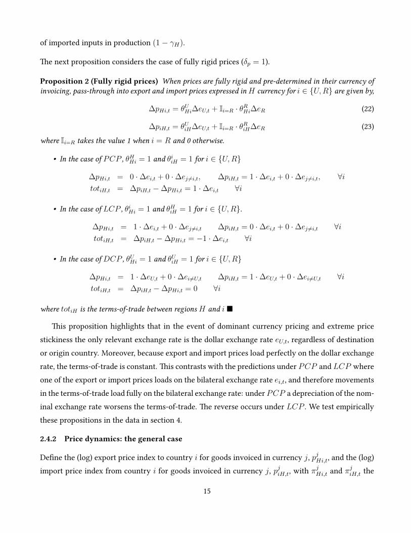


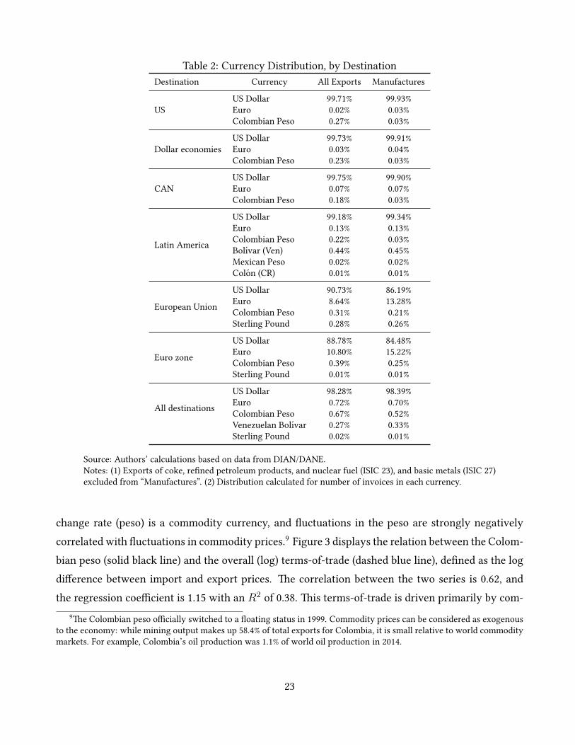


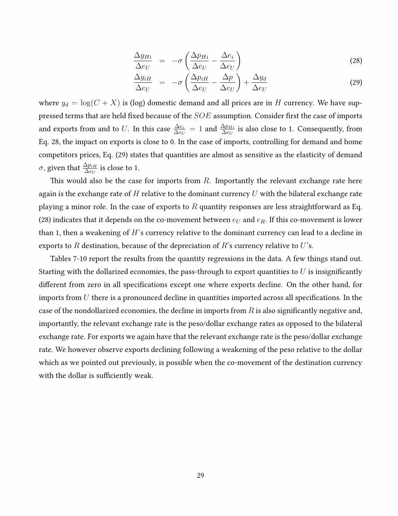

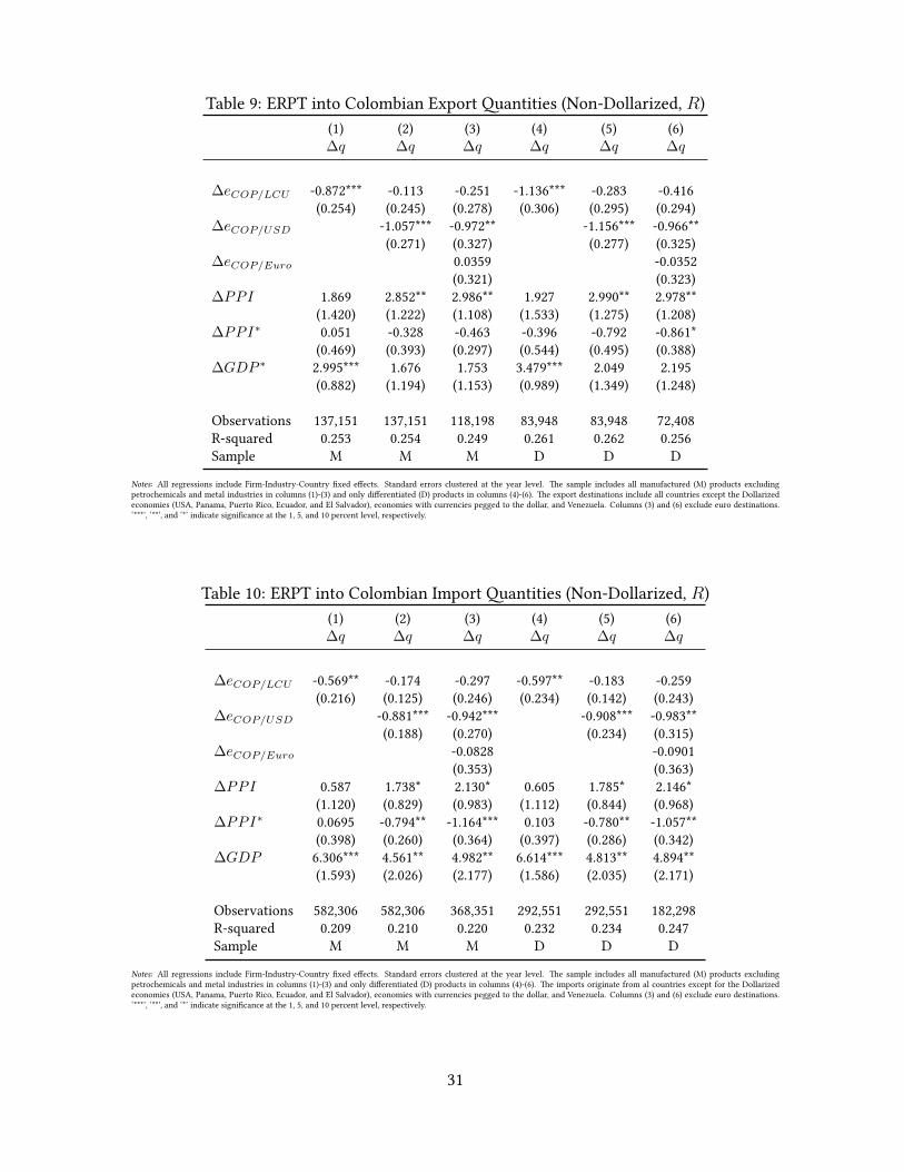


![Integrating Human-Computer Interaction Development into ... · paradigm is typically dominant [Hirschheim and Klein, 1989]. For example, the traditional structured approach is within](https://static.documents.pub/doc/80x56/5e9da1f2111da33d79475d90/integrating-human-computer-interaction-development-into-paradigm-is-typically.jpg)


