Page 1
Munich Personal RePEc Archive
The Environmental cost of Skiing in the
Desert? Evidence from Cointegration
with unknown Structural breaks in UAE
Shahbaz, Muhammad and Sbia, Rashid and Hamdi, Helmi
COMSATS Institute of Information Technology, Lahore, Pakistan,
Free University of Brussels, Central Bank of Bahrain
22 June 2013
Online at https://mpra.ub.uni-muenchen.de/48007/
MPRA Paper No. 48007, posted 05 Jul 2013 04:19 UTC
Page 2
1
The Environmental cost of Skiing in the Desert?
Evidence from Cointegration with unknown Structural breaks in UAE
Muhammad Shahbaz a, b
a Department of Management Sciences,
COMSATS Institute of Information Technology,
Lahore, Pakistan. Email:[email protected]
Cell: +92-334-3664-657, Fax: +92-42-99203100
b School of Social Sciences
National College of Business Administration & Economics
40/E-1, Gulberg III, Lahore-54660, Pakistan
Rashid Sbia*
*Department of Applied Economics
Free University of Brussels
Avenue F. Roosevelt, 50 C.P. 140
B- 1050 Brussels, Belgium
[email protected]
Helmi Hamdi Financial Stability
Central Bank of Bahrain
P.O Box 27, Manama, Bahrain
[email protected]
Abstract: The present study explores the relationship between economic growth, electricity
consumption, urbanization and environmental degradation in case of United Arab Emirates. The
study covers the quarter frequency data over the period of 1975-2011. We have applied the
ARDL bounds testing approach to examine the long run relationship between the variables in the
presence of structural breaks. The VECM Granger causality is applied to investigate the direction
of causal relationship between the variables.
Our empirical exercise reported the existence of cointegration among the series in case of United
Arab Emirates. Further, we found an inverted U-shaped relationship between economic growth
and CO2 emissions i.e. economic growth raises energy emissions initially and declines it after a
threshold point of income per capita (EKC exists). Electricity consumption declines CO2
emissions. The relationship between urbanization and CO2 emissions is positive. Exports seem to
improve the environmental quality by lowering CO2 emissions in case of UAE. The causality
analysis validates the feedback effect between CO2 emissions and electricity consumption.
Economic growth and urbanization Granger cause CO2 emissions.
Keywords: Electricity, Growth, CO2 emissions
Page 3
2
Introduction
The negotiations to extend the Kyoto Protocol which expired in 2012 and to prepare the ground
for future global agreement to replace it are still blocked. This is due mainly to two issues. i)
Developing countries are criticizing the non-commitment of industrialized countries to reduce
their industrial emissions of carbon dioxide and other greenhouse gases. ii) Further, they are
asking more financial aid from the rich nations to poorer countries to move forward for a cleaner
energy source and to reduce greenhouse gases and thus fulfill their pledges under Kyoto
Protocol. Yet, are oil-exporting countries concerned by the latest issue? Mining-resources rich
countries enjoy sizeable revenues coming from oil and gas export. This is case of United Arab
Emirates (UAE).The UAE is a federation of seven emirates namely: Abu Dhabi (the capital
emirate), Ajman, Dubai, Fujairah, Ras-al-Khaimah, Sharjah and Umm al-Quwain. Since early
1960s, when oil was first extracted, the UAE moved from fishing and agricultural-based
economy to an oil-based economy. The UAE is one of the biggest oil producers in the world.
The UAE has observed resilient economic growth in the last decades sustained by high oil prices.
The country has taken advantage to improve its local infrastructure i.e. roads, ports, airports etc.
Developed infrastructure had a direct impact on urbanization. World Urbanization Prospects (the
2011 Revision) reports that the UAE’s urban population jumped from 54.4 % in 1950 to 84.4 %
in 2010. The urbanization rate reached 2.9% over the period of 2005-2010, which is one of the
highest rate in the world. The country’s landscape has changed completely and the UAE has
become one of the most attractive destinations of regional and global tourism. The UAE
government’s ambition went beyond the borders with unique projects including the world’s
Page 4
3
tallest building, artificial island (The Palm and World map), and first shopping mall with indoor
ski-resort (Dubai mall).
However, such development is costly to the environment, as well as to the public health.
Construction industry pollutants are contributing heavily to the air deterioration and water
quality. That is why environmental degradation–economic growth nexus has become one of the
most attractive empirical topics in environmental economics. It has been producing a large
amount literature since the beginning of the 1990s. The major concern of this literature is to
investigate the relationship between income and environmental degradation is also known as
Environmental Kuznets curve (EKC). The EKC hypothesis reveals that environmental
deterioration increases when country witnesses economic growth, but starts to decrease when
income reaches the so-called “turning point”. This hypothesis was first introduced and tested by
Grossman and Krueger, (1991). However, the origins of the EKC are older. In fact, Simon
Kuznets, in his presidential address entitled “Economic Growth and Income Inequality”, in 1955
suggested that as per capita income increases, income inequality increases initially and after a
threshold level of income per capita, income inequality decreases (Kuznets, 1955). This implies
that the relationship between income per capita and income inequality is an inverted U-shaped.
We have chosen to entitled our study “the environmental cost of skiing in the Desert” because
Ski Dubai resort is source of skepticism about its impact on environmental degradation, as it is
an indoor ski slope in the middle of a desert country, where temperature reaches 55° C in the
summer time. Ski Dubai is an indoor ski resort with 22,500 m2. It is within the Mall of the
Emirates, which considered as one of the biggest shopping malls in the world. According to the
Page 5
4
Ski Dubai resort website1, the snow surface is maintained at -16° C and the air temperature is -1°
to -2° during the day. Every night the old snow is moved to be used pre-cool incoming air for the
Mall of the Emirates’ air conditioning system. Exact estimations of energy use for Ski Dubai
could not be found. It is strategic behavior to avoid any kind of criticism. However, some experts
put approximate estimations based on available information and their knowledge2. The average
temperature difference between the inside of the building and the outside is almost 32° C. It is
easy to calculate it given the temperature maintained inside Ski Dubai and the average outdoor
temperature (which can reach 50°). Ski Dubai uses between 525 and 915 Megawatt-hours
(MWh) annually for maintaining its inside temperature, maybe more, depending on the exact
insulation used. Add to this, the heat energy that needs to be removed from water to create snow,
represents at least 700 kWh per day, or 255 MWh per year. Paster, (2010) suggests that Ski
Dubai’s electricity is generated primarily from natural gas, so its annual more than 1000 MWh of
electricity use results in at least 500 tons of greenhouse gas emissions. He makes an interesting
representation of the annual greenhouse gas emissions of Ski Dubai. He advances that they are
equivalent to about 900 round-trip flights from Dubai to Munich (561 kg per person, per round
trip). This make easy to target Ski Dubai as a model of waste and excess.
II. Literature Review
In pioneering effort, Grossman and Krueger, (1991) used the Kuznets curve as a tool to analyze
the relationship between the environmental degradation and income per capita. It is important to
mention that there is no convention on the best indicator to be used for environmental
degradation. Some researchers use carbon dioxide emissions (Holtz-Eakinand and Selden, 1992;
1 See www.theplaymania.com/skidubai 2See Pablo Paster, 2010 on www.treehugger.com/clean-technology/ask-pablo-indoor-skiing-really -that-bad.html.
Page 6
5
Roberts and Grimes, 1997; Moomaw and Unruh, 1997 and among others) and other use sulfur
dioxide emissions (Grossman and Krueger, 1991; Panayotou, 1997; Davidsdottir et al. 1998 and
among others). A bulky amount of studies tested the economic growth and environmental
pollution nexus. However, this literature could be divided to two distinguished components. The
first component investigates the pollution–economic growth nexus for across-section and/or
panel of countries. The second component investigates for individual countries. As it is
impossible to review all studies due its large amount, we would review some of recent selected
examples from both single studies and cross-sectional/panel data-based analysis of the EKC
hypothesis.
In panel framework, Holtz-Eakin and Selden, (1995) estimated a quadratic polynomial model on
the panel of 130 countries over the period of 1951-1986 and supported the EKC hypothesis.
Similarly; Tucker, (1995) examined the EKC hypothesis using CO2 emissions as an indicator of
environmental degradation using cross-section data of 131 countries and results supported for
EKC hypothesis. Cole et al. (1997) used wide range of indictors (Nitrogen dioxide, Sulphur
dioxide, Suspended particulate matter, Carbon monoxide, Nitrogen dioxide from transport,
Sulphur dioxide from transport, SPM from transport, Nitrate concentrations, Carbon dioxide,
Total energy use, CFCs and halons, Methane, Municipal waste, Energy use from transport,
Traffic volumes) to investigate the relationship between economic growth and environmental
degradation. They employed a quadratic polynomial model using both linear and log-linear
versions. Their empirical analysis advocated that the EKC hypothesis exists only for local air
pollutants. Hill and Magnani, (2002) argued that the EKC for carbon emissions is found to be
highly sensitive to the dataset used. They used data for 156 countries and examined the KEC
Page 7
6
hypothesis for 1970, 1980 and 1990. Their empirical exercised showed the EKC hypothesis for
three cross-sections.
Recently; Apergis and Payne, (2009) examined the relationship between energy consumption,
CO2 emissions and economic growth for six Central American economies using the panel
VECM. They reported that energy consumption raises CO2 emissions and relationship between
CO2 emissions and economic growth in an inverted U-shaped i.e. KEC is confirmed. Narayan
and Narayan, (2010) collected the data of 43 developing economies to examine whether EKC
exist or not. Based on individual country analysis, they reported that in approximately 35 percent
of the sample carbon dioxide emissions have fallen over the long run. Moreover, their results
indicated that only for the Middle Eastern and South Asian panels, the income elasticity in the
long run is smaller than the short run, implying that carbon dioxide emission has fallen with rise
in income. For panel of BRIC countries; Pao and Tsai, (2010) investigated the dynamic causal
relationships between pollutant emissions, energy consumption and economic growth. They
found the long run relationship between the series. Energy consumption has positive impact on
energy emissions and the EKC hypothesis also exists in BRIC region. The panel causality
analysis revealed the feedback effect between energy consumption and CO2 emissions and same
is true for economic growth and energy consumption. They suggested that in order to reduce CO2
emissions and not to adversely affect economic growth, increasing both energy supply
investment and energy efficiency, and speeding up energy conservation policies to reduce
wastage of energy can be initiated for energy-dependent BRIC countries.
Page 8
7
Jaunky, (2011) attempted to test the environment Kuznets curve (EKC) hypothesis for 36 high-
income countries following Narayan and Narayan, (2010). Based on single country analysis,
results found inverted U-shaped relationship between economic growth and CO2 emissions i.e.
EKC only in Greece, Malta, Oman, Portugal and the United Kingdom. Piaggio and Padilla,
(2012) explored the relationship between CO2 emissions and economic growth for 31 countries
(28 OECD, Brazil, China, and India). They confirmed the necessity relevance of considering the
differences among countries in the relationship between air pollution and economic activity to
avoid wrong estimations and conclusions. Arouri et al. (2012) investigated whether the
relationship between economic growth and CO2 emissions shows EKC phenomenon or not by
applying bootstrap panel unit root tests and cointegration techniques. Their results showed that
energy consumption is a major contributor to CO2 emissions. However, the EKC hypothesis is
confirmed in the long run in most sample countries, the turning points are very low in some cases
and very high in other cases. This could reduce the evidence supporting of the EKC hypothesis.
They suggested that future reductions in CO2 emissions per capita might be achieved at the same
time as GDP per capita in the MENA region continues to grow.
De Bruyn et al. (1998) argued that the estimation of the EKC from panel data cannot capture the
dynamics of the relationship between income and emissions and policy implications from panel
data analysis could not be helpful for single country. To overcome this issue, time series single
country analysis must be conducted. Later on, Roca et al. (2001) used six indicators of
environmental degradation in case of Spain to examine the existence of EKC hypothesis between
emissions and economic growth. They only found inverted U-shaped relationship between SO2
emissions and economic growth. However, Lindmark, (2002) reported that time-specific
Page 9
8
technological advancements may affect the relationship between economic growth and emissions
in Swedish economy. In case of Austria, Friedl and Getzner, (2003) explored the relationship
between economic growth and energy pollutants to test the either EKC hypothesis exists or not
over the period of 1960-1999. They did not find inverted U-shaped or U-shaped but cubic i.e. N-
shaped relationship between economic growth and CO2 emissions.
Lantz and Feng, (2006) incorporated population and technology in emissions function to
examine the relationship between economic growth and emissions over the period of 1970-2000
in case of Canada. They noted that did not find any evidence on relationship between economic
growth and emissions but incorporation of population and technology supported for inverted U-
shaped and U-shaped relationship between economic growth and emissions. He and Richard,
(2010) also found the little evidence about the existence of KEC hypothesis between economic
growth and CO2 emissions. In case of French economy, Ang (2007) investigated the relationship
between economic growth and CO2 emissions by incorporating energy consumption in
multivariate framework. He found long run relationship among the series but could not find
evidence on EKC hypothesis and economic growth Granger causes energy consumption and CO2
emissions in long run. In US economy, Soytas et al. (2007) examined the existence of inverted
U-shaped relationship economic growth and CO2 emissions by incorporating energy
consumption, gross fixed capital formation and labor. They failed to find empirical evidence of
EKC hypothesis but unidirectional causality is found running from economic growth to energy
consumption.
Page 10
9
Ang (2008) used same idea for Malaysian economy to examine whether KEC hypothesis does
exit or not. He noted that the variables are cointegrated for long run relationships and energy
consumption is Granger cause of economic growth. On contrary, Saboori et al. (2012)
scrutinized the validation of EKC hypothesis by incorporating trade openness in CO2 emissions
function. They found long run relationship between the variables and existence of EKC in
Malaysia. The VECM Granger causality analysis found that CO2 emissions are Granger cause of
economic growth in long run but in short run, feedback effect exists between economic growth
and CO2 emissions.
Chebbi, (2009) applied the Johansen cointegration for long run and the VECM Granger causality
test for causal relationships. He found cointegration between the variables but failed to find EKC
hypothesis. The VECM Granger causality analysis revealed that economic growth is Granger
cause CO2 emissions and economic growth Granger causes energy consumption. Halicioglu,
(2009) examined the impact of determinants of CO2 emissions in case of Turkey and reported
long run relationship among economic growth, energy consumption, international trade and CO2
emissions. He found positive impact of energy consumption and trade openness and inverted U-
shaped i.e. EKC hypothesis between economic growth and CO2 emissions. Later on, Ozturk, and
Acaravci, (2010) applied trivariate model to investigate the relationship between energy
consumption, economic growth and CO2 emissions and found no evidence of environmental
Kuznets curve in Turkey. They reported neutral effect among energy consumption, economic
growth and CO2 emissions. In case of Chinese economy; Jalil and Mahmud, (2009) investigated
whether environmental Kuznets curve (EKC) relationship between CO2 emissions and per capita
real GDP holds in long-run or not in the presence of trade openness. The ARDL bounds testing
Page 11
10
approach is applied for long run. Their results showed a quadratic relationship between income
and CO2 emissions supporting EKC hypothesis. They further reported that economic growth
Granger causes CO2 emissions. But Kareem et al. (2012) examined the impact of energy
consumption, economic growth, trade openness and capitalization on CO2 emissions. They
reported that the said variables contribute to CO2 emissions but could not validate the findings of
Jalil and Mahmud, (2009). Similarly, Shuang-Ying and Wen-Cong, (2011) applied bivariate
model to examine relationship between economic growth and energy consumption but failed to
find environmental Kuznets curve (EKC) empirically in Zhejiang province of China.
Iwata et al. (2010) investigated the existence of EKC hypothesis by incorporating nuclear energy
consumption in CO2 emissions function in case of France. They found long run relationship
among economic growth, nuclear energy consumption and CO2 emissions. Their empirical
exercise validated that relationship between economic growth and CO2 emissions is inverted U-
shaped i.e. EKC effect exits and nuclear energy consumption lowers CO2 emissions. Seetanah
and Vinesh, (2010) used Mauritius data to investigate the nature of relationship between
economic growth and CO2 emissions by incorporating investment, trade openness, education and
employment using multivariate framework. They reported that trade openness, economic growth
and employment increase CO2 emissions but education declines it. Their empirical exercise
could provide support for the EKC hypothesis. Shanthini and Perera, (2011) investigated the
cointegration between economic growth and CO2 emissions in case of Australia. Their results
indicated the long run relationship between the series but could evidence about the EKC
hypothesis. They noted negative impact of economic growth on CO2 emissions in short run as
well as in long run.
Page 12
11
Pao et al. (2011) applied the cointegration and causality approaches to examine the dynamic
relationships between pollutant emissions and real output in case of Russia. Their results found
inverse impact of real output on CO2 emissions which does not present the support for EKC
hypothesis. Their causality analysis revealed the feedback effect real output and CO2 emissions.
This suggests that to reduce emissions, the best environmental policy is to increase infrastructure
investment to improve energy efficiency, and to step up energy conservation policies to reduce
any unnecessary waste of energy. That is, energy conservation is expected to improve energy
efficiency, thereby promoting economic growth. Saboori et al. (2011) investigated whether EKC
exists or not in the presence of trade openness in Indonesia. Their findings found that
relationship between economic growth and CO2 emissions are inverted-U shaped. But, Hwang
and Yoo, (2012) failed to validate the findings reported by Saboori et al. (2011) and reported
energy consumption and CO2 emissions are Granger cause of economic growth. Hossain, (2012)
incorporated urbanization and trade openness to investigate the relationship between economic
growth and CO2 emissions in case of Japan. The empirical results found cointegration among the
series and energy consumption, economic growth and urbanization are major contributors to CO2
emissions while trade openness improves environmental quality by lowering CO2 emissions.
Hossain, (2012) could not provide empirical support for KEC effect for Japan. In case of Spain,
Esteve and Tamarit (2012) empirically investigated the relationship between economic growth
and CO2 emissions by applying threshold cointegration over the period of 1857-2007. Their
results confirmed the non-linear relationship between economic growth and CO2 emissions
supporting the EKC hypothesis.
Page 13
12
In case of India, Tiwari (2011) examined the relationship between total primary energy
consumption, economic growth and CO2 emissions. He found long run relationship among the
series and economic growth Granger causes energy consumption but neutral effect exists
between economic growth and CO2 emissions while same is true for energy consumption and
CO2 emissions. Then, Tiwari et al. (2013) incorporated coal consumption in CO2 emissions
function to examine the EKC hypothesis in case of India. Their results confirmed the existence
of long run relationship as well as the EKC hypothesis. The VECM causality analysis revealed
the feedback hypothesis between economic growth and CO2 emissions. The bidirectional
causality was found between coal consumption and CO2 emissions. Moreover, trade openness
Granger causes economic growth, coal consumption and CO2emissions. Later on, Kanjilal and
Ghosh (2013) validated the findings of Tiwari et al. (2013) and reported the negative impact of
trade openness on CO2emissions. In case of Pakistan, Shahbaz et al. (2012) investigated the
relationship between CO2 emissions, energy consumption, economic growth and trade openness
to examine whether the EKC exists or not. Their results supported the existence of the
environmental Kuznets curve (EKC) hypothesis. The causality analysis revealed that CO2
emissions are Granger cause of economic growth and energy consumption. Ahmed and Long,
(2012) confirmed the findings reported by Shahbaz et al (2012) and found positive impact of
energy consumption, exports and population growth on CO2 emissions. In case of Romania,
Shahbaz et al. (2013) probed the existence of EKC hypothesis over the period of 1980-2010.
They applied the ARDL bounds testing for long run and reported that relationship between
economic growth and CO2 emissions is inverted U-shaped i.e. the EKC hypothesis is found.
Furthermore, energy consumption contributes to CO2 emissions significantly and democracy is
negative linked with CO2 emissions due to effective adoption of economic and financial policies.
Page 14
13
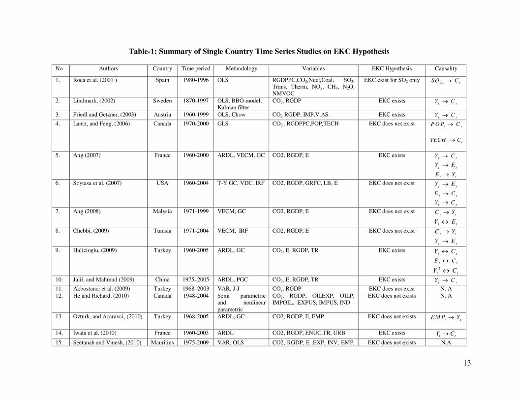
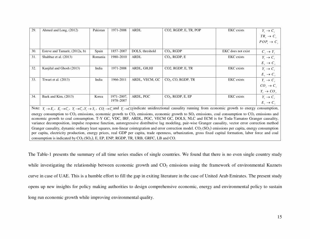
Table-1: Summary of Single Country Time Series Studies on EKC Hypothesis
No Authors Country Time period Methodology Variables EKC Hypothesis Causality
1. Roca et al. (2001 ) Spain 1980-1996 OLS RGDPPC,CO2,Nucl,Coal, SO2, Trans, Therm, NOx, CH4, N2O, NMVOC
EKC exist for SO2 only 2 t t
SO C
2. Lindmark, (2002) Sweden 1870-1997 OLS, BBO-model, Kalman filter
CO2, RGDP EKC exists tt
CY
3. Friedl and Getzner, (2003) Austria 1960-1999 OLS, Chow CO2, RGDP, IMP,V.AS EKC exists tt
CY
4. Lantz, and Feng, (2006) Canada 1970-2000 GLS CO2,, RGDPPC,POP,TECH EKC does not exist t t
P O P C
t tTECH C
5. Ang (2007) France 1960-2000 ARDL, VECM, GC CO2, RGDP, E EKC exists tt
CY
ttEY
t tE Y
6. Soytasa et al. (2007) USA 1960-2004 T-Y GC, VDC, IRF CO2, RGDP, GRFC, LB, E EKC does not exist tt
EY
ttCE
tt CY
7. Ang (2008) Malysia 1971-1999 VECM, GC CO2, RGDP, E EKC does not exist t t
C Y
t tY E
8. Chebbi, (2009) Tunisia 1971-2004 VECM, IRF CO2, RGDP, E EKC does not exist t t
C Y
ttEY
9. Halicioglu, (2009) Turkey 1960-2005 ARDL, GC CO2, E, RGDP, TR EKC exists t t
Y C
t tE C
2
t tY C
10. Jalil, and Mahmud (2009) China 1975–2005 ARDL, PGC CO2, E, RGDP, TR EKC exists tt
CY
11. Akbostanci et al. (2009) Turkey 1968–2003 VAR, J-J CO2, RGDP EKC does not exist N. A
12. He and Richard, (2010) Canada 1948-2004 Semi parametric and nonlinear
parametric
CO2, RGDP, OILEXP, OILP, IMPOIL, EXPUS, IMPUS, IND
EKC does not exists N. A
13. Ozturk, and Acaravci, (2010) Turkey 1968-2005 ARDL, GC CO2, RGDP, E, EMP EKC does not exists t t
EM P Y
14. Iwata et al. (2010) France 1960-2003 ARDL CO2, RGDP, ENUC,TR, URB EKC exists tt CY
15. Seetanah and Vinesh, (2010) Mauritius 1975-2009 VAR, OLS CO2, RGDP, E ,EXP, INV, EMP, EKC does not exists N.A
Page 15
14
EDUC
16. Iwata et al. (2010) France 1960-2003 ARDL, VECM, GC CO2, RGDP, EP, TR, E, URB EKC exists tt CY
tt CE
17. Fodha, and Zaghdoud,(2010) Tunisia 1961–2004 VECM, GC CO2, SO2, RGDP EKC exists tt
SY
tt CY
18. Pao, etal.(2011) Russia 1990-2007 VECM, GC CO2, E, RGDP EKC does not exist tt EY
tt CE
ttCY
19. Saboori et al. (2011) Malaysia 1980-2009 ARDL,VECM, GC CO2, RGDP EKC exists tt CY
20. Shuang-Ying and Wen-Cong, (2011)
Zhejiang province
1990-2009 OLS LOA, RGDP EKC does not exist N.A
21. Shanthini and Perera, (2011) Australia 1960-2009 ARDL CO2, RGDP,OILP EKC exists tt CY
22. Tiwari (2011) India 1971-2007 VAR,GC,IRF CO2, E, RGDP, GFCF, POP EKC does not exist tt CE
t tE Y
23. Fosten et al. (2012) UK 1830-2003 NLC, ECM CO2, SO2, RGDP, ENP EKC exists tt
SY
tt CY
24. Saboori et al. (2012) Malaysia 1980-2009 ARDL, GC CO2, RGDP EKC exists tt
CY
25. Shahbaz et al. (2012) Pakistan 1971–2009 ARDL, PGC CO2, E, RGDP, TR EKC exists tt CY
tt CE
26. Kareem et al. (2012) China 1971-2008 VECM, GC CO2, E, RGDP, GFCF, GEXP,
IND
EKC does not exist t t
C Y
t tY E
t tIND C
27. Hwang and Yoo, (2012) Indonesia 1965-2006 VECM, GC CO2, RGDP, E, EKC exists tt CY
t tY E
t tE C
28. Hossain, (2012) Japan 1960-2009 ARDL,VECM, GC CO2, RGDP, E, TR, URB EKC does not exist tt CE
t tTR C
tt CY
Page 16
15
29. Ahmed and Long, (2012) Pakistan 1971-2008 ARDL CO2, RGDP, E, TR, POP EKC exists tt CY
t tTR C
t tPOP C
30. Esteve and Tamarit, (2012a, b) Spain 1857–2007 DOLS, threshold CO2, RGDP EKC does not exist t t
C Y
31. Shahbaz et al. (2013) Romania 1980–2010 ARDL CO2, RGDP, E EKC exists tt CY
tt CE
32. Kanjilal and Ghosh (2013) India 1971-2008 ARDL, GH,HJ CO2, RGDP, E, TR EKC exists tt CY
tt CE
33. Tiwari et al. (2013) India 1966-2011 ARDL, VECM, GC CO2, CO, RGDP, TR EKC exists tt CY
tt CCO
tt COY
34. Baek and Kim, (2013) Korea 1971–2007, 1978–2007
ARDL, PGC CO2, RGDP, E, EP EKC exists tt CY
tt CE
Note: tt EY ,
tt CE , tt CY ,
tt SY , tt CCO and
tt COY indicate unidirectional causality running from economic growth to energy consumption,
energy consumption to CO2 emissions, economic growth to CO2 emissions, economic growth to SO2 emissions, coal consumption to CO2 emissions and
economic growth to coal consumption. T-Y GC, VDC, IRF, ARDL, PGC, VECM GC, DOLS, NLC and ECM is for Toda-Yamatoo Granger causality,
variance decomposition, impulse response function, autoregressive distributive lag modeling, pair-wise Granger causality, vector error correction method
Granger causality, dynamic ordinary least squares, non-linear cointegration and error correction model. CO2 (SO2) emissions per capita, energy consumption
per capita, electricity production, energy prices, real GDP per capita, trade openness, urbanization, gross fixed capital formation, labor force and coal
consumption is indicated by CO2 (SO2), E, EP, ENP, RGDP, TR, URB, GRFC, LB and CO.
The Table-1 presents the summary of all time series studies of single countries. We found that there is no even single country study
while investigating the relationship between economic growth and CO2 emissions using the framework of environmental Kuznets
curve in case of UAE. This is a humble effort to fill the gap in exiting literature in the case of United Arab Emirates. The present study
opens up new insights for policy making authorities to design comprehensive economic, energy and environmental policy to sustain
long run economic growth while improving environmental quality.
Page 17
16
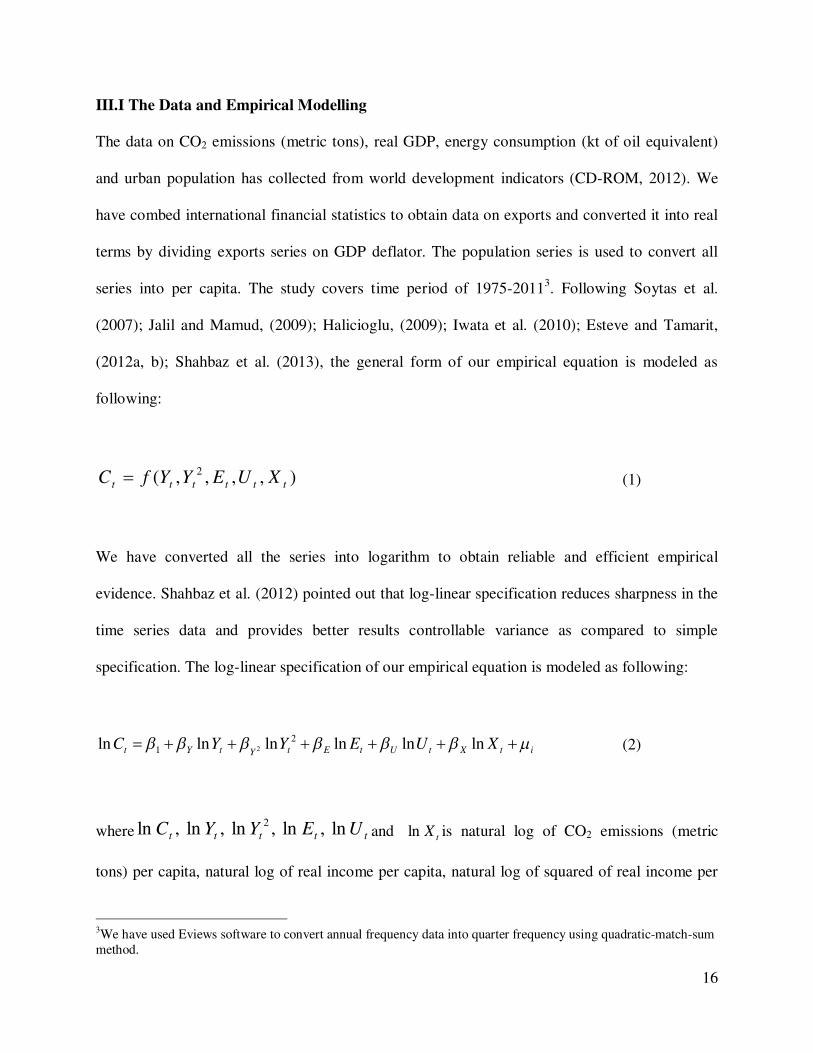
III.I The Data and Empirical Modelling
The data on CO2 emissions (metric tons), real GDP, energy consumption (kt of oil equivalent)
and urban population has collected from world development indicators (CD-ROM, 2012). We
have combed international financial statistics to obtain data on exports and converted it into real
terms by dividing exports series on GDP deflator. The population series is used to convert all
series into per capita. The study covers time period of 1975-20113. Following Soytas et al.
(2007); Jalil and Mamud, (2009); Halicioglu, (2009); Iwata et al. (2010); Esteve and Tamarit,
(2012a, b); Shahbaz et al. (2013), the general form of our empirical equation is modeled as
following:
),,,,( 2
tttttt XUEYYfC (1)
We have converted all the series into logarithm to obtain reliable and efficient empirical
evidence. Shahbaz et al. (2012) pointed out that log-linear specification reduces sharpness in the
time series data and provides better results controllable variance as compared to simple
specification. The log-linear specification of our empirical equation is modeled as following:
itXtUtEtYtYt XUEYYC lnlnlnlnlnln 2
1 2 (2)
where ttttt UEYYC ln,ln,ln,ln,ln 2and tXln is natural log of CO2 emissions (metric
tons) per capita, natural log of real income per capita, natural log of squared of real income per
3We have used Eviews software to convert annual frequency data into quarter frequency using quadratic-match-sum
method.
Page 18
17
capita, energy consumption (kt of oil equivalent) per capita, urbanization per capita and real
exports per capita. i is error term with constant variance and zero mean and having normal
distribution. We expect inverted U-shaped i.e. EKC hypothesis between economic growth and
CO2 emissions if 0Y and 02 Y
otherwise U-shaped relationship exist. The 0E
implies that efficient use of energy lowers CO2 emissions otherwise energy consumption
degrades environmental quality if 0E . We can expect positive or negative impact of
urbanization on CO2 emissions. If urbanization is planned and urban population has easy access
to energy efficient technology such as consumer durables for consumers and advanced
technology for producers then 0U otherwise 0E . The impact of exports on CO2
emissions depends upon the technology to be implemented in an economy if an economy uses
energy efficient technology then 0X otherwise an increase in exports will raise CO2
emissions i.e. 0x .
III.II Zivot-Andrews Unit Root Test
The usual first step in empirical analysis is to test the stationarity properties of the variables.
Traditional unit root tests are ADF by Dickey and Fuller (1979), P-P by Philips and Perron
(1988), KPSS by Kwiatkowski et al. (1992), DF-GLS by Elliott et al. (1996) and Ng-Perron by
Ng-Perron (2001). However, as pointed by Baum, (2004), empirical evidence on order of
integration of the variable by ADF, P-P and DF-GLS unit root tests are not reliable in the
presence of structural break in the series. In fact, unit root tests may be biased and inappropriate
in absence of information about structural break occurred in series.
Page 19
18
To overcome this problem, Zivot-Andrews (1992) suggested three models to test the stationarity
properties of the variables in the presence of structural break point in the series. (i) First model
permits a one-time change in variables at level form, (ii) second model allows a one-time change
in the slope of the trend component i.e. function and (iii) last model has one-time change both in
intercept and trend function of the variables to be used in the analysis. Zivot-Andrews, (1992)
adopted three models to check the hypothesis of one-time structural break in the series as
follows:
k
j
tjtjtttxdcDUbtaxax
1
1 (3)
k
j
tjtjtttxdbDTctbxbx
1
1 (4)
k
j
tjtjttttxddDTdDUctcxcx
1
1 (5)
where tDU represents the dummy variables displaying mean shift occurred at each point with
time break while trend shift variables is presented by tDT 4. So,
TBtif
TBtifDU t
...0
...1and
TBtif
TBtifTBtDU t
...0
...
The null hypothesis of unit root break date is 0c which indicates that series is not stationary
with a drift not having information about structural break point while 0c hypothesis implies
that the variable is found to be trend-stationary with one unknown time break. Zivot-Andrews
unit root test fixes all points as potential for possible time break and does estimation through
4We used model-4 for empirical estimations following Sen, (2003)
Page 20
19
regression for all possible break points successively. After that, this unit root test selects that
time break which decreases one-sided t-statistic to test 1)1(ˆ cc . Zivot-Andrews indicate
that in the presence of end-points, asymptotic distribution of the statistics is diverged to infinity
point. It is compulsory to choose a region where end-points of sample period are excluded. To do
so, we followed Zivot-Andrews suggestions by choosing the trimming regions i.e. (0.15T,
0.85T).
III.II The ARDL Bounds Testing
We employ the autoregressive distributed lag (ARDL) bounds testing approach to cointegration
developed by Pesaran et al. (2001) to explore the existence of long run relationship between
economic growth, electricity consumption, urbanization, exports and CO2 emissions in the
presence of structural break. This approach has multiple econometric advantages. The bounds
testing approach is applicable irrespective of whether variables are I(0) or I(1). Moreover, a
dynamic unrestricted error correction model (UECM) can be derived from the ARDL bounds
testing through a simple linear transformation. The UECM integrates the short run dynamics
with the long run equilibrium without losing any long run information. The UECM is expressed
as follows:
tD
t
m
mtm
s
l
ltl
r
k
ktk
q
j
jtj
p
i
ititUtXtEtYtCTt
DUXEY
CUXEYCTC
1
0000
1
111111
lnlnlnln
ln lnlnlnlnlnln
(6)
Page 21
20
tD
t
m
mtm
s
l
ltl
r
k
ktk
q
j
jtj
p
i
ititUtXtEtYtCTt
DUXEC
YUXEYCTY
2
0000
1
111111
lnlnlnln
lnlnlnlnlnlnln
(7)
tD
t
m
mtm
s
l
ltl
r
k
ktk
q
j
jtj
p
i
ititUtXtEtYtCTt
DUXCY
EUXEYCTE
3
0000
1
111111
lnlnlnln
lnlnlnlnlnlnln
(8)
tD
t
m
mtm
s
l
ltl
r
k
ktk
q
j
jtj
p
i
ititUtXtEtYtCTt
DUEYC
XUXEYCTX
4
0000
1
111111
lnlnlnln
lnlnlnlnlnlnln
(9)
tD
t
m
mtm
s
l
ltl
r
k
ktk
q
j
jtj
p
i
ititUtXtEtYtCTt
DXEYC
UUXEYCTU
5
0000
1
111111
lnlnlnln
lnlnlnlnlnlnln
(10)
where Δ is the first difference operator, D is dummy for structural break point based on Z-A test
and t is error term assumed to be independently and identically distributed. The optimal lag
structure of the first differenced regression is selected by the Akaike information criteria (AIC).
Pesaran et al. (2001) suggest F-test for joint significance of the coefficients of the lagged level of
variables. For example, the null hypothesis of no long run relationship between the variables is
0:0 UXEYCH against the alternative hypothesis of cointegration
0: UXEYCaH . Pesaran et al. (2001) computed two set of critical value (lower
and upper critical bounds) for a given significance level. Lower critical bound is applied if the
regressors are I(0) and the upper critical bound is used for I(1). If the F-statistic exceeds the
upper critical value, we conclude in favor of a long run relationship. If the F-statistic falls below
Page 22
21
the lower critical bound, we cannot reject the null hypothesis of no cointegration. However, if the
F-statistic lies between the lower and upper critical bounds, inference would be inconclusive.
When the order of integration of all the series is known to be I(1) then decision is made based on
the upper critical bound. Similarly, if all the series are I(0), then the decision is made based on
the lower critical bound. To check the robustness of the ARDL model, we apply diagnostic tests.
The diagnostics tests are checking for normality of error term, serial correlation, autoregressive
conditional heteroskedasticity, white heteroskedasticity and the functional form of empirical
model.
III.III The VECM Granger Causality
After examining the long run relationship between the variables, we use the Granger causality
test to determine the causality between the variables. If there is cointegration between the series
then the vector error correction method (VECM) can be developed as follows:
t
t
t
t
t
t
t
t
t
t
t
mmmmm
mmmmm
mmmmm
mmmmm
mmmmm
t
t
t
t
t
t
t
t
t
t
ECM
U
X
E
Y
C
BBBBB
BBBBB
BBBBB
BBBBB
BBBBB
U
X
E
Y
C
BBBBB
BBBBB
BBBBB
BBBBB
BBBBB
b
b
b
b
U
X
E
Y
C
5
4
3
2
1
1
5
4
3
3
1
1
1
1
1
1
,55,54,53,52,51
,45,44,43,42,41
,35,34,33,32,31
,25,24,23,22,21
,15,14,13,12,11
1
1
1
1
1
1,451,441,431,421,41
1,451,441,431,421,41
1,351,341,331,321,31
1,251,241,231,221,21
1,151,141,131,121,11
4
3
2
1
)(
ln
ln
ln
ln
ln
...
ln
ln
ln
ln
ln
ln
ln
ln
ln
ln
(11)
Page 23
22
where difference operator is and 1tECM is the lagged error correction term, generated from
the long run association. The long run causality is found by significance of coefficient of lagged
error correction term using t-test statistic. The existence of a significant relationship in first
differences of the variables provides evidence on the direction of short run causality. The joint
2 statistic for the first differenced lagged independent variables is used to test the direction of
short-run causality between the variables. For example, iiB 0,12 shows that economic growth
Granger causes CO2 emissions and economic growth is Granger of cause of CO2 emissions if
iiB 0,11 .
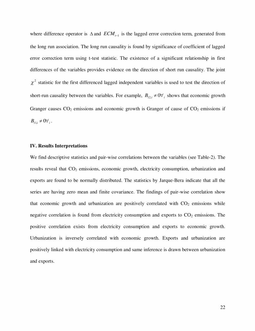
IV. Results Interpretations
We find descriptive statistics and pair-wise correlations between the variables (see Table-2). The
results reveal that CO2 emissions, economic growth, electricity consumption, urbanization and
exports are found to be normally distributed. The statistics by Jarque-Bera indicate that all the
series are having zero mean and finite covariance. The findings of pair-wise correlation show
that economic growth and urbanization are positively correlated with CO2 emissions while
negative correlation is found from electricity consumption and exports to CO2 emissions. The
positive correlation exists from electricity consumption and exports to economic growth.
Urbanization is inversely correlated with economic growth. Exports and urbanization are
positively linked with electricity consumption and same inference is drawn between urbanization
and exports.
Page 24
23
Table-2: Descriptive Statistics and Correlation Matrix
Variable tCln tYln tEln tUln tXln
Mean 3.4406 12.3273 9.0609 4.3876 8.3744
Median 3.4293 12.2620 9.1399 4.3826 8.3115
Maximum 4.1511 12.8449 9.5342 4.4355 9.2260
Minimum 2.7692 11.5962 7.7773 4.3607 7.7646
Std. Dev. 0.2863 0.2919 0.4321 0.0201 0.3835
Skewness 0.3600 -0.0706 -1.3198 0.9095 0.5170
Kurtosis 4.1451 2.9880 4.3433 2.8811 2.4247
Jarque-Bera 2.8212 0.0309 3.5247 5.1229 2.1590
Probability 0.2439 0.9846 0.1100 0.0771 0.3397
tCln 1.0000
tYln 0.6726 1.0000
tEln -0.7574 0.7267 1.0000
tUln 0.2205 -0.4709 0.3299 1.0000
tXln -0.3975 0.4582 0.4584 0.0812 1.0000
The assumption of the ARDL bounds testing is that the series should be integrated at I(0) or I(1)
or I(0) / I(1). This implies that the none of variables is integrated at I(2). To resolve this issue, we
have applied traditional unit root tests such as ADF, PP and DF-GLS5. Our empirical exercise
finds that CO2 emissions ( tCln ), electricity consumption ( tEln ), economic growth ( tYln ),
5Results are available upon request from authors
Page 25
24
exports ( tXln ) and urbanization ( tUln ) are not found to be stationary at level with constant and
trend. This shows that the variables are integrated at I(1). The main issue with these unit tests is
that these tests do not seem to consider information about unknown structural beaks in the series.
This implies that traditional unit root tests provide ambiguous results regarding integrating
properties of the variables. The appropriate information about structural break would help policy
makers in designing inclusive energy, economic, urban and trade policy to sustain environmental
quality in long run. We have applied Zivot-Andrews unit root test which accommodates single
unknown structural break in the variables.
Table-3: Zivot-Andrews Structural Break Unit Root Test
Variable At Level At 1st Difference
T-statistic Time Break T-statistic Time Break
tCln -3.285 (2) 1999Q2 -9.170 (4)* 1997Q3
tYln -2.551 (5) 2000Q2 -7.632 (2)* 1988Q2
tEln -4.503 (3) 1997Q4 -8.277 (0)* 1992Q2
tUln -4.962 (5) 1995Q3 -7.943 (0)* 1995Q2
tXln -4.384 (4) 1982Q1 -8.359 (0)* 1980Q3
Note: * represent significant at 1% level of significance. The critical
value at1% is -5.57 and at 5% is -5.08. Lag order is shown in
parenthesis.
Page 26
25
The results are detailed in Table-3. We find, while applying Zivot-Andrews, (1992) test with
single unknown break, that economic growth, electricity consumption, exports, urbanization and
CO2 emissions have unit root at level with intercept and trend. The structural breaks are found in
economic growth, electricity consumption, exports, urbanization and CO2 emissions in 2000Q2,
1997Q4, 1982Q1, 1995Q3 and 1999Q2 respectively. The variables are found to be stationary at
1st difference. This implies that series have same level of integration. The robustness of results is
validated by applying Zivot-Andrews, (1992) with single unknown structural break. Our findings
indicate that variables are integrated at I(1). The unique integrating order of the variables lends a
support to test the existence of cointegration between the variables. In doing so, we apply the
ARDL bounds testing approach in the presence of structural break to examine cointegration
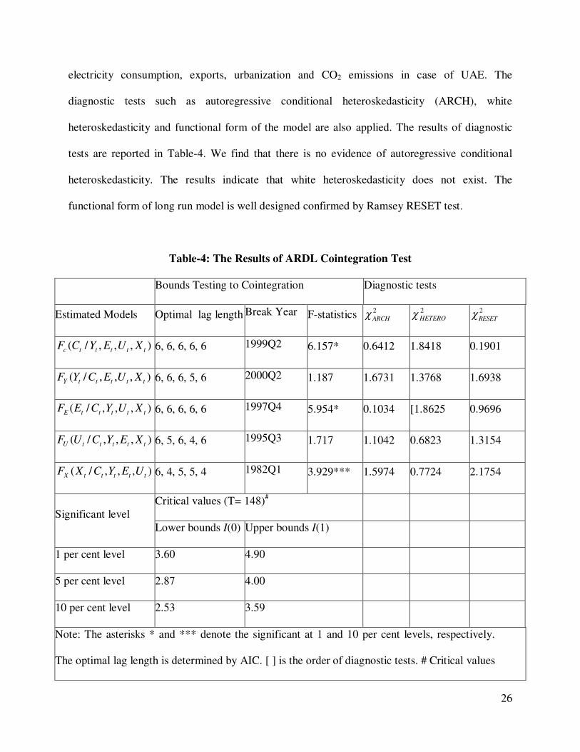
between the variables. The results are reported in Table-4. The lag order of the variable is chosen
following Akaike information criterion (AIC) due to its superiority over Schwartz Bayesian
criterion (SBC). AIC performs relatively well in small samples but is inconsistent and does not
improve performance in large samples whilst SBC in contrast appears to perform relatively
poorly in small samples but is consistent and improves in performance with sample size
(Acquah, 2010).
The appropriate lag section is required because F-statistic variables with lag order of the
variables. The lag order of the variables is given in second column of Table-4. The results
reported in Table-4 reveal that our computed F-statistics are greater than upper critical bounds
generated by Pesaran et al. (2001) which are suitable for small data set. We find three
cointegrating vectors once CO2 emissions, electricity consumption and exports are used as
dependent actors. This validates that there is long run relationship between economic growth,
Page 27
26
electricity consumption, exports, urbanization and CO2 emissions in case of UAE. The
diagnostic tests such as autoregressive conditional heteroskedasticity (ARCH), white
heteroskedasticity and functional form of the model are also applied. The results of diagnostic
tests are reported in Table-4. We find that there is no evidence of autoregressive conditional
heteroskedasticity. The results indicate that white heteroskedasticity does not exist. The
functional form of long run model is well designed confirmed by Ramsey RESET test.
Table-4: The Results of ARDL Cointegration Test
Bounds Testing to Cointegration Diagnostic tests
Estimated Models Optimal lag length Break Year F-statistics 2
ARCH
2
HETERO 2
RESET
),,,/( tttttc XUEYCF 6, 6, 6, 6, 6 1999Q2 6.157* 0.6412 1.8418 0.1901
),,,/( tttttY XUECYF 6, 6, 6, 5, 6 2000Q2 1.187 1.6731 1.3768 1.6938
),,,/( tttttE XUYCEF 6, 6, 6, 6, 6 1997Q4 5.954* 0.1034 [1.8625 0.9696
),,,/( tttttU XEYCUF 6, 5, 6, 4, 6 1995Q3 1.717 1.1042 0.6823 1.3154
),,,/( tttttX UEYCXF 6, 4, 5, 5, 4 1982Q1 3.929*** 1.5974 0.7724 2.1754
Significant level
Critical values (T= 148)#
Lower bounds I(0) Upper bounds I(1)
1 per cent level 3.60 4.90
5 per cent level 2.87 4.00
10 per cent level 2.53 3.59
Note: The asterisks * and *** denote the significant at 1 and 10 per cent levels, respectively.
The optimal lag length is determined by AIC. [ ] is the order of diagnostic tests. # Critical values
Page 28
27
are collected from Pesaran et al. (2001).
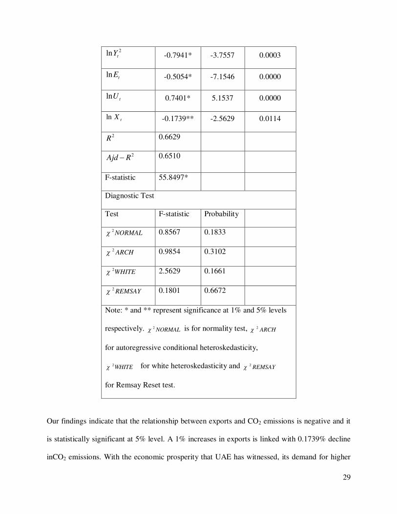
The next step is to examine long run marginal impact of economic growth, electricity
consumption, exports and urbanization on CO2 emissions after fining long run relationship
between them. The results detailed in Table-5 reveal that impact of linear and non-linear terms of
real GDP capita on CO2 emissions is positive and negative at 1 percent level of significance.
This validates the existence of environmental Kuznets curve (EKC) in case of UAE. We find that
a 19.81% increase in CO2 emissions is due to 1% increase in real GDP and negative sign of
squared term seems to corroborate the delinking of CO2 emissions and real GDP at the higher
level of income per capita. This reveals that CO2 emissions increase at the initial stage of
economic growth and decline once economy achieves mature level of per capita income.
Nowadays, the success of a nation takes into account its contribution to the protection of the
environment and natural resources and its efficiency for designing and implementing policies to
improve the living standards of communities without environment degradation. In 2012, UAE
government announced the launch of a long-term national initiative to build green economy in
the UAE entitled “A green economy for sustainable development”. This initiative has three
goals: (i) to make the UAE one of the global pioneers in green economy; (ii) a hub for exporting
and re-exporting green products and technologies, and (iii) a country preserving a sustainable
environment that supports long-term economic growth.
The impact of electricity consumption is negative on CO2 emissions and statistically significant
at 1% level of significant. We find that a 1% increase in electricity consumption declines CO2
emissions by 0.5054%, keeping other things constant. This shows that UAE is using
Page 29
28
environmental friendly source of energy (electricity). The UAE has tried to decrease its
dependency on natural gas and oil for producing electricity. As an alternative, it has encouraged
sustainable development approach, which promotes the use of renewable resources that can
produce pure “clean energy” that can satisfy electricity, cooling and heating demand. The UAE
launched a strategic vision that fosters an investment-friendly ecosystem and innovative planning
in the green economy, implementing a number of programs, projects and initiatives. One of the
most ambitious projects is the creation of a multi-million-dollars solar-energy park managed by
the Dubai Water and Electricity Authority (Dewa). Another example was the establishment of
Masdar city in 2006. The City is accommodated for 40,000 residents, supplied with a fully
integrated eco-friendly energy including solar panels and wind tower. The positive and
statistically significant impact of urbanization on CO2 emissions is found. The rising trend in
urbanization has pressure for housing, public as well as individual transpiration, industrialization,
health facilities raises demand for energy which in resulting; raises CO2 emissions. All else is
same, 0.7401% increase in CO2 emissions is linked with 1% increase in urbanization. As
explained above, massive construction projects to build up approximately from the scratch a
well-developed infrastructure to become a global tourism destination have drastically increased
the air pollution.
Table-5: Long Run Analysis
Dependent Variable = tCln
Variables Coefficient T-Statistic Prob. Values
Constant -36.6285* -4.1980 0.0000
tYln 19.8155* 3.8213 0.0002
Page 30
29
2ln tY -0.7941* -3.7557 0.0003
tEln -0.5054* -7.1546 0.0000
tUln 0.7401* 5.1537 0.0000
tXln -0.1739** -2.5629 0.0114
2R 0.6629
2RAjd 0.6510
F-statistic 55.8497*
Diagnostic Test
Test F-statistic Probability
NORMAL2 0.8567 0.1833
ARCH2 0.9854 0.3102
WHITE2 2.5629 0.1661
REMSAY2 0.1801 0.6672
Note: * and ** represent significance at 1% and 5% levels
respectively. NORMAL2 is for normality test, ARCH
2
for autoregressive conditional heteroskedasticity,
WHITE2 for white heteroskedasticity and REMSAY
2
for Remsay Reset test.
Our findings indicate that the relationship between exports and CO2 emissions is negative and it
is statistically significant at 5% level. A 1% increases in exports is linked with 0.1739% decline
inCO2 emissions. With the economic prosperity that UAE has witnessed, its demand for higher
Page 31
30
environmental quality has increased. Moreover, to become globally competitive, UAE started to
invest massively in the most efficient technologies. Hence, the technique effect has a clear
positive effect on environment quality in case of UAE. Further, Free (industrial) zones in UAE
served by their own ports have reduced considerably the pollutant emissions caused by transport.
We find that there is no evidence of non-normality of error term and same inference is drawn for
autoregressive conditional heteroskedasticity. The results indicate that homoskedasticity exits
and functional form of long run model is well designed confirmed by Ramsey RESET test. This
shows that long run model has passed the assumption of classical linear regression model
(CLRM).
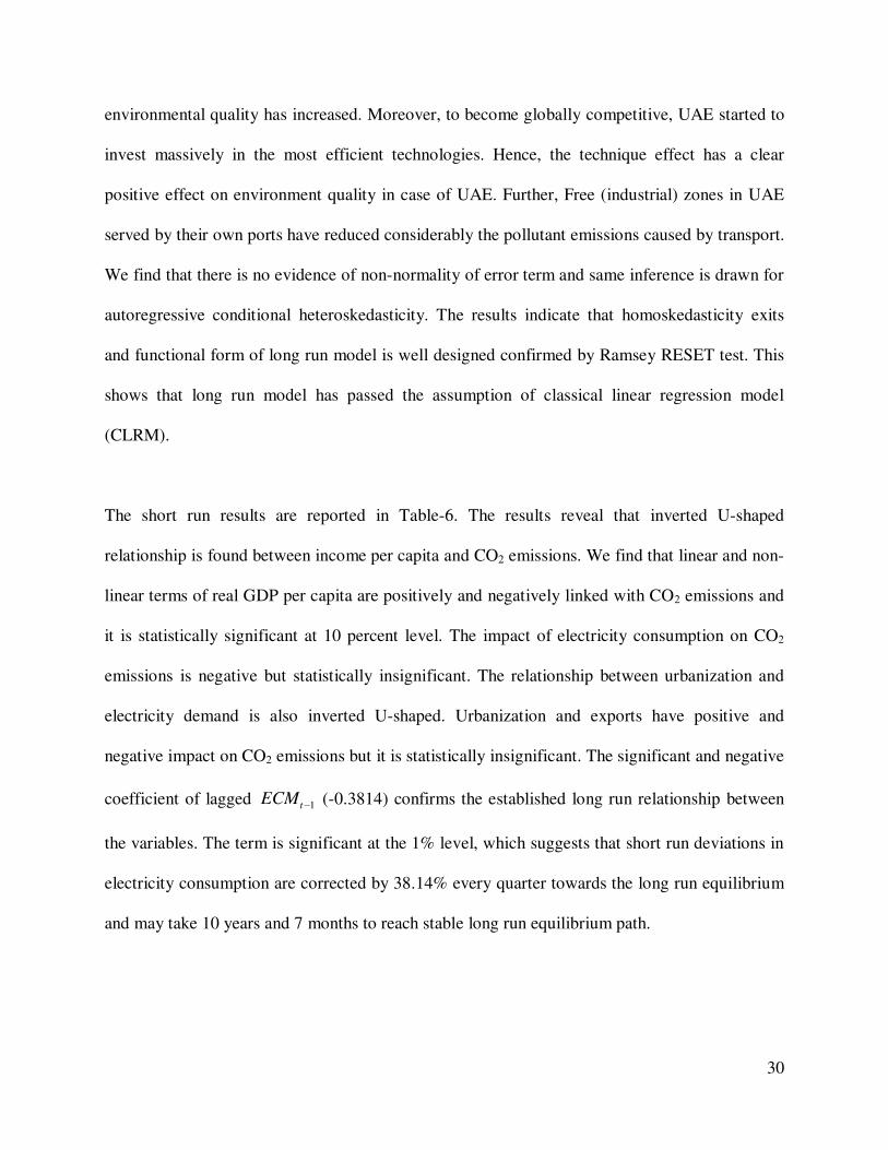
The short run results are reported in Table-6. The results reveal that inverted U-shaped
relationship is found between income per capita and CO2 emissions. We find that linear and non-
linear terms of real GDP per capita are positively and negatively linked with CO2 emissions and
it is statistically significant at 10 percent level. The impact of electricity consumption on CO2
emissions is negative but statistically insignificant. The relationship between urbanization and
electricity demand is also inverted U-shaped. Urbanization and exports have positive and
negative impact on CO2 emissions but it is statistically insignificant. The significant and negative
coefficient of lagged 1tECM (-0.3814) confirms the established long run relationship between
the variables. The term is significant at the 1% level, which suggests that short run deviations in
electricity consumption are corrected by 38.14% every quarter towards the long run equilibrium
and may take 10 years and 7 months to reach stable long run equilibrium path.
Page 32
31
Table-6: Short Run Analysis
Dependent Variable = tCln
Variables Coefficient T-Statistic Prob. Values
Constant -0.0002 -0.1661 0.8683
1ln tC 0.5802* 4.5020 0.0000
tYln 14.4969*** 1.8796 0.0624
2ln tY -0.5820*** -1.8968 0.0600
tCln -0.2012 -0.6196 0.5366
tUln 4.8598 0.8093 0.4198
tXln -0.0102 -0.1075 0.9145
1tECM -0.1152* -2.8729 0.0047
2R 0.3814
2RAjd 0.3486
F-statistic 11.6268*
D.W Test 2.2163
Diagnostic Test
Test F-statistic Probability
NORMAL2 0.6098 0.6102
ARCH2 0.6545 0.4196
WHITE2 0.8083 0.6583
REMSAY2 0.1684 0.6821
Page 33
32
Note: * and*** represent significance at 1% and 10%
levels. NORMAL2 is for normality test, ARCH
2 for
autoregressive conditional heteroskedasticity, WHITE2
for white heteroskedasticity and REMSAY2 for Remsay
Reset test.
The lower segment of Table-6 deals with diagnostic tests. The results indicate that error term has
normal distribution. There is no evidence of autoregressive conditional heteroskedasticity and
same inference is drawn for white heteroskedasticity. The functional form of short run model is
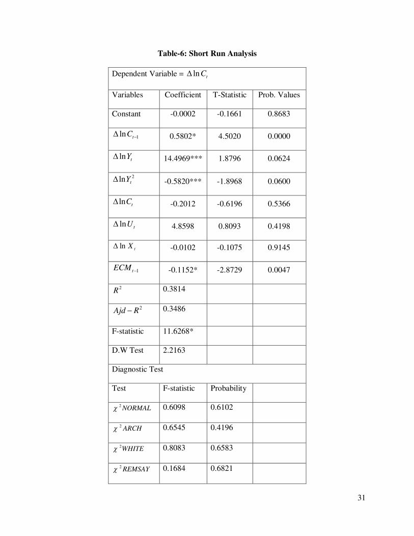
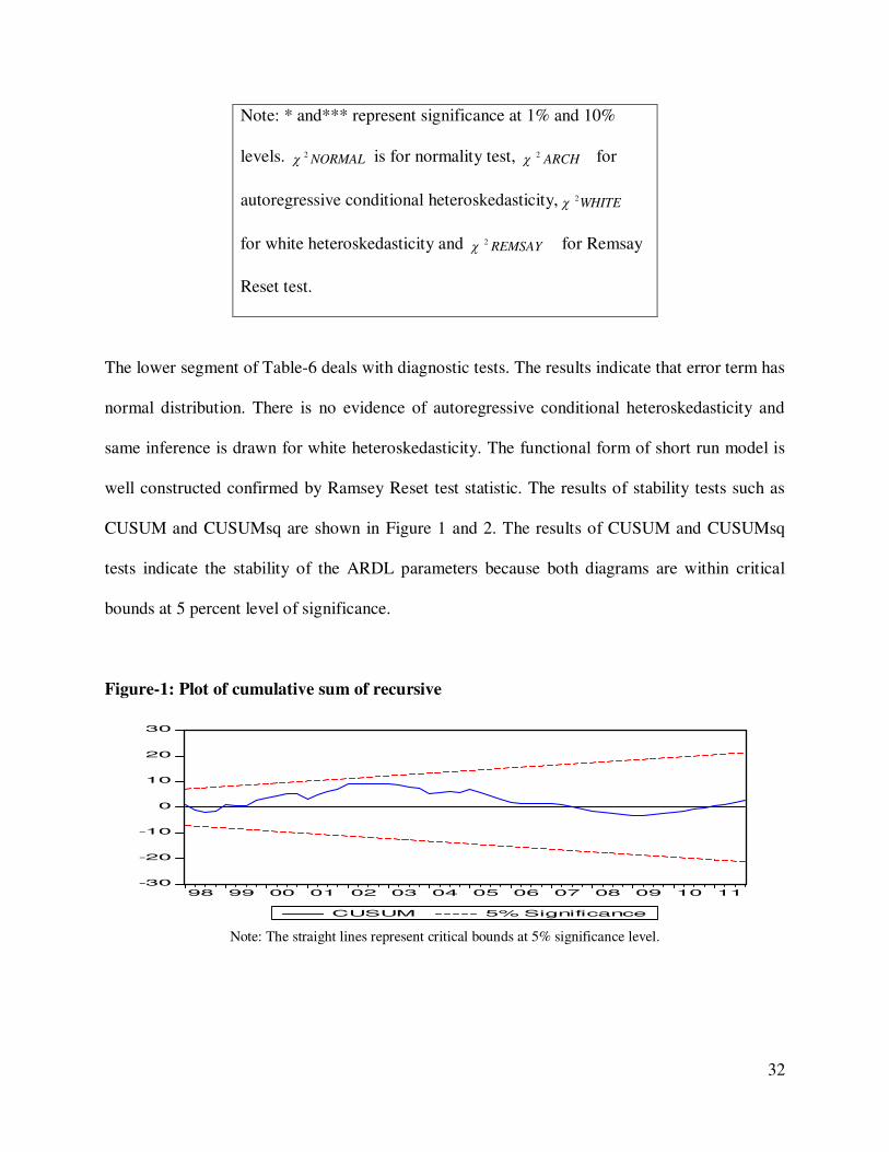
well constructed confirmed by Ramsey Reset test statistic. The results of stability tests such as
CUSUM and CUSUMsq are shown in Figure 1 and 2. The results of CUSUM and CUSUMsq
tests indicate the stability of the ARDL parameters because both diagrams are within critical
bounds at 5 percent level of significance.
Figure-1: Plot of cumulative sum of recursive
Note: The straight lines represent critical bounds at 5% significance level.
-30
-20
-10
0
10
20
30
98 99 00 01 02 03 04 05 06 07 08 09 10 11
CUSUM 5% Significance
Page 34
33
Figure-2: Plot of cumulative sum of squares of recursive residuals
Note: The straight lines represent critical bounds at 5% significance level.
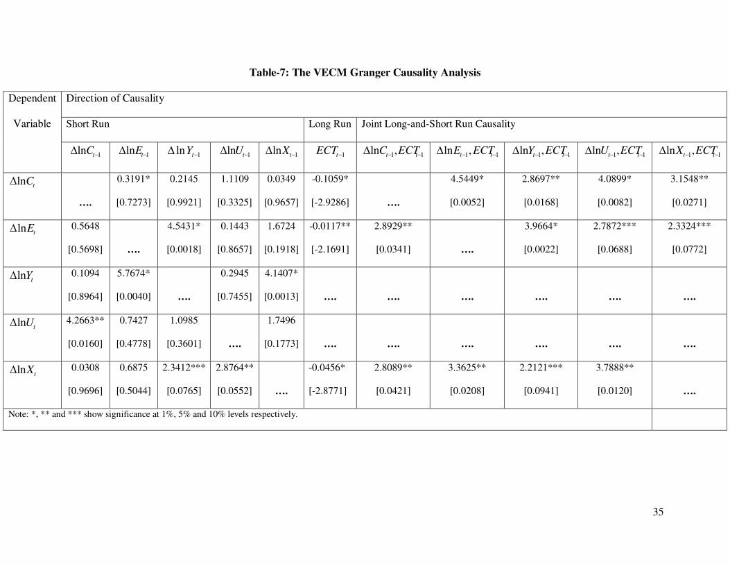
The VECM Granger Causality Analysis
If cointegration is confirmed, there must be uni-or bidirectional causality between/ among the
series. We examine this relation within the VECM framework. Such knowledge is helpful in
crafting appropriate growth, energy and environmental policies for sustainable economic
growth in case of UAE. Table-7 reports results on the direction of long and short run
causality. In long run, we find the bidirectional causality between electricity consumption
and CO2 emissions. This is why the UAE government initiated many projects to produce a
clean energy and reduce CO2 emissions coming from electricity generation from pollutants
process. The causality between exports and electricity consumption supports the existence of
feedback effect. This implies that exports and electricity consumption and exports are
complementary. This implies that exports raise electricity demand and in resulting supply of
electricity enhance more domestic production and hence exports. It suggests in launching of
energy exploration policies for sustainable energy in long run to enhance economic exports
and hence economic growth. Exports and CO2 emissions are Granger cause of each other.
Economic growth Granger causes CO2 emissions validating the existence of the EKC
-0.4
0.0
0.4
0.8
1.2
1.6
01 02 03 04 05 06 07 08 09 10 11
CUSUM of Squares 5% Significance
Page 35
34
hypothesis. This suggests that UAE is growing at the cost of environment that’s why
reduction in CO2 emissions means reduction in economic growth. The UAE government
should adopt energy efficient technology while enhancing domestic production to sustain
long run economic growth and environmental quality. Economic growth Granger causes
electricity consumption and exports. Further, CO2 emissions are Granger cause of
urbanization.
Page 36
35
Table-7: The VECM Granger Causality Analysis
Dependent
Variable
Direction of Causality
Short Run Long Run Joint Long-and-Short Run Causality
1ln tC 1ln tE 1ln tY 1ln tU 1ln tX 1tECT 11,ln tt ECTC 11,ln tt ECTE 11,ln tt ECTY 11,ln tt ECTU 11,ln tt ECTX
tCln
….
0.3191*
[0.7273]
0.2145
[0.9921]
1.1109
[0.3325]
0.0349
[0.9657]
-0.1059*
[-2.9286] ….
4.5449*
[0.0052]
2.8697**
[0.0168]
4.0899*
[0.0082]
3.1548**
[0.0271]
tEln 0.5648
[0.5698] ….
4.5431*
[0.0018]
0.1443
[0.8657]
1.6724
[0.1918]
-0.0117**
[-2.1691]
2.8929**
[0.0341] ….
3.9664*
[0.0022]
2.7872***
[0.0688]
2.3324***
[0.0772]
tYln 0.1094
[0.8964]
5.7674*
[0.0040] ….
0.2945
[0.7455]
4.1407*
[0.0013]
….
….
…. ….
….
….
tUln 4.2663**
[0.0160]
0.7427
[0.4778]
1.0985
[0.3601] ….
1.7496
[0.1773]
….
….
….
…. ….
….
tXln 0.0308
[0.9696]
0.6875
[0.5044]
2.3412***
[0.0765]
2.8764**
[0.0552]
….
-0.0456*
[-2.8771]
2.8089**
[0.0421]
3.3625**
[0.0208]
2.2121***
[0.0941]
3.7888**
[0.0120] ….
Note: *, ** and *** show significance at 1%, 5% and 10% levels respectively.
Page 37
36
In short run, we find unidirectional Granger causality running from electricity consumption
to CO2 emissions. The feedback effect is found between electricity consumption and
economic growth. Exports and economic growth are Granger cause of each other.
Urbanization Granger causes exports and CO2 emissions Granger causes urbanization.
V. Conclusion and Future Research
This study investigates either environmental Kuznets curve (EKC) in case of United Arab
Emirates over the period of 1975Q1-2011Q4. We have applied augmented version of CO2
emissions function by incorporating urbanization and exports. The structural break unit root
test (ZA) is applied to test the integrating properties of the variables. The ARDL bounds
testing is used to examine long run relationship between the variables in the presence of
structural breaks stemming in the series. The causal relationship between is investigated by
applying the VECM Granger causality.
Our empirical evidence presents the support for long run relationship among the variables.
We find that environmental Kuznets curve exists in case of UAE. Electricity consumption
declines CO2 emissions. Urbanization increases CO2 emissions. Exports improve
environmental quality by declining CO2 emissions. The causality results reveal the
bidirectional causality between electricity consumption and CO2 emissions. The feedback
effect is found between electricity consumption and exports and same is true for exports and
CO2 emissions. Economic growth Granger causes CO2 emissions and CO2 emissions is
Granger cause of urbanization.
Page 38
37
Electricity consumption has negative impact on CO2 emissions. This suggests in adopting the
more energy efficient technology which not only produces more clean energy but also lower
CO2 emissions. In this case, adoption of energy conservation policy can be used as tool to
improve the environmental quality to enhance living standards. The feedback effect between
economic growth and CO2 emissions also indicates that UAE is growing at the cost of
environment i.e. rise in economic growth impedes environmental quality. The adoption of
more energy efficient can solve this issue. Urbanization increases CO2 emissions
(Urbanization Granger causes CO2 emissions). This implies that urbanization should be
planned otherwise urbanization impedes environmental. For this purpose, threshold level of
urbanization must be known from where CO2 emissions start to decline i.e. delinking point
between urbanization and CO2 emissions. In future, a study can be conducted to examine the
impact of urbanization on CO2 emissions in case of United Arab Emirates following
Poumanyvong and Kaneko, (2010) because UAE has 84.398% urban population as share of
total population. We can apply unit root test with single and two unknown structural breaks
stemming in the series developed by Narayan and Popp, (2010) and newly development
cointegration approach by Bayer and Hanck, (2012).
Page 39
38
Reference
1. Acquah, H-d., (2010). Comparison of Akaike information criterion (AIC) and Bayesian
information criterion (BIC) in selection of an asymmetric price relationship. Journal of
Development and Agricultural Economics 2, 1-6.
2. Ahmed, K., Long, W., (2012). Environmental Kuznets curve and Pakistan: an empirical
analysis. Procedia Economics and Finance 1, 4-13.
3. Akbostanci, E., Turut-Asık, S., Tunc, I., (2009). The relationship between income and
environment in Turkey: Is there an environmental Kuznets curve? Energy Policy 37, 861–
867.
4. Ang, J. B., (2007). CO2 emissions, energy consumption, and output in France. Energy Policy
35, 4772-4778.
5. Ang, J. B., (2008). Economic development, pollutant emissions and energy consumption in
Malaysia. Journal of Policy Modeling 30, 271-278.
6. Apergis, N., Payne, J. E., (2009). Energy consumption and economic growth: evidence from
the commonwealth of independent states. Energy Economics 31, 641-647.
7. Arouri, M-E., Youssef, A., M’henni, H., Rault, C., (2012). Energy consumption, economic
growth and CO2 emissions in Middle East and North African countries. Energy Policy 45,
342–349.
8. Baek, J., Kim, H-S., (2013). Is economic growth good or bad for the environment? Empirical
evidence from Korea. Energy Economics 36, 744-749.
9. Baum, C. F., (2004). A review of Stata 8.1 and its time series capabilities. International
Journal of Forecasting 20, 151-161.
10. Bayer, C., Hanck, C., (2012). Combining Non-cointegration Tests. Journal of Time Series
Analysis. DOI: 10.1111/j.1467-9892.2012.814.x
11. Chebbi, H. B., (2009). Investigating linkages between economic growth, energy consumption
and pollutant emissions in Tunisia. International Association of Agricultural Economists >
2009 Conference, August 16-22, 2009, Beijing, China.
12. Cole, M. A., Rayner, A.J., Bates, J. M., (1997). The environmental Kuznets curve: An
empirical analysis. Environment and Development Economics 2, 401-416.
Page 40
39
13. Davidsdottir, B., Kaufmann, R. K., Garnham, S., Pauly, P., (1998). The determinants of
atmospheric SO2 concentrations: reconsidering the environmental Kuznets curve. Ecological
Economics 25, 209-220.
14. De Bruyn, S., Van den Bergh, J., Opschoor, J., (1998). Economic growth and emissions:
reconsidering the empirical basis of environmental Kuznets curves. Ecological Economics
25, 161-175.
15. Dickey, D. A., Fuller, W. A., (1979). Distribution of the estimators for autoregressive time
series with a unit root, Journal of the American Statistical Association 74, 427-431.
16. Elliot, G., Rothenberg, T. J., Stock, J. H., (1996). Efficient tests for an autoregressive unit
root. Econometrica 64, 813-836.
17. Esteve, V., Tamarit, C., (2012a). Is there an environmental Kuznets curve for Spain? Fresh
evidence from old data. Economic Modelling 29, 2696–2703
18. Esteve, V., Tamarit, C., (2012b). Threshold cointegration and nonlinear adjustment between
CO2 and income: the environmental Kuznets curve in Spain, 1857–2007. Energy Economics
34, 2148-2156.
19. Fodha, M., Zaghdoud, O., (2010). Economic growth and pollutant emissions in Tunisia: An
empirical analysis of the environmental Kuznets curve. Energy Policy 38, 1150–1156.
20. Fosten, J., Morley, B., Taylor T., (2012). Dynamic misspecification in the environmental
Kuznets curve: Evidence from CO2 and SO2 emissions in the United Kingdom. Ecological
Economics 76, 25–33.
21. Friedl, B., Getzner, M., (2003). Determinants of CO2 emissions in a small open economy.
Ecological Economics 45, 133-148.
22. Grossman, G. M., Krueger, A. B.,(1991). Environmental impacts of a North American Free
Trade Agreement. NBER Working Paper, No. 3914, Washington.
23. Halicioglu, F., (2009). An econometric study of CO2 emissions, energy consumption,
income and foreign trade in Turkey. Energy Policy 36, 1156-1164.
24. He, J., Richard, P., (2010). Environmental Kuznets curve for CO2 in Canada. Ecological
Economics 69, 1083-1093.
25. Hill, R.J., Magnani, E., (2002). An exploration of the conceptual and empirical basis of the
environmental Kuznets curve. Australian Economic Papers 41, 239-254.
Page 41
40
26. Holtz-Eakin, D., Selden, T.M., (1995). Stoking and fires? CO2 emissions and economic
growth. Journal of Public Economics 57, 85-101.
27. Hossain, S., (2012). An econometric analysis for CO2 emissions, energy consumption,
economic growth, foreign trade and urbanization of Japan. Low Carbon Economy 3, 92-105.
28. Hwang, J-H., Yoo, S-H., (2012). Energy consumption, CO2 emissions, and economic
growth: evidence from Indonesia. Quality & Quantity, DOI 10.1007/s11135-012-9749-5.
29. Iwata, H., Okada, K., Samreth, S., (2010). Empirical study on the environmental Kuznets
curve for CO2 in France: The role of nuclear energy. Energy Policy 38, 4057–4063.
30. Jalil, A., Mahmud, S. (2009). Environment Kuznets curve for CO2 emissions: A
cointegration analysis for China. Energy Policy 37, 5167–5172.
31. Jaunky, V-C., (2011).The CO2 emissions-income nexus: Evidence from rich countries.
Energy Policy 39, 1228-1240.
32. Kanjilal, K., Ghosh, S., (2013). Environmental Kuznet’s curve for India: Evidence from tests
for cointegration with unknown structural breaks. Energy Policy, (forthcoming).
33. Kareem, S. D., Kari, F., Alam, G. M., Adewale, A., Oke, O. K., (2012). Energy consumption,
pollutant emissions and economic growth: China experience. The International Journal of
Applied Economics and Finance 6, 136-147.
34. Kuznets, S., (1955). Economic Growth and Income Inequality. The American Economic
Review 45, 1-28.
35. Kwiatkowski, D., Phillips, P., Schmidt, P., Shin, Y., (1992). Testing the null hypothesis of
stationary against the alternative of a unit root: how sure are we that economic time series
have a unit root? Journal of Econometrics 54, 159-178.
36. Lantz, V., Feng, Q., (2006). Assessing income, population, and technology impacts on CO2
emissions in Canada: Where's the EKC? Ecological Economics 57, 229-238.
37. Lindmark, M., (2002). An EKC-pattern in historical perspective: carbon dioxide emissions,
technology, fuel prices and growth in Sweden 1870–1997. Ecological Economics 42, 333-
347.
38. Moomaw, M. R., Unruh, G. C., (1997). Are environmental Kuznets curves misleading us?
The case of CO2 emissions. Environmental and Development Economics 2, 451-63
39. Narayan, P. K., Popp, S., (2010). A new Unit Root Test with two Structural Breaks in Level
and Slope at Unknown Time. Journal of Applied Statistics 37, 1425-1438.
Page 42
41
40. Narayan, P-K., Narayan, S., (2010). Carbon dioxide emissions and economic growth: Panel
data evidence from developing countries. Energy Policy 38, 661-666.
41. Ng, S., Perron, P., 2001. Lag length selection and the construction of unit root test with good
size and power. Econometrica 69, 1519-1554.
42. Ozturk, I., Acaravci, A., (2010). CO2 emissions, energy consumption and economic growth
in Turkey. Renewable and Sustainable Energy Reviews 14, 3220-3225.
43. Panayotou, T., (1997). Dymistifying the Environmental Kuznets curve. Environment and
Development Economics 2, 505-15.
44. Paster, P., (2010). http://www.treehugger.com/clean-technology/ask-pablo-is-indoor-skiing-
really-that-bad.html
45. Pao, H-T, Tsai, C-M., (2010). CO2 emissions, energy consumption and economic growth in
BRIC countries. Energy Policy 38, 7850-7860.
46. Pao, H-T., Yu, H-C., Yang, Y-H., (2011). Modeling the CO2 emissions, energy use, and
economic growth in Russia. Energy 36, 5094-5100.
47. Pesaran, M.H., Shin, Y., Smith, R., (2001). Bounds testing approaches to the analysis of level
relationships. Journal of Applied Econometrics 16, 289-326.
48. Phillips, P. C. B., Perron, P., (1988). Testing for a unit root in time series regression,
Biometrika 75, 335-346.
49. Piaggio, M., Padilla, E., (2012). CO2 emissions and economic activity: Heterogeneity across
countries and non-stationary series. Energy Policy 46, 370-381.
50. Poumanyvong, P., Kaneko, S., (2010). Does urbanization lead to less energy use and lower
CO2 emissions: a cross country analysis. Ecological Economics 70, 434-444.
51. Roberts, J. T., Grimes, P. E., (1997). Carbon intensity and economic development 1962-91: a
brief exploration of the environmental Kuznets curve. World Development 25, 191-198.
52. Roca, J., Padilla, E., Farre, M., Galletto, V., (2001). Economic growth and atmospheric
pollution in Spain: discussing the environmental Kuznets curve hypothesis. Ecological
Economics 39, 85-99.
53. Saboori, B., Sulaiman, J. B., Mohd, M. A., (2011). An empirical analysis of the
environmental Kuznets curve for CO2 emissions in Indonesia: the role of energy
consumption and foreign trade. International Journal of Economics and Finance 4, 243-251.
Page 43
42
54. Saboori, B., Sulaiman, J., Mohd, S., (2012). Economic growth and CO2 emissions in
Malaysia: a cointegration analysis of the Environmental Kuznets Curve. Energy Policy 54,
181-194.
55. Seetanah, B., Vinesh, S., (2010).On the relationship between CO2 emissions and economic
growth: the Mauritian experience. University of Mauritius.
56. Sen, A., (2003). On unit root tests when the alternative is a trend break stationary process.
Journal of Business and Economic Statistics 21, 174-184.
57. Shahbaz, M., Lean, H-H., Shabbir, M-S., (2012). Environmental Kuznets Curve hypothesis
in Pakistan: Cointegration and Granger causality. Renewable and Sustainable Energy
Reviews 16, 2947-2953.
58. Shahbaz, M., Mutascu, M., Azim, P., (2013). Environmental Kuznets curve in Romania and
the role of energy consumption. Renewable and Sustainable Energy Reviews 18, 165–173.
59. Shanthini, R., Perera, K., (2011). Is there a cointegrating relationship between Australia's
fossil-fuel based carbon dioxide emissions per capita and her GDP per capita? International
Journal of Oil, Gas and Coal Technology 7, 182-102.
60. Shuang-Ying, W., Wen-Cong, L., (2011). The relationship between income and NSP in
Zhejiang province: Is there an environmental Kuznets curve? Energy Procedia 5, 1737-1741.
61. Soytasa, U., Sarib, R., Ewing, B., (2007). Energy consumption, income, and carbon
emissions in the United States. Ecological Economics 62, 482-489.
62. Tiwari, A. K., (2011). Primary Energy Consumption, CO2 Emissions and Economic Growth:
Evidence from India. South East European Journal of Economics and Business 6, 99-117.
63. Tiwari, A-K., Shahbaz, M., Hye, Q-M., (2013). The environmental Kuznets curve and the
role of coal consumption in India: Cointegration and causality analysis in an open economy.
Renewable and Sustainable Energy Reviews 18, 519-527.
64. Tucker, M., (1995). Carbon dioxide emissions and global GDP. Ecological Economics 15,
215-223.
65. Zivot, E., Andrews, D., (1992). Further evidence of great crash, the oil price shock and unit
root hypothesis. Journal of Business and Economic Statistics 10, 251-270.