DP 06 050 Titelei - RWI Essenrepec.rwi-essen.de/files/DP_06_050.pdf · The goal of the present...

Rich Iovanna and Colin Vance

No. 50

RWIESSEN

RWI:

Dis

cuss

ion

Pape

rs

Rheinisch-Westfälisches Institutfür WirtschaftsforschungBoard of Directors:Prof. Dr. Christoph M. Schmidt, Ph.D. (President),Prof. Dr. Thomas K. BauerProf. Dr. Wim Kösters

Governing Board:Dr. Eberhard Heinke (Chairman);Dr. Dietmar Kuhnt, Dr. Henning Osthues-Albrecht, Reinhold Schulte

(Vice Chairmen);Prof. Dr.-Ing. Dieter Ameling, Manfred Breuer, Christoph Dänzer-Vanotti,Dr. Hans Georg Fabritius, Prof. Dr. Harald B. Giesel, Dr. Thomas Köster, HeinzKrommen, Tillmann Neinhaus, Dr. Torsten Schmidt, Dr. Gerd Willamowski

Advisory Board:Prof. David Card, Ph.D., Prof. Dr. Clemens Fuest, Prof. Dr. Walter Krämer,Prof. Dr. Michael Lechner, Prof. Dr. Till Requate, Prof. Nina Smith, Ph.D.,Prof. Dr. Harald Uhlig, Prof. Dr. Josef Zweimüller

Honorary Members of RWI EssenHeinrich Frommknecht, Prof. Dr. Paul Klemmer †

RWI : Discussion PapersNo. 50Published by Rheinisch-Westfälisches Institut für Wirtschaftsforschung,Hohenzollernstrasse 1/3, D-45128 Essen, Phone +49 (0) 201/81 49-0All rights reserved. Essen, Germany, 2006Editor: Prof. Dr. Christoph M. Schmidt, Ph.D.ISSN 1612-3565 – ISBN 3-936454-77-9ISBN-13 978-3-936454-77-2

The working papers published in the Series constitute work in progresscirculated to stimulate discussion and critical comments. Views expressedrepresent exclusively the authors’ own opinions and do not necessarilyreflect those of the RWI Essen.

RWI : Discussion PapersNo. 50

Rich Iovanna and Colin Vance

RWIESSEN

Bibliografische Information Der Deutschen BibliothekDie Deutsche Bibliothek verzeichnet diese Publikation in der DeutschenNationalbibliografie; detaillierte bibliografische Daten sind im Internetüber http://dnb.ddb.de abrufbar.

ISSN 1612-3565ISBN 3-936454-77-9ISBN-13 978-3-936454-77-2

Rich Iovanna and Colin Vance*

Satellites and Suburbs: A High-resolution Model ofOpen-space Conversion

AbstractThis study examines the determinants of urbanized area across a 10,000-milesquare swath in central North Carolina, an area undergoing extensive con-version of forest and agricultural land. We model the temporal and spatial di-mensions of these landscape changes using a database that links five satelliteimages spanning 1976–2001 to a suite of socioeconomic, ecological and GIS-created explanatory variables. By specifying the complementary log-log deri-vation of the proportional hazards model, we employ a methodology formodeling a continuous time process – the conversion of land to impervioussurface – using discrete-time satellite data. Spatial effects are captured byseveral variables derived from the imagery that measure the landscape config-uration surrounding a pixel. Empirical results confirm the significance ofseveral determinants of urbanization identified elsewhere in the literature, in-cluding proximity to roads and population density, but also suggest that theparameterization of these variables is biased when the influence of landscapeconfiguration is unaccounted for. We conclude that the inclusion of spatialpattern metrics significantly improves both the explanatory and predictivepower of the estimated model of urbanization.

JEL classification: R14, C41

Keywords: Urbanization, hazard models, satellite imagery

October 2006

*Rich Iovanna, Economic and Planning Analysis Staff, Farm Service Agency, U.S. Department ofAgriculture, Washington DC; Colin Vance, RWI Essen, Germany. – The authors wish to thankManuel Frondel for his comments on an earlier draft. All correspondence to Colin Vance,Rheinisch-Westfälisches Institut für Wirtschaftsforschung (RWI Essen), Hohenzollernstr. 1–3,45128 Essen, Germany, Fax: +49 201 / 81 49-200. Email: [email protected].

1. Introduction

Over the past two decades, the conversion of farm and forestlands on cityfringes throughout the United States has continued unabated, with the ur-banized area expanding from approximately 51 to 76 million acres between1982 and 1997 (Fulton et al. 2001). While partly reflecting growing prosperityand preferences for increased living space, this trend has raised concerns onseveral fronts. Through its strong association to the increase in impervioussurfaces, expansion of the urban frontier eliminates, degrades, and fragmentsnatural habitats, contributes to poor air quality through increased reliance onvehicle travel, and disrupts such ecosystem services as aquifer recharge andnutrient cycling. In turn, such disruptions can impose significant costs on mu-nicipalities, including higher medical costs for air quality-related illnesses andincreased expenditures for the provision of public services and infrastructure.Aesthetic, social, and cultural costs may further compound these ecologicaland health impacts: The movement of populations away from central cityareas has been argued to not only contribute to urban blight (Jargowsky 2001),but also a loss of cultural heritage when farmland and forest is replaced byhelter-skelter development characterized by strip malls, office parks, and dis-connected residential communities (Kunstler 1994).

To the extent that development decisions create landscape mosaics that alterecological function and constrain the choice set of future land-use alternatives,efforts to understand urban expansion can contribute greatly to land-useplanning and environmental policy processes. Such efforts often come in theform of models, and those that are fine scale and spatially explicit are partic-ularly meaningful because of the tight connection between the provision ofhabitat and other services by ecosystems and the pattern of the landscapemosaic in which the ecosystems function. When patches of impervious surfacemanifest in an open-space matrix, the environment is adversely affected asecosystems are fragmented and the ratio of edge to interior area increased.Similarly, where development takes place (e.g., in terms of proximity tosurface waters) may be as relevant as how much when considering impacts(e.g., aquatic ecosystem stress).

In recent years, an increasing number of studies have combined principlesfrom landscape ecology with spatial-econometric methods to describe theeffect of human decision-making, ecosystem function, and their interaction onthe landscape across different spatial scales (e.g., Geoghegan et al. 1997; Klineet al. 2001; Irwin, Bockstael 2002; Fang et al. 2005). Many of these studies havelooked to satellite imagery for their unit of observation, for their dependentvariable, for landscape metrics to explain observed conversion, and to handlestatistical problems emerging from spatial autocorrelation (Turner et al. 1996;Chomitz, Gray 1996; Nelson, Hellerstein 1997; Pfaff 1999; Srinivisan 2005;Vance, Iovanna 2005).

4 Rich Iovanna and Colin Vance

The goal of the present paper is to explore the potential of satellite imagery,and the hazard models derived from it, to explain and predict the conversionof open space to impervious surface. The novelty of our approach relates toboth the degree to which we rely on satellite imagery and the use of amodeling specification well suited to a continuous process that is measured indiscrete time (by the imagery).

The considerable coverage over space and time afforded by satellite imageryis advantageous for projecting trends and for policy simulation. In contrast,simulation can be problematic when datasets are used that do not represent ata fine resolution the entire surface of the region of interest, such as the sampleof fields underlying the National Resources Inventory.

Our observations are the pixels that compose satellite imagery and our de-pendent variable signifies whether or not conversion to impervious surfacehas occurred over the interval of time between two satellite images. We usedata from five images spanning the years 1976–2001 to examine the drivers ofconversion across a 25,900 square kilometer swath in central North Carolina,an area that has lost considerable open space over the last two decades.

Attention in the land-use change literature is turning toward illuminating thestill poorly understood role of natural amenities in the process (Alig et al.2004). Another current theme is how the spatial configuration of land use, byvirtue of its association to both accessibility and spatially determined ame-nities, is, itself, an important determinant of conversion of open space to de-veloped uses. In addition to a broad array of time-varying covariates thatmeasure the land allocation response to the site and locational attributes asso-ciated with each pixel, our model includes GIS-created pattern metrics thatserve as controls for spatial autocorrelation, landscape amenities, and spatialexternalities from neighboring land uses.

Our specification is based on a dynamic, profit-maximizing framework thatsuggests several possible determinants of land conversion from open space toimpervious surface. We subsequently test for the significance of these deter-minants with an empirical model estimating the likelihood of conversion thataccommodates the temporally discrete information on conversion providedby the satellite imagery. While a litany of discrete-choice models already existto examine differences in land cover or use (Lubowski et al. 2003), they areill-suited to policy simulation because they fail to reflect the time dependenceof the conversion process.

Modeling specifications have only recently focused on estimating directly therisk or hazard (instantaneous risk) of conversion.The distinguishing feature ofour model is that it accommodates the temporally discrete information onconversion provided by the satellite imagery. In doing so, the specification

Satellites and Suburbs: A High-resolution Model of Open-space Conversion 5

allows for time-varying covariates, unlike the accelerated failure-time modelin Hite et al. (2003) and estimation of conversion probabilities, unlike Cox re-gression in Irwin et al. (2003).

Our empirical results confirm the hypothesis that pixel-level characteristics –particularly what surrounds a pixel – have a major influence on the likelihoodof its conversion. We also find that the omission of landscape pattern variablescan lead to biased inferences regarding the influence of other covariates, suchas proximity to the urban core, which is commonly identified as an importantdeterminant of land-use change. In addition to parameter and goodness-of-fitestimates, cartographic and nonparametric validation exercises provide addedsupport to an unconstrained model that includes such variables. The paperconcludes with a simple policy simulation that illustrates the model’s practicalmerit.

2. The Study Region

The amount of privately-owned land, the mix of land uses, and the pace ofchange among them were leading considerations for site selection of this ex-ploratory exercise. The study region straddles portions of the Piedmont andthe Inner Coastal Plain of North Carolina, two distinct physiogeographiczones along a north-south axis across the state (Figure 1). Over the centuriesof human occupation, what had been completely forested has been trans-formed into a patchwork that now includes croplands, fields in varying stagesof abandonment, and, increasingly, built-up areas.

The regional economy has transitioned from one based largely on agricultureto one based on the service sector and on manufacturing, with heavy relianceon the forest-products sector. Although the state remains a major producer oftobacco, sweet potatoes, and hog products, the spatial extent of agriculturalproduction has declined drastically since its peak in the early 1900s (Lilly1998). And while the extent of forests has remained relatively stable, peakingin the early 1970s at 20.13 million acres and then dropping back down to ap-proach the 1938 level of 18.1 million acres by 1990 (Brown 1993), the U.S.Forest Service anticipates a loss of 30% of North Carolina’s privately-ownedforest by 2040, with the Interstate 85 corridor extending southward fromRaleigh-Durham designated as a “hotspot” of forest loss due to continuing ur-banization (Prestemon, Abt 2002; Wear, Greis 2002).

In general, North Carolina is is a national leader in terms of land-use change.A highly publicized report recently released from Smart Growth America(Ewing et al. 2003) ranked Greensboro and Raleigh-Durham as second andthird among a listing of 83 U.S. cities in which the spread of development faroutpaces population growth. In Raleigh, for example, the population in-


creased by 32 percent between 1990 and 1996, while its urbanized land area in-creased nearly twofold (Sierra Club 1998).

3. Formalization

Responding to concern about the rate and extent of land-use change requiresunderstanding the causes, timing and location of land-use change. If we knowwhy and when pressures to develop increase for a given tract, we will be in abetter position to evaluate where significant ecological consequences arelikely to occur, as well as the merit of conservation responses. The decision toconvert depends on a complex multiplicity of factors, including the marketvalue of output from the land in alternative uses, expectations about the futureuse of neighboring lands, and the surrounding composition of land ownership.Following the work of Capozza/Helsley (1989) and Boscolo et al. (1998), thetheoretical approach taken here attempts to structure this complexity by as-suming that a unit of land (referred to hereafter as a “pixel” to keep this dis-cussion consistent with the data we ultimately use) will be converted if the netpresent discounted benefits of doing so are greater than the net present dis-counted benefits of leaving the land under its present use. In other words, theland manager converts pixel i in period T to maximize the following objectivefunction:


Figure 1

Source: Adapted from Stear 1973.

The Study Region Boundaries and Physio-geographic Zones of North Carolina

(1) max ( ) ( )T it itt

it itt

TT

t Tt

T

A X D X Cδ δ δ+ −=

∞

=∑∑

0

whereAit : is the return derived from a commodity-based use of the pixel in period t, i.e., the agricul-

tural or forestry rent;Dit is the return to development in period t, i.e., the development rent;X it is a vector of variables that determine returns to development and commodity uses;CT is the cost associated with conversion; andδ is the discount rate, 1/(1+r).

Assuming irreversibility of the conversion process, there are two necessaryconditions for conversion to take place: The first is that the discounted streamof returns derived from conversion are greater than that of leaving the pixel inits present use, net of the one-time conversion costs:

(2) ( ) .D A Cit itt

Tt

− − >=

∞

∑ δ 00

The operative condition, however, is one that will be met well after thatspecified by equation (2): Conversion will occur when the development rentjust equals the opportunity cost, OC, of developing that period as opposed tothe next. Before time T and assuming development rents are rising over timeand conversion costs are declining, it is more profitable to the land owner todefer development for at least another period. After T, the landowner losesmoney every period that development is deferred. More formally, a developedpixel is one in which:

(3) D OC A C Cit it it it it it≥ = + − ++( ) .δ ε1

With equality between development rent in period t and the sum of agri-cultural rent and the cost savings from deferring development, the pixelconverts. Equation (3) indicates that higher development rents hasten con-version, while higher agricultural rents, conversion costs, and the rate ofdecline in costs defer conversion for one pixel relative to another.

The error term inserted in equation (3) accounts for unobserved idiosyncraticfactors associated with pixel i at time t; the greater it is, ceteris paribus, the lesslikely is conversion. If we further specify ε * as the amount that makes (3) anequality, then we find the likelihood of conversion at time t to simply be the cu-mulative density of ε evaluated at ε∗. In other words, if the error for pixel i attime t is less than or equal to ε*, conversion occurs.

In taking the above framework to the empirics, we focus on the critical rolethat timing plays in the risk of conversion. Given that conversion may occur atany point in time during the period under observation and that the factors in-


fluencing conversion are often continuous processes, survival modeling isuniquely suited to the task of estimating the parameters of interest. Ratherthan modeling the direct influence of a covariate on conversion probabilities,survival models are concerned with the hazard rate underlying the proba-bilities, i.e., the instantaneous risk that pixel i is cleared in period t conditionalon not having been converted before t. While conventional methods such aslinear or logistic regression have been applied in these contexts, they areill-equipped to handle the features that often characterize survival data, in-cluding time-varying explanatory variables and censoring or truncation of thedependent variable.

Derived from satellite imagery, our data are interval censored. We knowsimply whether or not an observation’s survival time falls somewhere betweentwo dates. Accordingly, the dependent variable assumes a value of 1 if con-version occurs over an interval between the dates and 0 otherwise. To rec-oncile the temporal continuity of the conversion process being modeled withthis coarseness in the measurement of timing, and because alternative linkfunctions for binary data are inappropriate for such processes, we specify acomplementary log-log survival model. By doing so, the relationship betweenthe X covariates and the probability that opportunity costs (OC) are lowenough for conversion to occur (i.e., that ε is less than or equal to ε*) isassumed to be:

(4) P eOCh= − −1 ,

where

(5) h e X= +α β ... .

It is to the researcher’s considerable advantage to rely on the complementarylog-log link when formulating the generalized linear model for estimationsince it can be derived directly from interval-censored data of event time. As aconsequence, a coefficient estimate’s relationship to the hazard of conversionis unaffected by time, itself. For alternative estimators, such as the logit orprobit, the model fundamentally changes as one shifts consideration from oneinterval to another (Allison 1995).

As a proportional hazards model and a discrete analogue to that developed byCox (1972), the complementary log-log model readily accommodates time-varying covariates and requires no assumptions regarding the functional formof the baseline hazard rate. This enables attention to be focused specifically onthe effect of the covariates on the relative risk of a transition,which is obtainedin a straightforward manner. Unlike the Cox model (such as that used in Irwinet al. 2003), the complementary log-log model is estimated using maximumlikelihood, rather than partial likelihood, allowing one to readily generate es-


timates for the effect of time on the odds of a transition, facilitating themodel’s use for prediction (see Allison 1995, for further discussion).

4. Measurement of Conversion

The econometric model presented in this paper is estimated using a time seriesof five classified Thematic Mapper (TM) and Landsat Multispectral Scanner(MSS) satellite images over central North Carolina for the years 1976, 1980,1986, 1993, 2001. The process of imagery classification was preceded by thestandard pre-processing activities, including geometric correction, spectral-spatial clustering, and radiometric normalization. Classification then pro-ceeded according to a hybrid change detection methodology combining radio-metric and categorical change techniques on a pixel-by-pixel basis. This pro-cedure produced four land cover classes: forest, non-forest vegetation, im-pervious surface, and water. From these classes, we generated a binary de-pendent variable equaling 1 if a conversion from forest or non-forest vege-tation to impervious surface occurred between two dates and 0 otherwise. Ourdata indicate a 67% increase in impervious surfaces between 1976 and 2001,which is roughly consistent with the NRI estimate of a 62% increase in urbanareas for NC as a whole between 1982 and 1997 (USDA 1997b).

Conversions to water were eliminated from the observations used for esti-mation, as were those relating to pixels whose classification in the first year(1976) was either water or impervious surface. Transitions between forest andnon-forest vegetation were also treated as censored as these may be attrib-utable more to forest rotations than permanent conversion from one landcover to another. After overlaying two GIS layers of tenure data from ESRI(2000a, 2000b) and the North Carolina Department of Parks and Recreation(2003), those pixels falling under public ownership (e.g., national, state, andmunicipal parks) were also eliminated.

Upon classifying the imagery, a systematic sample of pixels was drawn thatprovided 65,991 pixels for model estimation. The grid pattern across the sat-ellite scene was such that roughly 1.2 kilometers separated each pixel fromtheir nearest neighbors. Systematic sampling is a commonly applied techniqueto handle spatial correlation of unobserved variables that may emerge fromthe clustering of behavior produced by shared attributes among neighboringunits (Turner et al. 1996; Cropper et al. 2001; Kline et al. 2001). The conse-quences of spatial autocorrelation include inefficient, though asymptoticallyunbiased estimates. However, in cases in which the unobservable variables arespatially correlated with the included explanatory variables, the coefficient es-timates on the included variables will be biased (Irwin, Bockstael 2001). Amajor source of spatial autocorrelation arises from multiple observationsfalling under common landowners (Kline et al. 2001). Given that the average


size of private forest ownership in North Carolina is 9.7 hectares (Powell et al.1992), while the average farm size is approximately 65 hectares (U.S. Census ofAgriculture 1997a), 1.2 kilometer pixel separation was deemed an adequatedistance to minimize the likelihood of drawing pixels for our sample thatbelong to the same owner.

5. Explanatory Variables and Hypothesized Effects

Several static and time-varying covariates are included in the model, thevalues for which correspond to the start year of the interval given by the datesof the satellite imagery (Table 1). The suite of site and locational attributes isintended to reflect the supply and demand side factors that influence the like-lihood of land-use change. In principle, many of these factors could work inboth directions on the conversion hazard, but in what follows we hypothesizethose effects that are likely to dominate.

5.1 Window Metrics

To capture the influence of what Healy (1985) has termed juxtaposition effects– or “spatially bounded externalities that affect adjoining or nearby land”(Alig, Healy 1987: 225) – we derived four time-varying window-based metricsfrom the imagery that measure the landscape configuration surrounding a


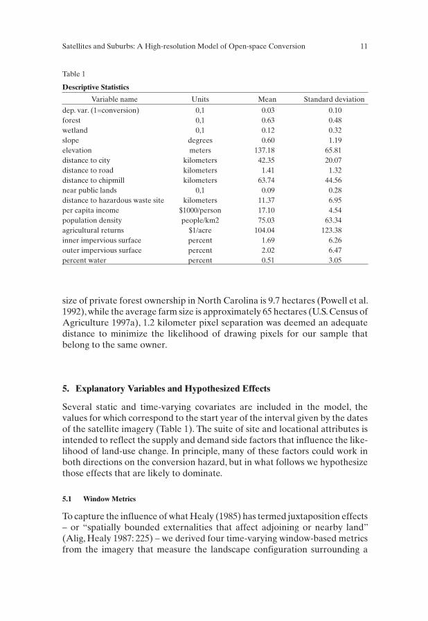
Descriptive Statistics

Variable name Units Mean Standard deviation

dep. var. (1=conversion) 0,1 0.03 0.10forest 0,1 0.63 0.48wetland 0,1 0.12 0.32slope degrees 0.60 1.19elevation meters 137.18 65.81distance to city kilometers 42.35 20.07distance to road kilometers 1.41 1.32distance to chipmill kilometers 63.74 44.56near public lands 0,1 0.09 0.28distance to hazardous waste site kilometers 11.37 6.95per capita income $1000/person 17.10 4.54population density people/km2 75.03 63.34agricultural returns $1/acre 104.04 123.38inner impervious surface percent 1.69 6.26outer impervious surface percent 2.02 6.47percent water percent 0.51 3.05

Table 1

pixel. The first metric is the percent of the area within a window of approxi-mately two square kilometers that is classified as impervious (inner im-pervious surface), which serves as a spatial lag variable to control for the an ad-ditional source of spatial autocorrelation that may emerge from the diffusionof behavior between neighboring units. The window size covers an admittedlyarbitrary area, but one which was based both on best professional judgment ofa typical developer’s spatial frame of reference and on previous studies thathave found window-sizes of similar magnitude to capture spatial externalities(Geoghegan et al. 1997; Fleming, 1999; Irwin, Bockstael 2002). Given the likelypredominance of agglomeration effects associated with impervious surface inthe immediate vicinity of the pixel, we hypothesize the sign of this variable tobe positive.

The second metric complements the first, and is the percent of impervioussurface in a region between the aforementioned window and a larger one withsides twice as large (outer impervious surface). The inclusion of this variable,which is non-overlapping with inner impervious surface, allows for varying pa-rameters with increased distance from the pixel. Such variation may arise, forexample, from spatial externalities associated with neighboring pixels. Whilethe effect of such externalities is expected to vary depending on the sur-rounding configuration of land uses, evidence obtained from Irwin/Bockstael(2002) suggests the net effect to be negative, a finding that they attribute to“repelling effects” associated with low-density residential development. Itbears noting that Irwin/Bockstael use parcel-level data (i.e., each observationbeing a tract of land under common ownership), allowing them to readilyidentify the effects of neighboring land parcels. We acknowledge that theabsence of parcel boundary information here makes it difficult to distinguishtrue externalities associated with a neighboring parcel from spatial effectswithin the parcel itself. With respect to outer impervious surface, however,there are two reasons why any difference between a window-based calculationof imperviousness centered on the parcel and that on an undeveloped pixelwithin the parcel is likely to be negligible. First, the calculation covers a surfacearea that is a kilometer in width and a kilometer removed from the pixel on allsides, so that overlap with the parcel is difficult to conceive. Moreover, to theextent that the undeveloped pixels comprising the sample are within parcelsthat are themselves undeveloped, whatever impervious surface entering incalculation of the metric will be primarily – if not exclusively – associated withneighboring parcels.

The remaining metric, based on the smaller window, is the percent of area clas-sified as water (percent water). The effect of percent water cannot be hypoth-esized a priori: while developers are expected to covet increased water surfacearea as a residential amenity, this feature could also confer benefits to agri-cultural activities.


5.2 Remaining Explanatory Variables

In addition to the window-based metrics, time-varying proximity-basedmetrics are also included in the specification. The first is the Euclideandistance to the nearest woodchip mill (distance to chipmill), which is a poten-tially important cost attribute of forestry operations. Between 1980 and 1998the number of such mills in this region increased from two to 18, a trend thatmany perceive as hastening environmental degradation and biodiversity lossby facilitating the clear-cutting of non-industrial woodlots that is required todevelop the underlying land (Schaberg et al. 2000). Whether the mills therebyincrease the hazard of conversion or alternatively serve to maintain forestedland in a rotation cycle, however, is a question left to the empirical results.

The second proximity metric is the Euclidean distance to the nearest primaryor secondary road (distance to road), which is expected to have a negativeeffect on the conversion hazard given higher access costs. The final proximitymetric (distance to city) measures the Euclidean distance to the nearest citywith a population of over 50,000 (i.e., Charlotte, Durham, Fayetteville,Greensboro, Raleigh, Winston-Salem). As a measure of the influence ofmarket proximity, an increase in this variable is expected to exert a negativeeffect on the conversion hazard. The parameter for fourth proximity metric,the Euclidean distance to the nearest hazardous waste site (distance to haz-ardous waste site), is expected to be positive.

A fifth proximity metric does not change with time and is binary: Near publiclands indicates whether public lands are nearby the pixel (within the outerwindow mentioned, above) and is hypothesized to have a positive coefficientthrough its effect on the amenity value of the pixel.

Additional pixel-level variables are included in the model that do not changewith time, including elevation, slope, and dummy variables indicating forestcover (forest) or wetlands (wetland). All of these variables are expected tohave negative effects given higher conversion costs as well as higher oppor-tunity costs associated with pixels under mature or ecologically important veg-etation.

Varying by county and time interval, a returns to agriculture metric is also inthe model to capture the opportunity costs of commodity uses (agriculturalreturns). This metric, which is expected to negatively affect the conversionhazard, is calculated as county total farm receipts less costs, divided by farmacreage in the county (USDA 1997a). This metric was associated with evenforested pixels, pertaining as it does to the mix of uses to which a farmer mayput their land, including forestry. Two additional time-varying indicators ofcounty-level socioeconomic conditions included in the model are the deflatedper capita income and population density. As proxies for increased demand for


developed land, both variables are expected to increase the conversionhazard.

Finally, we include a set of county dummies representing the counties in theregion that experienced at least one instance of conversion and a set of yeardummies indicating the beginning of each interval. The former serve to limitomitted variable effects arising from county-level differences in governance,zoning, and other factors that may be fixed over time while the latter controlfor the effects of autonomous shifts in the policy and economic environmentthat occur over time in the region as a whole.

6. Results

Table 2 presents results of two complementary log-log models of the deter-minants of the hazard of conversion. The second model (the unconstrainedmodel) is distinguished from the first (the constrained model) by its inclusionof the window-based metrics. Although interpretation of the coefficient es-timates from the complementary log-log model is complicated by the log-oddstransformation of the dependent variable, we can readily calculate their “riskratio”. In the case of the continuous covariates, the risk ratio is interpreted asthe percent change in the hazard rate from a unit increase in the covariate.These values are obtained by subtracting one from eβ and multiplying the re-sulting value by 100. In the case of the dichotomous variables, the risk ratio issimply equal to eβ , and can be interpreted as the ratio of the estimated hazardfor observations with a value of one to the estimated hazard for those with avalue of zero (Allison 1995).

Before discussing the parameter estimates of the two models, we revisit theissue of spatial autocorrelation and whether our sampling approach,combined with the window metrics we include in Model 2, assuages theconcern. Using a modified Moran’s I diagnostic appropriate for limited de-pendent variable models (Kelijian, Prucha 2001), we report some success: At1.05 on the standard normal distribution, we cannot reject the null of nospatial autocorrelation.

While Models 1 and 2 are both highly significant, with chi-square values of2015 and 2460, respectively, a likelihood ratio test of the null-restrictionsimposed by Model 1 on the effects of the window based metrics suggests that itbe rejected in favor of the unconstrained Model 2. The chi-square value of thetest is 445 with four degrees of freedom, providing clear-cut evidence that themetrics improve the fit of the model. In light of our highly unbalanced sample,we refer to Goodman/Kruskal’s gamma (Goodman, Kruskal 1954, 1959, 1963)as an indicator of the predictive performance of the two models. This is anon-parametric, symmetric metric based on the difference between con-


cordant (C) and discordant (D) pairs of predicted and actual values of the de-pendent variable as a percentage of all pairs ignoring ties.Gamma is computedas ( / ) /( )C D C D+ , and can be interpreted as the contribution of the inde-pendent variables in reducing the errors of predicting the rank of the de-pendent variable. The value of gamma calculated from Model 1 is 0.85, while


Complementary log-log Model of the Hazard of Conversion to Impervious Surface

Model 1: Constrained Model Model 2: Unconstrained Model

Coef. est. % Chg. Coef. est. % Chg.

forest –0.682(0.000)

0.506 –0.675(0.000)

0.509

wetland –0.842(0.000)

0.431 –0.694(0.000)

0.500

slope 0.017(0.687)

1.684 0.018(0.687)

1.816

elevation 0.006(0.004)

0.574 0.002(0.380)

0.200

distance to city –0.033(0.000)

–3.227 –0.004(0.494)

–0.399

distance to road –0.941(0.000)

–60.968 –0.536(0.000)

–41.492

distance to chipmill –0.004(0.121)

–0.392 –0.002(0.562)

–0.200

near public lands 0.593(0.000)

1.810 0.185(0.102)

1.203

distance to hazardous waste site –0.175(0.000)

–16.054 –0.084(0.000)

–8.057

per capita income 0.160(0.057)

17.351 0.117(0.169)

12.412

population density 0.012(0.030)

1.157 0.011(0.051)

1.106

agricultural returns –0.003(0.003)

–0.267 –0.003(0.001)

–0.300

Window metricspercent water 0.038

(0.011)3.873

inner impervious surface 0.157(0.000)

17.000

inner impervious surfacesquared

–0.002(0.000)

–0.200

outer impervious surface –0.018(0.010)

–1.784

intercept –5.566(0.000)

–7.502(0.000)

chi2 county dummies (27) 113(0.000)

58(0.000)

chi2 time dummies (3) 149(0.000)

142(0.000)

LR chi2 (60, 46) 2015 2460n_obs 65991 65991

p-values in parenthesis.

Table 2

that of Model 2 is 0.90. The improvement in the predictive ability of the modelwith the inclusion of the window metrics is thus considerable, reducing thefraction of uncertainty remaining in the constrained model by a third.

Turning to the coefficients of the window metrics, all are seen to be highly sig-nificant, with the inner ring variable having the strongest positive effect on theconversion hazard. Its magnitude, however, decreases with increases in im-pervious surface, as evidenced by the negative coefficient of the squared term.Increased water surface also has a positive but somewhat weaker effect, in-creasing the hazard by 3.9%. The only window metric having a negative effectis that measuring the outer band of impervious surface, pointing to thepresence of varying parameters across adjacent bands surrounding the pixel.As noted above, this finding supports research by Irwin/Bockstael (2002), whoemploy similarly constructed variables derived from parcel-level data inMaryland to test for spatial externalities. The negative coefficient in theirs andthe present study suggests that existing development in the vicinity of an unde-veloped pixel reduces the hazard of conversion, a likely reflection of pref-erences for open space. It bears noting that the replication of this result withthe pixel level data used here hinges on the inclusion of the inner impervioussurface metric. Excluding this variable was found – in an unreported model –to result in a positive and significant effect of outer impervious surface, high-lighting the potential for spurious results when spatially lagged effects are un-accounted for.

Beyond improving the fit of the model, the inclusion of the window metricsproduces and resolves several noteworthy discrepancies with respect to thesignificance and magnitude of the remaining covariates. The coefficient on ele-vation is significant but unexpectedly positive in Model 1, a counterintuitiveresult that is resolved by the insignificant estimate in Model 2. Likewise, percapita income and the dummy indicating proximity to public lands, both ofwhich are significant and positive in Model 1, are insignificant at the 5% levelin Model 2. Another discrepancy is seen with respect to the effect of distanceto the nearest city. Model 1 suggests this variable to be a negative and highlysignificant determinant of the conversion hazard, an effect that fades awaywith the inclusion of the window metrics in Model 2. This result likely reflectsa negative bias imparted on the effect of the distance measure in Model 1 re-sulting from the combined influence of the uniformly positive influence ofinner impervious surface on the hazard of conversion together with thenegative correlation between this variable and the variable distance to city(equal to –0.42). More plainly stated, our results may suggest that returns toeconomic activities bear increasingly little relation to the proximity to theurban core, implying, in turn, that a dominant landscape pattern is one charac-terized by sprawl. Taken together, these results suggest that controlling for theinfluence landscape pattern can have a substantial bearing on the conclusions


drawn with respect to other features of the landscape, many of which have im-mediate relevance for policy planning.

The remaining statistically significant variables across the two models arelargely in agreement: Among the stronger effects are the distances to thenearest road and nearest hazardous waste site measures, both of which are sig-nificantly greater than zero for both models. The positive sign on the latter iscounterintuitive at first glance, but may reflect, among other things, the po-tential for larger tracts to be at risk of development in less desirable neigh-borhoods because land is less expensive (Alonso 1964). The variable mea-suring the return to agricultural land uses has the hypothesized negative effecton the hazard of conversion and is of roughly the same magnitude in bothmodels. Likewise, the forest and wetlands dummy both have the expectednegative coefficients. Based on the results from Model 2, forested pixels haveroughly 51% of the hazard of non-forest pixels, with the corresponding mag-nitude for wetlands at 50%.While the coefficients of the 27 county dummies inthe model are not shown in the table, using a chi-square test of their joint sig-nificance we reject the hypothesis at the 1% level that all of these coefficientsare zero in both models. Finally, joint tests of the year dummies are also foundto be statistically significant at the 1% level.

7. Validation

To explore the validity of the models, we developed maps indicating thepattern of development between 1976 and 2001 (i.e., across all four intervals)that is observed and that is predicted by the unconstrained and constrainedmodels. In lieu of selecting an arbitrary threshold probability to identify pre-dicted conversions, we interpolate the predicted probabilities for our sys-tematic sample to create a conversion probability “surface” that spans ourstudy area and is amenable to visual inspection. A “natural neighbor” al-gorithm was employed to generate a raster for this purpose that correspondsto the extent and resolution of our original satellite data (ESRI 2004).

The surface is colored according to the relative magnitude of the estimatedprobability calculated from the parameter estimates of the econometricmodels in Table 2. Dark green indicates where conversion is predicted to beleast likely and red where it’s most likely. The tighter the correspondencebetween the high probability colors and the symbols indicating the 609 ob-served instances of pixel conversion in the sample, the more the estimatedmodel is validated. The performance of the constrained model, seen in Figure2, is not impressive, even without the other one for comparison. The areas ofhigh predicted probability are relatively few and many of the observed con-versions lie outside them. The unconstrained model’s map in Figure 3 depicts agenerally superior picture with crisper transitions between areas of very high


and very low probability. There is also greater correspondence between thehigh probability regions and the instances of actual conversion, including themore dispersed ones.

As a final diagnostic check on the performance of the two models, Figure 4presents their associated receiver-operating characteristic (ROC) curves,which plot the percentage of converted pixels correctly forecast (on the y-axis)against the percentage of non-converted incorrectly forecast (on the x-axis)for each possible prediction threshold. As with the approach used for pro-ducing the maps, a key advantage of constructing ROC curves is that it ob-viates the need to select an arbitrary threshold for designating whether a pre-dicted probability generated by the model correctly predicts a changed pixel.The area under the ROC curve, which ranges from zero to one and isnon-parametric, can be interpreted as the proportion of correct forecastsacross all possible thresholds. The closer the ROC curve is to the diagonal, theless useful is the model for discriminating between open space and convertedpixels. Comparing the two curves, we see that that generated by Model 1 hasan area of 0.91, while the area of the curve generated by Model 2 is slightlyhigher at 0.94. Moreover, a chi-square test that the areas are equal is, at 63.89,clearly rejected, providing further evidence for the superiority of Model 2.


Figure 2

Validation Map for Model 1 (Constrained Model)

8. Simulation

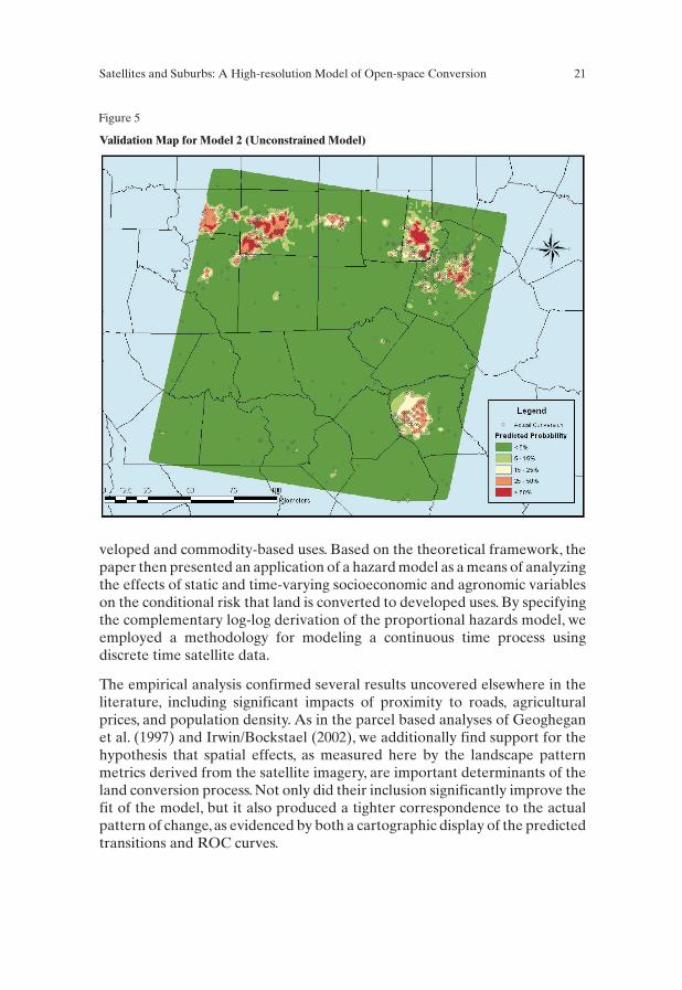
We now illustrate the utility of our modeling approach in terms of policy simu-lation by making a simple comparison between the unconstrained model andits depiction in Figure 2 – the baseline scenario – and a counterfactual scenarioin which all counties are assumed to encourage the conversion process to adegree no greater than that of Durham County (whose effect, ceteris paribus,is relatively low). The simulation approach proceeds interval by interval and isrecursive so that estimated probabilities in a given interval are not only in-fluenced by this modification directly but also via its cumulative effect on thewindow-based metrics.Comparing the resulting map (Figure 5) to the baselineportrayed on Figure 3, we see that applying Durham county’s effect, whichought to reflect in part their particular approach to regional planning, to othercounties results in considerably less conversion over the study area as a whole.

9. Conclusion

This paper began with a theoretical model in which the timing of conversion isdetermined by a comparison of the net discounted returns of the land in de-


Figure 3

Validation Map for Model 1 (Constrained Model)


Figure 4

Receiver operating curves

Model 1

Model 2

veloped and commodity-based uses. Based on the theoretical framework, thepaper then presented an application of a hazard model as a means of analyzingthe effects of static and time-varying socioeconomic and agronomic variableson the conditional risk that land is converted to developed uses. By specifyingthe complementary log-log derivation of the proportional hazards model, weemployed a methodology for modeling a continuous time process usingdiscrete time satellite data.

The empirical analysis confirmed several results uncovered elsewhere in theliterature, including significant impacts of proximity to roads, agriculturalprices, and population density. As in the parcel based analyses of Geogheganet al. (1997) and Irwin/Bockstael (2002), we additionally find support for thehypothesis that spatial effects, as measured here by the landscape patternmetrics derived from the satellite imagery, are important determinants of theland conversion process. Not only did their inclusion significantly improve thefit of the model, but it also produced a tighter correspondence to the actualpattern of change, as evidenced by both a cartographic display of the predictedtransitions and ROC curves.


Figure 5

Validation Map for Model 2 (Unconstrained Model)

These results are significant to a range of issues that have relevance for landuse planning, particularly as regards the siting of roads, protected areas, haz-ardous waste facilities, and other landscape development decisions. Such in-terventions not only leave a direct ecological footprint, but also impact thefuture trajectory of change across adjacent land units. Reliably predicting thelocation, extent, timing and character of these changes is critical to ensuringthat the planning process incorporates the human and environmental di-mensions of the policy options under consideration. The techniques applied inthis study can inform this process by providing both the statistical and spatialconfirmation needed for gauging the impacts that are likely to emerge fromchanges in the variables over which policy makers have leverage.

There are a couple of obvious extensions for using the empirical model es-timated in this paper to explore the issue of urbanization. One useful ex-tension involves acquiring data that make finer distinctions among land-useclasses and allow for a modeling approach that does so as well. A second stagein the form of a multinomial logit, for example, might be applied to thosepixels that convert to examine why they are developed for a particular use(e.g., commercial or low-density residential) as opposed to another.

The simulation exercise we report is merely illustrative, and involved trans-ferring the time invariant factors inherent to one county over to others. Al-though among these factors may be relative differences in approaches tomanaging land-use change, the degree to which this is the case cannot be dis-cerned. Thus, a second extension is to enhance the ability to conduct policysimulations and forecasting. Additional satellite imagery would serve toreduce the interval sizes, rendering the model estimated with these data moreamenable to policy analysis. With information on when and where land usepolicies were promulgated and programs implemented, effects could be as-sessed by adjusting the fixed effects to make room for dummy variables thatare switched on over the relevant dates and across the relevant areas. Evenwithout additional imagery, the model’s flexibility in incorporating the effectsof time on the hazard of conversion could be exploited to facilitate forecasting(Allison 1995). Rather than relying on time dummies, a trend variable mea-suring the time elapsed since some starting date of interest could be includedin the model, such as a change in zoning requirements or the imposition ofsmart growth programs. Such an approach would enable experimentationwith different functional forms of the baseline hazard, including the inclusionof squared and higher order trend terms to allow for nonlinearities in thehazard rate.


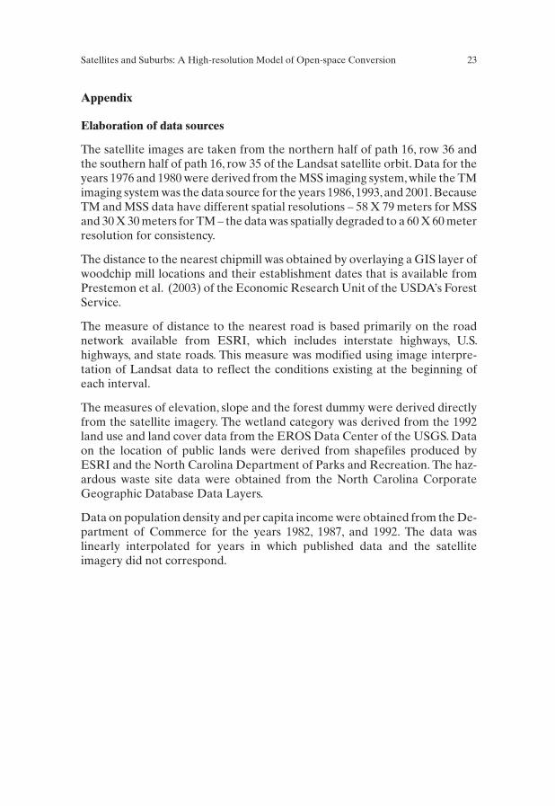
Appendix

Elaboration of data sources

The satellite images are taken from the northern half of path 16, row 36 andthe southern half of path 16, row 35 of the Landsat satellite orbit. Data for theyears 1976 and 1980 were derived from the MSS imaging system, while the TMimaging system was the data source for the years 1986,1993,and 2001.BecauseTM and MSS data have different spatial resolutions – 58 X 79 meters for MSSand 30 X 30 meters for TM – the data was spatially degraded to a 60 X 60 meterresolution for consistency.

The distance to the nearest chipmill was obtained by overlaying a GIS layer ofwoodchip mill locations and their establishment dates that is available fromPrestemon et al. (2003) of the Economic Research Unit of the USDA’s ForestService.

The measure of distance to the nearest road is based primarily on the roadnetwork available from ESRI, which includes interstate highways, U.S.highways, and state roads. This measure was modified using image interpre-tation of Landsat data to reflect the conditions existing at the beginning ofeach interval.

The measures of elevation, slope and the forest dummy were derived directlyfrom the satellite imagery. The wetland category was derived from the 1992land use and land cover data from the EROS Data Center of the USGS. Dataon the location of public lands were derived from shapefiles produced byESRI and the North Carolina Department of Parks and Recreation. The haz-ardous waste site data were obtained from the North Carolina CorporateGeographic Database Data Layers.

Data on population density and per capita income were obtained from the De-partment of Commerce for the years 1982, 1987, and 1992. The data waslinearly interpolated for years in which published data and the satelliteimagery did not correspond.


ReferencesAlig, R., and R. Healy (1987), Urban and Built-Up Area Changes in the United States:

An Empirical Investigation of Determinants. Land Economics 63: 215–226.

Alig, R., J. Kline, and M. Lichtenstein (2004), Urbanization on the US landscape: look-ing ahead in the 21st century. Landscape and Urban Planning 69: 219–234.

Allison, P. D. (1995), Survival Analysis Using the SAS System: A Practical Guide. SASInstitute Inc., Carey.

Alonso, W. (1964), Location and Land Use: Toward a General Theory of Land Rent.Cambridge MA.: Harvard UniversityPress.

Boscolo, M., S. Kerr, A. Pfaff, and A. Sanchez (1998), What Role for Tropical Forests inClimate Change Mitigation? The Case of Costa Rica. Paper prepared for the HIID/INCAE/BCIE Central America Project.

Brown, M.J. (1993), North Carolina’s Forests, 1990. USDA Forest Service TechnicalReport. USFS, Asheville.

Capozza, D.R., and R.W. Helsley (1989), The Fundamentals of Land Price and UrbanGrowth. Journal of Urban Economics 26: 295–306.

Chomitz, K., D. Gray (1996), Roads, land, markets and deforestation: A spatial modelof land use in Belize. World Bank Economic Review 10: 487–512.

Cox, D.R. (1972), Regression Models and Life Tables. Journal of the Royal StatisticalSociety B34: 187–220.

Cropper, M., J. Puri, and C. Griffiths (2001), Predicting the Location of Deforestation.Land Economics 77: 172–186.

ESRI – Environmental Systems Research Institute (2000a), U.S. National Atlas Fed-eral and Indian Land Areas. ESRI Data & Maps 2000 (CD 2).

ESRI – Environmental Systems Research Institute (2000b), U.S. GDT Park Land-marks. ESRI Data & Maps 2000 (CD 3).

ESRI – Environmental Systems Research Institute (2000c), Census 2000 TIGER/ LineData. http://www.esri.com/data/download/census2000_tigerline/, retrieved March2003.

ESRI – Environmental Systems Research Institute (2004), ArcUser July-September2004: 32–35.

Ewing, R., R. Pendall, and D. Chen (2003), Measuring Sprawl and Its Impact.http://www.smartgrowthamerica.com/sprawlindex/MeasuringSprawl.PDF, retrievedFebruary 2003.

Fang,S.,G.Gertner, Z.Sun,and A.Anderson ( 2005),The impact of interactions in spa-tial simulation of the dynamics of urban sprawl. Landscape and Urban Planning 73:294–306.

Fleming, M. (1999), Growth Controls and Fragment Suburban Development: The Ef-fect on Land Values. Geographic Information Sciences 5(2): 154–162.

Fulton, W., R. Pendall, M. Nguyen, and A. Harrison (2001), Who Sprawls Most? HowGrowth Patterns Differ Across the U.S. Center on Urban & Metropolitan Policy.


The Brookings Institution, Washington, DC. http://www.brookings.edu/es/urban/publications/fulton.pdf, retrieved February 2003.

Geoghegan, J., L.A. Wainger, and N.E. Bockstael, N.E. (1997), Spatial landscape indicesin a hedonic framework: an ecological economics analysis using GIS. EcologicalEconomics 23: 251–264.

Goodman, L., and W.H. Kruskal (1954), Measures for association for cross-classifica-tion I. Journal of the American Statistical Association 49: 732–764.

Goodman, L., and W.H. Kruskal (1959), Measures for association for cross-classifica-tion II. Journal of the American Statistical Association 54: 123–163.

Goodman, L., and W.H. Kruskal (1963), Measures for association for cross-classifica-tion III. Journal of the American Statistical Association 58: 310–364.

Healy, R.G. (1985), Population Growth in the U.S. South: Implications for Agriculturaland Forestry Land Supply. Rural Development Perspectives 2: 27–30.

Hite, D., B. Sohngen, and J. Templeton (2003), Zoning, Development Timing, and Agri-cultural Land Use at the Suburban Fringe: A Competing Risks Approach. Agricul-tural and Resource Economics Review, 2003 (April): 145–157.

Irwin, E.G., and N.E. Bockstael (2001), The Problem of Identifying Land UseSpillovers: Measuring the Effects of Open Space on Residential Property Values.American Journal of Agricultural Economics 83: 699–705.

Irwin, E.G., and N.E. Bockstael (2002), Interacting Agents, Spatial Externalities, andthe Endogenous Evolution of Residential Land Use Pattern. Journal of EconomicGeography 2: 31–54.

Irwin, E.G., K.P. Bell, and J. Geoghegan (2003), Modeling and Managing UrbanGrowth at the Rural-Urban Fringe: A Parcel Level Model of Residential Land UseChange. Agricultural and Resource Economics Review 2003 (April): 83–102.

Jargowsky, P.A. (2001), Sprawl, Concentration of Poverty, and Urban Inequality, in: G.Squires, ed., Urban Sprawl: Causes, Consequences & Policy Responses. Washington,DC: Urban Institute Press, http://urbanpolicy.berkeley.edu/pdf/census2000/jargowsky.pdf, retrieved August 2004.

Kelejian, H. H., and I.R. Prucha (2001), On the Asymptotic Distribution of the Moran ITest Statistic withApplications. Journal of Econometrics 104: 219–257.

Kline, J.D., A. Moses, and R.J. Alig (2001), Integrating Urbanization into Landscape-level Ecological Assessments. Ecosystems 4: 3–18.

Kunstler, J.H. (1994), The Geography of Nowhere: The Rise and Decline of America’sMan-Made Landscape. New York: Touchstone Books.

Lilly, J.P. (1998), North Carolina Agricultural History. North Carolina Department ofAgricultural and Consumer Services. http://www.ncagr.com/stats/history/history.htm,retrieved February 2003.

Lubowski, R.N., A.J. Plantinga, and R.N. Stavins (2003), Determinants of Land-UseChange in the UnitedStates 1982–1997. Discussion Paper 03–47. Resources for theFuture, Washington, DC.


Nelson, G., and D. Hellerstein (1997), Do roads cause deforestation? Using satellite im-ages in econometric analysis of land use. American Journal of Agricultural Econom-ics 79: 80–88.

North Carolina Division of Parks & Recreation, Resource Management Program,2003. http://www.ncsparks.net.

North Carolina Corporate Geographic Database Data Layers. http://cgia.cgia.state.nc.us/cgdb/catalog.html

Pfaff, A. (1999), What drives deforestation in the Brazilian Amazon? Evidence fromsatellite and socioeconomic data. Journal of Environmental Economics and Man-agement 37: 26–43.

Powell, D.S., Taulkner, J.L., Darr, D.R., Zhu, Z., MacCleery, D., 1992. Forest Resourcesof the United States. General Technical Report RM–234. USDA Forest Service.

Prestemon, J.P., and R.C. Abt (2002), Timber Products Supply and Demand, in: D.N.Wear and J.G. Greis, eds., The Southern Forest Resource Assessment, USDA ForestService, General Technical Report SRS-53, Asheville, 299–325.

Prestemon, J., J. Pye, D. Butry, and D. Stratton (2000), Economic Research Unit, USDAForest Service. “Locations of Southern Wood Chip Mills for 2000”. http://www.srs.fs.usda.gov/econ/data/mills/chip2000.htm, retrieved April 2003.

Schaberg, R., F.W. Cubbage, and D.D. Richter (2000), Trends in North Carolina TimberProduct Outputs, and the Prevalence of Wood Chip Mills. Paper prepared for thestudy on: Economic and Ecological Impacts Associated with Wood Chip Produc-tion in North Carolina.

Sierra Club, 1998 (1998), Sierra Club Sprawl Report: 30 Most Sprawl-ThreatenedCities. http://www.sierraclub.org/sprawl/report98/raleigh.asp, retrieved January2003.

Srinivasan, S. (2005), Linking land use and transportation in a rapidly urbanizing con-text: A study in Delhi, India. Transportation 32: 87–104.

Stear, T.E. (1973), Population Distribution, in: North Carolina’s Changing Population.University of North Carolina, Carolina Population Center.

Turner, M.G., D.N. Wear, and R.O. Flamm (1996), Land Ownership and Land-CoverChange in the Southern Appalachian Highlands and the Olympic Peninsula. Eco-logical Applications 6: 1150–1172.

USDA – U.S. Department of Agriculture (1997a), Census of Agriculture 1997.

USDA – U.S. Department of Agriculture (1997b), Natural Resources Inventory 1997.

USGS. EROS Data Center (1992), National Land Cover Data 1992. http://edc.usgs.gov/products/landcover/nlcd.html, retrieved January 2003.

Vance, C., and R. Iovanna (2005), Analyzing Spatial Hierarchies in Remotely SensedData: Insights from a Multilevel Model of Tropical Deforestation. Land Use Policy,23: 226–236.

Wear, D.N., and J.G. Greis (2002), The Southern Forest Resource Assessment SummaryReport. USDA Forest Service Southern Research Station. http://www.srs.fs.usda.gov/sustain/report/, retrieved May 2003.


Date post:	17-Sep-2018
Category:	Documents
Upload:	ngodang
View:	213 times
Download:	0 times

DP 06 050 Titelei - RWI Essenrepec.rwi-essen.de/files/DP_06_050.pdf · The goal of the present...

Documents