NASMCR-_/_ • 207793 //_ 3 _"- _'F'

Draft paper for 34 thAIAA/ASME/SAE/ASEE Joint Propulsion Conference, July 13-15,

1998, Cleveland, Ohio

T , /

A GENERALIZED FLUID SYSTEM SIMULATION PROGRAM TO

MODEL FLOW DISTRIBUTION IN FLUID NETWORKS

Alok Majumdar, John W. Bailey, Paul Schallhorn and Todd Steadman

Sverdrup Technology

Huntsville, Alabama - 35806

ABSTRACT

This paper describes a general purpose computer program for analyzing steady state and

transient flow in a complex network. The program is capable of modeling phase changes,

compressibility, mixture thermodynamics and external body forces such as gravity and

centrifugal. The program's preprocessor allows the user to interactively develop a fluid

network simulation consisting of nodes and branches. Mass, energy and specie

conservation equations are solved at the nodes; the momentum conservation equations aresolved in the branches.

The program contains subroutines for computing "real fluid" thermodynamic and

thermophysical properties for 33 fluids. The fluids are: helium, methane, neon, nitrogen,

carbon monoxide, oxygen, argon, carbon dioxide, fluorine, hydrogen, parahydrogen,

water, kerosene (RP-1), isobutane, butane, deuterium, ethane, ethylene, hydrogen sulfide,

krypton, propane, xenon, R-11, R-12, R-22, R-32, R-123, R-124, R-125, R-134A, R-

152A, nitrogen trifluoride and ammonia. The program also provides the options of using

any incompressible fluid with constant density and viscosity or ideal gas.

Seventeen different resistance/source options are provided for modeling momentum

sources or sinks in the branches. These options include: pipe flow, flow through a

restriction, non-circular duct, pipe flow with entrance and/or exit losses, thin sharp

orifice, thick orifice, square edge reduction, square edge expansion, rotating annular duct,

rotating radial duct, labyrinth seal, parallel plates, common fittings and valves, pump

characteristics, pump power, valve with a given loss coefficient, and a Joule-Thompson

device.

The system of equations describing the fluid network is solved by a hybrid numerical

method that is a combination of the Newton-Raphson and successive substitution

methods. This paper also illustrates the application and verification of the code by

comparison with Hardy Cross method for steady state flow and analytical solution for

unsteady flow.

https://ntrs.nasa.gov/search.jsp?R=19980045149 2018-06-15T07:54:59+00:00Z

INTRODUCTION

A fluid flow network consists of a group of flow branches, such as pipes and ducts, that

are joined together at a number of nodes. They can range from simple systems consisting

of a few nodes and branches to very complex networks containing many flow branches

simulating valves, orifices, bends, pumps and turbines. In the analysis of existing or

proposed networks, some node pressures and temperatures are specified or known. The

problem is to determine all unknown nodal pressures, temperatures and branch flow rates.

This program requires that the flow network be resolved into nodes and branches. The

program's preprocessor allows the user to interactively develop a fluid network

simulation consisting of nodes and branches. In each branch, the momentum equation is

solved to obtain the flow rate in that branch. At each node, the conservation of mass,

energy and species equations are solved to obtain the pressures at that node.

The oldest method for systematically solving a problem consisting of steady flow in a

pipe network is the Hardy Cross method [1]. Not only is this method suited for solutions

generated by hand, but it has also been widely employed for use in computer generated

solutions. But as computers allowed much larger networks to be analyzed, it became

apparent that the convergence of the Hardy Cross method might be very slow or even fail

to provide a solution in some cases. The main reason for this numerical difficulty is that

the Hardy Cross method does not solve the system of equations simultaneously. It

considers a portion of the flow network to determine the continuity and momentum

errors. The head loss and the flow rates are corrected and then it proceeds to an adjacent

portion of the circuit. This process is continued until the whole circuit is completed.

This sequence of operations is repeated until the continuity and momentum errors are

minimized. It is evident that the Hardy Cross method belongs in the category of

successive substitution methods and it is likely that it may encounter convergence

difficulties for large circuits. In later years, the Newton-Raphson method has been

utilized [2] to solve large networks, and with improvements in algorithms based on the

Newton-Raphson method, computer storage requirements are not much larger than those

needed by the Hardy Cross method.

The objective of the present effort is to develop: a) a robust and efficient numerical

algorithm to solve a system of equations describing a flow network containing phase

changes, mixing and rotation, and b) to implement the algorithm in a structured, easy-to-

use computer program.

MATHEMATICAL FORMULATION

GFSSP assumes a Newtonian, steady, non-reacting and one dimensional flow in the flow

circuit. The flow can be either laminar or turbulent, incompressible or compressible, with

or without heat transfer, phase change and mixing. The analysis of the flow and pressure

distribution in a complex fluid flow network requires resolution of the system into nodes

and branches. Nodes can be either boundary nodes or internal nodes. Pressures,

temperatures, and concentrations of fluid species are specified at the boundary nodes. At

each internal node, scalar properties such as pressures, temperatures, enthalpies, and

mixture concentrations are computed. The flow rates (vector properties) are computed at

the branches.

GOVERNING EQUATIONS

Figure 1 displays a schematic showing adjacent nodes, their connecting branches, and the

indexing system used by GFSSP. In order to solve for the unknown variables, mass,

energy and fluid specie conservation equations are written for each internal node and flow

rate equations are written for each branch.

[Node I "

lj;? ! .....Single

Fluid

k=l

[Node] Fluid

j=2 ! Mixture

T:mij :,

r

Node:

> i " :

L

/ ' '1

I mji,

Ti

Single N o(:leFluid

l j=4k=2

Fluid

Mixture

' .] Node

mij = - mji

Figure 1 - Schematic of GFSSP Nodes, Branches and Indexing Practice

Mass Conservation Equation

mT+A_ -- m_

AT

j=n

- _ m_

j=l(1)

Equation 1 requires that, for the transient formulation, the net mass flow from a given

node must equate to rate of change of mass in the control volume. In the steady state

formulation, the left hand side of the equation is zero. This implies that the total mass

flow rate into a node is equal to the total mass flow rate out of the node.

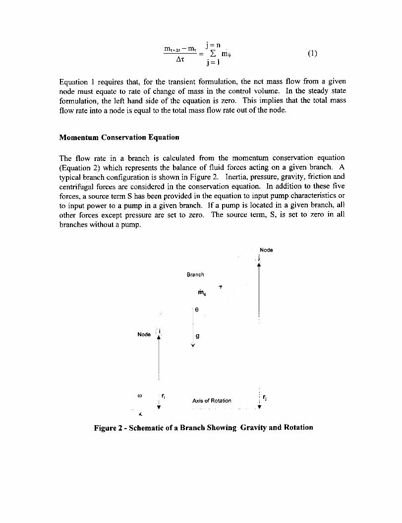
Momentum Conservation Equation

The flow rate in a branch is calculated from the momentum conservation equation

(Equation 2) which represents the balance of fluid forces acting on a given branch. A

typical branch configuration is shown in Figure 2. Inertia, pressure, gravity, friction and

centrifugal forces are considered in the conservation equation. In addition to these five

forces, a source term S has been provided in the equation to input pump characteristics or

to input power to a pump in a given branch. If a pump is located in a given branch, all

other forces except pressure are set to zero. The source term, S, is set to zero in all

branches without a pump.

Node

Branch

mDj

e

g_f

-r

Node

i j :

rl

Axis of Rotation rj

Figure 2 - Schematic of a Branch Showing Gravity and Rotation

m u_+A_- m u_) m0 [ x- Uu /+ --[uij . =

g_ Ax g_

(pi -pj)A+ pgVcos0 Kfmij mij

g¢A+

2 2

p K,.otm A (r_- r_) + S2 g_

(2)

The two terms in the left hand side of the momentum equation represent the inertia of the

fluid. The first one is the time dependent term and must be considered for unsteady

calculations. The second term is significant when there is a large change in area or

density from branch to branch. The first term in the right hand side of the momentum

equation represents the pressure gradient in the branch. The pressures are located at the

upstream and downstream face of a branch. The second term represents the effect of

gravity. The gravity vector makes an angle (0) with the flow direction vector. The third

term represents the frictional effect. Friction was modeled as a product of Kw and the

square of the flow rate and area. Kr is a function of the fluid density in the branch and the

nature of flow passage being modeled by the branch. The calculation of _ for different

types of flow passages has been described in detail later within this report. The fou_h

term in the momentum equation represents the effect of the centrifugal force. This term

will be present only when the branch is rotating as shown in Figure 2. K_ot is the factor

representing the fluid rotation. K_ot is unity when the fluid and the surrounding solid

surface rotates with the same speed. This term also requires a lmowledge of the distances

between the upstream and downstream faces of the branch from the axis of rotation.

Energy Conservation Equation

The energy conservation equation for node i, shown in Figure 1, can be expressed

mathematically as shown in Equation 3.

Ax

; {MAKEmiJ01hiMAXEmj01hi}+MAKImJ01 Kjm:]mi, [(Pi - PJ)+ +Qi

(3)

=0

Equation 3 shows that for transient flow, the rate of increase of internal energy in the

control volume is equal to the rate of energy transport into the control volume minus the

rate of energy transport from the control volume plus the rate of work done on the fluid

by the pressure force plus the rate of work done on the fluid by the viscous force plus therate of heat transfer into the control volume.

For a steady state situation, the energy conservation equation, Equation 3, states that the

net energy flow from a given node must equate to zero. In other words, the total energy

leaving a node is equal to the total energy coming into the node from neighboring nodes

and from any external heat sources (Q3 coming into the node and work done on the fluid

by pressure and viscous forces. The MAX operator used in Equation 3 is known as an

upwind differencing scheme which has been extensively employed in the numerical

solution of Navier-Stokes equations in convective heat transfer and fluid flow applications

[3]. When the flow direction is not known, this operator allows the transport of energy

only from its upstream neighbor. In other words, the upstream neighbor influences its

downstream neighbor but not vice versa. The second term in the right hand side

represents the work done on the fluid by the pressure and viscous force. The difference

between the steady and unsteady formulation lies in the left hand side of the equation.

For a steady state situation, the left hand side of Equation 3 is zero, where as in unsteady

cases the left hand side of the equation must be evaluated.

Fluid Specie Conservation Equation

The flow network shown in Figure 1 has a fluid mixture flowing in most of the branches.

In order to calculate the density of the mixture, the concentration of the individual fluid

species within the branch must be determined. The concentration for the k thspecie can be

written as

+ ' = MAX - mij,0 Cj.k -- MAX n_lij ,0 Ci,k

A'c j_l(4)

For a transient flow, Equation 4, states that the rate of increase of the concentration of

the k th specie in the control volume equals the rate of transport of the k thspecie into the

control volume minus the rate of transport of the k th specie out of the control volume.

Like Equation 3, for steady state conditions, Equation 4 requires that the net mass flow of

the k th specie from a given node must equate to zero. In other words, the total mass flow

rate of the given specie into a node is equal to the total mass flow rate of the same specie

out of that node. For steady state, the left hand side of Equation 4 is zero. For the

unsteady formulation, the resident mass in the control volume is changing and therefore,

the left hand side must be computed.

Thermodynamic and Thermophysical Properties

The momentum conservation equation, Equation 2, requires knowledge of the density and

the viscosity of the fluid within the branch. These properties are functions of the

temperatures, pressures and concentrations of fluid species for a mixture. Three

thermodynamicpropertyroutineshave beenintegratedinto the programto provide therequired fluid property data. GASP [4] provides the thermodynamicand transportpropertiesfor ten fluids. Thesefluids include Hydrogen,Oxygen,Helium, Nitrogen,Methane,CarbonDioxide, CarbonMonoxide, Argon, Neon and Fluorine. WASP [5]providesthethermodynamicandtransportpropertiesfor waterandsteam.GASPAK [6]provides thermodynamic properties for helium, methane, neon, nitrogen, carbonmonoxide,oxygen, argon, carbondioxide, hydrogen,parahydrogen,water, isobutane,butane,deuterium,ethane,ethylene,hydrogensulfide,krypton,propane,xenon,R-I 1, R-12, R-22, R-32, R-123, R-124, R-125, R-134A, R-152A, nitrogen trifluoride andammonia.For RP-1 fuel, a look up tableof propertieshasbeengeneratedby a modifiedversionof GASP. An interpolationroutine hasbeendevelopedto extractthe requiredpropertiesfrom thetabulateddata.

Friction Calculations

It was mentioned earlier in this paper that the friction term in the momentum equation is

expressed as a product of Kf, the square of the flow rate and the flow area. Empirical

information is necessary to estimate Kf. Several options for flow passage resistance are

listed in Table 1.

Table 1 - Resistance Options in GFSSP

Option Type of Resistance

1 Pipe Flow

2 Flow ThroughRestriction

3 Non-circular Duct

4 Pipe with Entrance

and Exit Loss

Input Parameters

L (in), D (in),

e/D

CL, A (in 2)

Option

L (in), D (in),e/D, I%Ko

10

11

Type of Resistance

Rotating RadialDuct

Labyrinth Seal

Input Parameters

L (in), D (in),

N (rpm)

r i (in), c (in), m

(in), n, tx

5 Thin, Sharp Orifice Dt (in), D2 (in) 14 Pump A0, B0, A (in 2)Characteristics'

6 Thick orifice L (in), Dl (in), 15 Pump Power P (hp), r I, A (in 2)

D2 (in)

7 Square Reduction D_ (in), D 2 (in) 16 Valve with Given Cv, A

Cv

8 Square Expansion D I (in), D2 (in) 17 Joule-Thompson Lohm, Vf, k_, ADevice

9 Rotating Annular L (in), ro (in),

Duct r i (in), N (rpm)

Common Fittings

and Valves (Two K

Method)

a (in), b (in) 12 Flow Between ri (in), c (in),

Parallel Plates L (in)

13 D (in), K l, K 2

2

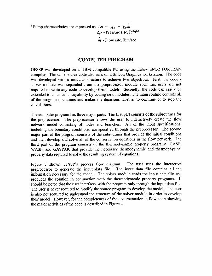
1 Pump characteristics are expressed as Ap = Ao + 13om

Ap - Pressure rise, lbffft 2

m - Flow rate, lbm/sec

COMPUTER PROGRAM

GFSSP was developed on an IBM compatible PC using the Lahey EM32 FORTRAN

compiler. The same source code also runs on a Silicon Graphics workstation. The code

was developed with a modular structure to achieve two objectives. First, the code's

solver module was separated from the preprocessor module such that users are not

required to write any code to develop their models. Secondly, the code can easily be

extended to enhance its capability by adding new modules. The main routine controls all

of the program operations and makes the decisions whether to continue or to stop the

calculations.

The computer program has three major parts. The first part consists of the subroutines for

the preprocessor. The preprocessor allows the user to interactively create the flow

network model consisting of nodes and branches. All of the input specifications,

including the boundary conditions, are specified through the preprocessor. The second

major part of the program consists of the subroutines that provide the initial conditions

and then develop and solve all of the conservation equations in the flow network. The

third part of the program consists of the thermodynamic property programs, GASP,

WASP, and GASPAK that provide the necessary thermodynamic and thermophysical

property data required to solve the resulting system of equations.

Figure 3 shows GFSSP's process flow diagram. The user runs the interactive

preprocessor to generate the input data file. The input data file contains all the

information necessary for the model. The solver module reads the input data file and

produces the solution in conjunction with the thermodynamic property programs. It

should be noted that the user interfaces with the program only through the input data file.

The user is never required to modify the source program to develop the model. The user

is also not required to understand the structure of the solver module in order to develop

their model. However, for the completeness of the documentation, a flow chart showing

the major activities of the code is described in Figure 4.

! !I User !Ii ii

L I '!I

Preprocessor 1IJ

Y

Input

i Data File

,=

Equation Fluid Property

Generator _ _ Programs

EquationSolver

i!

ii

iOutput i

Solver and Propcrq, Module

Figure 3. - GFSSP Process Flow Diagram

/ Start

iV

READ2P0 i InputReads input,

from data _ • file exists

i file. ] Yes ?

PREPROP network,Interactively generate

I_circuit, supply boundary and !

No iinitial conditions.

I _/RITEIN

• Writes data

to a file.

Obt_ntrial 4

solution.

INIT

I_ Generate trial solutionbased on initial guess.

BOUND

Supply time dependant

boundary conditions.

PrintPRINT

probleminput • D. Print headers, boundary and

initial conditions to file.data.

Obtain

solution of NEWTON

pressure & • I,, Controls Newton-Raphsonflowrate solution scheme.

Obtain ENTHALPY

solution of • D. Solution by successive

enthalpy substitution.

No

No

Obtain

solution of •

concentrations

Obtain [,ibranch

resistances

Converged

?

Yes

Print

problem ,Isolution.

MASSC

I_ Solution by successive

substitution.

RESIST 1Calculates resistances •for all branches.

KFACTI - KFACTI7

Calculate branch

resistances.

PRINT

w Print all variables at nodes

and branches to file.

Final

Time Step •ii STOP )? Yes

GASP. WASP and GASPAK

-_ _ Obtain enthalpies for given

pressures and temperatures.

i_ EQNSCalculates residuals

of each equation.l

i

COEF

Calculates coeficients for

correction equations.

sOLVE

• Solve correction equation by

!Gaussian elimination method

UPDATE

m. After applying corrections,

[ update.each variable.

DENSITY 1 GASP, WASP & GASPAK

Calculates density at each node _ • Obtain density of each specie

from law of partial pressure. •from pressure and enthalpy.

Figure 4. GFSSP Flowchart of Major Subroutines

RESULTS & DISCUSSION

The paper also describes comparison of steady state flow network simulation with the

predictions of Hardy Cross method and unsteady flow simulation of tank blow down with

an analytical solution. A typical water distribution network is shown in Figure 5 and

Table 2.

48 psia : 3, 45 psia , 4

A

4T

,946 psia

Figure 5 - Water Distribution Network Schematic

Table 2 - Water Distribution Network Branch Data

Branch Length(inches)

12 120

25 2400

27 2400

57 1440

53 120

56 2400

64 120

68 1440

Diameter(inches) RoughnessFactor

6 0.0018

6 0.0018

5 0.0018

4 0.0018

5 0.0018

4 0.0018

4 0.0018

4 0.0018

78 2400 4 0.0018

89 120 5 0.0018

Figure 6 shows a comparison between GFSSP and Hardy Cross predicted flowrates. The

comparison appears reasonable considering the fact that Hardy Cross method assumes a

constant friction factor in the branch while GFSSP computes the friction factor for each

branch during every iteration. Therefore, as the flowrates change the friction factor also

changes.

1.6

1.2I

0.8

^_ 0.6 I_ 0.2

-0.2

-0.4

IQ-GFSSP Solution (ff^3/sec)

rlQ - Hardy Cross Prediction (fl^3/sec)

Figure

12 25 27 53 56 57 64 68 78 89

Branch Number

6. - A Flow Rate Comparison Between GFSSP and Hardy Cross Method

Predictions

Blowdown of a Tank

Figure 7 shows a tank with an internal volume of 10 ft 3 containing nitrogen gas at a

pressure and temperature of 100 psia and 80 °F respectively. The nitrogen is discharged

into the atmosphere through an orifice with a 0.1 inch diameter until the pressure in the

tank becomes 50 psia.

Tank

v= 10fP

Initial Condition

Pl = 100 psia

T i = 80OF

d=0.1 in

Atmospherep = 14.7 psia

(a) (b)

Figure 7. - Physical Schematic (a) and GFSSP Model (b) for Venting Nitrogen Tank

Analytical Solution:

The differential equation governing an isentropic blow down process can be written as:

(___,/('-3_'j2' d(p/ ) TA x/,rgcp, p,(_____l (5)

p Pi 2 <r+_)/2(r-_)

dx p,V

This is an initial value problem and the initial conditions are:

x=0, P=l

Pi

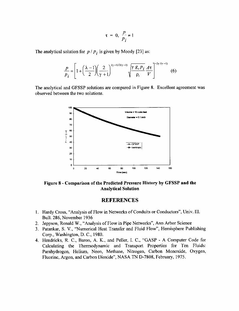
The analytical solution for p / Pi is given by Moody [23] as:

Pip -[1+ (--_-)(_--]-)k-12 <y+l)/2_y-l)/'_

gcPi Ax

Pi V

The analytical and GFSSP solutions are compared in Figure 8.observed between the two solutions.

-2"¢/(_:-l)

(6)

Excellent agreement was

90 =

8O

70

5O

40

3O

20

10

0 i I i i i

20 40 60 80 100 120 140

Time (=ec}

160

Figure 8 - Comparison of the Predicted Pressure History by GFSSP and the

Analytical Solution

REFERENCES

1. Hardy Cross, "Analysis of Flow in Networks of Conduits or Conductors", Univ. Ill.

Bull. 286, November 1936

2. Jeppson, Ronald W., "Analysis of Flow in Pipe Networks", Ann Arbor Science

3. Patankar, S. V., "Numerical Heat Transfer and Fluid Flow", Hemisphere Publishing

Corp., Washington, D. C., 1980.

4. Hendricks, R. C., Baron, A. K., and Peller, I. C., "GASP - A Computer Code for

Calculating the Thermodynamic and Transport Properties for Ten Fluids:

Parahydrogen, Helium, Neon, Methane, Nitrogen, Carbon Monoxide, Oxygen,

Fluorine, Argon, and Carbon Dioxide", NASA TN D-7808, February, 1975.

5. Hendricks,R. C., Peller, I. C., and Baron,A. K., "WASP - A Flexible FortranIVComputerCodefor CalculatingWater and SteamProperties",NASA TN D-7391,November,1973.

6. CryodataInc., "User'sGuideto GASPAK,Version3.20",November,1994.1. 7.Moody, F. J., "Introduction to UnsteadyThermofluid Mechanics",John Wiley,

1990.