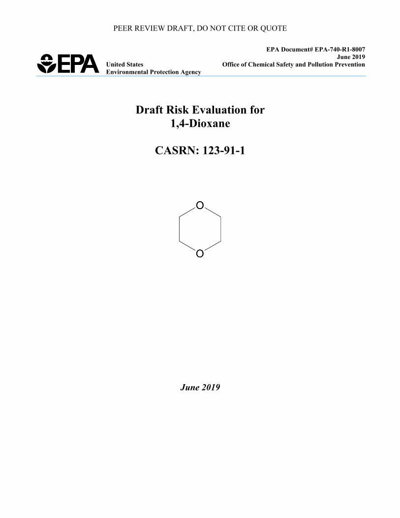
PEER REVIEW DRAFT, DO NOT CITE OR QUOTE EPA Document# EPA-740-R1-8007 June 2019 United States Office of Chemical Safety and Pollution Prevention Environmental Protection Agency Draft Risk Evaluation for 1,4-Dioxane CASRN: 123-91-1 June 2019
Transcript
PEER REVIEW DRAFT, DO NOT CITE OR QUOTE
EPA Document# EPA-740-R1-8007 June 2019
United States Office of Chemical Safety and Pollution Prevention Environmental Protection Agency
Draft Risk Evaluation for 1,4-Dioxane
CASRN: 123-91-1
June 2019
PEER REVIEW DRAFT, DO NOT CITE OR QUOTE
2 of 407
TABLE OF CONTENTS 1 EXECUTIVE SUMMARY ..............................................................................................................18
2.1 Physical and Chemical Properties ...............................................................................................24 2.2 Uses and Production Volume ......................................................................................................25 2.3 Regulatory and Assessment History ...........................................................................................26 2.4 Scope of the Evaluation ...............................................................................................................28
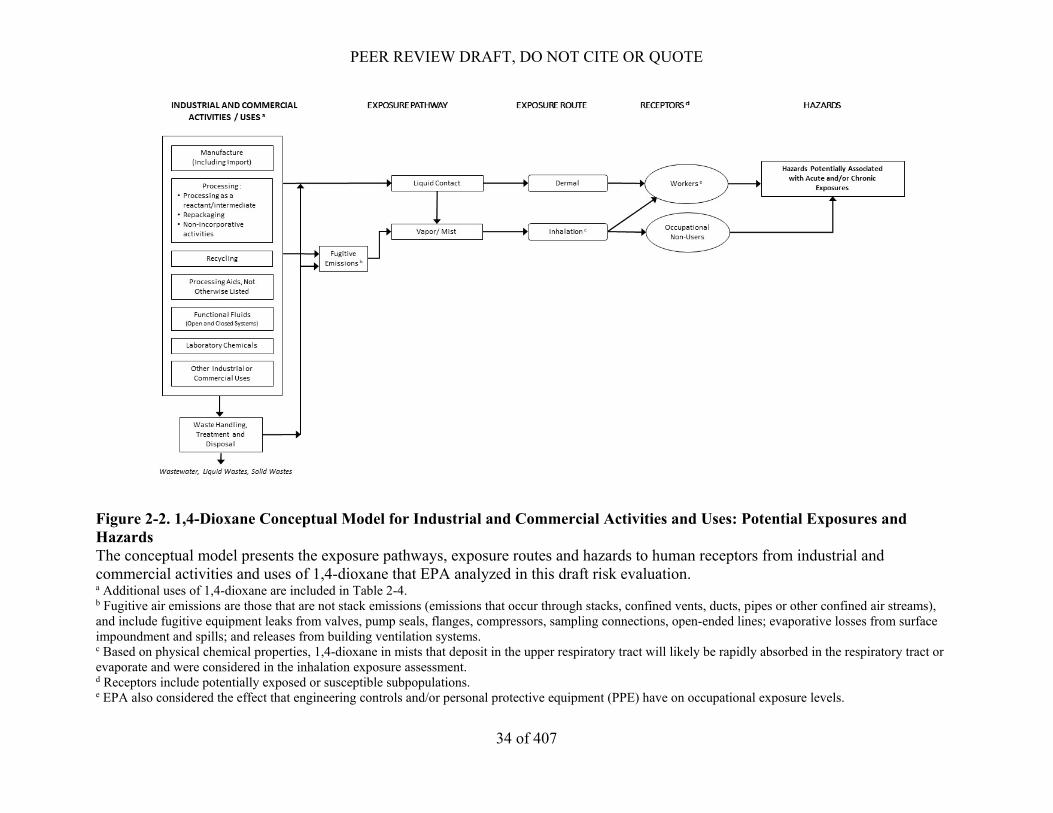
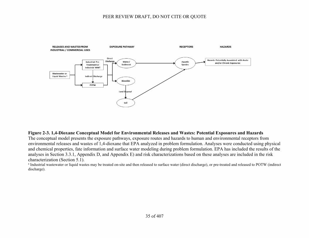
Conditions of Use Included in the Risk Evaluation ............................................................... 28 Conceptual Models ................................................................................................................ 32
2.5 Systematic Review ......................................................................................................................36 Data and Information Collection ........................................................................................... 36 Data Evaluation ..................................................................................................................... 42 Data Integration ..................................................................................................................... 42
4.1 Ecological Hazards ......................................................................................................................79 Approach and Methodology .................................................................................................. 79 Hazard Identification- Toxicity to Aquatic Organisms ......................................................... 80
4.2 Human Health Hazards ...............................................................................................................80 Approach and Methodology .................................................................................................. 80 Toxicokinetics ........................................................................................................................ 82 Hazard Identification ............................................................................................................. 85
4.2.3.1 Non-Cancer Hazards ...................................................................................................... 85 4.2.3.2 Genetic Toxicity and Cancer Hazards ............................................................................ 92
PEER REVIEW DRAFT, DO NOT CITE OR QUOTE
3 of 407
Potential Modes of Action for 1,4-Dioxane Toxicity ............................................................ 98 Evidence Integration and Evaluation of Human Health Hazards ........................................ 105 Dose-Response Assessment ................................................................................................. 108
4.2.6.1 Potentially Exposed or Susceptible Subpopulations .................................................... 108 4.2.6.2 Points of Departure for Human Health Hazard Endpoints ........................................... 108
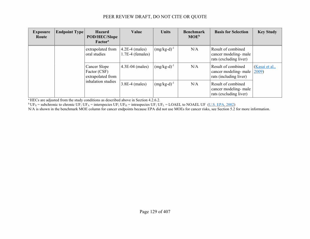
4.2.6.2.1 Acute/Short-term POD for Inhalation Exposures ................................................. 109 4.2.6.2.2 Acute/Short-term POD for Dermal Exposures extrapolated from Inhalation Studies ................................................................................................................... 110 4.2.6.2.3 Chronic Non-Cancer POD for Inhalation Exposures ............................................ 111 4.2.6.2.4 Chronic Cancer Unit Risk for Inhalation Exposures i.e. Inhalation Unit Risk (IUR)– ............................................................................................................................. 115 4.2.6.2.5 Chronic Non-Cancer POD for Dermal Exposures extrapolated from Chronic Inhalation Studies ................................................................................................................... 117 4.2.6.2.6 Chronic Non-Cancer POD for Dermal Exposures extrapolated from Chronic Oral Studies ............................................................................................................................. 119 4.2.6.2.7 Chronic Cancer Unit Risk for Dermal Exposures i.e. Cancer Slope Factor (CSF) extrapolated from Chronic Inhalation Studies ........................................................................ 122 4.2.6.2.8 Chronic Cancer Unit Risk for Dermal Exposures i.e. Cancer Slope Factor (CSF) extrapolated from Chronic Oral Studies ................................................................................. 123 Summary of Human Health Hazards ................................................................................... 128
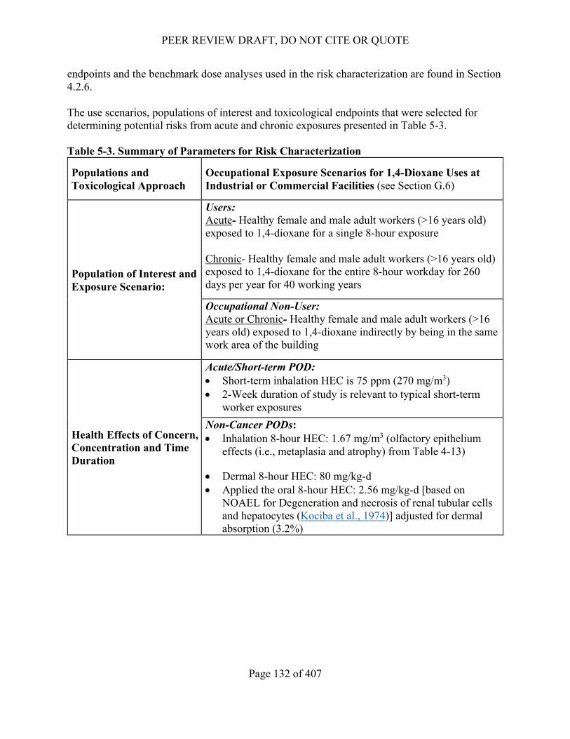
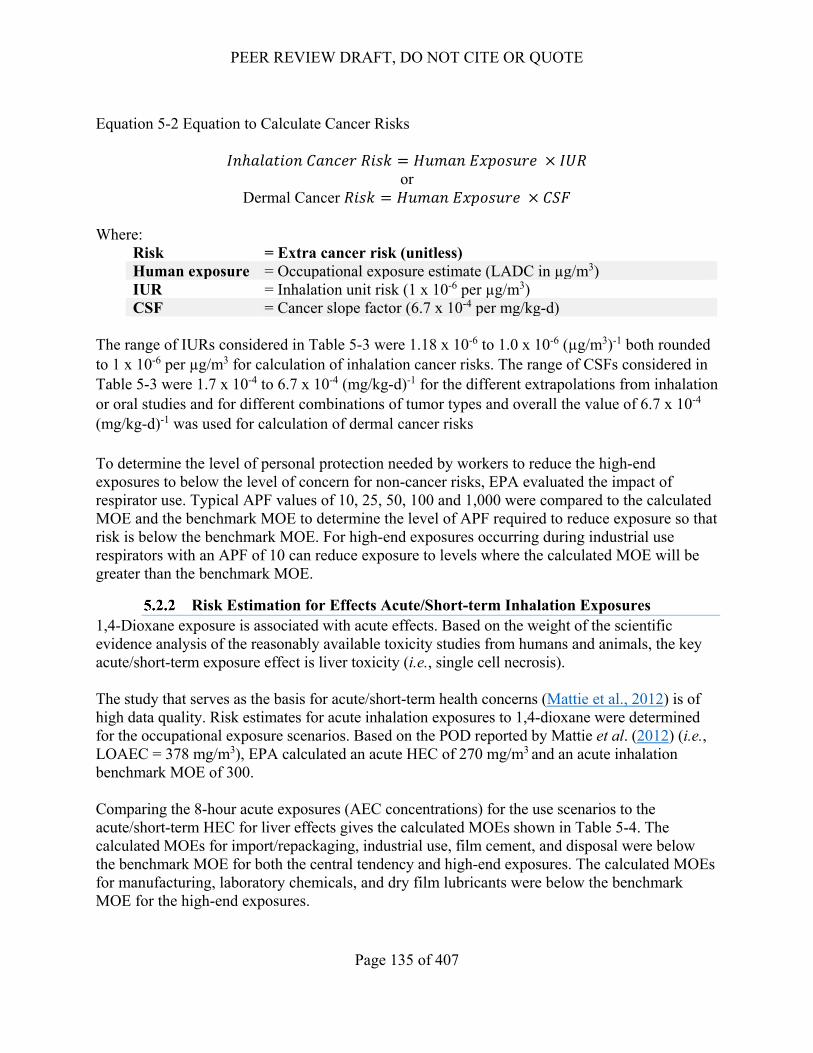
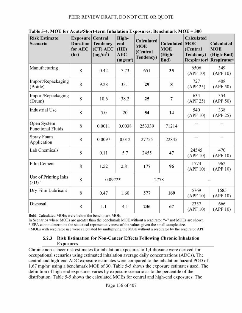
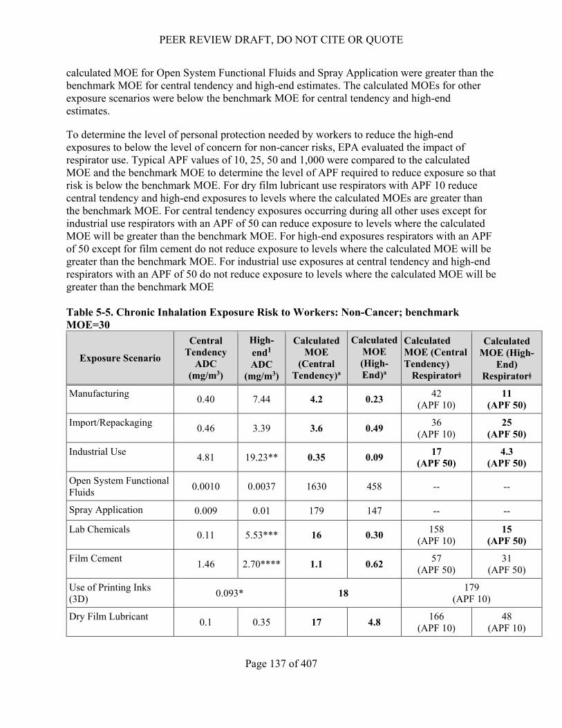
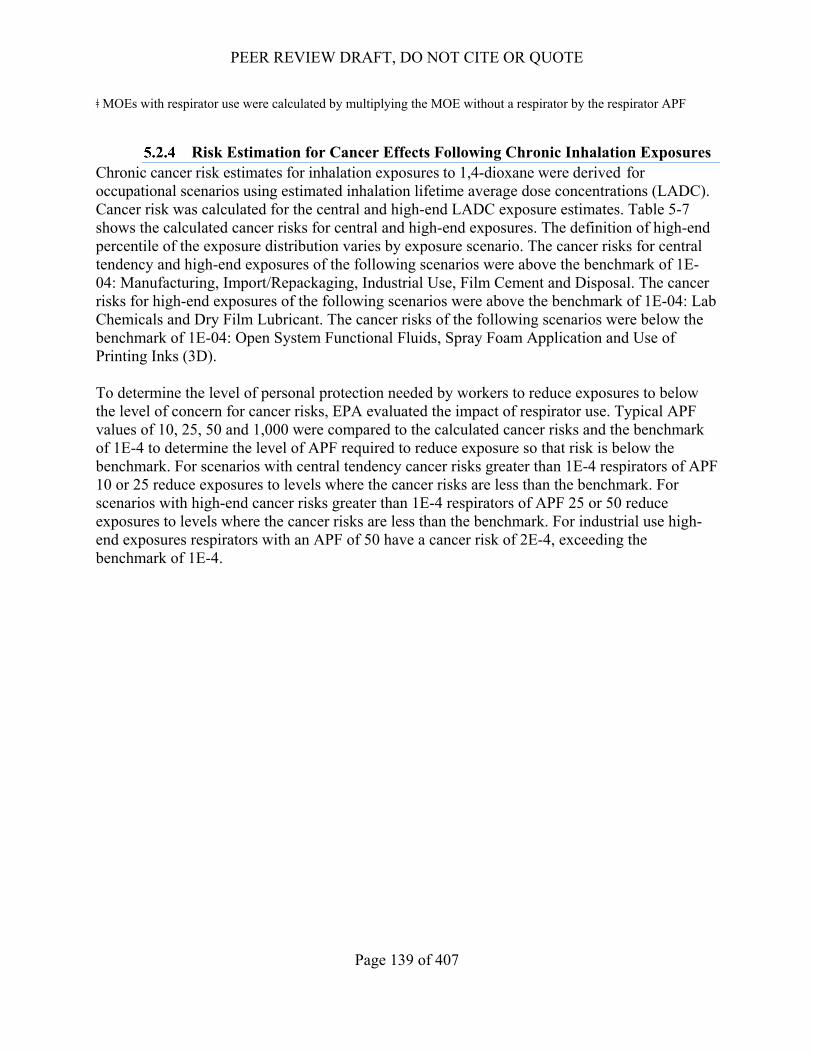
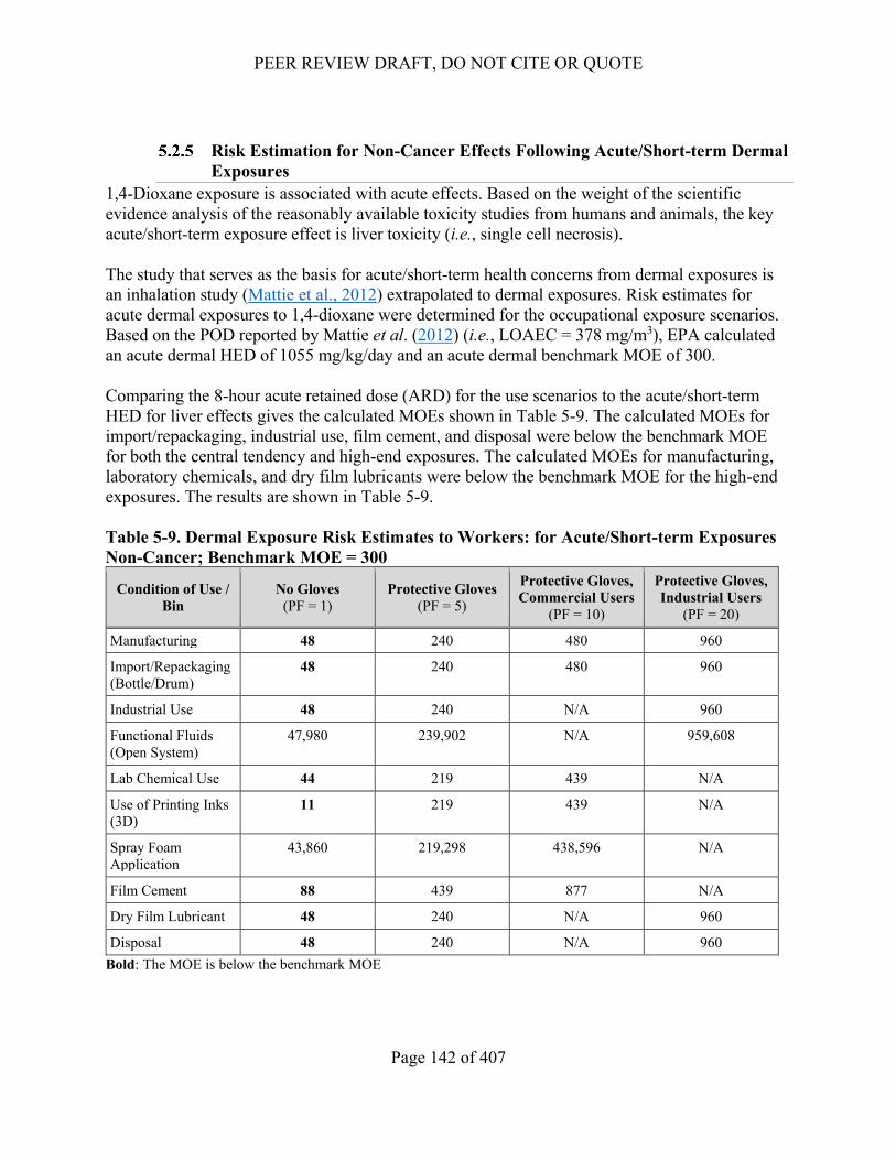
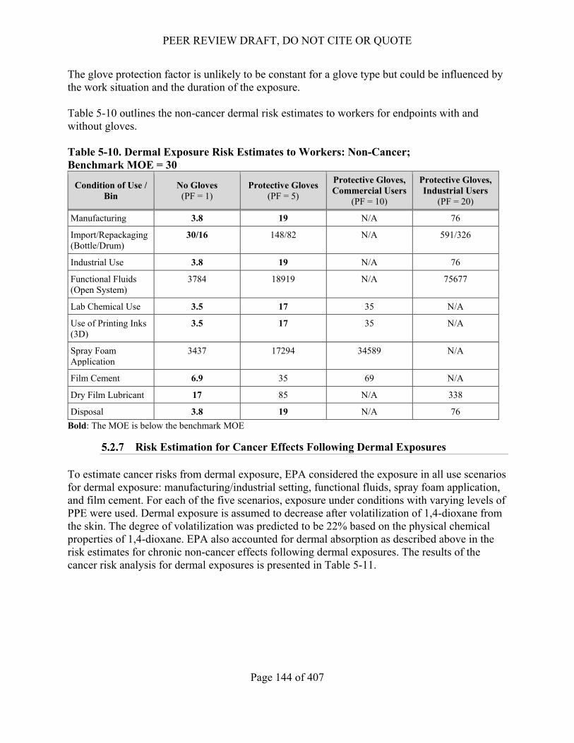
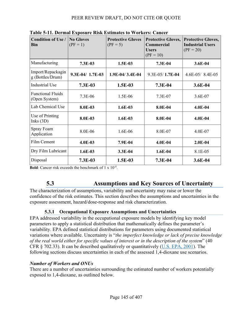
5.2 Human Health Risk ...................................................................................................................131 Human Health Risk Estimation Approach .......................................................................... 131 Risk Estimation for Effects Acute/Short-term Inhalation Exposures .................................. 135 Risk Estimation for Non-Cancer Effects Following Chronic Inhalation Exposures ........... 136 Risk Estimation for Cancer Effects Following Chronic Inhalation Exposures ................... 139 Risk Estimation for Non-Cancer Effects Following Acute/Short-term Dermal Exposures 142 Risk Estimation for Non-Cancer Effects Following Chronic Dermal Exposures ............... 143 Risk Estimation for Cancer Effects Following Dermal Exposures ..................................... 144
5.3 Assumptions and Key Sources of Uncertainty ..........................................................................145 Occupational Exposure Assumptions and Uncertainties ..................................................... 145 Environmental Hazard and Exposure Assumptions and Uncertainties ............................... 148 Human Health Hazard Assumptions and Uncertainties ...................................................... 148 Risk Characterization Assumptions and Uncertainties ........................................................ 150
5.4 Potentially Exposed or Susceptible Subpopulations……………………………………………152 5.5 Aggregate and Sentinel Exposures……………………………………………………………..153 6 RISK DETERMINATION ............................................................................................................151
6.1 Unreasonable Risk.....................................................................................................................152 Overview .............................................................................................................................. 152 Risks to Human Health ........................................................................................................ 154
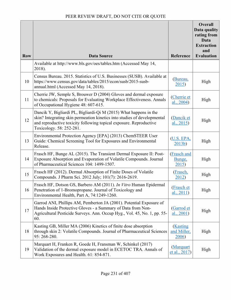
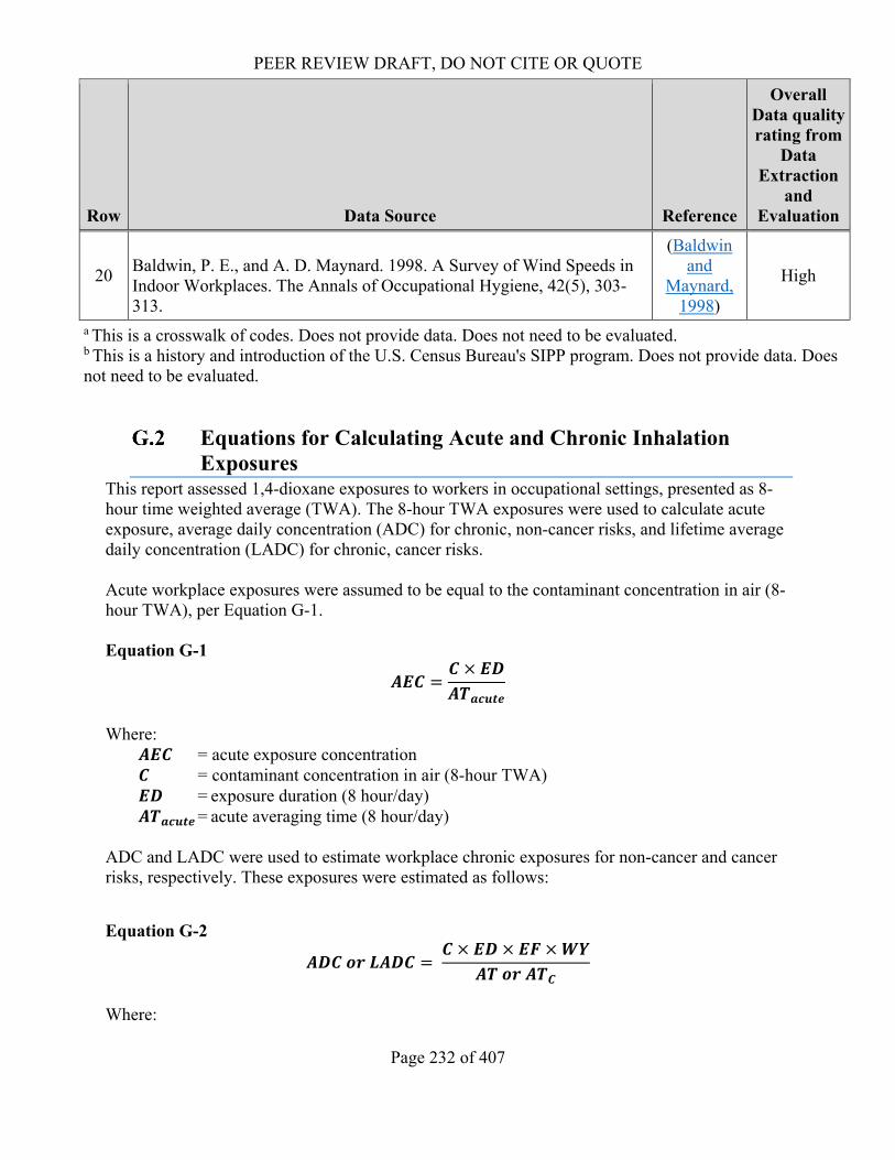
G.1.1 Evaluation of Inhalation Data Sources Specific to 1,4-Dioxane ..........................................224 G.1.2 Evaluation of Cross-Cutting Data Sources ...........................................................................230
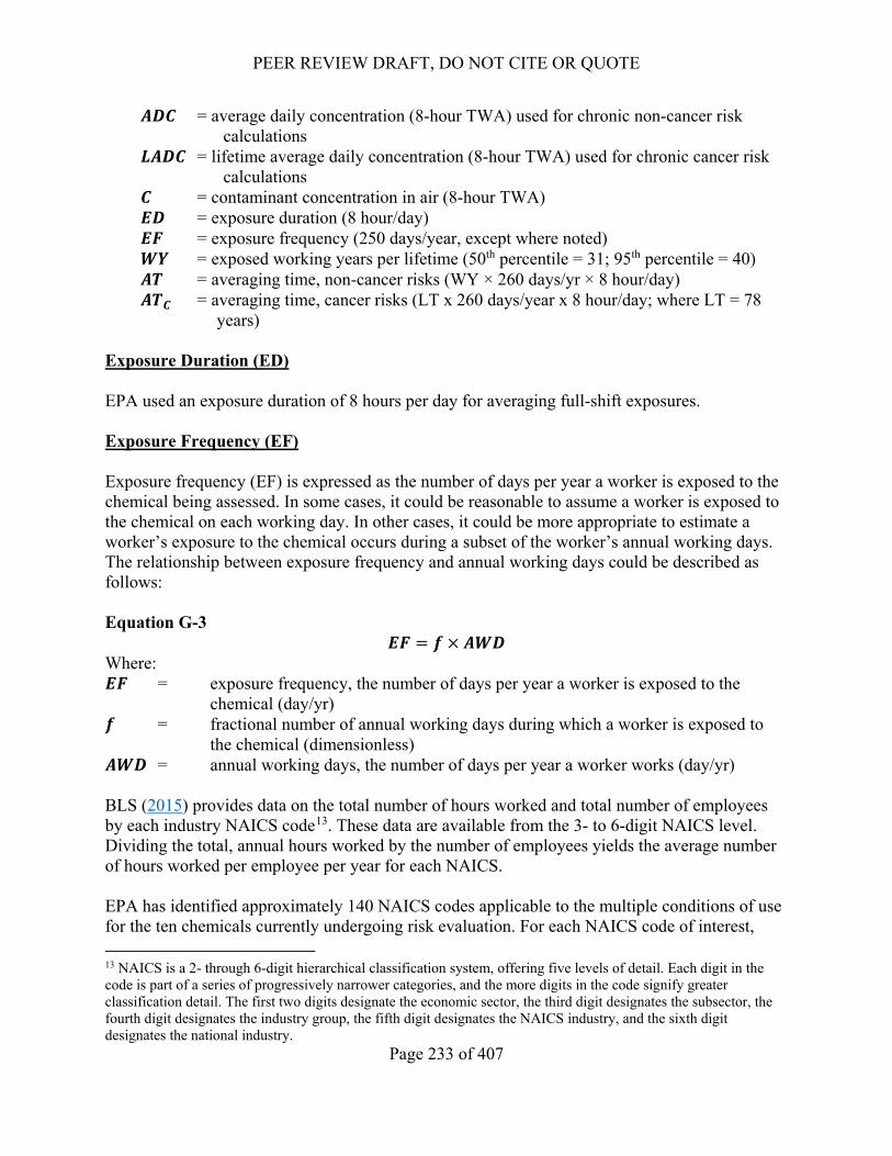
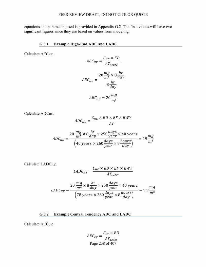
G.3.1 Example High-End ADC and LADC ...................................................................................238 G.3.2 Example Central Tendency ADC and LADC ......................................................................238
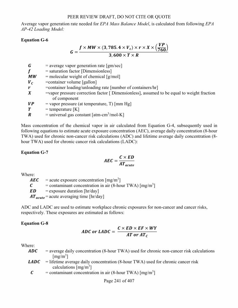
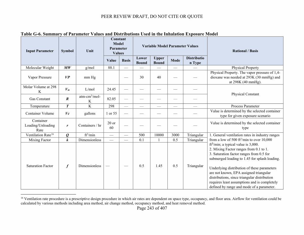
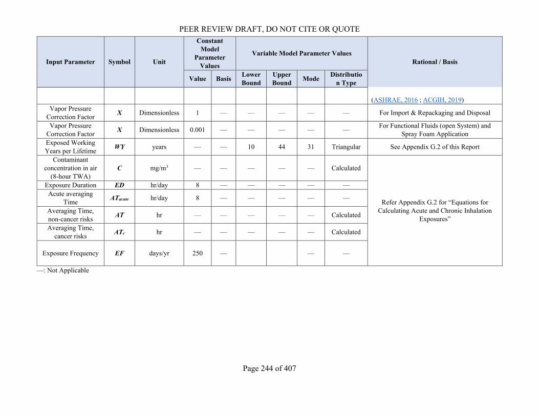
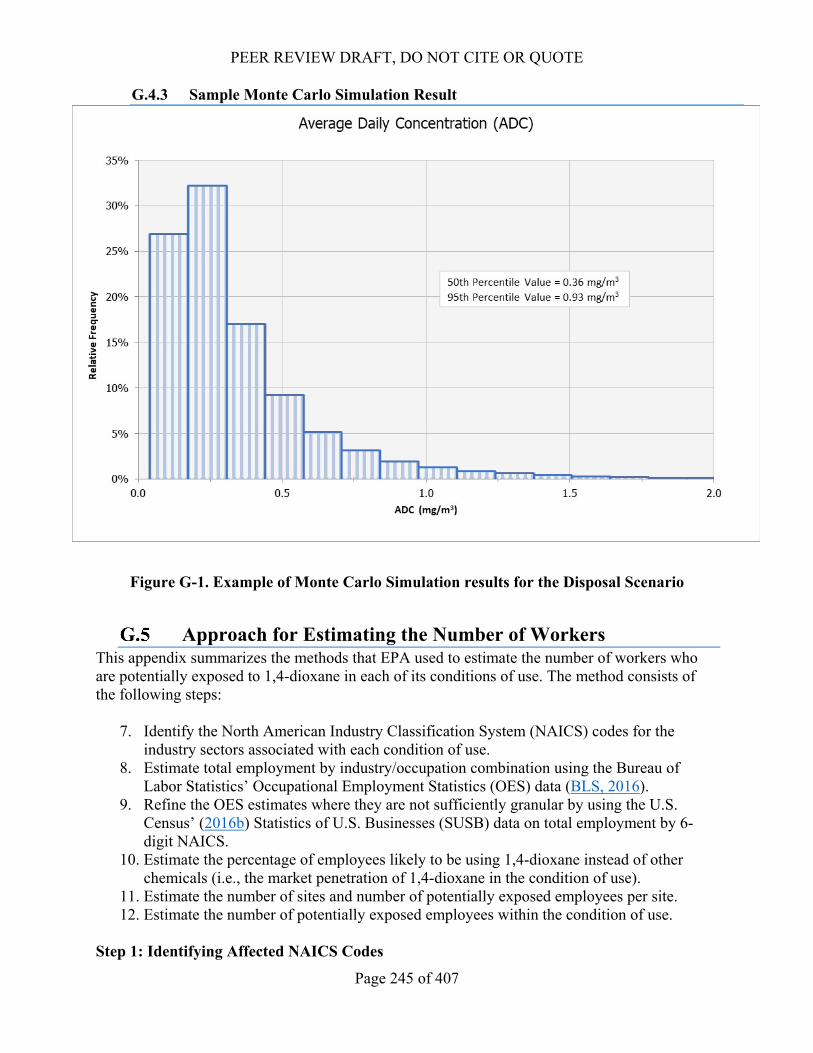
G.4.1 Model Design Equations .......................................................................................................240 G.4.2 Model Parameters .................................................................................................................242 G.4.3 Sample Monte Carlo Simulation Result ...............................................................................245
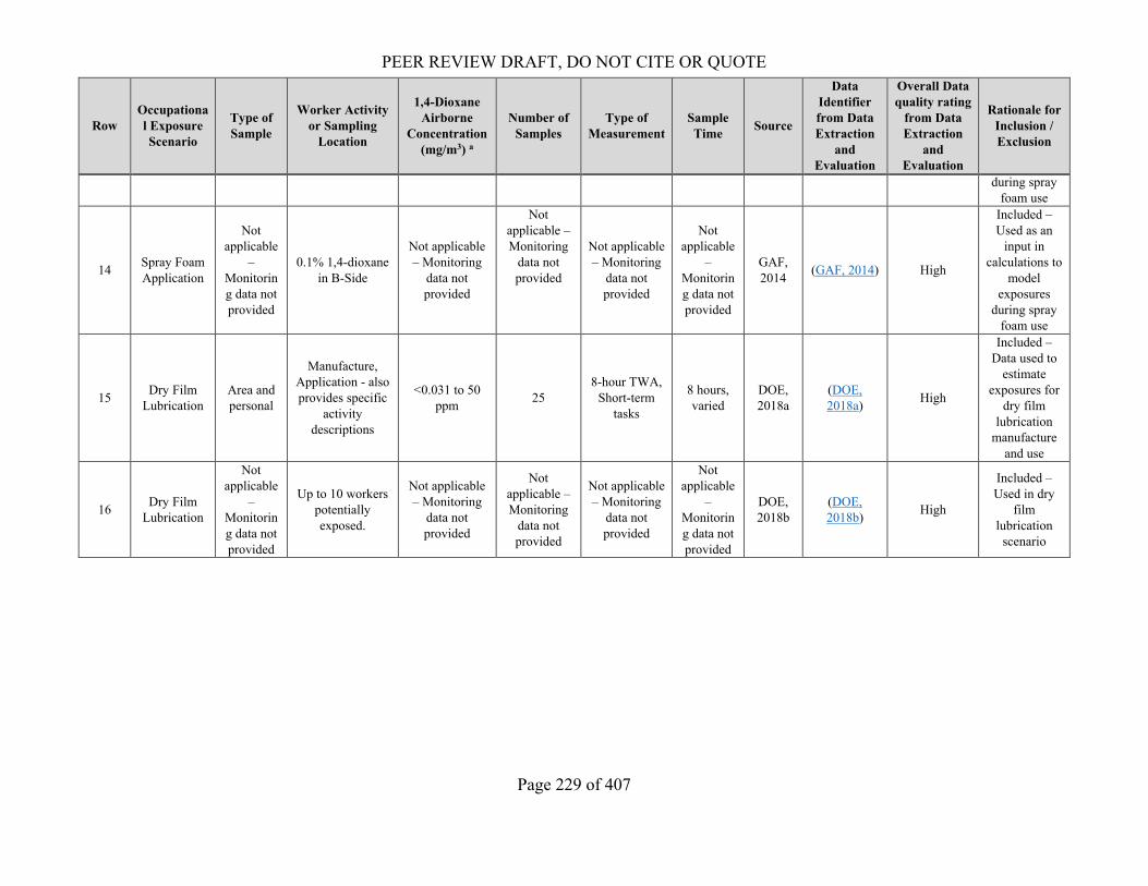
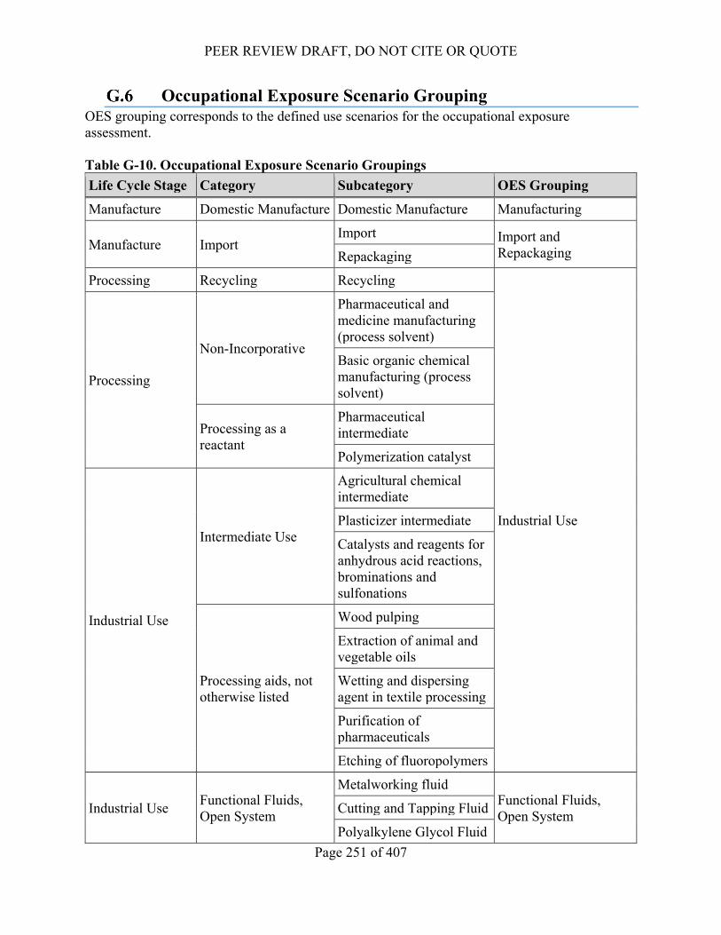
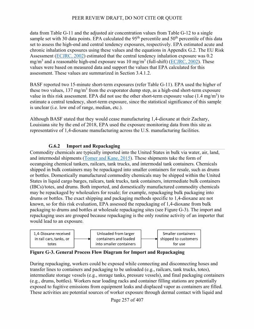
G.6.1 Manufacturing .......................................................................................................................253 G.6.2 Import and Repackaging .......................................................................................................257 G.6.3 Industrial Uses ......................................................................................................................260 G.6.4 Functional Fluids (Open System) .........................................................................................264 G.6.5 Laboratory Chemical Use .....................................................................................................268 G.6.6 Film Cement .........................................................................................................................270 G.6.7 Spray Foam Application .......................................................................................................272 G.6.8 Printing Inks (3D) .................................................................................................................276 G.6.9 Dry Film Lubricant ...............................................................................................................277 G.6.10 Disposal ................................................................................................................................281
PEER REVIEW DRAFT, DO NOT CITE OR QUOTE
5 of 407
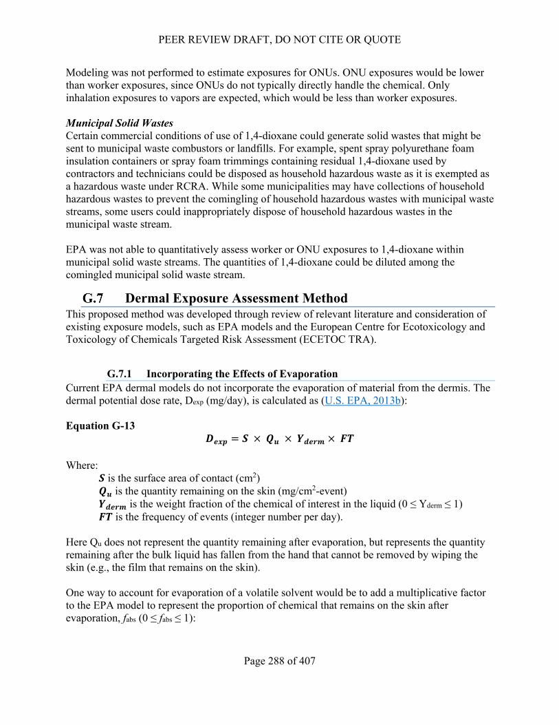
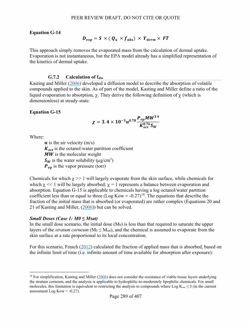
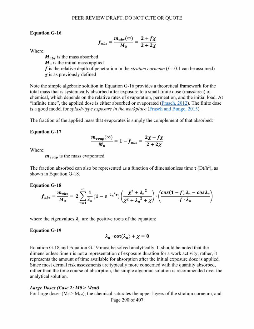
G.7.1 Incorporating the Effects of Evaporation .............................................................................288 G.7.2 Calculation of fabs ..................................................................................................................289 G.7.3 Potential for Occlusion .........................................................................................................292 G.7.4 Incorporating Glove Protection ............................................................................................293 G.7.5 Proposed Dermal Dose Equation ..........................................................................................294
HUMAN HEALTH HAZARDS .................................................................................. 295
H.1.1 Hazard and Data Evaluation Summary for Human Studies .................................................295 H.1.2 Hazard and Data Quality Evaluation Summary for Acute and Short-Term Studies ...........296 H.1.3 Hazard and Data Evaluation Summary for the Developmental Toxicity Study ...................298 H.1.4 Hazard and Data Evaluation Summary for Subchronic and Chronic Non-Cancer Studies ..298 H.1.5 Hazard and Data Evaluation Summary for Genotoxicity Studies ........................................303 H.1.6 Data Evaluation Summary for Chronic Cancer Studies .......................................................308 H.1.7 Data Evaluation Summary for Mechanistic Studies .............................................................317
LIST OF TABLES Table 2-1. Physical and Chemical Properties of 1,4-Dioxane .................................................................. 24 Table 2-2. Production Volume of 1,4-Dioxane in Chemical Data Reporting (CDR) Reporting Period
(2012 to 2015) a ................................................................................................................. 25 Table 2-3. Assessment History of 1,4-Dioxane ........................................................................................ 26 Table 2-4. Categories and Subcategories of Conditions of Use Included in the Scope of the Risk
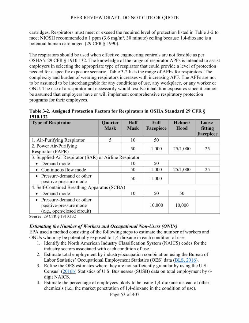
Evaluation ......................................................................................................................... 30 Table 3-1. Environmental Fate Characteristics of 1,4-Dioxane ............................................................... 44 Table 3-2. Assigned Protection Factors for Respirators in OSHA Standard 29 CFR § 1910.132 ........... 53 Table 3-3. Manufacturing Worker Exposure Data Evaluation ................................................................. 54 Table 3-4. Acute and Chronic Inhalation Exposures of Worker for Manufacturing Based on Monitoring
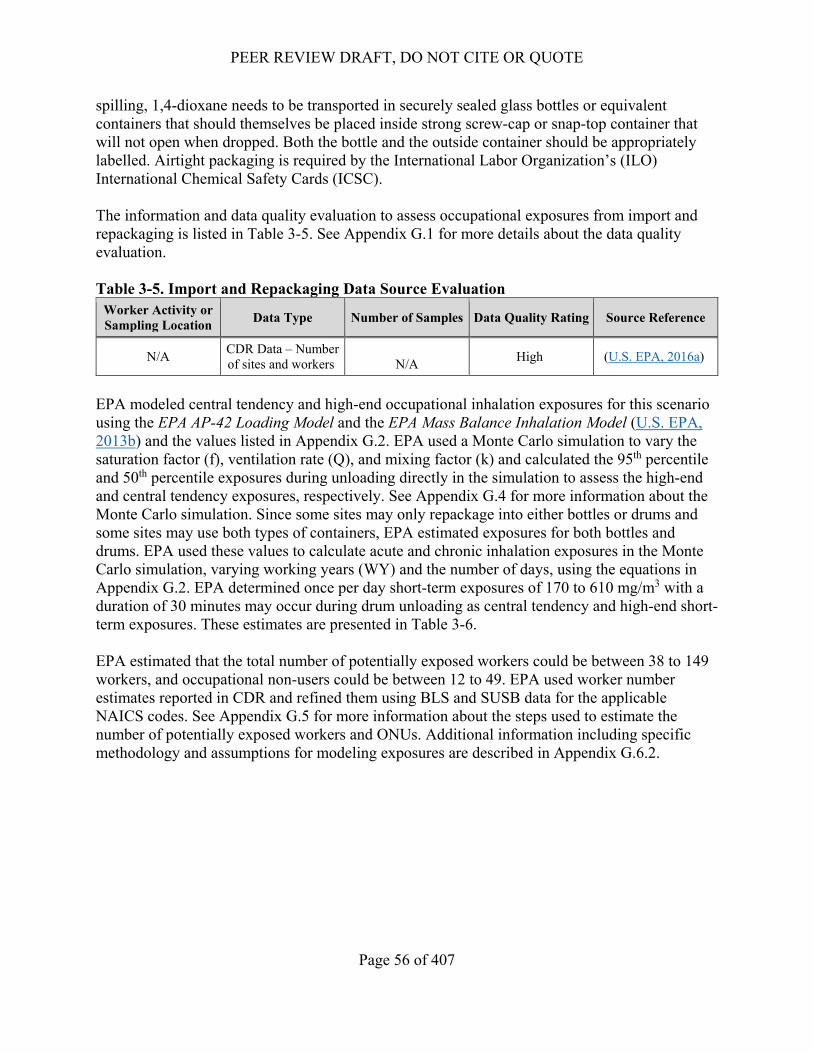
Data ................................................................................................................................... 55 Table 3-5. Import and Repackaging Data Source Evaluation ................................................................... 56 Table 3-6. Acute and Chronic Inhalation Exposures of Worker for Import and Repackaging Based on
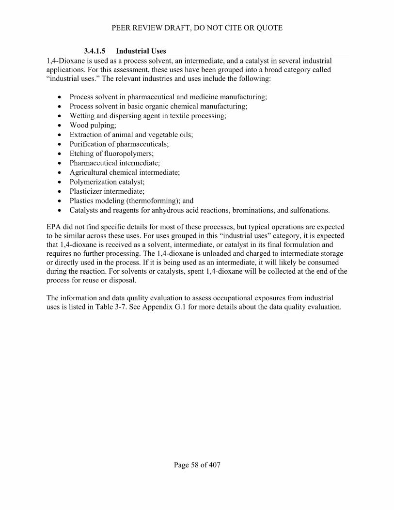
Modeling ........................................................................................................................... 57 Table 3-7. Industrial Uses Data Source Evaluation .................................................................................. 59 Table 3-8. Acute and Chronic Inhalation Exposures of Worker for Industrial Uses Based on Monitoring
Data ................................................................................................................................... 60 Table 3-9. Functional Fluids (Open System) Data Evaluation ................................................................. 61 Table 3-10. Acute and Chronic Inhalation Exposures of Worker for Open System Functional Fluids
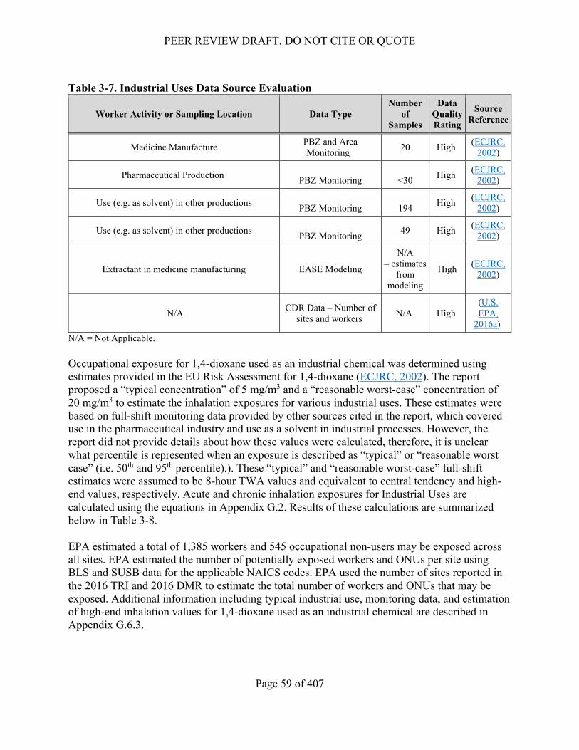
Based on Modeling ........................................................................................................... 61 Table 3-11. Acute and Chronic ONU Inhalation Exposures for Open System Functional Fluids Based on
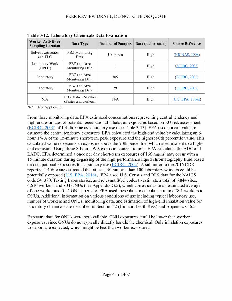
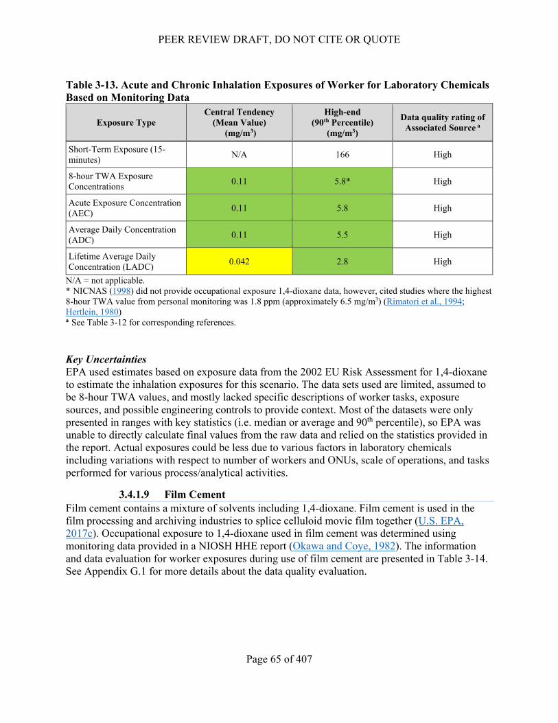
Monitoring Data ................................................................................................................ 62 Table 3-12. Laboratory Chemicals Data Evaluation ................................................................................. 64 Table 3-13. Acute and Chronic Inhalation Exposures of Worker for Laboratory Chemicals Based on
Monitoring Data ................................................................................................................ 65 Table 3-14. Film Cement Data Evaluation ............................................................................................... 66 Table 3-15. Acute and Chronic Inhalation Exposures of Worker for the Use of Film Cement Based on
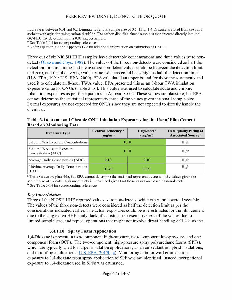
Monitoring Data ................................................................................................................ 66 Table 3-16. Acute and Chronic ONU Inhalation Exposures for the Use of Film Cement Based on
Monitoring Data ................................................................................................................ 67 Table 3-17. Spray Foam Application Data Source Evaluation ................................................................. 68 Table 3-18. Acute and Chronic Inhalation Exposures of Worker for Spray Application Based on
Modeling ........................................................................................................................... 69 Table 3-19. Acute and Chronic Non-Sprayer Workers Inhalation Exposures for Spray Applications
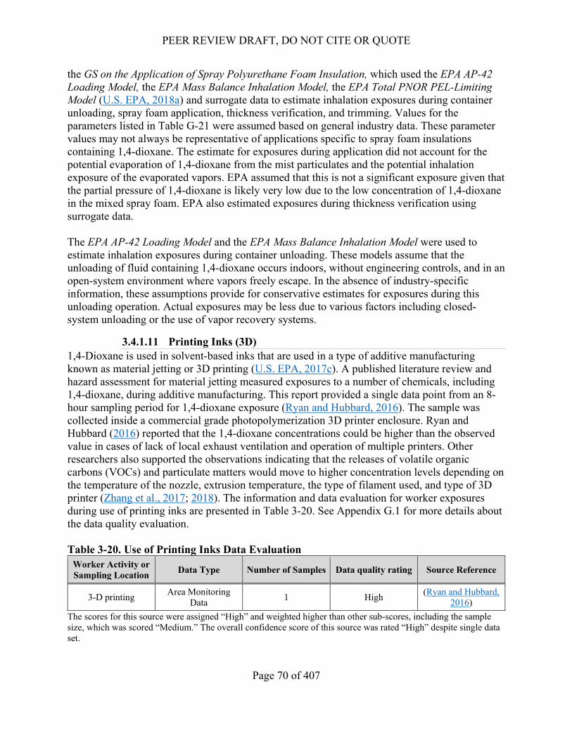
Based on Modeling ........................................................................................................... 69 Table 3-20. Use of Printing Inks Data Evaluation .................................................................................... 70 Table 3-21. Acute and Chronic Inhalation Exposures of Worker for Use of Printing Inks Based on
Monitoring Data ................................................................................................................ 71 Table 3-22. Dry Film Lubricant Data Source Evaluation ......................................................................... 72 Table 3-23. Acute and Chronic Inhalation Exposures of Workers for the Use of Dry Film Lubricant
Based on Exposure Data ................................................................................................... 72 Table 3-24. Disposal Data Source Evaluation .......................................................................................... 73 Table 3-25. Acute and Chronic Inhalation Exposures of Worker for Disposal Based on Modeling ....... 74 Table 3-26. Glove Protection Factors for Different Dermal Protection Strategies ................................... 76 Table 3-27. Estimated Dermal Absorbed Dose1 (mg/day) for Workers in All Conditions of Use ........... 79
PEER REVIEW DRAFT, DO NOT CITE OR QUOTE
8 of 407
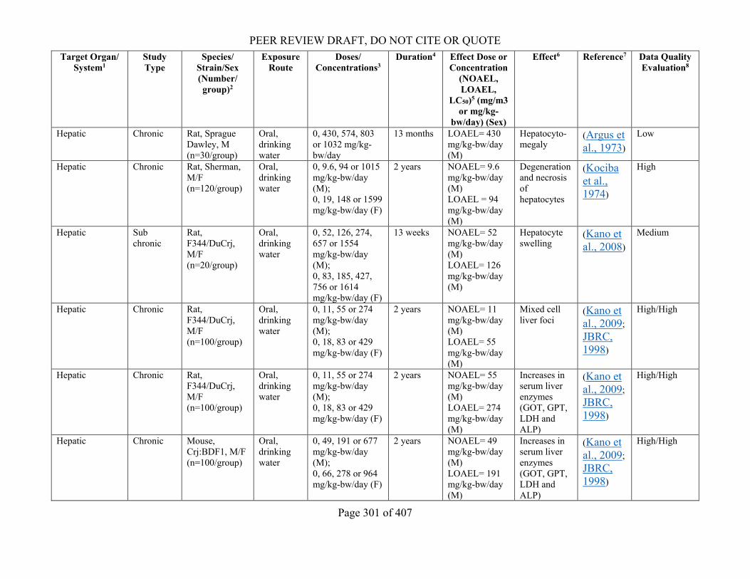
Table 4-1. Acceptable Studies Evaluated for Toxicity of 1,4-Dioxane Following Acute or Short-term Exposurea .......................................................................................................................... 87
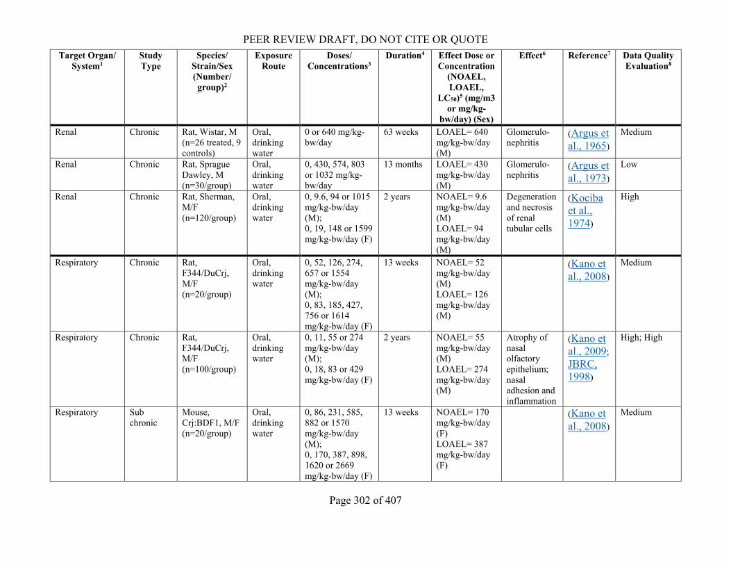
Table 4-2. Acceptable Studies Evaluated for Non-Cancer Subchronic or Chronic Toxicity of 1,4-Dioxane Following Inhalation Exposure .......................................................................... 88
Table 4-3. Acceptable Subchronic and Chronic Studies Evaluated for Non-Cancer Toxicity of 1,4-Dioxane Following Oral Exposure ................................................................................... 90
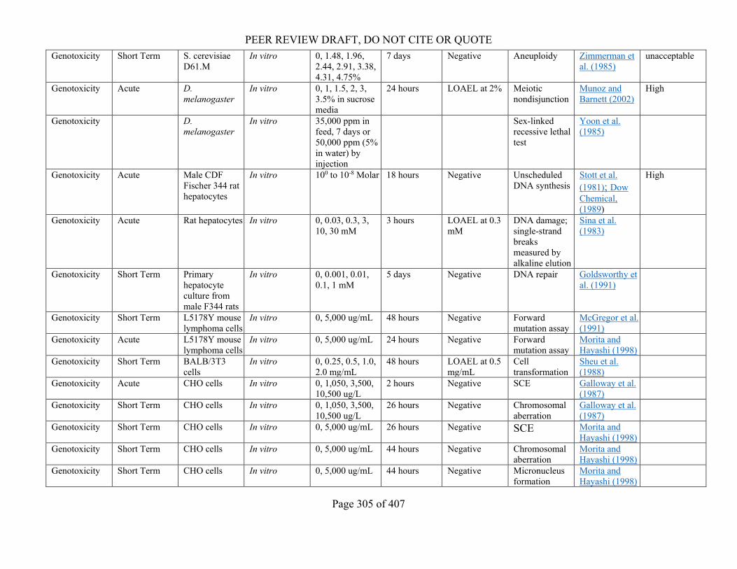
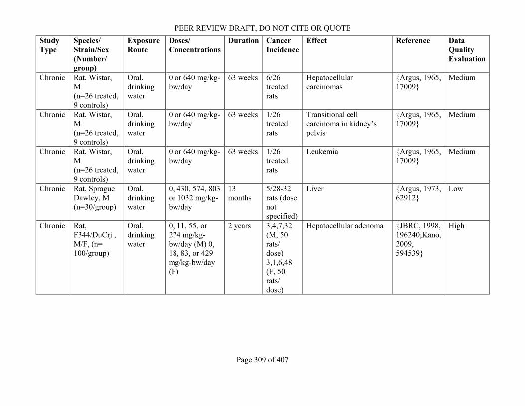
Table 4-4. Acceptable New Studies Evaluated for Genetic Toxicity of 1,4-Dioxane .............................. 93 Table 4-5. Studies Evaluated for Cancer Following Inhalation Exposure to 1,4-Dioxane ....................... 96 Table 4-6. Studies Evaluated for Cancer Following Oral and Inhalation Exposure to 1,4-Dioxane ........ 97 Table 4-7A. Incidence of carcinogenic and non-carcinogenic lesions reported at each dose level in a two
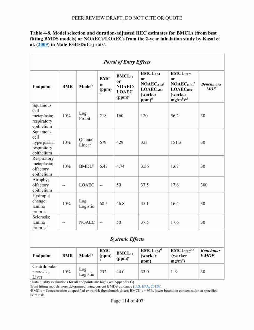
year inhalation study in rats ............................................................................................ 102 Table 4-8. Model selection and duration-adjusted HEC estimates for BMCLs (from best fitting BMDS
models) or NOAECs/LOAECs from the 2-year inhalation study by Kasai et al. (2009) in Male F344/DuCrj ratsa. ................................................................................................... 114
Table 4-9. Dose-response modeling summary results for male rat tumors associated with inhalation exposure to 1,4-dioxane for 2 years ................................................................................ 116
Table 4-10. Dose-response modeling summary results for oral non-cancer liver, kidney, and nasal effects and route-to-route extrapolated applied dermal HEDs ................................................... 121
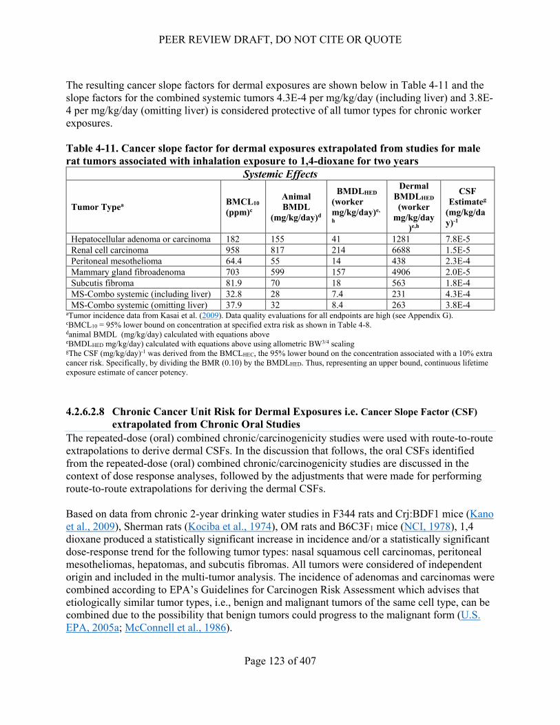
Table 4-11. Cancer slope factor for dermal exposures extrapolated from studies for male rat tumors associated with inhalation exposure to 1,4-dioxane for 2 years ..................................... 123
Table 4-12. Dose-response modeling summary results for oral CSFs and route-to-route extrapolated dermal CSFs. ................................................................................................................... 126
Table 4-13. Summary of Hazard Identification and Dose-Response Values ......................................... 128 Table 5-1. Concentrations of Concern (COCs) for Environmental Toxicity .......................................... 130 Table 5-2. Calculated Risk Quotients (RQs) for 1,4-Dioxane ................................................................ 131 Table 5-3. Summary of Parameters for Risk Characterization ............................................................... 132 Table 5-4. MOE for Acute/Short-term Inhalation Exposures; Benchmark MOE = 300 ........................ 136 Table 5-5. Chronic Inhalation Exposure Risk to Workers: Non-Cancer; benchmark MOE=30 ............ 137 Table 5-6. Inhalation Exposure Risk to Occupational Non-Users: Non-Cancer; Benchmark MOE = 30
......................................................................................................................................... 138 Table 5-7. Inhalation Exposure Risk Estimates to Workers: Cancer; Benchmark Risk = 1 in 104 ........ 140 Table 5-8. Inhalation Exposures to Occupational Non-Users: Cancer; Benchmark Risk = 1 in 104 ..... 141 Table 5-9. Dermal Exposure Risk Estimates to Workers: for Acute/Short-term Exposures Non-Cancer;
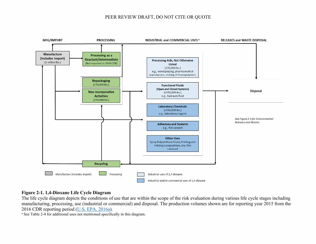
Benchmark MOE = 300 .................................................................................................. 142 Table 5-10. Dermal Exposure Risk Estimates to Workers: Non-Cancer; Benchmark MOE = 30 ......... 144 Table 5-11. Dermal Exposure Risk Estimates to Workers: Cancer ........................................................ 145 Table 6-1. Risk Determination by Conditions of Use…………………………………………………..158 LIST OF FIGURES Figure 2-1. 1,4-Dioxane Life Cycle Diagram ........................................................................................... 29 Figure 2-2. 1,4-Dioxane Conceptual Model for Industrial and Commercial Activities and Uses: Potential
Exposures and Hazards ..................................................................................................... 34 Figure 2-3. 1,4-Dioxane Conceptual Model for Environmental Releases and Wastes: Potential
Exposures and Hazards ..................................................................................................... 35 Figure 2-4. Literature Flow Diagram for Environmental Fate and Transport Data Sources .................... 38 Figure 2-5. Literature Flow Diagram for Engineering Releases and Occupational Exposure Data
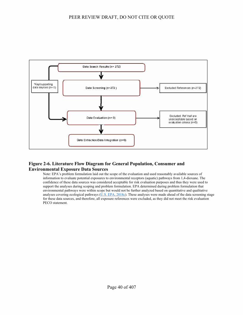
Figure 2-6. Literature Flow Diagram for General Population, Consumer and Environmental Exposure Data Sources ..................................................................................................................... 40
Figure 2-7. Literature Flow Diagram for Environmental Hazard Data Sources ....................................... 41 Figure 2-8. Literature Flow Diagram for Human Health Hazard Data Sources ....................................... 42 Figure 4-1. EPA Approach to Human Health Hazard Identification and Dose-Response for 1,4-Dioxane
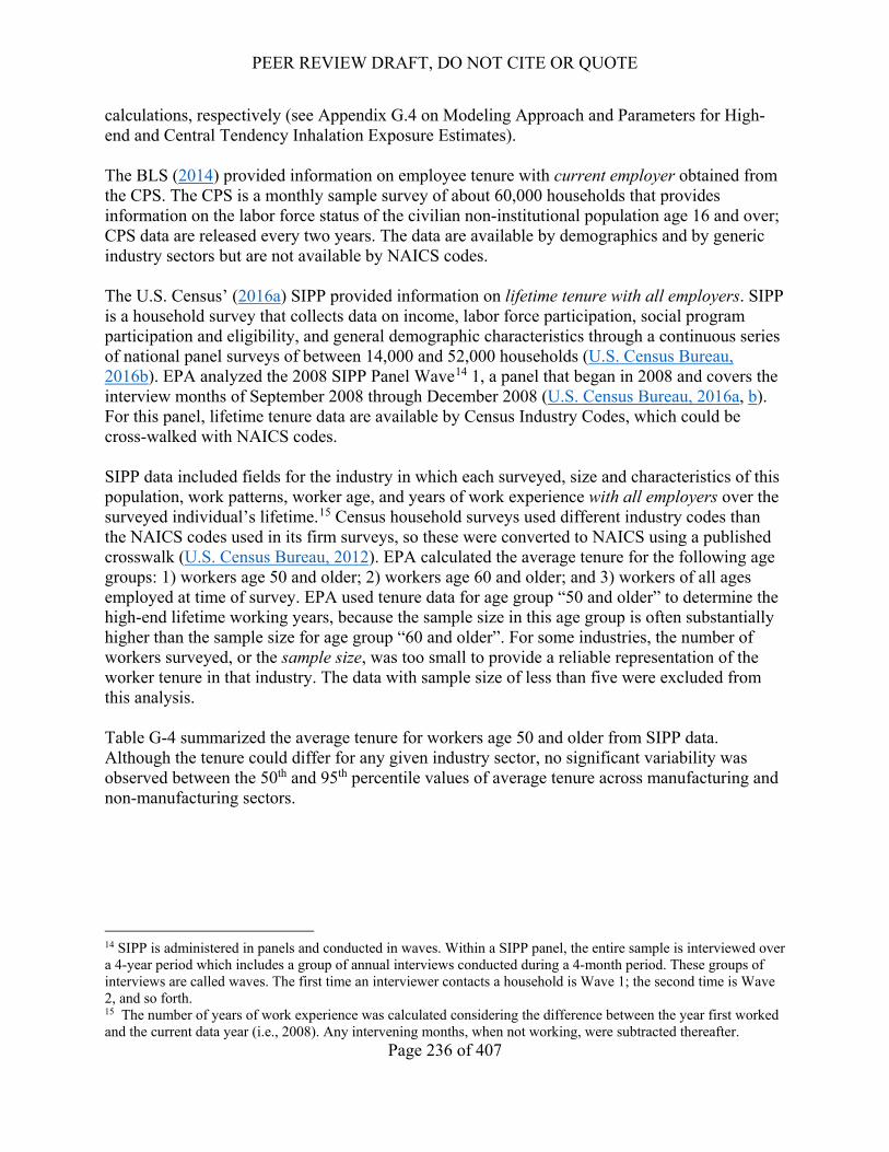
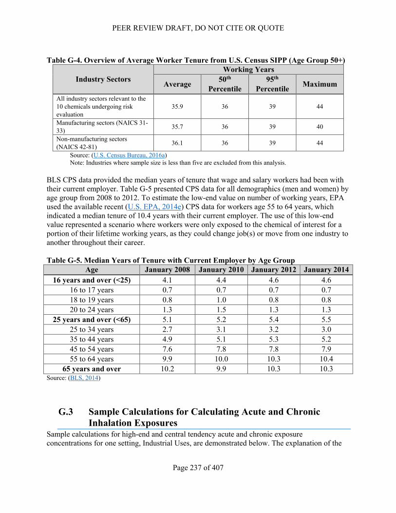
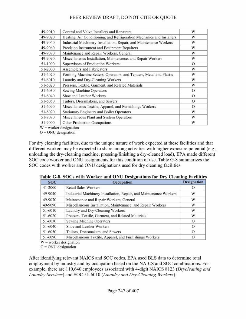
........................................................................................................................................... 81 Figure 4-2. 1,4-Dioxane Metabolism Pathways ....................................................................................... 84 LIST OF APPENDIX TABLES Table A-1. Federal Laws and Regulations .............................................................................................. 190 Table A-2. State Laws and Regulations .................................................................................................. 195 Table A-3. Regulatory Actions by other Governments and Tribes ........................................................ 196 Table B-1. Industrial and Commercial Occupational Exposure Scenarios for 1,4-Dioxane .................. 198 Table B-2. Environmental Releases and Wastes Exposure Scenarios for 1,4-Dioxane ......................... 208 Table E-1. Summary of 1,4-Dioxane TRI Releases to the Environment in 2015 (lbs) .......................... 214 Table E-2. Facility Selection Characterization ....................................................................................... 215 Table E-3. Summary of Modeled Surface Water Concentrations for DMR Facilities ........................... 217 Table E-4. Summary of Modeled Surface Water Concentrations for TRI Facilities .............................. 219 Table F-1. Acceptable acute aquatic toxicity studies that were evaluated for of 1,4-Dioxane ............... 221 Table F-2. Acceptable chronic aquatic toxicity studies that were evaluated for of 1,4-Dioxane ........... 223 Table G-1. Summary of Inhalation Monitoring Data Sources Specific to 1,4-Dioxane ......................... 226 Table G-2. Summary of Cross-Cutting Data Sources ............................................................................. 230 Table G-3. Representative Worker Exposure Durations Considered for Risk Assessments .................. 234 Table G-4. Overview of Average Worker Tenure from U.S. Census SIPP (Age Group 50+) ............... 237 Table G-5. Median Years of Tenure with Current Employer by Age Group ......................................... 237 Table G-6. Summary of Parameter Values and Distributions Used in the Inhalation Exposure Model 243 Table G-7. SOCs with Worker and ONU Designations for All Conditions of Use Except Dry Cleaning
......................................................................................................................................... 246 Table G-8. SOCs with Worker and ONU Designations for Dry Cleaning Facilities ............................. 247 Table G-9. Estimated Number of Potentially Exposed Workers and ONUs under NAICS 812320 ...... 248 Table G-10. Occupational Exposure Scenario Groupings ...................................................................... 251 Table G-11 2017 1,4-Dioxane Production Monitoring Data (BASF, 2017) .......................................... 255 Table G-12. 2007-2011 1,4-Dioxane Production Monitoring Data (BASF, 2016) ................................ 255 Table G-13. 2016 CDR Data and Assumed Container Types for Repackaging ..................................... 259 Table G-14. Number of Totes and Containers per Site .......................................................................... 259 Table G-15. Industrial Use NAICS Codes .............................................................................................. 262 Table G-16. DoD and 2002 EU Risk Assessment Industrial Use Inhalation Exposure Data ................. 263 Table G-17. 1997 NIOSH HHE PBZ and Area Sampling Data for Metalworking Fluids ..................... 266 Table G-18. 2011 ESD on Metalworking Fluids Inhalation Exposure Estimates .................................. 268 Table G-19. Monitoring Data for Laboratory Chemicals ....................................................................... 270 Table G-20. NIOSH HHE PBZ and Area Samples for Film Cement Use ............................................. 272 Table G-21. Values Used for Daily Site Use Rate for SPF Application ................................................ 274 Table G-22. Estimated Activity Exposure Durations ............................................................................. 275 Table G-23. PBZ Task and TWA Monitoring Data for Dry Film Lubricant Manufacture and Spray
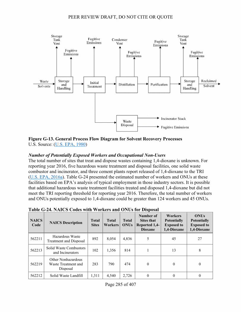
Application at KCNSC ................................................................................................... 279 Table G-24. NAICS Codes with Workers and ONUs for Disposal ........................................................ 285 Table G-25. 2016 TRI Off-Site Transfers for 1,4-Dioxane .................................................................... 287
PEER REVIEW DRAFT, DO NOT CITE OR QUOTE
10 of 407
Table G-26. Estimated Fraction Evaporated and Absorbed (fabs) using Equation G-20 ....................... 291 Table G-27. Exposure Control Efficiencies and Protection Factors for Different Dermal Protection
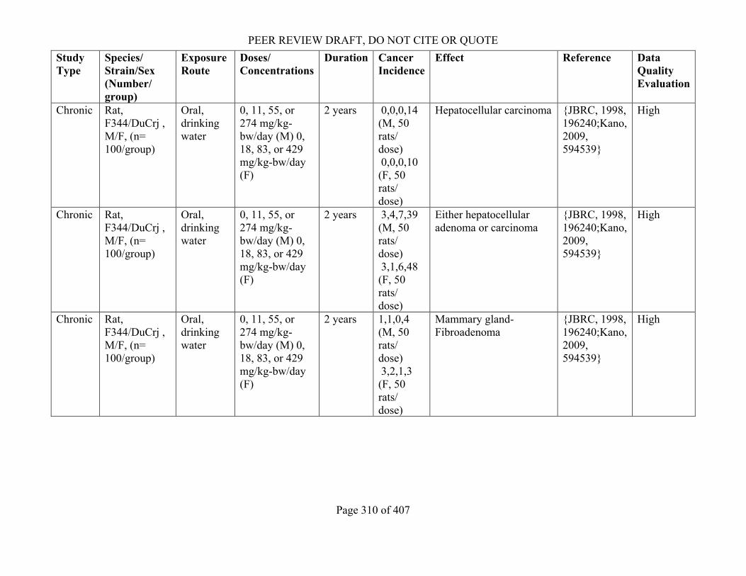
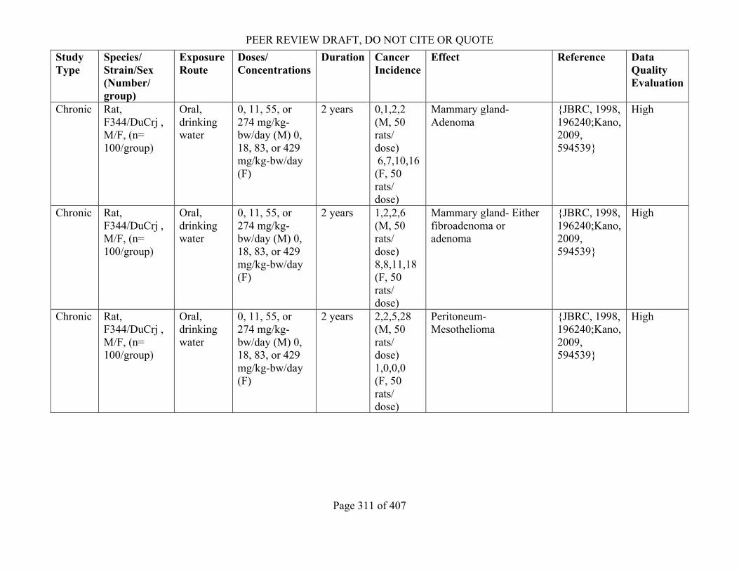
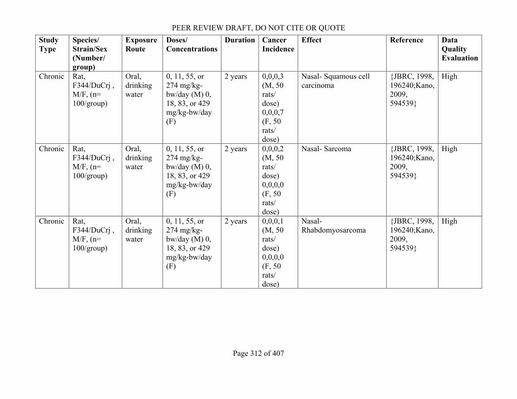
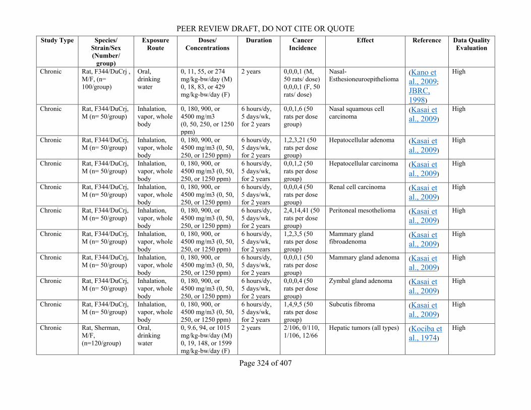
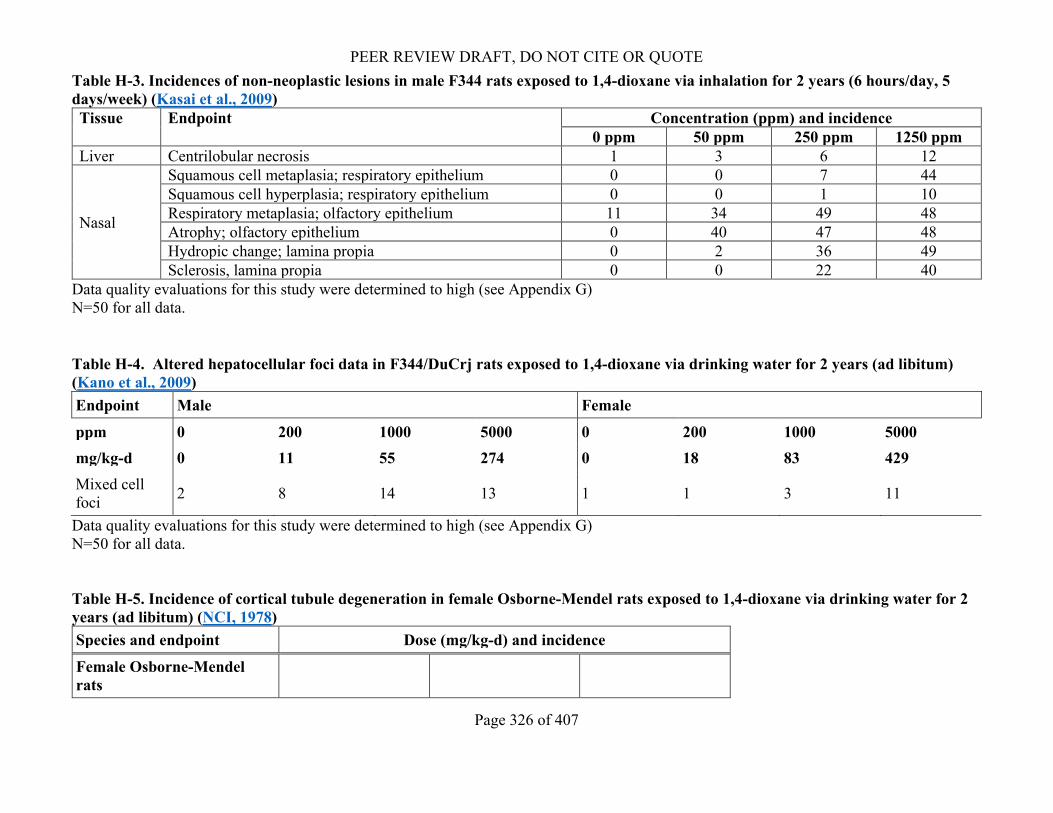
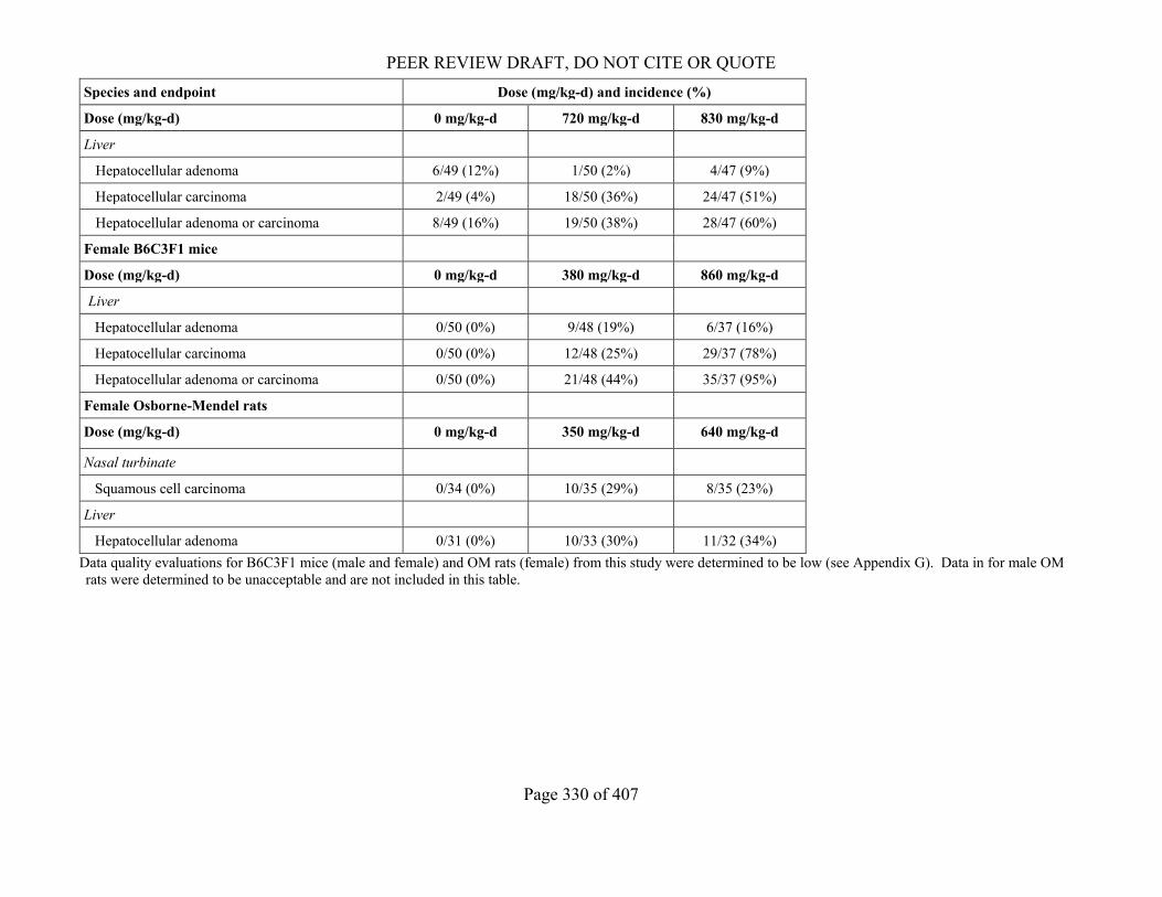
Strategies from ECETOC TRA v3 ................................................................................. 293 Table H-1. Summary of Mechanistic Data for 1,4-Dioxane ................................................................... 317 Table H-2. Cancer Incidence for 1,4-Dioxane Studies with Acceptable Data Quality Ratings1 ............ 322 Table H-3. Incidences of non-neoplastic lesions in male F344 rats exposed to 1,4-dioxane via inhalation
for 2 years (6 hours/day, 5 days/week) (Kasai et al., 2009) ............................................ 326 Table H-4. Altered hepatocellular foci data in F344/DuCrj rats exposed to 1,4-dioxane via drinking
water for 2 years (ad libitum) (Kano et al., 2009) .......................................................... 326 Table H-5. Incidence of cortical tubule degeneration in female Osborne-Mendel rats exposed to 1,4-
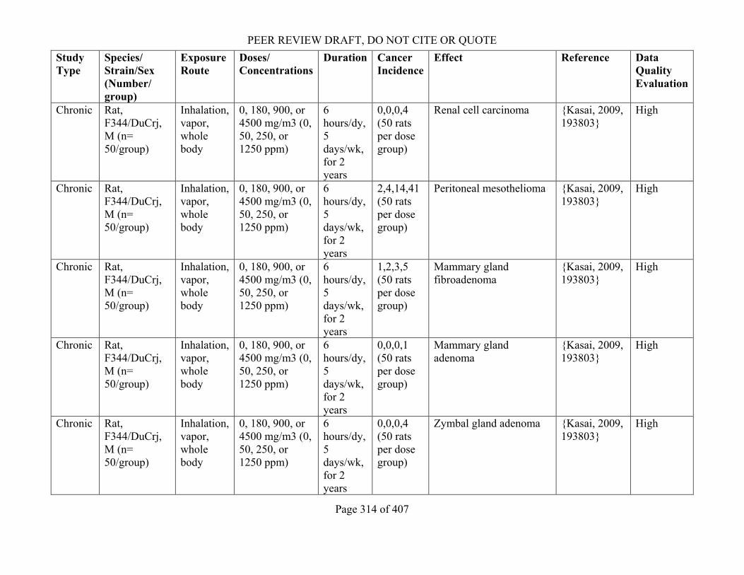
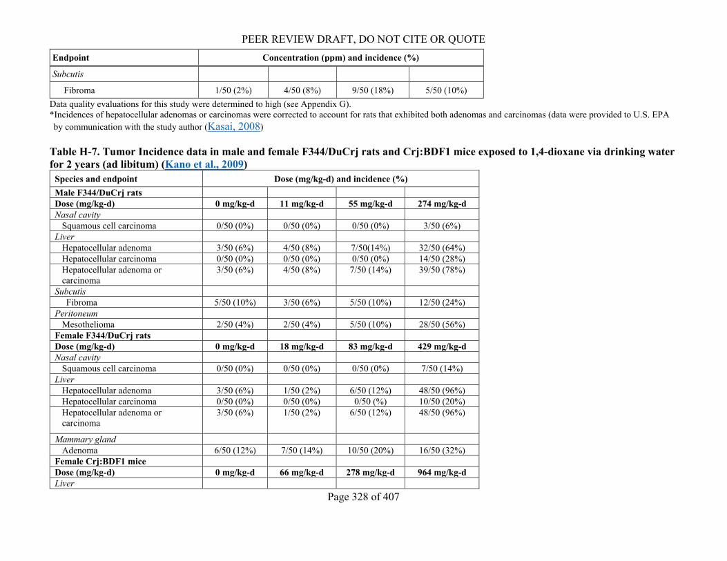
dioxane via drinking water for 2 years (ad libitum) (NCI, 1978) ................................... 326 Table H-6. Tumor incidence data in male F344 rats exposed to 1,4-dioxane via inhalation for 2 years (6
hours/day, 5 days/week) (Kasai et al., 2009) .................................................................. 327 Table H-7. Tumor Incidence data in male and female F344/DuCrj rats and Crj:BDF1 mice exposed to
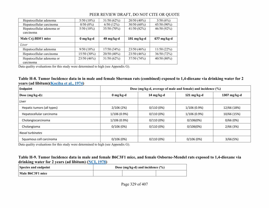
1,4-dioxane via drinking water for 2 years (ad libitum) (Kano et al., 2009) .................. 328 Table H-8. Tumor Incidence data in in male and female Sherman rats (combined) exposed to 1,4-
dioxane via drinking water for 2 years (ad libitum)(Kociba et al., 1974) ...................... 329 Table H-9. Tumor Incidence data in male and female B6C3F1 mice, and female Osborne-Mendel rats
exposed to 1,4-dioxane via drinking water for 2 years (ad libitum) (NCI, 1978) .......... 329 Table I-1. Summary of BMD Modeling Results for Centrilobular necrosis of the liver in male
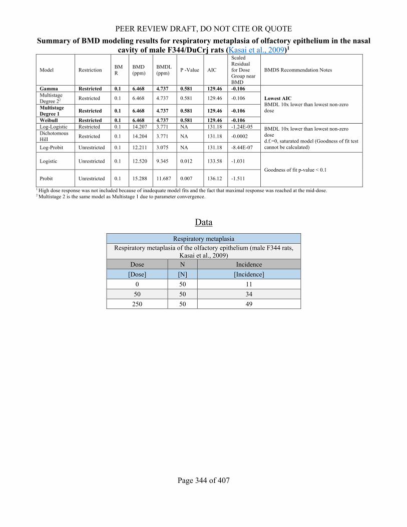
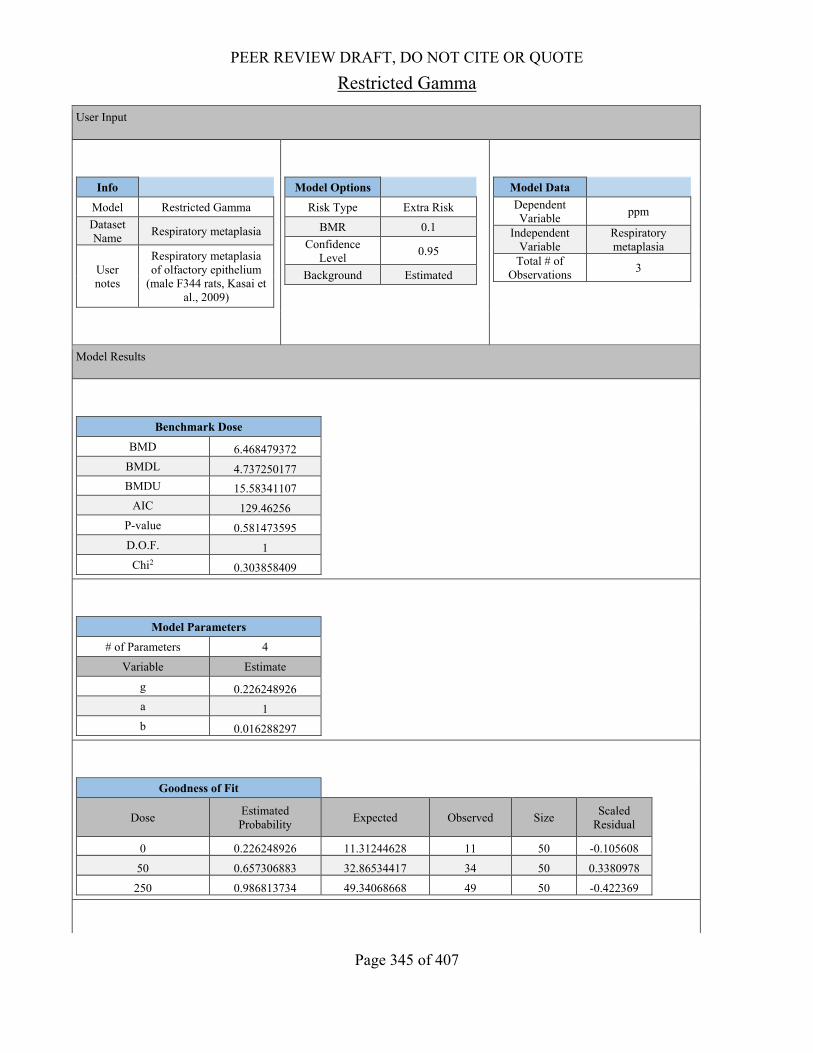
F344/DuCrj rats (Kasai et al., 2009) ............................................................................... 335 Table I-2. Summary of BMD Modeling Results for Squamous cell metaplasia of respiratory epithelium
in male F433/DuCrj rats (Kasai et al., 2009) .................................................................. 338 Table I-3. Summary of BMD Modeling Results for Squamous cell hyperplasia of respiratory epithelium
in male F433/DuCrj rats (Kasai et al., 2009) .................................................................. 340 Table I-4. Summary of BMD Modeling Results for Hydropic change (lamina propria) (Kasai et al.,
2009) ............................................................................................................................... 351 Table I-5. Summary of BMD Modeling Results for Nasal cavity squamous cell carcinoma (male
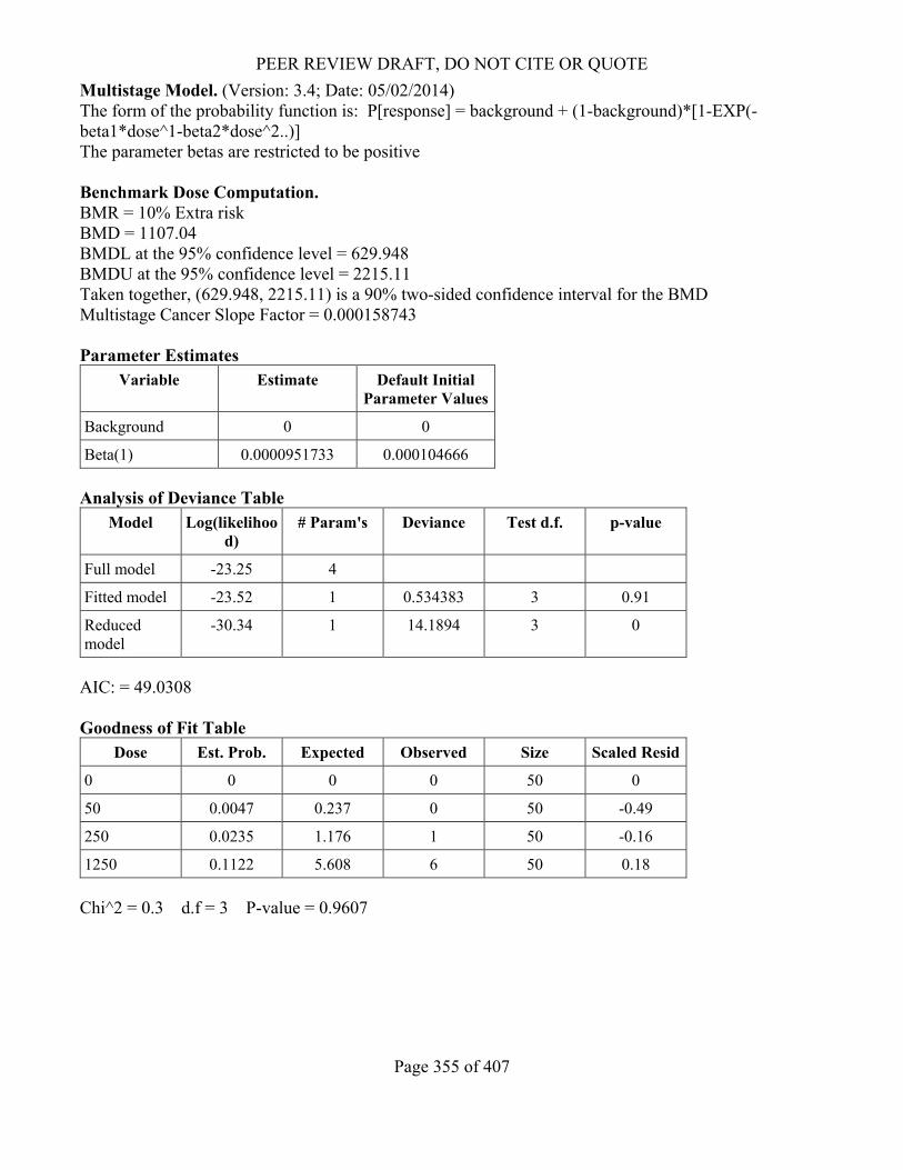
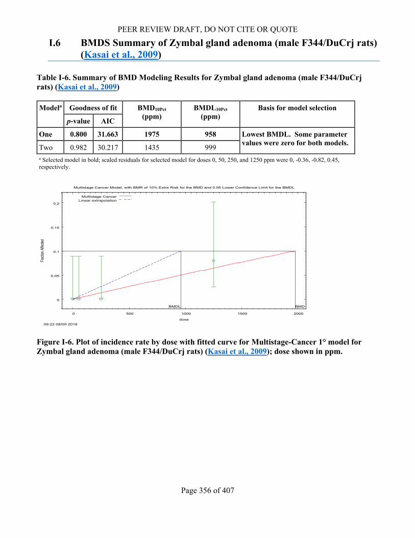
F344/DuCrj rats) (Kasai et al., 2009) .............................................................................. 354 Table I-6. Summary of BMD Modeling Results for Zymbal gland adenoma (male F344/DuCrj rats)
(Kasai et al., 2009) .......................................................................................................... 356 Table I-7. Summary of BMD Modeling Results for Hepatocellular adenoma or carcinoma (male
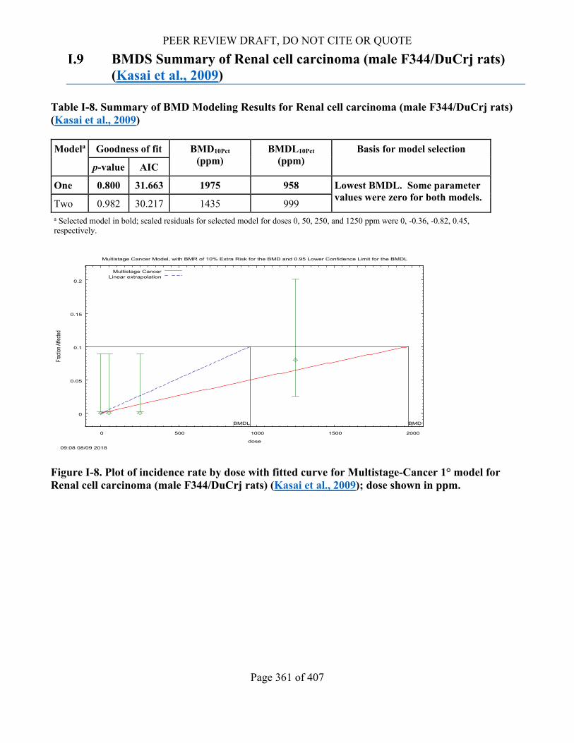
F344/DuCrj rats) (Kasai et al., 2009) .............................................................................. 358 Table I-8. Summary of BMD Modeling Results for Renal cell carcinoma (male F344/DuCrj rats) (Kasai
et al., 2009) ..................................................................................................................... 361 Table I-9. Summary of BMD Modeling Results for Peritoneal mesothelioma (male F344/DuCrj rats)
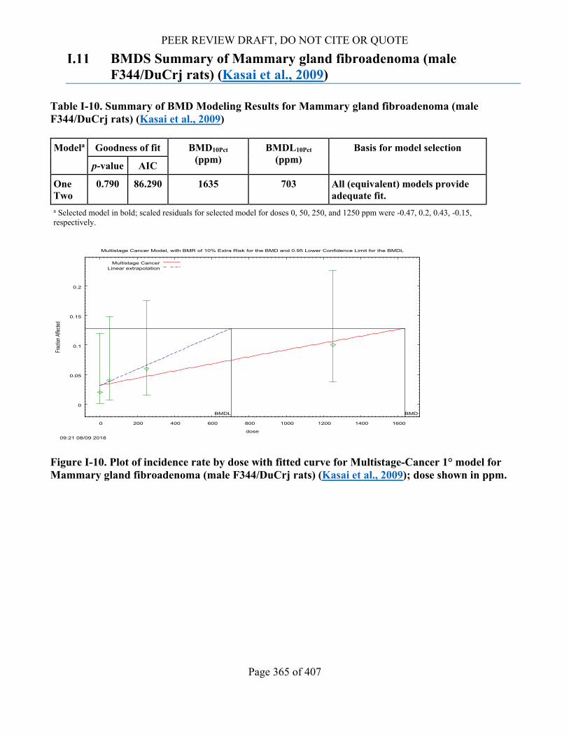
(Kasai et al., 2009) .......................................................................................................... 363 Table I-10. Summary of BMD Modeling Results for Mammary gland fibroadenoma (male F344/DuCrj
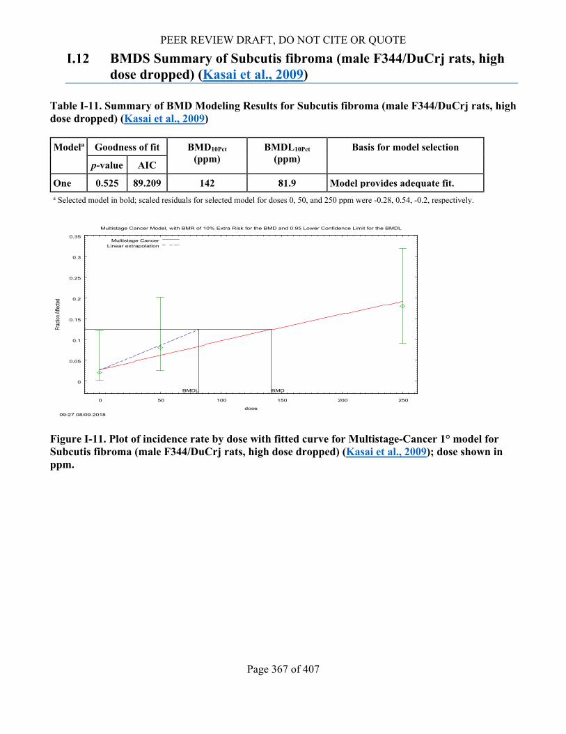
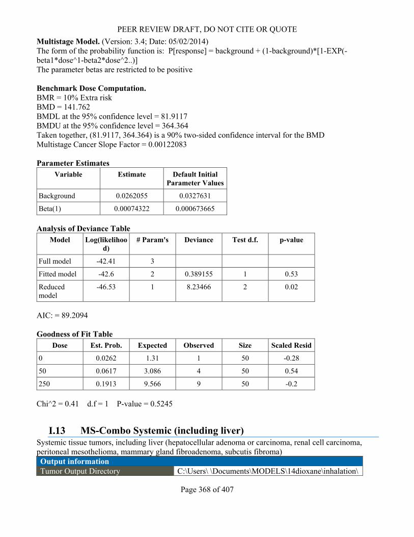
rats) (Kasai et al., 2009) .................................................................................................. 365 Table I-11. Summary of BMD Modeling Results for Subcutis fibroma (male F344/DuCrj rats, high dose
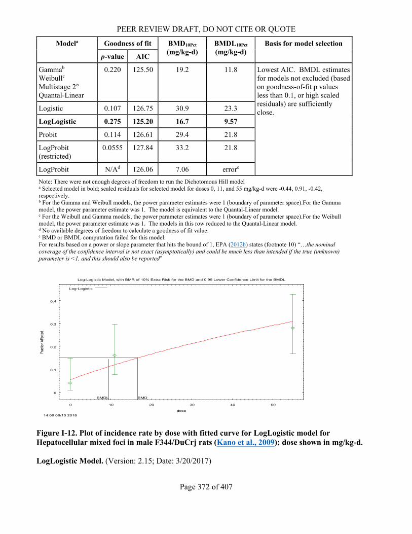
dropped) (Kasai et al., 2009)........................................................................................... 367 Table I-12. Summary of BMD Modeling Results for Hepatocellular mixed foci in male F344/DuCrj rats
(Kano et al., 2009) .......................................................................................................... 371 Table I-13. Summary of BMD Modeling Results for Cortical tubule degeneration in female OM rats
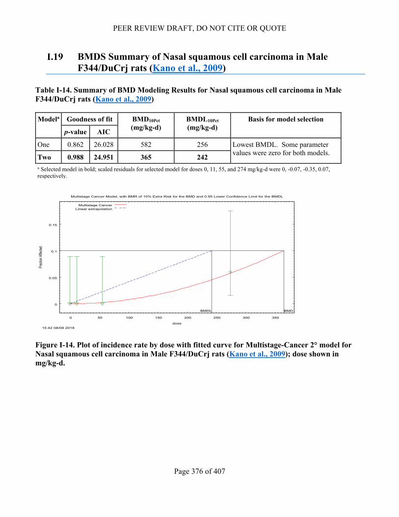
(NCI, 1978) ..................................................................................................................... 374 Table I-14. Summary of BMD Modeling Results for Nasal squamous cell carcinoma in Male
F344/DuCrj rats (Kano et al., 2009) ............................................................................... 376
PEER REVIEW DRAFT, DO NOT CITE OR QUOTE
11 of 407
Table I-15. Summary of BMD Modeling Results for Peritoneum mesothelioma in Male F344/DuCrj rats (Kano et al., 2009) .......................................................................................................... 378
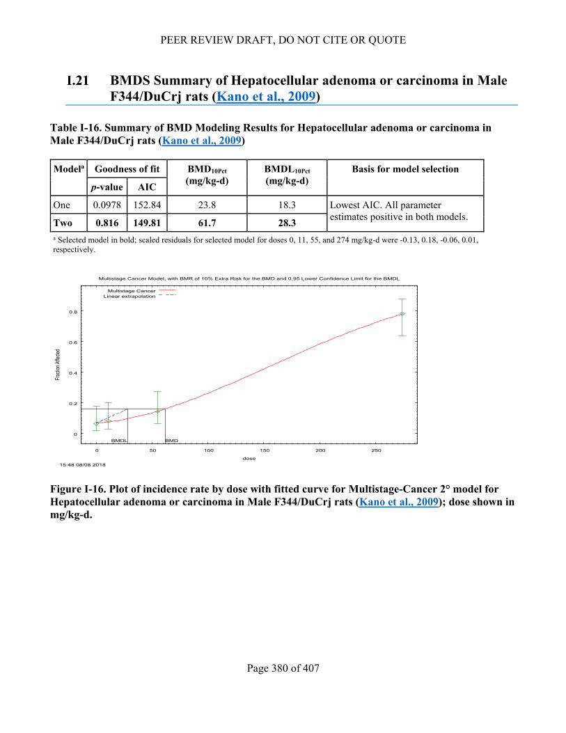
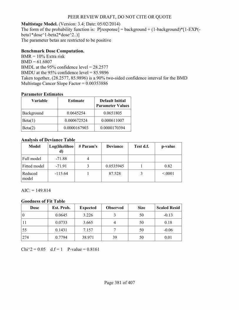
Table I-16. Summary of BMD Modeling Results for Hepatocellular adenoma or carcinoma in Male F344/DuCrj rats (Kano et al., 2009) ............................................................................... 380
Table I-17. Summary of BMD Modeling Results for Subcutis fibroma in Male F344/DuCrj rats (Kano et al., 2009) ......................................................................................................................... 382
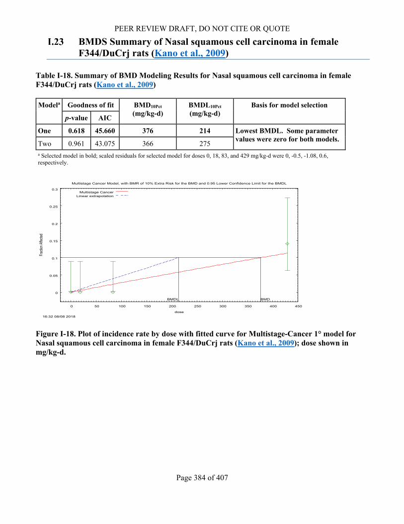
Table I-18. Summary of BMD Modeling Results for Nasal squamous cell carcinoma in female F344/DuCrj rats (Kano et al., 2009) ............................................................................... 384
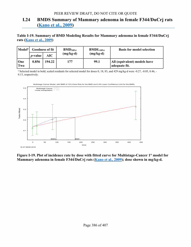
Table I-19. Summary of BMD Modeling Results for Mammary adenoma in female F344/DuCrj rats (Kano et al., 2009) .......................................................................................................... 386
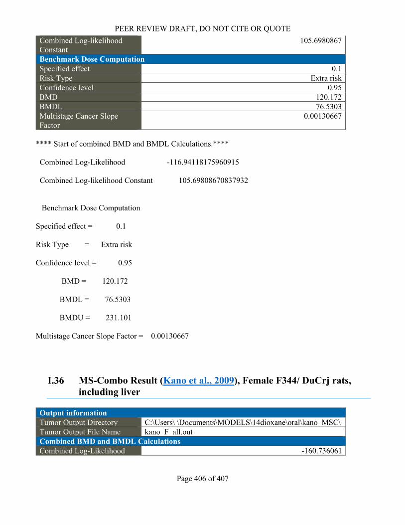
Table I-20. Summary of BMD Modeling Results for Hepatocellular adenomas or carcinomas female F344/DuCrj rats (Kano et al., 2009) ............................................................................... 388
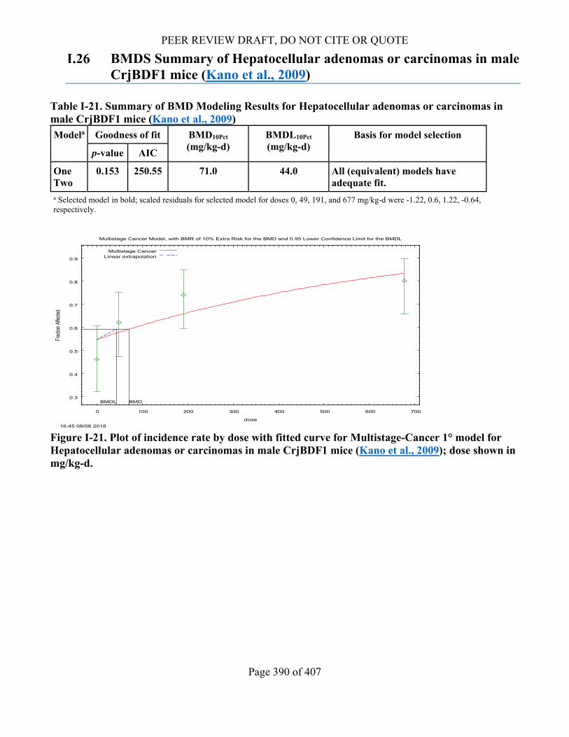
Table I-21. Summary of BMD Modeling Results for Hepatocellular adenomas or carcinomas in male CrjBDF1 mice (Kano et al., 2009) .................................................................................. 390
Table I-22. Summary of BMD Modeling Results for Nasal cavity tumors in Sherman rats (Kociba et al., 1974) ............................................................................................................................... 392
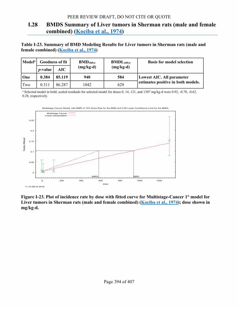
Table I-23. Summary of BMD Modeling Results for Liver tumors in Sherman rats (male and female combined) (Kociba et al., 1974) ..................................................................................... 394
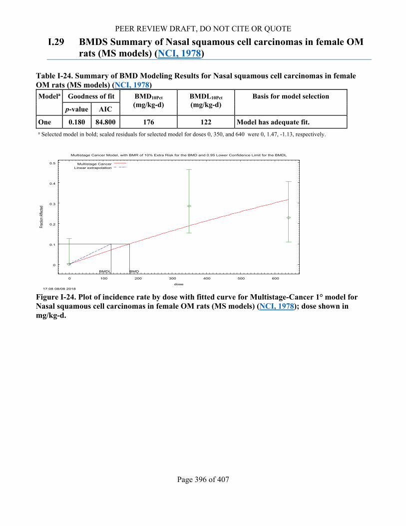
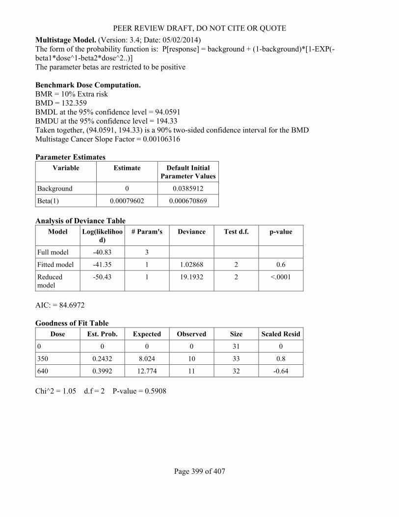
Table I-24. Summary of BMD Modeling Results for Nasal squamous cell carcinomas in female OM rats (MS models) (NCI, 1978) ............................................................................................... 396
Table I-25. Summary of BMD Modeling Results for Hepatocellular adenoma in female OM rats (NCI, 1978) ............................................................................................................................... 398
Table I-26. Summary of BMD Modeling Results for Hepatocellular adenomas or carcinomas in male B6C3F1 mice (NCI, 1978) .............................................................................................. 400
Table I-27. Summary of BMD Modeling Results for Hepatocellular adenomas or carcinomas in female B6C3F1 mice (NCI, 1978) .............................................................................................. 402
LIST OF APPENDIX FIGURES Figure D 1. EPI Suite™ welcome screen set up for 1,4-dioxane model run………………………… 211 Figure G-1. Example of Monte Carlo Simulation results for the Disposal Scenario ............................. 245 Figure G-2. Generic Manufacturing Process Flow Diagram .................................................................. 253 Figure G-3. General Process Flow Diagram for Import and Repackaging ............................................. 257 Figure G-4. Generic Industrial Use Process Flow Diagram ................................................................... 260 Figure G-5. Process Flow Diagram for Open System Functional Fluids ............................................... 265 Figure G-6. General Laboratory Use Process Flow Diagram ................................................................. 269 Figure G-7. Process Flow Diagram for Film Cement Application ......................................................... 271 Figure G-8. Process Flow Diagram for Spray Application..................................................................... 273 Figure G-9. Process Flow Diagram for Printing Inks (3D) .................................................................... 276 Figure G-10. Process Flow Diagram for Dry Film Lubricant in Nuclear Weapon Applications ........... 278 Figure G-11. Typical Waste Disposal Process ....................................................................................... 282 Figure G-12. Typical Industrial Incineration Process ............................................................................. 283 Figure G-13. General Process Flow Diagram for Solvent Recovery Processes ..................................... 285 Figure H-1. Literature Flow Diagram for Human Health Hazard .......................................................... 295 Figure I-1. Plot of incidence rate by dose with fitted curve for the unrestricted LogProbit (left) and
restricted LogLogistic (right) models for Centrilobular necrosis of the liver in male F344/DuCrj rats (Kasai et al., 2009); dose shown in ppm. Restricted LogLogistic has the lowest AIC but exhibits higher residuals for all dose groups. ........................................ 336
PEER REVIEW DRAFT, DO NOT CITE OR QUOTE
12 of 407
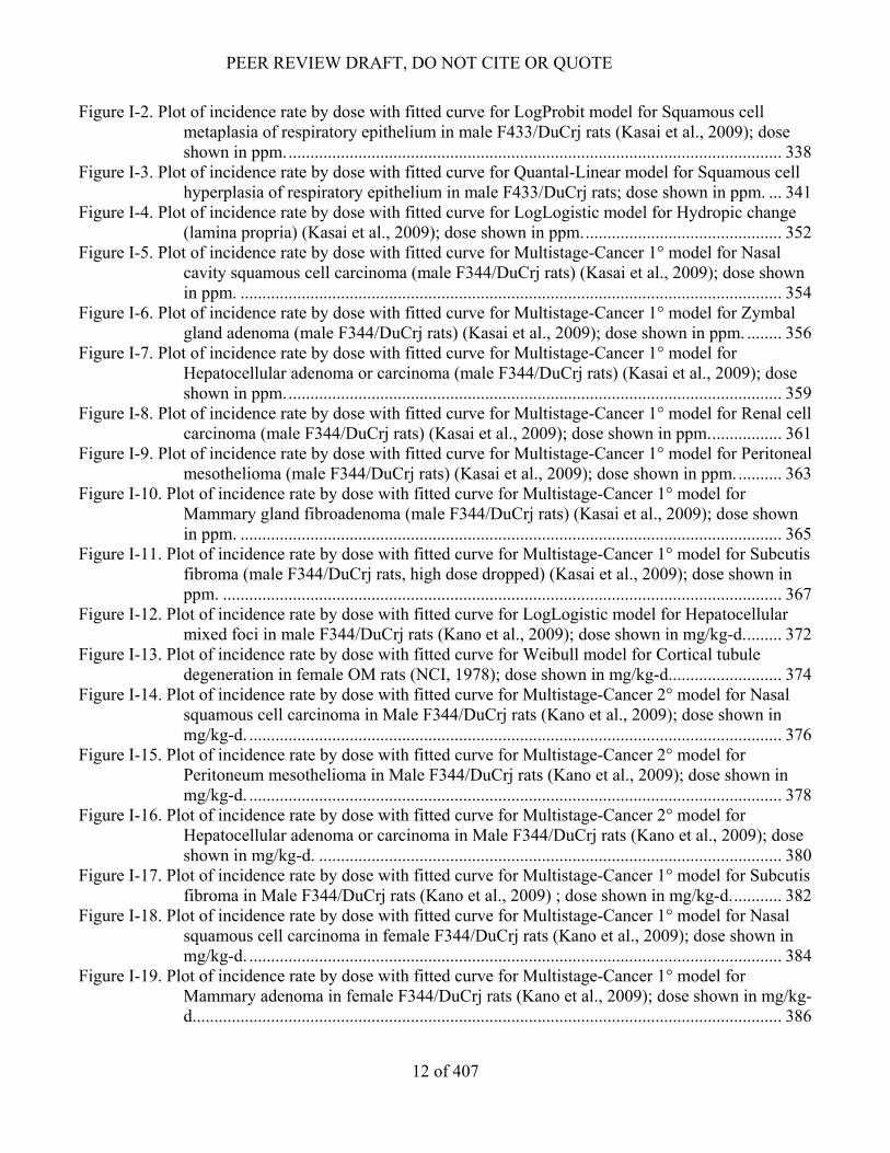
Figure I-2. Plot of incidence rate by dose with fitted curve for LogProbit model for Squamous cell metaplasia of respiratory epithelium in male F433/DuCrj rats (Kasai et al., 2009); dose shown in ppm. ................................................................................................................. 338
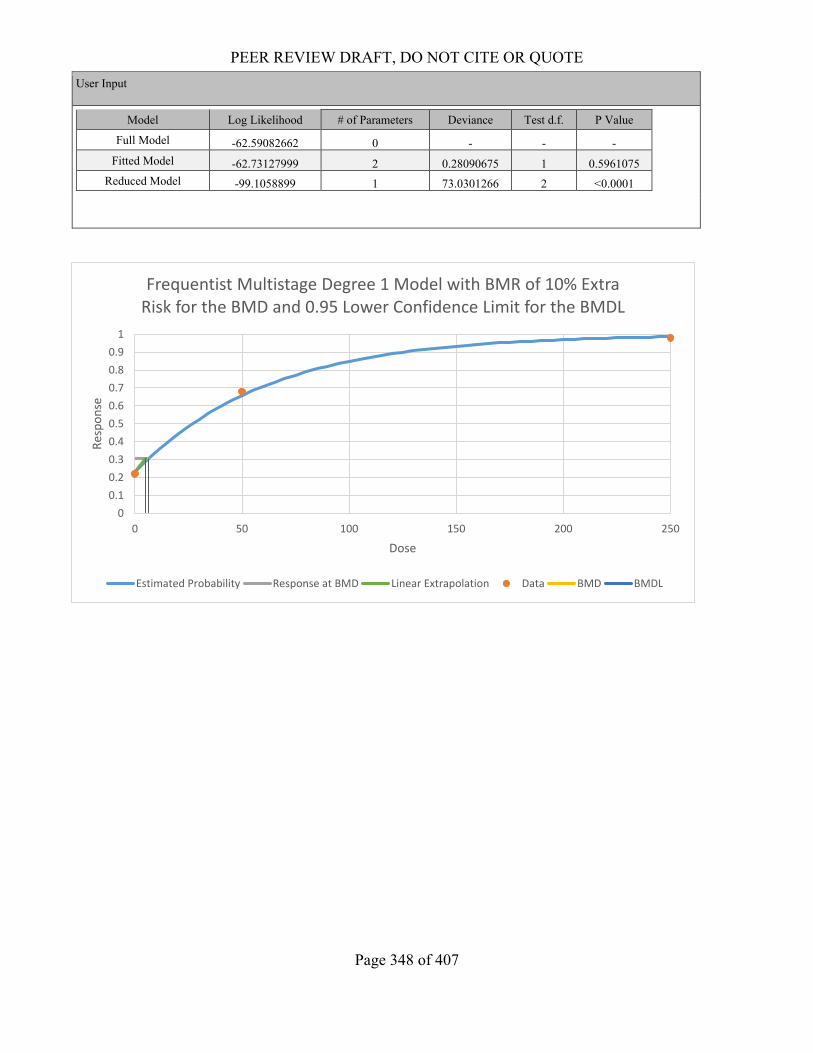
Figure I-3. Plot of incidence rate by dose with fitted curve for Quantal-Linear model for Squamous cell hyperplasia of respiratory epithelium in male F433/DuCrj rats; dose shown in ppm. ... 341
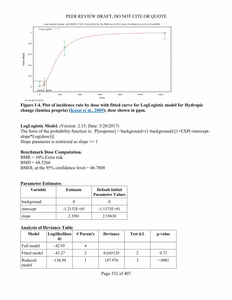
Figure I-4. Plot of incidence rate by dose with fitted curve for LogLogistic model for Hydropic change (lamina propria) (Kasai et al., 2009); dose shown in ppm. ............................................. 352
Figure I-5. Plot of incidence rate by dose with fitted curve for Multistage-Cancer 1° model for Nasal cavity squamous cell carcinoma (male F344/DuCrj rats) (Kasai et al., 2009); dose shown in ppm. ............................................................................................................................ 354
Figure I-6. Plot of incidence rate by dose with fitted curve for Multistage-Cancer 1° model for Zymbal gland adenoma (male F344/DuCrj rats) (Kasai et al., 2009); dose shown in ppm. ........ 356
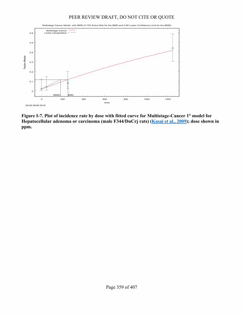
Figure I-7. Plot of incidence rate by dose with fitted curve for Multistage-Cancer 1° model for Hepatocellular adenoma or carcinoma (male F344/DuCrj rats) (Kasai et al., 2009); dose shown in ppm. ................................................................................................................. 359
Figure I-8. Plot of incidence rate by dose with fitted curve for Multistage-Cancer 1° model for Renal cell carcinoma (male F344/DuCrj rats) (Kasai et al., 2009); dose shown in ppm. ................ 361
Figure I-9. Plot of incidence rate by dose with fitted curve for Multistage-Cancer 1° model for Peritoneal mesothelioma (male F344/DuCrj rats) (Kasai et al., 2009); dose shown in ppm. .......... 363
Figure I-10. Plot of incidence rate by dose with fitted curve for Multistage-Cancer 1° model for Mammary gland fibroadenoma (male F344/DuCrj rats) (Kasai et al., 2009); dose shown in ppm. ............................................................................................................................ 365
Figure I-11. Plot of incidence rate by dose with fitted curve for Multistage-Cancer 1° model for Subcutis fibroma (male F344/DuCrj rats, high dose dropped) (Kasai et al., 2009); dose shown in ppm. ................................................................................................................................ 367
Figure I-12. Plot of incidence rate by dose with fitted curve for LogLogistic model for Hepatocellular mixed foci in male F344/DuCrj rats (Kano et al., 2009); dose shown in mg/kg-d. ........ 372
Figure I-13. Plot of incidence rate by dose with fitted curve for Weibull model for Cortical tubule degeneration in female OM rats (NCI, 1978); dose shown in mg/kg-d. ......................... 374
Figure I-14. Plot of incidence rate by dose with fitted curve for Multistage-Cancer 2° model for Nasal squamous cell carcinoma in Male F344/DuCrj rats (Kano et al., 2009); dose shown in mg/kg-d. .......................................................................................................................... 376
Figure I-15. Plot of incidence rate by dose with fitted curve for Multistage-Cancer 2° model for Peritoneum mesothelioma in Male F344/DuCrj rats (Kano et al., 2009); dose shown in mg/kg-d. .......................................................................................................................... 378
Figure I-16. Plot of incidence rate by dose with fitted curve for Multistage-Cancer 2° model for Hepatocellular adenoma or carcinoma in Male F344/DuCrj rats (Kano et al., 2009); dose shown in mg/kg-d. .......................................................................................................... 380
Figure I-17. Plot of incidence rate by dose with fitted curve for Multistage-Cancer 1° model for Subcutis fibroma in Male F344/DuCrj rats (Kano et al., 2009) ; dose shown in mg/kg-d. ........... 382
Figure I-18. Plot of incidence rate by dose with fitted curve for Multistage-Cancer 1° model for Nasal squamous cell carcinoma in female F344/DuCrj rats (Kano et al., 2009); dose shown in mg/kg-d. .......................................................................................................................... 384
Figure I-19. Plot of incidence rate by dose with fitted curve for Multistage-Cancer 1° model for Mammary adenoma in female F344/DuCrj rats (Kano et al., 2009); dose shown in mg/kg-d....................................................................................................................................... 386
PEER REVIEW DRAFT, DO NOT CITE OR QUOTE
13 of 407
Figure I-20. Plot of incidence rate by dose with fitted curve for Multistage-Cancer 2° model for Hepatocellular adenomas or carcinomas female F344/DuCrj rats (Kano et al., 2009); dose shown in mg/kg-d. .......................................................................................................... 388
Figure I-21. Plot of incidence rate by dose with fitted curve for Multistage-Cancer 1° model for Hepatocellular adenomas or carcinomas in male CrjBDF1 mice (Kano et al., 2009); dose shown in mg/kg-d. .......................................................................................................... 390
Figure I-22. Plot of incidence rate by dose with fitted curve for Multistage-Cancer 2° model for Nasal cavity tumors in Sherman rats (Kociba et al., 1974); dose shown in mg/kg-d. .............. 392
Figure I-23. Plot of incidence rate by dose with fitted curve for Multistage-Cancer 1° model for Liver tumors in Sherman rats (male and female combined) (Kociba et al., 1974); dose shown in mg/kg-d. .......................................................................................................................... 394
Figure I-24. Plot of incidence rate by dose with fitted curve for Multistage-Cancer 1° model for Nasal squamous cell carcinomas in female OM rats (MS models) (NCI, 1978); dose shown in mg/kg-d. .......................................................................................................................... 396
Figure I-25. Plot of incidence rate by dose with fitted curve for Multistage-Cancer 1° model for Hepatocellular adenoma in female OM rats (NCI, 1978); dose shown in mg/kg-d. ...... 398
Figure I-26. Plot of incidence rate by dose with fitted curve for Multistage-Cancer 1° model for Hepatocellular adenomas or carcinomas in male B6C3F1 mice (NCI, 1978); dose shown in mg/kg-d. ...................................................................................................................... 400
Figure I-27. Plot of incidence rate by dose with fitted curve for Multistage-Cancer 1° model for Hepatocellular adenomas or carcinomas in female B6C3F1 mice (NCI, 1978); dose shown in mg/kg-d. .......................................................................................................... 402
PEER REVIEW DRAFT, DO NOT CITE OR QUOTE
14 of 407
ACKNOWLEDGEMENTS This report was developed by the United States Environmental Protection Agency (U.S. EPA), Office of Chemical Safety and Pollution Prevention (OCSPP), Office of Pollution Prevention and Toxics (OPPT) with support from the Office of Research and Development (ORD). Acknowledgements The OPPT Assessment Team gratefully acknowledges participation and/or input from Intra-agency reviewers that included multiple offices within EPA, Inter-agency reviewers that included multiple Federal agencies, and assistance from EPA contractors GDIT (Contract No. CIO-SP3, HHSN316201200013W), ERG (Contract No. EP-W-12-006), Versar (Contract No. EP-W-17-006), ICF (Contract No. EPC14001) and SRC (Contract No. EP-W-12-003). Docket Supporting information can be found in public docket: EPA-HQ-OPPT-2016-0723. Disclaimer Reference herein to any specific commercial products, process or service by trade name, trademark, manufacturer or otherwise does not constitute or imply its endorsement, recommendation or favoring by the United States Government.
ABBREVIATIONS ACC American Chemistry Council °C Degrees Celsius atm atmosphere(s) AEC Acute Exposure Concentration AES Alkyl Ethoxysulphates AQS Air Quality System ATSDR Agency for Toxic Substances and Disease Registries BLS Bureau of Labor Statistics CAA Clean Air Act CASRN Chemical Abstract Service Registry Number CBI Confidential Business Information CCL Candidate Contaminant List CDR Chemical Data Reporting CNS Central Nervous System CSF Cancer Slope Factor DHHS Department of Health and Human Services DMR Discharge Munitions Report EC European Commission ECHA European Chemicals Agency E-FAST Exposure and Fate Assessment Screening Tool EPA Environmental Protection Agency ESD Emission Scenario Document EU European Union EUSES European Union System for the Evaluation of Substances FDA Food and Drug Administration HEAA β-Hydroxyethoxy Acetic Acid HAP Hazardous Air Pollutant Hg Mercury HPV High Production Volume IARC International Agency for Research on Cancer ICSC International Chemical Safety Cards ILO International Labor Organization IRIS Integrated Risk Information System IUR Inventory Update Reporting Rule; or Inhalation Unit Risk kg Kilogram(s) KOW Octanol:Water Partition Coefficient LADC Lifetime Average Daily Concentration lb Pound LOAEC Lowest Observed Adverse Effect Concentration LOAEL Lowest Observed Adverse Effect Level Log KOW Logarithmic Octanol:Water Partition Coefficient MATC Maximum Acceptable Toxicant Concentration mg Milligram(s) µg Microgram(s) MOE Margin of Exposure MRL Minimal Risk Level
PEER REVIEW DRAFT, DO NOT CITE OR QUOTE
16 of 407
NAICS North American industrial Classification System NAS National Academies of Science NATA National Air-Toxics Assessment NEI National Emissions Inventory NIOSH National Institute of Occupational Safety and Health NOEC No Observed Effect Concentration NOAEL No Observed Adverse Effect Level NPL National Priorities List NTP National Toxicology Program OAR Office of Air and Radiation OCF One Component Foam OCSPP Office of Chemical Safety and Pollution Prevention OECD Organisation for Economic Co-operation and Development OES Occupational Exposure Scenario OLEM Office of Land and Emergency Management ONU Occupational non-user OPPT Office of Pollution Prevention and Toxics OSHA Occupational Safety and Health Administration OSWER Office of Solid Waste and Emergency Response OW Office of Water PBPK Physiologically Based Pharmacokinetic PBT Persistent, Bioaccumulative, Toxic PBZ Personal Breathing Zone PDE Permitted Daily Exposure PEC Predicted Environmental Concentration PEL Permissible Exposure Level PFIA Problem Formulation and Initial Assessment POD Point of Departure ppb Parts per Billion ppm Parts per Million PV Production Volume PWS Public Water System RA Risk Assessment RAR Risk Assessment Report REACH Registration, Evaluation, Authorisation and Restriction of Chemicals REL Recommended Exposure Level RfC Reference Concentration RfD Reference Dose SDS Safety Data Sheet SPFs Spray Polyurethane Foams SUSB Statistics of US Businesses TCA 1,1,1-Trichloroethane TIAC Time Integrated Air Concentration TLV Threshold Limit Value TRI Toxic Release Inventory TSCA Toxic Substances Control Act TWA Time Weighted Average
PEER REVIEW DRAFT, DO NOT CITE OR QUOTE
17 of 407
UCMR Unregulated Contaminant Monitoring Rule US United States VCCEP Voluntary Children’s Chemical Evaluation Program WHO World Health Organisation WWTP Wastewater Treatment Plant Yr Year
PEER REVIEW DRAFT, DO NOT CITE OR QUOTE
18 of 407
1 EXECUTIVE SUMMARY This draft risk evaluation for 1,4-dioxane was performed in accordance with the Frank R. Lautenberg Chemical Safety for the 21st Century Act and is being disseminated for public comment and peer review. The Frank R. Lautenberg Chemical Safety for the 21st Century Act amended the Toxic Substances Control Act, the Nation’s primary chemicals management law, in June 2016. As per EPA’s final rule, Procedures for Chemical Risk Evaluation Under the Amended Toxic Substances Control Act (82 FR 33726), EPA is taking comment on this draft, and will also obtain peer review on this draft risk evaluation for 1,4-dioxane. All conclusions, findings, and determinations in this document are preliminary and subject to comment. The final risk evaluation may change in response to public comments received on the draft risk evaluation and/or in response to peer review, which itself may be informed by public comments. TSCA § 26(h) and (i) require EPA to use scientific information, technical procedures, measures, methods, protocols, methodologies and models consistent with the best available science and to base its decisions on the weight of the scientific evidence. To meet these TSCA § 26 science standards, EPA used the TSCA systematic review process described in the Application of Systematic Review in TSCA Risk Evaluations document (U.S. EPA, 2018b). The process complements the risk evaluation process in that the data collection, data evaluation and data integration stages of the systematic review process are used to develop the exposure, fate and hazard assessments for risk evaluations. 1,4-Dioxane is a clear volatile liquid used primarily as a solvent and is subject to federal and state regulations and reporting requirements. 1,4-Dioxane has been reportable to Toxics Release Inventory (TRI) chemical under Section 313 of the Emergency Planning and Community Right-to-Know Act (EPCRA) since 1987. It is designated a Hazardous Air Pollutant (HAP) under the Clean Air Act (CAA), and is a hazardous substance under the Comprehensive Environmental Response, Compensation and Liability Act (CERCLA). It was listed on the Safe Drinking Water (SDWA) Candidate Contaminant List (CCL) and identified in the third Unregulated Contaminant Monitoring Rule (UCMR3). 1,4-Dioxane is currently manufactured, processed, distributed, and disposed of following use in industrial processes with industrial and commercial conditions of use. Manufacturing sites produce 1,4-dioxane in liquid form at concentrations greater or equal to 90% [EPA-HQ-OPPT-2016-0723-0012; (BASF, 2017)] and 1,4-dioxane is also imported. EPA evaluated the following conditions of use: manufacturing; processing; functional fluids in open and closed systems; laboratory chemicals; adhesives and sealants (professional film cement); spray polyurethane foam; printing and printing compositions; disposal of waste materials containing 1,4-dioxane; and dry film lubricant. The total aggregate production volume is approximately 1 million pounds. Approach EPA used reasonably available information, defined in 40 CFR 702.33 as information that EPA possesses, or can reasonably obtain and synthesize for use in risk evaluations, considering the deadlines for completing the evaluation, in a fit-for-purpose approach, to develop a risk evaluation that relies on the best available science and is based on the weight of the scientific evidence. EPA used previous analyses as a starting point for identifying key and supporting studies to inform the exposure, fate and hazard assessments. EPA also evaluated other studies that were published since these reviews. EPA reviewed the information and evaluated the quality of the methods and reporting of results of the
individual studies using the evaluation strategies described in Application of Systematic Review in TSCA Risk Evaluations (U.S. EPA, 2018b). In the problem formulation, EPA identified the conditions of use and presented two conceptual models and an analysis plan for this draft risk evaluation. In this draft risk evaluation, EPA evaluated the risk to workers and occupational non-users (ONUs) from inhalation and dermal exposures by comparing the estimated occupational exposures to acute and chronic human health hazards. ONUs are workers at the facility who neither directly perform activities near the 1,4-dioxane source area nor regularly handle 1,4-dioxane. The job classifications for ONUs could be dependent on the conditions of use. EPA utilized environmental fate parameters and physical-chemical properties, and modelling, to assess ambient water exposure to aquatic organisms, sediments and land-applied biosolids. While 1,4-dioxane is present in various environmental media such as groundwater, surface water, and air, EPA determined during problem formulation that no further analysis beyond what was presented in the problem formulation document would be done for those environmental exposure pathways in this draft risk evaluation. However, risk determinations were not made as part of problem formulation; therefore, the results from these analyses are presented in this draft risk evaluation and used to inform the risk determination section. The exposure and environmental hazard analyses for the environmental release pathways for ambient water exposure to aquatic organisms, sediments, and land-applied biosolids conducted based on a qualitative assessment of the physical-chemical properties and fate of 1,4-dioxane in the environment and a quantitative comparison of hazards and exposures for aquatic organisms are presented in sections 3.1, 3.3 and 5.1. EPA evaluated acute and chronic inhalation exposures to workers and ONUs in association with 1,4-dioxane for the conditions of use identified. EPA used inhalation monitoring data that was from literature sources where reasonably available and that met data evaluation criteria and modeling approaches to estimate potential inhalation exposures. EPA also estimated dermal doses for workers in these scenarios since dermal monitoring data was not reasonably available. These analyses are described in section 3.4 of this draft risk evaluation. In the human health hazards section, EPA evaluated reasonably available information and identified hazard endpoints including acute/chronic toxicity, non-cancer effects, and cancer for inhalation and dermal exposure for relevant chronic exposures. EPA used an approach based on the Framework for Human Health Risk Assessment to Inform Decision Making (U.S. EPA, 2014d) to evaluate, extract and integrate 1,4-dioxane’s human health hazard and dose-response information. EPA reviewed key and supporting information from previous hazard assessments [EPA IRIS Assessments (U.S. EPA, 2013c, 2010), an ATSDR Toxicological Profile (ATSDR, 2012), a Canadian Screening Assessment (Health Canada, 2010), a European Union (EU) Risk Assessment Report (ECJRC, 2002), and an Interim AEGL (U.S. EPA, 2005b)]. EPA also screened and evaluated new studies that were published since these reviews (i.e. from 2013 – 2018). EPA developed a hazard and dose-response analysis for inhalation and oral hazard endpoints identified based on the weight of the scientific evidence considering EPA, National Research Council (NRC), and European Chemicals Agency (ECHA) risk assessment guidance and selected the points of departure (POD) for acute/chronic, non-cancer endpoints, and inhalation unit risk and cancer slope factors for cancer risk estimates. Potential health effects of 1,4-dioxane exposure described in the literature include effects on the liver, kidneys, respiratory system, neurological endpoints, and cancer. EPA identified
acute PODs for inhalation and dermal exposures based on acute liver toxicity observed in rats (Mattie et al., 2012). The chronic POD for inhalation exposures are based on effects on nasal tissue in rats (Kasai et al., 2009). EPA provided chronic PODs for dermal exposure that extrapolated from effects on liver following exposure through inhalation (Mattie et al., 2012) and exposure through drinking water (Kano et al., 2009; NCI, 1978; Kociba et al., 1974). EPA also considered the current evidence for two potential modes of action that would support either a threshold approach or a linear non-threshold approach for estimating cancer risk. The risk evaluation ultimately calculated cancer risk with a linear model using cancer slope factors based on evidence of increased risk of cancer in rats exposed to 1,4-dioxane through air or drinking water (Kano et al., 2009; Kasai et al., 2009). The results of these analyses are described in section 4.2. Uncertainties: 1,4-Dioxane is a multi-site carcinogen and may have more than one MOA. There was a high degree of uncertainty in each of the MOA hypotheses considered in this evaluation (e.g., mutagenic mode of action or threshold response to cytotoxicity and regenerative hyperplasia for liver tumors). Chronic non-cancer risk estimates from inhalation exposures were based on portal of entry effects in the respiratory tract. These effects are relevant to inhalation exposures and are more sensitive than the observed systemic effects. Dermal extrapolation and dermal absorption were also sources of uncertainty in the dermal risk assessment for both dermal cancer and noncancer estimates of risk. Inhalation to dermal and oral to dermal route-to-route extrapolations were compared for relevance to dermal exposures. Metabolism occurs in both oral and dermal routes and portal of entry effects from inhalation are not as relevant to dermal exposures. Risk Characterization For environmental risk, EPA estimated risks based on a qualitative assessment of the physical-chemical properties and fate of 1,4-dioxane in the environment for sediment and land-applied biosolids, and a quantitative comparison of hazards and exposures for aquatic organisms. EPA utilized a risk quotient (RQ) to compare the environmental concentration to the effect level to characterize the risk to aquatic organisms. Table 5-2 in this draft risk evaluation summarizes the RQs for acute and chronic risks of 1,4-dioxane for aquatic organisms. EPA included a qualitive assessment describing 1,4-dioxane exposure in sediments and land-applied biosolids.1,4-Dioxane is not expected to accumulate in sediments and is expected to be mobile in soil and to migrate to water or volatilize to air. The results of the risk characterization are in section 5.1. EPA used a Margin of Exposure (MOE) approach to identify potential non-cancer human health risks and allow for a range of risk estimates. EPA estimated potential inhalation cancer risk from chronic exposures to 1,4-dioxane by using a range of inhalation unit risk values multiplied by the chronic exposure to workers and ONUs for each COU. For dermal cancer risk, EPA used the cancer slope factor multiplied by the chronic exposure to workers and ONUs for each COU. In section 5.2, EPA presents 8 tables which describe risk estimates: for acute/short-term and chronic exposures via inhalation (non-cancer) to workers and ONUs; chronic exposures via inhalation (cancer) to workers and ONUs; and acute and chronic dermal exposure (non-cancer) and chronic dermal exposure (cancer) to workers. The results of these analyses are presented in section 5.2.
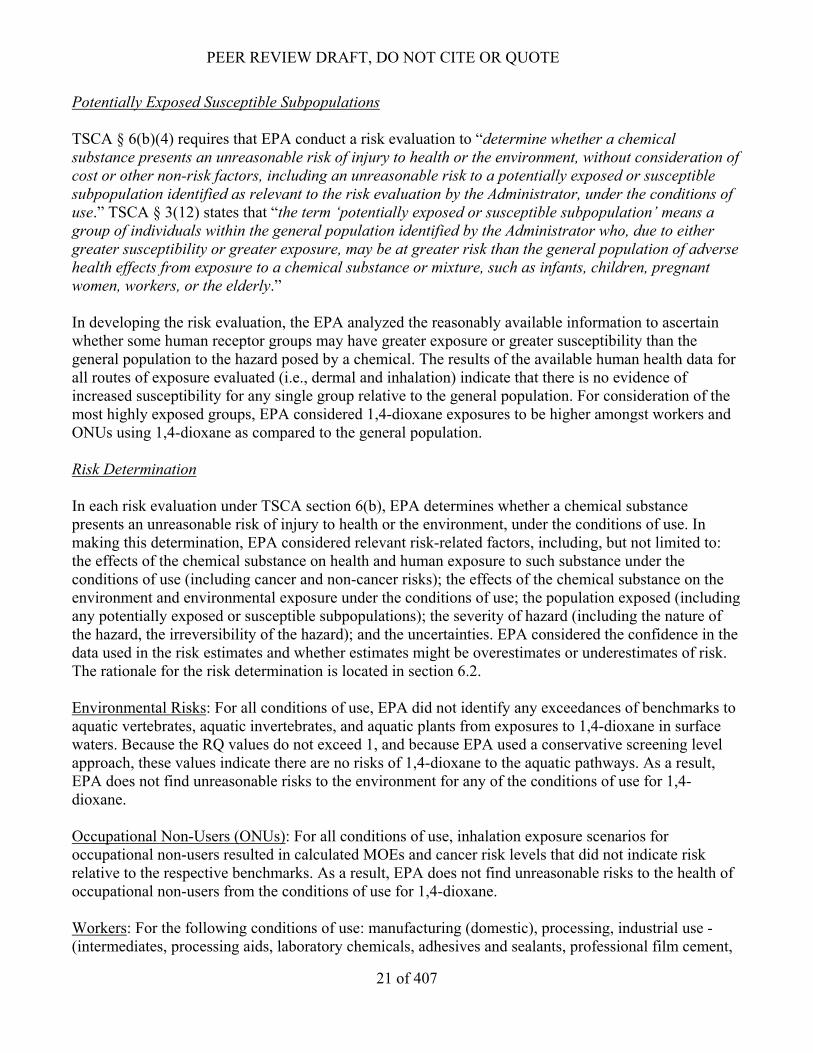
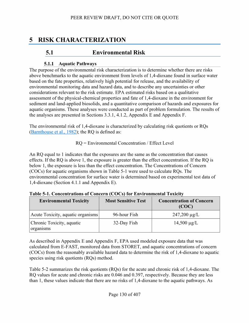
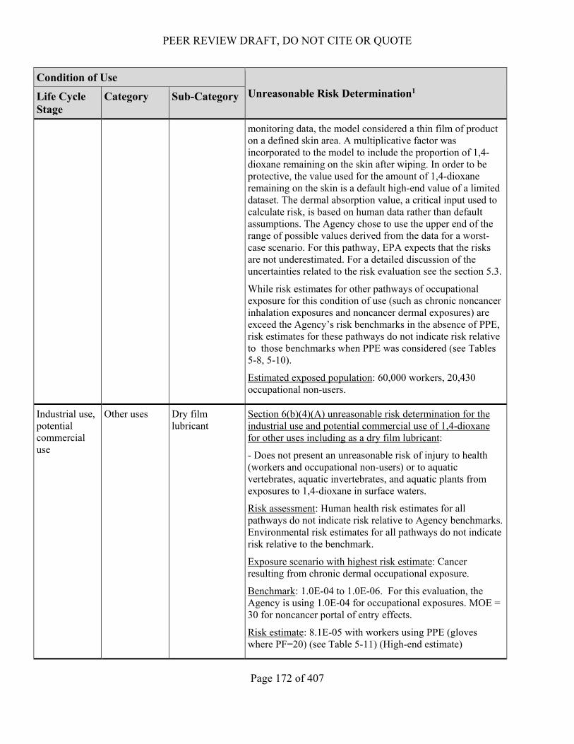
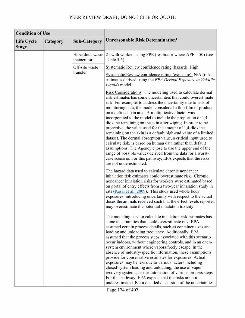
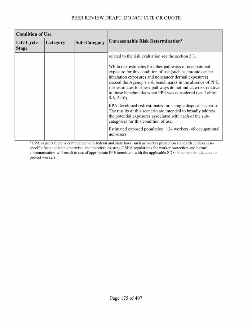
Potentially Exposed Susceptible Subpopulations TSCA § 6(b)(4) requires that EPA conduct a risk evaluation to “determine whether a chemical substance presents an unreasonable risk of injury to health or the environment, without consideration of cost or other non-risk factors, including an unreasonable risk to a potentially exposed or susceptible subpopulation identified as relevant to the risk evaluation by the Administrator, under the conditions of use.” TSCA § 3(12) states that “the term ‘potentially exposed or susceptible subpopulation’ means a group of individuals within the general population identified by the Administrator who, due to either greater susceptibility or greater exposure, may be at greater risk than the general population of adverse health effects from exposure to a chemical substance or mixture, such as infants, children, pregnant women, workers, or the elderly.” In developing the risk evaluation, the EPA analyzed the reasonably available information to ascertain whether some human receptor groups may have greater exposure or greater susceptibility than the general population to the hazard posed by a chemical. The results of the available human health data for all routes of exposure evaluated (i.e., dermal and inhalation) indicate that there is no evidence of increased susceptibility for any single group relative to the general population. For consideration of the most highly exposed groups, EPA considered 1,4-dioxane exposures to be higher amongst workers and ONUs using 1,4-dioxane as compared to the general population. Risk Determination In each risk evaluation under TSCA section 6(b), EPA determines whether a chemical substance presents an unreasonable risk of injury to health or the environment, under the conditions of use. In making this determination, EPA considered relevant risk-related factors, including, but not limited to: the effects of the chemical substance on health and human exposure to such substance under the conditions of use (including cancer and non-cancer risks); the effects of the chemical substance on the environment and environmental exposure under the conditions of use; the population exposed (including any potentially exposed or susceptible subpopulations); the severity of hazard (including the nature of the hazard, the irreversibility of the hazard); and the uncertainties. EPA considered the confidence in the data used in the risk estimates and whether estimates might be overestimates or underestimates of risk. The rationale for the risk determination is located in section 6.2. Environmental Risks: For all conditions of use, EPA did not identify any exceedances of benchmarks to aquatic vertebrates, aquatic invertebrates, and aquatic plants from exposures to 1,4-dioxane in surface waters. Because the RQ values do not exceed 1, and because EPA used a conservative screening level approach, these values indicate there are no risks of 1,4-dioxane to the aquatic pathways. As a result, EPA does not find unreasonable risks to the environment for any of the conditions of use for 1,4-dioxane. Occupational Non-Users (ONUs): For all conditions of use, inhalation exposure scenarios for occupational non-users resulted in calculated MOEs and cancer risk levels that did not indicate risk relative to the respective benchmarks. As a result, EPA does not find unreasonable risks to the health of occupational non-users from the conditions of use for 1,4-dioxane. Workers: For the following conditions of use: manufacturing (domestic), processing, industrial use - (intermediates, processing aids, laboratory chemicals, adhesives and sealants, professional film cement,
PEER REVIEW DRAFT, DO NOT CITE OR QUOTE
22 of 407
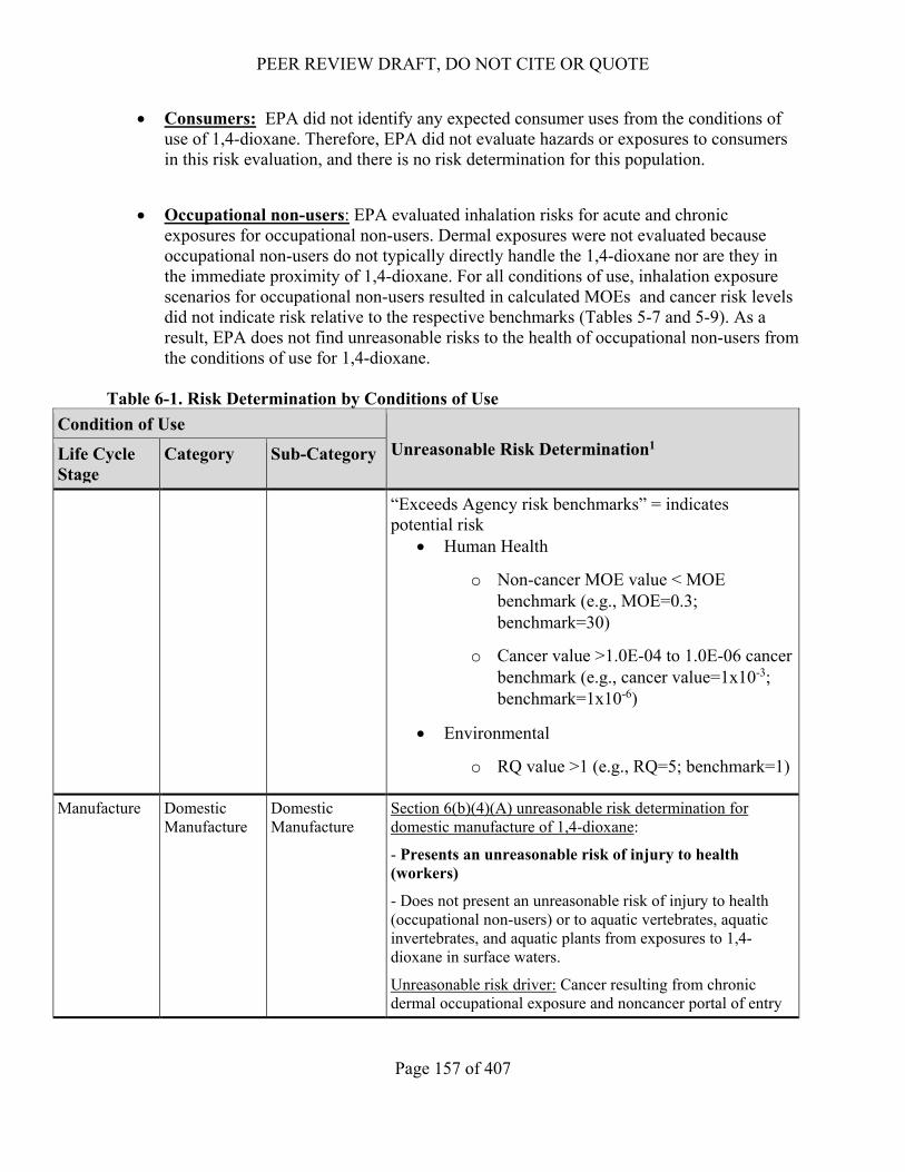
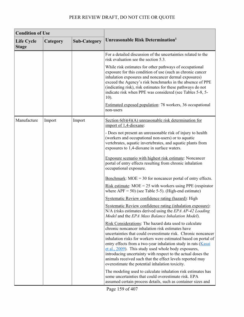
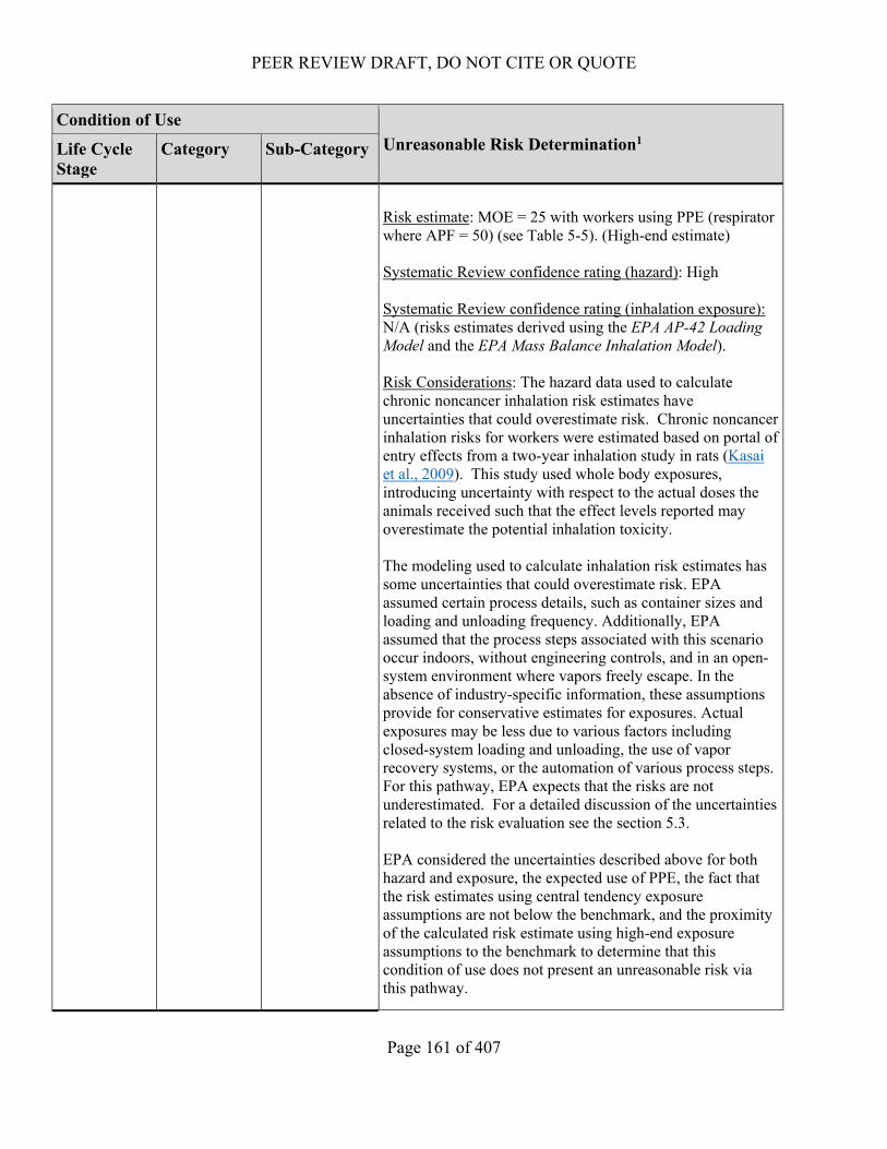
printing and printing compositions), and disposal, EPA assessed inhalation and/or dermal exposure scenarios that resulted in MOEs and/or cancer risk estimates that indicate risks relevant to the respective benchmarks. EPA considered those risk estimates; confidence in the data used in the risk estimates and uncertainties associated with the risk estimates; and relevant risk-related factors described above and has preliminarily concluded that the aforementioned conditions of use present an unreasonable risk of injury to health, as set forth in the risk determination section of this draft risk evaluation. This draft document’s preliminarily determination of unreasonable risk does not mean that this is EPA’s final conclusion. EPA will consider further input through scientific and public review. For the following conditions of use: manufacturing (import), processing (repackaging), distribution, and industrial use (functional fluids in open and closed systems, spray polyurethane foam, dry film lubricant), EPA assessed inhalation and/or dermal exposure scenarios that resulted in MOEs and/or cancer risk estimates that do not indicate risk relevant to the respective benchmarks. As a result, EPA finds that the aforementioned conditions of use do not present an unreasonable risk of injury to health.
2 INTRODUCTION This document presents for comment the draft risk evaluation for 1,4-dioxane under the Frank R. Lautenberg Chemical Safety for the 21st Century Act. The Frank R. Lautenberg Chemical Safety for the 21st Century Act amended the Toxic Substances Control Act, the Nation’s primary chemicals management law, in June 2016. The Agency published the Scope of the Risk Evaluation for 1,4-dioxane (U.S. EPA, 2017d) in June 2017, and the problem formulation in June, 2018 (U.S. EPA, 2018c), which represented the analytical phase of risk evaluation in which “the purpose for the assessment is articulated, the problem is defined, and a plan for analyzing and characterizing risk is determined” as described in Section 2.2 of the Framework for Human Health Risk Assessment to Inform Decision Making. The EPA received comments on the published problem formulation for 1,4-dioxane and has considered the comments specific to 1,4-dioxane, as well as more general comments regarding the EPA’s chemical risk evaluation approach for developing the draft risk evaluations for the first 10 chemicals the EPA is evaluating. The problem formulation identified the conditions of use and presented two conceptual models and an analysis plan. In this risk evaluation, EPA evaluated the risk to workers from inhalation and dermal exposures by comparing the estimated occupational exposures to acute and chronic human health hazards. While 1,4-dioxane is present in various environmental media such as groundwater, surface water, and air, EPA determined during problem formulation that no further analysis of the environmental release pathways for ambient water exposure to aquatic organisms, sediments, and land-applied biosolids needed to be conducted based on a qualitative assessment of the physical chemical properties and fate of 1,4-dioxane in the environment and a quantitative comparison of hazards and exposures for aquatic organisms. Risk determinations were not made as part of problem formulation; therefore, the results from these analyses are presented in this risk evaluation and used to inform the risk determination section of this draft risk evaluation. EPA used reasonably available information consistent with best available science for physical and chemical properties, environmental fate properties, occupational exposure, environmental hazard, and human health hazard studies according to the systematic review process. For human exposure pathways,
EPA evaluated inhalation exposures to vapors and mists for workers and occupational non-users and dermal exposures for skin contact with liquids for workers. For environmental release pathways, EPA characterized risks to ecological receptors from surface water, sediment, and land-applied biosolids in the risk characterization section of this draft risk evaluation based on the analyses presented in the problem formulation. The document is structured such that Introduction, Section 2, presents the basic physical-chemical properties of 1,4-dioxane, as well as a background on uses, regulatory history, conditions of use and conceptual models, with emphasis on any changes since the publication of the problem formulation. This section also includes a discussion of the systematic review process utilized in this draft risk evaluation. Exposures, Section 3, provides a discussion and analysis of the exposures, both human and environmental that can be expected based on the conditions of use for 1,4-dioxane. Hazards, Section 4, discusses environmental and human health hazards of 1,4-dioxane. Risk characterization is in Section 5, which integrates and assesses reasonably available information on human health and environmental hazards and exposures, as required by TSCA (15 U.S.C 2605(b)(4)(F)). This section also includes a discussion of any uncertainties and how they impact the risk evaluation. In Risk Determination, Section 5.4, the agency presents the determination of whether risk posed by the chemical substance is unreasonable as required under TSCA 15 U.S.C. 2605(b)(4). As per EPA’s final rule, Procedures for Chemical Risk Evaluation Under the Amended Toxic Substances Control Act (82 FR 33726), this draft risk evaluation is subject to both public comment and peer review, which are distinct but related processes. EPA is providing 60 days for public comment on this draft risk evaluation during the peer review meeting to inform the EPA Science Advisory Committee on Chemicals (SACC) peer review process. The EPA seeks public comment on all aspects of this draft risk evaluation. This is also an opportunity for the EPA to receive any additional information that might be relevant to the science underlying the risk evaluation and the outcome of the systematic review associated with 1,4-dioxane. This satisfies TSCA (15 U.S.C 2605(4)(H)), which requires the EPA to provide public notice and an opportunity for comment on a draft risk evaluation prior to publishing a final risk evaluation. Peer review will be conducted in accordance with EPA's regulatory procedures for chemical risk evaluations, including using the EPA Peer Review Handbook and other methods consistent with section 26 of TSCA (See 40 CFR § 702.45). As explained in the Risk Evaluation Rule, the purpose of peer review is for the independent review of the science underlying the risk assessment. Peer review will therefore address aspects of the underlying science as outlined in the charge to the peer review panel such as hazard assessment, assessment of dose-response, exposure assessment, and risk characterization. Peer-review supports scientific rigor and enhances transparency in the risk evaluation process. As the EPA explained in the Risk Evaluation Rule, it is important for peer reviewers to consider how the underlying risk evaluation analyses fit together to produce an integrated risk characterization, which will form the basis of an unreasonable risk determination. The EPA believes peer reviewers will be most effective in this role if they receive the benefit of public comments on draft risk evaluations prior to peer review. For this reason, EPA is providing the opportunity for public comment before peer review on this draft risk evaluation. The final risk evaluation may change in response to public comments received on the draft risk evaluation and/or in response to peer review, which itself may be informed by public
comments. The EPA will respond to public and peer review comments received on the draft risk evaluation when it issues the final risk evaluation. EPA solicited input on the first 10 chemicals, including 1,4-dioxane, as it developed use dossiers, scope documents, and problem formulations. At each step, EPA received information and comments specific to individual chemicals and of a more general nature relating to various aspects of the risk evaluation process, technical issues, and the regulatory and statutory requirements. EPA has considered comments and information received at each step in the process and factored in the information and comments as the Agency deemed appropriate and relevant including comments on the published problem formulation of 1,4-dioxane. Thus, in addition to any new comments on the draft risk evaluation, the public should re-submit or clearly identify at this point any previously filed comments, modified as appropriate, that are relevant to this risk evaluation and that the submitter believes have not been addressed. EPA does not intend to further respond to comments submitted prior to the publication of this draft risk evaluation unless they are clearly identified in comments on this draft risk evaluation.
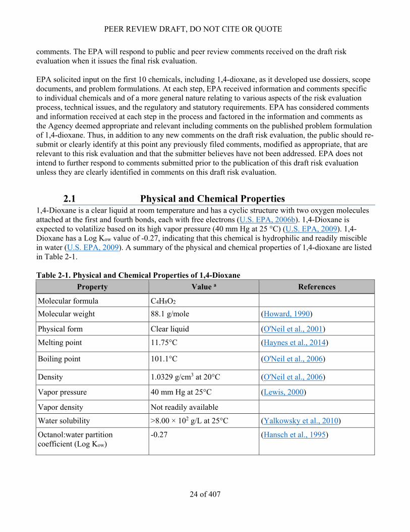
2.1 Physical and Chemical Properties 1,4-Dioxane is a clear liquid at room temperature and has a cyclic structure with two oxygen molecules attached at the first and fourth bonds, each with free electrons (U.S. EPA, 2006b). 1,4-Dioxane is expected to volatilize based on its high vapor pressure (40 mm Hg at 25 °C) (U.S. EPA, 2009). 1,4-Dioxane has a Log Kow value of -0.27, indicating that this chemical is hydrophilic and readily miscible in water (U.S. EPA, 2009). A summary of the physical and chemical properties of 1,4-dioxane are listed in Table 2-1. Table 2-1. Physical and Chemical Properties of 1,4-Dioxane
Property Value a References
Molecular formula C4H8O2 Molecular weight 88.1 g/mole (Howard, 1990)
Physical form Clear liquid (O'Neil et al., 2001)
Melting point 11.75°C (Haynes et al., 2014)
Boiling point 101.1°C (O'Neil et al., 2006)
Density 1.0329 g/cm3 at 20°C (O'Neil et al., 2006)
Vapor pressure 40 mm Hg at 25°C (Lewis, 2000)
Vapor density Not readily available
Water solubility ˃8.00 × 10² g/L at 25°C (Yalkowsky et al., 2010)
Henry’s Law constant 4.8 × 10⁻⁶ atm-m3/mole at 25°C
4.93 × 10⁻⁴ atm-m3/mole at 40°C
(Sander, 2017); (Howard, 1990);(Atkins, 1986)
Flash point 18.3°C (open cup) (Lewis, 2012)
Autoflammability 180 °C at atmospheric pressure (USCG, 1999)
Viscosity 0.0120 cP at 25°C (O'Neil, 2013)
Refractive index 1.4224 at 20°C (Haynes et al., 2014)
Dielectric constant 2.209 Farad per meter (Bruno and PDN, 2006) a Measured unless otherwise noted
2.2 Uses and Production Volume The EPA’s Chemical Data Reporting (CDR) database (U.S. EPA, 2016a) reported that there were two manufacturers producing or importing 1,059,980 pounds of 1,4-dioxane in the U.S. in 2015 (see Table 2-2). The total volume (in lbs.) of 1,4-dioxane manufactured (including imports) in the U.S. from 2012 to 2015 indicates that production has varied over that time. Historically, 90% of 1,4-dioxane production was used as a stabilizer in chlorinated solvents such as 1,1,1-trichloroethane (TCA)(ATSDR, 2012); however, use of 1,4-dioxane has decreased since TCA was phased out by the Montreal Protocol in 1995 (NTP, 2011; ECJRC, 2002). Based on the lack of information on reported uses (Sapphire Group, 2007), EPA concludes that many other industrial, commercial and consumer uses were also stopped., 90% of 1,4-dioxane production was used as a stabilizer in chlorinated solvents such as 1,1,1-trichloroethane (TCA)(ATSDR, 2012); however, use of 1,4-dioxane has decreased since TCA was phased out by the Montreal Protocol in 1995 (NTP, 2011; ECJRC, 2002). Based on the lack of information on reported uses (Sapphire Group, 2007), EPA concludes that many other industrial, commercial and consumer uses were also stopped. Table 2-2. Production Volume of 1,4-Dioxane in Chemical Data Reporting (CDR) Reporting Period (2012 to 2015) a
Reporting Year 2012 2013 2014 2015
Total Aggregate Production Volume (lbs.)
894,505 1,043,627 474,331 1,059,980
a The CDR data for the 2016 reporting period is available via ChemView (https://java.epa.gov/chemview) (U.S. EPA, 2014a). Because of an ongoing CBI substantiation process required by amended TSCA, the CDR data available in the draft risk evaluation document is more specific than currently in ChemView.
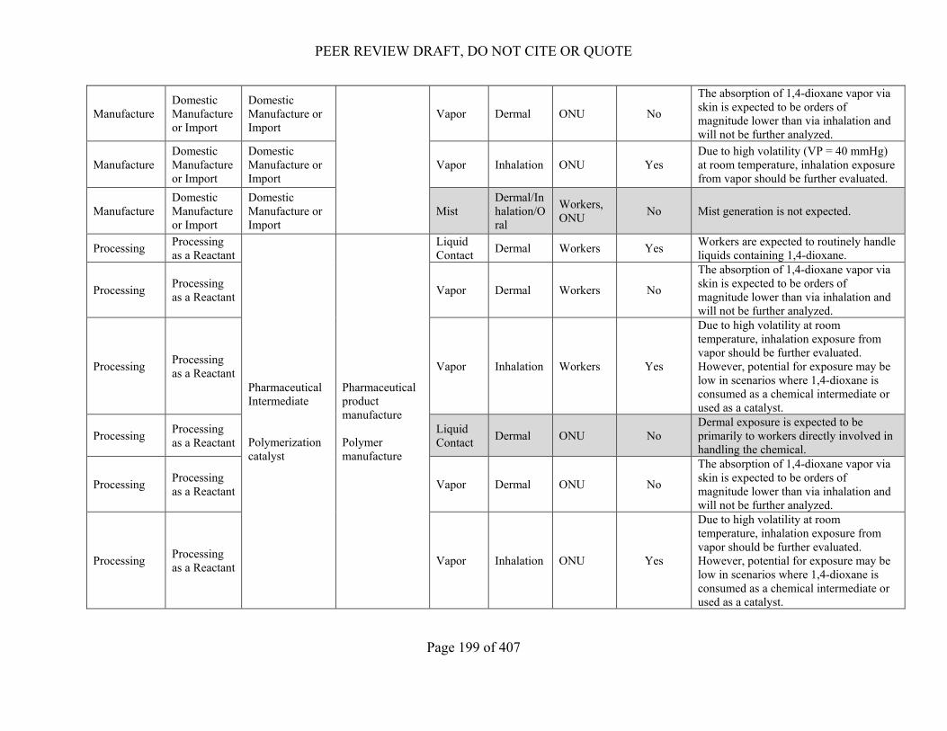
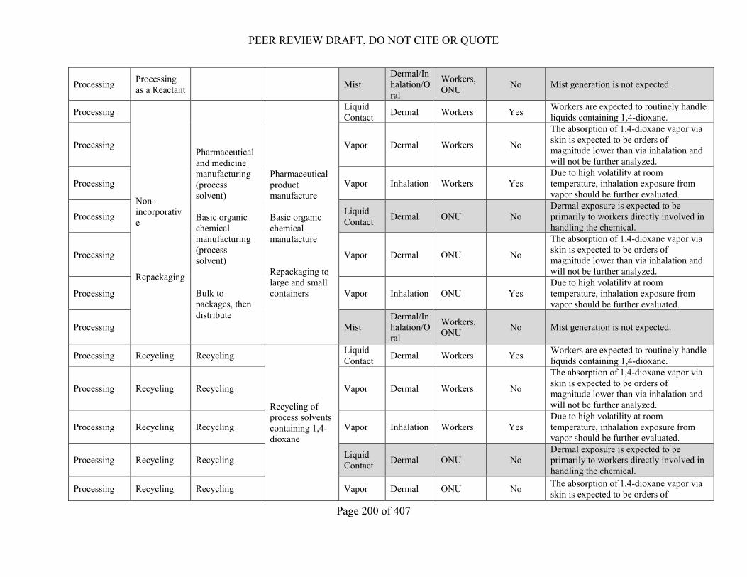
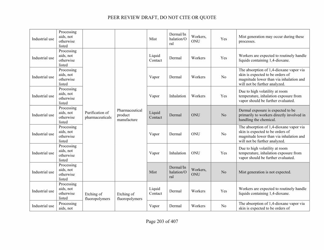
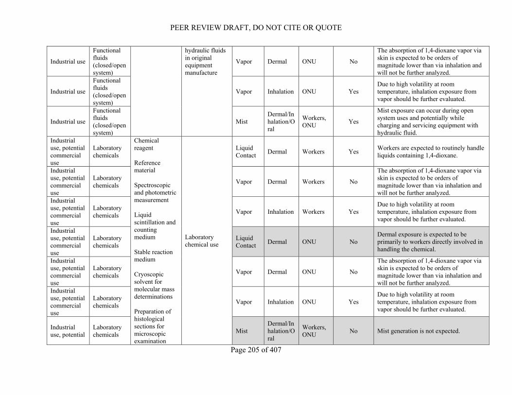
1,4-Dioxane is currently manufactured, processed, distributed and used in industrial processes and for industrial and commercial uses. Manufacturing sites produce 1,4-dioxane in liquid form at concentrations greater or equal to 90% [EPA-HQ-OPPT-2016-0723-0012; (BASF, 2017)] and 1,4-dioxane is also imported. Industrial processing includes: 1) Processing as a reactant or intermediate, 2)
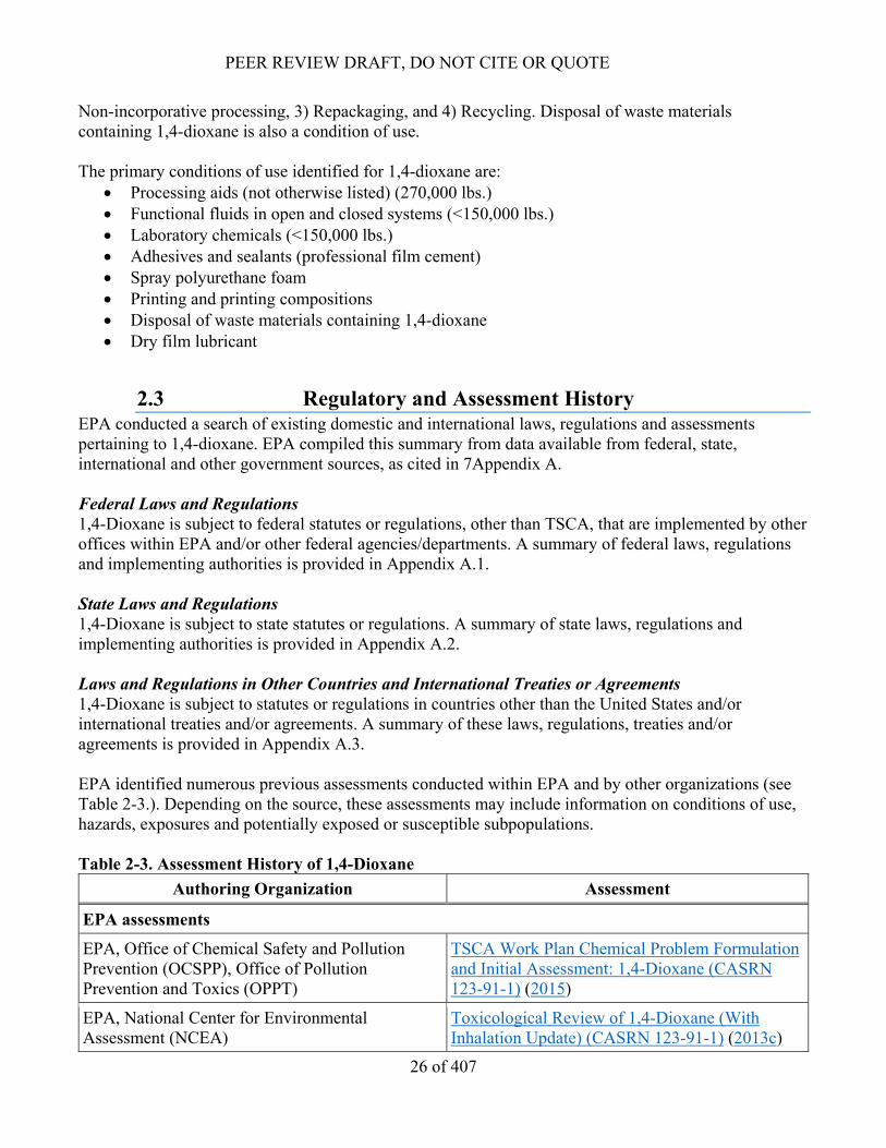
Non-incorporative processing, 3) Repackaging, and 4) Recycling. Disposal of waste materials containing 1,4-dioxane is also a condition of use. The primary conditions of use identified for 1,4-dioxane are:
• Processing aids (not otherwise listed) (270,000 lbs.) • Functional fluids in open and closed systems (<150,000 lbs.) • Laboratory chemicals (<150,000 lbs.) • Adhesives and sealants (professional film cement) • Spray polyurethane foam • Printing and printing compositions • Disposal of waste materials containing 1,4-dioxane • Dry film lubricant
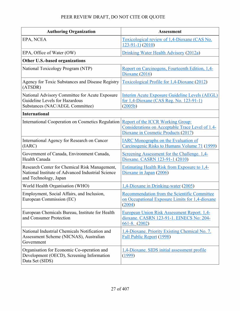
2.3 Regulatory and Assessment History EPA conducted a search of existing domestic and international laws, regulations and assessments pertaining to 1,4-dioxane. EPA compiled this summary from data available from federal, state, international and other government sources, as cited in 7Appendix A. Federal Laws and Regulations 1,4-Dioxane is subject to federal statutes or regulations, other than TSCA, that are implemented by other offices within EPA and/or other federal agencies/departments. A summary of federal laws, regulations and implementing authorities is provided in Appendix A.1. State Laws and Regulations 1,4-Dioxane is subject to state statutes or regulations. A summary of state laws, regulations and implementing authorities is provided in Appendix A.2. Laws and Regulations in Other Countries and International Treaties or Agreements 1,4-Dioxane is subject to statutes or regulations in countries other than the United States and/or international treaties and/or agreements. A summary of these laws, regulations, treaties and/or agreements is provided in Appendix A.3. EPA identified numerous previous assessments conducted within EPA and by other organizations (see Table 2-3.). Depending on the source, these assessments may include information on conditions of use, hazards, exposures and potentially exposed or susceptible subpopulations. Table 2-3. Assessment History of 1,4-Dioxane
Authoring Organization Assessment
EPA assessments
EPA, Office of Chemical Safety and Pollution Prevention (OCSPP), Office of Pollution Prevention and Toxics (OPPT)
TSCA Work Plan Chemical Problem Formulation and Initial Assessment: 1,4-Dioxane (CASRN 123-91-1) (2015)
EPA, National Center for Environmental Assessment (NCEA)
Toxicological Review of 1,4-Dioxane (With Inhalation Update) (CASRN 123-91-1) (2013c)
International Cooperation on Cosmetics Regulation Report of the ICCR Working Group: Considerations on Acceptable Trace Level of 1.4-Dioxane in Cosmetic Products (2017)
International Agency for Research on Cancer (IARC)
IARC Monographs on the Evaluation of Carcinogenic Risks to Humans Volume 71 (1999)
Government of Canada, Environment Canada, Health Canada
Screening Assessment for the Challenge. 1,4-Dioxane. CASRN 123-91-1 (2010)
Research Center for Chemical Risk Management, National Institute of Advanced Industrial Science and Technology, Japan
Estimating Health Risk from Exposure to 1,4-Dioxane in Japan (2006)
World Health Organisation (WHO) 1,4-Dioxane in Drinking-water (2005)
Employment, Social Affairs, and Inclusion, European Commission (EC)
Recommendation from the Scientific Committee on Occupational Exposure Limits for 1,4-dioxane (2004)
European Chemicals Bureau, Institute for Health and Consumer Protection
European Union Risk Assessment Report. 1,4-dioxane. CASRN 123-91-1. EINECS No: 204-661-8. (2002)
National Industrial Chemicals Notification and Assessment Scheme (NICNAS), Australian Government
1,4-Dioxane. Priority Existing Chemical No. 7. Full Public Report (1998)
Organisation for Economic Co-operation and Development (OECD), Screening Information Data Set (SIDS)
Conditions of Use Included in the Risk Evaluation TSCA (15 U.S.C. § 2602(4)) defines the conditions of use as ‘‘the circumstances, as determined by the Administrator, under which a chemical substance is intended, known, or reasonably foreseen to be manufactured, processed, distributed in commerce, used, or disposed of.” The conditions of use are described below in Table 2-4. Information on an additional use was submitted to EPA during the public comment period for the problem formulation. Specifically, EPA received information indicating that the Department of Energy’s Kansas City National Security Campus uses 1,4-dioxane as a constituent of a dry film lubricant in the manufacture of components for weapons systems. Although not reflected in the problem formulation, this condition of use is included in this risk evaluation. The updated life cycle diagram is presented in Figure. No further evaluation of distribution of 1,4-dioxane was included in this risk evaluation because chemicals are packaged in closed-system containers during distribution in commerce and no exposures are expected. Consumer uses were not considered within scope of this risk evaluation per the problem formulation, which states that such activities will be considered in the scope of the risk evaluation for ethoxylated chemicals. EPA believes that its regulatory tools under TSCA section 6(a) are better suited to addressing any unreasonable risks that might arise from these activities through regulation of the activities that generate 1,4-dioxane as an impurity or cause it to be present as a contaminant than addressing them through direct regulation of 1,4-dioxane (U.S. EPA, 2018c). As described in the Problem Formulation, general population exposures were not evaluated based on EPA’s determination that the existing regulatory programs and associated analytical processes have addressed or are in the process of addressing potential risks of 1,4-dioxane that may be present in various media pathways (e.g., air, water, land) for the general population (U.S. EPA, 2018c). Closed system functional fluid precludes exposure as the transfer device could prohibit the escape of chemicals outside the system. Due to the lack of evidence supporting its intended use in closed system functional fluids, occupational exposures for functional fluid (closed system) of 1,4-dioxane were not assessed.
Figure 2-1. 1,4-Dioxane Life Cycle Diagram The life cycle diagram depicts the conditions of use that are within the scope of the risk evaluation during various life cycle stages including manufacturing, processing, use (industrial or commercial) and disposal. The production volumes shown are for reporting year 2015 from the 2016 CDR reporting period (U.S. EPA, 2016a). a See Table 2-4 for additional uses not mentioned specifically in this diagram.
Life Cycle Stage Category a Subcategory b References Public Comment, EPA-HQ-OPPT-2016-0723-0021
Other uses Spray polyurethane foam Printing and printing compositions, including 3D printing Dry film lubricant
Use document, EPA-HQ-OPPT-2016-0723-0003; Public Comment, EPA-HQ-OPPT-2016-0723-0012
Disposal Disposal Industrial pre-treatment
(U.S. EPA, 2017e)
Industrial wastewater treatment Publicly owned treatment works (POTW) Underground injection Municipal landfill Hazardous landfill Other land disposal Municipal waste incinerator Hazardous waste incinerator Off-site waste transfer
a These categories of conditions of use appear in the initial life cycle diagram, reflect CDR codes and broadly represent conditions of use for 1,4-dioxane in industrial and/or commercial settings. b These subcategories reflect more specific uses of 1,4-dioxane.
Conceptual Models The conceptual models for this risk evaluation are shown in Figures 2-2 and 2-3. EPA considered the potential for hazards to workers and occupational non-users (ONUs) from inhalation, workers dermal exposure and hazards to the environment resulting from exposure to aquatic species as shown in the preliminary conceptual models and analysis plan of the 1,4-dioxane scope document (U.S. EPA, 2017d). Workers, ONUs, and bystanders and certain other groups of individuals who may experience greater exposures than the general population due to proximity
to conditions of use to be potentially exposed or susceptible subpopulations. Workers and ONUs could be exposed via pathways that are distinct from the general population due to unique characteristics (e.g., life stage, behaviors, activities, duration) that increase exposure, and whether groups of individuals have heightened susceptibility. The conceptual models indicate the exposure pathways and exposure routes of 1,4-dioxane to workers from industrial and commercial activities, and environmental releases and wastes. The problem formulation documents refined the initial conceptual models and analysis plans that were provided in the scope documents (U.S. EPA, 2018c). EPA has included the mapping tables that described all possible scenarios and whether they would be further evaluated. This was developed during problem formulation and is presented in Appendix B. The environmental characterization for the pathways included in the risk evaluation is described in Section 5.1.
Figure 2-2. 1,4-Dioxane Conceptual Model for Industrial and Commercial Activities and Uses: Potential Exposures and Hazards The conceptual model presents the exposure pathways, exposure routes and hazards to human receptors from industrial and commercial activities and uses of 1,4-dioxane that EPA analyzed in this draft risk evaluation. a Additional uses of 1,4-dioxane are included in Table 2-4. b Fugitive air emissions are those that are not stack emissions (emissions that occur through stacks, confined vents, ducts, pipes or other confined air streams), and include fugitive equipment leaks from valves, pump seals, flanges, compressors, sampling connections, open-ended lines; evaporative losses from surface impoundment and spills; and releases from building ventilation systems. c Based on physical chemical properties, 1,4-dioxane in mists that deposit in the upper respiratory tract will likely be rapidly absorbed in the respiratory tract or evaporate and were considered in the inhalation exposure assessment. d Receptors include potentially exposed or susceptible subpopulations. e EPA also considered the effect that engineering controls and/or personal protective equipment (PPE) have on occupational exposure levels.
PEER REVIEW DRAFT, DO NOT CITE OR QUOTE
35 of 407
Figure 2-3. 1,4-Dioxane Conceptual Model for Environmental Releases and Wastes: Potential Exposures and Hazards The conceptual model presents the exposure pathways, exposure routes and hazards to human and environmental receptors from environmental releases and wastes of 1,4-dioxane that EPA analyzed in problem formulation. Analyses were conducted using physical and chemical properties, fate information and surface water modeling during problem formulation. EPA has included the results of the analyses in Section 3.3.1, Appendix D, and Appendix E) and risk characterizations based on these analyses are included in the risk characterization (Section 5.1). a Industrial wastewater or liquid wastes may be treated on-site and then released to surface water (direct discharge), or pre-treated and released to POTW (indirect discharge).
PEER REVIEW DRAFT, DO NOT CITE OR QUOTE
Page 36 of 407
2.5 Systematic Review TSCA requires EPA to use scientific information, technical procedures, measures, methods, protocols, methodologies and models consistent with the best available science and base decisions on the weight of the scientific evidence. Within the TSCA risk evaluation context, the weight of the scientific evidence is defined as “a systematic review method, applied in a manner suited to the nature of the evidence or decision, that uses a pre-established protocol to comprehensively, objectively, transparently, and consistently identify and evaluate each stream of evidence, including strengths, limitations, and relevance of each study and to integrate evidence as necessary and appropriate based upon strengths, limitations, and relevance” (40 C.F.R. 702.33). To meet the TSCA § 26(h) science standards, EPA used the TSCA systematic review process described in the Application of Systematic Review in TSCA Risk Evaluations document (U.S. EPA, 2018b). The process complements the risk evaluation process in that the data collection, data evaluation and data integration stages of the systematic review process are used to develop the exposure and hazard assessments based on reasonably available information. EPA defines “reasonably available information” to mean information that EPA possesses, or can reasonably obtain and synthesize for use in risk evaluations, considering the deadlines for completing the evaluation (Citation to Final Rule). EPA is implementing systematic review methods and approaches within the regulatory context of the amended TSCA. Although EPA will make an effort to adopt as many best practices as practicable from the systematic review community, EPA expects modifications to the process to ensure that the identification, screening, evaluation and integration of data and information can support timely regulatory decision making under the aggressive timelines of the statute.
Data and Information Collection EPA planned and conducted a comprehensive literature search based on key words related to the different discipline-specific evidence supporting the risk evaluation (e.g., environmental fate and transport; engineering releases and occupational exposure; exposure to general population, consumers and environmental exposure; and environmental and human health hazard). EPA then developed and applied inclusion and exclusion criteria during the title and abstract screening to identify information potentially relevant for the risk evaluation process. The literature and screening strategy as specifically applied to 1,4-dioxane is described in the Strategy for Conducting Literature Searches for 1,4-Dioxane: Supplemental File for the TSCA Scope Document and the results of the title and abstract screening process were published in the 1, 4-Dioxane (CASRN 123-91-1) Bibliography: Supplemental File for the TSCA Scope Document; (U.S. EPA, 2017a). For studies determined to be on-topic (or relevant) after title and abstract screening, EPA conducted a full text screening to further exclude references that were not relevant to the risk evaluation. Screening decisions were made based on eligibility criteria documented in the form of the populations, exposures, comparators, and outcomes (PECO) framework or a modified
framework1. Data sources that met the criteria were carried forward to the data evaluation stage. The inclusion and exclusion criteria for full text screening for 1,4-dioxane are available in Appendix F of the Problem Formulation of the Risk Evaluation for 1,4-Dioxane (U.S. EPA, 2018c). Although EPA conducted a comprehensive search and screening process as described above, EPA made the decision to leverage the literature published in previous assessments2 when identifying relevant key and supporting data3 and information for developing the 1,4-dioxane risk evaluation. This is discussed in the Strategy for Conducting Literature Searches for 1,4-Dioxane: Supplemental Document to the TSCA Scope Document . In general , many of the key and supporting data sources were identified in the comprehensive 1,4-Dioxane (123-91-1) Bibliography: Supplemental File for the TSCA Scope Document (U.S. EPA, 2017a). However, there were instances that EPA missed relevant references that were not captured in the initial categorization of the on-topic references. EPA found additional relevant data and information using backward reference searching, which was a technique that will be included in future search strategies. This issue was discussed in Section 4 of the Application of Systematic Review for TSCA Risk Evaluations. Other relevant key and supporting references were identified through targeted supplemental searches to support the analytical approaches and methods in the 1,4-dioxane risk evaluation (e.g., to locate specific information for exposure modeling) or to identify new data and information published after the date limits of the initial search. EPA used previous chemical assessments to quickly identify relevant key and supporting information as a pragmatic approach to expedite the quality evaluation of the data sources, but many of those data sources were already captured in the comprehensive literature as explained above. EPA also considered newer information not taken into account by previous chemical assessments as described in the Strategy for Conducting Literature Searches for 1,4-Dioxane: Supplemental Document to the TSCA Scope Document . EPA then evaluated the confidence of the key and supporting data sources as well as newer information instead of evaluating the confidence of all the underlying evidence ever published on a chemical substance’s fate and transport, environmental releases, environmental and human exposure and hazards. Such comprehensive evaluation of all of the data and information ever published for a chemical substance would be extremely labor intensive and could not be achieved under the TSCA statutory deadlines for most chemical substances especially those that have a data rich database. Furthermore, EPA evaluated how EPA’s evaluation of the key and supporting data and
1 A PESO statement was used during the full text screening of environmental fate and transport data sources. PESO stands for Pathways and Processes, Exposure, Setting or Scenario, and Outcomes. A RESO statement was used during the full text screening of the engineering and occupational exposure literature. RESO stands for Receptors, Exposure, Setting or Scenario, and Outcomes.
2 Examples of existing assessments are EPA’s chemical assessments (e.g. previous work plan risk assessments, problem formulation documents), ATSDR’s Toxicological Profiles, EPA’s IRIS assessments and ECHA’s dossiers. This is described in more detail in the Strategy for Conducting Literature Searches for 1,4-Dioxane: Supplemental File for the TSCA Scope Document (https://www.epa.gov/sites/production/files/2017-06/documents/14-dioxane_lit_search_strategy_053017.pdf).
3 Key and supporting data and information are those that support key analyses, arguments, and/or conclusions in the
information and newer information would change the previous conclusions presented in the previous assessments. Using this pragmatic approach, EPA evaluated the confidence of the key and supporting data sources as well as newer information instead of evaluating the confidence of all the underlying evidence ever published on 1,4-dioxane’s fate and transport, environmental releases, environmental and human exposure and hazards. This allowed EPA to maximize the scientific and analytical efforts of other regulatory and non-regulatory agencies by accepting for the most part the relevant scientific knowledge gathered and analyzed by others except for influential information sources that may have an impact on the weight of the scientific evidence and ultimately the risk findings. The influential information (i.e., key/supporting) came from a smaller pool of sources subject to the rigor of the TSCA systematic review process to ensure that the risk evaluation uses the best available science and the weight of the scientific evidence.
Figures 2-4, 2-5, 2-6, 2-7, and 2-8 depict the literature flow diagrams illustrating the results of this process for each scientific discipline-specific evidence supporting the draft risk evaluation. Each diagram provides the total number of references at the start of each systematic review stage (i.e., data search, data screening, data evaluation, data extraction/data integration) and those excluded based on criteria guiding the screening and data quality evaluation decisions. EPA made the decision to bypass the data screening step for data sources that were highly relevant to the draft risk evaluation as described above. These data sources are depicted as “key/supporting data sources” in the literature flow diagrams. Note that the number of “key/supporting data sources” were excluded from the total count during the data screening stage and added, for the most part, to the data evaluation stage depending on the discipline-specific evidence. The exception was the engineering releases and occupational exposure data sources that were subject to a combined data extraction and evaluation step (Figure 2-5).
Figure 2-4. Literature Flow Diagram for Environmental Fate and Transport Data Sources
Note: Following data screening, EPA determined during problem formulation that no environmental pathways would be further analyzed (U.S. EPA, 2018c). EPA evaluated a biodegradation study that was a key source in a previous EPA assessment (U.S. EPA, 2015) and is discussed in Section 3.1.
* These are key and supporting studies from existing assessments (e.g., EPA IRIS assessments, ATSDR assessments, ECHA dossiers) that were considered highly relevant for the TSCA risk evaluation. These studies bypassed the data screening step and moved directly to the data evaluation step.
Figure 2-5. Literature Flow Diagram for Engineering Releases and Occupational Exposure Data Sources.
Note: Key and supporting studies (n=14) were identified from existing assessments (e.g., EPA IRIS assessments, ATSDR assessments, ECHA dossiers) and were considered highly relevant for the TSCA risk evaluation. These studies bypassed the data screening step and moved directly to the data evaluation step. EPA conducted a literature search to determine relevant references for assessing engineering releases and occupational exposures for 1,4-dioxane within the scope of the risk evaluation. This search identified 2,981 references, including relevant supplemental documents. Of these, 2,967 were forwarded for screening of the title, abstract, and/or full text for an inclusion/exclusion (RESO) screening process for relevancy and quality. Of these, 98 references were recommended for data evaluation across up to four major study types, each with their respective evaluation metrics. Sixteen of these were forwarded for further extraction and data integration.
PEER REVIEW DRAFT, DO NOT CITE OR QUOTE
Page 40 of 407
Figure 2-6. Literature Flow Diagram for General Population, Consumer and Environmental Exposure Data Sources
Note: EPA’s problem formulation laid out the scope of the evaluation and used reasonably available sources of information to evaluate potential exposures to environmental receptors (aquatic) pathways from 1,4-dioxane. The confidence of these data sources was considered acceptable for risk evaluation purposes and thus they were used to support the analyses during scoping and problem formulation. EPA determined during problem formulation that environmental pathways were within scope but would not be further analyzed based on quantitative and qualitative analyses covering ecological pathways (U.S. EPA, 2018c). These analyses were made ahead of the data screening stage for these data sources, and therefore, all exposure references were excluded, as they did not meet the risk evaluation PECO statement.
Figure 2-7. Literature Flow Diagram for Environmental Hazard Data Sources
Note: The environmental hazard data sources were identified through literature searches and screening strategies using the ECOTOX Standing Operating Procedures. Additional details about the process can be found in the Strategy for Conducting Literature Searches for 1,4-Dioxane: Supplemental File for the TSCA Scope Document, EPA-HQ-OPPT-2016-0723. During problem formulation, EPA made refinements to the conceptual models resulting in the elimination of the terrestrial exposure pathway from further analysis. Thus, environmental hazard data sources on terrestrial organisms were considered out of scope and excluded from data quality evaluation.
PEER REVIEW DRAFT, DO NOT CITE OR QUOTE
Page 42 of 407
Figure 2-8. Literature Flow Diagram for Human Health Hazard Data Sources Note: Key and supporting studies (n=17) were identified from existing assessments (e.g., EPA IRIS assessments, ATSDR assessments, ECHA dossiers) and considered highly relevant for the TSCA risk evaluation. These studies bypassed the data screening step and moved directly to the data evaluation step.
Data Evaluation During the data evaluation stage, EPA assesses the quality of the data sources using the evaluation strategies and criteria described in the Application of Systematic Review in TSCA Risk Evaluations (U.S. EPA, 2018b). For the data sources that passed full-text screening and the key and supporting data sources, EPA evaluated their quality and each data source received an overall confidence of high, medium, low or unacceptable. The results of the data quality evaluations are summarized in Sections 3.1 (Fate and Transport), 3.2 (Releases to the Environment), 3.3 (Environmental Exposures), 3.4 (Human Exposures), 4.1 (Environmental Hazards) and 4.2 (Human Health Hazards). Additional information is provided in the appendices of the main document. Supplemental files4 also provide details of the data evaluations including individual metric scores and the overall study score for each data source.
4 There are various supplemental files accompanying the risk evaluation: • Risk Evaluation for 1,4-Dioxane, Systematic Review Supplemental File: Updates to the Data Quality Criteria for
Epidemiological Studies • Risk Evaluation for 1,4-Dioxane, Systematic Review Supplemental File: Data Quality Evaluation for Engineering Releases
and Occupational Exposure Data Sources • Risk Evaluation for 1,4-Dioxane, Systematic Review Supplemental File: Data Quality Evaluation of Environmental Hazard
Studies • Risk Evaluation for 1,4-Dioxane, Systematic Review Supplemental File: Data Quality Evaluation of Environmental Fate and
Transport Studies • Risk Evaluation for 1,4-Dioxane, Systematic Review Supplemental File: Data Quality Evaluation of Human Health Hazard
Studies, Animal and In Vitro Studies • Risk Evaluation for 1,4-Dioxane, Systematic Review Supplemental File: Data Quality Evaluation of Epidemiological
Data Integration Data integration includes analysis, synthesis and integration of information for the risk evaluation. During data integration, EPA considers quality, consistency, relevancy, coherence and biological plausibility to make final conclusions regarding the weight of the scientific evidence. As stated in the Application of Systematic Review in TSCA Risk Evaluations (U.S. EPA, 2018b), data integration involves transparently discussing the significant issues, strengths, and limitations as well as the uncertainties of the reasonably available information and the major points of interpretation (U.S. EPA, 2018d). EPA defines “reasonably available information” to mean information that EPA possesses, or can reasonably obtain and synthesize for use in risk evaluations, considering the deadlines for completing the evaluation (Procedures for Chemical Risk Evaluation Under the Amended Toxic Substances Control Act (82 FR 33726)). EPA used previous assessments (see Table 2-3) to identify key and supporting information and then analyzed and synthesized available evidence regarding 1,4-dioxane’s chemical properties, environmental fate and transport properties and its potential for exposure and hazard. EPA’s analysis also considered recent data sources that were not considered in the previous assessments (Section 0) as well as reasonably available information on potentially exposed or susceptible subpopulations. The exposures and hazards sections describe EPA’s analysis of the influential information (i.e., key and supporting data) that were found acceptable based on the data quality reviews as well as discussion of other scientific knowledge using the approach described in Section 0. The exposure section also describes whether aggregate or sentinel exposures to a chemical substance were considered under the conditions of use within the scope of the risk evaluation, and the basis for that consideration
3 EXPOSURES
3.1 Fate and Transport EPA gathered and evaluated environmental fate information according to the process described in the Application of Systematic Review in TSCA Risk Evaluations (U.S. EPA, 2018b). Reasonably available environmental fate data were selected for use in the current evaluation. Furthermore, EPA used previous regulatory and non-regulatory 1,4-dioxane assessments to inform the environmental fate and transport information discussed in this section and Appendix D. EPA had confidence in the information used in the previous assessments of 1,4-dioxane (see Table 2-3) to describe the environmental fate and transport of 1,4-dioxane and thus used it to make scoping decisions. Because EPA determined during problem formulation that no environmental pathways would be further analyzed, EPA limited data extraction and evaluation to key data sources used in previous assessments (see Table 2-3), as described in Section 2.5.2. Thus, EPA assessed the quality of a • Risk Evaluation for 1,4-Dioxane, Systematic Review Supplemental File: Data Quality Evaluation of Human Health Hazard
microcosm study on soil biodegradation (Kelley et al., 2001) based on the data quality criteria described in the Application of Systematic Review in TSCA Risk Evaluations (U.S. EPA, 2018b) and the study was rated ‘high’ confidence. The data evaluation tables describing review of the sources used in this assessment can be found in the supplemental document, Data Quality Evaluation of Environmental Fate and Transport Studies {U.S. EPA, 2019, HERO ID}. Other fate estimates were based on modeling results from EPI Suite™ (U.S. EPA, 2012c), a predictive tool for physical/chemical and environmental fate properties (https://www.epa.gov/tsca-screening-tools/epi-suitetm-estimation-program-interface). The inputs and setup of EPI Suite™ runs for 1,4-dioxane are described in Appendix D. EPI Suite™ was reviewed by the EPA Science Advisory Board (http://yosemite.epa.gov/sab/sabproduct.nsf/02ad90b136fc21ef85256eba00436459/CCF982BA9F9CFCFA8525735200739805/$File/sab-07-011.pdf) and the individual models have been peer-reviewed in numerous articles published in technical journals. Citations for such articles are available in the EPI Suite™ help files. The 1,4-dioxane environmental fate characteristics and physical-chemical properties used in fate assessment are presented in Table 3-1. EPA used EPI Suite™ estimations and reasonably available fate data to characterize the environmental fate and transport of 1,4-dioxane. As part of problem formulation, EPA also analyzed the sediment and land-applied biosolids pathways. The results of the analyses are described in the 2018 problem formulation for 1,4-dioxane (U.S. EPA, 2018c) and presented again in Appendix D. Please note that this section and Appendix D may also cite other data sources as part of the reasonably available information on the fate and transport properties of 1,4-dioxane. EPA did not subject these other data sources to the later phases of the systematic review process (i.e., data evaluation and integration) based on the approach explained above. Table 3-1. Environmental Fate Characteristics of 1,4-Dioxane
Property or Endpoint
Value a References Data Quality Rating
Direct photodegradation
Not expected to undergo direct photolysisb
(ToxNet Hazardous Substances Data Bank, 2017; U.S. EPA, 2015)
Not applicable
Indirect photodegradation
4.6 hours (estimated for atmospheric degradation)c
(U.S. EPA, 2015, 2012c)
High
Hydrolysis half-life Does not undergo hydrolysisb (U.S. EPA, 2015; Wilbur et al., 2012)
Not applicable
Biodegradation 0% in 120 days, 60% in 300 days (aerobic in soil microcosm)
a Measured unless otherwise noted. b1,4-Dioxane lacks functional groups susceptible to the degradation mechanism cInformation was estimated using EPI Suite™ (U.S. EPA, 2012c) The EPI Suite™ module that estimates chemical removal in sewage treatment plants (STPWIN) was run using default settings (details available in the STPWIN help file in EPI Suite™) and estimated that 0.3% of 1,4-dioxane in wastewater will be removed by volatilization while < 2% of 1,4-dioxane will be removed by adsorption. The organic carbon-water partition coefficient, log KOC, reported in previous assessments of 1,4-dioxane were in the range of 0.4 – 1.23 (U.S. EPA, 2013c; ATSDR, 2012; U.S. EPA, 2010; ECJRC, 2002; NICNAS, 1998), and log KOC values within this range are associated with low sorption to soil, sediment, and suspended solids. Aerobic biodegradation of 1,4-dioxane is slow or negligible (U.S. EPA, 2015; ATSDR, 2012; NTP, 2011; Health Canada, 2010; ECJRC, 2002; NICNAS, 1998) and will not contribute significantly to removal of 1,4-dioxane in wastewater treatment. Thus, concentrations of 1,4-dioxane in biosolids will be essentially equal to concentrations in the overlying wastewater, and the 1,4-dioxane contained in biosolids will almost all be in the aqueous phase rather than adsorbed to particles. Similarly, 1,4-dioxane concentrations in sediment are expected to be nearly equal to concentrations in overlying water, with 1,4-dioxane almost exclusively in the aqueous phase of sediment samples. Due to its water solubility (>800 g/L; Table 2-1) and Henry’s Law constant (4.8 × 10⁻⁶ atm-m3/mole at 25°C; Table 2-1), 1,4-dioxane is expected to demonstrate limited volatility from water surfaces, moist soil, and other moist surfaces such as land-applied biosolids. Once it enters the environment, 1,4-dioxane is not expected to significantly adsorb to suspended solids and sediment based on its log KOC and is therefore expected to migrate to surface waters and groundwater. 1,4-Dioxane is expected to volatilize from dry surfaces and dry soil due to its vapor pressure (40 mm Hg at 25°C). In the atmosphere, it is expected to react with hydroxyl radicals with an indirect photolysis half-life on the order of hours (U.S. EPA, 2012c). The estimated bioconcentration and bioaccumulation factors are 3 or below (Table 3-1) and measured bioconcentration factors for 1,4-dioxane are 0.7 or below (ECJRC, 2002). Therefore, 1,4-dioxane has low bioaccumulation potential.
Overall, 1,4-dioxane is not likely to accumulate in wastewater biosolids, sediment, soil, or biota, and is expected to largely remain in aqueous phases where it will slowly biodegrade or volatilize and then degrade by indirect photolysis.
3.2 Environmental Releases Releases to the environment from conditions of use (e.g., industrial and commercial processes) are one component of potential exposure and may be derived from reported data that are obtained through direct measurement, calculations based on empirical data and/or assumptions and models. Under the Emergency Planning and Community Right-to-Know Act (EPCRA) Section 313, 1,4-dioxane has been a Toxics Release Inventory (TRI)-reportable substance since 1987. The TRI database includes information on disposal and other releases of 1,4-dioxane to air, water, and land, in addition to how it is being managed through recycling, treatment, and burning for energy recovery. Based on 2015 TRI reporting, an estimated 35,402 lbs. of 1,4-dioxane was released to surface water from industrial sources. See Table E-1 in Appendix E for a TRI summary table and further details on recent releases of 1,4-dioxane to various media.
3.3 Environmental Exposures In the problem formulation, EPA presented an analysis on environmental exposures to aquatic species based on releases to surface water. No additional information was received or identified by the EPA following the publication of the problem formulation that would alter the analysis and interpretations presented in the problem formulation. As reviewed during problem formulation, 1,4-dioxane is present in environmental media such as groundwater, surface water, and air. EPA conducted analysis of the environmental release pathways based on a qualitative assessment of the physical-chemical properties and fate of 1,4-dioxane in the environment (described in Section 3.1), and a quantitative comparison of hazards and exposures for aquatic organisms as described in Section 4.1.2 of the problem formulation (U.S. EPA, 2018c).
Environmental Exposures – Aquatic Pathway As described in the problem formulation (U.S. EPA, 2018c), an aquatic exposure assessment was conducted using TRI and DMR release information to model predicted surface water concentrations near discharging facilities. To examine whether near-facility surface water concentrations could approach 1,4-dioxane’s concentrations of concern, EPA employed a conservative approach, using available modeling tools and data to estimate near-facility surface water concentrations resulting from reported releases of 1,4-dioxane to surface water. High-end surface water concentrations (i.e., those obtained assuming low receiving water body stream flows) from all E-FAST 2014 (U.S. EPA, 2014c) runs ranged from 0.006 µg/L to 11,500 µg/L. National-scale monitoring data from EPA’s STOrage and RETreival (STORET) and National Water Information System (NWIS) for the past ten years, shows that 1,4-dioxane is detected in surface water. The data points show a detection rate of approximately 6% for this media, with detections ranging from 0.568 to 100 µg/L. The E-FAST results and monitoring data were compared to the acute and chronic aquatic concentrations of concern of 247,200 µg/L and 14,500 µg/L, respectively (see section 4.1). This aquatic exposure analysis and additional details about
the approach and results are presented in and Appendix E. The analysis and determination of risk are presented in the risk characterization and risk determination sections, respectively.
3.4 Human Exposures
Occupational Exposures Occupational exposures could be direct or indirect and the magnitude of exposure for an occupational worker could be a function of timeframe of exposures. The timeframes of exposure, which depend on occupational mobility, could vary for different population groups. ONUs are workers at the facility who are neither directly perform activities near the 1,4-dioxane source area not regularly handle 1,4-dioxane. The job classifications for ONUs could be dependent on the conditions of use. For example, ONUs for manufacturing include supervisors, managers, and tradesmen that may be in the manufacturing area, but do not perform tasks that result in the same level of exposures as production workers. It could be challenging to characterize direct and indirect exposures to contaminants since it is not uncommon for employees at certain facility to perform multiple types of tasks throughout the work day. The workers could perform activities that bring them into direct contact with 1,4-dioxane and they could also perform additional tasks as ONUs. The groupings of employees are not necessarily distinct as workers perform a variety of tasks over the course of the day that could result in direct exposure and indirect exposure throughout the day. Indirect exposures of employees working near contaminants could be difficult to separate due to overlapping tasks that makes it difficult to delineate exposures of workers and ONUs. EPA evaluated acute and chronic inhalation exposures to workers and ONUs in association with 1,4-dioxane manufacturing, import and repackaging, its use in industrial applications, open system functional fluids, spray polyurethane foam insulation, laboratory chemicals, film cement, printing inks (3D), dry film lubricant, and disposal. Appendix G.6 provides additional detail on the mapping of the conditions of use to the Occupational Exposure Scenario (OES) groups used in this risk evaluation. EPA used inhalation monitoring data from literature sources where available and that met data evaluation criteria (see Section 2.5); and modeling approaches to estimate potential inhalation exposures where inhalation monitoring data were not available. EPA modeled inhalation exposures using the following models: the EPA AP-42 Loading Model, the EPA Mass Balance Inhalation Model, and the EPA Total PNOR PEL-Limiting Model. More information about these models may be found in Section 3.4.1.1. EPA also estimated dermal doses for workers in these scenarios since dermal monitoring data was not reasonably available. EPA modeled dermal doses using the EPA Dermal Exposure to Volatile Liquids Model which improves upon the existing EPA 2-Hand Dermal Exposure model by accounting for the effect of evaporation on dermal absorption for volatile chemicals and the potential exposure reduction due to glove use. More information about this model and how it was used may be found in Section 3.4.1.14 and Appendix G.7. EPA does not expect dermal exposures for occupational non-users due to no direct contact with the chemical. Components of the Occupational Exposure Assessment The occupational exposure assessment for each condition of use comprises the following components:
PEER REVIEW DRAFT, DO NOT CITE OR QUOTE
Page 48 of 407
• Process Description of the condition of use, including the role of the chemical in the use; process vessels, equipment, and tools used during the condition of use; and descriptions of the worker activities, including an assessment for potential points of worker exposure.
• Number of Sites that use the chemical for the given condition of use. • Number of Workers and ONUs potentially exposed to the chemical for the given
condition of use. CDR data to identify the number of sites where exposure may occur and approximate workers who may be exposed to the chemicals. Unless mentioned otherwise in this report, the total number of workers and ONUs are number of personnel per site per day. The details on estimation of the number of workers and ONUs are discussed in Sections 3.4.1.1 and each conditions of use, and Appendix G.5.
• Central tendency and high-end estimates of inhalation exposure to workers and occupational non-users. See Section 3.4.1.1 for a discussion of EPA’s statistical analysis approach for assessing inhalation exposure.
• Dermal Exposure estimates for multiple scenarios, accounting for simultaneous absorption and evaporation, and different protection factors of glove use. The OSHA Personal Protective Equipment Standard, 29 CFR § 1910.132, requires that employers provide personal protective equipment such as hard hats, goggles, gloves, and respirators to protect employees from hazardous exposures. The OSHA recommends employers utilize the hierarchy of controls for reducing or removing hazardous exposures. The most effective controls are elimination, substitution, or engineering controls. 29 CFR § 1910.134(a)(1) establishes OSHA’s hierarchy of controls by requiring the use of feasible engineering controls as the primary means to control air contaminants. Respirators are required when effective engineering controls are not feasible. Gloves and other PPE are the last means of worker protection in the hierarchy of controls. When effective engineering and administrative controls are not feasible to adequately protect the health of workers and maintain compliance with other OSHA statutory and regulatory requirements under 29 CFR § 1910.1000, employers could provide PPE to protect employees (29 CFR § 1910.134(a)(1)).
• Users include female and male adult workers (>16 years old) exposed to 1,4-dioxane for 8‐hour exposure
• ONUs include female and male adult workers (>16 years old) exposed to 1,4-dioxane indirectly by being in the same work area of the building.
3.4.1.1 Occupational Exposures Approach and Methodology EPA performed a literature search to find descriptions of processes involving 1,4-dioxane and worker activities that could potentially result in occupational exposures. The on-topic sources were then screened against inclusion criteria in the RESO (Receptors, Exposures, Setting/Scenario, Outcomes) statement and the relevant sources were further evaluated using the data quality criteria in the Application of Systematic Review in TSCA Risk Evaluations (U.S. EPA, 2018b). EPA identified 98 potentially useful sources based on literature search, of which 65 sources were determined to have potentially useful exposure information (see Figure 2-5). Sources with an overall confidence score of less than 4 were considered acceptable in the systematic review. Of these 65 sources, 27 were deemed to be acceptable. Sixteen of the acceptable sources were determined to have exposure data relevant to the conditions of use and were therefore used in this evaluation. A summary of the data quality evaluation results for the 1,4-dioxane occupational exposure sources are presented in Appendix G.1 (“Systematic Review
Supplemental File for the TSCA Risk Evaluation: Data Quality Evaluation for Occupational Exposure and Release Data”). For the integration of occupational exposure data/information, EPA considered any relevant data that it determined to be acceptable for use. The hierarchy found later in this section under “General Inhalation Exposures Approach and Methodology” presents the preferences among the primary types of data/information to be analyzed, synthesized and integrated for the occupational exposure assessments in this risk evaluation. Additional Data Sources EPA used a variety of sources to supplement the data found through the Systematic Review process. The additional sources included relevant NIOSH Health Hazard Evaluations, Generic Scenarios, and Emission Scenario Documents. These sources were sometimes used to provide process descriptions of the conditions of use as well as estimates for the number of sites and worker counts. CDR data was also used to provide a basis to estimate the numbers of sites, workers, and ONUs. EPA supplemented the available CDR data with U.S. economic data using the following methods:
1. Identification of the North American Industry Classification System (NAICS) codes for the industry sectors associated with these uses.
2. Estimation of total employment by industry/occupation combination using the Bureau of Labor Statistics’ Occupational Employment Statistics (OES) data (BLS, 2016).
3. Refinement of the OES estimates where they are not sufficiently detailed by using the U.S. Census’ Statistics of US Businesses (SUSB) (U.S. Census Bureau, 2016a) data on total employment by 6-digit NAICS.
4. Use market penetration data (where available) to estimate the percentage of employees likely to be using 1,4-dioxane instead of other chemicals.
5. Combine the data generated in Steps 1 through 4 to produce an estimate of the number of establishments and employees using 1,4-dioxane in each industry/occupation combination, and sum these to arrive at a total estimate of the number of employees with exposure.
Market penetration data for 1,4-dioxane were not available for any condition of use. Without these data, it is unknown what portion of a given set of sites use 1,4-dioxane. Absent this information, EPA generally assumes that all sites involve 1,4-dioxane. Therefore, site, worker, and ONU numbers considered could be overestimated. General Dermal Exposures Approach and Methodology EPA estimated dermal exposures using the EPA Dermal Exposure to Volatile Liquids Model. This model accounts for evaporation, and glove usage which may provide a more refined estimate of exposure than the existing EPA 2-Hand Dermal Exposure model. Additional details about how this model was used is in Section 3.4.1.14. General Inhalation Exposures Approach and Methodology EPA developed occupational exposure values representative of central tendency conditions and
high-end conditions. A central tendency was assumed to be representative of occupational exposures in the center of the distribution for a given condition of use. EPA used the 50th percentile (median), mean (arithmetic or geometric), or mode of a distribution as representative of the central tendency scenario. EPA’s preference was to provide the 50th percentile of the distribution. However, if the full distribution was not known, EPA assumed that the mean, mode, or midpoint of the distribution represented the central tendency depending on the statistics available for the distribution (U.S. EPA, 1992). A high-end exposure estimate was defined to be representative of occupational exposures that occur at probabilities above the 90th percentile but below the 99.9th percentile, the exposure of the individual with the highest exposure (U.S. EPA, 1992). EPA considered high-end results at the 95th percentile. If the 95th percentile was not available, EPA used a different percentile greater than or equal to the 90th percentile but less than or equal to the 99.9th percentile, depending on the statistics available for the distribution. If the full distribution was not known and the preferred statistics were not available, EPA estimated a maximum or bounding estimate in lieu of the high-end occupational exposure estimates. In each case, EPA makes clear the actual percentile that was used. For occupational exposures, EPA used measured or modeled air concentrations to calculate exposure concentration metrics essential for risk assessment. These exposures are presented as 8-hour time weighted averages (TWAs) and used to calculate acute exposure concentrations (AECs), average daily concentrations (ADCs), and lifetime average daily concentrations (LADCs). The ADC is used to estimate chronic, non-cancer risks and the LADC is used to estimate chronic, cancer risks. These calculations required additional parameter inputs, such as years of exposure, exposure duration and frequency, and lifetime years. See Appendix G.2 for more information about parameters and equations used to calculate acute and chronic exposures. For the final exposure result metrics, each of the input parameters (e.g., air concentrations, working years, exposure frequency, lifetime years) were point estimates (i.e., a single descriptor or statistic, such as central tendency or high-end). EPA estimated a central tendency and high-end for each final exposure result metric using deterministic calculations and combinations of point estimates of each parameter. EPA documented the method and rationale for selecting parametric combinations to be representative of central tendency and high-end. A probabilistic approach was generally not used in cases where monitoring-based data was available, but models for that condition of use were not.
EPA followed the hierarchy below in selecting data and approaches for assessing inhalation exposures. In the hierarchy, monitoring data is preferred over modeling approaches and occupational exposure limits are least preferred. Within each of the three categories, the sources are listed in a descending order of preference. For example, 1a is preferred over 1b. Once a satisfactory source of information is identified in this list, sources below that point are not used, although they can provide useful information for other purposes of this evaluation. For example, if 1a satisfies the data needs, no other sources of data in this hierarchy are typically used for purposes of assessing inhalation exposures. However, if the quality of data is deemed too low or uncertain, EPA will not use those data and will provide justification.
1) Monitoring data: a) Personal samples from directly applicable scenarios (e.g. personal breathing zone,
PBZ, non-CBI data from BASF for the Manufacturing Scenario) b) Area samples from directly applicable scenarios (e.g. area data from a NIOSH
HHE for the Film Cement Scenario) c) Personal samples from potentially applicable or similar scenarios (e.g. PBZ data
from a manufacturing site that makes a chemical with physical properties similar to 1,4-dioxane)
d) Area samples from potentially applicable or similar scenarios (e.g. area data from a site that processes a chemical with physical properties similar to 1,4-dioxane)
2) Modeling approaches: a) Surrogate monitoring data from chemicals with similar properties. Surrogate data
was used to estimate the inhalation exposure from the thickness verification step in the Spray Foam Application condition of use. Appendix G.6.7 provides more details on this use of surrogate data.
b) Fundamental modeling approaches (e.g. modeling of the Spray Foam Application Scenario)
c) Statistical regression modeling approaches 3) Occupational exposure limits:
a) Company-specific OELs (for site-specific exposure assessments, e.g., there is only one manufacturer who provides to EPA their internal OEL but does not provide monitoring data)
b) OSHA PEL c) Other occupational exposure limits (ACGIH TLV, NIOSH REL, Occupational
Alliance for Risk Science (OARS) workplace environmental exposure level (WEEL) [formerly by AIHA])
EPA reviewed workplace inhalation monitoring data collected by government agencies such as OSHA and NIOSH, and monitoring data found in published literature (i.e., personal exposure monitoring data and area monitoring data). Studies were evaluated using the evaluation strategies laid out in the Application of Systematic Review in TSCA Risk Evaluations (U.S. EPA, 2018b). The supplemental file provides details of the data evaluations, including scores for each metric and the overall study score for each information source. Exposure values were calculated from the datasets provided in the sources depending on the size of the dataset. For datasets with six or more data points (Hawkins et al., 1992 ; U.S. EPA, 1994), central tendency and high-end exposures were estimated using the 50th percentile and 95th percentile. For datasets with three to five data points, central tendency exposure was calculated using the 50th percentile and the maximum was presented as the high-end exposure estimate. These data sets are considered to have relatively more uncertainty than datasets with more datapoints. For datasets with two data points, the midpoint was presented as a midpoint value and the higher of the two values was presented as a higher value. These data sets are generally considered to have high uncertainty. Finally, data sets with only one data point are considered indicating appropriate rationale, but EPA cannot determine the statistical representativeness of the values given the small sample size. Existing data collected on workers and at locations with a greater-than-average potential for high exposures, under certain conditions, could have
performed using a work/research plan as monitoring is generally performed when there are questions concerning compliance with industrial hygiene standards. As such these data sets are considered to have extremely high uncertainty associated with them. Specific details related to each condition of use can be found in Sections 3.4.1.2 - 3.4.1.13. For each condition of use, these values were used to calculate chronic (non-cancer and cancer) exposures. Equations and sample calculations for chronic exposures can be found in Appendix G.3. EPA estimated exposures using the following models when exposure monitoring data were unavailable:
• EPA AP-42 Loading Model estimates vapor releases that occur when vapor is displaced by liquid during container loading. It calculates a vapor generation rate (G) using the physio-chemical properties of the chemical (U.S. EPA, 2013b).
• EPA Mass Balance Inhalation Model estimates occupational inhalation exposures assuming the air immediately around the source of exposure behaves as a well-mixed zone. EPA used the vapor generation rate (G), calculated using the EPA AP-42 Loading Model, in conjunction with this model to develop estimates of inhalation exposure (U.S. EPA, 2013b).
• EPA Total PNOR PEL-Limiting Model estimates occupational inhalation exposures to particulates containing the chemical. The estimate assumes that the worker exposure is equal to the OSHA Permissible Exposure Limit (PEL) for Particulates, Not Otherwise Regulated (PNOR), total particulate (U.S. EPA, 2013b).
Specific descriptions of the use of these models for each condition of use can be found in Sections 3.4.1.2 - 3.4.1.13. Respiratory Protection OSHA’s Respiratory Protection Standard (29 CFR § 1910.132) provides a summary of respirator types by their assigned protection factor (APF). OSHA defines the APF to mean: the workplace level of respiratory protection that a respirator or class of respirators is expected to provide to employees when the employer implements a continuing, effective respiratory protection program according to the requirements of the OSHA Respiratory Protection Standard. OSHA recommends employers utilize the hierarchy of controls for reducing or removing hazardous exposures. The most effective controls are elimination, substitution, or engineering controls. Respirators, and any other personal protective equipment, are the last means of worker protection in the hierarchy of controls and should only be considered when process design and engineering controls cannot reduce workplace exposure to an acceptable level. Exposure to 1,4-dioxane can cause irritation and is likely carcinogenic (ATSDR, 2012; Wilbur et al., 2012). The United States has several regulatory and non-regulatory exposure limits for 1,4-dioxane: an OSHA PEL of 100 ppm 8-hour TWA (360 mg/m3) with a skin notation, a NIOSH Recommended Exposure Limit (REL) of 1 ppm (3.6 mg/m3) as a 30-minute ceiling and an American Conference of Government Industrial Hygienists (ACGIH) Threshold Limit Value (TLV) of 20 ppm TWA (72 mg/m3) (OSHA, 2005). If respirators are necessary in atmospheres that are not immediately dangerous to life or health, workers must use NIOSH-certified air-purifying respirators or NIOSH-approved supplied-air respirators with the appropriate APF. Respirators that meet these criteria include air-purifying respirators with organic vapor
cartridges. Respirators must meet or exceed the required level of protection listed in Table 3-2 to meet NIOSH recommended a 1 ppm (3.6 mg/m³, 30 minute) ceiling because 1,4-dioxane is a potential human carcinogen (29 CFR § 1990). The respirators should be used when effective engineering controls are not feasible as per OSHA’s 29 CFR § 1910.132. The knowledge of the range of respirator APFs is intended to assist employers in selecting the appropriate type of respirator that could provide a level of protection needed for a specific exposure scenario. Table 3-2 lists the range of APFs for respirators. The complexity and burden of wearing respirators increases with increasing APF. The APFs are not to be assumed to be interchangeable for any conditions of use, any workplace, or any worker or ONU. The use of a respirator not necessarily would resolve inhalation exposures since it cannot be assumed that employers have or will implement comprehensive respiratory protection programs for their employees. Table 3-2. Assigned Protection Factors for Respirators in OSHA Standard 29 CFR § 1910.132 Type of Respirator Quarter
• Pressure-demand or other positive-pressure mode (e.g., open/closed circuit)
10,000 10,000
Source: 29 CFR § 1910.132 Estimating the Number of Workers and Occupational Non-Users (ONUs) EPA used a method consisting of the following steps to estimate the number of workers and ONUs who may be potentially exposed to 1,4-dioxane in each condition of use:
1. Identify the North American Industry Classification System (NAICS) codes for the industry sectors associated with each condition of use.
2. Estimate total employment by industry/occupation combination using the Bureau of Labor Statistics’ Occupational Employment Statistics (OES) data (BLS, 2016).
3. Refine the OES estimates where they are not sufficiently granular by using the U.S. Census’ (2016b) Statistics of U.S. Businesses (SUSB) data on total employment by 6-digit NAICS.
4. Estimate the percentage of employees likely to be using 1,4-dioxane instead of other chemicals (i.e., the market penetration of 1,4-dioxane in the condition of use).
5. Estimate the number of sites and number of potentially exposed employees per site. 6. Estimate the number of potentially exposed employees within the condition of use.
See Appendix G.5 for more information about the approach used to estimate potentially exposed workers and ONUs.
3.4.1.2 Manufacturing 1,4-Dioxane is commercially manufactured by the acid-catalyzed dehydration of diethylene glycol, which in turn is obtained from the hydrolysis of ethylene oxide. The information and data quality evaluation to assess occupational exposures during manufacturing is listed in Table 3-3. See Appendix G.1 for additional details. Table 3-3. Manufacturing Worker Exposure Data Evaluation
Worker Activity or Sampling Location Data Type Number of
Samples Data Quality Rating Source Reference
Unknown PBZ Monitoring 28 High (BASF, 2016)
Routine duties, neutralization,
evaporator dump PBZ Monitoring 4 High (BASF, 2017)
N/A CDR Data – Number of sites and workers N/A High (U.S. EPA, 2016a)
Occupational exposures to 1,4-dioxane during manufacturing were estimated by evaluating full-shift, personal breathing zone (PBZ) monitoring data obtained by BASF during internal industrial hygiene (IH) studies. BASF monitoring data was selected as it is more relevant and recent compared to the manufacturing data cited in other sources [such as (ECJRC, 2002)] and lack of availability of monitoring data from other U.S. manufacturer. For example, the data cited in the 2002 EU Risk Assessment ranges from 1976 to 1998 while the data provided by BASF ranged from 2006 to 2017 (BASF, 2017, 2016; ECJRC, 2002). There was a lack of available monitoring data from the other known U.S. manufacturer. The BASF data had limitations including lack of descriptions of worker tasks, exposure sources, and possible engineering controls. The BASF (2016) workplace monitoring data appeared to be real-time PBZ exposure measurements. The data were assumed to be relevant to worker activities and were 8-hour TWA measurements. EPA estimated the total number of workers who could be potentially exposed as 78 and the number occupational non-users as 36 (U.S. EPA, 2016a). Acute and chronic occupational inhalation exposures during manufacturing of 1,4-dioxane are summarized in Table 3-4. EPA calculated the 95th percentile and 50th percentile of the available 30 data points for inhalation exposure monitoring data to assess the high-end and central tendency exposures, respectively. Using these 8-hour TWA exposure concentrations, EPA calculated the ADC and LADC using the equations in Appendix G.2. Additional information regarding the calculations is provided in Appendix G.6.1.
Table 3-4. Acute and Chronic Inhalation Exposures of Worker for Manufacturing Based on Monitoring Data
Exposure Type Central Tendency (50th percentile)
(mg/m3)
High-end (95th Percentile)
(mg/m3)
Data Quality Rating of Associated Source a
15-minute TWA (Evaporator Dump) N/A 137* High
8-hour TWA Exposure Concentrations 0.42 7.7 High
8-hour TWA Acute Exposure Concentration (AEC) 0.42 7.7 High
Average Daily Concentration (ADC) 0.40 7.4 High
Lifetime Average Daily Concentration (LADC) 0.16 3.8 High
N/A = not applicable. *: The higher of the two reported (BASF, 2017) 15-minute short-term exposures values (137 mg/m3 from the evaporator dump step), considered as high-end, short-term exposure. a See Table 3-3 for corresponding references. EPA estimated that 78 workers and 36 ONUs could be exposed at sites that manufacture 1,4-dioxane in the U.S. EPA used worker number estimates reported in CDR and refined them using BLS and SUSB data for the applicable NAICS codes. Additional information about the steps used to estimate the number of potentially exposed workers and ONUs are available in Appendix G.5. Exposure data for ONUs were not available. ONUs include employees that work at the site where 1,4-dioxane is manufactured, but unlike workers, they do not directly handle the chemical and are not near the chemical release source of the manufacturing process. Thus, ONUs are likely to have lower exposures than workers. ONUs for manufacturing include supervisors, managers, and tradesmen that may be in the manufacturing area, but do not perform tasks that result in the same level of exposures as production workers. Key Uncertainties The data sets used mostly lacked specific descriptions of worker tasks, exposure sources, and possible engineering controls to provide context. EPA assumed that the 2016 BASF data are PBZ measurements relevant to worker activities and are also 8-hour TWA measurements. This assumption could underestimate exposures. The sampling rate was missing for some of the 2016 data, so EPA assumed the same sampling rate was applied for other data in the set. It is uncertain to what extent the limited monitoring data used to estimate inhalation exposures for this scenario that could be representative of occupational exposures in other manufacturing facilities of 1,4-dioxane.
3.4.1.3 Import and Repackaging The import of chemicals, such as 1,4-dioxane, involves activities of handling of chemical during storage, transportation, distribution, and packaging and processing. In addition, 1,4-dioxane shipped in bulk containers could be repackaged into smaller containers for resale, such as drums or bottles using automatic, semi-automatic, or manual filling, sealing, labeling, and wrapping. The shipment methods and regulations of 1,4-dioxane require the material to be properly classed, described, packaged, marked, labeled, and in condition for shipment as required or authorized by the hazardous materials regulations (49 CFR § 171-177). To avoid
spilling, 1,4-dioxane needs to be transported in securely sealed glass bottles or equivalent containers that should themselves be placed inside strong screw-cap or snap-top container that will not open when dropped. Both the bottle and the outside container should be appropriately labelled. Airtight packaging is required by the International Labor Organization’s (ILO) International Chemical Safety Cards (ICSC). The information and data quality evaluation to assess occupational exposures from import and repackaging is listed in Table 3-5. See Appendix G.1 for more details about the data quality evaluation. Table 3-5. Import and Repackaging Data Source Evaluation
Worker Activity or Sampling Location Data Type Number of Samples Data Quality Rating Source Reference
N/A CDR Data – Number of sites and workers N/A High (U.S. EPA, 2016a)
EPA modeled central tendency and high-end occupational inhalation exposures for this scenario using the EPA AP-42 Loading Model and the EPA Mass Balance Inhalation Model (U.S. EPA, 2013b) and the values listed in Appendix G.2. EPA used a Monte Carlo simulation to vary the saturation factor (f), ventilation rate (Q), and mixing factor (k) and calculated the 95th percentile and 50th percentile exposures during unloading directly in the simulation to assess the high-end and central tendency exposures, respectively. See Appendix G.4 for more information about the Monte Carlo simulation. Since some sites may only repackage into either bottles or drums and some sites may use both types of containers, EPA estimated exposures for both bottles and drums. EPA used these values to calculate acute and chronic inhalation exposures in the Monte Carlo simulation, varying working years (WY) and the number of days, using the equations in Appendix G.2. EPA determined once per day short-term exposures of 170 to 610 mg/m3 with a duration of 30 minutes may occur during drum unloading as central tendency and high-end short-term exposures. These estimates are presented in Table 3-6. EPA estimated that the total number of potentially exposed workers could be between 38 to 149 workers, and occupational non-users could be between 12 to 49. EPA used worker number estimates reported in CDR and refined them using BLS and SUSB data for the applicable NAICS codes. See Appendix G.5 for more information about the steps used to estimate the number of potentially exposed workers and ONUs. Additional information including specific methodology and assumptions for modeling exposures are described in Appendix G.6.2.
Average Daily Concentration (ADC) 0.46 3.4 N/A - Modeled Data
Lifetime Average Daily Concentration (LADC) 0.18 1.3 N/A - Modeled Data
a See Table 3-5 for corresponding references. Exposure data for ONUs were not available. The ONU exposures are anticipated to be lower than worker exposures, since ONUs do not typically directly handle the chemical. Only inhalation exposures to vapors or incidental dermal exposures could be applicable to ONUs, which will likely be less than worker exposures. Key Uncertainties EPA modeled inhalation exposures using the EPA AP-42 Loading Model and the EPA Mass Balance Inhalation Model. Process specifics for import and repackaging at these sites were not available, therefore, EPA assumed certain process details, such as container sizes and loading and unloading frequency. Additionally, EPA assumed that the process steps associated with this scenario occur indoors, without engineering controls, and in an open-system environment where vapors freely escape. In the absence of industry-specific information, these assumptions provide for conservative estimates for exposures during this operation. Actual exposures may be less due to various factors including closed-system loading and unloading, the use of vapor recovery systems, or the automation of various process steps.
3.4.1.4 Recycling In the Problem Formulation of the Risk Evaluation for 1,4-Dioxane (U.S. EPA, 2018c), EPA identified recycling as a separate occupational exposure scenario. After further review, EPA assessed the recycling process as part of the Industrial Uses group, described in Section 3.4.1.5. Any exposures from worker activities, such as unloading, maintenance, and drumming spent 1,4-dioxane for disposal are assessed in Section 3.4.1.5.
3.4.1.5 Industrial Uses 1,4-Dioxane is used as a process solvent, an intermediate, and a catalyst in several industrial applications. For this assessment, these uses have been grouped into a broad category called “industrial uses.” The relevant industries and uses include the following:
• Process solvent in pharmaceutical and medicine manufacturing; • Process solvent in basic organic chemical manufacturing; • Wetting and dispersing agent in textile processing; • Wood pulping; • Extraction of animal and vegetable oils; • Purification of pharmaceuticals; • Etching of fluoropolymers; • Pharmaceutical intermediate; • Agricultural chemical intermediate; • Polymerization catalyst; • Plasticizer intermediate; • Plastics modeling (thermoforming); and • Catalysts and reagents for anhydrous acid reactions, brominations, and sulfonations.
EPA did not find specific details for most of these processes, but typical operations are expected to be similar across these uses. For uses grouped in this “industrial uses” category, it is expected that 1,4-dioxane is received as a solvent, intermediate, or catalyst in its final formulation and requires no further processing. The 1,4-dioxane is unloaded and charged to intermediate storage or directly used in the process. If it is being used as an intermediate, it will likely be consumed during the reaction. For solvents or catalysts, spent 1,4-dioxane will be collected at the end of the process for reuse or disposal. The information and data quality evaluation to assess occupational exposures from industrial uses is listed in Table 3-7. See Appendix G.1 for more details about the data quality evaluation.
PEER REVIEW DRAFT, DO NOT CITE OR QUOTE
Page 59 of 407
Table 3-7. Industrial Uses Data Source Evaluation
Worker Activity or Sampling Location Data Type Number
of Samples
Data Quality Rating
Source Reference
Medicine Manufacture PBZ and Area Monitoring 20 High (ECJRC,
2002)
Pharmaceutical Production PBZ Monitoring <30 High (ECJRC, 2002)
Use (e.g. as solvent) in other productions PBZ Monitoring 194 High (ECJRC, 2002)
Use (e.g. as solvent) in other productions PBZ Monitoring 49 High (ECJRC, 2002)
Extractant in medicine manufacturing EASE Modeling
N/A – estimates
from modeling
High (ECJRC, 2002)
N/A CDR Data – Number of sites and workers N/A High
(U.S. EPA,
2016a) N/A = Not Applicable. Occupational exposure for 1,4-dioxane used as an industrial chemical was determined using estimates provided in the EU Risk Assessment for 1,4-dioxane (ECJRC, 2002). The report proposed a “typical concentration” of 5 mg/m3 and a “reasonable worst-case” concentration of 20 mg/m3 to estimate the inhalation exposures for various industrial uses. These estimates were based on full-shift monitoring data provided by other sources cited in the report, which covered use in the pharmaceutical industry and use as a solvent in industrial processes. However, the report did not provide details about how these values were calculated, therefore, it is unclear what percentile is represented when an exposure is described as “typical” or “reasonable worst case” (i.e. 50th and 95th percentile).). These “typical” and “reasonable worst-case” full-shift estimates were assumed to be 8-hour TWA values and equivalent to central tendency and high-end values, respectively. Acute and chronic inhalation exposures for Industrial Uses are calculated using the equations in Appendix G.2. Results of these calculations are summarized below in Table 3-8. EPA estimated a total of 1,385 workers and 545 occupational non-users may be exposed across all sites. EPA estimated the number of potentially exposed workers and ONUs per site using BLS and SUSB data for the applicable NAICS codes. EPA used the number of sites reported in the 2016 TRI and 2016 DMR to estimate the total number of workers and ONUs that may be exposed. Additional information including typical industrial use, monitoring data, and estimation of high-end inhalation values for 1,4-dioxane used as an industrial chemical are described in Appendix G.6.3.
Table 3-8. Acute and Chronic Inhalation Exposures of Worker for Industrial Uses Based on Monitoring Data
Exposure Type
Central Tendency a (EU RAR: Typical
Concentration) (mg/m3)
High-End a (EU RAR: Reasonable
Worst Case Concentration)
(mg/m3)
Data quality rating of Associated Source b
8-hour TWA Exposure Concentrations 5.0 20 High
8-hour TWA Acute Exposure Concentration (AEC)
5.0 20 High
Average Daily Concentration (ADC) 4.8 19 High
Lifetime Average Daily Concentration (LADC) 1.9 9.9 High
a The risk assessment did not provide details about how these values were calculated, therefore, it is unclear what percentile is represented when an exposure is described as “typical” or “reasonable worst case” (i.e. 50th and 95th percentile). b See Table 3-7 for corresponding references. Exposure data for ONUs were not available. ONU exposures are lower than worker exposures, since ONUs do not typically directly handle the chemical. Only inhalation exposures to vapors are expected, which will likely be less than worker exposures. Key Uncertainties EPA used estimates based on exposure data from the 2002 EU Risk Assessment for 1,4-dioxane in order to estimate the inhalation exposures for this scenario. The data sets used are limited and mostly lacked specific descriptions of worker tasks, exposure sources, and possible engineering controls to provide context. Most of the datasets were only presented in ranges with key statistics (i.e. median or average and 90th percentile), so EPA was unable to directly calculate final values from the raw data and relied on estimates provided in the 2002 EU Risk Assessment. The assessment also did not explain how the final 8-hour TWA exposure values of 5 and 20 mg/m3 were derived. These values were reported by the EU to be full-shift values, but EPA assumed them to be 8-hour TWA values. These values may overestimate the exposures of some uses within this Industrial Uses group due to additional regulations inherent to that use, such as the pharmaceutical industry.
3.4.1.6 Functional Fluids (Open System) 1,4-Dioxane may be a component of functional fluids that are used in open systems such as metalworking fluids and cutting and tapping fluids based on information safety data sheets (SDSs) listed in Preliminary Information on Manufacturing, Processing, Distribution, Use, and Disposal: 1,4-Dioxane (U.S. EPA, 2017c). OSHA’s Hazard Communication Standard (29 CFR § 1910.1200(g)) requires that the chemical manufacturer, distributor, or importer provide SDSs for each chemical to downstream users to communicate information on these hazards, and to provide guidance to help workers who handle chemicals to become familiar with the format and understand the contents of the SDSs. The information and data quality evaluation used to assess
occupational exposures for functional fluids (open systems) are listed in Table 3-9. See Appendix G.1 for more details about the data quality evaluation. Table 3-9. Functional Fluids (Open System) Data Evaluation
Worker Activity or Sampling Location Data Type Number of Samples Data quality rating Source Reference
Threader, Broaching, Apex Drill, and Lunch Tables
Area Monitoring 4 High (Burton and Driscoll, 1997)
Transfer Lines, Roughing, Four-way,
Multiple, Screw Machine-Lathing,
and Apex Drill
PBZ Monitoring 6 High (Burton and Driscoll, 1997)
Occupational exposure for 1,4-dioxane use as an open system functional fluid was modeled using the EPA AP-42 Loading Model and the EPA Mass Balance Inhalation Model. EPA used a Monte Carlo simulation to vary the saturation factor (f), ventilation rate (Q), and mixing factor (k). See Appendix G.4 for more information about the Monte Carlo simulation. EPA calculated the 95th percentile and 50th percentile exposures during unloading directly in the simulation to assess the high-end and central tendency exposures, respectively. EPA used these values to calculate acute and chronic inhalation exposures in the Monte Carlo simulation, varying working years (WY), using the equations in Appendix G.2. These results are summarized in Table 3-10. A 1997 NIOSH Health Hazard Evaluation (HHE) report provided personal breathing zone (PBZ) samples collected at a facility that manufactures axels for trucks and recreational vehicles (Burton and Driscoll, 1997). The NIOSH HHE sample results were within the 10th percentile of the distribution5 from the Monte Carlo simulation and contributed a minor effect to the overall distribution. Table 3-10. Acute and Chronic Inhalation Exposures of Worker for Open System Functional Fluids Based on Modeling
8-hour TWA Exposure Concentrations 1.1E-03 3.8E-03 N/A - Modeled Data
8-hour TWA Acute Exposure Concentration (AEC) 1.1E-03 3.8E-03 N/A - Modeled Data
Average Daily Concentration (ADC) 1.0E-03 3.7E-03 N/A - Modeled Data
Lifetime Average Daily Concentration (LADC) 3.9E-04 1.5E-03 N/A - Modeled Data
a See Table 3-9 for corresponding references.
5 All points, except one from the HHE study (Burton and Driscoll, 1997), were within the 5th percentile from the Monte Carlo simulation. Only one value was within the 10th percentile.
The above values could be influenced by 1,4-dioxane’s high vapor pressure (40 mm Hg at 25°C) causing vapor to evaporate from droplets in the air, ventilation rate at the work facility, mixing factor, vapor saturation factor and other working condition variables. The concentration of 1,4-dioxane in the formulation could vary from 0.01 to 0.1 wt% resulting in a partial pressure that likely represents an insignificant source of exposure (U.S. EPA, 2017c). EPA estimated acute and chronic inhalation exposures using these values directly in the Monte Carlo simulation. EPA estimated the total number of potentially exposed workers could be 4,094,000, and ONUs could be 178,000. This estimate is based on worker numbers provided in the ESD (OECD, 2011). Additional information including typical use, modeling methodology, and monitoring data are described in Appendix G.6.4. To assess ONU inhalation exposures, EPA combined the area measurements taken from a variety of locations in the manufacturing facility into a single sample set with five datapoints (Burton and Driscoll, 1997). EPA calculated the 50th percentile of this data set to assess the central tendency exposure and presents the maximum as the high-end exposure (see Section 3.4.1.1). These results are summarized in Table 3-11. The ONU exposures were less than the estimated central tendency and high-end values for workers, as expected. Table 3-11. Acute and Chronic ONU Inhalation Exposures for Open System Functional Fluids Based on Monitoring Data
Exposure Type Central Tendency (50th Percentile)
(mg/m3)
High-End (Maximum)
(mg/m3)
Data quality rating of Associated Source a
8-hour TWA Exposure Concentrations 1.5E-4 2.5E-4 N/A - Modeled Data
8-hour TWA Acute Exposure Concentration (AEC)
1.5E-4 2.5E-4 N/A - Modeled Data
Average Daily Concentration (ADC) 1.4E-04 2.4E-04 N/A - Modeled Data
Lifetime Average Daily Concentration (LADC) 5.7E-05 1.2E-04 N/A - Modeled Data
a See Table 3-9 for corresponding references. Key Uncertainties EPA used exposure data for metalworking fluids from the 2011 OECD ESD on the Use of Metalworking Fluids and from a 1997 NIOSH HHE. Neither dataset specifically addressed exposures to 1,4-dioxane. EPA used concentrations provided in relevant SDSs to estimate these exposures. In addition, the HHE was conducted to address concerns regarding adverse human health effects reported following exposures during use and therefore the measured exposures may be inherently biased high. The data did not estimate exposures during chemical unloading, therefore, EPA estimated this exposure using the EPA AP-42 Loading Model and the EPA Mass Balance Inhalation Model. These models assume that the unloading of fluid containing 1,4-dioxane occurs indoors, without engineering controls, and in an open-system environment where vapors freely escape. In the
absence of industry-specific information, these assumptions provide for conservative estimates for exposures during this unloading operation. Actual exposures may be less due to various factors including closed-system unloading, the use of vapor recovery systems, or an automated unloading process.
3.4.1.7 Functional Fluids (Closed System) EPA identified closed system functional fluids as a condition of use for 1,4-dioxane in the problem formulation (U.S. EPA, 2018c). The Preliminary Information on Manufacturing, Processing, Distribution, Use, and Disposal: 1,4-Dioxane presented three SDS’s for closed system functional fluids (hydraulic fluids). These SDS’s did not list content information for 1,4-dioxane, which suggests that it is not an intended component in these products (U.S. EPA, 2017c). BASF manufactures neat 1,4-dioxane (anhydrous, 99.8% minimum) as well as products that contain 1,4-dioxane. In a public comment from 2017, BASF provided a table of products that contain residual amounts of 1,4-dioxane. BASF specifically stated that the residual 1,4-dioxane is a byproduct of the ethoxylation process and is not an intended component. One of these products (Pluriol E 400™ or equivalent commercial polyethylene glycols) could be used as a hydraulic or heat transfer fluid and has a residual level of less than 25 ppm (0.0025%) (BASF, 2017). This concentration is significantly lower than the concentration assessed for open system functional fluids in Section 3.4.1.6, which was 0.1%, or 1,000 ppm. Additionally, EPA reviewed 91 literature sources and performed targeted internet searches and did not find any references to the use of 1,4-dioxane in closed system functional fluids. A closed system precludes exposure as the transfer device could prohibit the escape of chemicals outside the system. Due to the lack of evidence supporting its intended use in closed system functional fluids, EPA did not assess occupational exposures for this use of 1,4-dioxane.
3.4.1.8 Laboratory Chemicals 1,4-Dioxane is used in a variety of laboratory applications, which include, but are not limited to, the following:
• Chemical reagent during lab scale reactions; • Reference material for quality control or calibration; • Medium for spectroscopic and photometric measurement; • Liquid scintillation counting medium; • Stable reaction medium; • Cryoscopic solvent for molecular mass determinations; and • Preparation of histological sections for microscopic examination.
Occupational exposure for 1,4-dioxane used as a laboratory chemical for research/development and analytical applications was determined by evaluating available monitoring data including short-term and 8-hour TWA exposures for workers in a laboratory setting (ECJRC, 2002; NICNAS, 1998). The information and data evaluation for exposures to laboratory chemicals by the workers are listed in Table 3-12. See Appendix G.1 for more details about the data quality evaluation.
Table 3-12. Laboratory Chemicals Data Evaluation Worker Activity or Sampling Location Data Type Number of Samples Data quality rating Source Reference
Solvent extraction and TLC
PBZ Monitoring Data Unknown High (NICNAS, 1998)
Laboratory Work (HPLC)
PBZ and Area Monitoring Data 1 High (ECJRC, 2002)
Laboratory PBZ and Area Monitoring Data 305 High (ECJRC, 2002)
Laboratory PBZ and Area Monitoring Data 29 High (ECJRC, 2002)
N/A CDR Data – Number of sites and workers N/A High (U.S. EPA, 2016a)
N/A = Not Applicable. From these monitoring data, EPA estimated concentrations representing central tendency and high-end estimates of potential occupational inhalation exposures based on EU risk assessment (ECJRC, 2002) of 1,4-dioxane as laboratory use (see Table 3-13). EPA used a mean value to estimate the central tendency exposures. EPA calculated the high-end value by calculating an 8-hour TWA of the 15-minute short-term peak exposure and the highest 90th percentile value. This calculated value represents an exposure above the 90th percentile, which is equivalent to a high-end exposure. Using these 8-hour TWA exposure concentrations, EPA calculated the ADC and LADC. EPA determined a once per day short-term exposures of 166 mg/m3 may occur with a 15-minute duration during degassing of the high-performance liquid chromatography fluid based on occupational exposures for laboratory use (ECJRC, 2002). A submitter to the 2016 CDR reported 1,4-dioxane estimated that at least 50 but less than 100 laboratory workers could be potentially exposed (U.S. EPA, 2016a). EPA used U.S. Census and BLS data for the NAICS code 541380, Testing Laboratories, and relevant SOC codes to estimate a total of 6,844 sites, 6,610 workers, and 804 ONUs (see Appendix G.5), which corresponds to an estimated average of one worker and 0.12 ONUs per site. EPA used these data to calculate a ratio of 8:1 workers to ONUs. Additional information on various conditions of use including typical laboratory use, number of workers and ONUs, monitoring data, and estimation of high-end inhalation value for laboratory chemicals are described in Section 5.2 (Human Health Risk) and Appendix G.6.5. Exposure data for ONUs were not available. ONU exposures could be lower than worker exposures, since ONUs do not typically directly handle the chemical. Only inhalation exposures to vapors are expected, which might be less than worker exposures.
Table 3-13. Acute and Chronic Inhalation Exposures of Worker for Laboratory Chemicals Based on Monitoring Data
Exposure Type Central Tendency
(Mean Value) (mg/m3)
High-end (90th Percentile)
(mg/m3)
Data quality rating of Associated Source a
Short-Term Exposure (15-minutes) N/A 166 High
8-hour TWA Exposure Concentrations 0.11 5.8* High
Acute Exposure Concentration (AEC) 0.11 5.8 High
Average Daily Concentration (ADC) 0.11 5.5 High
Lifetime Average Daily Concentration (LADC) 0.042 2.8 High
N/A = not applicable. * NICNAS (1998) did not provide occupational exposure 1,4-dioxane data, however, cited studies where the highest 8-hour TWA value from personal monitoring was 1.8 ppm (approximately 6.5 mg/m3) (Rimatori et al., 1994; Hertlein, 1980) a See Table 3-12 for corresponding references. Key Uncertainties EPA used estimates based on exposure data from the 2002 EU Risk Assessment for 1,4-dioxane to estimate the inhalation exposures for this scenario. The data sets used are limited, assumed to be 8-hour TWA values, and mostly lacked specific descriptions of worker tasks, exposure sources, and possible engineering controls to provide context. Most of the datasets were only presented in ranges with key statistics (i.e. median or average and 90th percentile), so EPA was unable to directly calculate final values from the raw data and relied on the statistics provided in the report. Actual exposures could be less due to various factors in laboratory chemicals including variations with respect to number of workers and ONUs, scale of operations, and tasks performed for various process/analytical activities.
3.4.1.9 Film Cement Film cement contains a mixture of solvents including 1,4-dioxane. Film cement is used in the film processing and archiving industries to splice celluloid movie film together (U.S. EPA, 2017c). Occupational exposure to 1,4-dioxane used in film cement was determined using monitoring data provided in a NIOSH HHE report (Okawa and Coye, 1982). The information and data evaluation for worker exposures during use of film cement are presented in Table 3-14. See Appendix G.1 for more details about the data quality evaluation.
Table 3-14. Film Cement Data Evaluation Worker Activity or Sampling Location Data Type Number of
Samples Data quality ratinga Source Reference / Hero ID
N/A References data
provided in NIOSH, 1982
N/A High (NICNAS, 1998)
MovieLab Area Monitoring 1 High (Okawa and Coye, 1982)
MovieLab PBZ Monitoring 1 High (Okawa and Coye, 1982)
Technicolor PBZ Monitoring 4 High (Okawa and Coye, 1982) a: NIOSH (1982) reported six points that were relevant to 1,4-dioxane. Five were personal breathing zone points that were used to estimate worker inhalation exposures and one point was an area sample used to estimate the ONU exposure. Because of the data being a single data set, it was scored as such instead of viewing the two types of points each as their own data set. Thus, the sample size sub-score was “High” and that supported the overall score of “High”. The NIOSH HHE report provided five PBZ samples and one area sample collected at two film laboratories that develop and clean film. Worker activities included film splicing and manual film cleaning. Due to the small size of the data set, EPA calculated the 50th percentile of this data set to assess the central tendency exposure and presents the maximum as the high-end exposure. These values were used to calculate acute and chronic inhalation exposures using the equations in Appendix G.2. Results of these calculations are shown in Table 3-15. EPA estimated a total of 30 workers and 10 ONUs could be exposed across all the sites. EPA estimated the number of potentially exposed workers and ONUs using BLS and SUSB data for the applicable NAICS codes. See Appendix G.5 for more information about the steps used to estimate workers and ONUs. Additional information including methodology for estimating the number of workers, typical film cement use, monitoring data, and estimation of high-end inhalation values for 1,4-dioxane used as a film cement are described in Appendix G.6.6. Table 3-15. Acute and Chronic Inhalation Exposures of Worker for the Use of Film Cement Based on Monitoring Data
Exposure Type Central Tendency (50th percentile)
(mg/m3 a)
High-end (Maximum)
(mg/m3 a)
Data quality rating of Associated Source bb
8-hour TWA Exposure Concentrations 1.5 2.8 High
8-hour TWA Acute Exposure Concentration (AEC) 1.5 2.8 High
Average Daily Concentration (ADC) 1.5 2.7 High
Lifetime Average Daily Concentration (LADC)* 0.58 1.4 High
a Analytical detection limits are significantly lower than the concentrations shown in the table. The method detection limits of 1,4-dioxane in air are 530 ppt (1.9E-6 mg/m3) and 0.01 ppb (3.6E-5 mg/m3) by selected ion flow tube-mass spectrometry (SIFT-MS) and Gas Chromatography with Flame-Ionization detection (GC-FID), respectively. In addition, NIOSH method 1602 could be used to determine the concentration of 1,4-dioxane in a 10-L air sample by GC-FID. Samples are collected by drawing air through a solid sorbent tube containing coconut shell charcoal. The
flow rate is between 0.01 and 0.2 L/minute for a total sample size of 0.5–15 L. 1,4-Dioxane is eluted from the solid sorbent with agitation using carbon disulfide. The carbon disulfide eluent sample is then injected directly into the GC-FID. The detection limit is 0.01 mg per sample. b See Table 3-14 for corresponding references. * Refer Equation 5.2 and Appendix G.2 for additional information on estimation of LADC. Three out of six NIOSH HHE samples have detectable concentrations and three values were non-detect (Okawa and Coye, 1982). The values of the three non-detects were considered as half the detection limit assuming that the average non-detect values could be between the detection limit and zero, and that the average value of non-detects could be as high as half the detection limit (U.S. EPA, 1991; U.S. EPA, 2000). EPA calculated an upper bound for these measurements and used it to calculate an 8-hour TWA value. EPA presented this as an 8-hour TWA inhalation exposure value for ONUs (Table 3-16). This value was used to calculate acute and chronic inhalation exposures as per the equations in Appendix G.2. These values are plausible, but EPA cannot determine the statistical representativeness of the values given the small sample size. Dermal exposures are not expected for ONUs since they are not expected to directly handle the chemical. Table 3-16. Acute and Chronic ONU Inhalation Exposures for the Use of Film Cement Based on Monitoring Data
Exposure Type Central Tendency a
(mg/m3) High-End a
(mg/m3) Data quality rating of Associated Source b
8-hour TWA Exposure Concentrations 0.10 High
8-hour TWA Acute Exposure Concentration (AEC) 0.10 High
Average Daily Concentration (ADC) 0.10 0.10 High
Lifetime Average Daily Concentration (LADC) 0.040 0.051 High
a These values are plausible, but EPA cannot determine the statistical representativeness of the values given the sample size of six data. High uncertainty is introduced given that these values are based on non-detects. b See Table 3-14 for corresponding references. Key Uncertainties Three of the NIOSH HHE reported values were non-detects, while other three were detectable. The values of the three non-detects were considered as half the detection limit as per the considerations indicated earlier. The actual exposures could be overestimates for the film cement due to the single area HHE study, lack of statistical representativeness of the values due to limited sample size, and typical operations that might not involve direct handling of 1,4-dioxane.
3.4.1.10 Spray Foam Application 1,4-Dioxane is present in two-component high-pressure, two-component low-pressure, and one component foam (OCF). The two-component, high-pressure spray polyurethane foams (SPFs), which are typically used for larger insulation applications, as an air sealant in hybrid insulations, and in roofing applications (U.S. EPA, 2017b, c). Monitoring data for worker inhalation exposure to 1,4-dioxane from spray application of SPF was not identified. Instead, occupational exposure to 1,4-dioxane used in SPFs was estimated.
The information and data quality evaluation used to assess occupational exposures for spray foam application are listed in Table 3-17. See Appendix G.1 for more details about the data quality evaluation. Table 3-17. Spray Foam Application Data Source Evaluation
Worker Activity or Sampling Location Data Type Number of Samples
Data quality rating
Source Reference
A typical two-story, 2,300-square-foot house with a medium-pitch roof with a
roof area of about 1,500 square feet
Parameters used in
modeling
Not applicable – Monitoring data not
provided Medium (Huber, 2018)
An average size house is 1,500 square feet of roofing
Parameters used in
modeling
Not applicable – Monitoring data not
provided Medium (HomeAdvisor,
2018)
Mix A-side and B-side in 1:1 ratio Parameters
used in modeling
Not applicable – Monitoring data not
provided High (OMG Roofing
Products, 2018)
0.1% 1,4-dioxane in B-Side Parameters
used in modeling
Not applicable – Monitoring data not
provided High (GAF, 2014)
EPA used assumptions and values from the GS on the Application of Spray Polyurethane Foam Insulation, which used the EPA AP-42 Loading Model, the EPA Mass Balance Inhalation Model, the EPA Total PNOR PEL-Limiting Model (U.S. EPA, 2018a) and surrogate data to estimate inhalation exposures during container unloading, spray foam application, and thickness verification. EPA used a Monte Carlo simulation to vary the saturation factor (f), ventilation rate (Q), and mixing factor (k) and calculate 50th and 95th percentile 8-hour TWA exposures during container unloading. See Appendix G.4 for more information about the Monte Carlo simulation. The results from each activity were combined to construct an 8-hour TWA. EPA used these values to calculate acute and chronic inhalation exposures in the Monte Carlo simulation, varying working years (WY), using the equations in Appendix G.2. These exposure results are shown in Table 3-18. EPA estimated a total of 162,518 potentially exposed workers and 15,627 potentially exposed non-sprayer workers. EPA estimated the number of potentially exposed workers and non-sprayer workers using BLS and SUSB data for the applicable NAICS codes. EPA considered the total number of establishments and potentially exposed workers and non-sprayer workers in this NAICS code as bounding estimates of the number of establishments that use and the number of workers and non-sprayer workers that are potentially exposed to 1,4-dioxane-based spray polyurethane foam during insulation installation. These bounding estimates are likely overestimates of the actual number of establishments and employees potentially exposed to 1,4-dioxane during spray polyurethane foam insulation installation, since only a single spray polyurethane foam product that contains 1,4-dioxane was identified. See Appendix G.5 for more information about the steps used to estimate workers and non-sprayer workers. Additional information including specific methodology for estimating worker numbers, typical spray foam
application methods, modeling assumptions, and estimation of high-end and central tendency inhalation values for 1,4-dioxane used in spray foam insulation are described in Appendix G.6.5. Table 3-18. Acute and Chronic Inhalation Exposures of Worker for Spray Application Based on Modeling
Exposure Type Central Tendency (50th Percentile)
(mg/m3)
High-end (95th Percentile)
(mg/m3)
Data quality rating of Associated Source a
8-hour TWA Exposure Concentrations 9.7E-03 1.2E-02 N/A - Modeled Data
8-hour TWA Acute Exposure Concentration (AEC) 9.7E-03 1.2E-02 N/A - Modeled Data
Average Daily Concentration (ADC) 9.4E-03 1.1E-02 N/A - Modeled Data
Lifetime Average Daily Concentration (LADC) 3.6E-03 5.3E-03 N/A - Modeled Data
a See Table 3-17 for corresponding references. Exposure data from application of SPFs for non-sprayer workers were not available. Per the GS, it is assumed that some non-sprayer workers could perform tasks related to trimming the cured spray foam insulation. Exposures were estimated using the EPA Total PNOR PEL-Limiting Model with the OSHA PEL for total particulates (15 mg/m3). EPA multiplied the OSHA PEL by the expected concentration of 1,4-dioxane in the mixed SPF (0.0005) and averaged the exposure over 8 hours, assuming non-sprayer workers are exposed during trimming and not exposed during the remainder of the 8-hour period. Due to the small sample size of only one estimated value, EPA calculated an 8-hour TWA inhalation exposure value for non-sprayer workers and used this value to calculate acute and chronic inhalation exposures using the equations in Appendix G.2. These values are summarized in Table 3-19. While these values may be plausible, due to the small sample size of only one estimated value, EPA could not determine the statistical representativeness. Table 3-19. Acute and Chronic Non-Sprayer Workers Inhalation Exposures for Spray Applications Based on Modeling
Exposure Type Central Tendency a
(mg/m3) High-End a
(mg/m3) Data quality rating of Associated Source b
8-hour TWA Exposure Concentrations 1.9E-03 N/A - Modeled Data
8-hour TWA Acute Exposure Concentration (AEC) 1.9E-03 N/A - Modeled Data
Average Daily Concentration (ADC) 1.8E-03 N/A - Modeled Data
Lifetime Average Daily Concentration (LADC) 7.2E-04 9.3E-04 N/A - Modeled Data
a These values are plausible, but EPA cannot determine the statistical representativeness of the values given the small sample size. b See Table 3-17 for corresponding references. Key Uncertainties Due to a lack of data specific to 1,4-dioxane for this use, EPA used assumptions and values from
PEER REVIEW DRAFT, DO NOT CITE OR QUOTE
Page 70 of 407
the GS on the Application of Spray Polyurethane Foam Insulation, which used the EPA AP-42 Loading Model, the EPA Mass Balance Inhalation Model, the EPA Total PNOR PEL-Limiting Model (U.S. EPA, 2018a) and surrogate data to estimate inhalation exposures during container unloading, spray foam application, thickness verification, and trimming. Values for the parameters listed in Table G-21 were assumed based on general industry data. These parameter values may not always be representative of applications specific to spray foam insulations containing 1,4-dioxane. The estimate for exposures during application did not account for the potential evaporation of 1,4-dioxane from the mist particulates and the potential inhalation exposure of the evaporated vapors. EPA assumed that this is not a significant exposure given that the partial pressure of 1,4-dioxane is likely very low due to the low concentration of 1,4-dioxane in the mixed spray foam. EPA also estimated exposures during thickness verification using surrogate data. The EPA AP-42 Loading Model and the EPA Mass Balance Inhalation Model were used to estimate inhalation exposures during container unloading. These models assume that the unloading of fluid containing 1,4-dioxane occurs indoors, without engineering controls, and in an open-system environment where vapors freely escape. In the absence of industry-specific information, these assumptions provide for conservative estimates for exposures during this unloading operation. Actual exposures may be less due to various factors including closed-system unloading or the use of vapor recovery systems.
3.4.1.11 Printing Inks (3D) 1,4-Dioxane is used in solvent-based inks that are used in a type of additive manufacturing known as material jetting or 3D printing (U.S. EPA, 2017c). A published literature review and hazard assessment for material jetting measured exposures to a number of chemicals, including 1,4-dioxane, during additive manufacturing. This report provided a single data point from an 8-hour sampling period for 1,4-dioxane exposure (Ryan and Hubbard, 2016). The sample was collected inside a commercial grade photopolymerization 3D printer enclosure. Ryan and Hubbard (2016) reported that the 1,4-dioxane concentrations could be higher than the observed value in cases of lack of local exhaust ventilation and operation of multiple printers. Other researchers also supported the observations indicating that the releases of volatile organic carbons (VOCs) and particulate matters would move to higher concentration levels depending on the temperature of the nozzle, extrusion temperature, the type of filament used, and type of 3D printer (Zhang et al., 2017; 2018). The information and data evaluation for worker exposures during use of printing inks are presented in Table 3-20. See Appendix G.1 for more details about the data quality evaluation. Table 3-20. Use of Printing Inks Data Evaluation
Worker Activity or Sampling Location Data Type Number of Samples Data quality rating Source Reference
3-D printing Area Monitoring Data 1 High (Ryan and Hubbard,
2016) The scores for this source were assigned “High” and weighted higher than other sub-scores, including the sample size, which was scored “Medium.” The overall confidence score of this source was rated “High” despite single data set.
EPA used this sample value to calculate acute and chronic inhalation exposures (Table 3-21) per the equations shown in Appendix G.2. EPA cannot determine the statistical representativeness of the values given the small sample size. It is estimated that a total of 59,970 workers, and 20,430 ONUs could be exposed across all the sites. EPA estimated the number of potentially exposed workers and ONUs using BLS and SUSB data for the applicable NAICS codes. See Appendix G.5 for more information about the steps used to estimate workers and ONUs. Additional information including specific methodology for estimating workers, typical use in printing inks, and details about the monitoring data for 1,4-dioxane used in printing inks (3D) are described in Appendix G.6.8. Table 3-21. Acute and Chronic Inhalation Exposures of Worker for Use of Printing Inks Based on Monitoring Data
Exposure Type Central
Tendency a
(mg/m3)
High-End a
(mg/m3) Data quality rating of Associated
Source b
8-hour TWA Exposure Concentrations 0.097 High
8-hour TWA Acute Exposure Concentration (AEC) 0097 High
Average Daily Concentration (ADC) 0.093 High
Lifetime Average Daily Concentration (LADC) 0.037 0.048 High
a These values are plausible, but EPA cannot determine the variability and uncertainty of the values due to lack of data. High uncertainty is introduced given that these values are based on one point. b See Table 3-20 for corresponding references. Exposure data for ONUs were not available. EPA expected that ONU exposures may be lower than worker exposures, since ONUs do not typically directly handle the chemical. Only inhalation exposures to vapors are expected, which will likely be less than worker exposures to vapors. Key Uncertainties The data source used only provided one data point that was used to estimate the inhalation exposure of workers. EPA cannot determine the statistical representativeness due to limited data. The representativeness of this value to other 3D printing sites is unknown. Additionally, the sample provided is not a PBZ sample. Since the sample was taken within the 3D printing enclosure, the exposure value is likely higher than a worker would typically experience while operating the 3D printer. EPA considered the available monitoring data as no model is readily available to predict the release of 1,4-dioxane under this work condition.
3.4.1.12 Dry Film Lubricant 1,4-Dioxane is used as a carrier in the manufacturing and application of a dry film lubricant. Occupational exposures to 1,4-dioxane during manufacturing and application were estimated by evaluating PBZ monitoring sample data provided by the U.S. Department of Defense, Kansas City National Security Campus (KCNSC) (DOE, 2018a). The information and data evaluation
for worker exposures during use of dry film lubricant are presented in Table 3-22. See Appendix G.1 for more details about the data quality evaluation. Table 3-22. Dry Film Lubricant Data Source Evaluation
Worker Activity or Sampling Location Data Type Number of Samples
Data quality rating
Source Reference
Non-nuclear parts manufacturing for nuclear devices.
PBZ and Area Monitoring Data 25 High (DOE, 2018a)
Non-nuclear parts manufacturing for nuclear devices.
Number of Workers
N/A – Monitoring data not provided High (DOE, 2018b)
These data were used to assess inhalation exposures to 1,4-dioxane for this condition of use. The PBZ samples included two full shift 8-hour TWA samples and five 8-hour TWAs that are derived from same-day task-based TWA samples, for a total of seven 8-hour TWA samples. These data are shown in Appendix G.6.9. EPA calculated the 95th percentile and 50th percentile of the available data. Acute and chronic inhalation exposures were calculated using the assumptions and equations listed in Appendix G.2. The dry film lubricant was manufactured six to eight days per year and the lubricant was applied about 48 days per year for a total exposure frequency of 56 days per year at the KCNSC-reported facility (DOE, 2018a). This assumption was used in place of the standard 250 days per year consideration as outlined in Appendix G.2. The results are summarized in Table 3-23. Based on information provided by KCNSC, it is estimated that 16 workers and 64 ONUs could be exposed across all sites (DOE, 2018b). Additional information regarding this use, including monitoring data and assumptions made, are included in Appendix G.6.9. Table 3-23. Acute and Chronic Inhalation Exposures of Workers for the Use of Dry Film Lubricant Based on Exposure Data
Exposure Type Central Tendency (50th Percentile)
(mg/m3)
High-end (95th Percentile)
(mg/m3)
Data quality rating of Associated Source a
8-hour TWA Exposure Concentrations 0.47 1.6 High
Acute Exposure Concentration (AEC) 0.47 1.6 High
Average Daily Concentration (ADC) 0.10 0.35 High
Lifetime Average Daily Concentration (LADC) 0.040 0.18 High
a See Table 3-22 for corresponding references. Information was not available as to whether other Department of Energy (DOE) facilities within the National Nuclear Security Administration (NNSA) use 1,4-dioxane like the KCNSC. However. it was assumed the other seven facilities in the NNSA use 1,4-dioxane in the same manner and workers are exposed at the same levels as at the KCNSC. Key Uncertainties EPA confirmed with the KCNSC that the 8-hour TWAs from task samples were representative
of the employee’s entire 1,4-dioxane exposure during their shift. EPA was not, however, able to confirm if other DOE facilities within the NNSA use 1,4-dioxane in addition to the KCNSC. EPA assumed the other seven facilities in the NNSA use 1,4-dioxane in the same manner and workers are exposed at the same levels as at the KCNSC.
3.4.1.13 Disposal Each of the conditions of use of 1,4-dioxane could generate waste streams containing 1,4-dioxane that are collected and transported to third-party sites for disposal, treatment, or recycling. Industrial sites that treat or dispose onsite generated wastes were assessed for the occupational exposure assessment for each condition of use in Sections 3.4.1.2 through 3.4.1.12 (except closed functional fluids). The information and data evaluation for worker exposures during disposal are presented in Table 3-24. See Appendix G.1 for more details about the data quality evaluation. Table 3-24. Disposal Data Source Evaluation
Worker Activity or Sampling Location Data Type Number of Samples Data quality rating Source Reference
N/A TRI Data N/A Medium (U.S. EPA, 2016b)
EPA modeled occupational exposures using the EPA AP-42 Loading Model and the EPA Mass Balance Inhalation Model to estimate central tendency and high-end 8-hour TWA exposures. EPA used a Monte Carlo simulation to vary the saturation factor (f), ventilation rate (Q), and mixing factor (k). See Appendix G.4 for more information about the Monte Carlo simulation. EPA also estimated the 3.2-minute (0.054 hr) exposures from drum unloading as central tendency and high-end short-term exposures (see Table 3-25). EPA used these values to calculate acute and chronic inhalation exposures in the Monte Carlo simulation, varying working years (WY), using the equations in Appendix G.2. A total of 124 workers and 45 ONUs could be exposed across all the sites. EPA estimated the number of potentially exposed workers and ONUs using BLS and SUSB data for the applicable NAICS codes. See Appendix G.5 for more information about the steps used to estimate workers and ONUs. Additional information including typical disposal methods, TRI data, and assumptions for estimating exposure values for the disposal of 1,4-dioxane are described in Appendix G.6.10.
8-hour TWA Exposure Concentrations 1.2 4.1 N/A - Modeled Data
8-hour TWA Acute Exposure Concentration (AEC) 1.2 4.1 N/A - Modeled Data
Average Daily Concentration (ADC) 1.1 3.9 N/A - Modeled Data
Lifetime Average Daily Concentration (LADC) 0.42 1.6 N/A - Modeled Data
a See Table 3-24 for corresponding references. Exposure data for ONUs were not available. EPA did not model exposures for ONUs, but EPA expects ONU exposures to be lower than worker exposures, since ONUs do not typically directly handle the chemical. Only inhalation exposures to vapors are expected, which will likely be less than worker exposures. Key Uncertainties EPA modeled inhalation exposures using the EPA AP-42 Loading Model and the EPA Mass Balance Inhalation Model. Process specifics for disposal sites were not available, therefore, EPA assumed certain process details, such as container sizes and unloading frequency. Additionally, EPA assumed that the process steps associated with this scenario occur indoors, without engineering controls, and in an open-system environment where vapors freely escape. In the absence of industry-specific information, these assumptions provide for conservative estimates for exposures during this operation. Actual exposures may be less due to various factors including closed-system loading and unloading, the use of vapor recovery systems, or the automation of various process steps.
3.4.1.14 Dermal Exposure Assessment EPA estimated workers’ dermal exposure to 1,4-dioxane for the industrial and commercial use scenarios considering evaporation of liquid from the surface of the hands and conditions of use with and without gloves. The OSHA recommends employers utilize the hierarchy of controls, a general concept that OSHA accepts as good industrial hygiene practice, for reducing or removing hazardous exposures. OSHA’s hierarchy of controls (indicate that the most effective controls are elimination, substitution, or engineering controls. Gloves are the last course of worker protection in the hierarchy of controls and should only be considered when process design and engineering controls cannot reduce workplace exposure to an acceptable level. Vapor absorption during dermal exposure requires that 1,4-dioxane be capable of achieving concentration in the media at the temperature and atmospheric pressure of the scenario under evaluation to provide a significant driving force for skin penetration. Because 1,4-dioxane is a
PEER REVIEW DRAFT, DO NOT CITE OR QUOTE
Page 75 of 407
volatile liquid (VP = 40 mmHg and 25℃) the dermal absorption of 1,4-dioxane depends on the type and duration of exposure. Only a fraction of 1,4-dioxane that contacts the skin will be absorbed as the chemical readily evaporates from the skin. Dermal absorption may be significant in cases of repeated contacts or dermal immersion. See Appendix G.7 for more information about the incorporation of gloves in the dermal exposure assessment. EPA collected and reviewed available SDSs to inform the evaluation of gloves used in the following conditions of use:
• Manufacturing; • Import and Repackaging; • Spray Foam Application; • Laboratory Chemicals; and • Film Cement.
Except for spray foam use, the SDSs recommended the use of protective or chemical resistant gloves during the handling of 1,4-dioxane or film cement. The spray foam related SDS indicated that the selection of specific PPE depends on the operation. However, a specific glove material or protection factor rating was not provided (BASF, 2018b; GAF, 2014; Tedia, 2014; Kodak, 2011). In case of incidental contacts (for example, a spill or splash, over spray from a dispensing device), double nitrile gloves (8 mil) or single heavier nitrile gloves (15 mil) could be used. For operations involving the use of larger amounts of 1,4-dioxane (for example, transferring dioxane from one container to another) or for other potential extended contact, butyl rubber gloves could be used (Viton™ or equivalent gloves need to be avoided as 1,4-dioxane degrades synthetic fluoropolymer product). EPA also notes that the use of PPE, such as gloves, can vary from site-to-site depending on factors such as availability, cost, worker compliance, and impact on job performance. Therefore, EPA presents a range of glove usage scenarios with a variety of protection factors in Table 3-27. To assess dermal exposure, EPA used the EPA Dermal Exposure to Volatile Liquids model (See Equation 3-1) to calculate the dermal retained dose. The equation modifies the EPA 2-Hand Dermal Exposure to Liquids Model by incorporating a “fraction absorbed (fabs)” parameter to account for the evaporation of volatile chemicals and a “protection factor (PF)” to account for glove use. Default PF values, which vary depending on the type of glove used and the presence of employee training program, are shown in Table 3-26. The additional details to calculate dermal exposures are described in Sections 5.2.5 and 5.2.6, and Appendix G.7. Equation 3-1. Dermal Dose Equation
𝑫𝑫𝒆𝒆𝒆𝒆𝒆𝒆 = 𝑺𝑺 × ( 𝑸𝑸𝒖𝒖 ×𝒇𝒇𝒂𝒂𝒂𝒂𝒂𝒂)𝑷𝑷𝑷𝑷
× 𝒀𝒀𝒅𝒅𝒆𝒆𝒅𝒅𝒅𝒅 × 𝑷𝑷𝑭𝑭 Where: 𝑺𝑺 = surface area of contact (cm2) 𝑸𝑸𝒖𝒖 = quantity remaining on the skin after bulk liquid has been wiped away (mg/cm2-
event) 𝒀𝒀𝒅𝒅𝒆𝒆𝒅𝒅𝒅𝒅 = weight fraction of the chemical of interest in the liquid (0 ≤ Yderm ≤ 1) 𝑷𝑷𝑭𝑭 = frequency of events (integer number per day)
𝒇𝒇𝒂𝒂𝒂𝒂𝒂𝒂 = fraction of applied mass that is retained and potentially absorbed (Defaults for 1,4-dioxane: 0.78 for industrial use and 0.86 for commercial use)
𝑷𝑷𝑷𝑷 = glove protection factor (Default: see Table 3-26.) The fractional absorption (fabs) for 1,4-dioxane is estimated to be 0.86 in commercial settings with lower indoor wind speeds and 0.78 in industrial settings with higher indoor wind flows based on a theoretical framework provided by Kasting and Miller (2006), meaning that 86% or 78% of the applied dose is retained by the stratum corneum, the outermost layer of the epidermis skin, and potentially absorbed. EPA used measured values for dermal absorption of 0.3% or 3.2% to calculate the amount of the retained dose that may be systemically absorbed when determining potential risks to workers (Bronaugh, 1982; Marzulli et al., 1981). For example, EPA calculated an applied dermal dose of 1,759 mg/day for workers in the manufacturing setting (See Table 3-27). The applied dermal dose factored in the percentage of 1,4-dioxane lost (i.e., 14% or 22%), due to evaporation. For quantifying potential dermal risks to workers, EPA used the measured absorption values of 0.3% for scenarios without gloves and 3.2% for scenarios with gloves to quantify the amount of the applied dermal dose that would be systemically available. Table 3-26. Glove Protection Factors for Different Dermal Protection Strategies
a. No gloves used, or any glove / gauntlet without permeation data and without employee training
Industrial and Commercial Uses
1
b. Gloves with available permeation data indicating that the material of construction offers good protection for the substance 5
c. Chemically resistant gloves (i.e., as b above) with “basic” employee training 10
d. Chemically resistant gloves in combination with specific activity training (e.g., procedure for glove removal and disposal) for tasks where dermal exposure can be expected to occur
Industrial Uses Only 20
Table 3-27 presents the estimated dermal absorbed dose for workers in various exposure scenarios. The dose estimates assume one exposure event (applied dose) per work day and that approximately seventy-eight to eighty-six percent6 of the applied dose is absorbed through the skin. The exposure estimates are provided for each condition of use, where the conditions of use are “binned” based on the maximum possible exposure concentration (Yderm), the likely level of exposure. The exposure concentration is determined based on EPA’s review of currently available products and formulations containing 1,4-dioxane. For example, EPA found that 1,4-dioxane concentration in film cements can be as high as 50 percent (Kodak, 2011). To streamline the dermal exposure assessment, the conditions of use were grouped based on characteristics known to effect dermal exposure such as the maximum weight fraction of 1,4-dioxane that could be present in that condition of use, open or closed system use of 1,4-dioxane,
6 The absorbed fraction (fabs) is a function of indoor air flow rate, which differs for industrial and commercial settings.
and large or small-scale use. Six different groups or “bins” were created to group conditions of use based on this analysis.
• Bin 1 covers large-scale industrial uses that typically occur in a closed system. For these uses, dermal exposure is likely limited to chemical loading/unloading activities (e.g., connecting hoses).
o No gloves used: Operators in these industrial uses, while working around closed-system equipment, may not wear gloves or may wear gloves for abrasion protection or gripping that are not chemical resistant.
o Gloves used with a protection factor of 5, 10, and 20: Operators may wear chemical-resistant gloves when taking quality control samples or when connecting and disconnecting hoses during loading/unloading activities. EPA assumes gloves may offer a range of protection, depending on the type of glove and employee training provided.
• Bin 2 covers open system functional fluids, which includes metalworking fluids and cutting and tapping fluids. During these types of open-system operations, workers are expected to be exposed during chemical loading/unloading; container cleaning; diluting water-based metalworking fluids; metal shaping operations; rinsing, wiping, and/or transferring the completed part; changing filters; transferring spent fluids; and cleaning equipment.
o No gloves used: Due to the variety of shop types in these uses the actual use of gloves is uncertain. EPA assumes workers may not wear gloves or may wear gloves for abrasion protection or gripping that are not chemical resistant during routine operations.
o Gloves used with a protection factor of 5, 10, and 20: Workers may wear chemical-resistant gloves when charging and draining metal shaping equipment, drumming spent metalworking fluid, and changing filters. EPA assumes gloves may offer a range of protection, depending on the type of glove and employee training provided.
• Bin 3 covers the use of 1,4-dioxane in small-scale industrial uses. Workers may unload small volumes of nearly pure 1,4-dioxane and directly handle small quantities in research labs.
o No gloves used: Operators in these small-scale industrial uses, while working around small amounts of the chemical, may not wear gloves or may wear gloves for abrasion protection or gripping that are not chemical resistant.
o Gloves used with a protection factor of 5, 10, and 20: Operators may wear chemical-resistant gloves when taking quality control samples or when transferring small quantities of the chemical. EPA assumes gloves may offer a range of protection, depending on the type of glove and employee training provided.
• Bin 4 covers the use of 1,4-dioxane in polyurethane spray foam insulation. Workers are expected to be exposed during chemical unloading, spray application, and trimming activities.
PEER REVIEW DRAFT, DO NOT CITE OR QUOTE
Page 78 of 407
o No gloves used: Actual use of gloves in this use is uncertain. EPA assumes workers may not wear gloves or may wear gloves for abrasion protection or gripping that are not chemical resistant during routine operations.
o Gloves used with a protection factor of 5, 10, and 20: Workers may wear chemical-resistant gloves when charging application equipment, applying the foam, and trimming cured spray foam insulation. EPA assumes gloves may offer a range of protection, depending on the type of glove and employee training provided.
• Bin 5 covers the use of 1,4-dioxane in film cements. Workers are exposed during manual application of the film cement with a small brush. The NIOSH HHE observed splicer operators had skin contact with 1,4-dioxane and recommended that employees wear neoprene or other appropriate chemical resistant gloves when handling solvents, including 1,4-dioxane (Okawa and Coye, 1982). The NICNAS report concludes that exposures to skin are likely insignificant in comparison to inhalation exposures for this use (NICNAS, 1998).
o No gloves used: Operators in these small-scale photo shops, while working around small amounts of the chemical, may not wear gloves or may wear gloves for gripping that are not chemical resistant.
o Gloves used with a protection factor of 5, 10, and 20: Operators may wear chemical-resistant gloves when transferring small quantities of the chemical, applying the film cement, or trimming film coated with cured film cement. EPA assumes gloves may offer a range of protection, depending on the type of glove and employee training provided.
• Bin 6 covers the use of 1,4-dioxane in the manufacture and application of dry film lubricants. Workers are expected to unload and handle small volumes of pure 1,4-dioxane during dry film lubricant manufacture, mixing, and spray application. Although the process is small-scale and involved handling of purity of 1,4-dioxane similar to Bin 3, Bin 6 is considered a separate industrial application as it is part of a larger manufacturing process. The information available with respect to exposures due to glove permeation/chemical breakthrough also allowed a separate bin.
o Gloves used with a protection factor of 5, 10, and 20: Operators may wear chemical-resistant gloves when taking quality control samples, when transferring small quantities of the chemical, mixing, or spray applying. EPA assumes gloves may offer a range of protection, depending on the type of glove and employee training provided.
o Scenarios not assessed: The “no gloves” exposure scenario is not included in Bin 6 because Kansas City National Security Campus, the only known manufacturer, reports that their workers use gloves in their operation.
As shown in the Table 3-27, the calculated absorbed dose is high, which is due to high absorption characteristics, miscibility with water, and a lower octanol-water coefficient (-0.27) (U.S. EPA, 2014g). Dermal exposure to liquid is not likely for ONUs, as they do not directly handle 1,4-dioxane unless there is incidental contact on surfaces due to improper handling or improper work practice.
Table 3-27. Estimated Dermal Absorbed Dose1 (mg/day) for Workers in All Conditions of Use
Condition of Use Bin
Weight Fraction
(Max Yderm)
Exposures due to Glove Permeation/Chemical Breakthrough (mg/day)
No Gloves (PF = 1)
Protective Gloves 2 (PF = 5)
Protective Gloves 2
(Commercial uses, PF =
10)
Protective Gloves 2
(Industrial uses,
PF = 20) Manufacture
Bin 1 1.00 1,759 N/A N/A 88 Import and Repackaging Industrial Use Disposal Functional Fluids (Open System) Bin 2 0.001 1.76 N/A N/A 0.09 Laboratory Chemicals
Bin 3 1.00 1,924 385 192 N/A Use of Printing Inks (3D) Spray Foam Application Bin 4 0.001 1.92 0.39 0.19 N/A Film Cement Bin 5 0.50 962 192 96 N/A Dry Film Lubricant Bin 6 1.00 N/A N/A N/A 88
N/A = not applicable. 1The identified amounts are assumed to be retained by the stratum corneum, the outermost layer of the epidermis skin, and potentially absorbed. The resistance of viable tissue layers underlying the stratum corneum may reduce further absorption. 2Additional information available in Appendix G-27 and (Marquart et al., 2017).
4 HAZARDS (Effects)
4.1 Environmental Hazards
Approach and Methodology As part of problem formulation, EPA reviewed and characterized the environmental hazards associated with 1,4-dioxane. EPA identified the following sources of environmental hazard data for 1,4-dioxane: (Health Canada, 2010; ECJRC, 2002; OECD, 1999; NICNAS, 1998) and the European Chemicals Agency (ECHA) Database. Studies published between 2003 and 2018 were identified in the literature search for 1,4-dioxane (1,4-Dioxane (CASRN 123-91-1) Bibliography: Supplemental File for the TSCA Scope Document, EPA-HQ-OPPT-2016-0723) and were reviewed as described in Application of Systematic Review in TSCA Risk Evaluations (U.S. EPA, 2018b) and Strategy for Assessing Data Quality in TSCA Risk Evaluations (U.S. EPA, 2018d). EPA completed the review of environmental hazard data/information sources during risk evaluation using the data quality evaluation metrics and the rating criteria described in the Application of Systematic Review in TSCA Risk Evaluations (U.S. EPA, 2018b). The data quality evaluation results for 1,4-dioxane environmental hazard are presented in Appendix F. Studies with data quality evaluation results of ‘high’ were used to characterize the environmental hazards of 1,4-dioxane.
Hazard Identification- Toxicity to Aquatic Organisms EPA identified and evaluated 1,4-dioxane ecological hazard data for fish, aquatic invertebrates and aquatic plants exposed under acute and chronic exposure conditions. These data were presented in the problem formulation and with no further hazard analyses in the analysis plan. The results of the review are summarized in Appendix F. Table F-1 summarizes the acute toxicity of 1,4-dioxane to aquatic organisms. The toxicity for aquatic plants ranges from an 8-day EC50 of 575 mg/L for Blue-green algae (Anacystis aeruginosa) to a 10-day LOEC of 5,600 mg/L for Green algae (Scenedesmus quadricauda). The acute toxicity of 1,4-dioxane to aquatic invertebrates ranges from a 24-hour EC50 of 2,274 mg/L for Amphipod (Gammarus pseudolimnaeus) to 8,450 mg/L for the Water flea (Daphnia magna). The acute 96-hour toxicity of 1,4-dioxane to fish ranges from 67,000 for Silversides (Menidia beryllina) to 13,000 mg/L for the Fathead minnow (Pimephales promelas). These values indicate that the acute toxicity of 1,4-dioxane to aquatic organisms is considered low. Table F-2 summarizes the chronic toxicity of 1,4-dioxane to aquatic vertebrates (fish). The chronic toxicity of 1,4-dioxane to fish ranges from a 32-day MATC of >145 mg/L for the Fathead minnow (Pimephales promelas) to an 8-day LOEC of 565 mg/L for Medaka (Oryzias latipes). These toxicity values indicate that the chronic toxicity of 1,4-dioxane to fish is low. The acute and chronic concentrations of concern (COC) for 1,4-dioxane were calculated based on the most sensitive species. The lowest acute toxicity value for aquatic organisms (i.e., most sensitive species) for 1,4-dioxane is from a 96-hour fish toxicity study where the LC50 is 1,236 mg/L (Geiger et al., 1990). For the chronic COC, the lowest chronic toxicity value is from a chronic 32-day MATC fathead minnow study of > 145 mg/L (Brooke, 1987). The acute COC for 1,4-dioxane is 247,200 ppb based on the lowest value LC50.The acute COC for 1,4-dioxane is 247,200 ppb and the chronic COC is 14,500 ppb.
4.2 Human Health Hazards
Approach and Methodology EPA used the approach described in Figure 4-1 to evaluate, extract and integrate 1,4-dioxane’s human health hazard and dose-response information. This approach is based on the Application of Systematic Review in TSCA Risk Evaluations (U.S. EPA, 2018b) and the Framework for Human Health Risk Assessment to Inform Decision Making (U.S. EPA, 2014d).
Figure 4-1. EPA Approach to Human Health Hazard Identification and Dose-Response for 1,4-Dioxane Specifically, EPA reviewed key and supporting information from previous hazard assessments [EPA IRIS Assessments (U.S. EPA, 2013c, 2010), an ATSDR Toxicological Profile (ATSDR, 2012), a Canadian Screening Assessment (Health Canada, 2010), a European Union (EU) Risk Assessment Report (ECJRC, 2002), and an Interim AEGL (U.S. EPA, 2005b)]. EPA also screened and evaluated new studies that were published since these reviews, as identified in the literature search conducted for 1,4-dioxane (1,4-Dioxane (CASRN 123-91-1) Bibliography: Supplemental File for the TSCA Scope Document, EPA-HQ-OPPT-2016-0723). The new literature was screened against inclusion criteria in the PECO statement and the relevant studies (e.g., useful for dose-response)7 were further evaluated using the data quality criteria for human, animal, and in vitro studies described in the Application of Systematic Review in TSCA Risk Evaluations (U.S. EPA, 2018b) (Figure 4-1). EPA skipped the screening step of the key and supporting studies and entered them directly into the data evaluation step based on their relevance to the risk evaluation. Hazard studies by all routes of exposure were included since inhalation exposures are directly relevant to workers and oral exposures can be used in route-to-route extrapolation for dermal risk to workers. EPA considered studies of low, medium, or high confidence for hazard identification and dose-response analysis. Information that was rated unacceptable was not included in the risk evaluation. Appendix H presents the information on human health hazard endpoints (acute, non-cancer, and cancer) for all acceptable studies (with low, medium, or high scores).
EPA has not developed data quality criteria for all types of hazard information. This is the case for toxicokinetics and many types of mechanistic data which EPA typically uses for qualitative support when synthesizing evidence. As appropriate, EPA evaluated and summarized these data to determine their utility with supporting the risk evaluation. Following the data quality evaluation, EPA extracted the toxicological information from each relevant study (Figure 4-1). In the last step, the strengths and limitations of the data are evaluated for each endpoint and a weight-of-the-scientific evidence narrative is developed. Also, data for each selected hazard endpoint is modeled to determine the dose-response relationship (Appendix I). Finally, the results are summarized, and the uncertainties are presented. Adverse health effects associated with inhalation exposure to 1,4-dioxane were identified by considering the quality and weight-of-the-scientific evidence to identify key endpoints and the potential mode of action (MOA) for cancer was evaluated according to the framework for MOA analysis described in the EPA Guidelines for Carcinogen Risk Assessment (U.S. EPA, 2005a). Information for each adverse hazard endpoint (acute and chronic non-cancer and cancer) was evaluated and integrated with information on toxicokinetics and MOA in a weight-of-the-scientific evidence narrative (Section 4.2.3). Information on MOA was evaluated in Section 4.2.4. The evidence for genotoxicity is summarized in Appendix H.1.5. Data for the dose-response assessment were selected from the key studies and dose-response modeling was performed, when the data were amenable to modeling, for adverse hazard endpoints from those studies (Section 4.2.5). The dose-response assessment included analyses of the non-cancer and cancer endpoints for inhalation and oral exposures identified in the hazard identification. Limited toxicological data are available by the dermal route, so the dose-response data from oral exposures were used to extrapolate to dermal exposures according to the European Chemical Agency’s Guidance on information requirements and chemical safety assessment, Chapter R.8: Characterisation of dose [concentration]-response for human health (ECHA, 2008).
Toxicokinetics EPA accepted conclusions about the validity of toxicokinetic data and physiologically-based pharmacokinetic (PBPK) models based on previous peer reviews. In the 2013 EPA/IRIS assessment of 1,4-dioxane(U.S. EPA, 2013c), the quality of the toxicokinetic data (published through 2013) and PBPK models were evaluated according to established standard operating procedures (SOPs) and a quality assurance project plan. In addition, the IRIS assessment followed procedures contained in Approaches for the Application of Physiologically Based Pharmacokinetic (PBPK) Models and Supporting Data in Risk Assessment (U.S. EPA, 2006a). SOPs for identification, organization, and evaluation of absorption, distribution, metabolism, and elimination (ADME) and toxicokinetic studies and models have since been updated and consolidated into An Umbrella Quality Assurance Project Plan (QAPP) for PBPK Models (U.S. EPA, 2018e). Two additional toxicokinetic studies identified in the literature search (Göen et al., 2016; Take et al., 2012)were considered in the weight-of-the-scientific evidence evaluation.
Absorption Based on reasonably available absorption data, 1,4-dioxane could be absorbed via inhalation, distributed to tissues, extensively metabolized, and rapidly eliminated in humans and animals. In studies in a small number of human subjects, 1,4-dioxane was readily absorbed via inhalation, metabolized to β-hydroxyethoxy-acetic acid (HEAA), and rapidly and extensively eliminated in urine (Göen et al., 2016; 1977; Young et al., 1976). HEAA may tautomerize to the potentially reactive lactone 1,4-dioxane-2-one, but the equilibrium is heavily weighted towards metabolism to HEAA under physiological conditions (Woo et al., 1977; Young et al., 1977). Studies in rats show 1,4-dioxane is readily absorbed via oral and inhalation exposures (Take et al., 2012). Dermal absorption studies using human skin (in vitro) and nonhuman primates (in vivo) measured reduced absorption compared to other routes of exposure, due in part to evaporation of 1,4-dioxane. Bronaugh (1982) measured in vitro penetration of 1,4-dioxane through excised human skin under occluded and unoccluded conditions. Absorption was recorded 205 minutes after application of radiolabeled 1,4-dioxane dissolved in lotion. Dermal penetration of 1,4-dioxane was 3.2% of the applied dose for the occluded condition, and 0.3% for unoccluded. In this study, rapid evaporation was observed, decreasing the amount available for dermal absorption and creating uncertainty in the data. Marzulli et al. (1981) exposed rhesus monkeys to radiolabeled 1,4-dioxane (in methanol or skin lotion vehicle) for 24 hours under unoccluded conditions on the forearm. Approximately 2-3% of the original radiolabel was cumulatively recovered in urine over a 5-day period, but it is not clear how the study accounted for metabolism. Distribution 1,4-Dioxane is expected to evenly distribute to major organs based on limited data in animal studies. Intraperitoneal (i.p.) injection studies in rats found roughly even distribution in the tissues observed (whole blood, brain, liver, kidney, spleen, lung, colon, testes and skeletal muscle) with no evidence of appreciable accumulation of 1,4-dioxane or HEAA in tissues (Mikheev et al., 1990; Woo et al., 1977). Take et al. (2012) observed distribution to multiple systemic tissues in rats following administration via inhalation, oral, and combined inhalation and oral exposures. Metabolism 1,4-Dioxane is extensively metabolized in humans and rats by oxidation (Figure 4-2)(Göen et al., 2016; Braun and Young, 1977; Woo et al., 1977). Induction of CYP450 increases the amount of HEAA in urine and suppression of CYP450 decreases the amount of HEAA in urine, demonstrating that 1,4-dioxane metabolism is in part mediated by CYP450 (1978, 1977). 1,4-Dioxane induces several CYP450 isomers including CYP2B1/2, CYP2C11, CYP2E1, and CYP3A, but not CYP4A1 (Nannelli et al., 2005). EPA evaluated two new metabolism studies (data evaluation summary in Appendix G.1) that measured in vitro hepatic microsomal CYP2E1 enzyme activity (Patil et al., 2015; Shah et al., 2015). 1,4-Dioxane exhibited dose-dependent inhibition of the CYP2E1-mediated p-nitrophenol hydrolase activity (Patil et al., 2015) and inhibited the metabolism of water-soluble substrates of CYP450 in liver microsomes (Shah et al., 2015).
While the extent of metabolism is high, there is evidence for metabolic saturation at high doses. The extent of urinary elimination of the metabolite HEAA, and elimination of unchanged 1,4-dioxane in exhaled air, exhibit dose-dependencies. In rats exposed intravenously, as dose increases, the percentage of urinary HEAA decreases, while the percentage of 1,4-dioxane in exhaled air increases (Young et al., 1978a). Metabolic saturation in rats after a single intravenous dose occurred when blood levels were near 100 μg/mL (Young et al., 1978b; Kociba et al., 1975). However, in a 13-week inhalation study, metabolic saturation was not observed at plasma concentrations up to 730 and 1,054 μg/mL in male and female rats, respectively (Kasai et al., 2008). The lack of metabolic saturation in the Kasai et al. (2008) study is likely attributed to 1) enhanced metabolism due to induction of P450 enzymes (including CYP2E1) by 13 weeks of repeated inhalation exposure to 1,4-dioxane, and/or 2) toxicokinetic differences between oral and inhalation exposures (first-pass metabolism following oral ingestion may enhance the saturation effect, since the liver receives higher exposure). Take et al. (2012) exposed rats to 1,4-dioxane by inhalation and oral gavage (single-route and simultaneous multi-route exposures) and observed a synergistic effect of combined exposures on systemic concentrations. During multi-route exposures (which resulted in high systemic concentrations of 1,4-dioxane), ingested 1,4-dioxane was not cleared as rapidly as it was under oral-only exposure. This indicates the importance of metabolic saturation and the first-pass effect. There was less of an impact of combined exposures on the clearance of inhaled 1,4-dioxane.
Figure 4-2. 1,4-Dioxane Metabolism Pathways I= 1,4-dioxane; II = diethylene glycol; Ill = p-hydroxyethoxy acetic acid (HEAA); IV = 1,4-dioxane-2-one; V = 1,4-dioxane-2-ol; VI = hydroxyethoxy acetaldehyde Elimination Elimination of 1,4-dioxane in humans and rats is primarily via urine in the form of the metabolite HEAA(Göen et al., 2016; 1978a; Young et al., 1976). The elimination half-life of 1,4-dioxane in plasma was approximately 1 hour in humans and rats and elimination of HEAA in urine was 2.7 hours (Young et al., 1977). These short half-lives of 1,4-dioxane and the metabolite HEAA indicate that repeated daily exposures such as those that occur in typical workplace scenarios would not be expected to result in the accumulation of 1,4-dioxane or HEAA in workers’ bodies.
Physiologically-Based Pharmacokinetic (PBPK) Models EPA did not revise available PBPK models for the derivation of points of departure (PODs) for 1,4-dioxane or use a PBPK model for route-to-route or cross-species extrapolation in this risk evaluation. The 2010 and 2013 EPA/IRIS assessments of 1,4-dioxane evaluated several empirical toxicokinetic models, PBPK models, and supporting data (Sweeney et al., 2008; Fisher et al., 1997; Leung and Paustenbach, 1990; Reitz et al., 1990; 1978a; Young et al., 1977) and concluded that none were adequate for use in dose-extrapolation between species. Recent toxicokinetics studies include Take et al. (2012) and Göen et al. (2016). Take et al. (2012) provides time course toxicokinetic data in multiple tissues for rats exposed via inhalation, oral ingestion, and combined inhalation and oral ingestion. Göen et al. (2016) provides blood and urine data from human volunteers exposed via inhalation at a 1,4-dioxane concentration of 20 ppm for approximately 8 hours (with data spanning 24 hours). Because observations in Göen et al. (2016) are generally consistent with data from a previous study (Young et al., 1977), EPA concluded that model inadequacies and calibration issues for the human model identified in the 2013 IRIS assessment would not be resolved by the inclusion of the new data. Significant uncertainties remain regarding the appropriate internal dose metric that would be used. Specifically, there are uncertainties on whether the parent compound or metabolite (or some combination of both) are responsible for the observed effects of 1,4-dioxane, and uncertainty whether organ-specific or blood concentrations should be used.
Hazard Identification For the human health hazard identification, EPA identified key and supporting studies from previous peer reviewed assessments and new studies published since 2009 and evaluated them against the data quality criteria. This section summarizes the key, supporting and new studies, data on non-cancer hazards (Section 4.2.3.1), genetic toxicity and cancer hazards (Section 4.2.3.2) along with the results of the data quality evaluation (Appendix G.1). Potential modes of action for 1,4-dioxane toxicity related to the cancer endpoints were evaluated (Section 4.2.4). EPA reviewed the oral and inhalation studies to include in the weight-of-the-scientific evidence analysis, route-to-route extrapolation, and for the cancer classification.
4.2.3.1 Non-Cancer Hazards EPA reviewed the available toxicity data on 1,4-dioxane by the inhalation, oral, and dermal routes of exposure from acute, short term, subchronic, and chronic studies. No short-term or repeated-dose dermal toxicity studies were identified for 1,4-dioxane. The identified hazard endpoints in the studies were evaluated for consistency and relevance to humans, according to the Application of Systematic Review in TSCA Risk Evaluations (U.S. EPA, 2018b). The results of the data quality evaluation for the non-cancer studies (key and supporting studies and new studies) are described here and included in the data extraction summary tables in Appendix G. A few additional studies that have not been evaluated for data quality or included in data extraction summary tables are discussed here as part of the knowledge regarding 1,4-dioxane toxicity. Toxicity Following Acute and Short-Term Exposure EPA evaluated studies describing the acute and short-term toxicity of 1,4-dioxane in humans and in experimental animals. Each of these studies is discussed below, followed by a tabulated
summary of the studies that EPA concluded were the highest quality and suitable for carrying forward with evidence integration and evaluation under Section 4.2.5. Controlled human studies have shown that acute exposures to 1,4-dioxane caused few perceivable signs or symptoms or primarily irritation to the eyes, nose, and throat, depending on the exposure duration and concentration. For example, Ernstgard et al. (2006) reported that 12 volunteers (6 men and 6 women) exposed to 1,4-dioxane at 20 ppm (i.e., 72 mg/m3) for two hours at rest produced no symptoms of irritation, headache, fatigue, or nausea, whereas Young et al. (1977) reported eye irritation in 4 healthy male volunteers exposed for 6 hours to 50 ppm (180 mg/m3). Further,Yant et al. (1930) and Wirth and Klimmer (1936) reported that exposures of greater than 1000 ppm (3603 mg/m3) for short durations (minutes) elicited irritation of mucous membranes in human volunteers. In contrast to the controlled human volunteer studies, Johnstone (1959) reported the fatality of one worker after 1 week of occupational exposures to 1,4-dioxane, which was used as a cleaning agent. The mean measured air concentration in the area was 470 ppm (1694 mg/m3) (range, 208-650 ppm, 749-2342 mg/m3). An autopsy on the worker revealed pathological effects in the liver, kidney, lung, and brain. In experimental animals, acute and short-term exposures to 1,4-dioxane have been shown to cause comparable signs of toxicity as identified in acutely exposed humans, including eye and nasal irritation, clinical signs of central nervous system (CNS) depression (including staggered gait, narcosis, paralysis, coma, and death), liver and kidney degeneration and necrosis, and death (U.S. EPA, 2013a, 2005b). The available acute toxicity studies in experimental animals include inhalation studies aimed at identifying adverse effects other than mortality (i.e., (Mattie et al., 2012; Drew et al., 1978)). Drew et al. (1978) performed an acute 4-hour inhalation (whole body) exposure study in male Sprague-Dawley rats. Animals (15 animals serving as their own controls)) were exposed to 1,4-dioxane vapors (>99% pure) at concentrations of 0, 3603 or 7207 mg/m3. The authors reported an increase in the activities of several serum enzymes associated with liver function in all treated animals compared to controls. Mattie et al. (2012) performed an acute 6-hour inhalation (whole body) exposure study in male/female F344/DuCrl rats. Animals (10/sex/group) were exposed to 1,4-dioxane vapors (>99% pure) at 0, 429, 1013, 2875, 7920 or and 21,630 mg/m3. Effects were limited to vacuolar changes in the nasal cavities (olfactory and respiratory epithelium) at two days post-exposure, but not in rats after a two-week recovery period. The available short-term toxicity studies in experimental animals include two-week inhalation studies in adult rats (i.e., (Mattie et al., 2012; Goldberg et al., 1964) and one oral (gavage) developmental toxicity study in female rats exposed on gestation days 9 to 15 (i.e., (Giavini et al., 1985)). Mattie et al. (2012) performed a two-week inhalation (whole body) toxicity study in male/female F344/DuCrl rats. Animals (16/sex/group) were exposed to 1,4-dioxane vapors (>99% pure) at 0, 378, 5599, and 11,690 mg/m3 for 6 hours/day, 5 days/week, for two weeks. Animals were
sacrificed on post-exposure day 1 or day 14. The authors reported lesions in the nasal cavity, kidney, and liver (including hepatic single cell necrosis) in the exposed animals on post-exposure day 1. Liver effects were still present in exposed animals on post-exposure day 14. The authors identified a LOAEC of 378 mg/m3, based on the liver effects. In a separate two-week inhalation (whole body) toxicity study, (Goldberg et al., 1964) exposed female Sprague-Dawley (CFE) rats (8/group) to 1,4-dioxane vapors (purity not stated) at concentrations of 0, 5405, 10,810, or 21,620 mg/m3 for 4 hours/day, 5 days/week, for two weeks. The authors identified a NOAEC of 5405 mg/m3, based on CNS effects (i.e., decreased avoidance behavior) in the mid- and high-concentration exposure groups. In a developmental toxicity study, (Giavini et al., 1985) administered 1,4-dioxane (99% pure) by oral gavage to pregnant Sprague Dawley rats (18-20 per dose group) at dose levels of 0, 250, 500, or 1,000 mg/kg/d on gestation days 6-15. In the high-dose group, dams’ food consumption decreased at early timepoints and increased at later timepoints while maternal weight gain slightly decreased. Fetal birth weight and ossification of the sternebrae significantly decreased at the highest dose. There was a of doubling in the rate of hemisternibrae in the 500 mg/kg/d dose group relative to the lower dose group, though this effect was not statistically significant. The authors identified a NOAEL of 500 mg/kg/d and a LOAEL of 1,000 mg/kg/d based on the reduced fetal weights and delayed ossification. Of the available acute and short-term studies, EPA concluded that the studies performed in experimental animals represented the highest quality data from which to assess potential risks to workers. EPA considered the human exposure studies as supporting information, given the general consistency of effects seen in humans and experimental animals. However, there were limitations with the human studies that precluded their use for quantitative risk assessment, including for example, the absence of measures of systemic effects (e.g., serum chemistry panels). Therefore, EPA selected the studies listed in Table 4-1 with a data quality rating of medium or high for evidence integration and evaluation, as discussed under Appendix H.1. Table 4-1. Acceptable Studies Evaluated for Toxicity of 1,4-Dioxane Following Acute or Short-term Exposurea
ACUTE
Data Source Study Description b Hazards Evaluated; Effects reported; POD Data Quality Rating
(Drew et al., 1978)
4-hour inhalation (whole body) study in rats; 0, 3603 or 7207 mg/m3
6-hour inhalation (whole body) study in rats; 0, 429, 1013, 2875, 7920 and 21,630 mg/m3
Body Weight, Irritation, Hepatic, Renal, Respiratory; Vacuolar change in olfactory and respiratory epithelium (2 rats at two days but not 2 weeks after exposure); NOAEC = 2875 mg/m3
Data Source Study Description Hazards Evaluated; Effects reported; POD Data Quality Rating
(Giavini et al., 1985)
Oral (gavage) developmental study in rats (gestation days 6 to 15); 0, 250, 500, or 1000 mg/kg-d
Prenatal Development; Delayed ossification of the sternebrae and reduced fetal body weight; NOAEL = 500 mg/kg-d
High
a For further details, see the data extraction summary table in Appendix G.1. b Concentrations in ppm were converted to mg/m3 using the following equation: ppm*mw (88.1)/24.45. 24.45 is the gas constant at 760 mm Hg (101 kPa) atmospheric pressure and at 25 °C.
Subchronic and Chronic Non-Cancer Hazards- Inhalation EPA evaluated studies describing the subchronic and chronic inhalation toxicity of 1,4-dioxane in animal studies. The results of the data evaluation are given in Table 4-2 and in the data extraction summary table in Appendix G.1. Table 4-2. Acceptable Studies Evaluated for Non-Cancer Subchronic or Chronic Toxicity of 1,4-Dioxane Following Inhalation Exposure
Data Source Study Description Hazard Evaluated Data
Quality Rating
(Kasai et al., 2008)
13-week inhalation study in rats
Mortality, Systemic Hepatic, Renal, Respiratory, Hematology, Clinical Chemistry High
(Kasai et al., 2009)
2-year chronic toxicity/cancer inhalation bioassay in rats
Mortality, Systemic, Hepatic, Renal, Respiratory, Hematological and Immune, Clinical Chemistry/Biochemistry, Nutrition and Metabolic, Reproductive, Cancer
High
In Kasai et al. (2008), 6-week-old F344/DuCrj rats (10/sex/group) were exposed to vaporized 1,4-dioxane (>99% pure) at concentrations of 0, 100, 200, 400, 800, 1600, 3200, or 6400 ppm (0,
360, 721, 1441, 2883, 5765, 11,530 or 23,060 mg/m3, respectively)8 for 6 hours/day, 5 days/week, for 13 weeks in whole body inhalation chambers. All rats in the 6400 ppm (23,060 mg/m3) group died by the end of the first week of exposure; at lower doses, mortality rates were not affected. The study authors determined the most sensitive endpoint to be nuclear enlargement in the respiratory epithelium, which was noted in both sexes, and identified a LOAEC of 100 ppm (360 mg/m3). As noted in the 2013 IRIS assessment of 1,4-dioxane, EPA considers this effect of equivocal toxicological significance, as it is found in any cell responding to stress (i.e., adaptive response), transcribing mRNA (i.e., biomarker of exposure), or undergoing proliferation (i.e., normal cell cycle) (U.S. EPA, 2013c). While the proliferation may be in response to a carcinogenic agent, the impact on the progression from initiated cell to tumor remains unclear. Therefore, EPA considers the NOAEC for this study to be 100 ppm (360 mg/m3) based on statistically significantly increased relative lung weights (7-13%) in females at 200 ppm (721 mg/m3) and higher (p < 0.01 or 0.05). Dose-related increases in vacuolization of the olfactory epithelium was observed at the same concentrations with statistically significant increased observed at 800 ppm (2883 mg/m3) and higher (p < 0.01). Atrophy of the olfactory epithelium was also seen, although the dose-response was less clear. In a 2-year chronic study (Kasai et al., 2009), male 6-week-old F344/DuCrj rats were exposed to vaporized 1,4-dioxane (>99% pure) at concentrations of 0, 50, 250, or 1250 ppm (0, 180, 900, or 4500 mg/m3, respectively) for 6 hours/day, 5 days/week, for 104 weeks in whole body inhalation chambers. Increased mortality was seen in the 1250 ppm (4504 mg/m3) group. Noncancer effects were seen in the nasal cavity, liver, and kidneys. Based on general chronic nasal toxicity, which includes nuclear enlargement, atrophy, and respiratory metaplasia, the study authors identified the LOAEC to be 50 ppm (180 mg/m3). The study authors did not identify a NOAEC. As described above, the EPA does not consider nuclear enlargement alone to be an adverse effect. EPA considers the nasal endpoints described in this study to be adverse because they are consistent with the portal of entry and health endpoints that are most relevant to inhalation exposure in an occupational setting. Thus, EPA concluded that the LOAEC for this study is 50 ppm (180 mg/m3) based on respiratory metaplasia and atrophy of the olfactory epithelium, which were both statistically significantly increased from controls (p < 0.01). In experimental animal studies, subchronic or chronic inhalation exposure to 1,4-dioxane was associated with effects on the liver (histopathologic changes, including preneoplastic changes, increased weight, and altered liver enzyme), kidney (including histopathologic lesions, changes in kidney weight, serum chemistry, and urinalysis indices), and nasal/respiratory epithelium (Kasai et al., 2009). Other effects associated with subchronic or chronic exposure to inhaled 1,4-dioxane included changes in body weight and relative lung weight (Kasai et al., 2008). The most sensitive endpoints—respiratory metaplasia and atrophy of the olfactory epithelium—occurred at 50 ppm (180 mg/m3) after chronic (2-year) exposure in rats(Kasai et al., 2009). Liver and kidney effects were generally observed at concentrations higher than those associated with nasal/respiratory effects (Kasai et al., 2009).
8 Concentrations in ppm were converted to mg/m3 using the following equation: ppm*mw (88.1)/24.45. 24.45 is the gas constant at 760 mm Hg (101 kPa) atmospheric pressure and at 25 °C.
Subchronic and Chronic Non-Cancer Hazards - Dermal No repeated-dose dermal toxicity studies were identified on 1,4-dioxane. However, the available data suggest that delivery of 1,4-dioxane via the inhalation- (i.e., pulmonary/systemic circulation) and oral- (i.e., portal circulation) routes of exposure results in comparable toxic endpoints. Since dermally absorbed compounds enter the systemic circulation, route-to-route extrapolations would generally be performed using the repeated-dose inhalation toxicity data. However, the inhalation studies were performed by whole body exposure, rather than nose only exposure, which may have led to additional dosing by the oral and dermal routes of exposure, due to deposition on fur and the grooming behavior of rodents. Therefore, EPA considered the oral studies more relevant in terms of actual dose received. The route-to-route extrapolations enabled EPA to estimate applied dermal PODs. It should be noted that EPA was unable to conclude with certainty that comparable toxic endpoints would be associated with the dermal route of exposure, considering the expected quantitative ADME differences and the absence of an adequate PBPK model. Notwithstanding these uncertainties, EPA considered this approach appropriate considering the comparable toxic endpoints identified in the available repeated-dose oral/inhalation toxicity studies and the uncertainty with the putative toxicant (i.e., 1,4-dioxane or a metabolite(s)). Subchronic and Chronic Non-Cancer Hazards - Oral The toxicity of 1,4-dioxane following oral exposure was evaluated in several subchronic or chronic drinking water studies(2009; Kano et al., 2008; JBRC, 1998; NCI, 1978; Kociba et al., 1974; Argus et al., 1965). These studies and results of the data quality evaluation are presented in Table 4-3 and in Appendix G.1. Table 4-3. Acceptable Subchronic and Chronic Studies Evaluated for Non-Cancer Toxicity of 1,4-Dioxane Following Oral Exposure
Data Source Study Description Hazard Evaluated Data
Quality Rating
(Kociba et al., 1974) 2-year drinking water study in rats Mortality, Body Weight, Hepatic, Renal, Cancer High
(NCI, 1978) 110-week (rats) or 90-week (mouse) chronic toxicity/ cancer bioassay
Mortality, Gastrointestinal, Hepatic, Renal, Respiratory, Cancer Low
(Kano et al., 2009); also reported as (JBRC, 1998)
2-year chronic toxicity/ cancer bioassay in rats and mice
Body Weight, Hepatic, Renal, Hematological, Respiratory, Cancer High
(Argus et al., 1965) 64.5-week cancer bioassay in rats Hepatic, Renal, Hematological, Respiratory, Cancer Medium
(Argus et al., 1973) 13 month drinking water study in rats Hepatic, Renal, Respiratory, Cancer Low
(Kano et al., 2008) 13-week drinking water study in rats
Body Weight, Hepatic, Renal, Respiratory, Nervous System, Hematological
Medium
(Dow Chemical, 1989b)
11-week repeat dose oral in vivo DNA repair in rats Body Weight, Hepatic, Genotoxicity Medium
1,4-Dioxane (purity not reported) was administered to 6-8-week-old Sherman rats (60/sex/dose) for up to 716 days via drinking water at concentrations of 0, 0.01, 0.1, or 1% (Kociba et al., 1974). The authors calculated the mean daily doses for males and females to be 0, 9.6, 94, or 1015 mg/kg-d and 0, 19, 148, or 1599 mg/kg-d, respectively. Mortality was increased in the high-dose groups. Noncancer effects occurred in the liver and kidneys. The most sensitive endpoints, regeneration of the liver (as indicated by hepatocellular hyperplastic nodule formation) and kidney (specifically, the renal tubular epithelium), were reported in male rats. The authors identified a LOAEL of 94 mg/kg-d and a NOAEL of 9.6 mg/kg-d. Male and female rats (35/sex/dose) and mice (50/sex/dose) were administered 1,4-dioxane (>99.95% pure) for 110 or 90 weeks, respectively, via drinking water at concentrations of 0, 0.5, or 1% (NCI, 1978). Investigators calculated the average daily intakes of 1,4-dioxane to be as follows: male rats received 0, 240, or 530 mg/kg-d; female rats received 0, 350, or 640 mg/kg-d; male mice received 0, 720, or 830 mg/kg-d (decreased dose spacing due to decreased water consumption in high-dose mice); and female mice received 0, 360, or 860 mg/kg-d. Mortality was increased among treated rats. Noncancer effects were observed in the stomach (males only), liver (females only), and kidneys (both sexes). Based on gastric ulcers and renal cortical tubular degeneration in male rats, the authors determined the LOAEL in this study is 240 mg/kg-d; a NOAEL was not established (NCI, 1978). Increased mortality also occurred in mice. Noncancer effects on the respiratory system (pneumonia and rhinitis) were noted in both sexes, resulting in a LOAEL of 380 mg/kg-d. A NOAEL was not established in this study (NCI, 1978). Results from a two-year drinking water study conducted on F344/DuCrj rats and Crj:BDF1 mice (50/sex/dose) by the Japan Bioassay Research Center (JBRC, 1998) have also been published as Yamazaki et al. (1994) and Kano et al. (2009). 1,4-Dioxane (>99% pure) was administered at concentrations of 0, 200, 1000, or 5000 ppm; these concentrations were reported by Kano et al. (2009) to be the following approximate doses: male rats received 0, 11, 55, or 274 mg/kg-d; female rats received 0, 18, 83, or 429 mg/kg-d; male mice received 0, 49, 191, or 677 mg/kg-d; and female mice received 0, 66, 278, or 964 mg/kg-d. Slower growth rates and decreased terminal body weight were noted in high-dose rats of both sexes, as were changes in hematology and clinical chemistry and increased relative liver weight. Noncancer effects were observed in the nasal cavity, liver, and kidneys. Based on the nasal cavity effects (olfactory epithelium atrophy, adhesion, and inflammation) in males, the LOAEL in this study is 274 mg/kg-d; the NOAEL is 55 mg/kg-d (Kano et al., 2009). In mice, mortality was increased in females at the highest dose. Growth rates, terminal body weights, and water consumption were decreased in both sexes. Changes in hematology and clinical chemistry occurred in both sexes, as did increased lung weights. Respiratory, kidney, and liver effects also were observed. The LOAEL in this study is 278 mg/kg-d, based on nasal inflammation in females; the NOAEL is 66 mg/kg-d (Kano et al., 2009). Argus et al. (1965) administered 1,4-dioxane (purity not reported) to 26 adult male Wistar rats for 64.5 weeks via drinking water at a concentration of 1%, which was calculated to be equivalent to 640 mg/kg-d. Noncancer effects were noted in the liver, kidney, and lungs. The LOAEL is 640 mg/kg-d based on glomerulonephritis and histological changes (enlarged
hyperchromic nuclei and large cells with reduced cytoplasmic basophilia) observed in the liver the only dose tested. A follow-up study (Argus et al., 1973) exposed male Sprague Dawley rats (28-32/group) to 1,4-dioxane (purity not reported) for up to 13 months via drinking water at concentrations of 0, 0.75, 1, 1.4, or 1.8%, which are calculated to be equivalent to 0, 430, 574, 803, or 1032 mg/kg-d. Noncancer effects on the liver, kidney and lung were observed. The LOAEL is 430 mg/kg-d, based on histopathological lesions in the liver and kidney at the lowest dose tested. A NOAEL was not identified in this study. Kano et al. (2008) administered 1,4-dioxane (>99% pure) to 6-week-old F344/DuCrj rats and Crj:BDF1 mice (10/sex/group) for 13 weeks via drinking water at concentrations of 0, 640, 1600, 4000, 10000, or 25000 ppm. The investigators calculated the approximate daily intake of 1,4-dioxane to be as follows: male rats received doses of 0, 52, 126, 274, 657, or 1554 mg/kg-d; female rats received 0, 83, 185, 427, 756, or 1614 mg/kg-d; male mice received 0, 86, 231, 585, 882, or 1570 mg/kg-day, and female mice received 0, 170, 387, 898, 1620, or 2669 mg/kg-day. Significant decreases in food and water consumption were noted among high-dose rats of both sexes, with final body weights reduced in the two highest dose levels. Respiratory, olfactory, brain, liver, and kidney effects were noted in rats, with nuclear enlargement of the respiratory epithelium of the nasal cavity and hepatocyte swelling occurring at the lowest doses in male rats. As with the inhalation studies, the EPA does not consider nuclear enlargement to be an adverse effect, thus, based on liver histopathology findings, the LOAEL is 126 mg/kg-day and the NOAEL is 52 mg/kg-day. Decreased body weights and water consumption were also noted in mice. Several clinical chemistry parameters were changed and respiratory, olfactory, lung, and liver effects were seen. The most sensitive effects in mice, nuclear enlargement and degeneration of bronchial epithelium, occurred in females at 387 mg/kg-day, making the NOAEL 170 mg/kg-day (Kano et al., 2008). Male SD rats (4-6/group) were administered 1,4-dioxane (>99% pure) in drinking water at doses of 0, 10, or 1000 mg/kg-d for 11 weeks, 7 days/week (Dow Chemical, 1989b). Positive (i.e., dimethylnitrosamine) and vehicle controls were run concurrently. Repeated dosing at 1000 mg/kg-day 1,4-dioxane resulted in increased liver to body weight ratio and increased (1.5 fold) hepatic DNA synthesis with minimal hepatocellular swelling. The EPA review of non-cancer oral hazards indicate that the key endpoints for 1,4-dioxane occur in the nasal cavity, lungs, liver, kidneys, and brain. The most sensitive effects were in the liver (degeneration and necrosis of hepatocytes) and kidneys (degeneration and necrosis of renal tubular cells) and occurred at 94 mg/kg-d; the NOAEL for liver and kidney effects is 9.6 mg/kg-d (Kociba et al., 1974).
4.2.3.2 Genetic Toxicity and Cancer Hazards Genetic Toxicity The genotoxicity of 1,4-dioxane has been tested in over 40 in vitro and in vivo studies. Briefly, 1,4-dioxane has been tested for genotoxic potential using various in vitro systems including
prokaryotic organisms (S. typhimurium strains and E. coli strains), non-mammalian eukaryotic organisms, and mammalian cells, and in vivo systems using several strains of mice and rats. EPA previously evaluated these data in the IRIS assessment of 1,4-dioxane and concluded that 1,4-dioxane is either nongenotoxic or weakly genotoxic based on a weight-of-the-evidence analysis of the in vitro and in vivo genotoxicity studies (U.S. EPA, 2013c). EPA also concluded that 1,4-dioxane was not genotoxic in the majority of the available in vivo mammalian assays, although several studies have shown positive effects at or above doses of 1000 mg/kg/d. In this document, EPA conducted study evaluations using systematic review tools on select studies either as part of other endpoints, or independently for genotoxicity endpoints. EPA evaluated studies that were published after 2013 and had a confidence level of either high or medium quality. As shown in Table 4-4, two key publications were identified that met these criteria including two in vivo micronucleus assays that assessed the genotoxic potential of 1,4-dioxane in bone marrow and in liver (Itoh, 2019) and two in vivo mutagenicity assays (Itoh, 2019; Gi et al., 2018). Each of these studies is summarized below, followed by EPA’s interpretation of how these studies add to the weight-of-the-scientific evidence evaluation from the IRIS assessment on the potential for 1,4-dioxane to cause genotoxicity and/or mutagenicity. Table 4-4. Acceptable New Studies Evaluated for Genetic Toxicity of 1,4-Dioxane
Data Source Study Description Hazards Evaluated Data Quality Rating
Itoh and Hattori (2019)
In vivo micronuclei in rat bone marrow and liver
Micronuclei cell damage
High
In vivo mutagenicity in rats Gene mutation with Pig-a assay
Gi et al. (2018) In vivo mutagenicity in transgenic rats
Gene mutation
GST-P-positive foci induction and cell proliferation
High
Itoh and Hattori (2019) investigated the ability of 1,4-dioxane (purity not stated) to induce micronuclei in the bone marrow of male F344 rats administered 1,4-dioxane by gavage (water vehicle; 10 mL/kg) at dose levels of 1000, 2000, or 3000 mg/kg. Cyclophosphamide served as the positive control. At 24 or 48 hours post dosing, bone marrow was harvested and the incidence of micronucleated immature erythrocytes (MNIE) was counted in a total of 2000 immature erythrocytes (IE) from each animal. At 24 hours, a statistically significant increase in the incidence of MNIE was observed in the 2000 mg/kg dose group. The authors concluded that this change was not toxicologically relevant because the value was within the laboratory’s historical control range and no dose-dependency was observed. At 48 hours, a statistically significant decrease in the percentage of IE was observed in the 3000 mg/kg dose group. The positive control showed the expected statistically significant increase in MNIE at 24 hours.
Based on these results, the authors concluded that 1,4-dioxane was not genotoxic in the bone marrow of rats. The above findings are consistent with some of the mixed results from the bone marrow micronucleus studies summarized in the IRIS assessment. For example, Tinwell and Ashby (1994) performed mouse bone marrow micronucleus assays using male CBA mice and male C57BL6 mice. No increases in micronuclei were detected in male CBA mice dosed by oral gavage with 1800 mg/kg, whereas a non-statistically significant increase in micronuclei (i.e., 1.6-fold) was reported in male C57BL6 mice dosed by oral gavage with 3600 mg/kg. The authors concluded that 1,4-dioxane was not clastogenic under their test conditions. Comparable negative findings were reported by Mirkova (1994). The author reported no increases in bone marrow micronuclei in male BALB/c mice dosed by oral gavage with 5,000 mg/kg. In contrast, Mirkova (1994) reported a dose-dependent and statistically significant increase in the incidence of bone marrow micronuclei in male and female C57BL6 mice dosed by oral gavage with 900, 1800, or 3600 mg/kg. No micronuclei were detected in bone marrow of animals receiving a dose of 450 mg/kg. Additionally, Roy et al. (2005) reported dose-dependent and statistically significant increases in bone marrow micronuclei in male CD-1 mice administered 1,4-dioxane for five days at dose levels of 1500, 2500, or 3500 mg/kg-d. Based on the results of Itoh and Hattori (2019) and the results of other investigations, noted above and summarized in the IRIS assessment, EPA concluded that the available bone marrow micronucleus assays support that 1,4-dioxane is genotoxic in vivo at high doses, and the discrepant findings may be due to methodological differences in the studies and/or differences in the sensitivity between rats and mice. In separate studies, Itoh and Hattori (2019) performed liver micronucleus assays to explore the potential mode of action by which 1,4-dioxane induced liver adenomas and carcinomas in chronically exposed rodents. The authors used three different study designs, including the juvenile rat (JR) method, the dosing before partial hepatectomy (pre-PH) method, and the dosing after PH (post-PH) method. In each of these studies, animals were administered either one or two doses of 1,4-dioxane by gavage (water vehicle; 10 mL/kg) at dose levels of 1000, 2000, or 3000 mg/kg. Diethylnitrosamine served as the positive control for clastogenicity in the JR and pre-PH studies, whereas carbendazim served as the positive control for aneugenicity in the post-PH study. In the JR study, animals were dosed on days 1 and 2, and livers were harvested on day 6. In the pre-PH study, animals were dosed on day 1, PH was performed on day 2, and livers were harvested on day 6. In the post-PH study, PH was performed on day -1, animals were dosed on day 1, and livers were harvested on day 4. For each of the studies, the authors evaluated liver-to-body weight ratios (i.e., relative liver weight), micronucleated hepatocytes (MNH) among 2000 hepatocytes (excluding metaphase and nuclear fragment cells), and classified hepatocytes as mononucleated, binucleated, or multinucleated (i.e., 3 or more nuclei). In the JR study, dose-dependent and statistically significant increases in MNH were observed in all treated animals. No changes were reported in relative liver weight or hepatocyte classifications. In the pre- and post-PH studies, dose-dependent, statistically significant increases in MNH were observed in all treated animals. In the pre-PH study, no changes in relative liver weights were reported, although binucleated hepatocytes were increased, albeit not statistically, in the high dose group. In the post-PH study, statistically significant increases in relative liver weights were reported in the low- and mid-dose groups; however, no changes in hepatocyte classification were observed. Based on these results, the authors concluded that 1,4-dioxane is clastogenic in the liver.
The MNH findings reported by Itoh and Hattori (2019) are consistent with the MNH evaluations summarized in the IRIS assessment. For example, Morita and Hayashi (1998) reported dose-dependent and statistically significant increases in pre-PH male CD-1 mice administered 1,4-dioxane by gavage at dose levels of 2000 and 3000 mg/kg. However, unlike Itoh and Hattori (2019), Morita and Hayashi (1998) did not identify MNH in mice that received a dose of 1000 mg/kg. Additionally, Roy et al. (2005) reported dose-dependent and statistically significant increases in MNH in male CD-1 mice administered 1,4-dioxane for five days at dose levels of 2500 or 3500 mg/kg-d. The authors did not identify MNH in mice administered 1500 mg/kg-d. Therefore, EPA concluded that the findings reported by Itoh and Hattori (2019) indicate that 1,4-dioxane is genotoxic in vivo in high dose experiments. Itoh and Hattori (2019) also evaluated the potential of 1,4-dioxane (purity not stated) to induce gene mutations in the in vivo Pig-a assay. Male F344 rats were dosed by gavage (saline vehicle; 10 mL/kg-bw) on day 1 with 1000, 2000, or 3000 mg/kg. Prior to dosing (i.e., day -1), peripheral blood was sampled, as pre-treatment control values. Animals were then dosed on day 1 and peripheral blood was sampled on post-treatment days 15 and 20. 7,12-Dimethylbenz[a]anthracene (DMBA) served as the positive control. Erythrocytes were screened by flow cytometry analysis for CD59 negative cells, a marker of mutation in the Pig-a gene. No statistically significant differences were found at any dose level of 1,4-dioxane or sampling time compared to controls. DMBA-treated animals exhibited the expected statistically significant increase in CD59 negative cells on post-treatment days 15 and 20. In a separate in vivo gene mutation assay, Gi et al. (2018) administered various doses of 1,4-dioxane (purity > 99.9%) to gpt delta transgenic F344 rats in drinking water for 16 weeks. The daily intake values were 0, 18.7, 92.3, and 440.2 mg/kg-d in one experiment, and 0, 0.02, 0.2, 1.9 mg/kg-d in a second experiment. A positive control was not included in these experiments. Body weights and liver-to-body weight ratios were statistically significantly decreased or increased, respectively, in animals from the high-dose group (i.e., 440.2 mg/kg-d) compared to controls. The gpt mutation frequency in packaged phages from hepatic DNA and GST-P-positive foci per unit area of liver were increased in a dose-dependent manner and achieved statistical significance in the high-dose group compared to controls. The spectra of mutations in the high-dose group included statistically significant increases in A:T to G:C transitions and A:T to T:A transversions in the high-dose group. In the mid-dose group (i.e., 92.3 mg/kg-d), the gpt mutation frequency was not statistically significantly different than the control values, although a statistically significant increase in A:T- to -T:A transversion frequency was reported. No additional statistically significant changes in mutation frequency were identified in the low dose group for transitions (i.e., G:C to A:T), transversions (i.e., A:T to C:G, G:C to C:G), deletions (i.e., single or > double base pairs), or insertions (i.e., single base pairs). Among several cell proliferation, cell cycle regulation, and DNA damage repair gene expression changes studied in the livers of gpt delta transgenic rats, a significant increase in PCNA was observed in the high-dose group. The authors interpreted these findings as support that 1,4-dioxane is a genotoxic carcinogen that induces hepatocarcinogenesis through a mutagenic mode of action. Based on the above studies, the negative results reported by Itoh and Hattori (2019) are consistent with the negative results from the in vitro gene mutation studies summarized in the
IRIS assessment. However, it is unclear whether the doses used by Itoh and Hattori (2019), albeit significantly high (up to 3,000 mg/kg), provided sufficient delivery to the bone marrow to induce mutations in the Pig-a gene. In contrast, Gi et al. (2018) reported positive in vivo mutagenicity findings in transgenic rats administered 1,4-dioxane by drinking water at the highest intake dose of 440 mg/kg/d. Importantly, the treatment duration was extremely long for this type of study, which may lead to false positive findings in transgenic models (OECD, 2009). For example, the Organisation for Economic Cooperation and Development (OECD) states the following in its validated test guideline titled Transgenic Rodent Somatic and Germ Cell Gene Mutation Assays: “…treatment times longer than 8 weeks should be explained clearly and justified, since longer treatment times may produce an apparent increase in mutant frequency through clonal expansion [OECD TG 488]. Notwithstanding this limitation, the results reported by Gi et al. (2018) showed that 1,4-dioxane was not mutagenic in animals in the low dose group. Therefore, EPA concluded that the weight-of-the-scientific evidence supports that 1,4-dioxane is not mutagenic but may elicit clastogenicity in vivo at high doses. Carcinogenicity via Inhalation Exposure A human study of breast cancer incidence in participants in the California Teacher Study (active and retired female teachers and administrators) from 1995-2011, (n=112,378 women) examined the association between breast cancer and exposure to ambient air concentrations of1,4-dioxane (Garcia et al., 2015) (Table 4-5). Exposure was determined using the National-Scale Air Toxics Assessment Modeled air concentrations. No significant association was found between breast cancer incidence and modeled annual average ambient air concentrations of 1,4-dioxane based on participant’s residential address. Though these data provide some insight on low-level exposures to 1,4-dioxane, they are not particularly informative with regard to any association between occupational exposures and the potential for developing breast cancer. In the key inhalation cancer study for this risk evaluation (Kasai et al., 2009) groups of male F344 rats (50/group) were exposed to 0, 50, 250 and 1250 ppm (0, 180, 900 and 4500 mg/m3) of 1,4-dioxane for 6 hours/day, 5 days/week, for 2 years. The incidences of the following tumors were increased: hepatomas; nasal squamous cell carcinomas; renal cell carcinomas; peritoneal mesotheliomas; mammary gland fibroadenomas; Zymbal gland adenomas; and subcutis fibromas. Table 4-5. Studies Evaluated for Cancer Following Inhalation Exposure to 1,4-Dioxane
Data Source
Study Description Hazards Evaluated
Data Quality Rating
(Garcia et al., 2015)
Cohort study of hazardous air pollutants and breast cancer risk in California teachers
Breast cancer incidence High
(Kasai et al., 2009)
2-year inhalation bioassay- male rats
Cancer- liver; nasal; renal; peritoneal; mammary gland; Zymbal gland; and skin High
Carcinogenicity via Dermal Exposure No dermal carcinogenicity studies were identified for 1,4-dioxane. Therefore, and as stated above under Section 4.2.3.1, EPA applied a route-to-route extrapolation from the oral carcinogenicity studies to derive dermal PODs. Carcinogenicity via Oral Exposure EPA evaluated the available carcinogenicity studies on 1,4-dioxane by the oral route of exposure, including Kociba et al. (1974), JBRC (1998)/Kano (2009), and NCI (1978). These studies (Table 4-6) provide data regarding the carcinogenic effects of 1,4-dioxane by the oral route of exposure and are summarized in Section 4.2.3.1. EPA used these studies for deriving dermal PODs, after applying an absorption adjustment to account for route-to-route extrapolations, as discussed under Section 4.2.6. Table 4-6. Studies Evaluated for Cancer Following Oral and Inhalation Exposure to 1,4-Dioxane
Data Source Study Description Hazards Data Quality Rating
(Kociba et al., 1974) 2-year drinking water study- Sherman rats (60/sex/group)
Cancer- liver, respiratory High
(JBRC, 1998), (Kano et al., 2009)
2-year drinking water study- F344/DuCrj rats and Crj:BDF1 mice (50/sex/group)
Cancer- nasal, liver, peritoneum, mammary gland, skin High
(NCI, 1978) testis/epididymis Low
(Kasai et al., 2009) 2-year inhalation bioassay- male rats
Kociba et al. (1974) administered 1,4-dioxane to 6-8-week old Sherman rats (60/sex/group) via drinking water for two years. The incidences of hepatocellular carcinomas and squamous cell carcinoma of the nasal turbinates were increased among the high-dose group (1%; equivalent to an average dose (male and female) of 1,307 mg/kg/d). No increase in tumor formation was seen in the mid-dose group. Zero tumors occurred in the low-dose group. As noted previously, Kano et al. (2009) is one of several publications based on a 2-year drinking water study performed by the Japan Bioassay Research Center. Groups of F344/DuCrj rats and Crj:BDF1 mice (50/sex/group) were exposed to 1,4-dioxane (>99% pure) at levels of 0, 200, 1000, or 5000 ppm and 0, 500, 2000, or 8000 ppm, respectively. Increased incidences of hepatocellular adenomas and carcinomas and tumors (squamous cell carcinomas) of the nasal cavity occurred in high-dose male and female rats. Peritoneal mesotheliomas in males also were increased at the highest dose, and males showed increasing trends in mammary gland
fibroadenoma and subcutis fibroma, a fibroma or mass underneath the cutis layer of the skin. Females showed an increased incidence of mammary gland adenoma or fibroadenoma.
Potential Modes of Action for 1,4-Dioxane Toxicity EPA evaluated the mode of actions (MOA) for 1,4-dioxane carcinogenicity using the framework for MOA analysis described in the EPA Guidelines for Carcinogen Risk Assessment (U.S. EPA, 2005a) in order to inform the quantitative dose-response approach for the identified hazard endpoints. The principal tumor target for which the most information exists is for liver tumors. The MOA for 1,4-dioxane induction of liver tumors was previously considered inconclusive (U.S. EPA, 2013c). In this risk evaluation, EPA performed a new MOA analysis based on the genotoxicity data that was previously reviewed, weighed and integrated in the EPA IRIS Toxicological Review of 1,4-Dioxane (U.S. EPA, 2013c), and on new genotoxicity studies and other relevant publications on the MOA. The MOA analysis presented here evaluates the strength of evidence for two of the most developed proposed MOAs of liver toxicity and cancer for 1,4-dioxane:
• Mutagenicity. In the absence of other information about MOA, EPA often takes the health protective approach of assuming a linear no-threshold risk model consistent with a mutagenic mode of action. As described in Section 4.2.3.2, there is little evidence for mutagenicity, but there is some evidence that 1,4-dioxane may be genotoxic at high doses.
• Cytotoxicity. In this hypothesized MOA, liver toxicity is related to the accumulation of the parent compound 1,4-dioxane leading to liver tumors through cytotoxicity and regenerative proliferation This proposed MOA was informed by Kociba et al. (1974), Dourson et al. (2014), and McConnell (2013). U.S. EPA (2013a) previously concluded that this hypothesis is not supported because alternative metabolic pathways (e.g., not CYP450s) may be present at high doses and no new data have been identified.
This analysis also considers whether the effects can be attributed to the parent compound or a metabolite. No new bioassays were available to inform the MOA for liver carcinogenicity, and no tumor specific data was available to evaluate the MOA for nasal, kidney, peritoneal, mammary gland, Zymbal gland, or subcutis tumors. However, some reanalysis of previous histopathology slides of preexisting bioassays is incorporated into MOA analysis that follows. The main information considered to evaluate proposed MOAs included: 1) genotoxicity results; 2) tumor promotion results; 3) liver histopathology; 4) dose-response for key events in liver toxicity leading to cancer. Genotoxicity data Several studies show that 1,4-dioxane exposure increased DNA synthesis in rat hepatocytes at dose levels (1,000 mg/kg/d) higher than doses that promoted liver tumors (Miyagawa et al., 1999; Uno et al., 1994; Goldsworthy et al., 1991; Stott et al., 1981) (Summary of Genotoxicity Studies in Appendix H.1.5) and this result has been interpreted as increased cell proliferation. However, it is unknown whether the increased rates of DNA synthesis observed in response to
1,4-dioxane exposure represent a true increase in cellular proliferation, or if the increase is a cellular response to DNA damage and the repair of hepatic lesions. In in vitro screening assays (ToxCast), 1,4-dioxane was observed to increase the transcriptional activity of the p53 tumor suppressor protein in human colon cancer cells (HCT116) 24 hours after 1,4-dioxane exposure, indicative of an active DNA damage and repair response (https://comptox.epa.gov/dashboard accessed 03/27/2019). These studies do not rule out MOAs for either mutagenicity or cytotoxicity and regenerative proliferation. Tumor promotion data Tumor promotion studies indicated 1,4-dioxane may promote the growth of previously initiated cells (Lundberg et al., 1987; King et al., 1973). Tumor promoter activity of a chemical does not preclude activity as a tumor initiator. Dose-response and temporal data support the occurrence of cell proliferation and hyperplasia prior to the development of liver tumors (JBRC, 1998) in the rat model. Conflicting data from rat and mouse bioassays (JBRC, 1998; Kociba et al., 1974) suggest that cytotoxicity may not be a required precursor event for 1,4-dioxane-induced cell proliferation. Liver tumors were observed in female rats and female mice in the absence of lesions which argues against cytotoxicity by itself as a mode of action. (see Section 4.2.5) (Kano et al., 2009; JBRC, 1998; NCI, 1978). However, available data do not rule out some role for either genotoxicity or cytotoxicity (or both) in a possible mode of action. Liver histopathology data Liver tumors in some rodent bioassays occurred in the absence of reported lesions (Kano et al., 2008; JBRC, 1998; NCI, 1978). The liver histopathology data from translated Japanese study reports (Kano et al., 2008) were integrated with the re-evaluated mouse liver data to refine the MOA hypothesis based on cytotoxicity (Dourson et al., 2017). Based on toxicokinetic studies demonstrating metabolic saturation and no increase in toxicity following induction of CYP450 metabolism, this paper concluded that the toxic moiety was the parent compound. However, 1,4-dioxane is metabolized by CYP450s (Nannelli et al., 2005; Woo et al., 1977) into beta-hydroxyethoxyacetic acid (HEAA) that is then excreted through urine, alternative metabolic pathways (e.g., not CYP450) may be present. Therefore, liver toxicity due to metabolites cannot be ruled out. Further, there are no in vivo or in vitro assays that have identified the toxic moieties resulting from 1,4-dioxane exposure. Dose-response data Liver tumors identified from rodent liver bioassays occurred in the absence of reported lesions related to cytotoxicity (Kano et al., 2008; JBRC, 1998; NCI, 1978), suggesting that cytotoxicity may not be a key event after 1,4-dioxane exposure leading to liver carcinogenesis. Some data support the occurrence of cell proliferation prior to liver tumor formation in rat models (JBRC, 1998; Kociba et al., 1974), but the dose-response relationship for induction of cell proliferation has not been characterized or the relationship between cell proliferation and liver tumors is unknown. The doses of 1,4-dioxane at which cytotoxicity and cell proliferation were observed were greater than the doses for tumor induction (U.S. EPA, 2013a). Also, Kociba et al. (1974) reported hepatic degeneration and regenerative hyperplasia at or below dose levels that produced liver tumors, but they did not report the incidence for these effects. Dose response data from the two year inhalation and drinking water studies illustrate the relative potency of 1,4-dioxane for cancerous lesions and non-cancerous lesions in the liver and other tissues (Table 4-7). Lesions
that may be consistent with cytotoxicity, apoptosis and/or regenerative proliferation include necrosis, atrophy, inflammation, hyperplasia, proliferation, nuclear enlargement, and cell foci. Male mice at the mid and high dose levels in the two-year study had statistically elevated incidence of both hepatocellular adenomas and carcinomas, combined (191 and 677 mg/kg-d) and incidence of tumors also appeared to be elevated at 49 mg/kg-d. In females combined adenoma and carcinoma tumor incidence was significantly elevated in all three tested doses (66, 278, and 964 mg/kg-d). In male mice in the 12-week drinking water study hepatocellular swelling and single cell necrosis were elevated at doses 585 mg/kg-d and higher, but not seen at 231 mg/kg-d or below. Findings in females were similar with doses of 898 mg/kg-d showing hepatocellular swelling and single cell necrosis, but doses of 387 mg/kg-d and lower not showing those effects. Except at the highest doses, these findings were scored as “slight” in severity. Vacuolic cell change or other degenerative histopathological effects were not reported in the subchronic mouse study. Elevated plasma levels of AST and ALT were seen in both sexes at the highest doses with female mice also showing a 2-fold increase in ALT at the intermediate 1,620 mg/kg-d dose. Thus, hepatocellular tumors were seen in multiple male or female experimental groups at doses without evidence of the reported toxic effects in the subchronic study. Neither cellular swelling, necrosis, nor other hepatocellular pathological changes were reported in the 2-year mouse bioassay (M or F). In males AST and ALT were slightly elevated at the intermediate dose level and clearly elevated at the high dose group. In females these enzymes were also elevated both intermediate and high dose levels. These observations may have been influenced by the high incidence of hepatocellular tumors in these groups. However, these enzyme levels were not elevated in the low dose chronic bioassay groups where there was still an increase in hepatocellular tumors (statistically significant in females). Altered hepatic foci were not reported in the mouse chronic study. Dose-response characteristics from this study that limit support for a non-mutagenic MOA based on cytotoxicity include:
• Datasets were combined but not tested for compatibility; • Control incidence and dose response relationship varied by foci type and sex and
therefore, should not be combined for dose response assessment; • There was an absence of a dose response relationship for foci; • The incidence of hepatocyte swelling and single cell necrosis increased at the same dose
that induced hyperplasia and increased the incidence above controls; • Hypertrophy, foci, and adenoma formation all occur at the same dose; • The mouse histopathology data are inconsistent among bioassays and across exposure
duration. A re-evaluation of mouse pathology data from the NCI, 1978 study (McConnell, 2013) established the presence of non-neoplastic lesions in mice exposed chronically to 1,4-dioxane in drinking water. However, the following study limitations limit confidence in the dose response relationship between these effects and tumor formation:
• Dose spacing in males was not adequate for characterizing a dose-response relationship likely due to decreased drinking water consumption in the high-dose male group leading
to a high dose only slightly greater than the low-dose group (830 and 720 mg/kg/d, respectively).
• A dose-response relationship was not apparent for hyperplastic foci in the liver of male and female mice. The combined incidence for total foci in males was higher for the low dose group than the high dose group, and in females the incidence for combined total foci were approximately the same.
• Female mouse data are confounded by the presence of murine hepatitis infection and should not be combined with male mice to evaluate dose response patterns.
MOA conclusions The relationship between cell proliferation, hyperplasia, and 1,4-dioxane mediated tumor formation has not been established. Though several publications (Dourson et al., 2017; Dourson et al., 2014; McConnell, 2013) do provide evidence of cytoplasmic vacuolar degeneration and hepatocellular necrosis in rat and non-neoplastic lesions, the animal data does not support a dose-response relationship between cell proliferation, hyperplasia, and liver tumors in rat and mouse studies. Kociba et al. (1974) reported hepatic degeneration and regenerative hyperplasia at or below dose levels that produced liver tumors, but incidence for these effects was not reported. Therefore, a dose-response relationship could not be evaluated, and the events cell proliferation and hyperplasia are not supported by available data. Finally, the doses in hepatotoxicity studies where cytotoxicity and cell proliferation were observed were greater than cancer bioassay dose levels. Integrating data across studies, dose-response relationships between cytotoxicity and tumor formation are not well established in the rat and mouse data and are inconsistent among bioassays and across exposure duration. EPA determined that evidence is not sufficient to support a MOA of cytotoxicity followed by sustained cell proliferation as a required precursor to tumor formation related to the metabolic saturation and accumulation of the parent compound, 1,4-dioxane (Dourson et al., 2017; Kociba et al., 1975). In addition, while genotoxicity is evident from high doses with in vitro and in vivo studies the occurrence at high doses and potential confounding with cytoxocity does not support a mutagenic mode of action hypothesis at low doses in vivo. Other than liver tumors, no plausible MOA has been hypothesized for the other tumor types associated with exposure to 1,4-dioxane. As a result, the proposed dose response approach for liver and other tumors is to show best fit of threshold and linear models applied to tumor data and linear default extrapolation in the absence of known MOA. Though the proposed cytotoxicity MOA is further considered through development of a threshold cancer model in Section 4.2.6 of this document, summary cancer risk calculations in Section 5.2 are based on a linear no-threshold model.
Table 4-7A. Incidence of carcinogenic and non-carcinogenic lesions reported at each dose level in a two year inhalation study in rats Lesions reported Kasai 2009 Two year inhalation study in rats (N= 50 animals in each treatment group)
Control 50 ppm 250 ppm 1250 ppm
Liver- Carcinogenic lesions
Hepatocellular adenoma 1 2 3 21*
Hepatocellular carcinoma 0 0 1 2
Liver- Non-carcinogenic or pre-carcinogenic lesions
Nuclear enlargement- centrilobular 0 0 1 30*
Acidophilic cell foci 5 10 12 25*
Basophilic cell foci 17 20 15 44*
Clear cell foci 15 17 20 23
Mixed cell foci 5 3 4 14
Spongiosis hepatis 7 6 13 19*
Necrosis- centrilobular 1 3 6 12*
Nasal cavity- Carcinogenic lesions
Squamous cell carcinoma 0 0 1 6*
Nasal cavity- Non-carcinogenic or pre-neoplastic lesions
Kidney- Non-carcinogenic or pre-neoplastic lesions
Nuclear enlargement- proximal tubule 0 1 20* 47*
PEER REVIEW DRAFT, DO NOT CITE OR QUOTE
Page 103 of 407
Lesions reported Kasai 2009 Two year inhalation study in rats (N= 50 animals in each treatment group)
Control 50 ppm 250 ppm 1250 ppm
Hydropic change- proximal tubule 0 0 5 6*
Other tissues- carcinogenic lesions
Peritoneum- mesothelioma 2 4 14* 41*
Mammary gland- fibroadenoma 1 2 3 5
Mammary gland- adenoma 0 0 0 1
Zymbal gland- adenoma 0 0 0 4
Subcutis - fibroma 1 4 9* 5 Table adapted from (Kasai et al., 2009) *Indicates authors reported a statistically significant difference from controls Table 4-7B. Incidence of carcinogenic and non-carcinogenic lesions reported at each dose level in a two year drinking water study in rats Lesions reported – male rats Kano 2009 Two year drinking water study in rats (N= 50 animals in each treatment group)
Control 200 ppm (11 mg/kg/d)
1000 ppm (55 mg/kg/d)
5000 ppm (274
mg/kg/d)
Liver- Carcinogenic lesions
Hepatocellular adenoma 3 4 7 32*
Hepatocellular carcinoma 0 0 0 14*
Liver- Non-carcinogenic or pre-carcinogenic lesions
Acidophilic cell foci 12 8 7 5
Basophilic cell foci 7 11 8 16*
Clear cell foci 3 3 9 8
Mixed cell foci 2 8 13* 14*
Nasal cavity- Carcinogenic lesions
Squamous cell carcinoma 0 0 0 3
Esthesioneuroepithelioma 0 0 0 1
Rhabdomyosarcoma 0 0 0 1
Sarcoma NOS 0 0 0 2
Nasal cavity- Non-carcinogenic or pre-neoplastic lesions
*Indicates authors reported a statistically significant difference from controls Table 4-7C. Incidence of carcinogenic and non-carcinogenic lesions reported at each dose level in a two year drinking water study in mice Lesions reported – male mice Kano 2009 Two year drinking water study in mice (N= 50 animals in each treatment group)
Control 200 ppm (49 mg/kg/d)
1000 ppm (191
mg/kg/d)
5000 ppm (677
mg/kg/d)
Liver- Carcinogenic lesions (Non-carcinogenic or pre-carcinogenic liver lesions not reported)
Hepatocellular adenoma 9 17 23* 11
Hepatocellular carcinoma 15 20 23 36*
Nasal cavity- Carcinogenic lesions
Adenocarcinoma 0 0 0 0
Esthesioneuroepithelioma 0 0 0 1
Nasal cavity- Non-carcinogenic or pre-neoplastic lesions
Olfactory epithelium- nuclear enlargement 0 0 41* 33* Table adapted from (Kano et al., 2009) *Indicates authors reported a statistically significant difference from controls
Evidence Integration and Evaluation of Human Health Hazards The weight-of-the-scientific evidence evaluation provides a narrative concluding with the recommended approach to dose-response assessment. The information on human health hazard was integrated using a weight-of-the-scientific evidence strategy where the strengths, limitations and relevance of the data were analyzed and summarized across studies within each hazard endpoint in narrative form. The best available human health hazard science was selected for dose-response modeling based on integrating the results of the data evaluation, MOA
information and weight-of-the-scientific evidence. Liver, kidney, and nasal toxicity were the primary noncancer health effects associated with exposure to 1,4-dioxane. The weight-of-the-scientific evidence is presented for acute toxicity (2 studies), chronic toxicity (7 studies), and carcinogenicity (4 studies).
Acute and Short-term Toxicity EPA evaluated studies on the acute and short-term effects from exposures to 1,4-dioxane in humans and experimental animals. The available human studies indicated that 1,4-dioxane exposures at 72 mg/m3 for two hours was well tolerated in human volunteers, with no signs or symptoms of adverse effects, whereas exposures at 180.2 mg/m3 for six hours caused eye irritation in human volunteers (Ernstgard et al., 2006; Young et al., 1977). Johnstone (1959) reported the fatality of one worker after one week of exposures to high concentrations of 1,4-dioxane (i.e., 1700 mg/m3). An autopsy on the worker showed pathological effects in the liver, kidney, and brain. Each of these studies provide supporting information for comparable effects seen in experimental animals; however, they were not carried forward for concentration-response analyses because of inherent limitations with each. For example, the controlled human exposure studies were based on single concentration exposures and only assessed visible signs of impairment and participant reported symptoms. No evaluations were performed for signs of potential systemic effects (e.g., serum chemistry panels). As shown in Table 4-1, acute and short-term exposures to 1,4-dioxane in experimental animals have been shown to cause irritation of the mucous membranes and adverse effects on the liver and kidney (Mattie et al., 2012). Of the available studies on experimental animals, EPA selected the short-term exposure study conducted by Mattie et al. (2012) over the short-term study conducted by Goldberg et al. (1964) for the following reasons. Mattie et al. (2012) exposed male/female rats to 1,4-dioxane at concentrations of 0, 378, 5599 or 11,690 mg/m3 for 6 hours/day, 5 days/week for two weeks and assessed effects on the nasal cavity, liver, and kidney. In contrast, Goldberg et al. (1964) exposed female rats to 1,4-dioxane at concentrations of 0, 5405, 10,810 or 21,620 mg/m3 for 4 hours/day, 5 days/week, for two weeks and only assessed effects on neurological function. EPA concluded that the exposure duration used by Mattie et al. (2012) was more comparable to short-term worker exposures (i.e., 8 hours/day, 5 days/week). Further, the range of exposure concentrations used by Mattie et al. (2012) encompassed the concentrations used in the acute, single exposure studies, where liver effects (i.e., 4-hour LOAEC = 3603 mg/m3) or respiratory effects (i.e., NOAEC 2875 mg/m3) were reported (Mattie et al., 2012; Drew et al., 1978). In contrast, the lowest concentration (i.e., 5405 mg/m3) used by Goldberg et al. (1964) exceeded both of these concentrations, and as noted above, the authors only assessed effects on neurological function. Therefore, EPA selected the short-term effect levels from Mattie et al. (2012) as the basis for dose-response assessment and quantification of potential risks to workers from acute/short-term exposures to 1,4-dioxane, as discussed under Section 4.2.6.
Chronic Toxicity Key chronic non-cancer effects observed following inhalation and oral exposures to 1,4-dioxane include centrilobular necrosis in the liver, and degeneration of the kidney and respiratory epithelium (Kasai et al., 2009; Kano et al., 2008; 2009; NCI, 1978; Kociba et al., 1974; 1973; Argus et al., 1965).
Non-cancer liver effects reported in the oral exposure studies included degeneration and necrosis, hepatocyte swelling, cells with hyperchromic nuclei, spongiosis hepatis, hyperplasia,
and clear and mixed cell foci of the liver (Kano et al., 2008; NCI, 1978; Kociba et al., 1974; Argus et al., 1973; 1965).
Kidney toxicity was noted following inhalation (Kasai et al., 2009; NCI, 1978; Kociba et al., 1974; 1973; Argus et al., 1965); and kidney damage at high doses is characterized by degeneration of the cortical tubule cells, necrosis with hemorrhage, and glomerulonephritis (NCI, 1978; Kociba et al., 1974; Argus et al., 1965). The lowest dose reported to produce kidney damage is 94 mg/kg-day (Kociba et al., 1974). Cortical tubule degeneration was seen at higher doses in the NCI (1978) bioassay (240 mg/kg-d, male rats), and glomerulonephritis was reported for rats given doses of ≥ 430 mg/kg-d (Argus et al., 1973; 1965).
EPA evaluated seven studies that address the noncancer effects of 1,4-dioxane following oral exposure, including one developmental toxicity study (Giavini et al., 1985). There are data limitations for the effects of 1,4-Dioxane on reproductive and developmental endpoints, including a lack of multigenerational or neurodevelopmental studies. Kociba et al. (1974), and Kano et al. (2009) received high data quality evaluation ratings. Kano et al. (2008), was rated medium. Argus et al. (1973; 1965) and NCI (1978) did not identify a NOAEL but contribute to the weight of evidence for hazard identification. NOAELs and LOAELs were determined in the remaining four studies (2009; Kano et al., 2008; Giavini et al., 1985; Kociba et al., 1974). The study NOAEL ranges from 9.6 mg/kg/d to 500 mg/kg-d and the LOAEL from 94 mg/kg/d to 1000 mg/kg-d [Kociba et al. (1974) and Giavini et al. (1985), respectively]. Kociba et al. (1974) detected liver effects at a lower dose than Kano et al. (2009). EPA selected Kociba et al. (1974) as the key study for dose-response assessment based on the most sensitive toxicologically relevant endpoints associated with oral exposure to 1,4-dioxane.
Cancer Classification EPA re-evaluated the reasonably available evidence according to the Guidelines for Carcinogen Risk Assessment (U.S. EPA, 2005a) previously summarized (U.S. EPA, 2013c). Evidence from human studies did not support or refute an association between occupational or general population exposure and increased risk of cancer, and by itself does not establish a clear causal relationship. 1,4-Dioxane exposure in animal studies leads to tumors in multiple tissues at multiple sites (Table 4-6) other than the initial points of contact (oral and inhalation) in males and females. There are data gaps for 1,4-dioxane inhalation and dermal exposure in humans and 1,4-dioxane dermal exposure in animals leading to carcinogenic effects. Human occupational studies examining the association between 1,4-dioxane exposure and increased cancer risk are inconclusive because they are limited by small cohort size and a small number of reported cancer cases. A large, high quality cohort study (Garcia et al., 2015) found no association between 1,4-dioxane and breast cancer rates. This study looked only at breast cancer and as such cannot be used to extrapolate to all cancers. Studies in multiple animal species show that chronic exposure to 1,4-dioxane induces tumors in multiple tissues by both oral and inhalation exposure (Table 4-6). EPA classifies 1,4-dioxane as “likely to be carcinogenic to humans” based on animal evidence of carcinogenicity at multiple sites, in multiple species, and multiple routes of (U.S. EPA, 2013c). The National Toxicology
Program classifies 1,4-dioxane as "reasonably anticipated to be a human carcinogen" (NTP, 2016) and NIOSH classifies it as a "potential occupational carcinogen"(ATSDR, 2012).
Dose-Response Assessment
4.2.6.1 Potentially Exposed or Susceptible Subpopulations Certain human subpopulations may be more susceptible to exposure to 1,4-dioxane than others. Because the scope of this risk evaluation is limited to workplace exposures, this section focuses on identifying subpopulations of workers that may be more susceptible and does not address factors that may make children or other non-workers more susceptible to 1,4-dioxane. In the workplace, some individuals may be more biologically susceptible to the effects of 1,4-dioxane due to genetic variability or pre-existing health conditions that increase variability in human response to chemical exposures. Variations in CYP enzyme expression may contribute to susceptibility because multiple CYP enzymes are involved in metabolism of 1,4-dioxane, including CYP2E1. There are large variations in CYP2E1 expression and functionality in humans (Ligocka et al., 2003) and similar variation in other CYPs involved in 1,4-dioxane metabolism are possible. Pre-existing conditions affecting the liver may also impair metabolism in some individuals. For example, fatty liver disease has been associated with reduced CYP function. Other pre-existing conditions affecting the kidneys, upper respiratory system, and other organs targeted by 1,4-dioxane could make some individuals more susceptible to workplace exposures. Due to database deficiencies for potential reproductive and developmental toxicity of 1,4-dioxane, it is not known whether or not pregnant women in the workplace may be at greater risk from exposure. The variability in human susceptibility to 1,4-dioxane, including variability in CYPs, is reflected in the selection of the uncertainty factor for human variability included in the benchmark margin of exposure (MOE).
4.2.6.2 Points of Departure for Human Health Hazard Endpoints The dose-response assessment included analysis of all non-cancer and cancer endpoints, followed by an overall synthesis that includes a characterization of the risk estimates across endpoints, the strength of the mode of action information of each endpoint, and the anticipated relevance of each endpoint to humans, including potentially exposed or susceptible populations and lifestages (e.g., childhood). EPA evaluated the data from studies described in Section 4.2 to characterize the dose-response relationships of 1,4-dioxane for oral and inhalation exposures. EPA first determined whether each hazard endpoint in the key studies had adequate information to perform dose-response analysis. This was informed by the IRIS assessment (U.S. EPA, 2013c), which evaluated dose-response data within the studies identified in Section 4.2. EPA defines a POD as the dose-response point that marks the beginning of a low-dose extrapolation. This point can be the lower bound on the dose for an estimated incidence, or a change in response level from a dose-response model (i.e., BMD), a NOAEL or a LOAEL for an observed incidence or change in the level of response.
4.2.6.2.1 Acute/Short-term POD for Inhalation Exposures EPA identified Mattie et al. (2012) as the highest quality study and most relevant for use in deriving an acute inhalation point of departure (POD). Mattie et al. (2012) reported a LOAEC of 100 ppm (360 mg/m3) for liver effects in male/female rats exposed to 1,4-dioxane for 6-hour/day for 5 days/week for 2 weeks. EPA assumed that the selection of this endpoint for dose-response analysis and risk characterization would be protective of potential acute/short-term effects to the nasal cavity, lungs, and brain, based on the lower concentration at which liver effects were reported by Mattie et al. (2012). EPA applied a duration adjustment to the LOAEC to normalize the concentration from the exposure conditions used by Mattie et al. (2012) to that of workers (i.e., 8 hours/day, 5 days/week). The duration adjusted POD (PODADJ) was calculated as follows:
PODADJ = POD × 6 hours8 hours
Where, PODADJ = the duration adjusted LOAECADJ POD = the LOAEC Following EPA’s Methods for Derivation of Inhalation Reference Concentrations and Application of Inhalation Dosimetry (U.S. EPA, 1994), EPA converted the PODADJ value of 75 ppm (270 mg/m3) to a human equivalent concentration (PODHEC) using the regional gas dose ratio (RGDR) approach for extrarespiratory effects by calculating a dosimetric adjustment factor (DAF), which is based on the ratio between the animal and human blood:air partition coefficients, as shown below:
DAF = (𝐻𝐻𝐻𝐻/𝑔𝑔)𝐴𝐴(𝐻𝐻𝐻𝐻/𝑔𝑔)𝐻𝐻
where: (Hb/g)A = the animal blood:air partition coefficient, and (Hb/g)H = the human blood:air partition coefficient Sweeney et al. (2008) measured the blood:air partition coefficients in rats (i.e., (Hb/g)A = 1861) and humans (i.e., (Hb/g)A = 1666). The resulting DAF equates to 1.117; however, when the DAF is greater than 1, EPA applies a default value of 1 (U.S. EPA, 1994) (see Table 4-8). The resulting acute inhalation PODHEC is 75 ppm (270 mg/m3) and was considered protective of liver effects from short-term worker exposures. EPA applied a composite uncertainty factor (UF) of 300 for the acute inhalation benchmark MOE for short-term/acute effects, based on the following considerations:
• An interspecies uncertainty/variability factor of 3 (UFA) was applied for animal-to-human extrapolation to account for toxicodynamic differences between species. This uncertainty
factor is comprised of two separate areas of uncertainty to account for differences in the toxicokinetics and toxicodynamics of animals and humans. In this assessment, the toxicokinetic uncertainty was accounted for by the calculation of an HEC and application of a DAF as outlined in the RfC methodology (U.S. EPA, 1994). As the toxicokinetic differences are thus accounted for, only the toxicodynamic uncertainties remain, and an UFA of 3 is retained to account for this uncertainty.
• A default intraspecies uncertainty/variability factor (UFH) of 10 was applied to account for variation in sensitivity within human populations due to limited information on the degree of humans of varying gender, age, health status, or genetic makeup might vary in the disposition of, or response to, 1,4 dioxane.
• A LOAEC-to-NOAEC uncertainty factor (UFL) of 10 was applied because the POD from the principle study was a LOAEC.
The acute inhalation benchmark MOE of 300 was used to interpret the MOE risk estimates for each short-term/acute use scenario. The MOE estimate was interpreted as a potential human health risk if the MOE estimate was less than the acute inhalation benchmark MOE (i.e., the composite UF). On the other hand, the MOE estimate was interpreted as indicating negligible risk concerns for adverse human health effects if the MOE estimate exceeded the benchmark MOE.
4.2.6.2.2 Acute/Short-term POD for Dermal Exposures extrapolated from Inhalation Studies
The Mattie et al. (2012) study used in deriving an acute inhalation POD was extrapolated from an inhalation to dermal exposure to derive an human equivalent dose (HED). The acute inhalation PODHEC of 75 ppm (270 mg/m3) for liver effects from short-term worker exposures was converted to an applied dermal HED using the following equation:
where the inhalation volume is for an 8-hour exposure × 1.25 m3/hour and the body weight is 80 kg. The absorption estimates were based on experimental data by the inhalation route (i.e., Young et al., (1977; 1976) where 1,4-dioxane is readily absorbed in humans, however the available studies did not measure the parameters needed for a quantitative estimate of the fraction absorbed. Given this qualitative estimate and the absence of quantitative inhalation absorption data, 100% inhalation absorption is assumed. Dermal absorption was estimated in a human in vitro skin assay described in Section 4.2.2. Bronaugh (1982) measured penetration of 1,4-dioxane through excised human skin to be 3.2% of the applied dose for occluded skin, and 0.3% for unoccluded skin. The occluded absorption value is also consistent with another unoccluded measured absorption value in monkeys in vivo (2-3%) (Marzulli et al., 1981). Considering the uncertainties in the oral-to-dermal extrapolation, EPA chose to use 3.2% for the dermal absorption factor. The actual absorption could be ten-fold lower based on the Bronaugh in vitro study (Bronaugh, 1982).
The resulting acute dermal HED is 1055 mg/kg/day and was considered protective of liver effects from short-term worker exposures. EPA applied the same composite uncertainty factor (UF) of 300 for the acute dermal benchmark MOE for short-term/acute effects as the inhalation because the dermal POD was extrapolated from the inhalation study, based on the following considerations:
• An interspecies uncertainty/variability factor of 3 (UFA) was applied for animal-to-human extrapolation to account for toxicodynamic differences between species. This uncertainty factor is comprised of two separate areas of uncertainty to account for differences in the toxicokinetics and toxicodynamics of animals and humans. In this assessment, the toxicokinetic uncertainty in the inhalation study was accounted for by the calculation of an HEC and application of a DAF as outlined in the RfC methodology (U.S. EPA, 1994) and toxicokinetic differences in dermal absorption are accounted for in the HED calculation by assuming 100% inhalation absorption and applying in vitro dermal absorption data, only the toxicodynamic uncertainties remain, and an UFA of 3 is retained to account for this uncertainty.
• A default intraspecies uncertainty/variability factor (UFH) of 10 was applied to account for variation in sensitivity within human populations due to limited information on the degree of humans of varying gender, age, health status, or genetic makeup might vary in the disposition of, or response to, 1,4-dioxane.
• A LOAEC-to-NOAEC uncertainty factor (UFL) of 10 was applied because the POD from the principle study was a LOAEC.
The acute inhalation benchmark MOE of 300 was used to interpret the MOE risk estimates for each short-term/acute use scenario. The MOE estimate was interpreted as a potential human health risk if the MOE estimate was less than the acute inhalation benchmark MOE (i.e., the composite UF). On the other hand, the MOE estimate was interpreted as indicating negligible risk concerns for adverse human health effects if the MOE estimate exceeded the benchmark MOE.
4.2.6.2.3 Chronic Non-Cancer POD for Inhalation Exposures EPA performed dose response analyses on the noncancer endpoints reported by Kasai et al., (2009), which included portal of entry effects in the respiratory tract (i.e., squamous cell metaplasia of the nasal respiratory epithelium, squamous cell hyperplasia of the nasal respiratory epithelium, respiratory metaplasia of the nasal olfactory epithelium, atrophy of the nasal olfactory epithelium, hydropic change in the lamina propria and sclerosis in the lamina propria of the nasal cavity) and systemic effects (i.e., centrilobular necrosis of the liver),. EPA selected the two-year inhalation toxicity study because it is more relevant for deriving inhalation points of departure (PODs) for long-term human exposures. EPA evaluated the noncancer endpoints to determine whether the data were amenable to BMD modeling. For the data sets that were amenable to BMD modeling, EPA followed the benchmark dose modeling software (BMDS) guidance (U.S. EPA, 2012b) and used BMDS version 2.704. A benchmark response (BMR) of 10% extra risk was used for all endpoints to estimate the BMCL10 (the lower 95% bound on the concentration estimated to produce a 10% increased incidence over background) (see Table 4-8). For the data sets that were not amenable to BMD
modeling, the NOAECs and LOAECs were used as the inhalation PODs (see Table 4-8). Additional information on the BMD methods and criteria used for assessing adequacy of model fit can be found in Appendix I (Benchmark Dose Analysis). Duration adjustments were applied to the PODs (i.e., BMCL10s, NOAECs, or LOAECs) to normalize the concentrations from the exposure conditions used by (Kasai et al., 2009) (i.e., 6 hours/day, 5 days/week) to that of workers (i.e., 8 hours/day, 5 days/week) (see Table 4-8). The adjusted PODs (i.e., PODADJs) were calculated as follows:
PODADJ = POD × 6 hours8 hours
Where, PODADJ = the duration adjusted BMCLADJ, NOAECADJ, or LOAECADJ POD = the BMCL10, NOAEC, or LOAEC Following EPA’s Methods for Derivation of Inhalation Reference Concentrations and Application of Inhalation Dosimetry (U.S. EPA, 1994), human equivalent concentrations (HECs) were determined using two separate methods, one for portal of entry effects and one for systemic effects. For portal of entry effects, EPA derived a DAF using the RGDR method, which considers the ventilation rate for animals and humans and the location of the effects in the respiratory tract. The RGDR for 1,4-dioxane was calculated based on extrathoracic respiratory effects (i.e., RGDRET) and was derived using a calculated ventilation rate of 0.1 m3/8-hours for an average rat, and a default value of 10 m3/8-hours for workers, along with default extrathoracic region surface area values of 15.0 cm2 for the rat and 200 cm2 for humans. The resulting equation is shown below:
RGDRET = Ventilation rate (rat) ÷ surface area (rat)Ventilation rate (human) ÷ surface area (human)
= 0.1 𝑚𝑚3 ÷ 15.0 𝑐𝑐𝑚𝑚2
10 𝑚𝑚3 ÷ 200 𝑐𝑐𝑚𝑚2 = 0.13 Multiplying the RGDRET of 0.13 by the PODADJ yields a dosimetrically adjusted human equivalent concentration (HEC) or PODHEC (i.e., BMCL10HEC, NOAECHEC, or LOAECHEC) (See Table 4-8). For systemic effects, EPA used the RGDR approach for extrarespiratory effects by calculating a DAF, which is based on the ratio between the animal and human blood:air partition coefficients, as shown below:
where: (Hb/g)A = the animal blood:air partition coefficient, and (Hb/g)H = the human blood:air partition coefficient As noted previously, the measured blood:air partition coefficients in rats (i.e., (Hb/g)A = 1861) and humans (i.e., (Hb/g)A = 1666) results in a DAF of 1.117. Therefore, EPA applied a default value of 1 (U.S. EPA, 1994) (see Table 4-8). Of the available PODHEC values, EPA selected the PODHEC of 1.67 mg/m3 for effects on the olfactory epithelium (i.e., metaplasia and atrophy). These portal of entry effects were the most pronounced and sensitive endpoints in the two-year inhalation study reported by Kasai et al., (2009). EPA considered these effects as the most relevant for worker exposures, given that systemic effects occurred at high concentration levels. Therefore, basing the PODHEC on portal of entry effects will be protective for workers against systemic effects. EPA applied a composite UF of 30 for the chronic inhalation benchmark MOE, based on the following considerations:
• An interspecies uncertainty factor (UFA) of 3 to account for species differences in animal to human extrapolation. An interspecies uncertainty/variability factor of 3 (UFA) was applied for animal-to-human extrapolation to account for toxicodynamic differences between species. This uncertainty factor is comprised of two separate areas of uncertainty to account for differences in the toxicokinetics and toxicodynamics of animals and humans. In this assessment, the toxicokinetic uncertainty was accounted for by the calculation of an HEC and application of a dosimetric adjustment factor as outlined in the RfC methodology (U.S. EPA, 1994). As the toxicokinetic differences are thus accounted for, only the toxicodynamic uncertainties remain, and an UFA of 3 is retained to account for this uncertainty.
• A default intraspecies uncertainty/variability factor (UFH) of 10 was applied to account for variation in sensitivity within human populations due to limited information on the degree of humans of varying gender, age, health status, or genetic makeup might vary in the disposition of or response to, 1,4 dioxane; and
A Subchronic-to-Chronic uncertainty factor (UFS) was not applied because the key study used a chronic exposure protocol. The chronic inhalation benchmark MOE of 30 was used to interpret the MOE risk estimates for each chronic use scenario. The MOE estimate was interpreted as a potential human health risk if the MOE estimate was less than the chronic inhalation benchmark MOE (i.e., the composite UF). On the other hand, the MOE estimate was interpreted as indicating negligible risk concerns for adverse human health effects if the MOE estimate exceeded the benchmark MOE.
Table 4-8. Model selection and duration-adjusted HEC estimates for BMCLs (from best fitting BMDS models) or NOAECs/LOAECs from the 2-year inhalation study by Kasai et al. (2009) in Male F344/DuCrj ratsa.
Portal of Entry Effects
Endpoint BMR Modelb
BMC10 (ppm)c
BMCL10 or NOAEC/ LOAEC (ppm)c
BMCLADJ
or NOAECADJ/ LOAECADJ (worker ppm)d
BMCLHEC or NOAECHEC/ LOAECHEC (worker mg/m3)e,f
Benchmark MOE
Squamous cell metaplasia; respiratory epithelium
10% Log Probit 218 160 120 56.2 30
Squamous cell hyperplasia; respiratory epithelium
10% Quantal Linear 679 429 323 151.3 30
Respiratory metaplasia; olfactory epithelium
10% BMDLg 6.47 4.74 3.56 1.67 30
Atrophy; olfactory epithelium
-- LOAEC -- 50 37.5 17.6 300
Hydropic change; lamina propria
10% Log Logistic 68.5 46.8 35.1 16.4 30
Sclerosis; lamina propria h
-- NOAEC -- 50 37.5 17.6 30
Systemic Effects
Endpoint BMR Modelb BMC (ppm)c
BMCL10 (ppm)c
BMCLADJd
(worker ppm)
BMCLHECe,g
(worker mg/m3)
Benchmark MOE
Centrilobular necrosis; Liver
10% Log Logistic 232 44.0 33.0 119 30
a Data quality evaluations for all endpoints are high (see Appendix G). bBest fitting models were determined using current BMDS guidance (U.S. EPA, 2012b). cBMC10 = Concentration at specified extra risk (benchmark dose); BMCL10 = 95% lower bound on concentration at specified extra risk.
dPODADJ (ppm) = BMCL or LOAEC or NOAEC × 6 hours ÷ 8 hours.ePODADJ (ppm) values were converted to mg/m3 values based on the following: PODADJ (ppm) × molecular weight of 1,4-dioxane (88.1 g/mole) ÷ 24.45 (gas constant at 760 mm Hg and at 25 °C). fPODHEC (mg/m3) = BMCLADJ or LOAECADJ or NOAECADJ × DAF (i.e., RGDRET) gPODHEC (mg/m3) = BMCLADJ × DAF (i.e., (Hb/g)A ÷ (Hb/g)H) h Only one BMDS model (dichotomous Hill) could provide a statistically adequate fit to these data, however this model fit implied a high degree of curvature immediately below the observed LOAEL, a pattern that the experimental data could not support or refute. Due to the uncertainty in model shape, a BMDL value is not proposed for this endpoint.
4.2.6.2.4 Chronic Cancer Unit Risk for Inhalation Exposures i.e. Inhalation Unit Risk (IUR)–
EPA performed dose response analyses on the cancer endpoints reported by Kasai et al. (2009). 1,4-dioxane produced a statistically significant increase in the incidences and/or statistically significant dose-response trends for portal of entry tumors in the respiratory tract and auditory canal (i.e., nasal cavity squamous cell carcinomas and Zymbal gland (auditory sebaceous gland) adenomas) and systemic tumors (i.e., hepatocellular adenomas and carcinomas, renal cell carcinomas, peritoneal mesotheliomas, and mammary gland fibroadenomas, and subcutis fibromas). One assumption was to consider all tumors of independent origin and included in the multi-tumor analysis. The incidence of adenomas and carcinomas were combined according to EPA’s Guidelines for Carcinogen Risk Assessment which advises that etiologically similar tumor types, i.e., benign and malignant tumors of the same cell type, can be combined due to the possibility that benign tumors could progress to the malignant form (U.S. EPA, 2005a; McConnell et al., 1986). BMD modeling was used to fit the dose-response data and calculate the inhalation PODs. The multistage cancer models available in the BMDS (version 2.704) were fit to the incidence data for each tumor type observed in rats exposed to 1,4-dioxane via inhalation (Kasai et al., 2009) to determine the degree (e.g., 1st, 2nd, or 3rd) of the multistage model that best fit the data. In accordance with the EPA Guidelines for Carcinogen Risk Assessment (U.S. EPA, 2005a), a benchmark response (BMR) of 10% was used to estimate the BMCL10 (the lower 95% bound on the concentration estimated to produce a 10% increase in tumor incidence over background). The results of the model that best characterized the cancer incidences were selected (see Table 4-9). Suitable multistage model fits were obtained for all tumor types included in the inhalation unit risk analysis. Additional information on the BMD methods and criteria used for assessing adequacy of model fit can be found in Appendix I (Benchmark Dose Analysis). As discussed for the noncancer dose response analyses, the BMCL10 values were converted to duration adjusted values (i.e., BMCLADJs) and dosimetrically adjusted to BMCLHECs, using the same methods applied to the noncancer endpoints (as discussed above under “Chronic Inhalation – Non-Cancer”) (see Table 4-9). U.S. EPA (2013c) applied a linear low-dose approach to derive inhalation unit risk values. This approach is used when the mode of action (MOA) is unknown or unclear. The inhalation unit risk (IUR) for humans is defined as the slope of the line drawn from the inhalation POD (BMCLHEC) through the origin. To calculate the IUR, the benchmark response rate (0.1) was divided by the BMCLHEC values (see Table 4-9).
Given the multiplicity of tumor sites, basing the overall IUR on one tumor site may underestimate risk. Consistent with recommendations of the NRC (1994) and EPA’s Guidelines for Carcinogen Risk Assessment (U.S. EPA, 2005a), the total risk and upper bound risk for multiple tumor sites was estimated. The MS-Combo model (which is implemented using BMDS) was utilized to calculate the concentration associated with a specified composite risk (the risk of developing any combination of tumors at any site), under the assumption that tumors in different tissues arise independently. MS-Combo is a peer-reviewed (Versar, 2011) module within BMDS that employs a combined probability function to calculate composite risk using the best-fitting BMDS multistage model parameters determined for each individual tumor. MS-Combo was applied to the best-fitting models for each tumor type from the Kasai et al. (2009) study. To evaluate uncertainties related to model choice and mechanisms, MS-Combo was applied to the following datasets: one model run included all portal of entry tumors, a second model run included all systemic tumors, a third model run included systemic tumors minus the liver tumors, a fourth model run was performed on all portal of entry and systemic tumors, and a fifth model run was performed on all portal of entry tumors and systemic tumors minus the liver tumors (see Table 4-9). This approach of not including the liver tumors was predicated on liver tumors response potentially being nonlinear.
Note that the BMCLADJ, calculated assuming a worker exposure scenario of 40 hours per week i.e. 8 hours per day for 5 days per week. Therefore, the BMCLHEC and IUR estimates are appropriate for comparison with exposure scenarios of comparable duration. Also, the IUR estimate is not the same as the EPA IRIS assessment where the IUR is estimated for a continuous exposure (i.e., 24 hours per day for 7 days per week).
Table 4-9. Dose-response modeling summary results for male rat tumors associated with inhalation exposure to 1,4-dioxane for two years
(µg/m3)-1 MS-Combo portal of entry + systemic (including liver)
38.9 31.3 23.5 84.6 1.18E-06
MS-Combo portal of entry + systemic (omitting liver)
46.0 35.9 26.9 97.0 1.03E-06
aTumor incidence data from Kasai et al. (2009). Data quality evaluations for all endpoints are high (see Appendix G). bBest-fitting multistage model degree following current BMDS guidance (U.S. EPA, 2014b, 2012b). Model selections for renal cell carcinoma and Zymbal gland adenoma differ from the U.S. EPA (2013c) IRIS assessment. cBMC10 = Concentration at specified extra risk (benchmark dose); BMCL10 = 95% lower bound on concentration at specified extra risk. dPODADJ (ppm) = BMCL10 × 6 hours ÷ 8 hours. ePODADJ (ppm) values were converted to mg/m3 values based on the following: BMCLADJ (ppm) × molecular weight of 1,4-dioxane (88.1 g/mole) ÷ gas constant at 760 mm Hg and at 25 °C). fPODHEC (mg/m3) = BMCLADJ × DAF (i.e., RGDRET). gThe inhalation unit risk (µg/m3)-1 was derived from the BMCLHEC, the 95% lower bound on the concentration associated with a 10% extra cancer risk. Specifically, by dividing the BMR (0.10) by the BMCLHEC. Thus, representing an upper bound, continuous lifetime exposure estimate of cancer potency. hPODHEC (mg/m3) = BMCLADJ × DAF (i.e., (Hb/g)A ÷ (Hb/g)H) iPODHEC (mg/m3) for the MS-Combo including both portal of entry and systemic effects used the DAF of (Hb/g)A ÷ (Hb/g)H
4.2.6.2.5 Chronic Non-Cancer POD for Dermal Exposures extrapolated from Chronic Inhalation Studies
The Kasai et al., (2009) study used in deriving inhalation PODs for long-term human exposures was extrapolated from an inhalation to dermal exposure to derive a human equivalent dose (HED). The portal of entry effects in the respiratory tract (i.e., squamous cell metaplasia of the nasal respiratory epithelium, squamous cell hyperplasia of the nasal respiratory epithelium, respiratory metaplasia of the nasal olfactory epithelium, atrophy of the nasal olfactory epithelium, hydropic change in the lamina propria and sclerosis in the lamina propria of the nasal cavity) in the Kasai et al., (2009) study were not considered for route-to-route extrapolation. Only systemic effects (i.e., centrilobular necrosis of the liver) were used for route-to-route extrapolation. EPA selected the two-year inhalation toxicity study because it is more relevant for deriving chronic dermal points of departure (PODs) following long-term human exposures. The chronic inhalation BMCLHEC of 119 mg/m3 for centrilobular necrosis (see Table 4-8) from chronic inhalation exposures was converted to an applied dermal HED using the following equation:
where the inhalation volume is for an 8-hour exposure × 1.25 m3/hour and the body weight is 80 kg. The absorption estimates were based on experimental data by the inhalation route (i.e., Young et al., (1977; 1976) where 1,4-dioxane is readily absorbed in humans, however the available studies did not measure the parameters needed for a quantitative estimate of the
fraction absorbed. Given this qualitative estimate and the absence of quantitative inhalation absorption data, 100% inhalation absorption is assumed. Dermal absorption was estimated in a human in vitro skin assay described in Section 4.2.2. Bronaugh (1982) measured penetration of 1,4-dioxane through excised human skin to be 3.2% of the applied dose for occluded skin, and 0.3% for unoccluded skin. The occluded absorption value is also consistent with another unoccluded measured absorption value in monkeys in vivo (2-3%) (Marzulli et al., 1981). Considering the uncertainties in the oral-to-dermal extrapolation, EPA chose to use 3.2% for the dermal absorption factor. The actual absorption could be ten-fold lower based on the Bronaugh in vitro study (Bronaugh, 1982). The resulting chronic dermal HED is 465 mg/kg/day and was considered protective of liver effects from chronic worker exposures. EPA applied the same composite uncertainty factor (UF) of 30 for the chronic dermal benchmark MOE as the chronic inhalation systemic because the dermal POD was extrapolated from the systemic effects in the inhalation study, based on the following considerations:
• An interspecies uncertainty/variability factor of 3 (UFA) was applied for animal-to-human extrapolation to account for toxicodynamic differences between species. This uncertainty factor is comprised of two separate areas of uncertainty to account for differences in the toxicokinetics and toxicodynamics of animals and humans. In this assessment, the toxicokinetic uncertainty in the inhalation study was accounted for by the calculation of an HEC and application of a DAF as outlined in the RfC methodology (U.S. EPA, 1994) and toxicokinetic differences in dermal absorption are accounted for in the HED calculation by assuming 100% inhalation absorption and applying in vitro dermal absorption data, only the toxicodynamic uncertainties remain, and an UFA of 3 is retained to account for this uncertainty.
• A default intraspecies uncertainty/variability factor (UFH) of 10 was applied to account for variation in sensitivity within human populations due to limited information on the degree of humans of varying gender, age, health status, or genetic makeup might vary in the disposition of or response to, 1,4 dioxane; and
• A LOAEC-to-NOAEC uncertainty factor (UFL) was not needed, i.e. a value of 1 was applied because a BMDL was derived and used.
A Subchronic-to-Chronic uncertainty factor (UFS) was not applied because the key study used a chronic exposure protocol. The chronic inhalation benchmark MOE of 30 was used to interpret the MOE risk estimates for each chronic use scenario. The MOE estimate was interpreted as a potential human health risk if the MOE estimate was less than the chronic inhalation benchmark MOE (i.e., the composite UF). On the other hand, the MOE estimate was interpreted as indicating negligible risk concerns for adverse human health effects if the MOE estimate exceeded the benchmark MOE.
4.2.6.2.6 Chronic Non-Cancer POD for Dermal Exposures extrapolated from Chronic Oral Studies
The repeated-dose (oral) combined chronic/carcinogenicity studies were used with route-to-route extrapolations to derive applied human equivalent doses (HEDs). In the discussion that follows, the non-cancer oral HEDs identified from the repeated-dose (oral) combined chronic/ carcinogenicity studies are discussed in the context of dose response analyses, followed by the adjustments that were made for performing route-to-route extrapolations (i.e., oral to dermal) for deriving the applied dermal HEDs. Thereafter, the justification for the benchmark MOE is discussed. The non-cancer endpoints for dose response analysis from the studies by Kano et al. (2009; 2008), Kociba et al. (1974), and NCI (1978) were increased liver enzymes, nasal inflammation and other nasal effects (atrophy of nasal olfactory epithelium, nuclear enlargement of nasal respiratory epithelium, nasal adhesion), hepatocellular mixed foci, hepatocyte swelling, degeneration and necrosis of renal tubular cells and hepatocytes, and cortical tubule degeneration. NOAELs and LOAELs were obtained from Appendix G for those data that were not amenable to benchmark dose modeling (see Appendix I for guidance and criteria used for assessing adequacy of model fit). The highest dose in Kano et al. (2009) was removed from all analyses because of concerns regarding decreased water intake rate at the highest dose. Because all LOAELs and NOAELs were in the low-dose region, the exclusion of this data point only impacted BMD analyses. BMDS modeling was performed on the available data using BMDS version 2.704 and following current BMDS guidance (U.S. EPA, 2012b). Following EPA’s Recommended Use of Body Weight3/4 as the Default Method in Derivation of the Oral Reference Dose (U.S. EPA, 2011b), human equivalent doses were calculated by multiplying rodent doses by (BWA/BWH)0.25 (where BWA is the bioassay-specific rodent body weight, and BWH is the default human body weight of 80 kg). The EPA IRIS assessment (U.S. EPA, 2011b) did not apply BW3/4 scaling to noncancer oral data since the guidance was finalized after the oral portion of the 1,4-dioxane U.S. EPA (2013c) IRIS assessment was posted (2013 was the completion year for the inhalation update). As shown in Table 4-10, the oral HEDs were converted to applied dermal HEDs using the following equation:
The absorption estimates were based on experimental data by the oral (i.e., Young et al., (1978a, b) and dermal (i.e., Marzulli et al., (1981)) routes of exposure. Young et al. (1978a, b) estimated the oral absorption of 1,4-dioxane in rats to be nearly complete. Given this qualitative estimate and the absence of quantitative oral absorption data in experimental animals or humans, 100% oral absorption was assumed. Dermal absorption was estimated in a human in vitro skin assay described in Section 4.2.2. Bronaugh (1982) measured penetration of 1,4-dioxane through excised human skin to be 3.2% of the applied dose for occluded skin, and 0.3% for unoccluded skin. The occluded absorption value is also consistent with another unoccluded measured absorption value in monkeys in vivo (2-3%) (Marzulli et al., 1981). Considering the uncertainties
in the oral-to-dermal extrapolation, EPA chose to use 3.2% for the dermal absorption factor. The actual absorption could be ten-fold lower based on the Bronaugh in vitro study (Bronaugh, 1982). EPA applied a composite UF of 30 for the chronic dermal benchmark MOE, based on the following considerations:
• An interspecies uncertainty/variability factor of 3 (UFA) was applied for animal-to-human extrapolation to account for pharmacodynamic differences between species. This uncertainty factor is comprised of two separate areas of uncertainty to account for differences in the toxicokinetics and toxicodynamics of animals and humans. In this assessment, the toxicokinetic uncertainty was accounted for by the calculation of an HED and application of BW3/4 scaling (U.S. EPA, 2011b). As the toxicokinetic differences are thus accounted for, only the toxicodynamic uncertainties remain, and an UFA of 3 is retained to account for this uncertainty.
• A default intraspecies uncertainty/variability factor (UFH) of 10 was applied to account for variation in sensitivity within human populations due to limited information on the degree of humans of varying gender, age, health status, or genetic makeup might vary in the disposition of or response to, 1,4-dioxane
A Subchronic-to-Chronic uncertainty factor (UFS) was not applied because the key study used a chronic exposure protocol. The chronic dermal benchmark MOE of 30 was used to interpret the MOE risk estimates for each use scenario. The MOE estimate was interpreted as a potential human health risk if the MOE estimate was less than the chronic dermal benchmark MOE (i.e., the composite UF). On the other hand, the MOE estimate was interpreted as indicating negligible concerns for adverse human health effects if the MOE estimate exceeded the benchmark MOE. Overall of the multiple dermal HEDs both from oral (Table 4-10) and inhalation (Section 4.2.6.2.5) studies the most sensitive is for degeneration and necrosis of renal tubular cells and hepatocytes was 80 mg/kg/day and thus was considered protective of all effects (i.e. kidney, liver and respiratory effects) from chronic dermal worker exposures.
Degeneration and necrosis of renal tubular cells and hepatocytes
-- NOAEL -- 9.6 405 2.56 80.0
NCI (1978) (low) Female OM rats Cortical tubule degeneration
10% Weibull 596 452 310 113 3531.3
1 Applies to all of the endpoints listed in this table for each study. See Appendix G. 2 Body weights are study-specific time weighted averages. For Kano et al. (2009) and NCI (1978), these were obtained from Table 5-9 of the U.S. EPA (2013c) IRIS assessment. For Kano et al. (2008), the published body weight at the LOAEL or NOAEL for the species/sex was used. For Kociba et al. (1974), the time weighted average BW of male rats was approximated by digitizing data from the published growth curve (low-dose and control animals). 3 POD=dose x (BWA/BWH)0.25. BWA = study-specific values (see above). BWH=80 kg. The oral assessment of U.S. EPA (2013c), which preceded the inhalation update portion of the assessment and the BW3/4 scaling guidance (U.S. EPA, 2011b) did not perform this conversion. 4 Applied dermal HED (mg/kg-d) = oral HED (mg/kg-d) × 100% (oral absorption) ÷ 3.2% (dermal absorption). 5 NOAELs listed in this table were obtained from Appendix G. These endpoints were not amenable to benchmark dose modeling. 6 Highest dose omitted.
4.2.6.2.7 Chronic Cancer Unit Risk for Dermal Exposures i.e. Cancer Slope Factor (CSF) extrapolated from Chronic Inhalation Studies
The repeated-dose (inhalation) combined chronic/carcinogenicity studies were used with route-to-route extrapolations to derive dermal CSFs using all systemic effects. Effects identified as portal of entry were not included. In the discussion that follows, the BMCLs that were used to calculate inhalation IURs identified from the repeated-dose (inhalation) combined chronic/carcinogenicity studies were adjusted for route-to-route extrapolation to derive the dermal CSFs. The BMCLs were converted from inhalation air concentrations to doses based on inhalation volume and body weights for the species in the study, rats. Following Guidelines for Carcinogen Risk Assessment (U.S. EPA, 2005a), human equivalent doses were calculated for each tumor type by multiplying rodent doses by (BWA/BWH)0.25 (where BWA is the bioassay-specific rodent body weight, and BWH is the default human body weight of 80 kg). The human equivalent doses were adjusted for dermal exposures by the ratio of relative inhalation to dermal absorption. The human equivalent dose was used as the point of departure (POD). To calculate a cancer slope factor (CSF), the benchmark response rate (0.1) was divided by the POD. A CSF is a plausible upper bound lifetime cancer risk from chronic ingestion of a chemical per unit of mass consumed per unit body weight, per day (mg/kg day).
The BMCLHECs (see Table 4-10) were converted to a dermal HED using the following equations:
where the animal inhalation volume is for the exposure duration of the animal study (6 hours / 24 hours) × 0.36 m3/day for rats, the animal body weight for rats is 0.380 kg, the human body weight is 80 kg. The absorption estimates were based on experimental data by the inhalation route (i.e., Young et al., (1977; 1976) where 1,4-dioxane is readily absorbed in humans, however the available studies did not measure the parameters needed for a quantitative estimate of the fraction absorbed. Given this qualitative estimate and the absence of quantitative inhalation absorption data, 100% inhalation absorption is assumed. Dermal absorption was estimated in a human in vitro skin assay described in Section 4.2.2. Bronaugh (1982) measured penetration of 1,4-dioxane through excised human skin to be 3.2% of the applied dose for occluded skin, and 0.3% for unoccluded skin. The occluded absorption value is also consistent with another unoccluded measured absorption value in monkeys in vivo (2-3%) (Marzulli et al., 1981). Considering the uncertainties in the oral-to-dermal extrapolation, EPA chose to use 3.2% for the dermal absorption factor. The actual absorption could be ten-fold lower based on the Bronaugh in vitro study (Bronaugh, 1982). The BMR used was 10%.
The resulting cancer slope factors for dermal exposures are shown below in Table 4-11 and the slope factors for the combined systemic tumors 4.3E-4 per mg/kg/day (including liver) and 3.8E-4 per mg/kg/day (omitting liver) is considered protective of all tumor types for chronic worker exposures. Table 4-11. Cancer slope factor for dermal exposures extrapolated from studies for male rat tumors associated with inhalation exposure to 1,4-dioxane for two years
aTumor incidence data from Kasai et al. (2009). Data quality evaluations for all endpoints are high (see Appendix G). cBMCL10 = 95% lower bound on concentration at specified extra risk as shown in Table 4-8. danimal BMDL (mg/kg/day) calculated with equations above eBMDLHED mg/kg/day) calculated with equations above using allometric BW3/4 scaling gThe CSF (mg/kg/day)-1 was derived from the BMCLHEC, the 95% lower bound on the concentration associated with a 10% extra cancer risk. Specifically, by dividing the BMR (0.10) by the BMDLHED. Thus, representing an upper bound, continuous lifetime exposure estimate of cancer potency.
4.2.6.2.8 Chronic Cancer Unit Risk for Dermal Exposures i.e. Cancer Slope Factor (CSF) extrapolated from Chronic Oral Studies
The repeated-dose (oral) combined chronic/carcinogenicity studies were used with route-to-route extrapolations to derive dermal CSFs. In the discussion that follows, the oral CSFs identified from the repeated-dose (oral) combined chronic/carcinogenicity studies are discussed in the context of dose response analyses, followed by the adjustments that were made for performing route-to-route extrapolations for deriving the dermal CSFs. Based on data from chronic 2-year drinking water studies in F344 rats and Crj:BDF1 mice (Kano et al., 2009), Sherman rats (Kociba et al., 1974), OM rats and B6C3F1 mice (NCI, 1978), 1,4 dioxane produced a statistically significant increase in incidence and/or a statistically significant dose-response trend for the following tumor types: nasal squamous cell carcinomas, peritoneal mesotheliomas, hepatomas, and subcutis fibromas. All tumors were considered of independent origin and included in the multi-tumor analysis. The incidence of adenomas and carcinomas were combined according to EPA’s Guidelines for Carcinogen Risk Assessment which advises that etiologically similar tumor types, i.e., benign and malignant tumors of the same cell type, can be combined due to the possibility that benign tumors could progress to the malignant form (U.S. EPA, 2005a; McConnell et al., 1986).
BMD modeling was used to fit the dose-response data and calculate the POD. The multistage cancer models available in the BMDS (version 2.704) were fit to the incidence data for each tumor type observed to determine the degree (e.g., 1st, 2nd, or 3rd) of the multistage model that best fit the data. In accordance with the EPA Guidelines for Carcinogen Risk Assessment (U.S. EPA, 2005a), a benchmark response (BMR) of 10% was used to estimate the BMDL10 (the lower 95% bound on the dose estimated to produce a 10% increase in tumor incidence over background) and the results of the model that best characterized the cancer incidences were selected. Suitable multistage model fits were obtained for all tumor types included in the analysis. Additional information on BMD methods and model selection, and guidance and criteria used for assessing adequacy of model fit, can be found in Appendix I (Benchmark Dose Analysis). Following Guidelines for Carcinogen Risk Assessment (U.S. EPA, 2005a), human equivalent doses were calculated for each tumor type by multiplying rodent doses by (BWA/BWH)0.25 (where BWA is the bioassay-specific rodent body weight, and BWH is the default human body weight of 80 kg). The human equivalent dose was used as the point of departure (POD). To calculate a cancer slope factor (CSF), the benchmark response rate (0.1) was divided by the POD. A CSF is a plausible upper bound lifetime cancer risk from chronic ingestion of a chemical per unit of mass consumed per unit body weight, per day (mg/kg day). Given the multiplicity of tumor sites, basing the overall CSF on one tumor site may underestimate risk. Consistent with recommendations of the NRC (1994) and EPA’s Guidelines for Carcinogen Risk Assessment (U.S. EPA, 2005a), the total risk and upper bound risk for multiple tumor sites was estimated in a manner similar to that for inhalation (see above). Briefly, MS-Combo model (which is implemented using BMDS) was utilized to calculate the dose associated with a specified composite risk (the risk of developing any combination of tumors at any site), under the assumption that tumors in different tissues arise independently. For studies that observed liver tumors, MS-Combo was applied twice to evaluate uncertainties related to model choice and mechanisms: one MS-Combo model run included all tumors, while an additional model run excluded liver tumors. The dose-response modeling results for cancer hazards from oral exposure (Table 4-12) indicate that the CSF from MS-Combo including or excluding the liver tumors is within a factor of 2. Female rats appear to be about two times less sensitive than males. The CSF from male rats was, therefore, selected for the risk characterization. As shown in Table 4-12, the oral CSFs were converted to dermal CSFs using the following equation:
The absorption estimates were based on experimental data by the oral (i.e., Young et al., (1978a, b) and dermal (i.e., Marzulli et al., (1981)) routes of exposure, as previously discussed.
Overall comparing the calculation of cancer unit risks for dermal exposures by extrapolating from inhalation (Section 4.2.6.2.7) and oral studies (Section 4.2.6.2.8) results in similar values. For example, the combined systemic tumors including the liver from the inhalation study has a CSF of 4.3E-4 mg/kg/day-1 and for the male rats in the Kano et al. 2009) oral study has a CSF of 6.7E-4 mg/kg/day-1. For combined systemic tumors omitting liver for the inhalation study has a CSF of 3.8E-4 mg/kg/day-1 and for the male rats in the Kano et al. 2009) oral study has a CSF of 4.2E-4 mg/kg/day-1. These are shown in the summary Table 4-12.
1 Applies to all of the endpoints listed in this table for each study. See Appendix G. 2 POD=dose x (BWA/BWH)0.25. BWH=80 kg. BWA values are study-specific (obtained from Table 5-9 of the 1,4-Dioxane IRIS assessment) 3 Dermal CSF (mg/kg-d)-1 = Oral CSF (mg/kg-d)-1 × 3.2% (dermal absorption) ÷ 100% (oral absorption).
Summary of Human Health Hazards The results of the hazard identification and dose-response are summarized in Table 4-13. Table 4-13. Summary of Hazard Identification and Dose-Response Values
Exposure Route
Endpoint Type Hazard POD/HEC/Slope
Factora
Value Units Benchmark MOEb
Basis for Selection Key Study
Inhalation Short-term liver effects
Acute inhalation PODHEC
270 mg/m3 300 (UFL= 10; UFA =
3; UFH = 10)
Study duration relevant to worker short-term exposures
(Mattie et al., 2012)
Dermal
Short-term liver effects
Acute dermal PODHED extrapolated from an inhalation study
1055 mg/kg/day 300 (UFL= 10; UFA =
3; UFH = 10)
Inhalation
Non-Cancer Human Equivalent Concentration (HEC)
1.67 mg/m3 30 (UFA 3= 3; UFH
= 10)
POD relevant for olfactory epithelium effects (i.e., metaplasia and atrophy)
(Kasai et al., 2009)
Cancer Inhalation Unit Risk (IUR)
1.18E-06 (µg/m3)-1 N/A
Result of combined cancer modeling (including liver)
(Kasai et al., 2009)
1.03E-06 (µg/m3)-1 N/A Result of combined cancer modeling (excluding liver)
Dermal
Non-Cancer Human Equivalent Dose (HED)
80 mg/kg-d 30 (UFA = 3; UFH =
10)
POD relevant for liver effects
(Kociba et al., 1974)
Cancer Cancer Slope Factor (CSF)
6.7E-04 (males) 3.2E-4 (females)
(mg/kg-d)-1 N/A Result of combined cancer modeling- male rats (including liver)
(mg/kg-d)-1 N/A Result of combined cancer modeling- male rats (excluding liver)
Cancer Slope Factor (CSF) extrapolated from inhalation studies
4.3E-04 (males) (mg/kg-d)-1 N/A Result of combined cancer modeling- male rats (including liver)
(Kasai et al., 2009)
3.8E-4 (males) (mg/kg-d)-1 N/A Result of combined cancer modeling- male rats (excluding liver)
a HECs are adjusted from the study conditions as described above in Section 4.2.6.2. b UFS = subchronic to chronic UF; UFA = interspecies UF; UFH = intraspecies UF; UFL = LOAEL to NOAEL UF (U.S. EPA, 2002) N/A is shown in the benchmark MOE column for cancer endpoints because EPA did not use MOEs for cancer risks, see Section 5.2 for more information.
Aquatic Pathways The purpose of the environmental risk characterization is to determine whether there are risks above benchmarks to the aquatic environment from levels of 1,4-dioxane found in surface water based on the fate properties, relatively high potential for release, and the availability of environmental monitoring data and hazard data, and to describe any uncertainties or other considerations relevant to the risk estimate. EPA estimated risks based on a qualitative assessment of the physical-chemical properties and fate of 1,4-dioxane in the environment for sediment and land-applied biosolids, and a quantitative comparison of hazards and exposures for aquatic organisms. These analyses were conducted as part of problem formulation. The results of the analyses are presented in Sections 3.3.1, 4.1.2, Appendix E and Appendix F. The environmental risk of 1,4-dioxane is characterized by calculating risk quotients or RQs (Barnthouse et al., 1982); the RQ is defined as:
RQ = Environmental Concentration / Effect Level An RQ equal to 1 indicates that the exposures are the same as the concentration that causes effects. If the RQ is above 1, the exposure is greater than the effect concentration. If the RQ is below 1, the exposure is less than the effect concentration. The Concentrations of Concern (COCs) for aquatic organisms shown in Table 5-1 were used to calculate RQs. The environmental concentration for surface water is determined based on experimental test data of 1,4-dioxane (Section 4.1.1 and Appendix E). Table 5-1. Concentrations of Concern (COCs) for Environmental Toxicity
Environmental Toxicity Most Sensitive Test Concentration of Concern (COC)
Acute Toxicity, aquatic organisms 96-hour Fish 247,200 µg/L
Chronic Toxicity, aquatic organisms
32-Day Fish 14,500 µg/L
As described in Appendix E and Appendix F, EPA used modeled exposure data that was calculated from E-FAST, monitored data from STORET, and aquatic concentrations of concern (COCs) from the reasonably available hazard data to determine the risk of 1,4-dioxane to aquatic species using risk quotients (RQs) method. Table 5-2 summarizes the risk quotients (RQs) for the acute and chronic risk of 1,4-dioxane. The RQ values for acute and chronic risks are 0.046 and 0.397, respectively. Because they are less than 1, these values indicate that there are no risks of 1,4-dioxane to the aquatic pathways. As
previously stated, an RQ below 1, indicates that the exposure concentrations of 1,4-dioxane are less than the concentrations that would cause an effect to organisms in the aquatic pathways. Table 5-2. Calculated Risk Quotients (RQs) for 1,4-Dioxane
For environmental release pathways, EPA quantitatively evaluated surface water exposure to aquatic vertebrates, invertebrates and aquatic plants and included a qualitative assessment of risks to sediment organisms and exposure to 1,4-dioxane in land-applied biosolids. 1,4-Dioxane is expected to be present in the aqueous fraction of biosolids and the pore water within soil and sediment due to its water solubility (> 800 g/L) and low partitioning to organic matter (log KOC = 0.4). Biosolids produced by wastewater treatment plants (WWTP) may contain 1,4-dioxane and aquatic organisms may be exposed to 1,4-dioxane via runoff when biosolids are applied to land. Although 1,4-dioxane is expected in biosolids, the mass of 1,4-dioxane in biosolids are expected to be low compared to effluent water (<2% of influent 1,4-dioxane in biosolids versus ~97>95% of influent 1,4-dioxane in effluent water) due to the water solubility, partitioning coefficient and volatility of 1,4-dioxane. When 1,4-dioxane is released in the environment, including with land-applied biosolids, it is expected to be mobile in soil and to migrate to surface waters and groundwater or volatilize to air. 1,4-Dioxane is expected to volatilize readily from dry soil and surfaces due to its vapor pressure (40 mm Hg). 1,4-Dioxane has demonstrated low toxicity to aquatic organisms (acute COC >247 mg/L, chronic COC >14 mg/L), and overall the exposures to surface water from biosolids are estimated to be low. Therefore, there would be no additional expected risk to aquatic organisms from biosolids. Limited sediment monitoring data for 1,4-dioxane that are available suggest that 1,4-dioxane is present in sediments, but just as 1,4-dioxane in biosolids is expected to be in the aqueous phase, 1,4-dioxane in sediment is expected to be in the pore water rather than adsorbed to the sediment solids. 1,4-Dioxane concentrations in pore water are expected to be similar to the concentrations in the overlying water. Overall, because 1,4-dioxane is not expected to accumulate in sediments, sediment-dwelling organisms are not expected to be exposed to a greater concentration of 1,4-dioxane than aquatic organisms and sediment is not expected to be a source of 1,4-dioxane to overlying surface water.
5.2 Human Health Risk
Human Health Risk Estimation Approach Development of the 1,4-dioxane hazard and dose-response assessments considered EPA, National Research Council (NRC), and European Chemicals Agency (ECHA) risk assessment guidance. Studies conducted via the inhalation and oral routes of exposure were evaluated in this assessment. The dose-response assessment used for selection of PODs for non-cancer and cancer
PEER REVIEW DRAFT, DO NOT CITE OR QUOTE
Page 132 of 407
endpoints and the benchmark dose analyses used in the risk characterization are found in Section 4.2.6. The use scenarios, populations of interest and toxicological endpoints that were selected for determining potential risks from acute and chronic exposures presented in Table 5-3. Table 5-3. Summary of Parameters for Risk Characterization
Populations and Toxicological Approach
Occupational Exposure Scenarios for 1,4-Dioxane Uses at Industrial or Commercial Facilities (see Section G.6)
Population of Interest and Exposure Scenario:
Users: Acute- Healthy female and male adult workers (>16 years old) exposed to 1,4-dioxane for a single 8‐hour exposure Chronic- Healthy female and male adult workers (>16 years old) exposed to 1,4-dioxane for the entire 8‐hour workday for 260 days per year for 40 working years
Occupational Non-User: Acute or Chronic- Healthy female and male adult workers (>16 years old) exposed to 1,4-dioxane indirectly by being in the same work area of the building
Health Effects of Concern, Concentration and Time Duration
Acute/Short-term POD: • Short-term inhalation HEC is 75 ppm (270 mg/m3) • 2-Week duration of study is relevant to typical short-term
Cancer Benchmark Inhalation and Dermal: • 1 in 10-4 excess cancer risk for worker populations
1 A route-to-route extrapolation was performed on the oral and inhalation cancer slope factors as described above in Section 4.2.6.2. 2 UFA=interspecies uncertainty/variability; UFH=intraspecies uncertainty/variability; UFL=LOAEL-to-NOAEL uncertainty. EPA used a Margin of Exposure (MOE) approach to identify potential non-cancer risks. The MOE is the ratio of the non-cancer POD divided by a human exposure dose, which is then compared to a benchmark MOE. If the calculated MOE is less than the benchmark MOE, this indicates potential risk to human health, whereas if the calculated MOE is equal to or greater than the benchmark MOE, it suggests that the risks are negligible. The acute and chronic MOE (MOEacute or MOEchronic) for non-cancer inhalation and dermal risk were calculated using Equation 5-1.
PEER REVIEW DRAFT, DO NOT CITE OR QUOTE
Page 134 of 407
Equation 5-1 Equation to Calculate Margin of Exposure for Non‐Cancer Risks Following Acute or Chronic Exposures
Where: MOE = Margin of exposure (unitless) Hazard value (POD) = HEC (mg/m3) or HED (mg/kg-d) Human Exposure = Exposure estimate (in mg/m3 or mg/kg-d) from
occupational exposure assessment The Acute Exposure Concentration (AEC) was used to estimate acute/short-term inhalation risks, whereas the Average Daily Concentration/Dose (ADC)/D) was used to estimate chronic non‐cancer inhalation/dermal. EPA used MOEs9 to estimate acute and chronic risks for non‐cancer based on the following:
1. the HECs/HEDs identified for the highest quality studies within each health effects domain; 2. the endpoint/study‐specific UFs applied to the HECs/HEDs per the review of the EPA
Reference Dose and Reference Concentration Processes (U.S. EPA, 2002); and 3. the exposure estimates calculated for 1,4-dioxane conditions under the conditions of use
(see EXPOSURES Section 3). MOEs allow for the presentation of a range of risk estimates. The occupational exposure scenarios considered both acute and chronic exposures. Different adverse endpoints were used based on the expected exposure durations. For occupational exposure calculations, the 8-hour TWA was used to calculate MOEs for risk estimates for acute and chronic exposures. For acute and chronic (non‐cancer) effects, potential risks for adverse effects were based on liver toxicity for both acute and chronic exposures to 1,4-dioxane. Risk estimates were calculated for liver effects from studies that were rated under the data quality criteria as “Medium” or “High”. Liver toxicity was chosen as the basis from which to estimate risks because of its human relevance, as discussed in the available acute/short-term human exposure studies under Section 4.2.3.1. EPA estimated potential cancer risks from chronic exposures to 1,4-dioxane using probabilistic approaches, which consisted of calculating the extra cancer risk. Each of these approaches is discussed below. Extra cancer risks for repeated exposures to 1,4-dioxane were estimated using Equation 5-2. Estimates of extra cancer risks are interpreted as the incremental probability of an individual developing cancer over a lifetime following exposure to 1,4-dioxane (i.e., incremental or extra individual lifetime cancer risk).
9 Margin of Exposure (MOE) = (Non‐cancer hazard value, POD) ÷ (Human Exposure). Equation 5-1. The benchmark MOE is used to interpret the MOEs and consists of the total UF shown in Table 5-3.
𝐼𝐼𝐼𝐼ℎ𝑎𝑎𝑎𝑎𝑎𝑎𝑎𝑎𝑎𝑎𝑎𝑎𝐼𝐼 𝐶𝐶𝑎𝑎𝐼𝐼𝐶𝐶𝐶𝐶𝐶𝐶 𝑅𝑅𝑎𝑎𝑅𝑅𝑅𝑅 = 𝐻𝐻𝐻𝐻𝐻𝐻𝑎𝑎𝐼𝐼 𝐸𝐸𝐸𝐸𝐸𝐸𝑎𝑎𝑅𝑅𝐻𝐻𝐶𝐶𝐶𝐶 × 𝐼𝐼𝐼𝐼𝑅𝑅 or
Dermal Cancer 𝑅𝑅𝑎𝑎𝑅𝑅𝑅𝑅 = 𝐻𝐻𝐻𝐻𝐻𝐻𝑎𝑎𝐼𝐼 𝐸𝐸𝐸𝐸𝐸𝐸𝑎𝑎𝑅𝑅𝐻𝐻𝐶𝐶𝐶𝐶 × 𝐶𝐶𝐶𝐶𝐶𝐶 Where:
Risk = Extra cancer risk (unitless) Human exposure = Occupational exposure estimate (LADC in µg/m3) IUR = Inhalation unit risk (1 x 10⁻⁶ per µg/m3) CSF = Cancer slope factor (6.7 x 10⁻⁴ per mg/kg-d)
The range of IURs considered in Table 5-3 were 1.18 x 10⁻⁶ to 1.0 x 10⁻⁶ (µg/m3)-1 both rounded to 1 x 10⁻⁶ per µg/m3 for calculation of inhalation cancer risks. The range of CSFs considered in Table 5-3 were 1.7 x 10⁻⁴ to 6.7 x 10⁻⁴ (mg/kg-d)-1 for the different extrapolations from inhalation or oral studies and for different combinations of tumor types and overall the value of 6.7 x 10⁻⁴ (mg/kg-d)-1 was used for calculation of dermal cancer risks To determine the level of personal protection needed by workers to reduce the high-end exposures to below the level of concern for non-cancer risks, EPA evaluated the impact of respirator use. Typical APF values of 10, 25, 50, 100 and 1,000 were compared to the calculated MOE and the benchmark MOE to determine the level of APF required to reduce exposure so that risk is below the benchmark MOE. For high-end exposures occurring during industrial use respirators with an APF of 10 can reduce exposure to levels where the calculated MOE will be greater than the benchmark MOE.
Risk Estimation for Effects Acute/Short-term Inhalation Exposures 1,4-Dioxane exposure is associated with acute effects. Based on the weight of the scientific evidence analysis of the reasonably available toxicity studies from humans and animals, the key acute/short-term exposure effect is liver toxicity (i.e., single cell necrosis). The study that serves as the basis for acute/short-term health concerns (Mattie et al., 2012) is of high data quality. Risk estimates for acute inhalation exposures to 1,4-dioxane were determined for the occupational exposure scenarios. Based on the POD reported by Mattie et al. (2012) (i.e., LOAEC = 378 mg/m3), EPA calculated an acute HEC of 270 mg/m3 and an acute inhalation benchmark MOE of 300. Comparing the 8-hour acute exposures (AEC concentrations) for the use scenarios to the acute/short-term HEC for liver effects gives the calculated MOEs shown in Table 5-4. The calculated MOEs for import/repackaging, industrial use, film cement, and disposal were below the benchmark MOE for both the central tendency and high-end exposures. The calculated MOEs for manufacturing, laboratory chemicals, and dry film lubricants were below the benchmark MOE for the high-end exposures.
Bold: Calculated MOEs were below the benchmark MOE. In Scenarios where MOEs are greater than the benchmark MOE without a respirator “--" not MOEs are shown. * EPA cannot determine the statistical representativeness of the values given the small sample size. ǂ MOEs with respirator use were calculated by multiplying the MOE without a respirator by the respirator APF
Risk Estimation for Non-Cancer Effects Following Chronic Inhalation Exposures
Chronic non‐cancer risk estimates for inhalation exposures to 1,4-dioxane were derived for occupational scenarios using estimated inhalation average daily concentrations (ADCs). The central and high-end ADC exposure estimates were compared to the inhalation hazard POD of 1.67 mg/m3 using a benchmark MOE of 30. Table 5-5 shows the exposure estimates used. The definition of high-end exposures varies by exposure scenario as to the percentile of the distribution. Table 5-5 shows the calculated MOEs for central and high-end exposures. The
PEER REVIEW DRAFT, DO NOT CITE OR QUOTE
Page 137 of 407
calculated MOE for Open System Functional Fluids and Spray Application were greater than the benchmark MOE for central tendency and high-end estimates. The calculated MOEs for other exposure scenarios were below the benchmark MOE for central tendency and high-end estimates.
To determine the level of personal protection needed by workers to reduce the high-end exposures to below the level of concern for non-cancer risks, EPA evaluated the impact of respirator use. Typical APF values of 10, 25, 50 and 1,000 were compared to the calculated MOE and the benchmark MOE to determine the level of APF required to reduce exposure so that risk is below the benchmark MOE. For dry film lubricant use respirators with APF 10 reduce central tendency and high-end exposures to levels where the calculated MOEs are greater than the benchmark MOE. For central tendency exposures occurring during all other uses except for industrial use respirators with an APF of 50 can reduce exposure to levels where the calculated MOE will be greater than the benchmark MOE. For high-end exposures respirators with an APF of 50 except for film cement do not reduce exposure to levels where the calculated MOE will be greater than the benchmark MOE. For industrial use exposures at central tendency and high-end respirators with an APF of 50 do not reduce exposure to levels where the calculated MOE will be greater than the benchmark MOE Table 5-5. Chronic Inhalation Exposure Risk to Workers: Non-Cancer; benchmark MOE=30
Exposure Scenario
Central Tendency
ADC (mg/m3)
High-end1 ADC
(mg/m3)
Calculated MOE
(Central Tendency)a
Calculated MOE (High-End)a
Calculated MOE (Central Tendency)
Respiratorǂ
Calculated MOE (High-
End) Respiratorǂ
Manufacturing 0.40 7.44 4.2 0.23 42 (APF 10)
11 (APF 50)
Import/Repackaging 0.46 3.39 3.6 0.49 36 (APF 10)
25 (APF 50)
Industrial Use 4.81 19.23** 0.35 0.09 17 (APF 50)
4.3 (APF 50)
Open System Functional Fluids 0.0010 0.0037 1630 458 -- --
Spray Application 0.009 0.01 179 147 -- --
Lab Chemicals 0.11 5.53*** 16 0.30 158 (APF 10)
15 (APF 50)
Film Cement 1.46 2.70**** 1.1 0.62 57 (APF 50)
31 (APF 50)
Use of Printing Inks (3D) 0.093* 18 179
(APF 10)
Dry Film Lubricant 0.1 0.35 17 4.8 166 (APF 10)
48 (APF 10)
PEER REVIEW DRAFT, DO NOT CITE OR QUOTE
Page 138 of 407
Exposure Scenario
Central Tendency
ADC (mg/m3)
High-end1 ADC
(mg/m3)
Calculated MOE
(Central Tendency)a
Calculated MOE (High-End)a
Calculated MOE (Central Tendency)
Respiratorǂ
Calculated MOE (High-
End) Respiratorǂ
Disposal 1.10 3.90 1.5 0.43 38 (APF 25)
21 (APF 50)
Bold: Calculated MOEs were below the benchmark MOE. a Calculated MOEs were with Equation 5-1 briefly that is: “Central Tendency ADC (µg/m3)” or “High-end ADC (µg/m3)” ÷ POD (µg/m3) In Scenarios where MOEs are greater than the benchmark MOE without a respirator “--" not MOEs are shown. * EPA cannot determine the statistical representativeness of the values given the small sample size. ** The risk assessment did not provide details about how these values were calculated, therefore, it is unclear what percentile is represented when an exposure is described as “reasonable worst case.” ***For this scenario the high-end was the 90th percentile. ****For this scenario the high-end was the maximum value. ǂ MOEs with respirator use were calculated by multiplying the MOE without a respirator by the respirator APF As shown in Table 5-6, all exposure scenarios for ONUs resulted in calculated MOEs that were greater than the benchmark MOE. Exposure data for ONUs were not available for the exposure scenarios: Manufacturing, Import/Repackaging, Industrial Use, Lab Chemicals, Use of Printing Inks (3D) and Disposal and therefore these exposure scenarios are shown as “--” in Table 5-6 below. Table 5-6. Inhalation Exposure Risk to Occupational Non-Users: Non-Cancer; Benchmark MOE = 30 Exposure Scenario Central
Tendency ADC (mg/m3)
High-end ADC (mg/m3)
Calculated MOE (Central Tendency)
Calculated MOE (High-End)
Calculated MOE (Central Tendency) Respiratorǂ
Calculated MOE (High-
End) Respiratorǂ
Manufacturing - - - - - -
Import/Repackaging - - - - - -
Industrial Use - - - - - -
Open System Functional Fluids 0.00014 0.00024 11,642 6902 - -
Spray Application 0.0018* 926 -
Lab Chemicals - - - - - -
Film Cementc 0.10* 17 167 (APF 10)
Use of Printing Inks (3D) - - - - - -
Disposal - - - - - - * EPA cannot separately determine a central tendency and high-end estimate.
PEER REVIEW DRAFT, DO NOT CITE OR QUOTE
Page 139 of 407
ǂ MOEs with respirator use were calculated by multiplying the MOE without a respirator by the respirator APF
Risk Estimation for Cancer Effects Following Chronic Inhalation Exposures Chronic cancer risk estimates for inhalation exposures to 1,4-dioxane were derived for occupational scenarios using estimated inhalation lifetime average dose concentrations (LADC). Cancer risk was calculated for the central and high-end LADC exposure estimates. Table 5-7 shows the calculated cancer risks for central and high-end exposures. The definition of high-end percentile of the exposure distribution varies by exposure scenario. The cancer risks for central tendency and high-end exposures of the following scenarios were above the benchmark of 1E-04: Manufacturing, Import/Repackaging, Industrial Use, Film Cement and Disposal. The cancer risks for high-end exposures of the following scenarios were above the benchmark of 1E-04: Lab Chemicals and Dry Film Lubricant. The cancer risks of the following scenarios were below the benchmark of 1E-04: Open System Functional Fluids, Spray Foam Application and Use of Printing Inks (3D). To determine the level of personal protection needed by workers to reduce exposures to below the level of concern for cancer risks, EPA evaluated the impact of respirator use. Typical APF values of 10, 25, 50 and 1,000 were compared to the calculated cancer risks and the benchmark of 1E-4 to determine the level of APF required to reduce exposure so that risk is below the benchmark. For scenarios with central tendency cancer risks greater than 1E-4 respirators of APF 10 or 25 reduce exposures to levels where the cancer risks are less than the benchmark. For scenarios with high-end cancer risks greater than 1E-4 respirators of APF 25 or 50 reduce exposures to levels where the cancer risks are less than the benchmark. For industrial use high-end exposures respirators with an APF of 50 have a cancer risk of 2E-4, exceeding the benchmark of 1E-4.
PEER REVIEW DRAFT, DO NOT CITE OR QUOTE
Page 140 of 407
Table 5-7. Inhalation Exposure Risk Estimates to Workers: Cancer; Benchmark Risk = 1 in 104 Risk Scenario Central
Bold: Calculated MOEs were below the benchmark MOE. a Cancer risk was calculated as follows: “Central Tendency LADC (µg/m3)” or “High-end LADC (µg/m3)” × IUR (i.e., 1 × 10⁻⁶ per µg/m3) b Cancer risk with a respirator use was calculated by dividing the cancer risk by the APF When calculated cancer risks were < 1E-4 without a respirator the risks with a respirator are not shown
PEER REVIEW DRAFT, DO NOT CITE OR QUOTE
Page 141 of 407
* EPA cannot determine the statistical representativeness of the values given the small sample size. ** The risk assessment did not provide details about how these values were calculated, therefore, it is unclear what percentile is represented when an exposure is described as “reasonable worst case.” ***For this scenario the high-end was the 90th percentile. ****For this scenario the high-end was the maximum value. As shown in Table 5-8, all exposure scenarios for ONUs resulted in cancer risks less than or equal to 1E-4. Exposure data for ONUs were not available for the exposure scenarios: Manufacturing, Import/Repackaging, Industrial Use, Lab Chemicals, Use of Printing Inks (3D) and Disposal and therefore these exposure scenarios are shown as “--” in Table 5-8 below. Table 5-8. Inhalation Exposures to Occupational Non-Users: Cancer; Benchmark Risk = 1 in 104 Risk Scenario ONU population Central Tendency
LADC (µg/m3)
High-End LADC (µg/m3)
Central Tendency Cancer Riska
High-End Cancer Riska
Manufacturing - - - - -
Import/Repackaging - - - - -
Industrial Use - - - - -
Open System Functional Fluids
178,000 0.06 0.12 5.7E-08 1.2E-07
Spray Foam Application
15627 0.72 0.92 7.2E-07 9.2E-07
Lab Chemicals - - - - -
Film Cement 10 40 50 3.98E-05 5.14E-05
Use of Printing Inks (3D)
- - - - -
Dry Film Lubricant - - - - -
Disposal - - - - - a Cancer risk was calculated as follows: “Central Tendency LADC (µg/m3)” or “High-end LADC (µg/m3)” × IUR (i.e., 1 × 10⁻⁶ per µg/m3)
PEER REVIEW DRAFT, DO NOT CITE OR QUOTE
Page 142 of 407
Risk Estimation for Non-Cancer Effects Following Acute/Short-term Dermal Exposures
1,4-Dioxane exposure is associated with acute effects. Based on the weight of the scientific evidence analysis of the reasonably available toxicity studies from humans and animals, the key acute/short-term exposure effect is liver toxicity (i.e., single cell necrosis). The study that serves as the basis for acute/short-term health concerns from dermal exposures is an inhalation study (Mattie et al., 2012) extrapolated to dermal exposures. Risk estimates for acute dermal exposures to 1,4-dioxane were determined for the occupational exposure scenarios. Based on the POD reported by Mattie et al. (2012) (i.e., LOAEC = 378 mg/m3), EPA calculated an acute dermal HED of 1055 mg/kg/day and an acute dermal benchmark MOE of 300. Comparing the 8-hour acute retained dose (ARD) for the use scenarios to the acute/short-term HED for liver effects gives the calculated MOEs shown in Table 5-9. The calculated MOEs for import/repackaging, industrial use, film cement, and disposal were below the benchmark MOE for both the central tendency and high-end exposures. The calculated MOEs for manufacturing, laboratory chemicals, and dry film lubricants were below the benchmark MOE for the high-end exposures. The results are shown in Table 5-9. Table 5-9. Dermal Exposure Risk Estimates to Workers: for Acute/Short-term Exposures Non-Cancer; Benchmark MOE = 300
Condition of Use / Bin
No Gloves (PF = 1)
Protective Gloves (PF = 5)
Protective Gloves, Commercial Users
(PF = 10)
Protective Gloves, Industrial Users
(PF = 20)
Manufacturing 48 240 480 960
Import/Repackaging (Bottle/Drum)
48 240 480 960
Industrial Use 48 240 N/A 960
Functional Fluids (Open System)
47,980 239,902 N/A 959,608
Lab Chemical Use 44 219 439 N/A
Use of Printing Inks (3D)
11 219 439 N/A
Spray Foam Application
43,860 219,298 438,596 N/A
Film Cement 88 439 877 N/A
Dry Film Lubricant 48 240 N/A 960
Disposal 48 240 N/A 960 Bold: The MOE is below the benchmark MOE
Risk Estimation for Non-Cancer Effects Following Chronic Dermal Exposures
The dermal 8-hour HEC is extrapolated from the oral 8-hour HEC of 2.56 mg/kg-d based on degeneration and necrosis of renal tubular cells and hepatocytes were calculated using route-to-route extrapolation from the oral POD (Kociba et al., 1974). The POD for hepatocellular effects of 2.56 mg/kg/day for oral exposures was extrapolated to estimate a dermally applied dose by adjusting for the differences in absorption between the oral and dermal routes. Oral absorption was estimated to be nearly complete by Young et al. (1978a, b) in a study in rats, no data are available in humans and so 100% oral absorption was used. Dermal absorption was estimated in a human in vitro skin assay described in Section 4.2.2 (Bronaugh, 1982) measured penetration of 1,4-dioxane through excised human skin to be 3.2% of the applied dose for occluded skin, and 0.3% for unoccluded skin. The occluded absorption value is also consistent with another unoccluded measured absorption value in monkeys in vivo (2-3%) (Marzulli et al., 1981). Considering the uncertainties in the oral-to-dermal extrapolation, EPA chose to use 3.2% for the dermal absorption factor. The actual absorption could be ten-fold lower based on the Bronaugh in vitro study (Bronaugh, 1982). Therefore, the applied human equivalent dose was calculated as follows: oral POD of 2.56 mg/kg/day X 100% oral absorption / 3.2% dermal absorption = 80 mg/kg/day. The skin is a very complex and dynamic human organ composed of an outer epidermis and inner dermis with functions well beyond that of just a barrier to the external environment. Dermal absorption depends largely on the barrier function of the stratum corneum, the outermost superficial layer of the epidermis, and is modulated by factors such as skin integrity, hydration, density of hair follicles and sebaceous glands, thickness at the site of exposure assessment, physiochemical properties of the substance, chemical exposure concentration, and duration of exposure. The workplace protection factor for gloves is based on the ratio of uptake through the unprotected skin to the corresponding uptake through the hands when protective gloves are worn. Assessments using the mass loading of chemical on the skin and glove surface could be undertaken by the mass or area of skin contamination with and without gloves would indicate a reduction of mass loading or area exposure rather than protection. The exposure assessments were conducted considering vapor pressure and other physical-chemical properties. of 1,4-dioxane. Due to increased area of contact and reduced skin barrier properties, and repeated skin contact with chemicals could have even higher than expected exposure if evaporation of the carrier occurs and the concentration in contact with the skin increases. In the workplace the wearing of gloves could have important consequences for dermal uptake. If worker is handling a chemical without any gloves, a splash of the liquid or immersion of the hand in the chemical may overwhelm the skin contamination layer so that the liquid chemical essentially comprises the skin contamination layer. If the material is undiluted, then uptake could proceed rapidly as there will be a large concentration difference between the skin contamination layer and the peripheral blood supply. Conversely, if the contaminant material is in a dilute form, there will be relatively slow uptake. If the worker is wearing a glove the situation will be different. In case the chemical comes into contact with the outer glove surface, there will be no flux into the inner glove contamination layer until the chemical breaks through. The chemical could partition into the glove and then diffuse towards the inner glove surface; then it could partition into the skin contamination layer. Diffusion through the stratum corneum is dependent on the concentration.
The glove protection factor is unlikely to be constant for a glove type but could be influenced by the work situation and the duration of the exposure. Table 5-10 outlines the non-cancer dermal risk estimates to workers for endpoints with and without gloves. Table 5-10. Dermal Exposure Risk Estimates to Workers: Non-Cancer; Benchmark MOE = 30
Condition of Use / Bin
No Gloves (PF = 1)
Protective Gloves (PF = 5)
Protective Gloves, Commercial Users
(PF = 10)
Protective Gloves, Industrial Users
(PF = 20)
Manufacturing 3.8 19 N/A 76
Import/Repackaging (Bottle/Drum)
30/16 148/82 N/A 591/326
Industrial Use 3.8 19 N/A 76
Functional Fluids (Open System)
3784 18919 N/A 75677
Lab Chemical Use 3.5 17 35 N/A
Use of Printing Inks (3D)
3.5 17 35 N/A
Spray Foam Application
3437 17294 34589 N/A
Film Cement 6.9 35 69 N/A
Dry Film Lubricant 17 85 N/A 338
Disposal 3.8 19 N/A 76 Bold: The MOE is below the benchmark MOE
Risk Estimation for Cancer Effects Following Dermal Exposures To estimate cancer risks from dermal exposure, EPA considered the exposure in all use scenarios for dermal exposure: manufacturing/industrial setting, functional fluids, spray foam application, and film cement. For each of the five scenarios, exposure under conditions with varying levels of PPE were used. Dermal exposure is assumed to decrease after volatilization of 1,4-dioxane from the skin. The degree of volatilization was predicted to be 22% based on the physical chemical properties of 1,4-dioxane. EPA also accounted for dermal absorption as described above in the risk estimates for chronic non-cancer effects following dermal exposures. The results of the cancer risk analysis for dermal exposures is presented in Table 5-11.
PEER REVIEW DRAFT, DO NOT CITE OR QUOTE
Page 145 of 407
Table 5-11. Dermal Exposure Risk Estimates to Workers: Cancer Condition of Use / Bin
Dry Film Lubricant 1.6E-03 3.3E-04 1.6E-04 8.1E-05
Disposal 7.3E-03 1.5E-03 7.3E-04 3.6E-04 Bold: Cancer risk exceeds the benchmark of 1 x 10⁻⁴.
5.3 Assumptions and Key Sources of Uncertainty The characterization of assumptions, variability and uncertainty may raise or lower the confidence of the risk estimates. This section describes the assumptions and uncertainties in the exposure assessment, hazard/dose‐response and risk characterization.
Occupational Exposure Assumptions and Uncertainties EPA addressed variability in the occupational exposure models by identifying key model parameters to apply a statistical distribution that mathematically defines the parameter’s variability. EPA defined statistical distributions for parameters using documented statistical variations where available. Uncertainty is “the imperfect knowledge or lack of precise knowledge of the real world either for specific values of interest or in the description of the system” (40 CFR § 702.33). It can be described qualitatively or quantitatively (U.S. EPA, 2001). The following sections discuss uncertainties in each of the assessed 1,4-dioxane use scenarios. Number of Workers and ONUs There are a number of uncertainties surrounding the estimated number of workers potentially exposed to 1,4-dioxane, as outlined below.
First, BLS’ OES employment data for each industry/occupation combination are only available at the 3-, 4-, or 5-digit NAICS level, rather than the full 6-digit NAICS level. This lack of granularity could result in an overestimate of the number of exposed workers if some 6-digit NAICS are included in the less granular BLS estimates but are not, in reality, likely to use 1,4-dioxane for the assessed applications. EPA addressed this issue by refining the OES estimates using total employment data from the U.S. Census’ SUSB. However, this approach assumes that the distribution of occupation types (SOC codes) in each 6-digit NAICS is equal to the distribution of occupation types at the parent 5-digit NAICS level. If the distribution of workers in occupations with 1,4-dioxane exposure differs from the overall distribution of workers in each NAICS, then this approach will result in inaccuracy. Furthermore, market penetration data was unavailable, therefore, EPA was unable to estimate the number of establishments within each NAICS code that used 1,4-dioxane instead of other chemicals. This would result in a systematic overestimation of the count of exposed workers. For manufacturing and import/re-packaging, CDR data provided information to better estimate the number of workers. Second, EPA’s judgments about which industries (represented by NAICS codes) and occupations (represented by SOC codes) are associated with the uses assessed in this report are based on EPA’s understanding of how 1,4-dioxane is used in each industry. Designations of some industries/occupations with few exposures might erroneously be included, or some industries/occupations with exposures might erroneously be excluded. This would result in inaccuracy but would be unlikely to systematically either overestimate or underestimate the count of exposed workers. Analysis of Exposure Monitoring Data This report uses existing worker exposure monitoring data to assess exposure to 1,4-dioxane during manufacturing, industrial use, open system functional fluid, laboratory chemical, film cement, and 3D printing ink applications. To analyze the exposure data, EPA categorized each PBZ and area data point as either “worker” or “occupational non-user.” The categorizations are based on descriptions of worker job activity as provided in literature and EPA’s judgment. In general, PBZ samples are categorized as “worker” and area samples are categorized as “occupational non-user.” Exposure data for ONUs were not available for most scenarios. EPA assumes that these exposures are expected to be lower than worker exposures, since ONUs do not typically directly handle the 1,4-dioxane nor are in the immediate proximity of 1,4-dioxane. Only inhalation exposures to vapors are expected, which will likely be less than worker exposures. Some data sources may be inherently biased. For example, NIOSH HHEs for the open system functional fluids and film cement uses were conducted to address concerns regarding adverse human health effects reported following exposures during use. Both HHEs were requested by relevant workers’ unions (United Paperworkers International Union and Film Technicians Union, respectively). The 2002 EU Risk Assessment (ECJRC, 2002), did not provide complete datasets. This assessment provided limited summary statistics for different datasets, i.e. a range of the monitoring data, an arithmetic average or median, and the 90th percentile. The report provided
limited information about processes involved in each dataset with corresponding worker activities. Finally, this report provided recommendations for “typical” and “reasonable worst case” exposures but did not provide details for how these values were calculated. Because of these limitations, EPA acknowledges that the reported inhalation exposure concentrations for the industrial scenario uses may not be representative for the exposures in all industries within that group, the pharmaceutical industry in particular. Some scenarios have limited exposure monitoring data in literature, if any (i.e., use in 3D printing inks). Where there are few data points available, it is unlikely the results will be representative of worker exposure across the industry depending on the sample collection location (PBZ or source zone), monitoring time and other conditions to represent the work situation and the duration of the exposure. The 95th and 50th percentile exposure concentrations were calculated using reasonably available data. The 95th percentile exposure concentration is intended to represent a high-end exposure level, while the 50th percentile exposure concentration represents typical exposure level. The underlying distribution of the data, and the representativeness of the available data, are not known. EPA calculated ADC values assuming a high-end exposure duration of 260 days per year over 40 years and LADC values assuming a high-end exposure duration of 260 days per year over 78 years. Repackaging and import is an exception, since the exposure duration depends on the number of containers being unloaded. The high-end exposure duration value for this exposure scenario is 90 days (one container unloaded per day). See Section 3.4.1.3 for more information. This assumes the workers and occupational non-users are regularly exposed during their entire working lifetime, which likely results in an overestimate. Individuals may change jobs during their career such that they are no longer exposed to 1,4-dioxane, and that actual ADC and LADC values become lower than the estimates presented. Modeling Dermal Exposures The EPA Dermal Exposure to Volatile Liquids Model used for modeling dermal exposures offers an improvement over the existing EPA 2-Hand Dermal Exposure models by accounting for the effect of evaporation on dermal absorption for volatile chemicals and the potential exposure reduction due to glove use. The passage of a chemical through the skin barrier is dependent on many factors. The skin is not uniform in terms of thickness. For example, epidermis to dermis ratio, density of hair follicles, and many other parameters could affect permeability. Other factors that could influence the dermal uptake include temperature and the presence of other materials on the skin. A detailed description of dermal exposure assessment method is shown in Appendix G.7. To address the uncertainty due to lack of monitoring data, a film-thickness approach was used. This approach considered a thin film of product on a defined skin area. A multiplicative factor was incorporated to the EPA model to include the proportion of 1,4-dioxane remaining on the skin after the bulk liquid has fallen from the hand that cannot be removed by wiping the skin. The model assumes an infinite dose scenario and does not consider the transient exposure and exposure duration effect.
PEER REVIEW DRAFT, DO NOT CITE OR QUOTE
Page 148 of 407
Environmental Hazard and Exposure Assumptions and Uncertainties The available environmental toxicity data for 1,4-dioxane indicate that the hazard to aquatic organisms is low. While the EPA has determined that sufficient data are available to characterize the overall environmental hazards of 1,4-dioxane, there are limited chronic toxicity studies available for assessing the long-term effects of 1,4-dioxane to aquatic species that may create some uncertainty associated with this assessment. As described in Appendix E and Section 3.3.1, a screening-level aquatic exposure assessment was undertaken during problem formulation to evaluate ecological exposures in the U.S. that may be associated with releases of 1,4-dioxane to surface waters. This assessment was intended as a first-tier, or screening-level, evaluation. Discharging or releasing facilities were chosen from two data sources: EPA’s Discharge Monitoring Report (DMR) and Toxic Release Inventory (TRI). The top ten (by annual release/discharge amount) facilities were selected for use in exposure modeling; therefore, not all reporting sites were modeled, and the selected sites were not cross-walked with the conditions of use included in the occupational engineering assessment. These top dischargers were selected from two recent complete years of TRI and DMR reporting, which at the time of modeling included 2014-2015 for TRI and 2015-2016 for DMR. EPA’s Exposure and Fate Assessment Screening Tool, Version 2014 (U.S. EPA, 2014c) was used for predicting stream concentrations resulting from the selected releasers. The predicted stream concentrations reflect concentrations in the receiving water body at the point of the release, incorporating any immediate dilution based on stream flow. Downstream transport and/or dilution are not modeled, nor are any post-release fate or removal processes such as degradation, photolysis, hydrolysis, or volatilization. For the purposes of this assessment, the number of release days was assumed, based on conservative assumptions. The reported annual release amounts from TRI and DMR were converted to kg and divided by the assumed number of release days (1, 20, or 250) to obtain the necessary kg/site-day release input. The reported facility annual loading estimates in lbs/year are provided in a supplemental file titled 1,4-D Supplemental – Aq Screen Facility Information 062419 and the release inputs are shown in Tables E-3 and E-4 of Appendix E. These assumptions are not based on associated industry-specific data or standards, but on screening-level assumptions to capture worst-case environmental concentrations for acute and chronic release scenarios. 1 day of release is the worst-case release assumption for an acute scenario, appropriate for comparison against an acute COC, while 20 days of release is the worst-case release assumption for a chronic scenario, appropriate for comparison against a chronic COC. 250 days of release may be more typical for facilities that operate and release effluent frequently, such as POTWs or treatment plants.
Human Health Hazard Assumptions and Uncertainties Data are limited for some chronic toxicological endpoints; while not required here, there is no multi-generation reproductive/developmental study. In the only available developmental study, effects of 1,4-Dioxane (Giavini et al., 1985) included delayed ossification of the sternebrae and reduced fetal body weight only at the highest dose (1000 mg/kg-day) in the presence of slight
maternal toxicity. While no currently available data support the teratogenicity of 1,4-Dioxane, data limitations exist for reproductive and developmental endpoints, including neurodevelopmental effects. The main source of uncertainty for the human health hazard is the mode of action (MOA) and selection of linear or non-linear models for BMD modeling to determine the dose-response relationship at low doses. MOA information was only available for liver effects, mutagenicity and tumor formation with no information available to inform the MOA for other tumor types. There is uncertainty on whether the toxic moiety is 1,4-dioxane or one or more metabolites and whether the key events include cytotoxicity in the progression to observed tumors. Metabolic saturation is a proposed event for 1,4-dioxane effects on the liver and tumor formation. It is unknown whether metabolism is required or not for cancer induction. If metabolism is required, then metabolic saturation may reduce rather than enhance potency at high doses. In the reasonably available studies for inhalation and oral cancer hazard, there were issues such as mortality at the high doses (NCI, 1978; Kociba et al., 1974). EPA was unable to use the data from male rats in the NCI (1978) study due to high levels of mortality, and the doses were too close together due to drinking water intake. EPA performed BMD modeling for data on all endpoints (Kano et al., 2009; Kasai et al., 2009) as relevant to humans. EPA ran the multi-tumor BMD models with and without liver tumors to determine the sensitivity of the result to the inclusion of liver tumors. For some tumors, the human relevance and/or pathology is not well understood such as mixed cell foci and subcutis fibroma, which is a skin tumor that occurred following both inhalation and oral exposure. Subcutis fibromas were observed in both oral and inhalation studies of chronic duration. The high concentration group for subcutis fibroma inhalation data (Kasai et al., 2009) was omitted from the dose-response analysis (U.S. EPA, 2013b). The incidence data were monotonic non-decreasing functions of dose for the control (0 ppm), low (50 ppm), and mid-dose (250 ppm); however, the incidence rate at the high dose (1,250 ppm) was lower than observed at the mid-dose. No BMDS model exhibited reasonable fit to the data without dropping the high dose. The need to drop the high dose creates uncertainty regarding the endpoint. Nasal tumors were seen in both oral and inhalation studies of chronic duration. The MOA for nasal tumors is uncertain. It has been suggested that direct exposure of the nasal tissues to liquid during drinking water studies of 1,4-dioxane where sipper tubes have been used may confounded findings at the portal of entry in the nose (Sweeney et al., 2008). However, nasal tumors occurred in both oral and inhalation studies and 1,4-dioxane is volatile chemical and it is unknown how much of drinking water exposure may be due to liquid, vapor, or aerosols. There are a number of datasets where effect incidence was only observed in the highest exposure group [zymbal gland adenomas and renal cell carcinomas from the inhalation data by Kasai et al. (2009), cortical tubule degeneration from the oral data by NCI (1978), and nasal tumors from the oral data by Kano et al. (2009) and Kociba et al. (1974)].
Risk Characterization Assumptions and Uncertainties For cancer risk estimates, in the absence of a known MOA for liver tumors or other tumor types, a linear low-dose extrapolation approach was used to estimate the dose-response at doses below the observable range. There was a high degree of uncertainty in any of the MOA hypotheses considered in this evaluation (e.g., mutagenic mode of action or threshold response to cytotoxicity and regenerative hyperplasia for liver tumors). Linear extrapolation is the default approach when there is uncertainty about the MOA. 1,4-Dioxane is a multi-site carcinogen and may have more than one MOA. EPA estimates for excess cancer risk were based on the assumption of linearity in the relationship between 1,4-dioxane exposure and the probability of cancer. However, to understand the impact of the liver tumors on the modeling, EPA presents cancer risk estimates that do not include the liver tumors. As seen in Table 4-9, the impact of assuming these tumors should not be modeled using a linear approach has a minimal impact on the overall cancer risk estimate. Chronic non-cancer risk estimates from inhalation exposures were based on portal of entry effects in the respiratory tract. These effects are relevant to inhalation exposures and are more sensitive than the observed systemic effects. The respiratory tract effects were based on a LOAEC and a NOAEC were not able to be estimated with modeling. The LOAEC was used with an uncertainty factor for LOAEC to NOAEC extrapolation. If EPA chose a non-cancer benchmark with less uncertainty for chronic scenarios (e.g., liver endpoint with a MOE of 30), EPA would not have risks for inhalation effects. Several uncertainties affected the dermal risk assessment. Evaporation from skin is assumed to occur (if in an aqueous solution, evaporation may be less likely). Route-to-route extrapolation was used as recommended in the Risk Assessment Guidance for Superfund Volume I: Human Health Evaluation Manual (Part E, Supplemental Guidance for Dermal Risk Assessment) (U.S. EPA, 2004). Oral to dermal route-to-route extrapolation assumes that the oral route of exposure is most relevant to dermal exposures. Metabolism occurs in both oral and dermal routes and inhalation is not as relevant to dermal as absorption is more rapid by inhalation. Dermal absorption was a source of uncertainty in the dermal risk assessment for both dermal cancer and noncancer estimates of risk. Absorption was first modeled based on physical-chemical properties, mainly the volatility and the chemical that is not evaporated is assumed to be absorbed through the skin. EPA also applied measured dermal absorption values from in vitro studies. The studies have uncertainties in the measurements- low number of animals used, did not account for metabolism in the radiolabeled study- but are the best available data on dermal absorption. Workers were identified as relevant potentially exposed or susceptible subpopulations, but EPA did not include women of reproductive age or pregnant women who may work with 1,4-dioxane or children ages 16 to 21 because the acute effects on liver enzymes and CNS effects are not expected to preferentially affect women or developing children.
5.4 Potentially Exposed or Susceptible Subpopulations TSCA § 6(b)(4) requires that EPA conduct a risk evaluation to “determine whether a chemical substance presents an unreasonable risk of injury to health or the environment, without consideration of cost or other non-risk factors, including an unreasonable risk to a potentially exposed or susceptible subpopulation identified as relevant to the risk evaluation by the Administrator, under the conditions of use.” TSCA § 3(12) states that “the term ‘potentially exposed or susceptible subpopulation’ means a group of individuals within the general population identified by the Administrator who, due to either greater susceptibility or greater exposure, may be at greater risk than the general population of adverse health effects from exposure to a chemical substance or mixture, such as infants, children, pregnant women, workers, or the elderly.” Previous EPA assessments for 1,4-dioxane found no direct evidence that certain populations and lifestages may be more susceptible to 1,4-dioxane (EPA IRIS Assessments (U.S. EPA, 2013c, 2010)). Information on induction of liver enzymes, genetic polymorphisms and gender differences was inadequate to quantitatively assess toxicokinetic or toxicodynamic differences in 1,4-dioxane hazard between animals and humans and the potential variability in human susceptibility. Workplaces are generally regulated under OSHA and employers may be required to ensure that workers are adequately protected from workplace hazards and to provide workers with appropriate personal protective equipment. For conditions of use where workers are the potentially exposed subpopulations, EPA’s determination of unreasonable risk is likely to consider the risk estimates associated with the central tendency exposure scenarios. For occupational exposures, the exposures associated with central tendencies are assumed to be representative of typical average exposures over an 8-hour shift. EPA develops exposures representative of central tendency conditions and high-end conditions. A central tendency is assumed to be representative of exposures in the center of the distribution (50th percentile) for a given condition of use. A high-end exposure estimate is assumed to be representative of exposures to the individuals with the highest exposure (e.g. 95th percentile). For purposes of determining unreasonable risk, EPA looks at risk estimates associated with both types of exposures and is more likely to determine that an unreasonable risk exists where risks greater than the acceptable benchmarks are identified for both the central tendency and high-end exposure scenarios under the conditions of use. In developing the risk evaluation, the EPA analyzed the reasonably available information to ascertain whether some human receptor groups may have greater exposure than the general population to the hazard posed by a chemical. The results of the available human health data for all routes of exposure evaluated (i.e., dermal and inhalation) indicate that there is no evidence of increased susceptibility for any single group relative to the general population. Exposures of 1,4-dioxane would be expected to be higher amongst workers and ONUs using 1,4-dioxane as compared to the general population. For occupational scenarios where risks greater than the acceptable benchmarks for cancer are identified for high-end exposures but not for central tendency exposures, EPA will take into
account the conditions of use, the severity of the adverse outcome, and the existence of a potentially exposed or susceptible subpopulation in determining whether the risk is unreasonable. For occupational scenarios where risks are less than benchmark for noncancer MOE for high-end exposures but not for central tendency exposures, EPA will take into account the conditions of use, the severity of the adverse outcome, and the existence of a potentially exposed or susceptible subpopulation in determining whether the risk is unreasonable. Where risks greater than the acceptable benchmarks are identified for high-end exposures, but not for central tendency exposures, and where EPA determines that a potentially exposed or susceptible subpopulation is not expected to be affected under the conditions of use, EPA may determine that while some risk exists, the risk is not unreasonable for the occupational conditions of use.
5.5 Aggregate and Sentinel Exposures Section 2605(b)(4)(F)(ii) of TSCA requires the EPA, as a part of the risk evaluation, to describe whether aggregate or sentinel exposures under the conditions of use were considered and the basis for their consideration. The EPA has defined aggregate exposure as “the combined exposures to an individual from a single chemical substance across multiple routes and across multiple pathways (40 CFR § 702.33).” As a result of the limited nature of all routes of exposure to individuals (i.e., occupational) resulting from the conditions of use of 1,4-dioxane, a consideration of aggregate exposures of 1,4-dioxane was deemed not to be applicable for this risk evaluation. The EPA defines sentinel exposure as “the exposure to a single chemical substance that represents the plausible upper bound of exposure relative to all other exposures within a broad category of similar or related exposures (40 CFR § 702.33).” In terms of this risk evaluation, the EPA considered sentinel exposure the highest exposure given the details of the conditions of use and the potential exposure scenarios.
6 RISK DETERMINATION
6.1 Unreasonable Risk
Overview In each risk evaluation under TSCA section 6(b), EPA determines whether a chemical substance presents an unreasonable risk of injury to health or the environment, under the conditions of use. The determination does not consider costs or other non-risk factors. In making this determination, EPA considers relevant risk-related factors, including, but not limited to: the effects of the chemical substance on health and human exposure to such substance under the conditions of use (including cancer and non-cancer risks); the effects of the chemical substance on the environment and environmental exposure under the conditions of use; the population exposed (including any potentially exposed or susceptible subpopulations); the severity of hazard (including the nature of the hazard, the irreversibility of the hazard); and uncertainties. EPA takes into consideration the Agency’s confidence in the data used in the risk estimate. This
PEER REVIEW DRAFT, DO NOT CITE OR QUOTE
Page 153 of 407
includes an evaluation of the strengths, limitations and uncertainties associated with the information used to inform the risk estimate and the risk characterization. This approach is in keeping with the Agency’s final rule, Procedures for Chemical Risk Evaluation Under the Amended Toxic Substances Control Act (82 FR 33726).10 Under TSCA, conditions of use are defined as the circumstances, as determined by the Administrator, under which the substance is intended, known, or reasonably foreseen to be manufactured, processed, distributed in commerce, used, or disposed of. TSCA §3(4). An unreasonable risk may be indicated when health risks under the conditions of use are greater than the risk benchmarks and where the risks affect the general population or certain potentially exposed or susceptible subpopulations (PESS), such as consumers. For other PESS, such as workers, an unreasonable risk may be indicated when health risks under the conditions of use are greater than the risk benchmarks and where risks are not adequately addressed through expected use of workplace practices and exposure controls, including engineering controls or use of personal protective equipment (PPE). An unreasonable risk may also be indicated when environmental risks under the conditions of use are greater than ecological risk benchmarks. Throughout TSCA risk evaluation documents, EPA uses the terms “greater than risk benchmarks” or “exceeds risk benchmarks” to indicate EPA concern for potential unreasonable risk. For non-cancer endpoints, this occurs if an MOE value is less than the benchmark MOE (e.g., MOE is .3 and benchmark MOE is 30); for cancer endpoints, this occurs if the lifetime cancer risk value is greater than 1 in 10,000 (e.g., cancer risk value is 5x10⁻² which is greater than the standard range of acceptable cancer risk benchmarks of 1x10⁻⁴ to 1x10⁻⁶); for ecological endpoints, this occurs if the risk quotient (RQ) value is >1. Conversely, this risk determination uses the term “below risk benchmarks” to indicate no EPA concern for potential unreasonable risk. More details are described below. The degree of uncertainty surrounding these indications is a factor in determining whether or not unreasonable risk is present. Where uncertainty is low and EPA has high confidence in the hazard and exposure characterizations (for example, the basis for the characterizations is measured or monitoring data or a robust model and the hazards identified for risk estimation are relevant for conditions of use), the Agency has a higher degree of confidence in its risk determination. EPA may also consider other risk factors, such as severity of endpoint, reversibility of effect, or exposure-related considerations such as magnitude or number of exposures, in determining that the risks are unreasonable under the conditions of use. Where EPA has made assumptions in the scientific evaluation, whether or not those assumptions are protective will also be a consideration. Additionally, EPA considers the central tendency and high-end scenarios when determining the unreasonable risk. High-end risk estimates (e.g. 95th percentile) are generally intended to cover the most exposed individuals or sub-populations and central tendency risk estimates are generally estimates of average or typical exposure.
10 This risk determination is being issued under TSCA section 6(b) and the terms used, such as unreasonable risk, and the considerations discussed are specific to TSCA. Other statutes have different authorities and mandates and may involve risk considerations other than those discussed here.
PEER REVIEW DRAFT, DO NOT CITE OR QUOTE
Page 154 of 407
Conversely, EPA may make a no unreasonable risk determination for conditions of use where the substance’s hazard and exposure potential, or where the risk-related factors described previously, lead EPA to determine that the risks are not unreasonable.
Risks to Human Health
6.1.2.1 Determining Non-Cancer Risks Margins of exposure (MOEs) are used in EPA’s risk evaluations as a starting point to estimate non-cancer risks for acute and chronic exposures. The non-cancer evaluation refers to potential adverse health effects associated with health endpoints other than cancer, including to the body’s organ systems, such as reproductive/developmental effects, cardiac and lung effects, kidney and liver effects. The MOE is the point of departure (an approximation of the no-observed adverse effect level (NOAEL) or benchmark dose level (BMDL)) for a specific health endpoint divided by the exposure concentration for the specific scenario of concern. The benchmark MOE that is used accounts for the total uncertainty in a point of departure, including, as appropriate: (1) the variation in sensitivity among the members of the human population (i.e., intrahuman/ intraspecies variability); (2) the uncertainty in extrapolating animal data to humans (i.e., interspecies variability); (3) the uncertainty in extrapolating from data obtained in a study with less-than-lifetime exposure to lifetime exposure (i.e., extrapolating from subchronic to chronic exposure); and (4) the uncertainty in extrapolating from a lowest observed adverse effect level rather than from a NOAEL. MOEs provide a non-cancer risk profile by presenting a range of estimates for different non-cancer health effects for different exposure scenarios and are a widely recognized point estimate method for evaluating a range of potential non-cancer health risks from exposure to a chemical. A calculated MOE value that is under the benchmark MOE indicates the possibility of risk to human health. Whether those risks are unreasonable will depend upon other risk-related factors, such as severity of endpoint, reversibility of effect, exposure-related considerations (e.g. duration, magnitude, frequency of exposure, population exposed), and the confidence in the information used to inform the hazard and exposure values. If the calculated MOE is greater than the benchmark MOE, generally it is less likely that there is risk. Uncertainty factors also play an important role in the risk estimation approach and in determining unreasonable risk. A lower benchmark MOE (e.g. 30) indicates greater certainty in the data (because fewer of the default uncertainty factors are relevant to a given point of departure as described above were applied). A higher benchmark MOE (e.g. 1000) would indicate more uncertainty in risk estimation and extrapolation for the MOE for specific endpoints and scenarios. However, these are often not the only uncertainties in a risk evaluation.
6.1.2.2 Determining Cancer Risks EPA estimates cancer risks by determining the incremental increase in probability of an individual in an exposed population developing cancer over a lifetime (excess lifetime cancer risk (ELCR))
PEER REVIEW DRAFT, DO NOT CITE OR QUOTE
Page 155 of 407
following exposure to the chemical under specified use scenarios. Standard cancer benchmarks used by EPA and other regulatory agencies are an increased cancer risk above benchmarks ranging from 1 in 1,000,000 to 1 in 10,000 (i.e., 1x10⁻⁶ to 1x10⁻⁴) depending on the subpopulation exposed. Generally, EPA considers 1 x 10⁻⁶ to 1x 10⁻⁴ as the appropriate benchmark for the general population, consumer users, and non-occupational potentially exposed or susceptible subpopulations (PESS).11 For 1,4-dioxane, EPA, consistent with 2017 NIOSH guidance12, used 1 x 10⁻⁴ as the benchmark for the purposes of this risk determination for individuals in industrial and commercial work environments subject to Occupational Safety and Health Act (OSHA) requirements. It is important to note that 1x10⁻⁴ is not a bright line and EPA has discretion to find unreasonable risks based on other benchmarks as appropriate based on analysis. It is important to note that exposure related considerations (duration, magnitude, population exposed) can affect EPA’s estimates of the ELCR.
Determining Environmental Risk To assess environmental risk, EPA identifies and evaluates environmental hazard data for aquatic, sediment-dwelling, and terrestrial organisms exposed under acute and chronic exposure conditions. The environmental risk includes any risks that exceed benchmarks to the aquatic environment from levels of the evaluated chemical found in the environmental (e.g., surface water, sediment, soil, biota) based on the fate properties, relatively high potential for release, and the availability of environmental monitoring data and hazard data. Environmental risks are estimated by calculating a risk quotient (RQ). The RQ is defined as:
RQ = Environmental Concentration / Effect Level An RQ equal to 1 indicates that the exposures are the same as the concentration that causes effects. If the RQ exceeds 1, the exposure is greater than the effect concentration and there is potential for risk presumed. If the RQ does not exceed 1, the exposure is less than the effect concentration and there is no risk presumed. The Concentrations of Concern or hazard value for certain aquatic organisms are used to calculate RQs for acute and chronic exposures. For environmental risk, EPA is more likely to determine that there is unreasonable risk if the RQ 11 As an example, when EPA’s Office of Water in 2017 updated the Human Health Benchmarks for Pesticides, the benchmark for a “theoretical upper-bound excess lifetime cancer risk” from pesticides in drinking water was identified as 1 in 1,000,000 to 1 in 10,000 over a lifetime of exposure (EPA Human Health Benchmarks for Pesticides: Updated 2017 Technical Document. January 2017. https://www.epa.gov/sites/production/files/2015-10/documents/hh-benchmarks-techdoc.pdf). Similarly, EPA’s approach under the Clean Air Act to evaluate residual risk and to develop standards is a two-step approach that includes a “limit on maximum individual lifetime [cancer] risk (MIR) of approximately 1 in 10 thousand” (54 FR 38045, September 14, 1989) and consideration of whether emissions standards provide an ample margin of safety to protect public health “in consideration of all health information, including the number of persons at risk levels higher than approximately 1 in 1 million, as well as other relevant factors” (54 FR 38045, September 14, 1989). 12 International Union, UAW v. Pendergrass, 878 F.2d 389 (D.C. Cir. 1989), citing Industrial Union Department, AFL-CIO v. American Petroleum Institute, 448 U.S. 607 (“Benzene decision”), in which a lifetime cancer risk of 1 in 1,000 was found to be clearly significant; and NIOSH [2017]. Current intelligence bulletin 68: NIOSH chemical carcinogen policy, available at https://www.cdc.gov/niosh/docs/2017-100/pdf/2017-100.pdf.
PEER REVIEW DRAFT, DO NOT CITE OR QUOTE
Page 156 of 407
exceeds 1 for the conditions of use being evaluated. Consistent with EPA’s human health evaluations, the RQ is not always treated as a bright line and other risk-based factors may be considered (e.g., exposure scenario, uncertainty, severity of effect) for purposes of making a risk determination.
6.2 Risk Determination for 1,4-Dioxane EPA’s determination of unreasonable risk for the conditions of use of 1,4-dioxane listed below is based on health risks to workers during occupational exposures. As described below, risks to the environment, general population, consumers, and occupational non-users either were not relevant for these conditions of use or were evaluated and not found to be unreasonable.
• Environmental risks: For all conditions of use, EPA did not identify any exceedances of benchmarks to aquatic vertebrates, aquatic invertebrates, and aquatic plants from exposures to 1,4-dioxane in surface waters. The RQ values for acute and chronic risks are 0.046 and 0.397, respectively (See Table 5-2). An RQ that does not exceed 1 indicates that the exposure concentrations of 1,4-dioxane are less than the concentrations that would cause an effect to organisms in the aquatic pathways. Because the RQ values do not exceed 1, and because EPA used a conservative screening level approach, these values indicate there are no risks of 1,4-dioxane to the aquatic pathways. As a result, EPA does not find unreasonable risks to the environment from the conditions of use for 1,4-dioxane.
• General population: As part of the problem formulation for 1,4-dioxane, EPA identified exposure pathways under other environmental statutes, administered by EPA, which adequately assess and effectively manage exposures and for which long-standing regulatory and analytical processes already exist, i.e., the Clean Air Act (CAA), the Safe Drinking Water Act (SDWA), the Clean Water Act (CWA) and the Resource Conservation and Recovery Act (RCRA). OCSPP works closely with the offices within EPA that administer and implement the regulatory programs under these statutes. In some cases, EPA has determined that chemicals present in various media pathways (i.e., air, water, land) fall under the jurisdiction of existing regulatory programs and associated analytical processes carried out under other EPA-administered statutes and have been assessed and effectively managed under those programs. EPA believes that the TSCA risk evaluation should focus on those exposure pathways associated with TSCA uses that are not subject to the regulatory regimes discussed above because these pathways are likely to represent the greatest areas of concern to EPA. Exposures to 1,4-dioxane to receptors (i.e., general population) may occur from industrial and/or commercial uses; industrial releases to air, water or land; and other conditions of use. As described above, other environmental statutes administered by EPA adequately assess and effectively manage these exposures. Therefore, EPA did not evaluate hazards or exposures to the general population in this risk evaluation, and there is no risk determination for the general population. [Problem Formulation of the Risk Evaluation for 1,4-Dioxane, (U.S. EPA, 2018c)]
• Consumers: EPA did not identify any expected consumer uses from the conditions of use of 1,4-dioxane. Therefore, EPA did not evaluate hazards or exposures to consumers in this risk evaluation, and there is no risk determination for this population.
• Occupational non-users: EPA evaluated inhalation risks for acute and chronic exposures for occupational non-users. Dermal exposures were not evaluated because occupational non-users do not typically directly handle the 1,4-dioxane nor are they in the immediate proximity of 1,4-dioxane. For all conditions of use, inhalation exposure scenarios for occupational non-users resulted in calculated MOEs and cancer risk levels did not indicate risk relative to the respective benchmarks (Tables 5-7 and 5-9). As a result, EPA does not find unreasonable risks to the health of occupational non-users from the conditions of use for 1,4-dioxane.
Table 6-1. Risk Determination by Conditions of Use Condition of Use
o Non-cancer MOE value < MOE benchmark (e.g., MOE=0.3; benchmark=30)
o Cancer value >1.0E-04 to 1.0E-06 cancer benchmark (e.g., cancer value=1x10⁻³; benchmark=1x10⁻⁶)
• Environmental
o RQ value >1 (e.g., RQ=5; benchmark=1)
Manufacture Domestic Manufacture
Domestic Manufacture
Section 6(b)(4)(A) unreasonable risk determination for domestic manufacture of 1,4-dioxane:
- Presents an unreasonable risk of injury to health (workers)
- Does not present an unreasonable risk of injury to health (occupational non-users) or to aquatic vertebrates, aquatic invertebrates, and aquatic plants from exposures to 1,4-dioxane in surface waters.
Unreasonable risk driver: Cancer resulting from chronic dermal occupational exposure and noncancer portal of entry
PEER REVIEW DRAFT, DO NOT CITE OR QUOTE
Page 158 of 407
Condition of Use Unreasonable Risk Determination1 Life Cycle
Stage Category Sub-Category
effects resulting from chronic inhalation occupational exposure.
Driver benchmarks: 1.0E-04 to 1.0E-06 for cancer. For this evaluation, the Agency is using 1.0E-04 for occupational exposures. MOE = 30 for noncancer portal of entry effects.
Risk estimates: 3.6E-04 with workers using PPE (gloves where PF = 20) (see Table 5-11); MOE = 11 with workers using PPE (respirator where APF = 50) (see Table 5-5). (High-end estimates)
Systematic Review confidence rating (hazard): High
Systematic Review confidence rating (dermal exposure): N/A (risks estimates derived using the EPA Dermal Exposure to Volatile Liquids model).
Systematic Review confidence rating (inhalation exposure): High
Risk Considerations: The modeling used to calculate dermal risk estimates has some uncertainties that could overestimate risk. For example, to address the uncertainty due to lack of monitoring data, the model considered a thin film of product on a defined skin area. A multiplicative factor was incorporated to the model to include the proportion of 1,4-dioxane remaining on the skin after wiping. In order to be protective, the value used for the amount of 1,4-dioxane remaining on the skin is a default high-end value of a limited dataset. The dermal absorption value, a critical input used to calculate risk, is based on human in vitro and primate data rather than default assumptions. Considering the uncertainties in the oral-to-dermal extrapolation, EPA chose to use 3.2%, the higher value, for the dermal absorption factor. The actual absorption could be ten-fold lower based on the Bronaugh in vitro study (Bronaugh, 1982). For this pathway, EPA expects that the risks are not underestimated.
The hazard data used to calculate chronic noncancer inhalation risk estimates could overestimate risk. Chronic noncancer inhalation risks for workers were estimated based on portal of entry effects from a two-year inhalation study in rats (Kasai et al., 2009). This study used whole body exposures, introducing uncertainty with respect to the actual doses the animals received such that the effect levels reported may overestimate the potential inhalation toxicity. For this pathway, EPA expects that the risks are not underestimated.
Condition of Use Unreasonable Risk Determination1 Life Cycle
Stage Category Sub-Category
For a detailed discussion of the uncertainties related to the risk evaluation see the section 5.3.
While risk estimates for other pathways of occupational exposure for this condition of use (such as chronic cancer inhalation exposures and noncancer dermal exposures) exceed the Agency’s risk benchmarks in the absence of PPE (indicating risk), risk estimates for these pathways do not indicate risk when PPE was considered (see Tables 5-8, 5-10).
Manufacture Import Import Section 6(b)(4)(A) unreasonable risk determination for import of 1,4-dioxane:
- Does not present an unreasonable risk of injury to health (workers and occupational non-users) or to aquatic vertebrates, aquatic invertebrates, and aquatic plants from exposures to 1,4-dioxane in surface waters. Exposure scenario with highest risk estimate: Noncancer portal of entry effects resulting from chronic inhalation occupational exposure. Benchmark: MOE = 30 for noncancer portal of entry effects.
Risk estimate: MOE = 25 with workers using PPE (respirator where APF = 50) (see Table 5-5). (High-end estimate)
Systematic Review confidence rating (hazard): High
Systematic Review confidence rating (inhalation exposure): N/A (risks estimates derived using the EPA AP-42 Loading Model and the EPA Mass Balance Inhalation Model).
Risk Considerations: The hazard data used to calculate chronic noncancer inhalation risk estimates have uncertainties that could overestimate risk. Chronic noncancer inhalation risks for workers were estimated based on portal of entry effects from a two-year inhalation study in rats (Kasai et al., 2009). This study used whole body exposures, introducing uncertainty with respect to the actual doses the animals received such that the effect levels reported may overestimate the potential inhalation toxicity.
The modeling used to calculate inhalation risk estimates has some uncertainties that could overestimate risk. EPA assumed certain process details, such as container sizes and
Condition of Use Unreasonable Risk Determination1 Life Cycle
Stage Category Sub-Category
loading and unloading frequency. Additionally, EPA assumed that the process steps associated with this scenario occur indoors, without engineering controls, and in an open-system environment where vapors freely escape. In the absence of industry-specific information, these assumptions provide for conservative estimates for exposures. Actual exposures may be less due to various factors including closed-system loading and unloading, the use of vapor recovery systems, or the automation of various process steps. For this pathway, EPA expects that the risks are not underestimated. For a detailed discussion of the uncertainties related to the risk evaluation see the section 5.3.
EPA considered the uncertainties described above for both hazard and exposure, the expected use of PPE, the fact that the risk estimates using central tendency exposure assumptions are below the benchmark, and the proximity of the calculated risk estimate using high-end exposure assumptions to the benchmark to determine that this condition of use does not present an unreasonable risk via this pathway.
While risk estimates for other pathways of occupational exposure for this condition of use (such as chronic cancer inhalation exposures and chronic cancer and noncancer dermal exposures) exceed the Agency’s risk benchmarks in the absence of PPE, risk estimates for these pathways do not indicate risk relative to those benchmarks when PPE was considered (see Tables 5-8, 5-10, 5-11).
Processing Repackaging Bulk to packages, then Distribute
Section 6(b)(4)(A) unreasonable risk determination for processing of 1,4-dioxane by repackaging: Section 6(b)(4)(A) unreasonable risk determination for processing of 1,4-dioxane by repackaging:
‐ Does not present an unreasonable risk of injury to health (workers and occupational non-users) or to aquatic vertebrates, aquatic invertebrates, and aquatic plants from exposures to 1,4-dioxane in surface waters.
Exposure scenario with highest risk estimate: Noncancer portal of entry effects resulting from chronic inhalation occupational exposure.
Benchmark: MOE = 30 for noncancer portal of entry effects.
PEER REVIEW DRAFT, DO NOT CITE OR QUOTE
Page 161 of 407
Condition of Use Unreasonable Risk Determination1 Life Cycle
Stage Category Sub-Category
Risk estimate: MOE = 25 with workers using PPE (respirator where APF = 50) (see Table 5-5). (High-end estimate) Systematic Review confidence rating (hazard): High Systematic Review confidence rating (inhalation exposure): N/A (risks estimates derived using the EPA AP-42 Loading Model and the EPA Mass Balance Inhalation Model). Risk Considerations: The hazard data used to calculate chronic noncancer inhalation risk estimates have uncertainties that could overestimate risk. Chronic noncancer inhalation risks for workers were estimated based on portal of entry effects from a two-year inhalation study in rats (Kasai et al., 2009). This study used whole body exposures, introducing uncertainty with respect to the actual doses the animals received such that the effect levels reported may overestimate the potential inhalation toxicity. The modeling used to calculate inhalation risk estimates has some uncertainties that could overestimate risk. EPA assumed certain process details, such as container sizes and loading and unloading frequency. Additionally, EPA assumed that the process steps associated with this scenario occur indoors, without engineering controls, and in an open-system environment where vapors freely escape. In the absence of industry-specific information, these assumptions provide for conservative estimates for exposures. Actual exposures may be less due to various factors including closed-system loading and unloading, the use of vapor recovery systems, or the automation of various process steps. For this pathway, EPA expects that the risks are not underestimated. For a detailed discussion of the uncertainties related to the risk evaluation see the section 5.3. EPA considered the uncertainties described above for both hazard and exposure, the expected use of PPE, the fact that the risk estimates using central tendency exposure assumptions are not below the benchmark, and the proximity of the calculated risk estimate using high-end exposure assumptions to the benchmark to determine that this condition of use does not present an unreasonable risk via this pathway.
Condition of Use Unreasonable Risk Determination1 Life Cycle
Stage Category Sub-Category
While risk estimates for other pathways of occupational exposure for this condition of use (such as chronic cancer inhalation exposures and chronic cancer and noncancer dermal exposures) exceed the Agency’s risk benchmarks in the absence of PPE, risk estimates for these pathways do not indicate risk relative to those benchmarks when PPE was considered (see Tables 5-8, 5-10, 5-11). Estimated exposed population: 18 workers, 198 occupational non-users
Processing Processing as a reactant
Pharmaceutical intermediate
Section 6(b)(4)(A) unreasonable risk determinations for 1,4-dioxane for processing as a reactant, non-incorporative processing, and recycling:
- Presents an unreasonable risk of injury to health (workers)
- Does not present an unreasonable risk of injury to health (occupational non-users) or to aquatic vertebrates, aquatic invertebrates, and aquatic plants from exposures to 1,4-dioxane in surface waters.
Unreasonable risk driver: Cancer resulting from chronic dermal occupational exposure and noncancer portal of entry effects resulting from chronic inhalation occupational exposure.
Driver benchmarks: 1.0E-04 to 1.0E-06 for cancer. For this evaluation, the Agency is using 1.0E-04 for occupational exposures. MOE = 30 for noncancer portal of entry effects.
Risk estimates: 3.6E-04 with workers using PPE (gloves where PF=20) (see Table 5-11); MOE = 4 with workers using PPE (respirator where APF = 50) (see Table 5-5). (High-end estimates)
Systematic Review confidence rating (hazard): High
Systematic Review confidence rating (dermal exposure): N/A (risks estimates derived using the EPA Dermal Exposure to Volatile Liquids model).
Systematic Review confidence rating (inhalation exposure): High
Risk Considerations: The modeling used to calculate dermal risk estimates has some uncertainties that could overestimate risk. For example, to address the uncertainty due to lack of monitoring data, the model considered a thin film of product
Polymerization catalyst
Non-incorporative
Pharmaceutical and medicine manufacturing (process solvent)
Basic organic chemical manufacturing (process solvent)
Recycling Recycling
PEER REVIEW DRAFT, DO NOT CITE OR QUOTE
Page 163 of 407
Condition of Use Unreasonable Risk Determination1 Life Cycle
Stage Category Sub-Category
on a defined skin area. A multiplicative factor was incorporated to the model to include the proportion of 1,4-dioxane remaining on the skin after wiping. To be protective, the value used for the amount of 1,4-dioxane remaining on the skin is a default high-end value of a limited dataset. The dermal absorption value, a critical input used to calculate risk, is based on human in vitro and primate data rather than default assumptions. Considering the uncertainties in the oral-to-dermal extrapolation, EPA chose to use 3.2%, the higher value, for the dermal absorption factor. The actual absorption could be ten-fold lower based on the Bronaugh in vitro study (Bronaugh, 1982). For this pathway, EPA expects that the risks are not underestimated.
The hazard data used to calculate chronic noncancer inhalation risk estimates could overestimate risk. Chronic noncancer inhalation risks for workers were estimated based on portal of entry effects from a two-year inhalation study in rats (Kasai et al., 2009). This study used whole body exposures, introducing uncertainty with respect to the actual doses the animals received such that the effect levels reported may overestimate the potential inhalation toxicity. For this pathway, EPA expects that the risks are not underestimated. For a detailed discussion of the uncertainties related to the risk evaluation see the section 5.3.
While risk estimates for other pathways of occupational exposure for this condition of use (such as chronic cancer inhalation exposures and noncancer dermal exposures) exceed the Agency’s risk benchmarks in the absence of PPE, risk estimates for these pathways do not indicate risks relative to those benchmarks when PPE was considered (see Tables 5-8, 5-10).
EPA developed risk estimates for a single processing use scenario, with the exception of repackaging. The results of this scenario are intended to broadly address the potential exposures associated with each of the sub-categories for this condition of use.
Estimated exposed population: 1,400 workers, 545 occupational non-users. The assumption for number of workers and occupational non-users covers multiple categories and sub-categories across processing of 1,4-dioxane.
Condition of Use Unreasonable Risk Determination1 Life Cycle
Stage Category Sub-Category
Industrial use Intermediate use
Agricultural chemical intermediate
Section 6(b)(4)(A) unreasonable risk determinations for 1,4-dioxane for intermediate use and processing aids, not otherwise listed:
- Presents an unreasonable risk of injury to health (workers)
- Does not present an unreasonable risk of injury to health (occupational non-users) or to aquatic vertebrates, aquatic invertebrates, and aquatic plants from exposures to 1,4-dioxane in surface waters.
Unreasonable risk driver: Cancer resulting from chronic dermal occupational exposure and noncancer portal of entry effects resulting from chronic inhalation occupational exposure.
Driver benchmarks: 1.0E-04 to 1.0E-06 for cancer. For this evaluation, the Agency is using 1.0E-04 for occupational exposures. MOE = 30 for noncancer portal of entry effects.
Risk estimates: 3.6E-04 with workers using PPE (gloves where PF=20) (see Table 5-11); MOE = 4 with workers using PPE (respirator where APF = 50) (see Table 5-5). (High-end estimates)
Systematic Review confidence rating (hazard): High
Systematic Review confidence rating (dermal exposure): N/A (risks estimates derived using the EPA Dermal Exposure to Volatile Liquids model).
Systematic Review confidence rating (inhalation exposure): High
Risk Considerations: The modeling used to calculate dermal risk estimates has some uncertainties that could overestimate risk. For example, to address the uncertainty due to lack of monitoring data, the model considered a thin film of product on a defined skin area. A multiplicative factor was incorporated to the model to include the proportion of 1,4-dioxane remaining on the skin after wiping. To be protective, the value used for the amount of 1,4-dioxane remaining on the skin is a default high-end value of a limited dataset. The dermal absorption value, a critical input used to calculate risk, is based on human in vitro and primate data rather than default assumptions. Considering the uncertainties in the oral-to-dermal extrapolation, EPA chose to use 3.2%, the higher value, for the dermal absorption factor. The actual absorption could be ten-fold lower based on the Bronaugh in
Plasticizer intermediate
Catalysts and reagents for anhydrous acid reactions, brominations and sulfonations
Processing aids, not otherwise listed
Wood pulping
Extraction of animal and vegetable oils
Wetting and dispersing agent in textile processing
Polymerization catalyst
Purification of pharmaceuticals
PEER REVIEW DRAFT, DO NOT CITE OR QUOTE
Page 165 of 407
Condition of Use Unreasonable Risk Determination1 Life Cycle
Stage Category Sub-Category
vitro study (Bronaugh, 1982). For this pathway, EPA expects that the risks are not underestimated.
The hazard data used to calculate chronic noncancer inhalation risk estimates could overestimate risk. Chronic noncancer inhalation risks for workers were estimated based on portal of entry effects from a two-year inhalation study in rats (Kasai et al., 2009). This study used whole body exposures, introducing uncertainty with respect to the actual doses the animals received such that the effect levels reported may overestimate the potential inhalation toxicity. For this pathway, EPA expects that the risks are not underestimated. For a detailed discussion of the uncertainties related to the risk evaluation see the section 5.3.
While risk estimates for other pathways of occupational exposure for this condition of use (such as chronic cancer inhalation exposures and noncancer dermal exposures) exceed the Agency’s risk benchmarks in the absence of PPE, risk estimates for these pathways do not indicate risk relative to those benchmarks when PPE was considered (see Tables 5-8, 5-10).
EPA developed risk estimates for a single processing use scenario. The results of this scenario are intended to broadly address the potential exposures associated with each of the sub-categories for this condition of use.
Estimated exposed population: 1,400 workers, 545 occupational non-users. The assumption for number of workers and occupational non-users covers multiple categories and sub-categories across processing of 1,4-dioxane.
Distribution in commerce
Distribution Distribution Section 6(b)(4)(A) unreasonable risk determination for distribution of 1,4-dioxane: Does not present an unreasonable risk of injury to health (workers and occupational non-users) or to aquatic vertebrates, aquatic invertebrates, and aquatic plants from exposures to 1,4-dioxane in surface waters.
Risk Considerations: A quantitative evaluation of distribution of 1,4-dioxane was not included in the risk evaluation because chemicals are packaged in closed-system containers during distribution in commerce and no exposures or releases to the environment are expected.
Condition of Use Unreasonable Risk Determination1 Life Cycle
Stage Category Sub-Category
Functional fluids (open system);
Synthetic metalworking fluid
Section 6(b)(4)(A) unreasonable risk determination for the industrial use of 1,4-dioxane in functional fluids (open systems):
- Does not present an unreasonable risk of injury to health (workers and occupational non-users) or to aquatic vertebrates, aquatic invertebrates, and aquatic plants from exposures to 1,4-dioxane in surface waters.
Risk assessment: Human health risk estimates for all pathways are not below Agency benchmarks. Environmental risk estimates for all pathways do not exceed the benchmark.
Exposure scenario with highest risk estimate: Cancer resulting from chronic inhalation occupational exposure.
Driver benchmark: 1.0E-04 to 1.0E-06. For this evaluation, the Agency is using 1.0E-04 for occupational exposures. MOE = 30 for noncancer portal of entry effects.
Risk estimate: 1.5E-06 with workers using no PPE (see Table 5-8) (High-end estimate)
Systematic Review confidence rating (hazard): High
Systematic Review confidence rating (exposure): N/A (risks estimates derived using the EPA AP-42 Loading Model and the EPA Mass Balance Inhalation model.
Risk Considerations: The modeling used to calculate inhalation risk estimates has some uncertainties that could overestimate risk. EPA assumed certain process details, such as container sizes and loading and unloading frequency. Additionally, EPA assumed that the process steps associated with this scenario occur indoors, without engineering controls, and in an open-system environment where vapors freely escape. In the absence of industry-specific information, these assumptions provide for conservative estimates for exposures. Actual exposures may be less due to various factors including closed-system loading and unloading, the use of vapor recovery systems, or the automation of various process steps. For this pathway, EPA expects that the risks are not underestimated. For a detailed discussion of the uncertainties related to the risk evaluation see the section 5.3. EPA developed risk estimates for a single open system functional fluid use scenario. The results of this scenario are intended to broadly address the potential exposures
Cutting and tapping fluid
Hydraulic fluid
PEER REVIEW DRAFT, DO NOT CITE OR QUOTE
Page 167 of 407
Condition of Use Unreasonable Risk Determination1 Life Cycle
Stage Category Sub-Category
associated with each of the sub-categories for this condition of use.
Estimated exposed population: over 4 million workers, 178,000 occupational non-users.
Industrial use Functional fluid, closed system
Due to the lack of evidence supporting its use in closed system functional fluids, EPA has determined that this is not a condition of use and therefore did not assess occupational exposures for functional fluid use in closed systems.
Industrial use, potential commercial use
Laboratory chemicals
Chemical reagent
Section 6(b)(4)(A) unreasonable risk determination for the industrial use and potential commercial use of 1,4-dioxane as a laboratory chemical:
- Presents an unreasonable risk of injury to health (workers)
- Does not present an unreasonable risk of injury to health (occupational non-users) or to aquatic vertebrates, aquatic invertebrates, and aquatic plants from exposures to 1,4-dioxane in surface waters.
Unreasonable risk driver: Cancer resulting from chronic dermal occupational exposure and noncancer portal of entry effects resulting from chronic inhalation occupational exposure.
Driver benchmarks: 1.0E-04 to 1.0E-06. For this evaluation, the Agency is using 1.0E-04 for occupational exposures. MOE = 30 for noncancer portal of entry effects.
Risk estimate: 4.0E-04 with workers using PPE (gloves where PF=20) (see Table 5-11); MOE = 15 with workers using PPE (respirator where APF = 50) (see Table 5-5). (High-end estimates)
Systematic Review confidence rating (hazard): High
Systematic Review confidence rating (exposure): High
Risk Considerations: The modeling used to calculate dermal risk estimates has some uncertainties that could overestimate risk. For example, to address the uncertainty due to lack of monitoring data, the model considered a thin film of product on a defined skin area. A multiplicative factor was incorporated to the model to include the proportion of 1,4-dioxane remaining on the skin after wiping. In order to be protective, the value used for the amount of 1,4-dioxane remaining on the skin is a default high-end value of a limited dataset. The dermal absorption value, a critical input used to
Reference material
Spectroscopic and photometric measurement
Liquid scintillation counting medium
Stable reaction medium
Cryoscopic solvent for molecular mass determinations
Preparation of histological sections for microscopic examination
PEER REVIEW DRAFT, DO NOT CITE OR QUOTE
Page 168 of 407
Condition of Use Unreasonable Risk Determination1 Life Cycle
Stage Category Sub-Category
calculate risk, is based on human in vitro and primate data rather than default assumptions. Considering the uncertainties in the oral-to-dermal extrapolation, EPA chose to use 3.2%, the higher value, for the dermal absorption factor. The actual absorption could be ten-fold lower based on the Bronaugh in vitro study (Bronaugh, 1982). For this pathway, EPA expects that the risks are not underestimated.
The hazard data used to calculate chronic noncancer inhalation risk estimates could overestimate risk. Chronic noncancer inhalation risks for workers were estimated based on portal of entry effects from a two-year inhalation study in rats (Kasai et al., 2009). This study used whole body exposures, introducing uncertainty with respect to the actual doses the animals received such that the effect levels reported may overestimate the potential inhalation toxicity. For a detailed discussion of the uncertainties related to the risk evaluation see the section 5.3.
While risk estimates for other pathways of occupational exposure for this condition of use (such as chronic cancer inhalation exposures and noncancer dermal exposures) exceed the Agency’s risk benchmarks in the absence of PPE, risk estimates for these pathways do not indicate risk relative to those benchmarks when PPE was considered (see Tables 5-8, 5-10). EPA developed risk estimates for a single laboratory use scenario. The results of this scenario are intended to broadly address the potential exposures associated with each of the sub-categories for this condition of use. Estimated exposed population: 89 workers, 11 occupational non-users.
Industrial use, potential commercial use
Adhesives and sealants
Film cement Section 6(b)(4)(A) unreasonable risk determination for the industrial use and potential commercial use of 1,4-dioxane in adhesives and sealants:
- Presents an unreasonable risk of injury to health (workers)
- Does not present an unreasonable risk of injury to health (occupational non-users) or to aquatic vertebrates, aquatic invertebrates, and aquatic plants from exposures to 1,4-dioxane in surface waters.
Condition of Use Unreasonable Risk Determination1 Life Cycle
Stage Category Sub-Category
Unreasonable risk driver: Cancer resulting from chronic dermal occupational exposure.
Driver benchmark: 1.0E-04 to 1.0E-06. For this evaluation, the Agency is using 1.0E-04 for occupational exposures. MOE = 30 for noncancer portal of entry effects.
Risk estimate: 2.0E-04 with workers using PPE (gloves where PF=20) (See table 5-11) (High-end estimate)
Systematic Review confidence rating (hazard): High
Systematic Review confidence rating (exposure): N/A (risks estimates derived using the EPA Dermal Exposure to Volatile Liquids model.
Risk Considerations: The modeling used to calculate dermal risk estimates has some uncertainties that could overestimate risk. For example, to address the uncertainty due to lack of monitoring data, the model considered a thin film of product on a defined skin area. A multiplicative factor was incorporated to the model to include the proportion of 1,4-dioxane remaining on the skin after wiping. In order to be protective, the value used for the amount of 1,4-dioxane remaining on the skin is a default high-end value of a limited dataset. The dermal absorption value, a critical input used to calculate risk, is based on human data rather than default assumptions. The Agency chose to use the upper end of the range of possible values derived from the data for a worst-case scenario. For this pathway, EPA expects that the risks are not underestimated. For a detailed discussion of the uncertainties related to the risk evaluation see the section 5.3.
The risk estimate for noncancer effects via chronic inhalation exposure to occupational non-users is below (MOE =17) the Agency benchmark (MOE = 30). However, this estimate was based on a monitoring study that provided a single area sample point. This value was a non-detect (Okawa and Coye, 1982). EPA cannot determine the statistical representativeness of the values given the limited sample size and reliance on non-detect measurements at the LOD introduces significant conservatism into this risk estimate. EPA considered the uncertainties described above and the proximity of the calculated risk estimate to the benchmark to determine that this condition of use does not present an unreasonable risk for occupational non-users.
While risk estimates for other pathways of occupational exposure for this condition of use (such as chronic cancer
Condition of Use Unreasonable Risk Determination1 Life Cycle
Stage Category Sub-Category
inhalation exposures and noncancer dermal exposures) exceed the Agency’s risk benchmarks in the absence of PPE, risk estimates for these pathways do not indicate risk relative to those benchmarks when PPE was considered (see Tables 5-8, 5-10). Estimated exposed population: 30 workers, 10 occupational non-users
Industrial use, potential commercial use
Other uses Spray polyurethane foam compositions
Section 6(b)(4)(A) unreasonable risk determination for the industrial use and potential commercial use of 1,4-dioxane for other uses, including spray polyurethane foam compositions:
-Does not present an unreasonable risk of injury to health (occupational non-users) or to aquatic vertebrates, aquatic invertebrates, and aquatic plants from exposures to 1,4-dioxane in surface waters.
Risk assessment: Human health risk estimates for all pathways are not below Agency benchmarks. Environmental risk estimates for all pathways do not exceed the benchmark.
Exposure scenario with highest risk estimate: Cancer resulting from chronic inhalation occupational exposure.
Benchmark: 1.0E-04 to 1.0E-06. For this evaluation, the Agency is using 1.0E-04 for occupational exposures. MOE = 30 for noncancer portal of entry effects.
Risk estimate: 5.3E-06 with workers using no PPE (see Table 5-8) (High-end estimate)
Systematic Review confidence rating (hazard): High
Systematic Review confidence rating (exposure): N/A (risks estimates derived using the EPA AP-42 Loading model, the EPA Mass Balance Inhalation model and the EPA Total PNOR PEL-Limiting model.
Risk Considerations: Due to a lack of data specific to 1,4-dioxane for this use, EPA used assumptions and surrogate data to estimate inhalation exposures during container unloading, spray foam application, thickness verification, and trimming. The estimate for exposures during application did not account for the potential evaporation of 1,4-dioxane from the mist particulates and the potential inhalation exposure of the evaporated vapors. EPA assumed that this is not a significant exposure given that the partial pressure of 1,4-
PEER REVIEW DRAFT, DO NOT CITE OR QUOTE
Page 171 of 407
Condition of Use Unreasonable Risk Determination1 Life Cycle
Stage Category Sub-Category
dioxane is likely very low due to the low concentration of 1,4-dioxane in the mixed spray foam. EPA also estimated exposures during thickness verification using surrogate data. The models also assume that the unloading of fluid containing 1,4-dioxane occurs indoors, without engineering controls, and in an open-system environment where vapors freely escape. In the absence of industry-specific information, these assumptions provide for conservative estimates for exposures during this unloading operation. Actual exposures may be less due to various factors including closed-system unloading or the use of vapor recovery systems. For this pathway, EPA expects that the risks are not underestimated. For a detailed discussion of the uncertainties related to the risk evaluation see the section 5.3.
Section 6(b)(4)(A) unreasonable risk determination for the industrial use and potential commercial use of 1,4-dioxane for other uses, including printing and printing compositions:
- Presents an unreasonable risk of injury to health (workers)
- Does not present an unreasonable risk of injury to health (occupational non-users) or to aquatic vertebrates, aquatic invertebrates, and aquatic plants from exposures to 1,4-dioxane in surface waters.
Unreasonable risk driver: Cancer resulting from chronic dermal occupational exposure
Benchmark: 1.0E-04 to 1.0E-06. For this evaluation, the Agency is using 1.0E-04 for occupational exposures. MOE = 30 for noncancer portal of entry effects.
Risk estimate: 4.0E-04 with workers using PPE (gloves where PF=20) (see Table 5-11) (High-end estimate)
Systematic Review confidence rating (hazard): High
Systematic Review confidence rating (exposure): N/A (risks estimates derived using the EPA Dermal Exposure to Volatile Liquids model.
Risk Considerations: The modeling used to calculate dermal risk estimates has some uncertainties that could overestimate risk. For example, to address the uncertainty due to lack of
PEER REVIEW DRAFT, DO NOT CITE OR QUOTE
Page 172 of 407
Condition of Use Unreasonable Risk Determination1 Life Cycle
Stage Category Sub-Category
monitoring data, the model considered a thin film of product on a defined skin area. A multiplicative factor was incorporated to the model to include the proportion of 1,4-dioxane remaining on the skin after wiping. In order to be protective, the value used for the amount of 1,4-dioxane remaining on the skin is a default high-end value of a limited dataset. The dermal absorption value, a critical input used to calculate risk, is based on human data rather than default assumptions. The Agency chose to use the upper end of the range of possible values derived from the data for a worst-case scenario. For this pathway, EPA expects that the risks are not underestimated. For a detailed discussion of the uncertainties related to the risk evaluation see the section 5.3.
While risk estimates for other pathways of occupational exposure for this condition of use (such as chronic noncancer inhalation exposures and noncancer dermal exposures) are exceed the Agency’s risk benchmarks in the absence of PPE, risk estimates for these pathways do not indicate risk relative to those benchmarks when PPE was considered (see Tables 5-8, 5-10).
Section 6(b)(4)(A) unreasonable risk determination for the industrial use and potential commercial use of 1,4-dioxane for other uses including as a dry film lubricant:
- Does not present an unreasonable risk of injury to health (workers and occupational non-users) or to aquatic vertebrates, aquatic invertebrates, and aquatic plants from exposures to 1,4-dioxane in surface waters.
Risk assessment: Human health risk estimates for all pathways do not indicate risk relative to Agency benchmarks. Environmental risk estimates for all pathways do not indicate risk relative to the benchmark.
Exposure scenario with highest risk estimate: Cancer resulting from chronic dermal occupational exposure.
Benchmark: 1.0E-04 to 1.0E-06. For this evaluation, the Agency is using 1.0E-04 for occupational exposures. MOE = 30 for noncancer portal of entry effects.
Risk estimate: 8.1E-05 with workers using PPE (gloves where PF=20) (see Table 5-11) (High-end estimate)
PEER REVIEW DRAFT, DO NOT CITE OR QUOTE
Page 173 of 407
Condition of Use Unreasonable Risk Determination1 Life Cycle
Stage Category Sub-Category
Systematic Review confidence rating (hazard): High
Systematic Review confidence rating (exposure): N/A (risks estimates derived using the EPA Dermal Exposure to Volatile Liquids model.
Risk Considerations: The modeling used to calculate dermal risk estimates has some uncertainties that could overestimate risk. For example, to address the uncertainty due to lack of monitoring data, the model considered a thin film of product on a defined skin area. A multiplicative factor was incorporated to the model to include the proportion of 1,4-dioxane remaining on the skin after wiping. In order to be protective, the value used for the amount of 1,4-dioxane remaining on the skin is a default high-end value of a limited dataset. The dermal absorption value, a critical input used to calculate risk, is based on human data rather than default assumptions. The Agency chose to use the upper end of the range of possible values derived from the data for a worst-case scenario. For this pathway, EPA expects that the risks are not underestimated. For a detailed discussion of the uncertainties related to the risk evaluation see the section 5.3.
Section 6(b)(4)(A) unreasonable risk determination for disposal of 1,4-dioxane:
-Presents an unreasonable risk of injury to health (workers)
-Does not present an unreasonable risk of injury to health (workers and occupational non-users) or to aquatic vertebrates, aquatic invertebrates, and aquatic plants from exposures to 1,4-dioxane in surface waters.
Unreasonable risk driver: Cancer resulting from chronic dermal occupational exposure and noncancer portal of entry effects resulting from chronic inhalation occupational exposure
Benchmark: 1.0E-04 to 1.0E-06. For this evaluation, the Agency is using 1.0E-04 for occupational exposures. MOE = 30 for noncancer portal of entry effects.
Risk estimate: 3.6E-04 with workers using PPE (gloves where PF=20) (see Table 5-11) (High-end estimate) MOE =
Industrial wastewater treatment
Publicly owned treatment works (POTW)
Underground injection
Municipal landfill
Hazardous landfill
Other land disposal
Municipal waste incinerator
PEER REVIEW DRAFT, DO NOT CITE OR QUOTE
Page 174 of 407
Condition of Use Unreasonable Risk Determination1 Life Cycle
Stage Category Sub-Category
Hazardous waste incinerator
21 with workers using PPE (respirator where APF = 50) (see Table 5-5).
Systematic Review confidence rating (hazard): High
Systematic Review confidence rating (exposure): N/A (risks estimates derived using the EPA Dermal Exposure to Volatile Liquids model.
Risk Considerations: The modeling used to calculate dermal risk estimates has some uncertainties that could overestimate risk. For example, to address the uncertainty due to lack of monitoring data, the model considered a thin film of product on a defined skin area. A multiplicative factor was incorporated to the model to include the proportion of 1,4-dioxane remaining on the skin after wiping. In order to be protective, the value used for the amount of 1,4-dioxane remaining on the skin is a default high-end value of a limited dataset. The dermal absorption value, a critical input used to calculate risk, is based on human data rather than default assumptions. The Agency chose to use the upper end of the range of possible values derived from the data for a worst-case scenario. For this pathway, EPA expects that the risks are not underestimated.
The hazard data used to calculate chronic noncancer inhalation risk estimates could overestimate risk. Chronic noncancer inhalation risks for workers were estimated based on portal of entry effects from a two-year inhalation study in rats (Kasai et al., 2009). This study used whole body exposures, introducing uncertainty with respect to the actual doses the animals received such that the effect levels reported may overestimate the potential inhalation toxicity. The modeling used to calculate inhalation risk estimates has some uncertainties that could overestimate risk. EPA assumed certain process details, such as container sizes and loading and unloading frequency. Additionally, EPA assumed that the process steps associated with this scenario occur indoors, without engineering controls, and in an open-system environment where vapors freely escape. In the absence of industry-specific information, these assumptions provide for conservative estimates for exposures. Actual exposures may be less due to various factors including closed-system loading and unloading, the use of vapor recovery systems, or the automation of various process steps. For this pathway, EPA expects that the risks are not underestimated. For a detailed discussion of the uncertainties
Condition of Use Unreasonable Risk Determination1 Life Cycle
Stage Category Sub-Category
related to the risk evaluation see the section 5.3. While risk estimates for other pathways of occupational exposure for this condition of use (such as chronic cancer inhalation exposures and noncancer dermal exposures) exceed the Agency’s risk benchmarks in the absence of PPE, risk estimates for these pathways do not indicate risk relative to those benchmarks when PPE was considered (see Tables 5-8, 5-10).
EPA developed risk estimates for a single disposal scenario. The results of this scenario are intended to broadly address the potential exposures associated with each of the sub-categories for this condition of use.
1 EPA expects there is compliance with federal and state laws, such as worker protection standards, unless case-specific facts indicate otherwise, and therefore existing OSHA regulations for worker protection and hazard communication will result in use of appropriate PPE consistent with the applicable SDSs in a manner adequate to protect workers.
PEER REVIEW DRAFT, DO NOT CITE OR QUOTE
Page 176 of 407
7 REFERENCES
An, YJ; Kwak, J; Nam, SH; Jung, MS. (2014). Development and implementation of surface water quality standards for protection of human health in Korea. Environ Sci Pollut Res Int 21: 77-85. http://dx.doi.org/10.1007/s11356-013-1626-9 ; https://link.springer.com/content/pdf/10.1007%2Fs11356-013-1626-9.pdf
Argus, MF; Arcos, JC; Hoch-Ligeti, C. (1965). Studies on the carcinogenic activity of protein-denaturing agents: Hepatocarcinogenicity of dioxane. J Natl Cancer Inst 35: 949-958.
Argus, MF; Sohal, RS; Bryant, GM; Hoch-Ligeti, C; Arcos, JC. (1973). Dose-response and ultrastructural alterations in dioxane carcinogenesis. Influence of methylcholanthrene on acute toxicity. Eur J Cancer 9: 237-243. http://dx.doi.org/10.1016/0014-2964(73)90088-1
Atkins, PW. (1986). Physical chemistry. Oxford, England: Oxford University Press. ATSDR. (2012). Toxicological profile for 1,4 dioxane [ATSDR Tox Profile]. Atlanta, GA: U.S.
Department of Health and Human Services, Public Health Service. http://www.atsdr.cdc.gov/toxprofiles/tp.asp?id=955&tid=199
Baciocchi, R; Berardi, S; Verginelli, I. (2010). Human health risk assessment: Models for predicting the effective exposure duration of on-site receptors exposed to contaminated groundwater. J Hazard Mater 181: 226-233.
Baldwin, PE; Maynard, AD. (1998). A Survey of Wind Speed in Indoor Workplaces. Ann Occup Hyg 42: 303-313.
Barnthouse, LW; DeAngelis, DL; Gardner, RH; O'Neill, RV; Suter, GW; Vaughan, DS. (1982). Methodology for Environmental Risk Analysis. (ORNL/TM-8167). Oak Ridge, TN: Oak Ridge National Laboratory.
BASF. (2016). Analytical Reports and Data Summaries from Worker Monitoring at the US Facility for 1,4-Dioxane Production.
BASF. (2017). Information in response to the "Preliminary information on manufacturing, processing, distribution, use, and disposal: 1,4-dioxane" document. https://www.regulations.gov/document?D=EPA-HQ-OPPT-2016-0723-0012
BASF. (2018a). BASF Additional Information re: "Problem Formulation of the Risk Evaluation for 1,4-Dioxane". (EPA-HQ-OPPT-2016-0723). https://www.regulations.gov/document?D=EPA-HQ-OPPT-2016-0723-0069.
BASF. (2018b). Safety Data Sheet: 1,4-Dioxane. https://worldaccount.basf.com/wa/NAFTA~en_US/Catalog/ChemicalsNAFTA/doc4/BASF/PRD/30036718/.pdf?asset_type=msds/pdf&language=EN&validArea=US&urn=urn:documentum:ProductBase_EU:09007af8800a8763.pdf
BLS. (2014). Employee Tenure News Release. BLS. (2015). Hours and Employment by Industry Tables - August 6, 2015 [Website].
http://www.bls.gov/lpc/tables.htm BLS. (2016). May 2016 Occupational Employment and Wage Estimates: National Industry-
Specific Estimates [Website]. http://www.bls.gov/oes/tables.htm Braun, WH; Young, JD. (1977). Identification of beta-hydroxyethoxyacetic acid as the major
urinary metabolite of 1,4-dioxane in the rat. Toxicol Appl Pharmacol 39: 33-38. http://dx.doi.org/10.1016/0041-008X(77)90174-0
Bringman, G; Kuhn, R. (1977). Limiting values of the harmful action of water endangering substances on bacteria (Pseudomonas putida) and green algae (Scenedesmus
quadricauda) in the cell multiplication inhibition test. Z f Wasser- und Abwasser-Forschung 10: 87-98.
Bringmann, G; Kuehn, R. (1982). Results of Toxic Action of Water Pollutants on Daphnia magna Straus Tested by an Improved Standardized Procedure. 15: 1-6(GER) (ENG ABS) (OECDG Data File).
Bringmann, G; Kuhn, R. (1977). The effects of water pollutants on Daphnia magna. Wasser und Abwasser in Forschung und Praxis 10: 161-166.
Bringmann, G; Kuhn, R. (1978). Grenzwerte der Schadwirkung wassergefahrdender Stoffe gegen Blaualgen (Microcystis aeruginosa) und Grunalgen (Scenedesmus quadricauda) im Zellvermehrungshemmtest [Limiting values for the noxious effects of water pollutant material to blue algae (Microcystis aeruginosa) and green algae (Scenedesmus quadricauda) in cell propagation inhibition tests]. Vom Wasser 50: 45-60.
Bronaugh, RL. (1982). Percutaneous absorption of cosmetic ingredients. In P Frost; SN Horwitz (Eds.), Principles of cosmetics for the dermatologist (pp. 277-284). St. Louis, MO: C.V. Mosby.
Brooke, L. (1987). Report of the flow-through and static acute test comparisons with fathead minnows and acute tests with an amphipod and a cladoceran. Superior, WI: Center for Lake Superior Environmental Studies, University of Wisconsin.
Bruno, TJ; PDN, S. (2006). CRC Handbook of Fundamental Spectroscopic Correlation Charts. Boca Raton, FL: CRC Press. http://www.hbcpnetbase.com/
Bureau, USC. (2015). Statistics of U.S. Businesses (SUSB). https://www.census.gov/data/tables/2015/econ/susb/2015-susb-annual.html
Burton, NC; Driscoll, RJ. (1997). Health hazard evaluation report no. HETA-95-0293-2655, Dana Corporation, Spicer Axle Division, Fort Wayne, Indiana. (HETA-95-0293-2655). Cincinnati, OH: National Institue for Occupational Safety and Health.
CalRecycle. (2018). Beyond 2000: California's Continuing Need for Landfills. Available online at https://www.calrecycle.ca.gov/SWFacilities/Landfills/NeedFor
Cherrie, JW; Semple, S; Brouwer, D. (2004). Gloves and Dermal Exposure to Chemicals: Proposals for Evaluating Workplace Effectiveness. Ann Occup Hyg 48: 607-615. http://dx.doi.org/10.1093/annhyg/meh060
Dancik, Y; Bigliardi, PL; Bigliardi-Qi, Me. (2015). What happens in the skin? Integrating skin permeation kinetics into studies of developmental and reproductive toxicity following topical exposure. Reprod Toxicol 58: 252-281. http://dx.doi.org/10.1016/j.reprotox.2015.10.001
Dawson, GW; Jennings, AL; Drozdowski, D; Rider, E. (1977). The acute toxicity of 47 industrial chemicals to fresh and saltwater fishes. J Hazard Mater 1: 303-318. http://dx.doi.org/10.1016/0304-3894(75)80003-3
DoD. (2018). Update: DoD Exposure Data for EPA Risk Evaluation - EPA request for additional information. Available online
DOE. (2018a). [FW: 1,4-Dioxane]. Stites, M. DOE. (2018b). [RE: Discussion Follow-up]. Stites, M. Dourson, M; Higginbotham, J; Crum, J; Burleigh-Flayer, H; Nance, P; Forsberg, N; Lafranconi,
M; Reichard, J. (2017). Update: Mode of action (MOA) for liver tumors induced by oral exposure to 1,4-dioxane. Regul Toxicol Pharmacol 88: 45-55. http://dx.doi.org/10.1016/j.yrtph.2017.02.025
Dourson, M; Reichard, J; Nance, P; Burleigh-Flayer, H; Parker, A; Vincent, M; Mcconnell, EE. (2014). Mode of action analysis for liver tumors from oral 1,4-dioxane exposures and evidence-based dose response assessment. Regul Toxicol Pharmacol 68: 387-401. http://dx.doi.org/10.1016/j.yrtph.2014.01.011
Dow Chemical. (1989a). 1,4-Dioxane: Embryo-larval toxicity test with the Fathead minnow, Pimephales promelas Rafinesque. (OTS: OTS0000719; 8EHQ Num: FYI-OTS-1089-0719; DCN: NA). Dow Chem Co. https://ntrl.ntis.gov/NTRL/dashboard/searchResults/titleDetail/OTS0000719.xhtml
Dow Chemical. (1989b). Differentiation of the mechanisms of oncogenicity of 1,4-dioxane and 1,3-hexachlorobutadiene in the rat. (OTS: OTS0000719; 8EHQ Num: FYI-OTS-1089-0719; DCN: NA; TSCATS RefID: 404730). Midland, MI.
Drew, RT; Patel, JM; Lin, FN. (1978). Changes in serum enzymes in rats after inhalation of organic solvents singly and in combination. Toxicol Appl Pharmacol 45: 809-819. http://dx.doi.org/10.1016/0041-008X(78)90172-2
EC. (2004). Recommendation from the Scientific Committee on Occupational Exposure Limits for 1,4-dioxane. Employment, Social Affairs and Inclusion.
ECETOC. (2006). Guidance for Setting Occupational Exposure Limits: Emphasis on Data-Poor Substances. (101). Brussels, Belgium: European Centre for Ecotoxicology and Toxicology of Chemicals.
ECHA. (2014). 1,4- Dioxane- Exp Key Short-term toxicity to aquatic invertebrates.001. http://apps.echa.europa.eu/registered/data/dossiers/DISS-9d865c9c-7196-7016-e044-00144f67d249/AGGR-a938cb19-a8f8-403c-b697-39809b6f39e7_DISS-9d865c9c-7196-7016-e044-00144f67d249.html#AGGR-a938cb19-a8f8-403c-b697-39809b6f39e7 (Accessed on September 25th, 2014).
ECHA. (2008). Chapter R.8: Characterisation of dose [concentration]-response for human health. In Echa (Ed.). Helsinki, Finland. http://wko.at/up/enet/chemie/TL_ChapterR8.pdf
ECJRC. (2002). European Union risk assessment report: 1,4-dioxane. (EUR 19833 EN). Luxembourg: Office for Official Publications of the European Communities. https://echa.europa.eu/documents/10162/a4e83a6a-c421-4243-a8df-3e84893082aa
Ernstgard, L; Iregren, A; Sjogren, B; Johanson, G. (2006). Acute effects of exposure to vapours of dioxane in humans. Hum Exp Toxicol 25: 723-729. http://dx.doi.org/10.1177/0960327106073805
ETC. (2018). High Temperature Incineration. Available online at http://etc.org/advanced-technologies/high-temperature-incineration.aspx.
Fisher, J; Mahle, D; Bankston, L; Greene, R; Gearhart, J. (1997). Lactational transfer of volatile chemicals in breast milk. Am Ind Hyg Assoc J 58: 425-431. http://dx.doi.org/10.1080/15428119791012667
Frasch, FH. (2012). Dermal Absorption of Finite doses of Volatile Compounds. J Pharm Sci 101: 2616-2619. http://dx.doi.org/10.1080/15287394
Frasch, HF; Bunge, AL. (2015). The transient dermal exposure II: post-exposure absorption and evaporation of volatile compounds. J Pharm Sci 104: 1499-1507. http://dx.doi.org/10.1002/jps.24334
Frasch, HF; Dotson, GS; Barbero, AM. (2011). In vitro human epidermal penetration of 1-bromopropane. J Toxicol Environ Health A 74: 1249-1260. http://dx.doi.org/10.1080/15287394.2011.595666
GAF. (2014). Safety Data Sheet: OlyBond Part B (Amber/Red). https://sweets.construction.com/swts_content_files/1772/714412.pdf
Garcia, E; Hurley, S; Nelson, DO; Hertz, A; Reynolds, P. (2015). Hazardous air pollutants and breast cancer risk in California teachers: a cohort study. Environ Health 14: 14. http://dx.doi.org/10.1186/1476-069X-14-14
Garrod, AN; Phillips, AM; Pemberton, JA. (2001). Potential exposure of hands inside protective gloves—a summary of data from non-agricultural pesticide surveys. Ann Occup Hyg 45: 55-60. http://dx.doi.org/10.1016/S0003-4878(00)00013-2
Geiger, DL; Brooke, LT; Call, DJ. (1990). Acute toxicities of organic chemicals to fathead minnows (Pimephales promelas): Volume V. Superior, WI: University of Wisconsin-Superior, Center for Lake Superior Environmental Studies.
Gi, M; Fujioka, M; Kakehashi, A; Okuno, T; Masumura, K; Nohmi, T; Matsumoto, M; Omori, M; Wanibuchi, H; Fukushima, S. (2018). In vivo positive mutagenicity of 1,4-dioxane and quantitative analysis of its mutagenicity and carcinogenicity in rats. Arch Toxicol 92: 3207-3221. http://dx.doi.org/10.1007/s00204-018-2282-0
Giavini, E; Vismara, C; Broccia, ML. (1985). Teratogenesis study of dioxane in rats. Toxicol Lett 26: 85-88. http://dx.doi.org/10.1016/0378-4274(85)90189-4
Göen, T; von Helden, F; Eckert, E; Knecht, U; Drexler, H; Walter, D. (2016). Metabolism and toxicokinetics of 1,4-dioxane in humans after inhalational exposure at rest and under physical stress. Arch Toxicol 90: 1315-1324. http://dx.doi.org/10.1007/s00204-015-1567-9
Goldberg, ME; Johnson, HE; Pozzani, UC; Smyth, HF, Jr. (1964). Effect of repeated inhalation of vapors of industrial solvents on animal behavior: I. Evaluation of nine solvent vapors on pole-climb performance in rats. Am Ind Hyg Assoc J 25: 369-375. http://dx.doi.org/10.1080/00028896409342606
Goldsworthy, TL; Monticello, TM; Morgan, KT; Bermudez, E; Wilson, DM; Jäckh, R; BE, B. (1991). Examination of potential mechanisms of carcinogenicity of 1,4-dioxane in rat nasal epithelial cells and hepatocytes. Arch Toxicol 65: 1-9. http://dx.doi.org/10.1007/BF01973495
Government of Canada. (2010). The Challenge: 1,4-Dioxane. Hansch, C; Leo, A; Hoekman, D. (1995). Exploring QSAR: Hydrophobic, electronic, and steric
constants. In C Hansch; A Leo; DH Hoekman (Eds.), Exploring QSAR: Hydrophobic, Electronic, and Steric Constants. Washington, DC: American Chemical Society.
Haynes, WM; Lide, DR; Bruno, TJ. (2014). CRC handbook of chemistry and physics. In WM Haynes; DR Lide; TJ Bruno (Eds.), (95th ed.). Boca Raton, FL: CRC Press.
He, Y; Kilsby, S; Tuck, CJ; Wildman, RD; Christie, SDR; Edmondson, S; Yang, H. (2013). Processing Biodegradable Polycaprolactone through 3D Printing. 24th International SFF Symposium - An Additive Manufacturing Conference.
He, Y; Wildman, RD; Tuck, CJ; Christie, SD; Edmondson, S. (2016). An Investigation of the Behavior of Solvent based Polycaprolactone ink for Material Jetting. Sci Rep 6: 20852. http://dx.doi.org/10.1038/srep20852
Health Canada. (2010). Screening assessment for the challenge: 1,4-Dioxane. Environment Canada, Health Canada. http://www.ec.gc.ca/ese-ees/789BC96E-F970-44A7-B306-3E32419255A6/batch7_123-91-1_en.pdf
Heritage. (2018). Incineration. Available online at https://www.heritage-enviro.com/services/incineration/
Hertlein, F. (1980). Monitoring Airborne Contaminants In Chemical Laboratories (pp. 215-230). (NIOSH/00154119). Hertlein, F.
HomeAdvisor. (2018). How Much Do Asphalt Shingles & Roofs Cost To Install Or Replace? Available online at https://www.homeadvisor.com/cost/roofing/asphalt-shingles-install-replace/
Howard, PH. (1990). Handbook of environmental fate and exposure data for organic chemicals: Volume II: Solvents. Syracuse, NY: CRC Press.
Huber, J. (2018). Roofing: A Guide to the Options. Available online at https://www.houselogic.com/organize-maintain/home-maintenance-tips/roofing-guide-options/
IARC. (1999). IARC monographs on the evaluation of carcinogenic risks to humans: Re-evaluation of some organic chemicals, hydrazine and hydrogen peroxide [IARC Monograph]. Lyon, France: World Health Organization.
ICCR. (2017). Considerations on acceptable trace level of 1,4-dioxane in cosmetic products, final report. Report of the ICCR Working Group. http://www.iccrnet.org/files/2414/8717/1555/ICCR_14-Dioxane_Final_2017.pdf
Insitut fur Arbeitsschutz der (IFA) Deutschen Gesetzlichen Unfallversicherung. (2017). GESTIS international limit values 1,4-dioxane, tech. grade. http://limitvalue.ifa.dguv.de/WebForm_ueliste2.aspx
Itoh, SH, C. (2019). In vivo genotoxicity of 1,4-dioxane evaluated by liver and bone marrow micronucleus tests and Pig-a assay in rats. Mutat Res Genet Toxicol Environ Mutagen 837: 8-14. http://dx.doi.org/10.1016/j.mrgentox.2018.09.004
JBRC. (1998). Two-year studies of 1,4-dioxane in F344 rats and BDF1 mice (drinking water). Kanagawa, Japan.
Johnson, R; Tietge, J; Stokes, G; Lothenbach, D. (1993). The medaka carcinogenesis model (pp. 147-172). Duluth, MN: U.S. Environmental Protection Agency.
Johnstone, RT. (1959). Death due to dioxane? AMA Arch Ind Health 20: 445-447. Kano, H; Umeda, Y; Kasai, T; Sasaki, T; Matsumoto, M; Yamazaki, K; Nagano, K; Arito, H;
Fukushima, S. (2009). Carcinogenicity studies of 1,4-dioxane administered in drinking-water to rats and mice for 2 years. Food Chem Toxicol 47: 2776-2784. http://dx.doi.org/10.1016/j.fct.2009.08.012
Kano, H; Umeda, Y; Saito, M; Senoh, H; Ohbayashi, H; Aiso, S; Yamazaki, K; Nagano, K; Fukushima, S. (2008). Thirteen-week oral toxicity of 1,4-dioxane in rats and mice. J Toxicol Sci 33: 141-153. http://dx.doi.org/10.2131/jts.33.141
Kasai, T. (2008). [Email to Dr. Reeder L Sams regarding 1,4-Dioxane toxicity studies (Kasai et al, 2009)] [Personal Communication].
Kasai, T; Kano, H; Umeda, Y; Sasaki, T; Ikawa, N; Nishizawa, T; Nagano, K; Arito, H; Nagashima, H; Fukushima, S. (2009). Two-year inhalation study of carcinogenicity and chronic toxicity of 1,4-dioxane in male rats. Inhal Toxicol 21: 889-897. http://dx.doi.org/10.1080/08958370802629610
KCNSC. (2018). Nuclear Security Mission. Available online at https://kcnsc.doe.gov/missions Kelley, SL; Aitchison, EW; Deshpande, M; Schnoor, JL; Alvarez, PJJ. (2001). Biodegradation of
1,4-dioxane in planted and unplanted soil: Effect of bioaugmentation with Amycolata sp CB1190. Water Res 35: 3791-3800. http://dx.doi.org/10.1016/S0043-1354(01)00129-4
King, ME; Shefner, AM; Bates, RR. (1973). Carcinogenesis bioassay of chlorinated dibenzodioxins and related chemicals. Environ Health Perspect 5: 163-170.
Kitto, JBStSC. (1992). Steam: Its Generation and Use. In JBSSC Kitto (Ed.), (40th ed.). Barberton, Ohio: The Babcock & WIlcox Company.
Kociba, RJ; Mccollister, SB; Park, C; Torkelson, TR; Gehring, PJ. (1974). 1,4-dioxane. I. Results of a 2-year ingestion study in rats. Toxicol Appl Pharmacol 30: 275-286. http://dx.doi.org/10.1016/0041-008X(74)90099-4
Kociba, RJ; Torkelson, TR; Young, JD; Gehring, PJ. (1975). 1,4-Dioxane: Correlation of the results of chronic ingestion and inhalation studies with its dose-dependent fate in rats. In Proceedings of the 6th Annual Conference on Environmental Toxicology. Wright-Patterson Air Force Base, OH: Wright-Patterson Air Force Base, Air Force Systems Command, Aerospace Medical Division, Aerospace Medical Research Laboratory. https://ntrl.ntis.gov/NTRL/dashboard/searchResults.xhtml?searchQuery=ADA024899
Kodak. (2011). Material Safety Data Sheet: KODAK PROFESSIONAL Film Cement. Retrieved from https://www.freestylephoto.biz/pdf/msds/kodak/Kodak_Film_Cement.pdf.
Leung, HW; Paustenbach, DJ. (1990). Cancer risk assessment for dioxane based upon a physiologically-based pharmacokinetic approach. Toxicol Lett 51: 147-162.
Lewis, RJ, Sr. (2000). Sax's dangerous properties of industrial materials. In Sax's Dangerous Properties of Industrial Materials (10 ed.). New York, NY: John Wiley & Sons, Inc.
Lewis, RJ, Sr. (2012). Sax's dangerous properties of industrial materials (12th ed.). Hoboken, NJ: John Wiley & Sons. http://dx.doi.org/10.1002/0471701343
Ligocka, D; Lison, D; Haufroid, V. (2003). Contribution of CYP2E1 to N-methyl-2-pyrrolidone metabolism. Arch Toxicol 77: 261-266. http://dx.doi.org/10.1007/s00204-003-0440-4
Lundberg, I; Hogberg, J; Kronevi, T; Holmberg, B. (1987). Three industrial solvents investigated for tumor promoting activity in the rat liver. Cancer Lett 36: 29-33. http://dx.doi.org/10.1016/0304-3835(87)90099-1
Makino, R; Kawasaki, H; Kishimoto, A; Gamo, M; Nakanishi, J. (2006). Estimating health risk from exposure to 1,4-dioxane in Japan. Environ Sci 13: 43-58.
Mallongi, A; Bustan, MN; Juliana, N; Herawati. (2018). Risks Assessment due to the Exposure of Copper and Nitrogen Dioxide in the Goldsmith in Malimongan Makassar.
Marquart, H; Franken, R; Goede, H; Fransman, W; Schinkel, J. (2017). Validation of the dermal exposure model in ECETOC TRA. 61: 854-871. http://dx.doi.org/10.1093/annweh/wxx059
Marzulli, FN; Anjo, DM; Maibach, HI. (1981). In vivo skin penetration studies of 2,4-toluenediamine, 2,4-diaminoanisole, 2-nitro-p-phenylenediamine, p-dioxane and N-nitrosodiethanolamine in cosmetics. Food Cosmet Toxicol 19: 743-747. http://dx.doi.org/10.1016/0015-6264(81)90530-7
Mattie, DR; Bucher, TW; Carter, AL; Stoffregen, DE; Reboulet, JE. (2012). Acute Inhalation Toxicity Study of 1, 4-Dioxane in Rats (Rattus norvegicus). GRA and I: 29.
McConnell, EE; Solleveld, HA; Swenberg, JA; Boorman, GA. (1986). Guidelines for combining neoplasms for evaluation of rodent carcinogenesis studies. J Natl Cancer Inst 76: 283-289. http://dx.doi.org/10.1093/jnci/76.2.283
McConnell, G. (2013). Report on the review of liver slides from the National Cancer Institute's bioassay of 1,4-dioxane for possible carcinogenicity conducted in 1978. McConnell, G.
Mikheev, MI; Gorlinskaya Ye, P; Solovyova, TV. (1990). The body distribution and biological action of xenobiotics. J Hyg Epidemiol Microbiol Immunol 34: 329-336.
Mirkova, ET. (1994). Activity of the rodent carcinogen 1,4-dioxane in the mouse bone marrow micronucleus assay. Mutat Res 322: 142-144.
Miyagawa, M; Shirotori, T; Tsuchitani, M; Yoshikawa, K. (1999). Repeat-assessment of 1,4-dioxane in a rat-hepatocyte replicative DNA synthesis (RDS) test: Evidence for stimulus of hepatocyte proliferation. Exp Toxicol Pathol 51: 555-558.
Morita, T; Hayashi, M. (1998). 1,4-Dioxane is not mutagenic in five in vitro assays and mouse peripheral blood micronucleus assay, but is in mouse liver micronucleus assay. Environ Mol Mutagen 32: 269-280. http://dx.doi.org/10.1002/(SICI)1098-2280(1998)32:3<269::AID-EM10>3.0.CO;2-8
Nannelli, A; De Rubertis, A; Longo, V; Gervasi, PG. (2005). Effects of dioxane on cytochrome P450 enzymes in liver, kidney, lung and nasal mucosa of rat. Arch Toxicol 79: 74-82. http://dx.doi.org/10.1007/s00204-004-0590-z
NCI. (1978). Bioassay of 1,4-dioxane for possible carcinogenicity. (78-1330 NCICGTR-80). Bethesda, MD. http://ntp.niehs.nih.gov/ntp/htdocs/LT_rpts/tr080.pdf
NICNAS. (1998). 1, 4-Dioxane. Priority existing chemical assessment report No. 7. Canberra, ACT: National Occupational Health and Safety Commission, Commonwealth of Australia. https://www.nicnas.gov.au/chemical-information/pec-assessments
NIOSH. (1994). Dioxane: Method 1602, issue 2. In NIOSH manual of analytical methods (NMAM) (Fourth Edition ed.). Washington, DC: National Institute for Occupational Safety and Health. https://www.cdc.gov/niosh/docs/2003-154/pdfs/1602.pdf
NIOSH. (2005). NIOSH pocket guide to chemical hazards (NPG)--index of chemical abstract numbers (CAS No): Dioxane. Cincinnati, OH. http://www.cdc.gov/niosh/npg/npgd0237.html
NITE. (2015). Chemical Risk Information Platform (CHRIP). Japan. http://www.safe.nite.go.jp/english/sougou/view/ComprehensiveInfoDisplay_en.faces
NRC. (1994). Science and judgment in risk assessment. Washington, DC: The National Academies Press. http://dx.doi.org/10.17226/2125
NRC. (1996). Use of reclaimed water and sludge in food crop production. Washington, D.C.: The National Academies Press. http://dx.doi.org/10.17226/5175
NTP. (2011). 1,4-dioxane (pp. 176-178). Research Triangle Park, NC: U.S. Department of Health and Human Services, Public Health Service, National Toxicology Program. http://ntp.niehs.nih.gov/ntp/roc/twelfth/roc12.pdf
NTP. (2016). 14th Report on carcinogens. Research Triangle Park, NC: U.S. Department of Health and Human Services, Public Health Service. https://ntp.niehs.nih.gov/pubhealth/roc/index-1.html
O'Neil, MJ. (2013). The Merck index: An encyclopedia of chemicals, drugs, and biologicals. In MJ O'Neil (Ed.), (15th ed.). Cambridge, UK: Royal Society of Chemistry.
O'Neil, MJ; Heckelman, PE; Koch, CB. (2006). The Merck index: An encyclopedia of chemicals, drugs, and biologicals (14th ed.). Whitehouse Station, NJ: Merck & Co.
O'Neil, MJ; Smith, A; Heckelman, PE; Obenchain, JR; Gallipeau, JR; D'Arecca, MA. (2001). Dioxane. In MJ O'Neil; A Smith; PE Heckelman; JR Obenchain; JR Gallipeau; MA D'Arecca (Eds.), The Merck Index: An Encyclopedia of Chemicals, Drugs, and Biologicals (13th ed., pp. 3332). Whitehouse Station, NJ: Merck & Co., Inc.
OECD. (2009). Detailed review paper on transgenic rodent mutation assay. (ENV/JM/MONO(2009)7). Paris. http://www.oecd.org/document/30/0,3746,en_2649_34377_1916638_1_1_1_1,00.html.
OECD. (2011). Emission scenario document on the use of metalworking fluids. (JT03304938). Organization for Economic Cooperation and Development.
OEHHA. (2012). Air toxics hot spots program risk assessment guidelines: Technical support document for exposure assessment and stochastic analysis. https://oehha.ca.gov/media/downloads/crnr/combinedsmall.pdf
Okawa, MT; Coye, MJ. (1982). Health Hazard Evaluation Report, No. HETA-80-144-1109, Film Processing Industry, Hollywood, California. (NIOSH/00127502). Okawa, MT; Coye, MJ.
OMG Roofing Products. (2018). Product Data Specifications: OMG Olybond500 Insulation Adhesive. Available online at https://www.omgroofing.com/specifications-details.html?language=en
OSHA. (2005). OSHA permissible exposure limit and general information: dioxane. Washington, D.C.
Patil, PG; Kamble, SH; Shah, TS; Iyer, KR. (2015). Effect of water miscible organic solvents on p-nitrophenol hydroxylase (CYP2E1) activity in rat liver microsomes. Indian J Pharmaceut Sci 77: 283-289.
Reitz, RH; Mccroskey, PS; Park, CN; Andersen, ME; Gargas, ML. (1990). Development of a physiologically based pharmacokinetic model for risk assessment with 1,4-dioxane. Toxicol Appl Pharmacol 105: 37-54. http://dx.doi.org/10.1016/0041-008X(90)90357-Z
Rimatori, V; Fronduto, M; et al. (1994). Monitoring and evaluation of occupational exposure of laboratory workers. 10: 481-484.
Roy, SK; Thilagar, AK; Eastmond, DA. (2005). Chromosome breakage is primarily responsible for the micronuclei induced by 1,4-dioxane in the bone marrow and liver of young CD-1 mice. Mutat Res 586: 28-37. http://dx.doi.org/10.1016/j.mrgentox.2005.05.007
Ruggiero, F; Netti, PA; Torino, E. (2015). Experimental Investigation and Thermodynamic Assessment of Phase Equilibria in the PLLA/Dioxane/Water Ternary System for Applications in the Biomedical Field. Langmuir 31: 13003-13010. http://dx.doi.org/10.1021/acs.langmuir.5b02460
Ryan, T; Hubbard, D. (2016). 3-D Printing Hazards: Literature Review & Preliminary Hazard Assessment. In Professional Safety. Ryan, T; Hubbard, D. https://www.onepetro.org/journal-paper/ASSE-16-06-56
Sander, R. (2017). Henry's Law Constants in NIST chemistry WebBook: NIST standard reference database number 69. Available online at http://webbook.nist.gov/
Sapphire Group. (2007). Voluntary Children’s Chemical Evaluation Program [VCCEP]. Tiers 1, 2, and 3 Pilot Submission For 1,4-Dioxane. Cleveland, OH: Sponsored by Ferro Corporation, Inc. http://www.tera.org/Peer/VCCEP/p-Dioxane/p-Dioxane%20Submission.pdf
Shah, TS; Kamble, SH; Patil, PG; Iyer, KR. (2015). Effect of Water-miscible Organic Solvents on CYP450-mediated Metoprolol and Imipramine Metabolism in Rat Liver Microsomes. Indian J Pharmaceut Sci 77: 382-390.
Stott, WT; Quast, JF; Watanabe, PG. (1981). Differentiation of the mechanisms of oncogenicity of 1,4-dioxane and 1,3-hexachlorobutadiene in the rat. Toxicol Appl Pharmacol 60: 287-300. http://dx.doi.org/10.1016/0041-008X(91)90232-4
Sweeney, LM; Thrall, KD; Poet, TS; Corley, RA; Weber, TJ; Locey, BJ; Clarkson, J; Sager, S; Gargas, ML. (2008). Physiologically based pharmacokinetic modeling of 1,4-dioxane in rats, mice, and humans. Toxicol Sci 101: 32-50. http://dx.doi.org/10.1093/toxsci/kfm251
Take, M; Ohnishi, M; Yamamoto, S; Matsumoto, M; Nagano, K; Fukushima, S. (2012). Distribution of 1,4-dioxane by combined inhalation plus oral exposure routes in rats. Int J Environ Anal Chem 92: 1715-1728. http://dx.doi.org/10.1080/03067319.2011.581370
Tedia. (2014). SAFETY DATA SHEET: 1,4-Dioxane. Available online at http://reports.tedia.com/msds/M0085.pdf
Tickner, J; Friar, J; Creely, KS; Cherrie, JW; Pryde , DE; Kingston, J. (2005). The Development of the EASE Model. Ann Occup Hyg 49: 105-110.
Tinwell, H; Ashby, J. (1994). Activity of 1,4-dioxane in mouse bone marrow micronucleus assays. Mutat Res 322: 148-150.
Tomer, A; Kane, J. (2015). The great port mismatch. U.S. goods trade and international transportation. The Global Cities Initiative. A joint project of Brookings and JPMorgon Chase. https://www.brookings.edu/wp-content/uploads/2015/06/brgkssrvygcifreightnetworks.pdf
ToxNet Hazardous Substances Data Bank. (2017). HSDB: 1,4-Dioxane. Bethesda, MD: National Institute of Health, U.S. National Library of Medicine. Retrieved from https://toxnet.nlm.nih.gov/newtoxnet/hsdb.htm
U.S. Census Bureau. (2012). Code Lists and Crosswalks - Census 2012 Detailed Industry Code List.
U.S. Census Bureau. (2016a). Survey of Income and Program Participation - Data. U.S. Census Bureau. (2016b). Survey of Income and Program Participation - SIPP Introduction
and History. U.S. EPA. (1974). Process design manual for sludge treatment and disposal [EPA Report]. (EPA
625/1-74-006). Washington, D.C.: Office of Technology Transfer. https://nepis.epa.gov/Exe/ZyPDF.cgi/20007TN9.PDF?Dockey=20007TN9.PDF
U.S. EPA. (1978). OAQPS guideline series: Control of volatile organic emissions from manufacture of synthesized pharmaceutical products. (EPA-450/2-78-029). Research Triangle Park, NC: U.S. Environmental Protection Agency, Office of Air Quality Planning and Standards. https://www3.epa.gov/airquality/ctg_act/197812_voc_epa450_2-78-029_pharmaceutical_products.pdf
U.S. EPA. (1980). USEPA status report: 1,4-Dioxane contaminated ethoxysulfate products with cover letter dated 041580 (sanitized). (8EHQ-0979-0326S). US EPA.
U.S. EPA. (1991). Chemical engineering branch manual for the preparation of engineering assessments. Volume I. Ceb Engineering Manual. Washington, DC: Office of Pollution Prevention and Toxics, US Environmental Protection Agency.
U.S. EPA. (1992). The toxics release inventory. Hazardous Waste and Hazardous Materials 1. U.S. EPA. (1994). Methods for derivation of inhalation reference concentrations and application
of inhalation dosimetry [EPA Report]. (EPA/600/8-90/066F). Research Triangle Park, NC: U.S. Environmental Protection Agency, Office of Research and Development, Office of Health and Environmental Assessment, Environmental Criteria and Assessment Office. https://cfpub.epa.gov/ncea/risk/recordisplay.cfm?deid=71993&CFID=51174829&CFTOKEN=25006317
U.S. EPA. (2001). Risk assessment guidance for superfund (RAGS: Volume III - part A, Process for conducting probabilistic risk assessment [EPA Report]. (EPA 540-R-02-002). Washington, DC: U.S. Environmental Protection Agency, Office of Emergency and Remedial REsponse. http://www.epa.gov/oswer/riskassessment/rags3adt/index.htm
U.S. EPA. (2002). A review of the reference dose and reference concentration processes (pp. 1-192). (EPA/630/P-02/002F). Washington, DC: U.S. Environmental Protection Agency, Risk Assessment Forum. http://www.epa.gov/osa/review-reference-dose-and-reference-concentration-processes
U.S. EPA. (2004). Risk Assessment Guidance for Superfund (RAGS), Volume I: Human health evaluation manual, (part E: Supplemental guidance for dermal risk assessment): Final. (EPA/540/R/99/005). Washington, DC. http://www.epa.gov/oswer/riskassessment/ragse/index.htm
U.S. EPA. (2005a). Guidelines for carcinogen risk assessment [EPA Report] (pp. 1-166). (EPA/630/P-03/001F). Washington, DC: U.S. Environmental Protection Agency, Risk Assessment Forum. http://www2.epa.gov/osa/guidelines-carcinogen-risk-assessment
U.S. EPA. (2005b). Interim acute exposure guideline levels (AEGLs) 1,4-dioxane. Washington, DC: NAS/COT Subcommittee for AEGLs. https://www.epa.gov/aegl/14-dioxane-results-aegl-program
U.S. EPA. (2006a). Approaches for the application of physiologically based pharmacokinetic (PBPK) models and supporting data in risk assessment (Final Report) [EPA Report] (pp. 1-123). (EPA/600/R-05/043F). Washington, DC: U.S. Environmental Protection Agency, Office of Research and Development, National Center for Environmental Assessment. http://cfpub.epa.gov/ncea/cfm/recordisplay.cfm?deid=157668
U.S. EPA. (2006b). Treatment Technologies for 1,4-Dioxane: Fundamentals and Field Applications. (EPA-542-R-06-009). Environmental Protection Agency, Office of Solid Waste and Emergency Response. http://costperformance.org/remediation/pdf/EPA-Treatment_of_1,4-Dioxane.pdf
U.S. EPA. (2009). Toxicological review of 1,4-dioxane (CAS No. 123-91-1) in support of summary information on the Intergrated Risk Information System (IRIS) [External Review Draft] [EPA Report] (pp. 1-276). (EPA/635/R-09/005). Washington, DC. http://cfpub.epa.gov/ncea/cfm/recordisplay.cfm?deid=199330
U.S. EPA. (2010). Toxicological review of 1,4-Dioxane (CAS No. 123-91-1) in support of summary information on the Integrated Risk Information System (IRIS) [EPA Report]. (EPA635R09005F). Washington, DC. https://nepis.epa.gov/Exe/ZyPURL.cgi?Dockey=P100FHIM.txt
U.S. EPA. (2011a). Exposure factors handbook: 2011 edition (final) [EPA Report]. (EPA/600/R-090/052F). Washington, DC: U.S. Environmental Protection Agency, Office of Research and Development, National Center for Environmental Assessment. http://cfpub.epa.gov/ncea/cfm/recordisplay.cfm?deid=236252
U.S. EPA. (2011b). Recommended use of body weight 3/4 as the default method in derivation of the oral reference dose (pp. 1-50). (EPA/100/R11/0001). Washington, DC: U.S. Environmental Protection Agency, Risk Assessment Forum, Office of the Science Advisor. https://www.epa.gov/risk/recommended-use-body-weight-34-default-method-derivation-oral-reference-dose
U.S. EPA. (2012a). 2012 Edition of the drinking water standards and health advisories [EPA Report]. (EPA/822/S-12/001). Washington, DC: U.S. Environmental Protection Agency, Office of Water. https://rais.ornl.gov/documents/2012_drinking_water.pdf
U.S. EPA. (2012b). Benchmark dose technical guidance. (EPA/100/R-12/001). Washington, DC: U.S. Environmental Protection Agency, Risk Assessment Forum. https://www.epa.gov/risk/benchmark-dose-technical-guidance
U.S. EPA. (2012c). Estimation Programs Interface Suite™ for Microsoft® Windows, v 4.11 [Computer Program]. Washington, DC. Retrieved from https://www.epa.gov/tsca-screening-tools/epi-suitetm-estimation-program-interface
U.S. EPA. (2012d). Interpretive assistance document for assessment of discrete organic chemicals. Sustainable futures summary assessment. Washington DC: U.S. Environmental Protection Agency. https://www.epa.gov/sites/production/files/2015-05/documents/05-iad_discretes_june2013.pdf
U.S. EPA. (2013a). 1,4-Dioxane PBPK model code in support of IRIS assessment. U.S. EPA. (2013b). ChemSTEER User Guide - Chemical Screening Tool for Exposures and
U.S. EPA. (2013c). Toxicological review of 1,4-Dioxane (with inhalation update) (CAS No. 123-91-1) in support of summary information on the Integrated Risk Information System (IRIS) [EPA Report]. (EPA-635/R-11/003-F). Washington, DC.
U.S. EPA. (2014a). ChemView. Environmental Protection Agency. https://chemview.epa.gov/chemview
U.S. EPA. (2014b). Choosing number of stages of multistage model for cancer modeling: SOP for contractor and IRIS analysts.
U.S. EPA. (2014c). Exposure and Fate Assessment Screening Tool Version 2014 (E-FAST 2014). https://www.epa.gov/tsca-screening-tools/e-fast-exposure-and-fate-assessment-screening-tool-version-2014
U.S. EPA. (2014d). Framework for human health risk assessment to inform decision making. Final [EPA Report]. (EPA/100/R-14/001). Washington, DC: U.S. Environmental Protection, Risk Assessment Forum. https://www.epa.gov/risk/framework-human-health-risk-assessment-inform-decision-making
U.S. EPA. (2014e). Human Health Evaluation Manual, Supplemental Guidance: Update of Standard Default Exposure Factors. OSWER Directive 9200.1-120. (PB91-921314). Washington, D.C.: U.S. EPA.
U.S. EPA. (2014g). Technology news & trends (Issue 66 ed.). (EPA 542-N-12-002). Cincinnati, OH: U.S. Environmental Protection Agency, Solid Waste and Emergency Response. https://nepis.epa.gov/Exe/ZyPDF.cgi/P100OPAG.PDF?Dockey=P100OPAG.PDF
U.S. EPA. (2015). TSCA work plan chemical problem formulation and initial assessment. 1,4-Dioxane. (740-R1-5003). Washington, DC: Environmental Protection Agency, Office of Chemical Safety and Pollution Prevention. http://nepis.epa.gov/Exe/ZyPURL.cgi?Dockey=P100MDC1.TXT
U.S. EPA. (2016a). Public database 2016 chemical data reporting (May 2017 release). Washington, DC: US Environmental Protection Agency, Office of Pollution Prevention and Toxics. Retrieved from https://www.epa.gov/chemical-data-reporting
U.S. EPA. (2017a). 1,4‐dioxane (CASRN: 123‐91‐1) bibliography: Supplemental file for the TSCA Scope Document [EPA Report]. https://www.epa.gov/sites/production/files/2017-06/documents/14dioxane_comp_bib.pdf
U.S. EPA. (2017b). Information on the various spray polyurethane foam products. U.S. Environmental Protection Agency, Design for the Environment. https://www.epa.gov/sites/production/files/2015-08/documents/spf_product_types.pdf
U.S. EPA. (2017c). Preliminary Information on Manufacturing, Processing, Distribution, Use, and Disposal: 1,4-Dioxane. Available online at https://www.regulations.gov/document?D=EPA-HQ-OPPT-2016-0723-0003
U.S. EPA. (2017d). Scope of the risk evaluation for 1,4-dioxane. CASRN: 123-91-1 [EPA Report]. (EPA-740-R1-7003). https://www.epa.gov/sites/production/files/2017-06/documents/dioxane_scope_06-22-2017.pdf
U.S. EPA. (2017e). Toxics Release Inventory (TRI), reporting year 2015. Retrieved from https://www.epa.gov/toxics-release-inventory-tri-program/tri-data-and-tools
U.S. EPA. (2018a). Application of Spray Polyurethane Foam Insulation - Generic Scenario for Estimating Occupational Exposures and Environmental Releases-Methodology Review Draft, Revised. Available online
U.S. EPA. (2018b). Application of systematic review in TSCA risk evaluations. (740-P1-8001). Washington, DC: U.S. Environmental Protection Agency, Office of Chemical Safety and Pollution Prevention. https://www.epa.gov/sites/production/files/2018-06/documents/final_application_of_sr_in_tsca_05-31-18.pdf
U.S. EPA. (2018c). Problem formulation of the risk evaluation for 1,4-dioxane. (EPA-740-R1-7012). Washington, DC: Office of Chemical Safety and Pollution Prevention, United States Environmental Protection Agency. https://www.epa.gov/sites/production/files/2018-06/documents/14-dioxane_problem_formulation_5-31-18.pdf
U.S. EPA. (2018d). Strategy for assessing data quality in TSCA risk evaluations. Washington DC: U.S. Environmental Protection Agency, Office of Pollution Prevention and Toxics.
U.S. EPA. (2018e). An umbrella Quality Assurance Project Plan (QAPP) for PBPK models [EPA Report]. (ORD QAPP ID No: B-0030740-QP-1-1). Research Triangle Park, NC.
Uno, Y; Takasawa, H; Miyagawa, M; Inoue, Y; Murata, T; Yoshikawa, K. (1994). An in vivo-in vitro replicative DNA synthesis (RDS) test using rat hepatocytes as an early prediction assay for nongenotoxic hepatocarcinogens screening of 22 known positives and 25 noncarcinogens. Mutat Res 320: 189-205. http://dx.doi.org/10.1016/0165-1218(94)90046-9
USCG. (1999). Chemical Hazards Response Information System (CHRIS) Hazardous Chemical Data. (Commandant Instruction 16465.12C). Washington, DC: Department of Transportation. http://www.suttercountyfire.org/YSHMRT/CHRIS%20MANUAL%20CIM_16465_12C.pdf
Versar. (2011). External Peer Review of EPA’s MS-COMBO Multi-tumor Model and Test Report. (Contract No. EP-C-07-025, Task Order 97).
Washburn, S; Arsnow, D; Harris, R. (1998). Risk Analysis - Quantifying uncertainty in human health risk assessment using probabilistic techniques. Southampton: WIT Transactions on Ecology and the Environment.
WHO. (2005). 1,4-Dioxane in drinking water. (WHO/SDE/WSH/05.08/120). Geneva, Switzerland.
Wilbur, S; Jones, D; Risher, JF; Crawford, J; Tencza, B; Llados, F; Diamond, GL; Citra, M; Osier, MR; Lockwood, LO. (2012). Toxicological Profile for 1,4-Dioxane. Atlanta (GA): Agency for Toxic Substances and Disease Registry (US).
Wirth, W; Klimmer, O. (1936). [On the toxicology of organic solvents. 1,4 dioxane (diethylene dioxide)]. Archiv fuer Gewerbepathologie und Gewerbehygiene 17: 192-206.
Woo, YT; Argus, MF; Arcos, JC. (1977). Tissue and subcellular distribution of 3H-dioxane in the rat and apparent lack of microsome-catalyzed covalent binding in the target tissue. Life Sci 21: 1447-1456. http://dx.doi.org/10.1016/0024-3205(77)90199-0
Woo, YT; Argus, MF; Arcos, JC. (1978). Effect of mixed-function oxidase modifiers on metabolism and toxicity of the oncogen dioxane. Cancer Res 38: 1621-1625.
Yalkowsky, SH; He, Y; Jain, P. (2010). Handbook of aqueous solubility data (2nd ed.). Boca Raton, FL: CRC Press. http://dx.doi.org/10.1201/EBK1439802458
Yamazaki, K; Ohno, H; Asakura, M; Narumi, A; Ohbayashi, H; Fujita, H; Ohnishi, M; Katagiri, T; Senoh, H; Yamanouchi, K; Nakayama, E; Yamamoto, S; Noguchi, T; Nagano, K; Enomoto, M; Sakabe, H. (1994). Two-year toxicological and carcinogenesis studies of 1,4-dioxane in F344 rats and BDF1 mice. In K Sumino; S Sato; NG Shinkokai (Eds.), Proceedings: Second Asia-Pacific Symposium on Environmental and Occupational Health 22-24 July, 1993: Kobe (pp. 193-198). Kobe, Japan: Kobe University School of Medicine, International Center for Medical Research.
Yant, WP; Schrenk, HH; Waite, CP; Patty, FA. (1930). Acute response of guinea pigs to vapors of some new commercial organic compounds: VI. Dioxan. Public Health Rep 45: 2023-2032.
Young, JD; Braun, WH; Gehring, PJ. (1978a). The dose-dependent fate of 1,4-dioxane in rats. J Environ Pathol Toxicol 2: 263-282.
Young, JD; Braun, WH; Gehring, PJ. (1978b). Dose----dependent fate of 1,4-dioxane in rats(b). J Toxicol Environ Health A 4: 709-726. http://dx.doi.org/10.1080/15287397809529693
Young, JD; Braun, WH; Gehring, PJ; Horvath, BS; Daniel, RL. (1976). 1,4-Dioxane and beta-hydroxyethoxyacetic acid excretion in urine of humans exposed to dioxane vapors. Toxicol Appl Pharmacol 38: 643-646. http://dx.doi.org/10.1016/0041-008X(76)90195-2
Young, JD; Braun, WH; Rampy, LW; Chenoweth, MB; Blau, GE. (1977). Pharmacokinetics of 1,4-dioxane in humans. J Toxicol Environ Health 3: 507-520. http://dx.doi.org/10.1080/15287397709529583
Zhang, Q; Sharma, G; Wong, JPS; Davis, AY; Black, MS; Biswas, P; Weber, RJ. (2018). Investigating particle emissions and aerosol dynamics from a consumer fused deposition
modeling 3D printer with a lognormal moment aerosol model. Aerosol Sci Technol 52: 1099-1111. http://dx.doi.org/http://doi.org/10.1080/02786826.2018.1464115
Zhang, Q; Wong, JPS; Davis, AY; Black, MS; Weber, RJ. (2017). Characterization of particle emissions from consumer fused deposition modeling 3D printers. Aerosol Sci Technol 51: 1275-1286. http://dx.doi.org/10.1080/02786826.2017.1342029
Federal Laws and Regulations Table A-1. Federal Laws and Regulations
Statutes/ Regulations Description of Authority/Regulation Description of Regulation
EPA Regulations
TSCA – Section 6(b)
EPA is directed to identify and begin risk evaluations on 10 chemical substances drawn from the 2014 update of the TSCA Work Plan for Chemical Assessments.
1,4-Dioxane is on the initial list of chemicals to be evaluated for risk under TSCA (81 FR 91927, December 19, 2016).
TSCA – Section 8(a)
The TSCA section 8(a) CDR Rule requires manufacturers (including importers) to give EPA basic exposure-related information on the types, quantities and uses of chemical substances produced domestically and imported into the United States.
1,4-Dioxane manufacturing (including importing), processing distribution and use information is reported under the CDR rule information about chemicals in commerce in the United States.
TSCA – Section 8(b)
EPA must compile, keep current and publish a list (the TSCA Inventory) of each chemical substance manufactured or processed in the United States.
1,4-Dioxane was on the initial TSCA Inventory and therefore was not subject to EPA’s new chemicals review process.
TSCA – Section 8(e)
Manufacturers (including importers), processors and distributors must immediately notify EPA if they obtain information that supports the conclusion that a chemical substance or mixture presents a substantial risk of injury to health or the environment.
Ten substantial risk reports from 1989 to 2004 U.S. EPA (2014a) Accessed April 13, 2017.
EPCRA – Section 313
Requires annual reporting from facilities in specific industry sectors that employ 10 or more full time equivalent employees and that manufacture, process or otherwise use a TRI-listed chemical in quantities above threshold levels.
1,4-Dioxane is a listed substance subject to reporting requirements under 40 CFR § 372.65 effective as of January 01, 1987.
Statutes/ Regulations Description of Authority/Regulation Description of Regulation
Federal Food, Drug, and Cosmetic Act (FFDCA) – Section 408
FFDCA governs the allowable residues of pesticides in food. Section 408 of the FFDCA provides EPA with the authority to set tolerances (rules that establish maximum allowable residue limits) or exemptions from the requirement of a tolerance, for all residues of a pesticide (including both active and inert ingredients) that are in or on food. Prior to issuing a tolerance or exemption from tolerance, EPA must determine that the tolerance or exemption is “safe.” Sections 408(b) and (c) of the FFDCA define “safe” to mean the Agency has reasonable certainty that no harm will result from aggregate exposures to the pesticide residue, including all dietary exposure and all other exposure (e.g., non-occupational exposures) for which there is reliable information. Pesticide tolerances or exemptions from tolerance that do not meet the FFDCA safety standard are subject to revocation. In the absence of a tolerance or an exemption from tolerance, a food containing a pesticide residue is considered adulterated and may not be distributed in interstate commerce.
In 1998, 1,4-dioxane was removed from the list of pesticide product inert ingredients because it was no longer being used in pesticide products. 1,4-Dioxane is also no longer exempt from the requirement of a tolerance (the maximum residue level that can remain on food or feed commodities under 40 CFR Part 180, Subpart D).
CAA – Section 111(b)
Requires EPA to establish new source performance standards (NSPS) for any category of new or modified stationary sources that EPA determines causes, or contributes significantly to, air pollution, which may reasonably be anticipated to endanger public health or welfare. The standards are based on the degree of emission limitation achievable through the application of the best system of emission reduction (BSER) which (considering the cost of achieving reductions and environmental impacts and energy requirements) EPA determines has been adequately demonstrated.
1,4-Dioxane is subject to the NSPS for equipment leaks of volatile organic compounds (VOCs) in the synthetic organic chemicals manufacturing industry for which construction, reconstruction or modification began after 1/5/1981 and on or before 11/7/2006 (40 CFR Part 60, Subpart VV).
PEER REVIEW DRAFT, DO NOT CITE OR QUOTE
Page 192 of 407
Statutes/ Regulations Description of Authority/Regulation Description of Regulation
CAA – Section 112(b)
Defines the original list of 189 hazardous air pollutants (HAP). Under 112(c) of the CAA, EPA must identify and list source categories that emit HAP and then set emission standards for those listed source categories under CAA section 112(d). CAA section 112(b)(3)(A) specifies that any person may petition the Administrator to modify the list of HAP by adding or deleting a substance.
1,4-Dioxane is listed as a HAP under section 112 (42 U.S.C. § 7412) of the CAA.
CAA – Section 112(d)
Section 112(d) states that the EPA must establish (NESHAPs for each category or subcategory of major sources and area sources of HAPs [listed pursuant to Section 112(c)]. The standards must require the maximum degree of emission reduction that the EPA determines to be achievable by each particular source category. Different criteria for maximum achievable control technology (MACT) apply for new and existing sources. Less stringent standards, known as generally available control technology (GACT) standards, are allowed at the Administrator's discretion for area sources.
There are a number of source-specific NESHAPs that are applicable to 1,4-dioxane, including: Organic Hazardous Air
Pollutants from the Synthetic Organic Chemical Manufacturing Industry (40 CFR Part 63, Subpart F),
Organic Hazardous Air Pollutants from the Synthetic Organic Chemical Manufacturing Industry for Process Vents, Storage Vessels, Transfer Operations, and Wastewater (40 CFR Part 63, Subpart G)
Off-Site Waste and Recovery Operations (40 CFR Part 63, Subpart DD),
Wood Furniture Manufacturing Operations (40 CFR Part 63, Subpart JJ),
Pharmaceuticals Production (40 CFR Part 63, Subpart GGG),
Group IV Polymers and Resins (thermoplastic product manufacturing) (40 CFR Part 63, Subpart JJJ),
PEER REVIEW DRAFT, DO NOT CITE OR QUOTE
Page 193 of 407
Statutes/ Regulations Description of Authority/Regulation Description of Regulation
Organic Liquids Distribution (Non-gasoline) (40 CFR Part 63, Subpart EEEE),
Miscellaneous Organic Chemical Manufacturing (40 CFR Part 63, Subpart FFFF),
Site Remediation (40 CFR Part 63, Subpart GGGGG), and
Miscellaneous Coating Manufacturing (40 CFR Part 63, Subpart HHHHH).
Comprehensive Environmental Response, Compensation and Liability Act (CERCLA) – Sections 102(a) and 103
Authorizes EPA to promulgate regulations designating as hazardous substances those substances which, when released into the environment, may present substantial danger to the public health or welfare or the environment. EPA must also promulgate regulations establishing the quantity of any hazardous substance the release of which must be reported under Section 103. Section 103 requires persons in charge of vessels or facilities to report to the National Response Center if they have knowledge of a release of a hazardous substance above the reportable quantity threshold.
1,4-Dioxane is a hazardous substance under CERCLA. Releases of 1,4-dioxane in excess of 100 pounds must be reported (40 CFR 302.4).
Safe Drinking Water Act (SDWA) – Section 1412(b)
Every 5 years, EPA must publish a list of contaminants that: (1) are currently unregulated, (2) are known or anticipated to occur in public water systems (PWSs) and (3) may require regulations under SDWA. EPA must also determine whether to regulate at least five contaminants from the list every 5 years.
1,4-dioxane was identified on both the Third (2009) and Fourth (2016) Contaminant Candidate List (CCL) (74 FR 51850, October 8, 2009) (81 FR 81099, November 17, 2016).
SDWA – Section 1445(a)
Every 5 years, EPA must issue a new list of no more than 30 unregulated contaminants to be monitored by PWSs. The data obtained must be entered into the National Drinking Water Contaminant Occurrence Database.
1,4-dioxane was identified in the third Unregulated Contaminant Monitoring Rule (UCMR3), issued in 2012 (77 FR 26072, May 2, 2012).
PEER REVIEW DRAFT, DO NOT CITE OR QUOTE
Page 194 of 407
Statutes/ Regulations Description of Authority/Regulation Description of Regulation
RCRA – Section 3001
Directs EPA to develop and promulgate criteria for identifying the characteristics of hazardous waste, and for listing hazardous waste, considering toxicity, persistence, and degradability in nature, potential for accumulation in tissue and other related factors such as flammability, corrosiveness, and other hazardous characteristics.
In 1980, 1,4-dioxane became a listed hazardous waste in 40 CFR § 261.33 - Discarded commercial chemical products, off-specification species, container residues, and spill residues thereof (U108) (45 FR 33084).
Other federal regulations
FFDCA Provides the U.S. Food and Drug Administration (FDA) with authority to oversee the safety of food, drugs and cosmetics.
FDA established a limit of 10 mg/kg on the amount of 1,4-dioxane that can be present in the food additive glycerides and polyglycides of hydrogenated vegetable oils (21 CFR § 172.736 and 71 FR 12618, March 13, 2006).
Occupational Safety and Health Act
Requires employers to provide their workers with a place of employment free from recognized hazards to safety and health, such as exposure to toxic chemicals, excessive noise levels, mechanical dangers, heat or cold stress or unsanitary conditions. Under the Act, OSHA can issue occupational safety and health standards including such provisions as PELs, exposure monitoring, engineering and administrative control measures and respiratory protection.
In 1989, OSHA established a PEL for 1,4-dioxane of 100 ppm or 360 mg/m3 as an 8-hour, TWA (29 CFR § 1910.1001). While OSHA has established a PEL for 1,4-dioxane, OSHA has recognized that many of its PELs are outdated and inadequate for ensuring the protection of worker health. 1,4-Dioxane appears in OSHA’s annotated PEL tables, wherein OSHA recommends that employers follow the California OSHA limit of 0.28 ppm, the NIOSH REL of 1 ppm as a 30-minute ceiling or the ACGIH TLV of 20 ppm (8-hour TWA).
Atomic Energy Act
The Atomic Energy Act authorizes the Department of Energy to regulate the health and safety of its contractor employees
10 CFR § 851.23, Worker Safety and Health Program, requires the use of the 2005 ACGIH TLVs if they are more
PEER REVIEW DRAFT, DO NOT CITE OR QUOTE
Page 195 of 407
Statutes/ Regulations Description of Authority/Regulation Description of Regulation
protective than the OSHA PEL.
Federal Hazardous Materials Transportation Act
Section 5103 of the Act directs the Secretary of Transportation to:
Designate material (including an explosive, radioactive material, infectious substance, flammable or combustible liquid, solid or gas, toxic, oxidizing or corrosive material and compressed gas) as hazardous when the Secretary determines that transporting the material in commerce may pose an unreasonable risk to health and safety or property.
Issue regulations for the safe transportation, including security, of hazardous material in intrastate, interstate and foreign commerce.
The Department of Transportation (DOT) has designated 1,4-dioxane as a hazardous material, and there are special requirements for marking, labeling and transporting it (49 CFR Part 171, 40 CFR § 173.202 and 40 CFR § 173.242).
State Laws and Regulations Table A-2. State Laws and Regulations
State Actions Description of Action
State PELs California PEL: 0.28 ppm (Cal Code Regs. Title 8, § 5155).
State Right-to-Know Acts
New Jersey (8:59 N.J. Admin. Code § 9.1), Pennsylvania (34 Pa. Code § 323).
State air regulations Allowable Ambient Levels (AAL): New Hampshire (RSA 125-I:6, ENV-A Chap. 1400), Rhode Island (12 R.I. Code R. 031-022).
Several states have adopted reporting laws for chemicals in children’s products that include 1,4-dioxane, such as Oregon (Toxic-Free Kids Act, Senate Bill 478, 2015) Vermont (Code Vt. R. § 13-140-077) and Washington State (Wash. Admin. Code § 173-334-130).
Other In California, 1,4-dioxane was added to the Proposition 65 list in 1988 (Cal. Code Regs. title 27, § 27001).
PEER REVIEW DRAFT, DO NOT CITE OR QUOTE
Page 196 of 407
International Laws and Regulations Table A-3. Regulatory Actions by other Governments and Tribes
Country/Organization Requirements and Restrictions
Canada 1,4-Dioxane is on the Cosmetic Ingredient Hotlist as a substance prohibited for use in cosmetics. 1,4-Dioxane is also included in Canada's National Pollutant Release Inventory (NPRI), the publicly-accessible inventory of pollutants released, disposed of and sent for recycling by facilities across the country [Government of Canada (2010) 1,4-Dioxane. Accessed April 18, 2017].
Australia In 1994, 1,4-dioxane was assessed. A workplace product containing more than 0.1% 1,4-dioxane is classed as a hazardous substance. 1,4-Dioxane is in Class 3, (Packing Group II) under the Australian Dangerous Goods Code [1,4-Dioxane. Priority Existing Chemical No. 7. Full Public Report][1,4-Dioxane. Priority Existing Chemical No. 7. Full Public Report (1998)].
Japan 1,4-dioxane is regulated in Japan under the following legislation:
Act on the Evaluation of Chemical Substances and Regulation of Their Manufacture, etc. (Chemical Substances Control Law; CSCL)
Act on Confirmation, etc. of Release Amounts of Specific Chemical Substances in the Environment and Promotion of Improvements to the Management Thereof
Industrial Safety and Health Act (ISHA) Air Pollution Control Law Water Pollution Control Law
[National Institute of Technology and Evaluation (NITE) Chemical Risk Information Platform (CHIRP)(NITE, 2015), Accessed April 18, 2017].
Republic of Korea The Ministry of the Environment recently adopted a provisional water quality standard for human health of 50 µg/L 1,4-dioxane in drinking water (An et al., 2014).
Australia, Austria, Belgium, Canada, Denmark, European Union (EU), Finland, France, Germany, Hungary, Ireland, Italy, Japan, Latvia, New Zealand, People's Republic of China, Poland, Singapore, South Korea, Spain, Sweden,
Occupational exposure limits for 1,4-dioxane (Insitut fur Arbeitsschutz der (IFA) Deutschen Gesetzlichen Unfallversicherung, 2017)(GESTIS International limit values for chemical agents (Occupational exposure limits, OELs) database. Accessed April 18, 2017).
Country/Organization Requirements and Restrictions
Switzerland, The Netherlands, Turkey, United Kingdom
WHO Established a tolerable daily intake of 16 µg 1,4-dioxane/kg body weight based on a no-observed-adverse-effect level (NOAEL) of 16 mg/kg body weight per day for hepatocellular tumors observed in a long-term drinking-water study in rats. The WHO water quality guideline is 0.05 mg/L 1,4-dioxane in drinking water (WHO, 2005).
– Exposure Scenario Mapping to COU As part of the Problem Formulation, EPA considered if each unique combination of exposure pathway, route, and receptor in the lifecycle of 1,4-dioxane would be further evaluated and includes all possible exposure scenarios for each condition of use. EPA provided the mapping tables that described all possible scenarios developed during problem formulation in tables B-1 and B2. EPA used readily available fate, engineering, exposure and/or toxicity information to determine whether to conduct further analysis on each exposure scenario. Industrial and Commercial Occupational Exposure Scenarios for 1,4-Dioxane EPA has identified release/occupational exposure scenarios and mapped them to relevant conditions of use in Table B-1 below. As presented in the Release/Exposure Scenario column of this table, representative release/exposure scenarios each with 5-6 unique combinations of exposure pathway, route, and receptor will be further analyzed. EPA further refined the mapping/grouping of industrial and commercial occupational exposure scenarios based on factors (e.g., process equipment and handling, magnitude of production volume used, and exposure/release sources) corresponding to conditions of use as additional information is identified during risk evaluation.
Table B-1. Industrial and Commercial Occupational Exposure Scenarios for 1,4-Dioxane
Life Cycle Stage Category Subcategory
Release/ Exposure Scenario
Exposure
Pathway
Exposure Route Receptor Further
Evaluation? Rationale for Further Evaluation / no
Further Evaluation
Manufacture Domestic Manufacture or Import
Domestic Manufacture or Import
Manufacture of 1,4-dioxane via acid catalyzed conversion of ethylene glycol by ring closure Repackaging of import containers
Liquid Contact Dermal Workers Yes Workers are expected to routinely handle
liquids containing 1,4-dioxane.
Manufacture Domestic Manufacture or Import
Domestic Manufacture or Import
Vapor Dermal Workers No
The absorption of 1,4-dioxane vapor via skin is expected to be orders of magnitude lower than via inhalation and will not be further analyzed.
Manufacture Domestic Manufacture or Import
Domestic Manufacture or Import
Vapor Inhalation Workers Yes Due to high volatility (VP = 40 mmHg) at room temperature, inhalation exposure from vapor should be further evaluated.
Manufacture Domestic Manufacture or Import
Domestic Manufacture or Import
Liquid Contact Dermal
ONU (Occupational Non-User)
No Dermal exposure is expected to be primarily to workers directly involved in handling the chemical.
PEER REVIEW DRAFT, DO NOT CITE OR QUOTE
Page 199 of 407
Manufacture Domestic Manufacture or Import
Domestic Manufacture or Import
Vapor Dermal ONU No
The absorption of 1,4-dioxane vapor via skin is expected to be orders of magnitude lower than via inhalation and will not be further analyzed.
Manufacture Domestic Manufacture or Import
Domestic Manufacture or Import
Vapor Inhalation ONU Yes Due to high volatility (VP = 40 mmHg) at room temperature, inhalation exposure from vapor should be further evaluated.
Liquid Contact Dermal Workers Yes Workers are expected to routinely handle
liquids containing 1,4-dioxane.
Processing Processing as a Reactant Vapor Dermal Workers No
The absorption of 1,4-dioxane vapor via skin is expected to be orders of magnitude lower than via inhalation and will not be further analyzed.
Processing Processing as a Reactant Vapor Inhalation Workers Yes
Due to high volatility at room temperature, inhalation exposure from vapor should be further evaluated. However, potential for exposure may be low in scenarios where 1,4-dioxane is consumed as a chemical intermediate or used as a catalyst.
Processing Processing as a Reactant
Liquid Contact Dermal ONU No
Dermal exposure is expected to be primarily to workers directly involved in handling the chemical.
Processing Processing as a Reactant Vapor Dermal ONU No
The absorption of 1,4-dioxane vapor via skin is expected to be orders of magnitude lower than via inhalation and will not be further analyzed.
Processing Processing as a Reactant Vapor Inhalation ONU Yes
Due to high volatility at room temperature, inhalation exposure from vapor should be further evaluated. However, potential for exposure may be low in scenarios where 1,4-dioxane is consumed as a chemical intermediate or used as a catalyst.
PEER REVIEW DRAFT, DO NOT CITE OR QUOTE
Page 200 of 407
Processing Processing as a Reactant Mist
Dermal/Inhalation/Oral
Workers, ONU No Mist generation is not expected.
Processing
Non-incorporative Repackaging
Pharmaceutical and medicine manufacturing (process solvent) Basic organic chemical manufacturing (process solvent) Bulk to packages, then distribute
Pharmaceutical product manufacture Basic organic chemical manufacture Repackaging to large and small containers
Liquid Contact Dermal Workers Yes Workers are expected to routinely handle
liquids containing 1,4-dioxane.
Processing Vapor Dermal Workers No
The absorption of 1,4-dioxane vapor via skin is expected to be orders of magnitude lower than via inhalation and will not be further analyzed.
Processing Vapor Inhalation Workers Yes Due to high volatility at room temperature, inhalation exposure from vapor should be further evaluated.
Processing Liquid Contact Dermal ONU No
Dermal exposure is expected to be primarily to workers directly involved in handling the chemical.
Processing Vapor Dermal ONU No
The absorption of 1,4-dioxane vapor via skin is expected to be orders of magnitude lower than via inhalation and will not be further analyzed.
Processing Vapor Inhalation ONU Yes Due to high volatility at room temperature, inhalation exposure from vapor should be further evaluated.
Processing Mist Dermal/Inhalation/Oral
Workers, ONU No Mist generation is not expected.
Processing Recycling Recycling
Recycling of process solvents containing 1,4-dioxane
Liquid Contact Dermal Workers Yes Workers are expected to routinely handle
liquids containing 1,4-dioxane.
Processing Recycling Recycling Vapor Dermal Workers No
The absorption of 1,4-dioxane vapor via skin is expected to be orders of magnitude lower than via inhalation and will not be further analyzed.
Processing Recycling Recycling Vapor Inhalation Workers Yes Due to high volatility at room temperature, inhalation exposure from vapor should be further evaluated.
Processing Recycling Recycling Liquid Contact Dermal ONU No
Dermal exposure is expected to be primarily to workers directly involved in handling the chemical.
Processing Recycling Recycling Vapor Dermal ONU No The absorption of 1,4-dioxane vapor via skin is expected to be orders of
PEER REVIEW DRAFT, DO NOT CITE OR QUOTE
Page 201 of 407
magnitude lower than via inhalation and will not be further analyzed.
Processing Recycling Recycling Vapor Inhalation ONU Yes Due to high volatility at room temperature, inhalation exposure from vapor should be further evaluated.
EPA requires additional information on industry practices for recycling waste solvents containing 1,4-dioxane to determine if exposures to mists are possible.
Distribution in commerce
Distribution Distribution Distribution of bulk shipment of 1,4-dioxane
Liquid Contact, Vapor, Mist
Dermal/Inhalation/Oral
Workers, ONU Yes
EPA will further analyze activities resulting in exposures associated with distribution in commerce (e.g. loading, unloading) throughout the various lifecycle stages and conditions of use (e.g. manufacturing, processing, industrial use) rather than as a single distribution scenario.
Industrial use Intermediate Use Processing aids, not otherwise listed
Agricultural chemical intermediate Plasticizer intermediate Catalysts and reagents for anhydrous acid reactions, brominations and sulfonations
Agricultural product manufacture Plasticizer manufacture Anhydrous acid, bromination and sulfonation reaction chemical manufacture
Liquid Contact Dermal Workers Yes Workers are expected to routinely handle
liquids containing 1,4-dioxane.
Industrial use Vapor Dermal Workers No
The absorption of 1,4-dioxane vapor via skin is expected to be orders of magnitude lower than via inhalation and will not be further analyzed.
Industrial use Vapor Inhalation Workers Yes
Due to high volatility at room temperature, inhalation exposure from vapor should be further evaluated. However, potential for exposure may be low in scenarios where 1,4-dioxane is consumed as a chemical intermediate or used as a catalyst.
Industrial use Liquid Contact Dermal ONU No
Dermal exposure is expected to be primarily to workers directly involved in handling the chemical.
PEER REVIEW DRAFT, DO NOT CITE OR QUOTE
Page 202 of 407
Industrial use
Polymerization catalyst
Polymer Manufacture Vapor Dermal ONU No
The absorption of 1,4-dioxane vapor via skin is expected to be orders of magnitude lower than via inhalation and will not be further analyzed.
Industrial use Vapor Inhalation ONU Yes
Due to high volatility at room temperature, inhalation exposure from vapor should be further evaluated. However, potential for exposure may be low in scenarios where 1,4-dioxane is consumed as a chemical intermediate or used as a catalyst.
Industrial use Mist Dermal/Inhalation/Oral
Workers, ONU No Mist generation is not expected.
Industrial use
Processing aids, not otherwise listed
Wood pulping Extraction of animal and vegetable oils Wetting and dispersing agent in textile processing
Wood pulping Extraction of animal and vegetable oils Textile processing
Liquid Contact Dermal Workers Yes Workers are expected to routinely handle
liquids containing 1,4-dioxane.
Industrial use
Processing aids, not otherwise listed
Vapor Dermal Workers No
The absorption of 1,4-dioxane vapor via skin is expected to be orders of magnitude lower than via inhalation and will not be further analyzed.
Industrial use
Processing aids, not otherwise listed
Vapor Inhalation Workers Yes Due to high volatility at room temperature, inhalation exposure from vapor should be further evaluated.
Industrial use
Processing aids, not otherwise listed
Liquid Contact Dermal ONU Yes
Dermal exposure is expected to be primarily to workers directly involved in handling the chemical.
Industrial use
Processing aids, not otherwise listed
Vapor Dermal ONU No
The absorption of 1,4-dioxane vapor via skin is expected to be orders of magnitude lower than via inhalation and will not be further analyzed.
Industrial use
Processing aids, not otherwise listed
Vapor Inhalation ONU Yes Due to high volatility at room temperature, inhalation exposure from vapor should be further evaluated.
PEER REVIEW DRAFT, DO NOT CITE OR QUOTE
Page 203 of 407
Industrial use
Processing aids, not otherwise listed
Mist Dermal/Inhalation/Oral
Workers, ONU Yes Mist generation may occur during these
processes.
Industrial use
Processing aids, not otherwise listed
Purification of pharmaceuticals
Pharmaceutical product manufacture
Liquid Contact Dermal Workers Yes Workers are expected to routinely handle
liquids containing 1,4-dioxane.
Industrial use
Processing aids, not otherwise listed
Vapor Dermal Workers No
The absorption of 1,4-dioxane vapor via skin is expected to be orders of magnitude lower than via inhalation and will not be further analyzed.
Industrial use
Processing aids, not otherwise listed
Vapor Inhalation Workers Yes Due to high volatility at room temperature, inhalation exposure from vapor should be further evaluated.
Industrial use
Processing aids, not otherwise listed
Liquid Contact Dermal ONU No
Dermal exposure is expected to be primarily to workers directly involved in handling the chemical.
Industrial use
Processing aids, not otherwise listed
Vapor Dermal ONU No
The absorption of 1,4-dioxane vapor via skin is expected to be orders of magnitude lower than via inhalation and will not be further analyzed.
Industrial use
Processing aids, not otherwise listed
Vapor Inhalation ONU Yes Due to high volatility at room temperature, inhalation exposure from vapor should be further evaluated.
Industrial use
Processing aids, not otherwise listed
Mist Dermal/Inhalation/Oral
Workers, ONU No Mist generation is not expected.
Industrial use
Processing aids, not otherwise listed
Etching of fluoropolymers
Etching of fluoropolymers
Liquid Contact Dermal Workers Yes Workers are expected to routinely handle
liquids containing 1,4-dioxane.
Industrial use Processing aids, not Vapor Dermal Workers No The absorption of 1,4-dioxane vapor via
skin is expected to be orders of
PEER REVIEW DRAFT, DO NOT CITE OR QUOTE
Page 204 of 407
otherwise listed
magnitude lower than via inhalation and will not be further analyzed.
Industrial use
Processing aids, not otherwise listed
Vapor Inhalation Workers Yes Due to high volatility at room temperature, inhalation exposure from vapor should be further evaluated.
Industrial use
Processing aids, not otherwise listed
Liquid Contact Dermal ONU No
Dermal exposure is expected to be primarily to workers directly involved in handling the chemical.
Industrial use
Processing aids, not otherwise listed
Vapor Dermal ONU No
The absorption of 1,4-dioxane vapor via skin is expected to be orders of magnitude lower than via inhalation and will not be further analyzed.
Industrial use
Processing aids, not otherwise listed
Vapor Inhalation ONU Yes Due to high volatility at room temperature, inhalation exposure from vapor should be further evaluated.
Industrial use
Processing aids, not otherwise listed
Mist Dermal/Inhalation/Oral
Workers, ONU Yes Mist generation may occur during these
Use of lubricants Use of metalworking fluids Servicing hydraulic equipment and charging
Liquid Contact Dermal Workers Yes Workers are expected to routinely handle
liquids containing 1,4-dioxane.
Industrial use
Functional fluids (closed/open system)
Vapor Dermal Workers No
The absorption of 1,4-dioxane vapor via skin is expected to be orders of magnitude lower than via inhalation and will not be further analyzed.
Industrial use
Functional fluids (closed/open system)
Vapor Inhalation Workers Yes Due to high volatility at room temperature, inhalation exposure from vapor should be further evaluated.
Industrial use
Functional fluids (closed/open system)
Liquid Contact Dermal ONU No
Dermal exposure is expected to be primarily to workers directly involved in handling the chemical.
PEER REVIEW DRAFT, DO NOT CITE OR QUOTE
Page 205 of 407
Industrial use
Functional fluids (closed/open system)
hydraulic fluids in original equipment manufacture
Vapor Dermal ONU No
The absorption of 1,4-dioxane vapor via skin is expected to be orders of magnitude lower than via inhalation and will not be further analyzed.
Industrial use
Functional fluids (closed/open system)
Vapor Inhalation ONU Yes Due to high volatility at room temperature, inhalation exposure from vapor should be further evaluated.
Industrial use
Functional fluids (closed/open system)
Mist Dermal/Inhalation/Oral
Workers, ONU Yes
Mist exposure can occur during open system uses and potentially while charging and servicing equipment with hydraulic fluid.
Industrial use, potential commercial use
Laboratory chemicals
Chemical reagent Reference material Spectroscopic and photometric measurement Liquid scintillation and counting medium Stable reaction medium Cryoscopic solvent for molecular mass determinations Preparation of histological sections for microscopic examination
Laboratory chemical use
Liquid Contact Dermal Workers Yes Workers are expected to routinely handle
liquids containing 1,4-dioxane.
Industrial use, potential commercial use
Laboratory chemicals Vapor Dermal Workers No
The absorption of 1,4-dioxane vapor via skin is expected to be orders of magnitude lower than via inhalation and will not be further analyzed.
Industrial use, potential commercial use
Laboratory chemicals Vapor Inhalation Workers Yes
Due to high volatility at room temperature, inhalation exposure from vapor should be further evaluated.
Industrial use, potential commercial use
Laboratory chemicals
Liquid Contact Dermal ONU No
Dermal exposure is expected to be primarily to workers directly involved in handling the chemical.
Industrial use, potential commercial use
Laboratory chemicals Vapor Dermal ONU No
The absorption of 1,4-dioxane vapor via skin is expected to be orders of magnitude lower than via inhalation and will not be further analyzed.
Industrial use, potential commercial use
Laboratory chemicals Vapor Inhalation ONU Yes
Due to high volatility at room temperature, inhalation exposure from vapor should be further evaluated.
Industrial use, potential
Laboratory chemicals Mist
Dermal/Inhalation/Oral
Workers, ONU No Mist generation is not expected.
PEER REVIEW DRAFT, DO NOT CITE OR QUOTE
Page 206 of 407
commercial use Industrial use, potential commercial use
Adhesives and sealants Other Uses
Film cement
Industrial and commercial small brush application
Liquid Contact Dermal Workers Yes Workers are expected to routinely handle
liquids containing 1,4-dioxane.
Industrial use, potential commercial use
Vapor Dermal Workers No
The absorption of 1,4-dioxane vapor via skin is expected to be orders of magnitude lower than via inhalation and will not be further analyzed.
Industrial use, potential commercial use
Vapor Inhalation Workers Yes Due to high volatility at room temperature, inhalation exposure from vapor should be further evaluated.
Industrial use, potential commercial use
Liquid Contact Dermal ONU No
Dermal exposure is expected to be primarily to workers directly involved in handling the chemical.
Industrial use, potential commercial use
Vapor Dermal ONU No
The absorption of 1,4-dioxane vapor via skin is expected to be orders of magnitude lower than via inhalation and will not be further analyzed.
Industrial use, potential commercial use
Vapor Inhalation ONU Yes Due to high volatility at room temperature, inhalation exposure from vapor should be further evaluated.
Industrial use, potential commercial use
Mist Dermal/Inhalation/Oral
Workers, ONU No Mist generation is not expected.
Industrial use, potential commercial use Other Uses
Spray polyurethane foam Printing and
Application of spray polyurethane foam through a nozzle Use of Printing Inks
Liquid Contact Dermal Workers Yes Workers are expected to routinely handle
liquids containing 1,4-dioxane.
Industrial use, potential commercial use
Vapor Dermal Workers No
The absorption of 1,4-dioxane vapor via skin is expected to be orders of magnitude lower than via inhalation and will not be further analyzed.
PEER REVIEW DRAFT, DO NOT CITE OR QUOTE
Page 207 of 407
Industrial use, potential commercial use
printing compounds Vapor Inhalation Workers Yes
Due to high volatility at room temperature, inhalation exposure from vapor should be further evaluated.
Industrial use, potential commercial use
Liquid Contact Dermal ONU No
Dermal exposure is expected to be primarily to workers directly involved in handling the chemical.
Industrial use, potential commercial use
Vapor Dermal ONU No
The absorption of 1,4-dioxane vapor via skin is expected to be orders of magnitude lower than via inhalation and will not be further analyzed.
Industrial use, potential commercial use
Vapor Inhalation ONU Yes Due to high volatility at room temperature, inhalation exposure from vapor should be further evaluated.
Industrial use, potential commercial use
Mist Dermal/Inhalation/Oral
Workers, ONU Yes Mist generation may occur during these
processes.
Manufacture, processing, use, Disposal
Emissions to air Wastewater Solid wastes and liquid wastes
Air Industrial pre-treatment Industrial wastewater treatment Publicly owned treatment works (POTW) Underground Injection Municipal
Worker Handling of wastes
Liquid Contact Dermal Workers Yes Workers are expected to routinely handle
liquids containing 1,4-dioxane.
Manufacture, processing, use, Disposal
Vapor Dermal Workers No
The absorption of 1,4-dioxane vapor via skin is expected to be orders of magnitude lower than via inhalation and will not be further analyzed.
Manufacture, processing, use, Disposal
Vapor Inhalation Workers Yes Due to high volatility at room temperature, inhalation exposure from vapor should be further evaluated.
Manufacture, processing, use, Disposal
Liquid Contact Dermal ONU No
Dermal exposure is expected to be primarily to workers directly involved in handling the chemical.
Manufacture, processing, use, Disposal
Vapor Dermal ONU No
The absorption of 1,4-dioxane vapor via skin is expected to be orders of magnitude lower than via inhalation and will not be further analyzed.
PEER REVIEW DRAFT, DO NOT CITE OR QUOTE
Page 208 of 407
Manufacture, processing, use, Disposal
landfill Hazardous landfill
Vapor Inhalation ONU Yes Due to high volatility at room temperature, inhalation exposure from vapor should be further evaluated.
Manufacture, processing, use, Disposal
Mist Dermal/Inhalation/Oral
Workers, ONU No Mist generation is not expected.
Environmental Releases and Wastes Exposure Scenarios for 1,4-Dioxane Table B-2. During problem formulation, EPA used readily available fate, exposure and/or toxicity information to determine whether to conduct further analysis on each exposure scenario. EPA has identified release/environmental exposure scenarios and mapped them to relevant conditions of use in the table below. Table B-2. Environmental Releases and Wastes Exposure Scenarios for 1,4-Dioxane
Lifecycle Stage Use Category Release Exposure
Pathway Exposure
Route Receptor Further Evaluation?
Rationale for Further Evaluation / no Further
Evaluation
Manufacturing and Processing TBD
Industrial wastewater treatment operations Water N/A Aquatic
Species No Conservative screening indicates low potential for risk to aquatic organisms.
Manufacturing and Processing TBD
Industrial wastewater treatment operations Water, Air N/A Terrestrial
Species No
Ingestion of water and inhalation of air are not expected to be primary exposure routes for terrestrial organisms (see OPP tool).
Biosolids disposed to soil, migration to groundwater
N/A Terrestrial Species No
1,4 dioxane is not expected to remain in soil for long periods of time due to migration to groundwater and volatilization from soil.
Manufacturing and Processing TBD
Industrial pre-treatment, then transfer to Publicly Water N/A Aquatic
Species No Conservative screening indicates low potential for risk to aquatic organisms.
PEER REVIEW DRAFT, DO NOT CITE OR QUOTE
Page 209 of 407
Owned Treatment Works (POTW)
Manufacturing and Processing TBD
Industrial pre-treatment, then transfer to Publicly Owned Treatment Works (POTW)
Water, Air N/A Terrestrial Species No
Ingestion of water and inhalation of air are not expected to be primary exposure routes for terrestrial organisms (see OPP tool).
Manufacturing and Processing TBD
Industrial pre-treatment, then transfer to Publicly Owned Treatment Works (POTW)
Sediment
N/A
Terrestrial Species No 1,4-Dioxane has low sorption to
soil, sludge, and sediment and will instead stay in the associated aqueous phases.
Manufacturing and Processing TBD
Industrial pre-treatment, then transfer to Publicly Owned Treatment Works (POTW)
Sediment Aquatic Species No
Manufacturing and Processing TBD
Industrial pre-treatment, then transfer to Publicly Owned Treatment Works (POTW)
Biosolids disposed to soil, migration to groundwater
N/A Terrestrial Species No
1,4-dioxane is not expected to remain in soil for long periods of time due to migration to groundwater and volatilization from soil.
Disposal TBD
Municipal landfill, Hazardous Landfill, and other land disposal
Soil N/A Terrestrial Species No
2015 TRI data indicates 3 sites reporting 13,422 lbs to landfill. However, 1,4-dioxane has low sorption to soil.
PEER REVIEW DRAFT, DO NOT CITE OR QUOTE
Page 210 of 407
LIST OF SUPPLEMENTAL DOCUMENTS
1. Associated Systematic Review Data Evaluation Documents – Provides additional detail and information on individual study evaluations including criteria and scoring results.
a. Risk Evaluation for 1,4-Dioxane, Systematic Review Supplemental File: Updates to the Data Quality Criteria for Epidemiological Studies
b. Risk Evaluation for 1,4-Dioxane, Systematic Review Supplemental File: Data Quality Evaluation for Engineering Releases and Occupational Exposure Data Sources
c. Risk Evaluation for 1,4-Dioxane, Systematic Review Supplemental File: Data Quality Evaluation of Environmental Hazard Studies
d. Risk Evaluation for 1,4-Dioxane, Systematic Review Supplemental File: Data Quality Evaluation of Environmental Fate and Transport Studies
e. Risk Evaluation for 1,4-Dioxane, Systematic Review Supplemental File: Data Quality Evaluation of Human Health Hazard Studies, Animal and In Vitro Studies
PEER REVIEW DRAFT, DO NOT CITE OR QUOTE
Page 211 of 407
Fate and Transport EPI Suite™ model inputs To set up EPI Suite™ for estimating fate properties of 1,4-dioxane, 1,4-dioxane was identified using the “Name Lookup” function. The physical-chemical properties were input based on the values in Table 2-1. Water solubility was not entered because it is listed as >800 g/L, a value that is not valid to input. EPI Suite™ was run using default settings (i.e., no other parameters were changed or input).
Figure D-1. EPI Suite™ welcome screen set up for 1,4-dioxane model run As part of problem formulation, EPA also analyzed the sediment, land application and biosolids pathways. The results of the analyses are described in the 2018 problem formulation for 1,4-dioxane (U.S. EPA, 2018c) and presented below. Fate and Transport were not further analyzed in this risk evaluation. Sediment Pathways 1,4-Dioxane is expected to remain in aqueous phases and not adsorb to sediment due to its water solubility (> 800 g/L) and low partitioning to organic matter (log KOC = 0.4). Limited sediment monitoring data for 1,4-dioxane that are available suggest that 1,4-dioxane is present in sediments, but because 1,4-dioxane does not partition to organic matter (log KOC = 0.4) and biodegrades slowly [<10% biodegradation in 29 days (ECHA, 1996)], 1,4-dioxane concentrations in sediment pore water are expected to be similar to the concentrations in the
overlying water. Thus, the 1,4-dioxane detected in sediments is likely from the pore water and not 1,4-dioxane that was sorbed to the sediment solids. Land-Applied Biosolids Pathway 1,4-Dioxane is not expected to adsorb to soil and sediment due to its low partitioning to organic matter (estimated log KOC = 0.4), so 1,4-dioxane in biosolids is expected to be in the aqueous phase associated with the biosolids rather than adsorbed to the organic matter. The aqueous phase represents > 95% of biosolids, or ≥ 70% if the biosolids are dewatered, and at the time of removal the water in the biosolids will contain the same concentration of 1,4-dioxane as the rest of the wastewater at the activated sludge stage of treatment. However, the volume of water removed with biosolids represents < 2% of wastewater treatment plant influent volume (U.S. EPA, 1974), and is < 1% of influent volume when the sludge is dewatered and the excess water is returned to treatment, a process that is commonly used (NRC, 1996). Thus, the water released from a treatment plant via biosolids is negligible compared to that released as effluent. By extension the 1,4-dioxane released from wastewater treatment via biosolids is expected to be negligible compared to the 1,4-dioxane released with effluents: of the 1,4-dioxane in influent wastewater, it is expected that < 2% will be removed with biosolids and associated water and > 95% will be present in the effluent (see Section 3.1, Fate and Transport). Further, the concentrations of 1,4-dioxane in biosolids may decrease through volatilization to air during transport, processing (including dewatering and digestion), handling, and application to soil (which may include spraying). When 1,4-dioxane is released in the environment, it is expected to be mobile in soil and migrate to surface waters and groundwater or volatilize to air. 1,4-Dioxane is expected to volatilize readily from dry soil and surfaces due to its vapor pressure (40 mm Hg). Overall, the exposures to surface water from biosolids will be negligible compared to the direct release of WWTP effluent to surface water.
ENVIRONMENTAL EXPOSURES Systematic Review for Environmental Exposures The flow of publications on environmental exposure through systematic review is illustrated in Section 2.5.1. On-topic literature obtained from Systematic Review were screened via title/abstract screening and full-text screening for relevance and usability. Through scoping and problem formulation, EPA determined that no environmental pathways would be further analyzed. Therefore, none of the 272 studies proceeded to data evaluation per the environmental exposure PECO statement, which was updated to reflect the results of the aquatic exposure screen and the determination not to further analyze this pathway. First-tier Ecological Aquatic Exposure Assessment for 1,4-Dioxane While recent monitoring data on ambient surface water levels indicate relatively low levels, EPA used release estimates and measured effluent concentrations from EPA’s Toxics Release Inventory (TRI) and Discharge Monitoring Report (DMR) Pollutant Loading Tool, respectively, to predict surface water concentrations near such discharging facilities. This first-tier aquatic exposure assessment evaluates ecological exposures in the US associated with releases of 1,4-dioxane to surface water. This first-tier, screening approach uses conservative assumptions and readily-available data and models. In this assessment, conservative surface water concentrations are estimated for facilities that release the 1,4-dioxane to surface water bodies. The assessment was conducted using the top ten discharging facilities that submit DMRs, as well as the top ten releasers that report to the TRI. Both sets of facilities and associated release amounts were identified using EPA’s Enforcement and Compliance History Online (ECHO) Water Pollutant Loading Tool. Surface water concentrations were estimated for the two most recent years with complete data sets and EPA’s Exposure and Fate Assessment Screening Tool, Version 2014 (U.S. EPA, 2014c). The two most recent years with complete data at the time of this analysis were 2014 and 2015 for TRI and 2015 and 2016 for DMR. However, EPA has since reviewed data for the top ten discharging facilities from more recent complete reporting years, through 2017. Most of the top ten dischargers are similar across the years analyzed (2014-2015) and the more recent reporting years (2016-2017). The overall range of annual release amounts across these top ten dischargers remained relatively stable, with the exception of a few sites. One site (M&G polymers), which did not show up in the list of top dischargers in the years analyzed (2014-2015), shows up as the top discharger in 2016 and 2017. However, this site was accounted for in the analysis of 2016 DMR dischargers. It is not expected that the incorporation of the more recent TRI reporting years would have altered the conclusions of the screening-level assessment undertaken in problem formulation. Similarly, in looking at the DMR top ten discharging facilities from 2017, the overall range of annual release amounts across sites remained relatively stable, with the exception of a few sites. Two sites reported much lower releases in 2017 compared with 2016 and one site (Beacon Heights Landfill) reported much higher releases in 2017. Based on the screening-level analysis, it is unlikely that this increased release would have led to any exceedance of the COCs. It is not expected that the incorporation of the more recent DMR reporting year would have altered the conclusions of the screening-level assessment undertaken in problem formulation. Table E-1 shows the environmental release data from TRI reported in the 1,4-Dioxane Problem Formulation document.
Table E-1. Summary of 1,4-Dioxane TRI Releases to the Environment in 2015 (lbs)
Number of Facilities
Air Releases
Water Releases
Land Disposal
Other Releases
a
Total On- and Off-site Disposal or
Other Releases b,c
Stack Air Releases
Fugitive Air
Releases
Class I Underground
Injection
RCRA Subtitle C Landfills
All other Land
Disposal a
Subtotal 46,219 16,377 563,976 13,376 49
Totals 49 62,596 35,402 577,400 0 675,399 Data source: 2015 TRI Data (updated March 2017) (U.S. EPA, 2017e). a Terminology used in these columns may not match the more detailed data element names used in the TRI public data and analysis access points. b These release quantities include releases due to one-time events not associated with production such as remedial actions or earthquakes. c Counts release quantities once at final disposition, accounting for transfers to other TRI reporting facilities that ultimately dispose of the chemical waste.
Predicted surface water concentrations ranged from 0.006 to 11,500 µg/L for the set of top dischargers modeled, based on the two complete years of most recent data available at the time the analysis was conducted during problem formulation (2014-2016). These concentrations were predicted using conservative assumptions to inform whether or not further evaluation of the aquatic exposure pathway is supported. Facility Selection This assessment predicts conservative surface water concentrations for a set of facilities reporting recent releases of 1,4-dioxane via DMR and/or TRI. Both sets of facilities were queried from ECHO’s Water Pollutant Loading Tool. DMR includes pollutant loading information for more than 60,000 DMR reporting facilities (industrial and municipal point source dischargers) regulated under the Clean Water Act. It contains wastewater monitoring and other facility data, as reported on facility-specific DMRs. TRI contains reporting information on facilities in specific industry sectors which employ more than 10 full-time equivalent employees and manufacture, process, or use more than 25,000 lbs per year of a TRI-listed chemical. The analysis was conducted on ten DMR facilities and ten TRI facilities covering the two most current and complete reporting years available (i.e., 2015 and 2016 for DMR and 2014 and 2015 for TRI). Overall, this represents facilities in the 64th to 100th percentiles, based on annual loading/release estimates. As many of the facilities overlapped between the DMR and TRI sets, and between the assessment years, a total of 21 unique facilities were assessed.
The following basic information was collected for each facility and is shown in the supplemental file titled 1,4-D Supplemental – Aq Screen Facility Information 062419:
• DMR: Site name, location (city, state, latitude, longitude), NPDES code, SIC code, NAICS Code, FRS ID, average effluent concentration (mg/L), maximum effluent concentration (mg/L), total pounds (lbs/yr), average flow (MGD), flag for potential outlier, and max allowable load (lbs/yr).
• TRI: Site name, location (city, state, latitude, longitude), NPDES code, NAICS Code, FRS ID, TRI Facility ID, and Direct TRI Pounds (lbs/yr).
• Receiving Water Information: Waterbody Number (REACH code) and Waterbody Name (from GNIS).
PEER REVIEW DRAFT, DO NOT CITE OR QUOTE
Page 216 of 407
Estimating Surface Water Concentrations Surface water concentrations were estimated for multiple scenarios using E-FAST (U.S. EPA, 2014c) which can be used to estimate site-specific surface water concentrations based on estimated loadings of 1,4-dioxane into receiving water bodies. The reported annual loading estimates for DMR facilities are calculated by using the reported effluent concentrations and facility effluent flows. For TRI, the reported releases are based on monitoring, emission factors, mass balance and/or other engineering calculations. These reported annual loading amounts (lbs/year) were first converted to release inputs required by E-FAST (kg/day) by converting from lbs to kgs and dividing by the number of release days for a given scenario. The reported annual loading amounts (lbs/year) are shown in the supplemental file, Supplemental File: Aquatic Exposure Screen Facility Information, while the release inputs (kg/day) are shown in Tables E-3 and E-4. E-FAST (U.S. EPA, 2014c) incorporates stream dilution at the point of release using stream flow distribution data contained within the model. The stream flow data have not been updated recently and may differ from current values obtained from NHD or USGS gages. Site-specific stream flow data are applied using a National Pollutant Discharge Elimination System (NPDES) code. If a specific discharger’s NPDES code could not be identified within the E-FAST database, a surrogate site or generic Standard Industrial Classification (SIC) code was applied (i.e., Industrial POTW). E-FAST 2014 can incorporate wastewater treatment removal efficiencies. Wastewater treatment removal is assumed to be 0% for this exercise, as reported direct loadings/releases are assumed to account for any pre-release treatment. Because the days of release and/or operation are not reported in these sources, E-FAST (U.S. EPA, 2014c) is run assuming hypothetical release-day scenarios (i.e., assuming 1, 20, and 250 days for facilities and 250 days for Wastewater or Sewage Treatment Plants [WWT/STP]). For WWTP/STP facilities, it is assumed that a lower number of release and/or operation days is unlikely. Refer to the E-FAST 2014 Documentation Manual for equations used in the model to estimate surface water concentrations (U.S. EPA, 2014c). The modeled surface water concentrations presented in Tables E-3 and E-4 are associated with a low flow – 7Q10, which is an annual minimum seven-day average stream flow over a ten-year recurrence interval. The 10th percentile 7Q10 stream flow is used to derive the presented surface water concentrations. No post-release degradation or removal mechanisms (e.g., hydrolysis, aerobic degradation, photolysis, volatilization) are applied in the calculation of the modeled surface water concentrations. Modeled Surface Water Concentrations Tables E-3 and E-4 present the results of this first-tier aquatic exposure assessment. Based on the top ten DMR discharging facilities in 2015 and 2016, predicted surface water concentrations, which were based on the 10th percentile 7Q10 stream flow, ranged from 0.095 to 11,500 µg/L. Based on the top ten TRI discharging facilities in 2014 and 2015, predicted surface water concentrations ranged from 0.006 to 9,734 µg/L. The estimated 10th percentile surface water concentrations derived from chronic release scenarios (i.e., those assuming 20 days or more of
annual release days) were compared against the chronic COC using E-FAST’s high-end Probabilistic Dilution Model (PDM). It is assumed that these modeled surface water concentrations are higher than those that would be present from non-point sources based on the conservative nature of the estimation approaches including the following: surface water concentrations would be expected to decrease downstream and this modeling analysis does not account for downstream transport and fate processes; non-zero wastewater removal rates would be applied for any indirect releases that pass through a treatment facility before release; and assuming a low-end number of release days (i.e., 1 day per year) assumes the total annual loading estimate occurs over 1 day.
Table E-3. Summary of Modeled Surface Water Concentrations for DMR Facilities Facility E-FAST Inputs and Results
a. Days of release (1, 20, or 250) are EPA assumptions that provide a range of potential surface water concentrations; days of release were not reported in DMR. The release (kg/day) is based on the per day based on total annual loading (lbs/yr), as reported in DMR Pollutant Loading Tool, and is divided by the assumed number of release days prior to modeling.
b. The Dak chemicals site acute scenario was re-run for a 10-day acute scenario based on input from EPA engineers related to the lowest number of operating days assumed for facilities falling within this standard industrial category (i.e., 10 days per year). Therefore, maximum surface water concentrations based on this site reflect an assumed 10 days per year of release instead of 1 day.
c. Flow data was not available in E-FAST 2014 for NPDES SC0046311 (Lake City Wastewater Treatment Plant) and an appropriate surrogate was not readily identified. Therefore, a generic SIC code (4952 – Industrial POTW) was applied in E-FAST.
d. NPDES CTMIU0161 (Beacon Heights Landfill) is not in the E-FAST 2014 database. This site is a landfill and is in the Superfund program. Leachate collected from this site is sent through a leachate transportation line to the local sewer system and to the Beacon Falls Treatment Plant (Beacon Falls WPCF; NPDES CT0101061). https://cumulis.epa.gov/supercpad/SiteProfiles/index.cfm?fuseaction=second.Cleanup&id=0100180#bkground
Table E-4. Summary of Modeled Surface Water Concentrations for TRI Facilities
NPDES Used in E-FAST Name Days of
Release a Release a (kg/day)
7Q10 Concentration
(µg/L)
Days Exceedance (days/yr)
COC = 14,500 µg/L
Reporting Year 2015
SC0026506 DAK AMERICAS LLC
COOPER RIVER PLANT
10 b 809.98 b 9,557 b NA 20 404.99 4778.64 0
250 32.40 382.3 0
LA0036421 c BASF CORP 1 5361.46 21.7 NA
20 268.07 1.09 0 250 21.45 0.0868 0
LA0036421 d
HONEYWELL INTERNATIONAL
INC-BATON ROUGE PLANT
1 1036.00 4.19 NA 20 51.80 0.21 0
250 4.14 0.0168 0
TX0124915 DOW CHEMICAL CO FREEPORT FACILITY
1 942.11 361.13 NA 20 47.11 18.06 0
250 3.77 1.45 0
LA0000191
ST CHARLES OPERATIONS
(TAFT/STAR) UNION CARBIDE CORP
1 817.37 3.31 NA 20 40.87 0.17 0
250 3.27 0.0132 0
KY0003484 WESTLAKE VINYLS INC
1 735.27 31.88 NA 20 36.76 1.59 0
250 2.94 0.13 0
TX0002844e UNION CARBIDE CORP SEADRIFT
PLANT
1 640.02 7685.62 NA 20 32.00 96.07 NA
250 2.56 7.69 NA
NC0003719 DAK AMERICAS LLC 1 439.08 561.96 NA
20 21.95 28.09 0 250 1.76 2.25 0
LA0003301f THE DOW CHEMICAL
CO - LOUISIANA OPERATIONS
1 398.71 1.61 NA 20 19.94 0.0807 0
250 1.59 0.00644 0
KY0003603 ARKEMA INC 1 265.80 11.53 NA
20 13.29 0.58 0 250 1.06 0.046 0
Reporting Year 2015 Min 0.006 Max 9,557 b
Reporting Year 2014
SC0026506 DAK AMERICAS LLC
COOPER RIVER PLANT
10 b 824.99 b 9,734 b NA 20 412.50 4,873 0
250 33.00 389.4 0
LA0000761 EAGLE US 2 LLC 1 1886.94 2,137 NA
20 94.35 107.4 0 250 7.55 9 0
LA0036421 c BASF CORP 1 1198.84 4.85 NA
20 59.94 0.24 0 250 4.80 0.0194 0
PEER REVIEW DRAFT, DO NOT CITE OR QUOTE
Page 220 of 407
NPDES Used in E-FAST Name Days of
Release a Release a (kg/day)
7Q10 Concentration
(µg/L)
Days Exceedance (days/yr)
COC = 14,500 µg/L
LA0036421 d
HONEYWELL INTERNATIONAL
INC-BATON ROUGE PLANT
1 1030.56 4.18 NA 20 51.53 0.21 0
250 4.12 0.02 0
LA0000191
ST CHARLES OPERATIONS
(TAFT/STAR) UNION CARBIDE CORP
1 783.81 3.2 NA 20 39.19 0.16 0
250 3.14 0.012 0
KY0070718 CATLETTSBURG REFINING LLC
1 744.80 1,019 NA 20 37.24 50.6 0
250 2.98 4.1 0
TX0124915 DOW CHEMICAL CO FREEPORT FACILITY
1 686.28 264 NA 20 34.31 13 0
250 2.75 1 0
LA0003301 f THE DOW CHEMICAL
CO - LOUISIANA OPERATIONS
1 469.92 1.9 NA 20 23.50 0.0951 0
250 1.88 0.00761 0
KY0003484 WESTLAKE VINYLS INC
1 303.91 13.23 NA 20 15.20 0.65 0
250 1.22 0.0434 0
KY0003603 ARKEMA INC 1 299.37 13.01 NA
20 14.97 0.65 0 250 1.20 0.0434 0
Reporting Year 2014 Min 0.012 Max 9,734 b
a. Days of release (1, 20, or 250) are EPA assumptions that provide a range of potential surface water concentrations; days of release were not reported to TRI. The release (kg/day) is based on the per day based on annual releases to surface water (lbs/yr), as reported to TRI, and is divided by the assumed number of release days prior to modeling.
b. The Dak chemicals site acute scenario was re-run for a 10-day acute scenario based on input from EPA engineers related to the lowest number of operating days assumed for facilities falling within this standard industrial category (i.e., 10 days per year). Therefore, maximum surface water concentrations based on this site reflect an assumed 10 days per year of release instead of 1 day.
c. For facility BASF CORP (LA0004057), E-FAST appears to show that this facility discharging to Bayou Baton Rouge. Communications with the Louisiana Department of Environmental Quality confirmed this site discharges process waters to the Mississippi River via pipeline, so an appropriate surrogate, the Baton Rouge POTW (NPDES LA0036421), was used in E-FAST for the purposes of applying stream flow.
d. For facility HONEYWELL INTERNATIONAL INC-BATON ROUGE PLANT (LA0000329), the receiving stream identified differs between E-FAST (Monte Sano Bayou) and DMR (Mississippi River). EPA confirmed through the online USGS NHD tool, as well as through communication with the Louisiana Department of Environmental Quality, that the receiving water based on the REACH code for the Honeywell International Plant is indeed the Mississippi River and not the Monte Sano Bayou, a small stream flowing through Baton Rouge, Louisiana. An appropriate surrogate is the Baton Rouge POTW (NPDES LA0036421).
e. The facility UNION CARBIDE CORP SEADRIFT PLANT does not have a NPDES listed in DMR; however, a facility name and location search within E-FAST 2014 returned a NPDES (TX0002844), which was used for modeling.
f. The NPDES provided in DMR’s Pollutant Loading Tool for the facility THE DOW CHEMICAL CO - LOUISIANA OPERATIONS (NPDES LA0116602) was not found in E-FAST 2014; however, a facility name and location search within E-FAST 2014 returned a different NPDES (LA0003301) associated with this facility name and location, so it was applied for modeling.
PEER REVIEW DRAFT, DO NOT CITE OR QUOTE
Page 221 of 407
ENVIRONMENTAL HAZARDS
Systematic Review EPA reviewed ecotoxicity studies for 1,4-dioxane according to the data quality evaluation criteria found in The Application of Systematic Review in TSCA Risk Evaluations (U.S. EPA, 2018b). The results of these ecotoxicity study evaluations can be found in 1,4-Dioxane (123-91-1) Systematic Review: Supplemental File for the TSCA Risk Evaluation Document. The data quality evaluation indicated these studies are of high confidence and are used to characterize the environmental hazards of 1,4-dioxane. These studies support that hazard of 1,4-dioxane to aquatic organisms is low and that no further evaluation is required. The aquatic studies that were evaluated for 1,4-dioxane are summarized in Table F-1. The hazard of these studies have been reported in (Health Canada, 2010; ECJRC, 2002; OECD, 1999; NICNAS, 1998); and the European Chemicals Agency (ECHA) Database as stated in the Problem Formulation of the Risk Evaluation for 1,4-Dioxane (EPA-HQ-OPPT-2016-0723). Table F-1. Acceptable acute aquatic toxicity studies that were evaluated for of 1,4-Dioxane
Test Species Media Type
Duration Endpoint Exposure Type
Chemical Analysis
Effect(s) Citation Data Quality Rating
Plants Blue-Green Algae (Microcystis aeruginosa)
Fresh water
8-day LOEC = 575 AI mg/L
Static Unmeasured
Population, growth rate
(Bringman and Kuhn, 1977)
High
EC50 = 575 AI mg/L
Not reported
Population changes,
(Bringmann and Kuhn, 1978)
High
Blue-Green Algae (Anacystis aeruginosa)
EC50 = 575 AI mg/L
Static Population
Green Algae (Scenedesmus quadricauda)
LOEC = 5,600 AI mg/L
Static Population, growth rate
Green Algae (Scenedesmus quadricauda)
8-day 5,600 AI mg/L
Static Population
10-day 5,600 AI mg/L
Not reported
Biomass
Invertebrates Water flea (Daphnia magna)
Fresh water
24-hour EC50 = 8450 AI mg/L
Static Not reported Behavior, Equilibrium
(Bringmann and Kuehn, 1982)
High
Water flea (Daphnia magna)
Fresh water
24-hour LC50 = 4700 AI mg/L
Static Unmeasured Intoxication (Bringmann and Kuhn, 1977)
Hazard Identification- Aquatic Table F-1 provides the species, media, duration, endpoint, effects, etc. for the acceptable acute toxicity studies that were evaluated. To characterize acute toxicity for aquatic plants, two short-term toxicity studies in Microcystis aeruginosa and Scenedesmus quadricauda reported EC50 cell inhibition of 575 and 5,600 mg/L after eight days of exposure to 1,4-dioxane (Bringmann and Kuhn, 1978; Bringman and Kuhn, 1977). Three studies characterize the toxicity of 1,4-dioxane to aquatic invertebrates. Brooke (1987) reported a 48-hour EC50 of 4,269 mg/L to Daphnia magna and a 96-hour LC50 of 2,274mg/L to amphipods (Gammarus pseudolimnaeus). Also, a 24-hour EC50 of 4,700 was reported by Bringmann and Kuhn (1977). The acute 96-hour LC50 values for fish range from 1,236 mg/L for fathead minnow (Pimephales promelas) to 6,700 mg/L for inland silversides (Menidia beryllina). Table F-2 provides the species, media, duration, endpoint, effects, etc. for the acceptable chronic toxicity studies that were evaluated. In a chronic study, medaka (Oryzias latipes) were exposed to measured concentrations of 1,4-dioxane ranging from 50 mg/L to 6,933 mg/L for 28 days under flow-through conditions. There were effects on growth and survival (Johnson et al., 1993). A low observed effect concentration (LOEC) of 565 mg/L was reported. In another study, fathead minnows (P. promelas) were exposed to 1,4-dioxane for 32 days to mean measured concentrations of 3, 27.6, 40.3, 65.3, 99.7 and 145 mg/L to observe the effects on embryonic development (i.e., hatching, larval development, and larval survival) under flow-through conditions. No effects were observed based on larval survival so a maximum acceptable toxicant concentration (MATC) of 145 mg/L was calculated (Dow Chemical, 1989a).
Table F-2. Acceptable chronic aquatic toxicity studies that were evaluated for of 1,4-Dioxane
Test Species Media Type
Duration Endpoint Exposure Type
Chemical Analysis
Effect(s) Citation Data Quality
Evaluation
Fish
Fathead minnow (Pimephales promelas)
Fresh water
32-day MATC = >145 AI mg/L
Flow-through
Measured Growth/ Weight
(Dow Chemical, 1989a)
High
Hatchability Survival Development
Medaka (Oryzias latipes)
Fresh water
28-day LOEC = 565 AI mg/L
Flow-through
Measured Survival (Johnson et al., 1993)
High
Concentrations of Concern (COC) The concentrations of concern (COCs) for aquatic species were calculated based on the summarized environmental hazard data for 1,4-dioxane. The analysis of the environmental COCs are based on EPA methods (U.S. EPA, 2012d). The acute and chronic COC for 1,4-dioxane are based on the lowest toxicity value in the dataset. For a particular environment (e.g., aquatic environment), the COC is based on the most sensitive species or the species with the lowest toxicity value reported in that environment. After selecting the lowest toxicity value, an assessment factor (AF) is applied according to EPA methods (U.S. EPA, 2012d). The application of AFs provides a lower bound effect level that would likely encompass more sensitive species not specifically represented by the available experimental data. AFs are also account for differences in inter- and intra-species variability, as well as laboratory-to-field variability. These assessment factors are dependent upon the availability of datasets that can be used to characterize relative sensitivities across multiple species within a given taxa or species group but are often standardized in risk assessments conducted under TSCA, since the data available for most industrial chemicals is limited. The acute COC for the aquatic plant endpoint is determined based on the lowest value in the dataset divided by an assessment factor (AF) of 4. For fish and aquatic invertebrates (e.g., daphnia) the acute COC values are divided by an AF of 5. For chronic COCs, an AF of 10 is used.
F.3.1 COC for Acute Aquatic Toxicity The lowest acute toxicity value for aquatic organisms (i.e., most sensitive species) for 1,4-dioxane is from a 96-hour fish toxicity study where the LC50 is 1,236 mg/L (Geiger et al., 1990). The lowest value was then divided by the assessment factor (AF) of 5 for fish. The acute concentration of concern for 1,4-dioxane is based on a 96-hour fish toxicity study (ECHA, 2014; Geiger et al., 1990). The lowest value for the 96-hour fish toxicity LC50 1,236 mg/L) / AF of 5 = 247 mg/L or 247,200 µg/L or ppb. The acute COC for 1,4-dioxane is 247,200 ppb based on the lowest value LC50.
F.3.2 COC for Chronic Aquatic Toxicity For the chronic COC, the lowest chronic toxicity value is from a chronic 32-day MATC fathead minnow study of > 145 mg/L (Brooke, 1987). This value was divided by an assessment factor of 10 then multiplied by 1,000 to convert from mg/L to µg/L or ppb. The lowest value for 32-day fish MATC = 145 mg/L / 10 = 14.5 x 1000 = 14,500 µg/L or ppb. Therefore, the chronic COC for 1,4-dioxane is 14,500 ppb based on the lowest chronic toxicity value.
OCCUPATIONAL EXPOSURES
Systematic Review Summary Tables
G.1.1 Evaluation of Inhalation Data Sources Specific to 1,4-Dioxane EPA has reviewed acceptable sources for 1,4-dioxane inhalation exposure data according to the data quality evaluation criteria found in The Application of Systematic Review in TSCA Risk Evaluations (U.S. EPA, 2018b). Table G-1 summarizes the results of this evaluation. The data quality evaluation indicated the sources included are of medium to high confidence and are used to characterize the occupational inhalation exposures of 1,4-dioxane.
G.1.2 Evaluation of Cross-Cutting Data Sources EPA has reviewed acceptable sources for data that are relevant to all chemicals in this first wave of risk evaluations under the amended TSCA according to the data quality evaluation criteria found in The Application of Systematic Review in TSCA Risk Evaluations (U.S. EPA, 2018b). Table G-2 summarizes the results of this evaluation. The data quality evaluation indicated the sources included are of medium to high confidence and are used to characterize the occupational inhalation exposures of 1,4-dioxane. Table G-2. Summary of Cross-Cutting Data Sources
Row Data Source Reference
Overall Data quality rating from
Data Extraction
and Evaluation
1 Chemical Data Reporting (CDR) Data (U.S. EPA, 2016a) High
2 RY 2016 Toxics Release Inventory (TRI) Data (U.S. EPA, 2016c) Medium
3 Defense Occupational and Environmental Health Readiness System – Industrial Hygiene (DOEHRS-IH); Provided to EPA from DOD; 2018
(DoD, 2018) High
4
Bureau of Labor Statistics (BLS). 2014b. Employee Tenure News Release, September 18, 2014. http://www.bls.gov/news.release/archives/tenure_09182014.htm (Accessed February 19, 2016).
(BLS, 2014) High
5 Bureau of Labor Statistics (BLS). 2015. Hours and Employment by Industry Tables - August 6, 2015. Available at http://www.bls.gov/lpc/tables.htm (Accessed December 30, 2015).
(BLS, 2015) High
6
Census Bureau. 2012b. Code Lists and Crosswalks - Census 2012 Detailed Industry Code List. Available at http://www.census.gov/people/io/methodology/ (Accessed January 28, 2016).
(U.S. Census Bureau, 2012)
N/Aa
7 Census Bureau. 2016a. Survey of Income and Program Participation - Data. Available at http://www.census.gov/programs-surveys/sipp/data.html (Accessed February 1, 2016).
(U.S. Census Bureau, 2016a)
High
8
Census Bureau. 2016b. Survey of Income and Program Participation - SIPP Introduction and History. Available at http://www.census.gov/programs-surveys/sipp/about/sipp-introduction-history.html (Accessed February 1, 2016).
(U.S. Census Bureau, 2016b)
N/Ab
9 Bureau of Labor Statistics (BLS). 2016. May 2016 Occupational Employment and Wage Estimates: National Industry-Specific Estimates.
Available at http://www.bls.gov/oes/tables.htm (Accessed May 14, 2018).
10 Census Bureau. 2015. Statistics of U.S. Businesses (SUSB). Available at https://www.census.gov/data/tables/2015/econ/susb/2015-susb-annual.html (Accessed May 14, 2018).
(Bureau, 2015) High
11 Cherrie JW, Semple S, Brouwer D (2004) Gloves and dermal exposure to chemicals: Proposals for Evaluating Workplace Effectiveness. Annals of Occupational Hygiene 48: 607-615.
(Cherrie et al., 2004) High
12
Dancik Y, Bigliardi PL, Bigliardi-Qi M (2015) What happens in the skin? Integrating skin permeation kinetics into studies of developmental and reproductive toxicity following topical exposure. Reproductive Toxicology. 58: 252-281.
(Dancik et al., 2015) High
13 Environmental Protection Agency [EPA] (2013) ChemSTEER User Guide: Chemical Screening Tool for Exposures and Environmental Release.
(U.S. EPA, 2013b) High
14 Frasch HF, Bunge AL (2015). The Transient Dermal Exposure II: Post-Exposure Absorption and Evaporation of Volatile Compounds. Journal of Pharmaceutical Sciences 104: 1499-1507.
(Frasch and Bunge, 2015)
High
15 Frasch HF (2012). Dermal Absorption of Finite Doses of Volatile Compounds. J Pharm Sci. 2012 July; 101(7): 2616-2619.
(Frasch, 2012) High
16 Frasch HF, Dotson GS, Barbero AM (2011). In Vitro Human Epidermal Penetration of 1-Bromopropane. Journal of Toxicology and Environmental Health, Part A, 74:1249-1260.
(Frasch et al., 2011) High
17
Garrod ANI, Phillips AM, Pemberton JA (2001). Potential Exposure of Hands Inside Protective Gloves - a Summary of Data from Non-Agricultural Pesticide Surveys. Ann. Occup Hyg., Vol. 45, No. 1, pp. 55-60.
(Garrod et al., 2001) High
18 Kasting GB, Miller MA (2006) Kinetics of finite dose absorption through skin 2: Volatile Compounds. Journal of Pharmaceutical Sciences 95: 268-280.
(Kasting and Miller,
2006) High
19 Marquart H, Franken R, Goede H, Fransman W, Schinkel (2017) Validation of the dermal exposure model in ECETOC TRA. Annals of Work Exposures and Health. 61: 854-871.
20 Baldwin, P. E., and A. D. Maynard. 1998. A Survey of Wind Speeds in Indoor Workplaces. The Annals of Occupational Hygiene, 42(5), 303-313.
(Baldwin and
Maynard, 1998)
High
a This is a crosswalk of codes. Does not provide data. Does not need to be evaluated. b This is a history and introduction of the U.S. Census Bureau's SIPP program. Does not provide data. Does not need to be evaluated.
Equations for Calculating Acute and Chronic Inhalation Exposures
This report assessed 1,4-dioxane exposures to workers in occupational settings, presented as 8-hour time weighted average (TWA). The 8-hour TWA exposures were used to calculate acute exposure, average daily concentration (ADC) for chronic, non-cancer risks, and lifetime average daily concentration (LADC) for chronic, cancer risks. Acute workplace exposures were assumed to be equal to the contaminant concentration in air (8-hour TWA), per Equation G-1. Equation G-1
𝑨𝑨𝑴𝑴𝑨𝑨 =𝑨𝑨 × 𝑴𝑴𝑫𝑫𝑨𝑨𝑭𝑭𝒂𝒂𝒂𝒂𝒖𝒖𝒂𝒂𝒆𝒆
Where: 𝑨𝑨𝑴𝑴𝑨𝑨 = acute exposure concentration 𝑨𝑨 = contaminant concentration in air (8-hour TWA) 𝑴𝑴𝑫𝑫 = exposure duration (8 hour/day) 𝑨𝑨𝑭𝑭𝒂𝒂𝒂𝒂𝒖𝒖𝒂𝒂𝒆𝒆 = acute averaging time (8 hour/day) ADC and LADC were used to estimate workplace chronic exposures for non-cancer and cancer risks, respectively. These exposures were estimated as follows:
𝑨𝑨𝑫𝑫𝑨𝑨 = average daily concentration (8-hour TWA) used for chronic non-cancer risk calculations
𝑳𝑳𝑨𝑨𝑫𝑫𝑨𝑨 = lifetime average daily concentration (8-hour TWA) used for chronic cancer risk calculations
𝑨𝑨 = contaminant concentration in air (8-hour TWA) 𝑴𝑴𝑫𝑫 = exposure duration (8 hour/day) 𝑴𝑴𝑷𝑷 = exposure frequency (250 days/year, except where noted) 𝑾𝑾𝒀𝒀 = exposed working years per lifetime (50th percentile = 31; 95th percentile = 40)
𝑨𝑨𝑭𝑭 = averaging time, non-cancer risks (WY × 260 days/yr × 8 hour/day) 𝑨𝑨𝑭𝑭𝑨𝑨 = averaging time, cancer risks (LT x 260 days/year x 8 hour/day; where LT = 78
years) Exposure Duration (ED) EPA used an exposure duration of 8 hours per day for averaging full-shift exposures. Exposure Frequency (EF) Exposure frequency (EF) is expressed as the number of days per year a worker is exposed to the chemical being assessed. In some cases, it could be reasonable to assume a worker is exposed to the chemical on each working day. In other cases, it could be more appropriate to estimate a worker’s exposure to the chemical occurs during a subset of the worker’s annual working days. The relationship between exposure frequency and annual working days could be described as follows: Equation G-3
𝑴𝑴𝑷𝑷 = 𝒇𝒇 × 𝑨𝑨𝑾𝑾𝑫𝑫 Where: 𝑴𝑴𝑷𝑷 = exposure frequency, the number of days per year a worker is exposed to the
chemical (day/yr) 𝒇𝒇 = fractional number of annual working days during which a worker is exposed to
the chemical (dimensionless) 𝑨𝑨𝑾𝑾𝑫𝑫 = annual working days, the number of days per year a worker works (day/yr) BLS (2015) provides data on the total number of hours worked and total number of employees by each industry NAICS code13. These data are available from the 3- to 6-digit NAICS level. Dividing the total, annual hours worked by the number of employees yields the average number of hours worked per employee per year for each NAICS. EPA has identified approximately 140 NAICS codes applicable to the multiple conditions of use for the ten chemicals currently undergoing risk evaluation. For each NAICS code of interest, 13 NAICS is a 2- through 6-digit hierarchical classification system, offering five levels of detail. Each digit in the code is part of a series of progressively narrower categories, and the more digits in the code signify greater classification detail. The first two digits designate the economic sector, the third digit designates the subsector, the fourth digit designates the industry group, the fifth digit designates the NAICS industry, and the sixth digit designates the national industry.
EPA looked up the average hours worked per employee per year at the more specific NAICS code hierarchy (i.e., 4-digit, 5-digit, or 6-digit). EPA converted the working hours per employee to working days per year per employee assuming employees work an average of eight hours per day. The average number of days per year worked, or AWD, ranged from 169 to 282 days per year, with a 50th percentile value of 250 days per year. EPA repeated this analysis for all NAICS codes at the 4-digit level. The average AWD for all 4-digit NAICS codes ranges from 111 to 282 days per year, with a 50th percentile value of 228 days per year. Two hundred fifty days per year is approximately the 75th percentile. In the absence of industry-specific data, EPA assumed that the fractional number of annual working days during which a worker is exposed to the 1,4-dioxane (f) is equal to one for all conditions of use. EPA used an exposure frequency of 250 days per year for all exposure scenarios in this assessment with the exception of the import and re-packaging scenario. EPA estimated 1 to 18 sites could import and re-package 1,4-dioxane (see Section 3.4.1.3 for additional details). These sites could receive the chemical in totes and may re-package it in bottles or drums. For central tendency exposures, EPA assumed 18 sites and that each site repackaged into either bottles or drums. Based on standard loading and unloading rates, EPA used an exposure frequency of 2 days for sites that repackaged into bottles and 3 days for sites that repackaged into drums to calculate ADC and LADC. For high-end exposures, EPA assumed 1 site re-packaged into both bottles and drums. EPA used a weighted exposure frequency the account for 32 days for re-packaging into bottles and 58 days for re-packaging into drums to calculate ADC and LADC. Working Years (WY) Table G-3 lists the various worker exposure durations considered/recommended for risk and exposure assessments. The variations in worker exposure duration could be caused by various factors including issues of individual risk, population risk, type and nature of exposure, duration of time at a single location, activity patterns, and other factors. A more realistic portrayal of the reasonable length of exposure that would occur at the location(s) of maximal impact requires consideration of newer data and assessment of more realistic exposure scenario. Table G-3. Representative Worker Exposure Durations Considered for Risk Assessments
45 OSHA performed critical analysis and addressed comments of American Chemistry Council (ACC), Chamber of Commerce, and others.
Federal Register, 2016
40
Based on threshold of toxicological concern classification to Cramer classes that requires detailed knowledge about structural chemical classes. Protective for a worker population, which consists
Supplemental guidance to provide a standard set of default values that were intended to be used for calculating reasonable maximum exposure levels for use in exposure assessments when site-specific data are lacking. Exposure assessments were based on recommendations in Exposure Factors Handbook (U.S. EPA, 2011a).
(U.S. EPA, 2014f, 1991)
25
Offsite worker based on point estimate and stochastic risks. Risk assessments were conducted for different durations of exposure based on estimates of how long people live at a single location (9 years for the average, 30 years for a high-end estimate, and 70 years for a lifetime).
(OEHHA, 2012)
20 Monte Carlo Analysis (Washburn et al., 1998)
EPA utilized a triangular distribution for exposed working years per lifetime (also could be referred as worker exposure duration) values considering the recent information available at the Current Population Survey (CPS) from the Bureau of Labor Statistics (BLS), Survey of Income and Program Participation (SIPP) and relevant resources from U.S. Census Bureau (Census). The key parameters of the triangular distribution are following:
• Minimum value: BLS CPS tenure data with current employer as a low-end estimate of the number of lifetime working years: 10.4 years;
• Mode value: The 50th percentile tenure data with all employers from SIPP as a mode value for the number of lifetime working years: 36 years; and
• Maximum value: The maximum average tenure data with all employers from SIPP as a high-end estimate on the number of lifetime working years: 44 years.
This triangular distribution revealed a 50th percentile value of 31 years and a 95th percentile value of 40 years. These values were used for central tendency and high-end ADC and LADC
calculations, respectively (see Appendix G.4 on Modeling Approach and Parameters for High-end and Central Tendency Inhalation Exposure Estimates). The BLS (2014) provided information on employee tenure with current employer obtained from the CPS. The CPS is a monthly sample survey of about 60,000 households that provides information on the labor force status of the civilian non-institutional population age 16 and over; CPS data are released every two years. The data are available by demographics and by generic industry sectors but are not available by NAICS codes. The U.S. Census’ (2016a) SIPP provided information on lifetime tenure with all employers. SIPP is a household survey that collects data on income, labor force participation, social program participation and eligibility, and general demographic characteristics through a continuous series of national panel surveys of between 14,000 and 52,000 households (U.S. Census Bureau, 2016b). EPA analyzed the 2008 SIPP Panel Wave14 1, a panel that began in 2008 and covers the interview months of September 2008 through December 2008 (U.S. Census Bureau, 2016a, b). For this panel, lifetime tenure data are available by Census Industry Codes, which could be cross-walked with NAICS codes. SIPP data included fields for the industry in which each surveyed, size and characteristics of this population, work patterns, worker age, and years of work experience with all employers over the surveyed individual’s lifetime.15 Census household surveys used different industry codes than the NAICS codes used in its firm surveys, so these were converted to NAICS using a published crosswalk (U.S. Census Bureau, 2012). EPA calculated the average tenure for the following age groups: 1) workers age 50 and older; 2) workers age 60 and older; and 3) workers of all ages employed at time of survey. EPA used tenure data for age group “50 and older” to determine the high-end lifetime working years, because the sample size in this age group is often substantially higher than the sample size for age group “60 and older”. For some industries, the number of workers surveyed, or the sample size, was too small to provide a reliable representation of the worker tenure in that industry. The data with sample size of less than five were excluded from this analysis. Table G-4 summarized the average tenure for workers age 50 and older from SIPP data. Although the tenure could differ for any given industry sector, no significant variability was observed between the 50th and 95th percentile values of average tenure across manufacturing and non-manufacturing sectors.
14 SIPP is administered in panels and conducted in waves. Within a SIPP panel, the entire sample is interviewed over a 4-year period which includes a group of annual interviews conducted during a 4-month period. These groups of interviews are called waves. The first time an interviewer contacts a household is Wave 1; the second time is Wave 2, and so forth. 15 The number of years of work experience was calculated considering the difference between the year first worked and the current data year (i.e., 2008). Any intervening months, when not working, were subtracted thereafter.
Source: (U.S. Census Bureau, 2016a) Note: Industries where sample size is less than five are excluded from this analysis.
BLS CPS data provided the median years of tenure that wage and salary workers had been with their current employer. Table G-5 presented CPS data for all demographics (men and women) by age group from 2008 to 2012. To estimate the low-end value on number of working years, EPA used the available recent (U.S. EPA, 2014e) CPS data for workers age 55 to 64 years, which indicated a median tenure of 10.4 years with their current employer. The use of this low-end value represented a scenario where workers were only exposed to the chemical of interest for a portion of their lifetime working years, as they could change job(s) or move from one industry to another throughout their career.
Table G-5. Median Years of Tenure with Current Employer by Age Group
Age January 2008 January 2010 January 2012 January 2014 16 years and over (<25) 4.1 4.4 4.6 4.6
16 to 17 years 0.7 0.7 0.7 0.7 18 to 19 years 0.8 1.0 0.8 0.8 20 to 24 years 1.3 1.5 1.3 1.3
25 years and over (<65) 5.1 5.2 5.4 5.5 25 to 34 years 2.7 3.1 3.2 3.0 35 to 44 years 4.9 5.1 5.3 5.2 45 to 54 years 7.6 7.8 7.8 7.9 55 to 64 years 9.9 10.0 10.3 10.4
65 years and over 10.2 9.9 10.3 10.3 Source: (BLS, 2014)
Sample Calculations for Calculating Acute and Chronic Inhalation Exposures
Sample calculations for high-end and central tendency acute and chronic exposure concentrations for one setting, Industrial Uses, are demonstrated below. The explanation of the
equations and parameters used is provided in Appendix G.2. The final values will have two significant figures since they are based on values from modeling.
G.3.1 Example High-End ADC and LADC Calculate AECHE:
Modeling Approach and Parameters for High-End and Central Tendency Inhalation Exposure Estimates for Import and Repackaging, Functional Fluids (Open System), Spray Foam Application, and Disposal
This appendix presents the approach for high-end and typical inhalation exposure estimation. This approach is based on the application of established EPA AP-42 Loading Model, EPA Mass Balance Model (Fehrenbacher, M.C.), and Monte Carlo simulation. This approach is intended to assess air releases and associated inhalation exposures associated with interior container loading scenarios at industrial and commercial facilities. Inhalation exposure to chemical vapor is a function of physical properties of substance, various EPA default constants, and other model parameters. While physical properties are fixed for a substance, some model parameters, such as ventilation rate (Q), mixing factor (k) and vapor saturation factor (f), are expected to vary from one facility
PEER REVIEW DRAFT, DO NOT CITE OR QUOTE
Page 240 of 407
to another. This approach addresses variability for these parameters using a Monte Carlo simulation. An individual model input parameter could either have a discrete value or a distribution of values. EPA assigned statistical distributions based on available literature data or engineering judgment to address the variability in Q, k, f, and exposed working years per lifetime (WY). A Monte Carlo simulation (a type of stochastic simulation) was conducted to capture variability in the model input parameters. The simulation was conducted using the Latin hypercube sampling, a statistical method for generating a near-random sample of parameter values from a multidimensional distribution, in @RISK Industrial Edition, Version 7.0.0 (Palisade, Ithaca, New York). The Latin hypercube sampling method is a statistical method for generating a sample of possible values from a multi-dimensional distribution forces the samples drawn to correspond more closely with the input distribution and thus converges faster on the true statistics of the input distribution. Latin hypercube sampling is a stratified method, meaning it guarantees that its generated samples are representative of the probability density function (variability) defined in the model. EPA performed 100,000 iterations of the model to capture the range of possible input values (i.e., including values with low probability of occurrence). From the distribution resulted from the Monte Carlo simulation, the 95th and 50th percentile values are selected to represent a high-end exposure, and central tendency exposure level respectively. The statistics were calculated directly in @RISK. The following subsections detail the model design equations and parameters used for Inhalation exposure estimates.
G.4.1 Model Design Equations The EPA Mass Balance Model includes the following equations for estimating mass concentration of the chemical vapor in air (mg/m3): Equation G-4
𝑨𝑨𝒅𝒅 = 𝑨𝑨𝒗𝒗 ×𝑴𝑴𝑾𝑾𝑽𝑽𝒅𝒅
Where 𝑨𝑨𝒅𝒅 = =mass concentration of chemical vapor in air [mg/m3] 𝑨𝑨𝒗𝒗 = =volumetric concentration of chemical vapor in air [ppm] 𝑴𝑴𝑾𝑾 = molecular weight of chemical [g/mol] 𝑽𝑽𝒅𝒅 =molar volume [L/mol]
Equation G-5
𝑨𝑨𝒗𝒗 =𝟏𝟏𝟏𝟏𝟏𝟏,𝟏𝟏𝟏𝟏𝟏𝟏 × 𝑭𝑭 × 𝑮𝑮𝑴𝑴𝑾𝑾 × 𝑸𝑸 × 𝒌𝒌
𝑭𝑭 = temperature [K] 𝑮𝑮 = average vapor generation rate [gm/sec] 𝑴𝑴𝑾𝑾 = molecular weight of chemical [g/mol] 𝑸𝑸 = ventilation rate [ft3/min] 𝒌𝒌 = mixing factor [Dimensionless]
PEER REVIEW DRAFT, DO NOT CITE OR QUOTE
Page 241 of 407
Average vapor generation rate needed for EPA Mass Balance Model, is calculated from following EPA AP-42 Loading Model: Equation G-6
𝑮𝑮 = average vapor generation rate [gm/sec] 𝒇𝒇 = saturation factor [Dimensionless] 𝑴𝑴𝑾𝑾 = molecular weight of chemical [g/mol] 𝑽𝑽𝑨𝑨 =container volume [gallon] 𝒅𝒅 =container loading/unloading rate [number of containers/hr] 𝑿𝑿 =vapor pressure correction factor [ Dimensionless], assumed to be equal to weight fraction
of component 𝑽𝑽𝑷𝑷 = vapor pressure (at temperature, T) [mm Hg] 𝑭𝑭 = temperature [K] 𝑹𝑹 = universal gas constant [atm-cm3/mol-K]
Mass concentration of the chemical vapor in air calculated from Equation G-4, subsequently used in following equations to estimate acute exposure concentration (AEC), average daily concentration (8-hour TWA) used for chronic non-cancer risk calculations (ADC) and lifetime average daily concentration (8-hour TWA) used for chronic cancer risk calculations (LADC): Equation G-7
𝑨𝑨𝑴𝑴𝑨𝑨 =𝑨𝑨 × 𝑴𝑴𝑫𝑫𝑨𝑨𝑭𝑭𝒂𝒂𝒂𝒂𝒖𝒖𝒂𝒂𝒆𝒆
Where: 𝑨𝑨𝑴𝑴𝑨𝑨 = acute exposure concentration [mg/m3] 𝑨𝑨 = contaminant concentration in air (8-hour TWA) [mg/m3] 𝑴𝑴𝑫𝑫 = exposure duration [hr/day] 𝑨𝑨𝑭𝑭𝒂𝒂𝒂𝒂𝒖𝒖𝒂𝒂𝒆𝒆 = acute averaging time [hr/day] ADC and LADC are used to estimate workplace chronic exposures for non-cancer and cancer risks, respectively. These exposures are estimated as follows: Equation G-8
𝑨𝑨𝑫𝑫𝑨𝑨 𝒐𝒐𝒅𝒅 𝑳𝑳𝑨𝑨𝑫𝑫𝑨𝑨 = 𝑨𝑨 × 𝑴𝑴𝑫𝑫 × 𝑴𝑴𝑷𝑷 × 𝑾𝑾𝒀𝒀
𝑨𝑨𝑭𝑭 𝒐𝒐𝒅𝒅 𝑨𝑨𝑭𝑭𝑨𝑨
Where:
𝑨𝑨𝑫𝑫𝑨𝑨 = average daily concentration (8-hour TWA) used for chronic non-cancer risk calculations [mg/m3]
𝑳𝑳𝑨𝑨𝑫𝑫𝑨𝑨 = lifetime average daily concentration (8-hour TWA) used for chronic cancer risk calculations [mg/m3]
𝑨𝑨 = contaminant concentration in air (8-hour TWA) [mg/m3]
PEER REVIEW DRAFT, DO NOT CITE OR QUOTE
Page 242 of 407
𝑴𝑴𝑫𝑫 = exposure duration [hour/day] 𝑴𝑴𝑷𝑷 = exposure frequency [days/yr] 𝑾𝑾𝒀𝒀 = exposed working years per lifetime [yr/LT]
𝑨𝑨𝑭𝑭 = averaging time, non-cancer risks [hr] 𝑨𝑨𝑭𝑭𝑨𝑨 = averaging time, cancer risks [hr]
Equation G-9
𝑨𝑨𝑭𝑭 = 𝑾𝑾𝒀𝒀 × 𝟐𝟐𝟕𝟕𝟏𝟏 �𝒅𝒅𝒚𝒚𝒅𝒅� × 𝟕𝟕 �
𝒄𝒄𝒅𝒅𝒅𝒅𝒂𝒂𝒚𝒚
�
𝑨𝑨𝑭𝑭 = averaging time, non-cancer risks [hr] 𝑾𝑾𝒀𝒀 = exposed working years per lifetime [yr/LT]
Equation G-10
𝑨𝑨𝑭𝑭𝒂𝒂 = 𝑳𝑳𝑭𝑭 × 𝟐𝟐𝟕𝟕𝟏𝟏 �𝒅𝒅𝒚𝒚𝒅𝒅� × 𝟕𝟕 �
𝒄𝒄𝒅𝒅𝒅𝒅𝒂𝒂𝒚𝒚
�
𝑨𝑨𝑭𝑭𝑨𝑨 = averaging time, cancer risks [hr] 𝑳𝑳𝑭𝑭 = lifetime = 78 [yr]
Refer to Appendix G.2 for equations used to calculate acute and chronic inhalation exposures, details about Equation G-8 and Equation G-9, and the basis for various parameters used in the calculations.
G.4.2 Model Parameters Table G-6 summarizes the model parameters and their values for the Monte Carlo simulation. High-end and typical exposure are estimated by selecting the 50th and 95th percentile values from the output distribution.
PEER REVIEW DRAFT, DO NOT CITE OR QUOTE
Page 243 of 407
Table G-6. Summary of Parameter Values and Distributions Used in the Inhalation Exposure Model
Input Parameter Symbol Unit
Constant Model
Parameter Values
Variable Model Parameter Values Rational / Basis
Value Basis Lower Bound
Upper Bound Mode Distributio
n Type Molecular Weight MW g/mol 88.1 — — — — — Physical Property
Vapor Pressure VP mm Hg — 30 40 — — Physical Property. The vapor pressure of 1,4-dioxane was needed at 293K (30 mmHg) and
at 298K (40 mmHg). Molar Volume at 298
K Vm L/mol 24.45 — — — — — Physical Constant
Gas Constant R atm-cm3/mol-K 82.05 — — — — —
Temperature T K 298 — — — — — Process Parameter
Container Volume Vc gallons 1 or 55 — — — — — Value is determined by the selected container type for given exposure scenario
Container Loading/Unloading
Rate r Containers / hr 20 or
60 — — — — — Value is determined by the selected container type
Ventilation Rate16 Q ft3/min — — 500 10000 3000 Triangular 1. General ventilation rates in industry ranges from a low of 500 ft3/min to over 10,000 ft3/min; a typical value is 3,000. 2. Mixing Factor ranges from 0.1 to 1. 3. Saturation factor ranges from 0.5 for submerged loading to 1.45 for splash loading. Underlying distribution of these parameters are not known, EPA assigned triangular distributions, since triangular distribution requires least assumptions and is completely defined by range and mode of a parameter.
Mixing Factor k Dimensionless — — 0.1 1 0.5 Triangular
Saturation Factor f Dimensionless — — 0.5 1.45 0.5 Triangular
16 Ventilation rate procedure is a prescriptive design procedure in which air rates are dependent on space type, occupancy, and floor area. Airflow for ventilation could be calculated by various methods including area method, air change method, occupancy method, and heat removal method.
PEER REVIEW DRAFT, DO NOT CITE OR QUOTE
Page 244 of 407
Input Parameter Symbol Unit
Constant Model
Parameter Values
Variable Model Parameter Values Rational / Basis
Value Basis Lower Bound
Upper Bound Mode Distributio
n Type (ASHRAE, 2016 ; ACGIH, 2019)
Vapor Pressure Correction Factor X Dimensionless 1 — — — — — For Import & Repackaging and Disposal
Vapor Pressure Correction Factor X Dimensionless 0.001 — — — — — For Functional Fluids (open System) and
Spray Foam Application Exposed Working Years per Lifetime WY years — — 10 44 31 Triangular See Appendix G.2 of this Report
Contaminant concentration in air
(8-hour TWA) C mg/m3 — — — — — Calculated
Refer Appendix G.2 for “Equations for Calculating Acute and Chronic Inhalation
Figure G-1. Example of Monte Carlo Simulation results for the Disposal Scenario
Approach for Estimating the Number of Workers This appendix summarizes the methods that EPA used to estimate the number of workers who are potentially exposed to 1,4-dioxane in each of its conditions of use. The method consists of the following steps:
7. Identify the North American Industry Classification System (NAICS) codes for the industry sectors associated with each condition of use.
8. Estimate total employment by industry/occupation combination using the Bureau of Labor Statistics’ Occupational Employment Statistics (OES) data (BLS, 2016).
9. Refine the OES estimates where they are not sufficiently granular by using the U.S. Census’ (2016b) Statistics of U.S. Businesses (SUSB) data on total employment by 6-digit NAICS.
10. Estimate the percentage of employees likely to be using 1,4-dioxane instead of other chemicals (i.e., the market penetration of 1,4-dioxane in the condition of use).
11. Estimate the number of sites and number of potentially exposed employees per site. 12. Estimate the number of potentially exposed employees within the condition of use.
As a first step, EPA identified NAICS industry codes associated with each condition of use. EPA generally identified NAICS industry codes for a condition of use by:
• Querying the U.S. Census Bureau’s NAICS Search tool using keywords associated with each condition of use to identify NAICS codes with descriptions that match the condition of use.
• Referencing EPA Generic Scenarios (GS’s) and Organisation for Economic Co-operation and Development (OECD) Emission Scenario Documents (ESDs) for a condition of use to identify NAICS codes cited by the GS or ESD.
• Reviewing Chemical Data Reporting (CDR) data for the chemical, identifying the industrial sector codes reported for downstream industrial uses, and matching those industrial sector codes to NAICS codes using Table D-2 provided in the CDR reporting instructions.
Each condition of use section in the main body of this report identifies the NAICS codes EPA identified for the respective condition of use. Step 2: Estimating Total Employment by Industry and Occupation BLS’s (2016) OES data provide employment data for workers in specific industries and occupations. The industries are classified by NAICS codes (identified previously), and occupations are classified by Standard Occupational Classification (SOC) codes. Among the relevant NAICS codes (identified previously), EPA reviewed the occupation description and identified those occupations (SOC codes) where workers are potentially exposed to 1,4-dioxane. Table G-7 shows the SOC codes EPA classified as occupations potentially exposed to 1,4-dioxane. These occupations are classified into workers (W) and occupational non-users (O). All other SOC codes are assumed to represent occupations where exposure is unlikely.
Table G-7. SOCs with Worker and ONU Designations for All Conditions of Use Except
Dry Cleaning SOC Occupation Designation
11-9020 Construction Managers O 17-2000 Engineers O 17-3000 Drafters, Engineering Technicians, and Mapping Technicians O 19-2031 Chemists O 19-4000 Life, Physical, and Social Science Technicians O 47-1000 Supervisors of Construction and Extraction Workers O 47-2000 Construction Trades Workers W 49-1000 Supervisors of Installation, Maintenance, and Repair Workers O
49-2000 Electrical and Electronic Equipment Mechanics, Installers, and Repairers W
49-3000 Vehicle and Mobile Equipment Mechanics, Installers, and Repairers W
49-9010 Control and Valve Installers and Repairers W 49-9020 Heating, Air Conditioning, and Refrigeration Mechanics and Installers W 49-9040 Industrial Machinery Installation, Repair, and Maintenance Workers W 49-9060 Precision Instrument and Equipment Repairers W 49-9070 Maintenance and Repair Workers, General W 49-9090 Miscellaneous Installation, Maintenance, and Repair Workers W 51-1000 Supervisors of Production Workers O 51-2000 Assemblers and Fabricators W 51-4020 Forming Machine Setters, Operators, and Tenders, Metal and Plastic W 51-6010 Laundry and Dry-Cleaning Workers W 51-6020 Pressers, Textile, Garment, and Related Materials W 51-6030 Sewing Machine Operators O 51-6040 Shoe and Leather Workers O 51-6050 Tailors, Dressmakers, and Sewers O 51-6090 Miscellaneous Textile, Apparel, and Furnishings Workers O 51-8020 Stationary Engineers and Boiler Operators W 51-8090 Miscellaneous Plant and System Operators W 51-9000 Other Production Occupations W
W = worker designation O = ONU designation
For dry cleaning facilities, due to the unique nature of work expected at these facilities and that different workers may be expected to share among activities with higher exposure potential (e.g., unloading the dry-cleaning machine, pressing/finishing a dry-cleaned load), EPA made different SOC code worker and ONU assignments for this condition of use. Table G-8 summarizes the SOC codes with worker and ONU designations used for dry cleaning facilities.
Table G-8. SOCs with Worker and ONU Designations for Dry Cleaning Facilities SOC Occupation Designation
41-2000 Retail Sales Workers O 49-9040 Industrial Machinery Installation, Repair, and Maintenance Workers W 49-9070 Maintenance and Repair Workers, General W 49-9090 Miscellaneous Installation, Maintenance, and Repair Workers W 51-6010 Laundry and Dry-Cleaning Workers W 51-6020 Pressers, Textile, Garment, and Related Materials W 51-6030 Sewing Machine Operators O 51-6040 Shoe and Leather Workers O 51-6050 Tailors, Dressmakers, and Sewers O 51-6090 Miscellaneous Textile, Apparel, and Furnishings Workers O
W = worker designation O = ONU designation
After identifying relevant NAICS and SOC codes, EPA used BLS data to determine total employment by industry and by occupation based on the NAICS and SOC combinations. For example, there are 110,640 employees associated with 4-digit NAICS 8123 (Drycleaning and Laundry Services) and SOC 51-6010 (Laundry and Dry-Cleaning Workers).
PEER REVIEW DRAFT, DO NOT CITE OR QUOTE
Page 248 of 407
Using a combination of NAICS and SOC codes to estimate total employment provides more accurate estimates for the number of workers than using NAICS codes alone. Using only NAICS codes to estimate number of workers typically result in an overestimate, because not all workers employed in that industry sector will be exposed. However, in some cases, BLS only provide employment data at the 4-digit or 5-digit NAICS level; therefore, further refinement of this approach may be needed (see next step). Step 3: Refining Employment Estimates to Account for lack of NAICS Granularity The third step in EPA’s methodology was to further refine the employment estimates by using total employment data in the U.S. Census Bureau’s (2016b) SUSB. In some cases, BLS OES’s occupation-specific data are only available at the 4-digit or 5-digit NAICS level, whereas the SUSB data are available at the 6-digit level (but are not occupation-specific). Identifying specific 6-digit NAICS will ensure that only industries with potential 1,4-dioxane exposure are included. As an example, OES data are available for the 4-digit NAICS 8123 Drycleaning and Laundry Services, which includes the following 6-digit NAICS:
• NAICS 812310 Coin-Operated Laundries and Drycleaners;
• NAICS 812320 Drycleaning and Laundry Services (except Coin-Operated);
• NAICS 812331 Linen Supply; and
• NAICS 812332 Industrial Launderers.
In this example, only NAICS 812320 is of interest. The Census data allow EPA to calculate employment in the specific 6-digit NAICS of interest as a percentage of employment in the BLS 4-digit NAICS. The 6-digit NAICS 812320 comprises 46% of total employment under the 4-digit NAICS 8123. This percentage can be multiplied by the occupation-specific employment estimates given in the BLS OES data to further refine our estimates of the number of employees with potential exposure. Table G-9 illustrates this granularity adjustment for NAICS 812320.
Table G-9. Estimated Number of Potentially Exposed Workers and ONUs under NAICS 812320
8123 41-2000 Retail Sales Workers O 44,500 46.0% 20,459
8123 49-9040 Industrial Machinery Installation, Repair, and Maintenance Workers
W 1,790 46.0% 823
8123 49-9070 Maintenance and Repair Workers, General W 3,260 46.0% 1,499
8123 49-9090 Miscellaneous Installation, Maintenance, and Repair Workers
W 1,080 46.0% 497
8123 51-6010 Laundry and Dry-Cleaning Workers W 110,640 46.0% 50,867
8123 51-6020 Pressers, Textile, Garment, and Related Materials W 40,250 46.0% 18,505
8123 51-6030 Sewing Machine Operators O 1,660 46.0% 763 8123 51-6040 Shoe and Leather Workers O Not Reported for this NAICS Code
8123 51-6050 Tailors, Dressmakers, and Sewers O 2,890 46.0% 1,329
8123 51-6090 Miscellaneous Textile, Apparel, and Furnishings Workers
O 0 46.0% 0
Total Potentially Exposed Employees 206,070 94,740 Total Workers 72,190 Total Occupational Non-Users 22,551
Note: numbers may not sum exactly due to rounding. W = worker O = occupational non-user Source:(BLS, 2016; U.S. Census Bureau, 2016b) Step 4: Estimating the Percentage of Workers Using 1,4-Dioxane Instead of Other Chemicals In the final step, EPA accounted for the market share by applying a factor to the number of workers determined in Step 3. This accounts for the fact that 1,4-dioxane may be only one of multiple chemicals used for the applications of interest. EPA was unable to identify market penetration data for any of the conditions of use. In the absence of market penetration data for a given condition of use, EPA assumed 1,4-dioxane may be used at up to all sites and by up to all workers calculated in this method as a bounding estimate. This assumes a market penetration of 100%. Market penetration is discussed for each condition of use in the main body of this report. Step 5: Estimating the Number of Workers per Site EPA calculated the number of workers and occupational non-users in each industry/occupation combination using the formula below (granularity adjustment is only applicable where SOC data are not available at the 6-digit NAICS level): Number of Workers or ONUs in NAICS/SOC (Step 2) × Granularity Adjustment Percentage (Step 3) = Number of Workers or ONUs in the Industry/Occupation Combination
EPA then estimated the total number of establishments by obtaining the number of establishments reported in the U.S. Census Bureau’s SUSB (2016b) data at the 6-digit NAICS level. EPA then summed the number of workers and occupational non-users over all occupations within a NAICS code and divided these sums by the number of establishments in the NAICS code to calculate the average number of workers and occupational non-users per site. Step 6: Estimating the Number of Workers and Sites for a Condition of Use EPA estimated the number of workers and occupational non-users potentially exposed to 1,4-dioxane and the number of sites that use 1,4-dioxane in a given condition of use through the following steps:
6.A. Obtaining the total number of establishments by: i. Obtaining the number of establishments from SUSB (2016b) at the 6-digit NAICS
level (Step 5) for each NAICS code in the condition of use and summing these values; or
ii. Obtaining the number of establishments from the Toxics Release Inventory (TRI), Discharge Monitoring Report (DMR) data, National Emissions Inventory (NEI), or literature for the condition of use.
6.B. Estimating the number of establishments that use 1,4-dioxane by taking the total number of establishments from Step 6.A and multiplying it by the market penetration factor from Step 4.
6.C. Estimating the number of workers and occupational non-users potentially exposed to 1,4-dioxane by taking the number of establishments calculated in Step 6.B and multiplying it by the average number of workers and occupational non-users per site from Step 5.
Occupational Exposure Scenario Grouping OES grouping corresponds to the defined use scenarios for the occupational exposure assessment. Table G-10. Occupational Exposure Scenario Groupings Life Cycle Stage Category Subcategory OES Grouping
Pharmaceutical and medicine manufacturing (process solvent)
Basic organic chemical manufacturing (process solvent)
Processing as a reactant
Pharmaceutical intermediate
Polymerization catalyst
Industrial Use
Intermediate Use
Agricultural chemical intermediate
Plasticizer intermediate
Catalysts and reagents for anhydrous acid reactions, brominations and sulfonations
Processing aids, not otherwise listed
Wood pulping
Extraction of animal and vegetable oils
Wetting and dispersing agent in textile processing
Purification of pharmaceuticals
Etching of fluoropolymers
Industrial Use Functional Fluids, Open System
Metalworking fluid Functional Fluids, Open System Cutting and Tapping Fluid
Polyalkylene Glycol Fluid
PEER REVIEW DRAFT, DO NOT CITE OR QUOTE
Page 252 of 407
Life Cycle Stage Category Subcategory OES Grouping
Industrial Use Functional Fluids, Closed System a Hydraulic Fluid a Functional Fluids,
Closed System a
Industrial Use, Potential Commercial Use
Laboratory Chemicals
Chemical Reagent
Laboratory Chemicals
Reference material
Spectroscopic and photometric measurement
Liquid scintillation counting medium
Stable Reaction medium
Cryoscopic solvent for molecular mass determinations
Preparation of histological sections for microscopic examination
Industrial Use, Potential Commercial Use
Adhesives and Sealants Film Cement Film Cement
Industrial Use, Potential Commercial Use
Other Uses Spray Polyurethane Foam Spray Application
Industrial Use, Potential Commercial Use
Other Uses Printing and Printing Compositions
Use of Printing Inks (3D)
Industrial Use, Potential Commercial Use
Other Uses Dry Film Lubricant Dry Film Lubricant
Disposal Disposal
Wastewater
Disposal
Underground Injection
Landfill
Recycling
Incineration a EPA did not find evidence to support the intended use of 1,4-dioxane in closed-system functional fluids; therefore, occupational exposures and environmental releases were not assessed for this scenario. See Section 3.4.1.7.
PEER REVIEW DRAFT, DO NOT CITE OR QUOTE
Page 253 of 407
G.6.1 Manufacturing There are three methods to produce 1,4-dioxane, but it is typically manufactured for industrial purposes via an acid-catalyzed conversion of ethylene glycols in a closed system. The other two methods17 are used to make substituted 1,4-dioxane and are not known to be used for industrial production {ECJRC, 2002, 196351}. A typical acid-catalyzed conversion of ethylene glycols process is carried out in a heated vessel at a temperature between 266 and 392 °F (130 and 200 °C) and a pressure between 0.25 and 1.1 atm (25 and 110 kPa) {ECJRC, 2002, 196351}. At the BASF Facility in Zachary, Louisiana, 1,4-dioxane is produced using this method with diethylene glycol and concentrated sulfuric acid (Figure G-2). After synthesis, 1,4-dioxane is further purified in a multi-step process that includes multiple distillation and neutralization steps to remove water and volatile by-products {BASF, 2017, 3827415}.
Figure G-2. Generic Manufacturing Process Flow Diagram Source: Modeled after (BASF, 2017) Number of Potentially Exposed Workers and Occupational Non-Users The CDR (U.S. EPA, 2016a) reports two manufacturing sites, each reporting 50 to 100 workers. Based on data from the Bureau of Labor Statistics (BLS) for NAICS code 325199 (All Other Basic Organic Chemical Manufacturing and related SOC codes), there could be an average of 39 17 Substituted 1,4-Dioxane can be prepared by ring closure of 2-chloro-2’-hydroxydiethyl ether through heating with 20% sodium hydroxide, and by catalyzed cyclo-dimerization of ethylene oxide either over NaHSO4, SiF4, or BF3, or at an elevated temperature with an acidic cation-exchange resin.
workers and 19 ONUs per site (U.S. EPA, 2016a). The BLS data indicated that there could be an average of 57 potentially exposed workers and ONUs per site, which is consistent with the range reported in CDR (2016a). Using the BLS data, EPA estimated that 78 workers and 36 ONUs could be exposed over all sites that manufacture 1,4-dioxane in the U.S., 2018, BASF provided additional information regarding the manufacture of 1,4-dioxane. In this public comment, BASF indicated that the Zachary, Louisiana site would cease manufacturing of 1,4-dioxane by the end of 2018; and BASF might direct its customers to import the chemical from a BASF site in Germany. Though the public comment stated that BASF is the sole domestic producer of 1,4-dioxane, CDR (2016a) lists a second domestic manufacturer; therefore, EPA assesses exposures from the two 1,4-dioxane manufacturing sites in the US (BASF, 2018a; U.S. EPA, 2016a). Worker and Occupational Non-User Activities BASF provided limited monitoring data related to certain steps in the production process, such as neutralization and evaporator dumping. However, specific descriptions of these worker tasks were not provided (BASF, 2017). The European Union Risk Assessment Report (ECJRC, 2002) provided detailed description of the 1,4-Dioxane manufacturing processes at the sites in Europe. The report stated that the primary ways workers could be exposed are during drumming, maintenance, sampling, and from the system “breathing.” Dermal and inhalation exposures are expected during drumming from connecting and disconnecting the transfer line, and during any leakages (ECJRC, 2002). ONUs include employees that work at the site where 1,4-dioxane is manufactured, but they do not directly handle the chemical and are therefore expected to have lower exposures. ONUs for manufacturing include supervisors, managers, and tradesmen that may be in the manufacturing area, but do not perform tasks that result in the same level of exposures as production workers. Worker and Occupational Non-User Exposure Assessment EPA used full-shift, personal breathing zone (PBZ) monitoring data provided by BASF to assess occupational inhalation exposures. These data ranged from 2006 to 2011 and covered the manufacturing facility under two different corporate ownerships, Ferro Corp and BASF. BASF also provided monitoring data in a public comment from 2017. The public comment states that these data are from “periodic monitoring of employees performing tasks that could present exposure to Dioxane” (BASF, 2017). EPA assumed that these monitoring data were originated via PBZ measurements. In addition, EPA reviewed European manufacturing monitoring data cited in the European Union Risk Assessment (ECJRC, 2002) for 1,4-dioxane ranging between 1976 to 1998. After the review, EPA chose monitoring data from the more recent time period in this risk evaluation that are representative of U.S. manufacturing over the older European data. The production monitoring data of 1,4-dioxane from BASF plant at Zachary, Louisiana is summarized in Table G-11 (BASF, 2017). BASF (2016) provided additional monitoring data from multiple Industrial Hygiene Analyses (IHA) reports from 2008 to 2011. It also provided monitoring data from 2006 and 2007 from the previous owner of the manufacturing site (Ferro Corp), but did not provide job descriptions, exposure sources, or possible engineering controls used in relation to these data points to refine the exposure assessment (BASF, 2016). The data are summarized in Table G-12.
- - - - 1.55 0.43 1.7 a The duration corresponds to the sample time listed for this concentration. b Non-detect c Assumed values d EPA calculated raw air concentrations in mg/m3 by using sampling durations on the associated chain of custody sheets and assuming the same sampling rate (34.5 cc/min) given in the other two IHA reports. e Converted ppm results to units of mg/m3 by multiplying by 3.60 mg/m3 per ppm. f EPA divided the 28 raw TWA air concentrations by 0.91 (assuming the same desorption efficiency for all samples) to generate adjusted air concentrations in mg/m3. The cells marked “-” are not available and/or not applicable. Source: (BASF, 2016)
BASF provided data from 28 PBZ samples (BASF, 2016). Based on the provided sampling durations, EPA assumed that these samples were 8-hour TWAs. Of the 28 samples, the 11 samples dated 2006 and 2007 showed results only in units of ppm in a tabular summary from the previous owner of the manufacturing site (Ferro Corp). EPA converted these ppm results to units of mg/m3 by multiplying by 3.60 mg/m3 per ppm for 1,4-dioxane. The two BASF Industrial Hygiene Analysis (IHA) reports dated 12/18/2008 and 1/12/2010 showed a total of 7 samples with mass units in µg, sampling rates of 34.5 cc/min, sampling durations in minutes (ranging from 6.5 to >8 hours) and calculated sample volumes in units of liters and TWA air concentrations in ppm. The remaining 10 samples in the three IHA reports dated 05/14/2010, 11/09/2010 and 08/05/2011 were given as µg/sample mass results only without sampling rates, sample volumes, or other parameters or units. EPA calculated raw air concentrations in mg/m3 by using sampling durations on the associated chain of custody sheets and assuming the same sampling rate (34.5 cc/min) given in the two older IHA reports (dated 12/18/2008 and 1/12/2010). The IHA report (dated 12/18/2008) indicates that the sampling results do not account for desorption efficiency, shown as 0.91. It appears that none of the reports make such a correction. EPA divided the 28 raw TWA air concentrations by 0.91 (assuming the same desorption efficiency for all samples) to generate adjusted air concentrations in mg/m3. To assess occupational inhalation exposures, EPA assembled the BASF 8-hour TWA monitoring
data from Table G-11 and the adjusted air concentration values from Table G-12 to a single sample set with 30 data points. EPA calculated the 95th percentile and 50th percentile of this data set to assess the high-end and central tendency exposures, respectively. EPA estimated acute and chronic inhalation exposures using these values and the equations in Appendix G.2. The EU Risk Assessment (ECJRC, 2002) estimated that the central tendency inhalation exposure was 0.2 mg/m3 and a reasonable high-end exposure was 10 mg/m3 (full-shift) (ECJRC, 2002). These values were based on measured data and support the values that EPA calculated for this assessment. These values are summarized in Section 3.4.1.2. BASF reported two 15-minute short-term exposures (refer Table G-11). EPA used the higher of these two values, 137 mg/m3 from the evaporator dump step, as a high-end short-term exposure value in this risk assessment. EPA did not use the other short-term exposure value (1.4 mg/m3) to estimate a central tendency, short-term exposure, since the statistical significance of this sample is unclear (i.e. low end of range, median, etc.). Although BASF stated that they would cease manufacturing 1,4-dioxane at their Zachary, Louisiana site by the end of 2018, EPA used the exposure monitoring data from this site as representative of 1,4-dioxane manufacturing across the U.S. manufacturing facilities.
G.6.2 Import and Repackaging Commodity chemicals are typically imported into the United States in bulk via water, air, land, and intermodal shipments (Tomer and Kane, 2015). These shipments take the form of oceangoing chemical tankers, railcars, tank trucks, and intermodal tank containers. Chemicals shipped in bulk containers may be repackaged into smaller containers for resale, such as drums or bottles. Domestically manufactured commodity chemicals may be shipped within the United States in liquid cargo barges, railcars, tank trucks, tank containers, intermediate bulk containers (IBCs)/totes, and drums. Both imported, and domestically manufactured commodity chemicals may be repackaged by wholesalers for resale; for example, repackaging bulk packaging into drums or bottles. The exact shipping and packaging methods specific to 1,4-dioxane are not known, so for this risk evaluation, EPA assessed the repackaging of 1,4-dioxane from bulk packaging to drums and bottles at wholesale repackaging sites (see Figure G-3). The import and repackaging uses are grouped because repackaging is the only routine activity of an importer that would lead to an exposure.
Figure G-3. General Process Flow Diagram for Import and Repackaging During repackaging, workers could be exposed while connecting and disconnecting hoses and transfer lines to containers and packaging to be unloaded (e.g., railcars, tank trucks, totes), intermediate storage vessels (e.g., storage tanks, pressure vessels), and final packaging containers (e.g., drums, bottles). Workers near loading racks and container filling stations are potentially exposed to fugitive emissions from equipment leaks and displaced vapor as containers are filled. These activities are potential sources of worker exposure through dermal contact with liquid and
inhalation of vapors. In addition, ONUs may include employees that work at the site where 1,4-dioxane is repackaged, but they do not directly handle the chemical and are therefore expected to have lower inhalation exposures and are not expected to have dermal exposures. ONUs for repackaging include supervisors, managers, and tradesmen that may be in the repackaging area but do not perform tasks that result in the same level of exposures as repackaging workers. Number of Potentially Exposed Workers and Occupational Non-Users Two companies reported selling a portion of their PV to Industry Sector (IS) code IS46 for wholesale and retail sale in the 2016 CDR. While one CDR submitter reported the industrial use type for the wholesale sites as “processing – repackaging”, the other reported “not known or reasonably ascertainable.” EPA assumes both sets of wholesale sites repackage their shipments of 1,4-dioxane. Each CDR submitter reported selling 1,4-dioxane to fewer than 10 wholesale sites with at least 50 but less than 100 workers potentially exposed. It is possible some portion of the wholesale sites indicated by the two CDR submitters may overlap; for example, both CDR submitters may sell to the same wholesaler. Therefore, EPA assesses an overall range of wholesale sites repackaging 1,4-dioxane of one to 18. Similarly, the range of reported potentially exposed workers is 50 to 198 (U.S. EPA, 2016a). CDR IS code IS46 corresponds to NAICS codes for wholesale and retail trade and transportation and warehousing. EPA assumes NAICS Code 424690, other chemical and allied products merchant wholesalers, is the most relevant NAICS code for wholesalers who repackage and sell 1,4-dioxane. Using U.S. Census and BLS data, EPA estimates a total of 9,517 establishments, 27,214 workers, 10,359 ONUs, a ratio of 3:1 workers to ONUs for this NAICS code. Using the range of one to 18 sites, EPA calculates a range of three to 51 workers and one to 20 ONUs over all sites (a total of four to 71 potentially exposed employees). This range is less than the estimated range reported to CDR of 50 to 198 potentially exposed employees. Therefore, EPA assesses the range of total potentially exposed employees of 50 to 198 and applies the ratio of 3:1 workers to ONUs to estimate a range of 38 to 149 workers and 12 to 49 ONUs. Worker and Occupational Non-User Exposure Assessment Exposure data for this scenario are not available. Therefore, EPA modeled inhalation exposures using the EPA AP-42 Loading Model and the EPA Mass Balance Inhalation Model and varied the saturation factor (f), ventilation rate (Q), mixing factor (k) using a Monte Carlo simulation. See Appendix G.4 for more information about the Monte Carlo simulation. These models use default parameter values and standard assumptions to develop estimates of inhalation exposures for container loading and unloading operations. Table G-13 summarizes the 2016 CDR data reported for the PV of 1,4-dioxane sold to wholesalers and the container types assumed by EPA for the purposes of this risk evaluation (U.S. EPA, 2016a). EPA assumed Tedia and BASF both ship 1,4-dioxane to wholesalers using 550-gal totes. This assumption yields a similar order of magnitude of the number of shipping containers sent to wholesalers: approximately 32 totes for Tedia and approximately 58 totes for BASF. EPA assumes Tedia’s shipments are repackaged into 1-gal bottles since this volume is often sold for laboratory use. EPA assumes BASF’s shipments are repackaged into 55-gal drums as the market for this volume is unknown. Table G-14 estimates the number of each type of container per site.
Table G-13. 2016 CDR Data and Assumed Container Types for Repackaging
Company PV (lb/yr) % of PV Sold to Wholesalers and
Repackaged
Assumed Initial Container Type and Volume b
Assumed Repackaged
Container Type and Volume
Number of Repackaged Containers
Tedia 151,265 Up to 100%a Totes (550 gal)
Bottles (1 gal) 17,598
BASF 908,710 30% Totes (550 gal)
Drums (55 gal) 577
a In the 2016 CDR, Tedia appears to report that up to 100% of its PV is shipped to each of its two end-use markets: shipped directly to pharmaceutical and medicine manufacturing and shipped to wholesalers for resale to laboratory use. Therefore, EPA assesses the entire PV (Manufacture + Imports) as the upper bound for repackaging for laboratory use. b Container types are not specified. These types are assumed based on PV and market. Source: (U.S. EPA, 2016a)
Table G-14. Number of Totes and Containers per Site
Company Number of Totes Unloaded per
Site Number of Repackaged Containers per
Site
1 site 18 sites 1 site 18 sites
Tedia 32 2 17,598 978
BASF 58 3 577 32
To calculate central tendency and high-end exposures from repackaging 1,4-dioxane from totes to drums and small containers, EPA modeled full-shift and short-term exposures using the equations and parameters in Appendix G.2 and a Monte Carlo simulation. EPA assumed that workers may be exposed to vapors from the breathing of smaller containers as they are loaded; therefore, EPA assessed exposures for loading bottles and drums. EPA assumed that one tote could be unloaded per day and the totes could be loaded directly into the bottles or drums; therefore, the rate of unloading would be equal to the rate at which the bottles or drums are loaded. Assuming default loading rates of 60 bottles per hour and 20 drums per hour, it would take an estimated 9.2 hours to unload one tote into 550 bottles and 0.5 hours to unload one tote into 10 drums. EPA assumed the bottles are loaded over the course of a full-shift. Using the Monte Carlo simulation, EPA estimated the central tendency and high-end exposures for unloading totes into bottles were 9.3 and 33 mg/m3, respectively. For repackaging into drums, EPA averaged the 30-minute exposure over an 8-hour shift, assuming the workers are exposed to 1,4-dioxane while repackaging and then not exposed for the rest of the shift. The central tendency and high-end 8-hour TWA exposures for unloading from totes into drums are 11 and 38 mg/m3, respectively. EPA also considered the 30-minute exposures of 170 and 610 mg/m3 to be central tendency and high-end short-term exposures. Since different container types may be used, the number of sites may range from 1 to 18 sites, which also affects the number of days used to calculate acute and chronic inhalation exposures.
To account for this, EPA used the equations in Appendix G.4 along with a Monte Carlo simulation to vary the number of sites using a uniform distribution (i.e. integers only). The results of these calculations are summarized in Section 3.4.1.3.
G.6.3 Industrial Uses In the absence of available information, EPA assumes that industrial operations are similar in this category. For uses grouped in the Industrial Uses category, EPA expected that 1,4-dioxane is received as a solvent, intermediate, or catalyst in its final formulation and requires no further processing. The 1,4-dioxane is then unloaded and sent to intermediate storage or used immediately in the process. If used as an intermediate, 1,4-dioxane is likely consumed during the reaction. For solvents or catalysts, spent 1,4-dioxane would be collected at the end of the process for reuse, disposal, or recycling. Figure G-4 shows a basic process flow diagram for Industrial Use.
Figure G-4. Generic Industrial Use Process Flow Diagram Specific process description information is available for some uses of 1,4-dioxane. For example, during wood pulping, 1,4-dioxane is used in an aqueous solution in organosolv pulping to extract lignin from chipped wood. The solution is usually mixed in a ratio of 96 parts 1,4-dioxane to four parts water (by volume). A ratio of 9:1, 1,4-dioxane to water, may also be used to increase lignin yield, but the product will also have a higher carbohydrate content. During this process, milled wood is mechanically stirred in an aqueous dioxane solution. The wood chip-dioxane suspension is centrifuged and the remaining solids are washed again in a fresh aqueous dioxane solution. The extract is dried to produce crude milled wood lignin (Obst and Kirk, 1988). In pharmaceutical and medicine manufacturing, 1,4-dioxane is used as an intermediate, a process solvent, and a solvent for purification. Pharmaceutical processes vary across the industry, but nearly all process are batch operations. In general, pharmaceutical manufacture includes one or more chemical reactions, followed by product separation, purification, and drying (U.S. EPA, 1978). Specific worker exposure scenarios in the US are unknown but could be similar to those described in the 2002 EU Risk Assessment for 1,4-Dioxane. Possible exposure scenarios described in this assessment in industrial processes that use 1,4-dioxane as a solvent include unloading 1,4-dioxane, sampling, maintenance activities, and drumming or loading spent 1,4-dioxane for disposal (ECJRC, 2002). These exposure activities are related to the process flow diagram shown in Figure G-4. ONUs include employees that work at the site where 1,4-dioxane is used in an industrial setting
as a solvent, chemical intermediate, or catalyst, but they do not directly handle the chemical and are therefore expected to have lower exposures. ONUs for industrial use include supervisors, managers, and tradesmen that may be in the processing area, but do not perform tasks that result in the same level of exposures as production workers. In Table 2-9 of Problem Formulation of the Risk Evaluation for 1,4-Dioxane (U.S. EPA, 2018d), EPA identified several conditions of use that may produce a mist. Some of those uses were included within this Industrial Uses group; namely, wood pulping, extraction of animal and vegetable oils, wetting and dispersing agent in textile processing, etching of fluoropolymers, and recycling. Mist generation is not expected from the process steps shown in Figure G-4 or the wood pulping process description. Therefore, exposures to mists from any use within the industrial uses group were not assessed for workers or ONUs. Number of Potentially Exposed Workers and Occupational Non-Users The 2016 Chemical Data Reporting (CDR) database reported one site with 50 to 100 workers and two sites with 250 to 1,000 workers each. These three sites only estimate workers for two of the industries that may fall in this category: pharmaceutical and medicine manufacturing and all other basic inorganic chemical manufacturing One site reported 50 to 100 workers and two sites reported 250 to 1,000 workers each in the 2016 Chemical Data Reporting (CDR) database. These three sites only estimate workers for two of the industries that may fall in this category: pharmaceutical and medicine manufacturing and all other basic inorganic chemical manufacturing (U.S. EPA, 2016a). Therefore, this range of 550 to 2,100 total workers could underrepresents the workers exposed in all the industries related to this use category. Industries that may fall in this category: pharmaceutical and medicine manufacturing and all other basic inorganic chemical manufacturing (U.S. EPA, 2016a). EPA identified NAICS code that were relevant to this condition of use and refined the number of workers using relevant SOC codes. Table G-15 identifies the relevant NAICS. BLS data indicate an average of 32 workers and 13 ONUs per site. The number of establishments within these NAICS codes that use 1,4-dioxane-based solvents, intermediates, and catalysts are unknown. A total of 43 sites in these NAICS codes reported discharging 1,4-dioxane in the 2016 TRI and 2016 DMR. EPA assumed this represents the total number of sites that use 1,4-dioxane in this condition of use and estimates a total of 1,385 workers and 545 ONUs may be exposed during this operations.
NAICS Code NAICS Description 311224 Soybean and Other Oilseed Processing 311613 Rendering and Meat Byproduct Processing 313110 Fiber, Yarn and Thread Mills 322121 Pulp and Paper (except groundwood, newsprint) combined Manufacturing 325110 Petrochemical Manufacturing 325180 Other Basic Inorganic Chemical Manufacturing 325199 All Other Basic Organic Chemical Manufacturing 325211 Plastics Material and Resin Manufacturing 325320 Pesticide and Other Agricultural Chemical Manufacturing
325992a Photographic Film, Paper, Plate, and Chemical Manufacturing
325998 All Other Miscellaneous Chemical Product and Preparation Manufacturing
326113a Unlaminated Plastics Film and Sheet (except Packaging) Manufacturing
326130a Laminated Plastics Plate, Sheet (except Packaging), and Shape Manufacturing
327910b Abrasive Product Manufacturing
334413 Semiconductor and Related Device Manufacturing
335991a Carbon and Graphite Product Manufacturing a - Data only available at the 4-digit NAICS level. Workers/site and ONUs/site numbers account for %granularity. b - BLS data unavailable (total workers and ONUs). Averaged workers/site and ONUs/site for the other NAICS Codes.
Worker and Occupational Non-User Exposure Assessment The 2002 EU Risk Assessment provided a summary of some exposure data relevant to the conditions of use outlined in Section 3.4.1.5. The Finnish Environmental Institute and an unnamed company provided the datasets, and the data provided ranged from 1989 to 1998. Some of the exposure data cover uses that are not applicable to this Industrial Uses group; therefore, EPA selected data for the uses related to this group. Select data specific to this Industrial Uses group are summarized in Table G-16.
PEER REVIEW DRAFT, DO NOT CITE OR QUOTE
Page 263 of 407
Table G-16. DoD and 2002 EU Risk Assessment Industrial Use Inhalation Exposure Data
Industries or Task Number of Samples
Exposure Levels (mg/m3) Source
Range Average 90th percentile
Medicine manufacturea 20 b 1.8-18 6.5 (ECJRC, 2002)
Pharmaceutical productiona <30 c <3.6 (ECJRC, 2002)
Use (e.g. as solvent) in other productionsd 194c <0.01-184 0.11 e 1.8 (ECJRC, 2002)
Use (e.g. as solvent) in other productionsd 49c <0.04-7.2 0.07 e 0.62 (ECJRC, 2002)
Plastic Thermoforming 1 <72 (DoD, 2018) a The 2002 EU Risk Assessment does not provide information about these uses to describe the difference between medicine and pharmaceutical manufacture. EPA assumes the processes are similar. These datasets also come from different sources in the report. b Fixed and personal samples. c Personal samples. d These datasets were provided by the same company, but as separate datasets from different time periods. e These were medians.
The 2002 European Union Risk Assessment provided calculated exposure estimates using exposure data from similar scenarios and the Estimation and Assessment of Substance Exposure (EASE) model. The EASE model was developed by the US Health and Safety Executive with the Health and Safety Laboratory. It predicts expected dermal and inhalation exposures for a wide range of substances and scenarios using situational information related to the chemical (Tickner et al., 2005). The scenario considers exposures specifically from activities related to the use of 1,4-dioxane as an extractant medicine manufacturing. The assessment assumes that it is an essentially closed system which may be breached and local exhaust ventilation (LEV) is used. Using these assumptions, the model calculated an inhalation exposure of 36 to 180 mg/m3 (ECJRC, 2002). EPA reached out to the Department of Defense (DoD) for monitoring data for TSCA chemicals. The DoD provided monitoring data from its Defense Occupational and Environmental Health Readiness System – Industrial Hygiene (DOEHRS-IH), which collects occupational and environmental health risk data from each service branch. The dataset provided by the DoD to EPA included one sample for 1,4-dioxane exposure. The sample was a personal sample taken December 4, 2015 from a plastic thermoforming process. The total sampling time was 104 minutes and the measured result was <20,000 ppb (72 mg/m3) (DoD, 2018). The 2002 EU Risk Assessment states that the inhalation estimates from EASE appear to considerably overestimate the exposures and recommends a central tendency exposure of 5 mg/m3 (full- shift) and a reasonable high-end exposure of 20 mg/m3 (full-shift) for the end use of 1,4-dioxane, mainly based on the highest exposure level during medicine manufacture (ECJRC, 2002). This recommended range agrees well with the exposure data in Table G-16, except for
one of the data points. The exposure level of 184 mg/m3 is likely an outlier, considering the 90th percentile of that range is 1.8 mg/m3. Therefore, the proposed range of 5 to 20 mg/m3 was used to estimate the inhalation exposures for the Industrial Uses group. These central tendency and reasonable high-end estimates were assumed to be equivalent to central tendency and high-end values, respectively and representing an 8-hour TWA value. Acute and chronic inhalation exposures for Industrial Uses were calculated using the equations in Appendix G.2. Results of these calculations are summarized in Section 3.4.1.5.
G.6.4 Functional Fluids (Open System) EPA assessed the industrial use of metalworking fluids in the metal products and machinery (MP&M) industry (U.S. EPA, 2017c). Metalworking fluids (formulations ranging from straight oils to water-based fluids, which include soluble oils and semisynthetic/synthetic fluids) are used to reduce heat and friction and to remove metal particles in industrial machining and grinding operations. Cutting and tapping fluids are a subset of metalworking fluids that are used for the machining of internal and external threads using cutting tools like taps and thread-mills. In general, industrial metal shaping operations include machining, grinding, deformation, blasting, and other operations and may use different types of metalworking fluids to provide cooling and lubrication and to assist in metal shaping and protect the part being shaped from oxidation (OECD, 2011). Of the three open-system functional fluids identified in the Preliminary Information on Manufacturing, Processing, Distribution, Use, and Disposal: 1,4-Dioxane (U.S. EPA, 2017c), only one (a cutting and tapping fluid) has a safety data sheet (SDS) with information indicating the 1,4-dioxane content ranges from 0.01 to 0.1 wt%. While some cutting and tapping fluids may be used by consumers in a DIY setting, there are no consumer uses reported to the CDR (U.S. EPA, 2017c). The Emission Scenario Document (ESD) on the Use of Metalworking Fluids provided a generic process description of the industrial use of metalworking fluids in the metal products and machinery (MP&M) industries (OECD, 2011). Metalworking fluids are typically received in containers ranging from 5-gallon pails to bulk containers. Water-based metalworking fluids are unloaded and diluted with water on-site before being transferred into the trough of the metalworking machine. Straight oils are not diluted and instead transferred directly into the trough. The metalworking fluids are pumped from the trough and usually sprayed directly on the part during metal shaping. The fluid stays on the part and may drip dry before being rinsed or wiped clean. Any remaining metalworking fluid is usually removed during a cleaning or degreasing operation (OECD, 2011). A generic process flow diagram is shown in Figure G-5. Workers could unload the metalworking fluid from containers; clean containers; dilute water-based metalworking fluids; transfer fluids to the trough; perform metal shaping operations; rinse, wipe, and/or transfer the completed part; change filters; transfer spent fluids; and clean equipment (OECD, 2011).
Figure G-5. Process Flow Diagram for Open System Functional Fluids ONUs include employees that work at the site where 1,4-dioxane is used in an industrial setting as an open-system functional fluid, but these employees typically do not directly handle the chemical and are therefore expected to have lower exposures. ONUs for open-system functional fluids include supervisors, managers, and tradesmen that may be in the processing area but do not perform tasks that result in the same level of exposures as machinists. Since 1,4-dioxane has a high vapor pressure (40 mm Hg at 2525°C), workers could be exposed to 1,4-dioxane when handling liquid metalworking fluid, such as unloading, transferring, and diluting neat fluids, and disposing spent fluids and cleaning machines and troughs. However, due to 1,4-dioxane’s low content in metalworking fluids (0.01 to 0.1 wt%), the 1,4-dioxane partial pressure could be low and would reduce exposure to 1,4-dioxane vapors. The greatest source of potential exposure is during metal shaping operations. The high machine speeds can generate airborne mists of the metalworking fluids to which workers could be exposed. Additionally, the high vapor pressure of 1,4-dioxane could lead to its evaporation from the airborne mist droplets, potentially creating a fog of vapor and mist. However, the low concentration of 1,4-dioxane in metalworking fluids could lead to a low partial pressure, which would mitigate the evaporation of the 1,4-dioxane from the mist droplets. Number of Potentially Exposed Workers and Occupational Non-Users EPA estimated 89,000 MP&M industrial sites in the in the US (OECD, 2011). The ESD does not provide total workers in the industry but cites a NIOSH study of 79 small machine shops, which observed an average of 46 machinists per site. The ESD also cites an EPA effluent limit guideline development for the MP&M industry, which estimated a single shift supervisor per shift, who could perform tasks such as transferring and diluting neat metalworking fluids, disposing spent metalworking fluids, and cleaning the machines and troughs (OECD, 2011). Since the machinists perform the metal shaping operations, during which metalworking fluid mists are generated, EPA assesses the machinists as workers, as they have the highest potential exposure. EPA assessed the single shift supervisor per site as an ONU, as this employee is not expected to have as high an exposure as the machinists. Assuming two shifts per day (hence two shift supervisors per day), EPA assesses 46 workers and two ONUs per site (OECD, 2011). Although, per the ESD, it is possible the shift supervisors may perform some tasks that may lead to direct handling of the metalworking fluid, EPA assesses these shift supervisors as ONUs as
their exposures are expected to be less than the machinist exposures and EPA is already assessing the machinists as workers, which yields a high worker-to-ONU ratio of 23-to-1. The number of establishments within this NAICS code that use metalworking fluids and the number of those establishments that use 1,4-dioxane-based metalworking fluids are unknown. EPA estimates 89,000 total sites per the ESD and estimates a total of 4,094,000 workers and 178,000 ONUs. Therefore, EPA provides the total number of establishments and potentially exposed workers and ONUs as bounding estimates of the number of establishments that use and the number of workers and ONUs that are potentially exposed to 1,4-dioxane-based metalworking fluids during metal shaping operations. These bounding estimates are likely overestimates of the actual number of establishments and employees potentially exposed to 1,4-dioxane during metal shaping operations. Worker and Occupational Non-Users Exposure Assessment EPA assessed worker exposures EPA AP-42 Loading Model and the EPA Mass Balance Inhalation Model and varied the saturation factor (f), ventilation rate (Q), mixing factor (k) using a Monte Carlo simulation (see Appendix G.4) These models use default parameter values and assumptions to provide screening level assessments of inhalation exposures for container unloading operations. EPA estimated 77 containers per site per year using default values and equations provided in the ESD and assumes that one container is unloaded per day, resulting in an exposure duration of 3 minutes (0.054 hours). EPA presents these values, 0.17 and 0.61 mg/m3, as central tendency and high-end short-term exposures, respectively. The simulation also estimated 0.0011 and 0.0038 mg/m3 as 50th and 95th percentile 8-hour TWA exposures. EPA used these values to calculate acute and chronic inhalation exposures in the Monte Carlo simulation, varying working years (WY), using the equations in Appendix G.2. See Section 3.4.1.6 for a summary of the results. A 1997 NIOSH HHE provided PBZ and area data for workers at the Dana Corporation, Spicer Axle Division facility in Fort Wayne, Indiana. NIOSH conducted PBZ and area measurements of water-soluble synthetic metalworking fluids and oil mists from conventional metalworking fluids. These data are of the total concentration of oil mists or synthetic metalworking fluid particulates in the air (Burton and Driscoll, 1997). The NIOSH HHE does not identify 1,4-dioxane as a component of the metalworking fluids used at the facility (although NIOSH did identify 1,4-dioxane as a component of a flow-coat paint used at the facility). To estimate potential 1,4-dioxane exposures, the concentration of the synthetic metalworking fluid or oil mist was multiplied by 0.1%, the high-end concentration of 1,4-dioxane in metalworking fluids identified by EPA (U.S. EPA, 2017c). These data are summarized in Table G-17. Table G-17. 1997 NIOSH HHE PBZ and Area Sampling Data for Metalworking Fluids
EPA compared the distribution of 8-hour TWA results produced by the Monte Carlo simulation with the 8-hour TWA values calculated from the NIOSH HHE sample measurements and observed that all of the NIOSH HHE results are less than the 10th percentile of the Monte Carlo distribution. This indicates that the NIOSH HHE sample results are insignificant compared to the distribution produced by the Monte Carlo simulation and contribute a minor effect on the overall final estimate. EPA compiled the five area measurements from Table G-17 into a single dataset and calculated the 50th and 95th percentile to estimate central tendency and high-end ONU inhalation exposures. EPA used these values to calculate acute and chronic exposures using the equations in Appendix G.2. See Section 3.4.1.6 for a summary of the results. The 2011 OECD ESD on the Use of Metalworking Fluids estimates typical and high-end exposures for different types of metalworking fluids. These estimates are provided in Table G-18 and are based on a NIOSH study of 79 small metalworking facilities. The concentrations for
Roughing/ Dept. 661 6.77 812 0.43 0.00043 Personal
Four–Way/ Dept. 541 6.53 784 0.46 0.00046 Personal
Multiple/ Dept. 373 5.98 718 0.22 0.00022 Personal
Screw Machine–Lathing/ Dept. 171 6.28 754 0.24 0.00024 Personal
Apex Drill/ Dept. 151 6.22 746 0.24 0.00024 Personal
Threader/ Dept. 373 6.08 730 0.14 0.00014 Area
Broaching/ Dept. 375 5.82 698 0.17 0.00017 Area
Apex Drill/ Dept. 354 6.15 738 0.23 0.00023 Area
Lunch Tables/ Dept. 375 5.68 682 0.21 0.00021 Area
Oil Mists
Lathing/H3 6.92 830 0.08 0.00008 Personal
Burr Drill/H6 6.63 796 0.1 0.0001 Personal
Gear Cutter/K6 6.50 780 0.23 0.00023 Personal
Burnisher/K6 6.48 778 0.13 0.00013 Personal
Screw Machine 6.32 758 0.13 0.00013 Personal
Gear Cutter/N9 6.37 764 0.3 0.0003 Personal
Gear Cutter/N7 6.40 768 0.25 0.00025 Personal
Gear Cutter/Grinder 6.03 724 0.26 0.00026 Personal
Gleason Cutting Machines/N5 6.10 732 0.33 0.00033 Area
a The duration corresponds to the sample time listed for this concentration. b Calculated by multiplying concentration by 0.1%, the expected concentration of 1,4-dioxane. Source: (Burton and Driscoll, 1997)
these estimates are for the solvent-extractable portion and do not include water contributions. EPA assumes the concentration data available is before dilution and is therefore already equal to the concentration of the dioxane in the mist. Table G-18. 2011 ESD on Metalworking Fluids Inhalation Exposure Estimates
Type of Metalworking Fluid
Typical Mist Concentration (mg mist/m3) a
Typical 1,4-Dioxane Concentration
(mg/m3) b
High-End Mist Concentration (mg mist/m3) c
High-End 1,4-Dioxane
Concentration (mg /m3) b
Conventional Soluble 0.19 0.00019 0.87 0.00087
Semi-Synthetic 0.20 0.00020 0.88 0.00088
Synthetic 0.24 0.00024 1.10 0.0011
Straight Oil 0.39 0.00039 1.42 0.0014 a Geometric Mean b Calculated by multiplying concentration by 0.1%, the expected concentration of 1,4-dioxane. c 90th Percentile Source: (OECD, 2011)
G.6.5 Laboratory Chemical Use The laboratory worker activities may include preparing the mobile phase by degassing with helium, nitrogen, or processing reactions in an ultrasonic bath (ECJRC, 2002). In addition to these applications and others listed in Section 3.4.1.8, EPA expects conditions of use could involve activities such as unloading small quantities of chemicals; applications/filling and emptying using small volumes for laboratory activities such as preparing samples, performing small scale reactions, or for quality control or calibration purposes; and loading waste 1,4-dioxane into containers for recycling or disposal. TWA exposures typically are small, as the majority of workers could only be exposed intermittently to 1,4-dioxane due to the infrequency of such applications and filling and emptying of the solvent reservoir is reportedly carried out in a fume cupboard. In addition to laboratory analysts/workers, ONUs may include supervisors, laboratory managers, and laboratory analysts and technicians that perform other tasks in a laboratory setting where 1,4-dioxane is used but do not directly handle the chemical and are therefore expected to have lower exposures. Descriptions of the specific process for how 1,4-dioxane is used in each of these conditions of use are not available. In general, 1,4-dioxane could be received in small containers and used in small quantities on a lab bench under a fume cupboard or hood. After use, the waste 1,4-dioxane is collected and disposed of or recycled (see Figure G-6). Quantities used in laboratory use could be disposed of with other laboratory liquid waste and/or diluted under certain occasions, but quantities used by individual laboratories would be typically small.
Figure G-6. General Laboratory Use Process Flow Diagram Number of Potentially Exposed Workers and Occupational Non-Users A single submitter to the 2016 CDR reported selling an unknown volume of 1,4-dioxane for use as a laboratory chemical. The submitter estimated selling 1,4-dioxane to fewer than 10 sites (through the use of wholesalers and retailers). The submitter further estimated that at least 50 but less than 100 laboratory workers could be potentially exposed (U.S. EPA, 2016a). EPA used U.S. Census and BLS data for the NAICS code 541380, Testing Laboratories, and relevant SOC codes to estimate a total of 6,844 sites, 6,610 workers, and 804 ONUs, which corresponds to an estimated average of one worker and 0.12 ONUs per site. EPA used these data to calculate a ratio of 8:1 workers to ONUs. EPA applied this ratio to the total number of workers reported in CDR to estimate total of 44 to 89 workers and 6 to 11 ONUs. The number of establishments within this NAICS code that use 1,4-dioxane-based laboratory chemicals are unknown. Therefore, EPA used the total number of establishments and potentially exposed workers and ONUs in this NAICS code as bounding estimates for the number of establishments that use and the number of workers and ONUs that are potentially exposed to 1,4-dioxane-based laboratory chemicals in a laboratory setting. These bounding estimates likely overestimate the actual number of establishments and employees potentially exposed during the use of 1,4-dioxane as a laboratory chemical. Worker and Occupational Non-User Exposure Assessment The EU Risk Assessment (2002) provides monitoring data for laboratory work activities from the Finnish Environmental Institute (FEI) and an unnamed company. Table G-19 summarizes the exposure levels. The assessment states that the first data point (laboratory work) is probably from the use of 1,4-dioxane as the mobile phase in HPLC and dilution ventilation was present but does not provide any context about specific worker activities for the rest of the data (ECJRC, 2002) reported: “[t]he Finnish Environmental Institute (FEI, 1996) provided some exposure data during the use of 1,4-dioxane in a cleaning agent, during the use in a laboratory (probably as the mobile phase in HPLC), and during medicine manufacturing (as an extractant). Company A (1997/1998) provided exposure data during the use of the substance in a laboratory, in the pharmaceutical industry …”. The EU risk assessment grouped the laboratory use with pharmaceutical manufacturing; therefore, the risk assessment did not provide recommended central tendency or high-end values specific to laboratory use. The high concentrations in the monitoring data were considered outliers and the highest concentrations short-term peak exposures. An additional risk assessment report for 1,4-dioxane (NICNAS, 1998) did not provide occupational exposure data but cited a study where the highest 8-hour TWA value from personal monitoring was 1.8 ppm (approximately 6.5 mg/m3) }(Rimatori et al., 1994; Hertlein, 1980).
Table G-19. Monitoring Data for Laboratory Chemicals
Industries or Task Number of Samples Exposure Levels (mg/m3)
Range Mean 90th percentile
Laboratory Work (HPLC) 1 165 a
Laboratory 305 0-166 0.11 0.58
Laboratory 29 <0.07-0.18 <0.07 0.15 a Only a single measurement was provided for laboratory work associated with HPLC use. Source: (ECJRC, 2002)
Based on the monitoring data available from the EU risk assessment (ECJRC, 2002), EPA used 0.11 mg/m3 and 5.7 mg/m3 to assess the central tendency and high-end exposures, respectively. EPA calculated the high-end value by calculating an 8-hour TWA of the 15-minute short-term peak exposure and the 90th percentile value of 0.58 mg/m3 per Equation G-11. Equation G-11. High-End Inhalation Value for Laboratory Chemicals
This calculated, high-end value compares with the highest 8-hour TWA reported in the NICNAS report of 6.5 mg/m3. Acute and chronic inhalation exposures for laboratory uses are calculated using the equations in Appendix G.2 and sample calculations are found in Appendix G.3. Results of these calculations are summarized in Section 3.4.1.8.
G.6.6 Film Cement The Preliminary Information on Manufacturing, Processing, Distribution, Use, and Disposal: 1,4-Dioxane lists one SDS for film cement, which contains 1,4-dioxane at a concentration of 45% to 50% (U.S. EPA, 2017c). Film cement is used in the film processing and archiving industries to splice celluloid movie film together. This splicing processing is typically done by hand in an open process. Film is cut using a special tool, then the cement is applied to the edges of the film by hand using a small brush. The pieces of film are joined together by closing the tool and heating to 35 ℃ to dry the cement. Film is also cleaned, which may be done using a sonic cleaner or as a manual operation. One site in Australia reports using 12 liters of the cement per year (NICNAS, 1998; Okawa and Coye, 1982). A 1980 NIOSH HHE of two U.S. film laboratories observed upwards of 100 splices conducted by an employee per day and estimated less than 10 mL of cement used by an employee per shift (Okawa and Coye, 1982). See Figure G-7.
Figure G-7. Process Flow Diagram for Film Cement Application The National Industrial Chemicals Notification and Assessment Scheme (NICNAS) reported that the splicing operation at a site in Australia was manual (NICNAS, 1998). Workers processed and cut the film, applied the cement, and joined the cut film pieces together using the heated tool. Workers would also manually clean the film using solvents. Two American film laboratories also used a similar process; therefore, EPA expects worker activities in the U.S. to be similar. These exposures are based on the activities shown in the process flow diagram in Figure G-7. ONUs include employees that work at the film processing lab where 1,4-dioxane is used in a film cement, but they do not directly handle the chemical and are therefore expected to have lower exposures. ONUs for film laboratories include supervisors, laboratory managers, and laboratory workers that perform other tasks but do not directly handle 1,4-dioxane. Number of Potentially Exposed Workers and Occupational Non-Users NICNAS estimated up to 10 laboratories perform the film cement processing in Australia, with about three workers potentially exposed up to eight hours per day per site (NICNAS, 1998). The report also stated that an unknown additional number of workers could be exposed at these sites. The film laboratory could deploy up to four workers to handle duties related to film splicing (Okawa and Coye, 1982). EPA identified NAICS code 512199, Other Motion Picture and Video Industries, as the relevant NAICS code for this use. Data from the U.S. Census Bureau for the Statistics for U.S. Businesses (SUSB) for this code indicated 211 sites and 1,238 total employees. Due to the diversity of operations covered by this NAICS code, this could be an overestimate for the total number of sites and workers that perform this specific operation using film cement containing 1,4-dioxane. It is assumed that all U.S. film laboratories use a process similar to the one outlined in the NICNAS report and therefore have a similar number of workers per site. EPA estimated a total of 30 workers and 10 ONUs for all sites. The number of establishments within this NAICS code that splice film and the number of those establishments that use 1,4-dioxane-based film cement are unknown. Therefore, EPA provides the total number of establishments and potentially exposed workers and ONUs in this NAICS code as bounding estimates of the number of establishments that use and the number of workers and ONUs that are potentially exposed to 1,4-dioxane-based film cement during film splicing operations. These bounding estimates could overestimate the actual number of establishments and employees potentially exposed to 1,4-dioxane during film splicing operations. Worker and Occupational Non-User Exposure Assessment The NICNAS report (NICNAS, 1998) did not have Australian air monitoring data but referenced a NIOSH HHE that collected data in 1980 from two U.S. film laboratories (Okawa and Coye, 1982). EPA noted that these are historic monitoring data and that processing technologies may have changed. The HHE identified 1,4-dioxane as a component in the film cement used in film
splicing. However, the HHE did not specify the concentration of 1,4-dioxane in the formulation. EPA calculated values for samples that were non-detects using the flow rate, and limit of detection from NIOSH Method 1602 (NIOSH, 1994). From the measured and calculated values, EPA calculated 8-hour TWA values (see Table G-20). Table G-20. NIOSH HHE PBZ and Area Samples for Film Cement Use
Location Job Title or Operation
Sample Type
Sample Duration
(hr)
Concentration (mg/m3) a
Calculated Concentration
(mg/m3) a
8-Hour TWA
(mg/m3)
Technicolor Splicer (Behind glass doors)
PBZ 5.67 3.1 3.1 2.2
Technicolor Splicer (Main Room) PBZ 1.67 ND b 1.0 c
0.95 d
Technicolor Splicer (Main Room) PBZ 4.25 1.4 1.4
Technicolor Manual Film Cleaning PBZ 6.42 3.5 3.5 2.81
MovieLab Splicer PBZ 5.58 ND b 0.30 c 0.21
MovieLab Splicing General Area Area 5.50 ND b 0.30 c 0.21
a The duration corresponds to the sample time listed for this concentration. b ND – non-detect c EPA calculated a value for non-detects using limit of detection of 0.01 mg/sample (NIOSH, 1994). d These two samples are for the same operator; therefore, EPA averaged them together for the 8-hour TWA calculation. Source: (Okawa and Coye, 1982)
Due to the small size of the data set (five data points), EPA calculated the 50th percentile to assess the central tendency exposure and presented the maximum as the high-end exposure. EPA used these values to calculate acute and chronic inhalation exposures using the equations in Appendix G.2. The results of these calculations are summarized in Section 3.4.1.9. The one area sample result was a non-detect (Okawa and Coye, 1982), which means the concentration was lower than the level of detection for the method at that time. EPA calculated an upper bound for this value using half of the method detection limit. EPA considered this value as an 8-hour TWA exposure value for ONUs. This value is plausible, but EPA cannot determine the statistical representativeness of the value given the small sample size. This value was used to calculate acute and chronic inhalation exposures as per the equations in Appendix G.2. The results of these calculations are summarized in Section 3.4.1.9. Dermal exposures are not expected for ONUs.
G.6.7 Spray Foam Application There are three main types of spray polyurethane foam (SPF): two-component high-pressure, two-component low-pressure, and one OCF. The low-pressure and OCF types are available for DIY-use, but the high-pressure type is only available for professional use. A safety data sheet
(SDS) identified in the Preliminary Information on Manufacturing, Processing, Distribution, Use, and Disposal: 1,4-Dioxane indicate that 1,4-dioxane is present in open- and closed-cell SPFs, which are subsets of two-component high-pressure SPFs (U.S. EPA, 2017b, c). While one SDS has been identified where 1,4-dioxane was listed as an ingredient, it could also be an impurity/byproduct and the concentration could vary by the type of SPF. This type of SPF is used for larger insulation applications, as an air sealant in hybrid insulations, and in roofing applications. The components are typically stored in 55-gallon drums. The operator pumps both components (sides A and B) through heated tubes from the supply tanks into a nozzle. 1,4-Dioxane is a component in Side B with concentrations typically around 0.1% {U.S. EPA, 2017, 3986663;U.S.EPA, 2017, 3970070}. Sides A and B begin to react in the nozzle and are sprayed at elevated pressures and temperatures (>150 °F and 1,200 psi). Closed-cell foam could be applied in layers. As the foam cures, it expands up to 120 times its original size. After curing, the foam could be trimmed or cut. Trimmings and waste foam are collected and disposed. See Figure G-8 for a typical process flow diagram for spray foam application.
Figure G-8. Process Flow Diagram for Spray Application Worker activities for the application of high-pressure SPF include transferring the component containing 1,4-dioxane from the drum to the supply tank, applying the spray foam mixture, trimming foam after it cures, and disposing of trimmings and waste that may contain 1,4-dioxane (U.S. EPA, 2018a, 2017b). Non-sprayer workers include employees that work at the site where 1,4-dioxane is used during spray foam application, but do not directly handle the chemical and are therefore expected to have lower exposures. Non-sprayer workers for spray foam application include construction managers, engineers, drafters, supervisors, and workers performing other tasks that may be in the area where the spray foam is being applied, but do not perform tasks that result in the same level of exposures as workers. Non-sprayer workers may also perform trimming tasks after the insulation has cured. Number of Potentially Exposed Workers and Non-Sprayer Workers Data for the number of potentially exposed workers and non-sprayer workers are unknown. EPA reviewed BLS data for NAICS code 238310, Drywall and Insulation Contractors, along with relevant SOC codes, which estimated 17,857 establishments, 162,518 workers, and 15,627 non-
sprayer workers. EPA estimated nine workers and one non-sprayer worker per establishment. The number of establishments within this NAICS code that install spray polyurethane foam installation and the number of those establishments that use 1,4-dioxane-based spray polyurethane foam are unknown. Therefore, EPA considered the total number of establishments and potentially exposed workers and non-sprayer workers in this NAICS code as bounding estimates of the number of establishments that use and the number of workers and non-sprayer workers that are potentially exposed to 1,4-dioxane-based spray polyurethane foam during insulation installation. These bounding estimates are likely overestimates of the actual number of establishments and employees potentially exposed to 1,4-dioxane during spray polyurethane foam insulation installation, since only a single spray polyurethane foam product that contains 1,4-dioxane was identified. Worker and Non-Sprayer Worker Exposure Assessment Monitoring data for inhalation exposure to 1,4-dioxane from spray application of SPF is not known. EPA assumed that the spray foam containing 1,4-dioxane is only used for roofing applications, per the technical data sheet for the spray polyurethane foam identified in the Preliminary Information on Manufacturing, Processing, Distribution, Use, and Disposal: 1,4-Dioxane (U.S. EPA, 2017b). EPA used assumptions and values from the 2018 GS on the Application of Spray Polyurethane Foam Insulation to calculate the use rate per site (U.S. EPA, 2018a). These values and relevant parameters are summarized in Table G-21. Table G-21. Values Used for Daily Site Use Rate for SPF Application Parameter Symbol Value Unit
Operating days per site ODsite 3 a days/site
Roofing area A 1500 b ft2
SPF density ρ 3.2 c lb/ft3
SPF thickness t 0.33 a ft
Mass fraction of 1,4-dioxane in B-side Fchem,B-Side 0.001 d dimensionless
Mass fraction of B-side in mixed SPF FB-Side 0.5 c dimensionless
Mass fraction of 1,4-dioxane in mixed SPF Fchem,SPF 0.0005 a dimensionless
Use rate of SPF per site QSPF,site 718.5 a kg spf/site
Daily Use Rate of 1,4-dioxane per site Qchem,site 0.12 a kg chem/site-day
Number of drums B-side unloaded per site-job NDrums 1.7 a drums/site-job
Unloading rate for drums r 20 a drums/hour a (U.S. EPA, 2018a) b (HomeAdvisor, 2018; Huber, 2018) c (OMG Roofing Products, 2018) d (GAF, 2014)
Per the GS, EPA modeled inhalation exposures from unloading using the EPA AP-42 Loading Model and the EPA Mass Balance Inhalation Model and varied the saturation factor (f), ventilation rate (Q), mixing factor (k) using a Monte Carlo simulation. See Appendix G.4 for more information about the Monte Carlo simulation. These models use default parameter values and assumptions to provide screening level assessments of inhalation exposures for container unloading operations. Assuming an unloading rate of 20 drums/hour and one drum/site, EPA estimates that workers will be exposed for less than two minutes during drum unloading. EPA also used the EPA Total PNOR PEL-Limiting Model with the OSHA PEL for particulates (15 mg/m3) to estimate inhalation exposures to mists during application. EPA estimates an exposure of 0.0075 mg/m3 to mists during application. This estimate does not account for the potential evaporation of 1,4-dioxane from the mist particulates and the potential inhalation exposure of the evaporated vapors. 1,4-Dioxane has a high vapor pressure (40 mmHg at25 °C); however, the weight % of 1,4-dioxane in the SPF particulates is very low (0.05 wt% in the mixed SPF. Therefore, the partial pressure of 1,4-dioxane is low enough so that inhalation might not be a significant route of exposure. EPA estimated exposures from thickness verification using surrogate exposure data provided in the GS from a different chemical with similar properties. 1,2-Dichloroethane (1,2-DCE) has a vapor pressure of 61 mmHg and a molecular weight of 98.96 grams per mole, which is similar to the physical properties of 1,4-dioxane (VP = 40 mmHg at 25 °C, MW = 88.1 g/mol). The exposure data for the surrogate chemical showed a central tendency exposure of 0.044 mg/m3 and a high-end exposure of 0.077 mg/m3. EPA used Equation G-12 to estimate central tendency and high-end exposures to 1,4-dioxane during foam thickness verification. EPA assumes an exposure duration of one hour. Equation G-12
EPA calculated central tendency and high-end 8-hour TWA exposure assuming that the drum is unloaded at the beginning of the day and the remainder of the 8-hour shift is spent applying the spray foam insulation and verifying the thickness of the insulation. See Table G-22 for estimated exposure durations for each activity. EPA used these values to calculate acute and chronic inhalation exposures in the Monte Carlo simulation, varying working years (WY), using the equations in Appendix G.2. See Section 3.4.1.7 for a summary of the results. Table G-22. Estimated Activity Exposure Durations
Activity Exposure Duration (hours)
Drum Unloading 0.028
Spray Foam Application 6.97
Thickness Verification 1.0
PEER REVIEW DRAFT, DO NOT CITE OR QUOTE
Page 276 of 407
Exposure data for non-sprayer workers were not available. Per the GS, EPA assumed that some non-sprayer workers may perform tasks related to trimming the cured spray foam insulation. EPA used the EPA Total PNOR PEL-Limiting Model with the OSHA PEL for particulates (15 mg/m3) to estimate inhalation exposures to particulates during trimming. An exposure of particulates at the rate of 0.0075 mg/m3 considered to occur during trimming. EPA averaged this exposure over an 8-hour shift, assuming this exposure occurs over one hour and that non-sprayer workers are not exposed to 1,4-dioxane during the rest of the shift. EPA presents this as an 8-hour TWA inhalation exposure value for non-sprayer workers. This value is plausible, but EPA cannot determine the statistical representativeness of the value given the small sample size. This value was used to calculate acute and chronic inhalation exposures as per the equations in Appendix G.2. Only inhalation exposures to vapors are expected, which could be less than worker exposures.
G.6.8 Printing Inks (3D) The Preliminary Information on Manufacturing, Processing, Distribution, Use, and Disposal: 1,4-Dioxane identified one SDS for an inkjet printing cartridge used in standard inkjet printers that may contain 1,4-dioxane. However, the SDS does not indicate that 1,4-dioxane is an intended ingredient in this cartridge (U.S. EPA, 2017c). Recent articles identified 1,4-dioxane as a major component in inks used in additive manufacturing, also known as three-dimensional (3D) printing (He et al., 2016; Ryan and Hubbard, 2016; Ruggiero et al., 2015; He et al., 2013). Therefore, EPA assessed exposures related to the use of 1,4-dioxane as a component in printing inks in additive printing manufacturing. 1,4-Dioxane could be present in solvent-based inks that are used in a type of additive manufacturing known as material jetting. The concentration of 1,4-dioxane in these inks ranges from 75% to 99.5%, based on the solvent system (He et al., 2016; Ruggiero et al., 2015; He et al., 2013). In this process, the ink could be made on site or received in cartridges or syringes (Figure G-9). The liquid ink is charged to a cartridge in the material printer. The printing head deposits the ink one drop at a time on the substrate. Each drop is cured to form a solid structure using an outside energy source, such as ultraviolet light or heat. The final product is cleaned in a bath of a concentrated, highly corrosive material to remove support structures (He et al., 2016).
Figure G-9. Process Flow Diagram for Printing Inks (3D) This type of 3D printing ink is used in research labs to print biomedical products, such as bioresorbable or biodegradable stents, implants, and scaffolds for tissue recovery. Making these devices using this method allows for lower production costs and increased customization (Ruggiero et al., 2015; He et al., 2013). Workers could be exposed while charging the ink to the cartridges in the material printer, during the 3D printing process, and when disposing of spent cartridges and syringes. If the ink is made on site, workers could be exposed during this step in the process. ONUs include employees that work at the site where 1,4-dioxane is used in a laboratory setting, but they do not directly handle the chemical and are therefore expected to
have lower exposures. ONUs for laboratory use include supervisors, laboratory managers, and laboratory workers that perform other tasks but do not directly handle 1,4-dioxane. Number of Potentially Exposed Workers and Occupational Non-Users EPA uses U.S. Census and BLS data for the NAICS code 339113, surgical appliance and supplies manufacturing, and relevant SOC codes to estimate a total of 10,767 sites, 59,970 workers, and 20,430 ONUs, which corresponds to an estimated average of six workers and two ONUs per site. The number of establishments within this NAICS code that print biomedical products and the number of those establishments that use 1,4-dioxane-based 3D printing inks are unknown. Therefore, EPA provided the total number of establishments and potentially exposed workers and ONUs in this NAICS code as bounding estimates of the number of establishments that use and the number of workers and ONUs that are potentially exposed to 1,4-dioxane-based 3D printing ink in biomedical product 3D printing. These bounding estimates could overestimate the actual number of establishments and employees potentially exposed to 1,4-dioxane during biomedical product 3D printing. Worker and Occupational Non-User Exposure Assessment A literature review and hazard assessment for material jetting identified exposure data for a number of chemicals, including 1,4-dioxane, during additive manufacturing. A piece of tubing was placed inside the unventilated 3D printer enclosure and attached to a 1.4-L Toxic Organic-15 (TO-15) canister, which was placed directly adjacent to the printer. Air Method, Toxic Organics-15 (TO-15) is an EPA method for sampling and analyzing volatile organic compounds (VOCs) using specially prepared canisters and gas chromatography/mass spectrometry. The air was sampled for an 8-hour period while the printer ran continuously. Since there was only a single sample run, only a single data point is available. 1,4-Dioxane was present inside the printer enclosure at a level of 27 ppb (0.097 mg/m3). The printer did not have local exhaust ventilation and relied on general ventilation. 1,4-dioxane levels could be higher if more printers were operating in the same area without local exhaust ventilation and could reach the NIOSH REL of 1 ppm. However, Ryan and Hubbard (2016) indicated that the results were based on a preliminary study and acknowledged that more statistically defensible sampling could be performed to better understand exposures during this process. EPA presented this value as an 8-hour TWA exposure for workers. This value is plausible, but EPA cannot determine the statistical representativeness of the value given the small sample size. Additionally, this sample was taken inside the 3D printing enclosure and likely represents a higher exposure than what workers operating the 3D printer would typically experience. EPA used this value to calculate acute and chronic inhalation exposures as per the equations in Appendix G.2. Results of these calculations are summarized in Section 3.4.1.11. Exposure data for ONUs were not available. EPA expects that ONU exposures are expected to be lower than worker exposures, since ONUs do not typically directly handle the chemical. Only inhalation exposures to vapors are expected, which could be less than worker exposures.
G.6.9 Dry Film Lubricant The DOE’s KCNSC indicated use of 1,4-dioxane as a carrier in the manufacture and application
of a dry film lubricant. The KCNSC is one of eight sites that comprise the DOE’s NNSA, which manufacture 85% of non-nuclear components of nuclear weapons (KCNSC, 2018). The facility stated that the dry film lubricant was used on non-nuclear components for nuclear weapons. The manufacture of the dry film typically initiated by mixing 1,4-dioxane and other solvents to create a solvent blend, which generally contained 16% 1,4-dioxane. The solvent blend was used to manufacture concentrated dry film lubricant with a final 1,4-dioxane concentration of 4% to 5%. Twelve half-pint containers of concentrated dry film lubricant were produced in each run (DOE, 2018a). Prior to spray application of the dry film lubricant, the facility mixed about 1.5 pints of pure 1,4-dioxane with a half-pint container of concentrated dry film lubricant. The dry film lubricant and dioxane mixture was sprayed in a vented paint booth either by hand or an automated system onto the applicable parts. If the dry film lubricant needed to be removed from a part immediately after spraying, it was cleaned in an ultrasonic bath filled with one gallon of dioxane for three to five minutes and then rinsed in alcohol. The dioxane from the ultrasonic cleaner was disposed of in chemical waste containers. After application, parts were cured in an oven for one hour during which the 1,4-dioxane was evaporated and vented from the oven stack (DOE, 2018a).
Figure G-10. Process Flow Diagram for Dry Film Lubricant in Nuclear Weapon Applications Process flow diagram for dry film lubricant at the KCNSC is shown in Figure G-10. Workers activities included mixing, packaging, pouring, and spraying the dry film lubricant. If any part needed to have the dry film lubricant removed soon after spraying, the worker could use a small ultrasonic bath containing 1,4-dioxane. In addition, workers routinely cleaned the spray gun with 1,4-dioxane. KCNSC estimated that the dry film lubricant was manufactured six to eight times per year in one-gallon batches and each batch could take about an hour to manufacture. According to KCNSC, the dry film lubricant was applied, on average, once per week for a minimum of two hours and a maximum of six hours. These estimates included the mixing, application, and clean-up steps as described in Figure G-10. Factoring in holidays and down time, KCNSC estimated dry film lubricant application to be about 48 times per year (DOE,
2018a). It was assumed this process and these worker activities could be similar to other sites that produce and use 1,4-dioxane-based dry film lubricants. ONUs include employees that work at the site where 1,4-dioxane is used in dry film lubricants, but they do not directly handle the chemical and are therefore expected to have lower exposures. ONUs for dry film lubricant manufacture and use include supervisors, managers, and workers that perform other tasks but do not directly handle 1,4-dioxane. Number of Potentially Exposed Workers and Occupational Non-Users KCNSC provided an estimate of ten exposed or potentially exposed workers at the facility. This estimate includes three to four employees in the chemical material area where the dry film lubricant is formulated and another five to six employees who work in the paint shop where the dry film lubricant is spray applied (DOE, 2018b). KCNSC estimated that only one employee in each area is exposed as a worker with the rest considered ONUs. The KCNSC is one of eight facilities in DOE’s NNSA (KCNSC, 2018). EPA believes that the operations at different DOE/NNSA facilities vary substantially and that it is unlikely that the operations at the KCNSC are similar to any of the other facilities. However, the KCNSC (2018) does not have additional information on operations at the other DOE facilities, so it is unknown if other DOE NNSA sites use 1,4-dioxane in a similar way. As conservative, EPA assumed all eight facilities could use 1,4-dioxane for this application and therefore, EPA assessed a total of 16 workers and 64 ONUs potentially exposed to 1,4-dioxane across all NNSA sites. This may be an overestimate of workers and ONUs. Worker and Occupational Non-User Exposure Assessment Methodology and Results KCNSC provided the results of 20 area samples and 12 PBZ monitoring sample measurements to EPA (DOE, 2018a). EPA used these data to assess inhalation exposures to 1,4-dioxane for this condition of use. The PBZ samples included two full shift 8-hour TWA samples and five 8-hour TWAs that are derived from same-day task-based TWA samples, for a total of seven 8-hour TWA results, which are included below in Table G-23. The 20 area samples KCNSC provided were gathered using a direct reading method. Direct reading instruments provide real-time monitoring using calibrated devices that record multiple single point readings. These readings do not provide time-weighted average results. Therefore, EPA did not use the area measurements. Table G-23. PBZ Task and TWA Monitoring Data for Dry Film Lubricant Manufacture and Spray Application at KCNSC
Process Task Sample
Collection Date
Sample Duration
(min)
Sample Result
(mg/m3)
Calculated 8-hour TWA
(mg/m3)
Manufacture Weighing material, mixing material using a paint shaker, pouring
Application Equipment cleaning, pour material into step can
9/14/2010 62 1.6
Application Material preparation inside hood or closed mixing
9/21/2010 60 1.8
0.68
Application Spray application 9/21/2010 60 1.8
Application
All cleaning steps with exception of pouring material into equipment reservoir; opening step can (step can is mixed VOCs)
9/21/2010 50 2.2
Application
Material preparation inside hood or closed mixing, pouring material into equipment container inside the hood, and spray application
10/11/2010 60 1.1 0.25
Application All cleaning steps 10/11/2010 23 2.5
Application Material preparation and spray application 12/1/2011 395 np 1.9
Application Material preparation, spray application, and cleanup
5/16/2013 425 np 0.97
NP: not provided.
PEER REVIEW DRAFT, DO NOT CITE OR QUOTE
Page 281 of 407
EPA estimated the 95th percentile and 50th percentile of the calculated 8-hour TWA results to assess the high-end and central tendency exposures, respectively. These values were used to calculate acute and chronic inhalation exposures as per the equations in Appendix G.2. As referenced in Section 3.4.1.12, KCNSC indicated that the facility manufactured the dry film lubricant six to eight days per year and applied it about 48 days per year for a total exposure frequency of 56 days per year. This value was used in place of the standard 250 days per year assumption outlined in Appendix G.2. Results of these calculations are summarized in Section 3.4.1.12.
G.6.10 Disposal Each of the conditions of use of 1,4-dioxane may generate waste streams of the chemical that are collected and transported to third-party sites for disposal, treatment, or recycling. Industrial sites that treat or dispose onsite wastes that they themselves generate are assessed in each condition of use assessment in Sections 3.4.1.2 through 3.4.1.13. Wastes containing 1,4-dioxane that are generated during a condition of use and sent to a third-party site for treatment, disposal, or recycling could include the following:
• Wastewater: 1,4-Dioxane may be contained in wastewater discharged to POTW or other, non-public treatment works for treatment. Industrial wastewater containing 1,4-dioxane discharged to a POTW may be subject to EPA or authorized NPDES state pretreatment programs. The assessment of wastewater discharges to POTWs and non-public treatment works of 1,4-dioxane is included in each of the condition of use assessments in Sections 3.4.1.2 through 3.4.1.13.
• Solid Wastes: Solid wastes are defined under RCRA as any material that is discarded by being: abandoned; inherently waste-like; a discarded military munition; or recycled in certain ways (certain instances of the generation and legitimate reclamation of secondary materials are exempted as solid wastes under RCRA). Solid wastes may subsequently meet RCRA’s definition of hazardous waste by either being listed as a waste at 40 CFR § 261.30 to § 261.35 or by meeting waste-like characteristics as defined at 40 CFR § 261.20 to 261.24. Solid wastes that are hazardous wastes are regulated under the more stringent requirements of Subtitle C of RCRA, whereas non-hazardous solid wastes are regulated under the less stringent requirements of Subtitle D of RCRA.
o 1,4-Dioxane is listed as a hazardous waste on the U list at 40 CFR § 261.30. This
list designates specific unused commercial chemical products (CCP) that are pure or a commercial grade formulation as hazardous waste. The hazardous waste code for 1,4-dioxane is U108.
• Wastes Exempted as Solid Wastes under RCRA: Certain conditions of use of 1,4-dioxane may generate wastes of 1,4-dioxane that are exempted as solid wastes under 40 CFR § 261.4(a). For example, the generation and legitimate reclamation of hazardous secondary materials of 1,4-dioxane may be exempt as a solid waste.
PEER REVIEW DRAFT, DO NOT CITE OR QUOTE
Page 282 of 407
2016 TRI data lists off-site transfers of 1,4-dioxane to land disposal, wastewater treatment, incineration, and recycling facilities (see Figure G-11). About 57% of off-site transfers were incinerated, 42% sent to land disposal, and less than 1% is recycled off-site U.S. (U.S. EPA, 2016a).
Figure G-11. Typical Waste Disposal Process Source: (U.S. EPA, 2017c) Municipal Waste Incineration Municipal waste combustors (MWCs) that recover energy are generally located at large facilities comprising an enclosed tipping floor and a deep waste storage pit. Typical large MWCs may range in capacity from 250 to over 1,000 tons per day. Workers do not generally directly handle waste materials at the large facilities. Trucks may dump the waste directly into the pit, or waste may be tipped to the floor and later pushed into the pit by a worker operating a front-end loader. A large grapple from an overhead crane is used to grab waste from the pit and drop it into a hopper, where hydraulic rams feed the material continuously into the combustion unit at a controlled rate. The crane operator also uses the grapple to mix the waste within the pit, in order to provide a fuel consistent in composition and heating value, and to pick out hazardous or problematic waste. Facilities burning refuse-derived fuel (RDF) conduct on-site sorting, shredding, and inspection of the waste prior to incineration to recover recyclables and remove hazardous waste or other unwanted materials. Sorting is usually an automated process that uses mechanical separation methods, such as trommel screens, disk screens, and magnetic separators. Once processed, the waste material could be transferred to a storage pit, or it could be conveyed directly to the hopper for combustion. Tipping floor operations may generate dust. Air from the enclosed tipping floor, however, is continuously drawn into the combustion unit via one or more forced air fans to serve as the primary combustion air and minimize odors. Dust and lint present in the air is typically captured
in filters or other cleaning devices in order to prevent the clogging of steam coils, which are used to heat the combustion air and help dry higher-moisture inputs (Kitto, 1992). Hazardous Waste Incineration Commercial scale hazardous waste incinerators are generally two-chamber units, a rotary kiln followed by an afterburner, that accept both solid and liquid waste. Liquid wastes are pumped through pipes and are fed to the unit through nozzles that atomize the liquid for optimal combustion. Solids may be fed to the kiln as loose solids gravity fed to a hopper, or in drums or containers using a conveyor (ETC, 2018; Heritage, 2018). Incoming hazardous waste is usually received by truck or rail, and an inspection is required for the waste received. Receiving areas for liquid waste generally consist of a docking area, pumphouse, and storage facilities. For solids, conveyor devices are typically used to transport incoming waste (ETC, 2018; Heritage, 2018). Smaller scale units that burn municipal solid waste or hazardous waste (such as infectious and hazardous waste incinerators at hospitals) could require more direct handling of the materials by facility personnel. Units that are batch-loaded require the waste to be placed on the grate prior to operation and may involve manually dumping waste from a container or shoveling waste from a container onto the grate. See Figure G-12.
Figure G-12. Typical Industrial Incineration Process
Municipal Waste Landfill Municipal solid waste landfills are discrete areas of land or excavated sites that receive household wastes and other types of non-hazardous wastes (e.g. industrial and commercial solid wastes). Standards and requirements for municipal waste landfills include location restrictions, composite liner requirements, leachate collection and removal system, operating practices,
groundwater monitoring requirements, closure-and post-closure care requirements, corrective action provisions, and financial assurance. Non-hazardous solid wastes are regulated under RCRA Subtitle D, but states may impose more stringent requirements. Municipal solid wastes may be first unloaded at waste transfer stations for temporary storage, prior to being transported to the landfill or other treatment or disposal facilities. Hazardous Waste Landfill Hazardous waste landfills are excavated or engineered sites specifically designed for the final disposal of non-liquid hazardous wastes. Design standards for these landfills require double liner, double leachate collection and removal systems, leak detection system, run on, runoff and wind dispersal controls, and construction quality assurance program (U.S. EPA, 2018a). There are also requirements for closure and post-closure of a landfill facility, such as the addition of a final cover over the landfill and continued monitoring and maintenance. These standards and requirements prevent potential contamination of groundwater and nearby surface water resources. Hazardous waste landfills are regulated under Part 264/265, Subpart N. Solvent Recovery Waste solvents are generated when it becomes contaminated with suspended and dissolved solids, organics, water, or other substances (U.S. EPA, 1980). Waste solvents could be restored to a condition that permits reuse via solvent reclamation/recycling (U.S. EPA, 1980). The recovery process could involve an initial vapor recovery (e.g., condensation, adsorption and absorption) or mechanical separation (e.g., decanting, filtering, draining, setline and centrifuging) step followed by distillation, purification and final packaging (U.S. EPA, 1980). Worker activities include unloading of waste solvents and loading of reclaimed solvents. Figure G-13 illustrates a typical solvent recovery process flow diagram (U.S. EPA, 1980).
Figure G-13. General Process Flow Diagram for Solvent Recovery Processes U.S. Source: (U.S. EPA, 1980) Number of Potentially Exposed Workers and Occupational Non-Users The total number of sites that treat and dispose wastes containing 1,4-dioxane is unknown. For reporting year 2016, five hazardous waste treatment and disposal facilities, one solid waste combustor and incinerator, and three cement plants report released of 1,4-dioxane to the TRI (U.S. EPA, 2016a). Table G-24 presented the estimated number of workers and ONUs at these facilities based on EPA’s analysis of typical employment in those industry sectors. It is possible that additional hazardous waste treatment facilities treated and disposed 1,4-dioxane but did not meet the TRI reporting threshold for reporting year 2016. Therefore, the total number of workers and ONUs potentially exposed to 1,4-dioxane could be greater than 124 workers and 45 ONUs. Table G-24. NAICS Codes with Workers and ONUs for Disposal
Worker and Occupational Non-User Activities At waste disposal sites, workers are potentially exposed via dermal contact with wastes containing 1,4-dioxane or via inhalation of 1,4-dioxane vapor. Depending on the concentration of 1,4-dioxane in the waste stream, the route and level of exposure could be similar to that associated with container unloading activities. The assessments of worker exposure from chemical unloading activities are in the following sections. Municipal Waste Incineration At municipal waste incineration facilities, there could be one or more technicians present on the tipping floor to oversee operations, direct trucks, inspect incoming waste, or perform other tasks as warranted by individual facility practices. These workers may wear protective gear such as gloves, safety glasses, or dust masks. Specific worker protocols are largely up to individual companies, although state or local regulations may require certain worker safety standards be met. Federal operator training requirements pertain more to the operation of the regulated combustion unit rather than operator health and safety. Workers are potentially exposed via inhalation to vapors while working on the tipping floor. Potentially-exposed workers include workers stationed on the tipping floor, including front-end loader and crane operators, as well as truck drivers. The potential for dermal exposures is minimized by the use of trucks and cranes to handle the wastes. Hazardous Waste Incineration More information is needed to determine the potential for worker exposures during hazardous waste incineration and any requirements for personal protective equipment. There is likely a greater potential for exposures while operating smaller scale incinerators that involve more direct handling of the wastes by the worker. Municipal and Hazardous Waste Landfill At landfills, typical worker activities may include operating refuse vehicles to weigh and unload the waste materials, operating bulldozers to spread and compact wastes, and monitoring, inspecting, and surveying and landfill site (CalRecycle, 2018). Worker and Occupational Non-User Exposure Assessment Bulk Shipments of Liquid Hazardous Waste It is assumed that the 1,4-dioxane wastes that are generated, transported, and treated or disposed as hazardous waste are done so via bulk liquid shipments. For example, a facility that uses 1,4-dioxane as a processing aid could generate and store the waste processing aid as relatively pure
1,4-dioxane and have it shipped to hazardous waste treatment, storage and disposal facilities (TSDFs). Exposure data for this scenario are not known; therefore, the EPA AP-42 Loading Model and the EPA Mass Balance Inhalation Model were used to estimate inhalation exposures. These models use default parameter values and assumptions to provide screening level assessments of inhalation exposures for container loading and unloading operations. EPA used a Monte Carlo simulation to vary the saturation factor (f), ventilation rate (Q), mixing factor (k), and working years (WY). See Appendix G.4 for more information about the Monte Carlo simulation. It is assumed that any exposures related to on-site waste treatment and disposal are addressed in the assessments for those uses in this report; therefore, this section assesses exposures to workers for wastes transferred from the use site to an off-site waste treatment and disposal facility. Table G-25 lists the off-site waste transfers reported in the 2016 TRI. EPA used the total value reported in this table as the PV for this assessment. It is assumed that the waste chemical is typically transported to the treatment and disposal sites in 55-gallon drums that estimated 2,427 drums per year. The 2016 TRI reported nine waste treatment and disposal sites, resulting in an average of 270 drums per site per year. Facilities are only required to report to TRI if the facility has 10 or more full-time employees, is included in an applicable NAICS code, and manufactures, processes, or uses the chemical in quantities greater than a certain threshold (25,000 lb/yr for the manufacture or processing of the chemical, or 10,000 lb/yr for otherwise use of the chemical). Some sites that use 1,4-dioxane in this Industrial Uses category may not meet these qualifications and therefore are not required to report to TRI. Table G-25. 2016 TRI Off-Site Transfers for 1,4-Dioxane
Off-Site Transfer Total Quantity Reported (lb)
Land Disposal 486,124
Incineration 655,309
Recycled 4,790
Other 1,139
Total 1,147,362
U.S. Source: (U.S. EPA, 2016a)
EPA assumed that one drum is unloaded per site per day. Assuming a default unloading rate of 20 drums per hour, it would take an estimated 3.2 minutes (0.054 hours) for each site to a single drum each day. EPA estimated this exposure using the equations and parameters in Appendix G.2 and averaged the 3.2-minute exposures over an 8-hour shift, assuming the workers are exposed to 1,4-dioxane while unloading and then not exposed for the rest of the shift. The central tendency and high-end 8-hour TWA exposures for unloading drums are 1.15 and 4.09 mg/m3, respectively. EPA also presents the 3.2-minute exposures as central tendency and high-end short-term exposures EPA used these values to calculate acute and chronic inhalation exposures in the Monte Carlo simulation, varying working years (WY), using the equations in Appendix G.2. Results of these calculations are summarized in Section 3.4.1.13.
Modeling was not performed to estimate exposures for ONUs. ONU exposures would be lower than worker exposures, since ONUs do not typically directly handle the chemical. Only inhalation exposures to vapors are expected, which would be less than worker exposures. Municipal Solid Wastes Certain commercial conditions of use of 1,4-dioxane could generate solid wastes that might be sent to municipal waste combustors or landfills. For example, spent spray polyurethane foam insulation containers or spray foam trimmings containing residual 1,4-dioxane used by contractors and technicians could be disposed as household hazardous waste as it is exempted as a hazardous waste under RCRA. While some municipalities may have collections of household hazardous wastes to prevent the comingling of household hazardous wastes with municipal waste streams, some users could inappropriately dispose of household hazardous wastes in the municipal waste stream. EPA was not able to quantitatively assess worker or ONU exposures to 1,4-dioxane within municipal solid waste streams. The quantities of 1,4-dioxane could be diluted among the comingled municipal solid waste stream.
Dermal Exposure Assessment Method This proposed method was developed through review of relevant literature and consideration of existing exposure models, such as EPA models and the European Centre for Ecotoxicology and Toxicology of Chemicals Targeted Risk Assessment (ECETOC TRA).
G.7.1 Incorporating the Effects of Evaporation Current EPA dermal models do not incorporate the evaporation of material from the dermis. The dermal potential dose rate, Dexp (mg/day), is calculated as (U.S. EPA, 2013b): Equation G-13
𝑫𝑫𝒆𝒆𝒆𝒆𝒆𝒆 = 𝑺𝑺 × 𝑸𝑸𝒖𝒖 × 𝒀𝒀𝒅𝒅𝒆𝒆𝒅𝒅𝒅𝒅 × 𝑷𝑷𝑭𝑭 Where:
𝑺𝑺 is the surface area of contact (cm2) 𝑸𝑸𝒖𝒖 is the quantity remaining on the skin (mg/cm2-event) 𝒀𝒀𝒅𝒅𝒆𝒆𝒅𝒅𝒅𝒅 is the weight fraction of the chemical of interest in the liquid (0 ≤ Yderm ≤ 1) 𝑷𝑷𝑭𝑭 is the frequency of events (integer number per day).
Here Qu does not represent the quantity remaining after evaporation, but represents the quantity remaining after the bulk liquid has fallen from the hand that cannot be removed by wiping the skin (e.g., the film that remains on the skin). One way to account for evaporation of a volatile solvent would be to add a multiplicative factor to the EPA model to represent the proportion of chemical that remains on the skin after evaporation, fabs (0 ≤ fabs ≤ 1):
This approach simply removes the evaporated mass from the calculation of dermal uptake. Evaporation is not instantaneous, but the EPA model already has a simplified representation of the kinetics of dermal uptake.
G.7.2 Calculation of fabs
Kasting and Miller (2006) developed a diffusion model to describe the absorption of volatile compounds applied to the skin. As of part of the model, Kasting and Miller define a ratio of the liquid evaporation to absorption, χ. They derive the following definition of χ (which is dimensionless) at steady-state: Equation G-15
𝝌𝝌 = 𝟑𝟑.𝟒𝟒 × 𝟏𝟏𝟏𝟏−𝟑𝟑𝒖𝒖𝟏𝟏.𝟏𝟏𝟕𝟕 𝑷𝑷𝒗𝒗𝒆𝒆𝑴𝑴𝑾𝑾𝟑𝟑.𝟒𝟒
𝑲𝑲𝒐𝒐𝒂𝒂𝒂𝒂𝟏𝟏.𝟏𝟏𝟕𝟕𝑺𝑺𝑾𝑾
Where:
𝒖𝒖 is the air velocity (m/s) 𝑲𝑲𝒐𝒐𝒂𝒂𝒂𝒂 is the octanol:water partition coefficient 𝑴𝑴𝑾𝑾 is the molecular weight 𝑺𝑺𝑾𝑾 is the water solubility (µg/cm3) 𝑷𝑷𝒗𝒗𝒆𝒆 is the vapor pressure (torr)
Chemicals for which χ >> 1 will largely evaporate from the skin surface, while chemicals for which χ << 1 will be largely absorbed; χ = 1 represents a balance between evaporation and absorption. Equation G-15 is applicable to chemicals having a log octanol/water partition coefficient less than or equal to three (Log Kow = -0.27)18. The equations that describe the fraction of the initial mass that is absorbed (or evaporated) are rather complex (Equations 20 and 21 of Kasting and Miller, (2006)) but can be solved. Small Doses (Case 1: M0 ≤ Msat) In the small dose scenario, the initial dose (M0) is less than that required to saturate the upper layers of the stratum corneum (M0 ≤ Msat), and the chemical is assumed to evaporate from the skin surface at a rate proportional to its local concentration. For this scenario, Frasch (2012) calculated the fraction of applied mass that is absorbed, based on the infinite limit of time (i.e. infinite amount of time available for absorption after exposure):
18 For simplification, Kasting and Miller (2006) does not consider the resistance of viable tissue layers underlying the stratum corneum, and the analysis is applicable to hydrophilic-to-moderately lipophilic chemicals. For small molecules, this limitation is equivalent to restricting the analysis to compounds where Log Kow ≤ 3 (in the current assessment Log Kow = -0.27).
Where: 𝑴𝑴𝒂𝒂𝒂𝒂𝒂𝒂 is the mass absorbed 𝑴𝑴𝟏𝟏 is the initial mass applied 𝒇𝒇 is the relative depth of penetration in the stratum corneum (f = 0.1 can be assumed) χ is as previously defined
Note the simple algebraic solution in Equation G-16 provides a theoretical framework for the total mass that is systemically absorbed after exposure to a small finite dose (mass/area) of chemical, which depends on the relative rates of evaporation, permeation, and the initial load. At “infinite time”, the applied dose is either absorbed or evaporated (Frasch, 2012). The finite dose is a good model for splash-type exposure in the workplace (Frasch and Bunge, 2015). The fraction of the applied mass that evaporates is simply the complement of that absorbed: Equation G-17
𝒅𝒅𝒆𝒆𝒗𝒗𝒂𝒂𝒆𝒆(∞)𝑴𝑴𝟏𝟏
= 𝟏𝟏 − 𝒇𝒇𝒂𝒂𝒂𝒂𝒂𝒂 = 𝟐𝟐𝝌𝝌 − 𝒇𝒇𝝌𝝌𝟐𝟐 + 𝟐𝟐𝝌𝝌
Where: 𝒅𝒅𝒆𝒆𝒗𝒗𝒂𝒂𝒆𝒆 is the mass evaporated
The fraction absorbed can also be represented as a function of dimensionless time τ (Dt/h2), as shown in Equation G-18. Equation G-18
𝒇𝒇𝒂𝒂𝒂𝒂𝒂𝒂 =𝒅𝒅𝒂𝒂𝒂𝒂𝒂𝒂
𝑴𝑴𝟏𝟏= 𝟐𝟐�
𝟏𝟏𝝀𝝀𝒄𝒄
∞
𝒄𝒄=𝟏𝟏
(𝟏𝟏 − 𝒆𝒆−𝝀𝝀𝒄𝒄𝟐𝟐𝝉𝝉)�
𝝌𝝌𝟐𝟐 + 𝝀𝝀𝒄𝒄𝟐𝟐
𝝌𝝌𝟐𝟐 + 𝝀𝝀𝒄𝒄𝟐𝟐 + 𝝌𝝌
� ∙ �𝒂𝒂𝒐𝒐𝒂𝒂(𝟏𝟏 − 𝒇𝒇)𝝀𝝀𝒄𝒄 − 𝒂𝒂𝒐𝒐𝒂𝒂𝝀𝝀𝒄𝒄
𝒇𝒇 ∙ 𝝀𝝀𝒄𝒄�
where the eigenvalues 𝝀𝝀𝒄𝒄 are the positive roots of the equation: Equation G-19
𝝀𝝀𝒄𝒄 ∙ 𝐜𝐜𝐜𝐜𝐜𝐜 (𝝀𝝀𝒄𝒄) + 𝝌𝝌 = 𝟏𝟏 Equation G-18 and Equation G-19 must be solved analytically. It should be noted that the dimensionless time τ is not a representation of exposure duration for a work activity; rather, it represents the amount of time available for absorption after the initial exposure dose is applied. Since most dermal risk assessments are typically more concerned with the quantity absorbed, rather than the time course of absorption, the simple algebraic solution is recommended over the analytical solution. Large Doses (Case 2: M0 > Msat) For large doses (M0 > Msat), the chemical saturates the upper layers of the stratum corneum, and
any remaining amount forms a residual layer (or pool) on top of the skin. The pool acts as a reservoir to replenish the top layers of the membrane as the chemical permeates into the lower layer. In this case, absorption and evaporation approach steady-state values as the dose is increased, similar to an infinite dose scenario. The steady-state fraction absorbed can be approximated by Equation G-20: Equation G-20
𝒇𝒇𝒂𝒂𝒂𝒂𝒂𝒂(∞) = 𝟏𝟏
𝝌𝝌 + 𝟏𝟏
Table G-26 presents the estimated absorbed fraction calculated using the steady-state approximation for large doses (Equation G-20) for 1,4-dioxane. Table G-26. Estimated Fraction Evaporated and Absorbed (fabs) using Equation G-20
Chemical Name 1,4-Dioxane CASRN 123-91-1
Molecular Formula C4H8O2 Molecular Weight (g/mol) 88.1
PVP (torr) 40
Universal gas constant, R (L*atm/K*mol) 0.0821
Temperature, T (K) 303 Log Kow -0.27
Koct 0.5 Sw (g/L) 800
Sw (µg/cm3) 800,000 Industrial Setting
u (m/s)a 0.1674
Evaporative Flux, χ 0.28 Fraction Evaporated 0.22
Fraction Absorbed 0.78 Commercial Setting
u (m/s)a 0.0878
Evaporative Flux, χ 0.17 Fraction Evaporated 0.14
Fraction Absorbed 0.86 a EPA used air speeds from Baldwin and Maynard (1998): the 50th percentile of industrial occupational environments of 16.74 cm/s is used for industrial settings and the 50th percentile of commercial occupational environments of 8.78 cm/s is used for commercial settings.
G.7.3 Potential for Occlusion Occlusion refers to skin covered directly or indirectly by impermeable films or substances. Chemical protective gloves are one of the most widely used forms of PPE intended to prevent skin exposure to chemicals. Gloves can prevent the evaporation of volatile chemicals from the skin. Chemicals trapped in the glove may be broadly distributed over the skin (increasing S in Equation G-13), or if not distributed within the glove, the chemical mass concentration on the skin at the site of contamination may be maintained for prolonged periods of time (increasing Qu in Equation G-13). Conceptually, occlusion is similar to the “infinite dose” study design used in in vitro and ex vivo dermal penetration studies, in which the dermis is exposed to a large, continuous reservoir of chemical. The protective measures could produce negative events due to the nature of occlusion, which often causes stratum corneum hyper-hydration and reduces the protective barrier properties of the skin. Many gloves do not resist the penetration of low molecular weight chemicals: those chemicals may enter the glove and become trapped on the skin under occlusion for many hours. Breakthrough times for glove materials are often underestimates of the true breakthrough times, because the measurements do not consider increased temperature and flexing of the material during use, which is not accounted for in tests to determine breakthrough times. Occlusion by gloves raises skin temperature and hydration leading to a reduction in its natural barrier properties. The impact of occlusion on dermal uptake is complex: continuous contact with the chemical may degrade skin tissues, increasing the rate of uptake, but continuous contact may also saturate the skin, slowing uptake (Dancik et al., 2015). Wearing gloves which are internally contaminated can lead to increased systemic absorption due to increased area of contact and reduced skin barrier properties, and repeated skin contact with chemicals can give higher than expected exposure if evaporation of the carrier occurs and the concentration in contact with the skin increases. These phenomena are dependent upon the chemical, the conditions of use and environmental conditions. It is probably not feasible to incorporate these sources of variability in a screening-level population model of dermal exposure without chemical-specific studies. EPA does not expect occlusion scenarios to be a reasonable occurrence for all conditions of use. Specifically, occlusion is not expected at sites using chemicals in closed systems where the only potential of dermal exposure is during the connecting/disconnecting of hoses used for unloading/loading of bulk containers (e.g., tank trucks or rail cars) or while collecting quality control samples including manufacturing sites, repackaging sites, sites processing the chemical as a reactant, formulation sites, and other similar industrial sites. Occlusion is also not expected to occur at highly controlled sites, such as pharmaceuticals manufacturing sites, where, due to purity requirements, the use of engineering controls is expected to limit potential dermal exposures. EPA also does not expect occlusion at sites where contact with bulk liquid chemical is not expected such as research laboratories where workers are only expected to handle the small quantities of the chemical in controlled environments and not the actual bulk liquid chemical.
G.7.4 Incorporating Glove Protection Data about the frequency of effective glove use – that is, the proper use of effective gloves – is very limited in industrial settings. Initial literature review suggests that there is unlikely to be sufficient data to justify a specific probability distribution for effective glove use for a chemical or industry. Instead, the impact of effective glove use should be explored by considering different percentages of effectiveness (e.g., 25% vs. 50% effectiveness). Gloves only offer barrier protection until the chemical breaks through the glove material. Using a conceptual model, Cherrie et al. (2004) proposed a glove workplace protection factor – the ratio of estimated uptake through the hands without gloves to the estimated uptake though the hands while wearing gloves: this protection factor is driven by flux, and thus varies with time. The ECETOC TRA model represents the protection factor of gloves as a fixed, assigned protection factor equal to 5, 10, or 20 (Marquart et al., 2017). Where, similar to the APR for respiratory protection, the inverse of the protection factor is the fraction of the chemical that penetrates the glove. The protection afforded by gloves can be incorporated into the EPA model (Equation G-13) by modification of Qu with a protection factor, PF (unitless, PF ≥ 1): Equation G-21
𝑫𝑫𝒆𝒆𝒆𝒆𝒆𝒆 = 𝑺𝑺 × 𝑸𝑸𝒖𝒖
𝑷𝑷𝑷𝑷 × 𝒀𝒀𝒅𝒅𝒆𝒆𝒅𝒅𝒅𝒅 × 𝑷𝑷𝑭𝑭
Given the limited state of knowledge about the protection afforded by gloves in the workplace, it is reasonable to utilize the PF values of the ECETOC TRA model (Marquart et al., 2017), rather than attempt to derive new values. Table G-27 presents the PF values from ECETOC TRA model (version 3). In the exposure data used to evaluate the ECETOC TRA model, Marquart et al. (2017) reported that the observed glove protection factor was 34, compared to PF values of 5 or 10 used in the model. Table G-27. Exposure Control Efficiencies and Protection Factors for Different Dermal Protection Strategies from ECETOC TRA v3
Dermal Protection Characteristics Affected User Group
Indicated Efficiency (%)
Protection Factor, PF
a. Any glove / gauntlet without permeation data and without employee training
Both industrial and professional users
0 1
b. Gloves with available permeation data indicating that the material of construction offers good protection for the substance
80 5
c. Chemically resistant gloves (i.e., as b above) with “basic” employee training 90 10
d. Chemically resistant gloves in combination with specific activity training (e.g., procedure for glove removal and disposal) for tasks where dermal exposure can be expected to occur
G.7.5 Proposed Dermal Dose Equation Accounting for all parameters above, the proposed, overall equation for estimating dermal exposure is: Equation G-22
𝑫𝑫𝒆𝒆𝒆𝒆𝒆𝒆 = 𝑺𝑺 ×( 𝑸𝑸𝒖𝒖 × 𝒇𝒇𝒂𝒂𝒂𝒂𝒂𝒂)
𝑷𝑷𝑷𝑷 × 𝒀𝒀𝒅𝒅𝒆𝒆𝒅𝒅𝒅𝒅 × 𝑷𝑷𝑭𝑭
EPA proposes to present exposure estimates for the following deterministic dermal exposure scenarios:
• Dermal exposure without the use of protective gloves (Equation G-22, PF = 1) • Dermal exposure with the use of protective gloves (Equation G-22, PF = 5) • Dermal exposure with the use of protective gloves and employee training (Equation G-22,
PF = 20 for industrial users and PF = 10 for professional users) •
EPA assumes the following parameter values for Equation G-22 in addition to the parameter values presented in Table G-26:
• 𝑺𝑺, the surface area of contact: 1,070 cm2, representing the total surface area of both hands.
• 𝑸𝑸𝒖𝒖, the quantity remaining on the skin: 2.1 mg/cm2-event. This is the high-end default value used in the EPA dermal models (U.S. EPA, 2013b).
• 𝒀𝒀𝒅𝒅𝒆𝒆𝒅𝒅𝒅𝒅, the weight fraction of the chemical of interest in the liquid: EPA will assess a unique value of this parameter for each occupational scenario or group of similar occupational scenarios.
Figure H-1. Literature Flow Diagram for Human Health Hazard
Hazard and Data Quality Summary Tables by study duration/endpoint
H.1.1 Hazard and Data Evaluation Summary for Human Studies
PEER REVIEW DRAFT, DO NOT CITE OR QUOTE
Page 296 of 407
Target Organ/ System Outcome/ Endpoint Study Population Exposure Results Reference Data Quality
Evaluation
ADME/PBPK
Half-lives of 1,4-dioxane determined in plasma and urine
4 Caucasian males, ages 40-49, scientists and
businessmen at Dow Chemical, Freeport, Texas
Subjects exposed to 50ppm 1,4-dioxane in air for 6 hrs
Half-life determined for 1,4-D in plasma, statistical significance relative to an
unexposed population is not applicable
(Young et al., 1977)
Medium
Cancer Breast cancer incidence Participants in the California Teacher Study cohort, 1995-2011, (n=112,378 women)
National-Scale Air Toxics Assessment Modeled air
concentrations
No significant association between breast cancer incidence and 1,4-D
exposure
(Garcia et al., 2015)
High
H.1.2 Hazard and Data Quality Evaluation Summary for Acute and Short-Term Studies The acute, short-term table focuses on a single NOAEL or LOAEL per study with footnotes related to other effects measured/observed.
Target Organ/ System1
Study Type
Species/ Strain/Sex (Number/
group)
Exposure Route
Doses/ Concentrationsa
Duration Effect Dose or Concentration
(NOAEL, LOAEL, LC50)
(mg/m3 or mg/kg-bw/day)
(Sex)
Effect Reference Data Quality
Evaluation
Hepatic Acute Rat, CD-1, M (n= unknown treated and controls)
Inhalation, vapor, whole- body
3603 or 7207 mg/m3 (1000 or 2000 ppm)
4 hours LOAEC = 3603 mg/m3 (M)
Increased serum liver enzymes
(Drew et al., 1978)
Medium
Respiratory b, c Acute Rat, F344/DuCrl (n = 10/sex/conc.)
6h/d, 5 d/wk for 2 wk, assessed 1d and 2wk post exposure
LOAEC = 378 mg/m3
Lesions in nasal cavity, liver, and kidney; hepatic single cell necrosis
(Mattie et al., 2012)
Medium
Neurological d Short-term Rat, CFE,e F (n = 8)
Inhalation, vapor, whole-body
5405, 10,810, 21,620 mg/m3 (1500, 3000, 6000 ppm)
4 hrs/day, 5 days a week for 10 exposures
NOAEC = 5405 mg/m3
Decreased avoidance response
(Goldberg et al., 1964)
Medium
a Concentrations in ppm were converted to mg/m3 using the following equation: ppm*mw (88.1)/24.45. 24.45 is the gas constant at 760 mm Hg (101 kPa) atmospheric pressure and at 25 °C. b The neurological/behavioral endpoints from these studies received an unacceptable rating and therefore, were not included in the above table and body weight changes not reported. c No effects on hepatic, renal, hematology, clinical chemistry endpoints. d Body weight changes were observed at the highest concentration. e Presumed to be Sprague-Dawley rats.
Delayed ossification of the sternebrae and reduced fetal body weight
(Giavini et al., 1985)
High
H.1.4 Hazard and Data Evaluation Summary for Subchronic and Chronic Non-Cancer Studies The endpoints in the tables below focus on hepatic, renal and respiratory endpoints, the critical endpoints for 1,4-dioxane. NOAELs (or LOAELs) are provided for each critical endpoint; BMD modeling has also been conducted for some studies (as presented elsewhere). Although additional endpoints may have been reported or examined in these studies, they are observed less often or are less sensitive and have not been included in this table. INHALATION
Renal Subchronic Rat, F344/DuCrj, M/F (n=20/group)
Inhalation, vapor, whole body
0, 360, 721, 1441, 2883, 5765, 11,530 or 23,060 mg/m3 (0, 100, 200, 400, 800, 1600, 3200 or 6400 ppm)
6 hours/day, 5 days/week for 13 weeks
NOAEC (F) = 5765 mg/m3
Hydropic change in proximal tubule
(Kasai et al., 2008)
High
Renal Chronic Rat, F344/DuCr j, M (n=50/group)
Inhalation, vapor, whole body
0, 180, 900 or 4500 mg/m3 (0, 50, 250 or 1250 ppm)
6 hours/day, 5 days/week for 2 years
NOAEC = 901 mg/m3 c
hydropic change and decreased urine pH
(Kasai et al., 2009)
High
a Concentrations in ppm were converted to mg/m3 using the following equation: ppm*mw (88.1)/24.45. 24.45 is the gas constant at 760 mm Hg (101 kPa) atmospheric pressure and at 25 °C. b Liver weights were increased at > 2912 mg/mg3 (800 ppm); single cell necrosis, centrilobular swelling and increased liver enzymes seen at 11,650 mg/m3 c Nuclear enlargement of proximal tubule observed at 910 mg/m3 ORAL
Table H-3. Incidences of non-neoplastic lesions in male F344 rats exposed to 1,4-dioxane via inhalation for 2 years (6 hours/day, 5 days/week) (Kasai et al., 2009) Tissue Endpoint Concentration (ppm) and incidence
Data quality evaluations for this study were determined to high (see Appendix G) N=50 for all data. Table H-4. Altered hepatocellular foci data in F344/DuCrj rats exposed to 1,4-dioxane via drinking water for 2 years (ad libitum) (Kano et al., 2009) Endpoint Male Female
Data quality evaluations for this study were determined to high (see Appendix G) N=50 for all data. Table H-5. Incidence of cortical tubule degeneration in female Osborne-Mendel rats exposed to 1,4-dioxane via drinking water for 2 years (ad libitum) (NCI, 1978) Species and endpoint Dose (mg/kg-d) and incidence
Data quality evaluations for B6C3F1 mice (male and female) and OM rats (female) from this study were determined to be low (see Appendix G). Data in for male OM rats were determined to be unacceptable and are not included in this table.
Table H-6. Tumor incidence data in male F344 rats exposed to 1,4-dioxane via inhalation for 2 years (6 hours/day, 5 days/week) (Kasai et al., 2009) Endpoint Concentration (ppm) and incidence (%)
Fibroma 1/50 (2%) 4/50 (8%) 9/50 (18%) 5/50 (10%) Data quality evaluations for this study were determined to high (see Appendix G). *Incidences of hepatocellular adenomas or carcinomas were corrected to account for rats that exhibited both adenomas and carcinomas (data were provided to U.S. EPA by communication with the study author (Kasai, 2008)
Table H-7. Tumor Incidence data in male and female F344/DuCrj rats and Crj:BDF1 mice exposed to 1,4-dioxane via drinking water for 2 years (ad libitum) (Kano et al., 2009)
Species and endpoint Dose (mg/kg-d) and incidence (%) Male F344/DuCrj rats Dose (mg/kg-d) 0 mg/kg-d 11 mg/kg-d 55 mg/kg-d 274 mg/kg-d Nasal cavity
Data quality evaluations for this study were determined to high (see Appendix G). Table H-8. Tumor Incidence data in in male and female Sherman rats (combined) exposed to 1,4-dioxane via drinking water for 2 years (ad libitum)(Kociba et al., 1974) Endpoint Dose (mg/kg-d, average of male and female) and incidence (%)
Squamous cell carcinoma 0/106 (0%) 0/110 (0%) 0/106 (0%) 3/66 (5%) Data quality evaluations for this study were determined to high (see Appendix G). Table H-9. Tumor Incidence data in male and female B6C3F1 mice, and female Osborne-Mendel rats exposed to 1,4-dioxane via drinking water for 2 years (ad libitum) (NCI, 1978) Species and endpoint Dose (mg/kg-d) and incidence (%)
Hepatocellular adenoma 0/31 (0%) 10/33 (30%) 11/32 (34%) Data quality evaluations for B6C3F1 mice (male and female) and OM rats (female) from this study were determined to be low (see Appendix G). Data in for male OM rats were determined to be unacceptable and are not included in this table.
PEER REVIEW DRAFT, DO NOT CITE OR QUOTE
Page 331 of 407
BENCHMARK DOSE ANALYSIS U.S. U.S. EPA relied on the following guidance and support documents for data requirements and other considerations for dose-response modeling: EPA’s Benchmark Dose Technical Guidance (U.S. EPA, 2012b), EPA’s Methods for Derivation of Inhalation Reference Concentrations and Application of Inhalation Dosimetry (U.S. EPA, 1994), EPA’s Review of the Reference Dose and Reference Concentration Processes (U.S. EPA, 2002), Guidelines for Carcinogen Risk Assessment (U.S. EPA, 2005a), and EPA’s Recommended Use of Body Weight3/4 as the Default Method in Derivation of the Oral Reference Dose (U.S. EPA, 2011b). For studies that had suitable data, dose-response analysis was performed and point of departures (PODs) were identified. The POD, an estimated dose (expressed in human-equivalent terms) near the lower end of the observed range without significant extrapolation to lower doses, is used as the starting point for subsequent extrapolations and analyses. PODs can be a NOAEL or LOAEL for an observed incidence, or change in level of response, or the lower confidence limit on the dose at the benchmark dose (BMD). The preferred approach is to use dose response modeling to incorporate as much of the data set as possible into the analysis to yield a POD. EPA evaluates a range of dose response models thought to be consistent with underlying biological processes to determine how best to empirically model the dose response relationship in the range of the observed data. If the procedure fails to yield reliable results, expert judgment or alternative analyses are used. For example, a model fit may be considered poor if the goodness-of-fit p value is below a critical value (i.e., <0.1), or the largest scaled residual exceeds 2 in absolute value [(U.S. EPA, 2012b) §2.3.5]. If none of the models provide a reasonable fit to certain datasets, the dose-response modeling may be re-done using only data for the lower doses, or the NOAEL/LOAEL could be used as the POD. In general, the benchmark response level (BMR) at which the POD is calculated is guided by the severity of the endpoint. As stated in EPA’s Benchmark Dose Technical Guidance (U.S. EPA, 2012b), EPA does not currently have explicit guidance to assist in making such judgments for the selection of response levels for most applications (e.g., for calculating reference doses). However, the guidance provides general principles to consider for different types of data. For dichotomous data, a response level of 10% extra risk is generally used for minimally adverse effects, 5% or lower for more severe effects. For continuous data, a response level is ideally based on an established definition of biologic significance. In the absence of such definition, one control standard deviation from the control mean is often used for minimally adverse effects, one-half standard deviation for more severe effects. For cancer data, U.S. EPA’s Guidelines for Carcinogen Risk Assessment (U.S. EPA, 2005a) address BMRs for cancer risk estimation. Standard values near the low end of the observable range are generally used (for example, 10% extra risk for cancer bioassay data, 1% for epidemiologic data, lower for rare cancers). For 1,4-dioxane, both linear and nonlinear approaches were evaluated for the human health endpoints because comparing both approaches can provide insights into uncertainties related to model choice and mechanisms. Information regarding the degree of change in the selected endpoints that is considered biologically significant was not available. Therefore, a BMR of 10% extra risk was selected under the assumption that it represents a minimally biologically significant response level (U.S. EPA, 2012b). Decision trees summarizing the general progression of steps in a BMD/BMDL calculation are presented below.
Noncancer Basic statistical background and guidance on choosing a model structure for the data being analyzed, fitting models, comparing models, and calculating confidence limits to derive a BMDL to use as a POD is outlined in EPA’s Benchmark Dose Technical Guidance (U.S. EPA, 2012b) Sections 2.3.9 and 2.5. Empirical models that provide the best fit to the dose-response data are typically used in the absence of data to develop a biologically-based model. While these models are empirical, parameters are typically constrained on some of them for the purposes of strengthening the biological plausibility of the results (i.e., many toxic effects exhibit a monotonic dose-response), and to prevent imprecise BMDs/BMDLs resulting from steeply supralinear models [(U.S. EPA, 2012b) §2.3.3.3]. Consistent with EPA’s Benchmark Dose Technical Guidance (U.S. EPA, 2012b), initial runs of the LogProbit and Dichotomous Hill models did not constrain their slope parameter, whereas initial runs of the Gamma, Weibull, and LogLogistic models constrained their slope or power parameters to be ≥1.
For each candidate endpoint/study the following steps were taken:
1) Goodness-of-fit was assessed for all models [(U.S. EPA, 2012b) §2.3.5] a. Models having a goodness-of-fit p value of less than 0.1 were rejected.19 b. Models not adequately describing the dose response relationship (especially in the low-
dose region) were rejected based on examining the dose-group scaled residuals20 and graphs of models and data.
The models that remained (after rejecting those that did not meet the recommended default statistical criteria for adequacy and fail in visual inspection of model fit) were used for determining the BMDL. The default selection criteria are listed below [(U.S. EPA, 2012b) §2.3.9]:
2) If the BMDL estimates from the remaining models were sufficiently close (generally defined as being within threefold, as in the case of this assessment), it was assumed there was no particular influence of the individual models on the estimates. In this case, the model with the lowest AIC was chosen.
3) If the BMDL estimates from the remaining models were not sufficiently close, it was assumed there was some model dependence (i.e., model uncertainty) of the estimate. In this case, if there was no clear remaining biological or statistical basis on which to choose among them, the lowest BMDL was selected as a reasonable conservative estimate ((U.S. EPA, 2012b) Section 2.3.9).
4) In some cases, modeling attempts did not yield useful results. When this occurred, the NOAEL (or LOAEL) was used as a candidate POD.
Modeling considerations specific to noncancer data
19 For the χ2 goodness-of-fit test and a p-value of α, the critical value is the 1− α percentile of the χ2 distribution at the appropriate degrees of freedom. Models are rejected if there are large values of χ2 corresponding to p-values less than 0.1, the limiting probability of a Type I error (false positive) selected for this purpose. 20 Scaled residuals reported by BMDS for dichotomous responses are defined as (Observed − Expected)/SE, where “Expected” is the predicted number of responders and SE equals the estimated standard error of that predicted number. For dichotomous models, the estimated standard error is equal to √[𝐼𝐼 ×𝐸𝐸𝐸𝐸×(1−𝐸𝐸𝐸𝐸)], where n is the sample size, and p is the model-predicted probability of response. Model fit is considered questionable if the scaled residual value for any dose group, particularly the control or low dose group, is greater than 2 or less than -2.
The highest dose in the oral study by Kano et al. (2009) was removed from all analyses because of concerns regarding decreased water intake rate at the highest dose. Data in male OM rats from the NCI (1978) study were not modeled, because the data quality was determined to be unacceptable (see Appendix G). For inhalation data that were not amenable to BMD modeling, NOAECs/NOAELs and LOAECs/LOAELs were obtained from Appendix G. Cancer Following EPA’s Benchmark Dose Technical Guidance (U.S. EPA, 2012b) Sections 2.3.9 and 2.5, and EPA’s Choosing Appropriate Stage of a Multistage Model for Cancer Modeling (U.S. EPA, 2014b):
1. All orders of the Multistage model up to two less than the number of dose groups were fit (e.g., up to model order k-2 if there are k dose groups).
a. If all parameter (γ, β1, .. , βk-2) estimates were positive, then the model with the lowest AIC was chosen as the best-fitting model if at least one of the models provides an adequate fit to the data. Consistent with EPA’s guidance when there is an a priori reason to prefer a specific model(s) [(U.S. EPA, 2012b) §2.3.5 and §2.3.9], Multistage models having a goodness-of-fit p value of less than 0.05 were rejected.
b. Otherwise (i.e., if any parameter is estimated to be zero and is thus at a boundary), the following procedure (2) was followed:
2. Model fits of order 1 and 2 (linear and quadratic, respectively) were examined for adequate fit. The linear model parameters (γ, β1), and the quadratic model parameters (γ, β1, β2) were examined.
a. If only one of the models exhibited adequate fit, that model was chosen. b. If both models exhibited adequate fit:
i. The model with the lowest AIC was chosen if all of the parameters (γ , β1,and β2) were positive.
ii. Otherwise, the model with the lower BMDL (more health protective) was chosen. If the BMD/BMDL ratio is larger than 3, the matter was referred to EPA statisticians and health assessors for a decision.
The MS-Combo model (which is implemented using BMDS) was utilized to calculate the dose associated with a specified composite risk (the risk of developing any combination of tumors at any site), under the assumption that tumors in different tissues arise independently. MS-Combo is a peer-reviewed (Versar, 2011) module within BMDS that employs a combined probability function to calculate composite risk using the best-fitting BMDS multistage model parameters determined for each individual tumor. Modeling considerations specific to cancer data for the oral route The U.S. EPA (2013c) IRIS assessment applied all available noncancer models and did not evaluate multiple tumors using MS-Combo. Thus, points of departure differ from the U.S. EPA (2013c) IRIS assessment. Subcutis fibroma in male rats exposed via drinking water from the Kano et al. (2009) study exhibited a statistically significant (p<0.01) increasing trend by the Peto test. It should be noted that these data were not used for dose-response of the oral portion of the U.S. EPA (2013c) IRIS assessment. However, data
for subcutis fibroma from the Kasai et al. (2009) study was modeled for the inhalation update of the U.S. EPA (2013c) IRIS assessment. Female mouse hepatocellular carcinoma data from Kano et al. (2009) were not modeled due to the difficulties that were previously noted in the U.S. EPA (2013c) IRIS assessment. Specifically, this endpoint exhibited a low control group incidence, and a high (70% incidence) response rate at the lowest dose followed by a plateau. While the U.S. EPA (2013c) IRIS assessment did perform BMD modeling on these data, it was necessary to increase the BMR, omit the highest dose group, and apply a non-multistage model. For studies that observed liver tumors, which were amenable to BMD modeling, MS-Combo was applied twice to evaluate uncertainties related to model choice and mechanisms: one MS-Combo model run included all tumors, while an additional model run excluded liver tumors. The Kano et al. (2009) data are based on the data of the laboratory report by JBRC (1998), which were also published as conference proceedings (Yamazaki et al., 1994). There are data discrepancies between these publications. This is explained in Appendix F of the U.S. EPA (2013c) IRIS assessment. It was determined that the differences in tumor counts have a negligible impact on the final PODs. The analysis presented here assumes that the data by Kano et al. (2009) (which was used in the IRIS assessment) are a suitable representation of the 2-year drinking water bioassay data. Data in male OM rats from the NCI (1978) study were not modeled, because the data quality was determined to be unacceptable (see Appendix G). Modeling considerations specific to cancer data for the inhalation route The U.S. EPA (2013c) IRIS assessment applied MS-Combo to the inhalation cancer data (the model was not available during the development of the oral assessment, which preceded the inhalation update). However, MS-Combo under BMDS version 2.704 produced slightly different results from the U.S. EPA (2013c) IRIS assessment. This was due to differences in multistage model selection using current guidance (U.S. EPA, 2014b, 2012b), and differences in software versions (MS-Combo under BMDS version 2.2Beta was used for the U.S. EPA (2013c) IRIS assessment). MS-Combo was applied to the BMD modeling results from the Kasai et al. (2009) study. To evaluate uncertainties related to model choice and mechanisms, MS-Combo was applied twice: one model run included all tumors, while an additional model run excluded liver tumors. Incidences of tumors in rats (hepatocellular adenomas or carcinomas) from the Kasai et al. (2009) study were corrected to account for rats that exhibited both adenomas and carcinomas. These data were provided to U.S. EPA by a personal communication with the study author (Kasai, 2008), and were extracted from Table 5-8 of U.S. EPA (2013c). The high concentration group for subcutis fibroma was omitted from the dose-response analysis. As noted in the U.S. U.S. EPA (2013c) IRIS assessment, the incidence data for subcutis fibroma were monotonic non-decreasing functions of dose for the control (0 ppm), low (50 ppm), and mid-dose (250 ppm); however, the incidence rate at the high dose (1,250 ppm) was lower than observed at the mid-dose. No BMDS model exhibited a reasonable fit to the data without dropping the high dose.
BMDS Summary of Centrilobular necrosis of the liver in male F344/DuCrj rats (Kasai et al., 2009)
Table I-1. Summary of BMD Modeling Results for Centrilobular necrosis of the liver in male F344/DuCrj rats (Kasai et al., 2009)
Modela Goodness of fit BMD10Pct (ppm)
BMDL10Pct (ppm)
Basis for model selection
p-value AIC
Gammab 0.510 129.69 502 308 Lowest BMDL model chosen when adequate-fitting models are not sufficiently close in range.
Dichotomous-Hill 0.746 130.40 220 59.6
Logistic 0.279 131.04 795 609
LogLogistic 0.568 129.47 453 259
Probit 0.299 130.89 756 567
LogProbit 0.952 130.31 232 44.0
Weibullc Quantal-Lineard
0.510 129.69 502 308
Multistage 3°e Multistage 2°f
0.510 129.69 502 308
The restricted dichotomous Hill results are reported here because the unrestricted dichotomous Hill model resulted in zero degrees of freedom (number of estimated parameters equal to number of dose groups), precluding the derivation of a p-value and AIC for that model. a Selected model in bold; scaled residuals for selected model for doses 0, 50, 250, and 1250 ppm were -0.01, 0.03, -0.04, 0.02, respectively. b The Gamma model may appear equivalent to the Weibull model, however differences exist in digits not displayed in the table. This also applies to the Multistage 3° model. This also applies to the Multistage 2° model. This also applies to the Quantal-Linear model. c For the Weibull model, the power parameter estimate was 1. The models in this row reduced to the Quantal-Linear model. d The Quantal-Linear model may appear equivalent to the Gamma model, however differences exist in digits not displayed in the table. This also applies to the Multistage 3° model. This also applies to the Multistage 2° model. e For the Multistage 3° model, the beta coefficient estimates were 0 (boundary of parameters space). The models in this row reduced to the Multistage 2° model. f The Multistage 2° model may appear equivalent to the Gamma model, however differences exist in digits not displayed in the table. This also applies to the Weibull model. This also applies to the Quantal-Linear model.
Figure I-1. Plot of incidence rate by dose with fitted curve for the unrestricted LogProbit (left) and restricted LogLogistic (right) models for Centrilobular necrosis of the liver in male F344/DuCrj rats (Kasai et al., 2009); dose shown in ppm. Restricted LogLogistic has the lowest AIC but exhibits higher residuals for all dose groups.
0
0.05
0.1
0.15
0.2
0.25
0.3
0.35
0.4
0 200 400 600 800 1000 1200
Fra
ctio
n A
ffect
ed
dose
LogProbit Model, with BMR of 10% Extra Risk for the BMD and 0.95 Lower Confidence Limit for the BMDL
14:27 08/10 2018
BMDL BMD
LogProbit
0
0.05
0.1
0.15
0.2
0.25
0.3
0.35
0.4
0 200 400 600 800 1000 1200
Fra
ctio
n A
ffect
ed
dose
Log-Logistic Model, with BMR of 10% Extra Risk for the BMD and 0.95 Lower Confidence Limit for the BMDL
LogProbit Model. (Version: 3.4; Date: 5/21/2017) The form of the probability function is: P[response] = Background + (1-Background) * CumNorm(Intercept+Slope*Log(Dose)),where CumNorm(.) is the cumulative normal distribution function Slope parameter is not restricted Benchmark Dose Computation. BMR = 10% Extra risk BMD = 232.245 BMDL at the 95% confidence level = 43.9928 Parameter Estimates
BMDS Summary of Squamous cell metaplasia of respiratory epithelium in male F433/DuCrj rats (Kasai et al., 2009)
Table I-2. Summary of BMD Modeling Results for Squamous cell metaplasia of respiratory epithelium in male F433/DuCrj rats (Kasai et al., 2009)
Modela Goodness of fit BMD10Pct (ppm)
BMDL10Pct (ppm)
Basis for model selection
p-value AIC
Gamma 0.868 81.687 218 150 Lowest AIC. BMDL estimates for models not excluded (based on goodness-of-fit p values less than 0.1, or high scaled residuals) are sufficiently close.
Dichotomous-Hill 1.000 83.189 241 162
Logistic 0.0464 89.415 370 289
LogLogistic 0.914 81.525 218 158
Probit 0.0779 87.936 338 268
LogProbit 0.989 81.230 218 160
Weibull 0.768 82.124 218 145
Multistage 3° 0.619 82.688 231 140
Multistage 2° 0.619 82.688 231 141
Quantal-Linear 0.0198 92.922 87.7 68.8 a Selected model in bold; scaled residuals for selected model for doses 0, 50, 250, and 1250 ppm were 0, -0.14, 0.03, -0.02, respectively.
Figure I-2. Plot of incidence rate by dose with fitted curve for LogProbit model for Squamous cell metaplasia of respiratory epithelium in male F433/DuCrj rats (Kasai et al., 2009); dose shown in ppm.
0
0.2
0.4
0.6
0.8
1
0 200 400 600 800 1000 1200
Fracti
on Af
fected
dose
LogProbit Model, with BMR of 10% Extra Risk for the BMD and 0.95 Lower Confidence Limit for the BMDL
LogProbit Model. (Version: 3.4; Date: 5/21/2017) The form of the probability function is: P[response] = Background + (1-Background) * CumNorm(Intercept+Slope*Log(Dose)),where CumNorm(.) is the cumulative normal distribution function Slope parameter is not restricted Benchmark Dose Computation. BMR = 10% Extra risk BMD = 217.79 BMDL at the 95% confidence level = 159.619 Parameter Estimates
BMDS Summary of Squamous cell hyperplasia of respiratory epithelium in male F433/DuCrj rats (Kasai et al., 2009)
Table I-3. Summary of BMD Modeling Results for Squamous cell hyperplasia of respiratory epithelium in male F433/DuCrj rats (Kasai et al., 2009)
Modela Goodness of fit BMD10Pct (ppm)
BMDL10Pct (ppm)
Basis for model selection
p-value AIC
Gamma 0.961 63.981 761 487 Lowest AIC. BMDL estimates for models not excluded (based on goodness-of-fit p values less than 0.1, or high scaled residuals) are sufficiently close. Note: Dichotomous Hill did not converge
Dichotomous-Hill 1.000 65.844 316 280
Logistic 0.582 65.208 1013 847
LogLogistic 0.960 63.988 760 473
Probit 0.631 65.018 962 786
LogProbit 0.987 63.893 704 437
Weibull 0.956 64.001 776 486
Multistage 3°b 0.926 64.099 812 481
Multistage 2°c 0.926 64.099 812 481
Quantal-Linear 0.795 63.342 679 429
a Selected model in bold; scaled residuals for selected model for doses 0, 50, 250, and 1250 ppm were 0, -0.62, -0.67, 0.44, respectively. b The Multistage 3° model may appear equivalent to the Multistage 2° model; however, differences exist in digits not displayed in the table. c The Multistage 2° model may appear equivalent to the Multistage 3° model; however, differences exist in digits not displayed in the table. For results based on a power or slope parameter that hits the bound of 1, EPA (2012b) states (footnote 10) “…the nominal coverage of the confidence interval is not exact (asymptotically) and could be much less than intended if the true (unknown) parameter is <1, and this should also be reported”
Figure I-3. Plot of incidence rate by dose with fitted curve for Quantal-Linear model for Squamous cell hyperplasia of respiratory epithelium in male F433/DuCrj rats; dose shown in ppm.
0
0.05
0.1
0.15
0.2
0.25
0.3
0.35
0 200 400 600 800 1000 1200
Fracti
on Af
fected
dose
Quantal Linear Model, with BMR of 10% Extra Risk for the BMD and 0.95 Lower Confidence Limit for the BMDL
11:08 03/18 2019
BMDL BMD
Quantal Linear
PEER REVIEW DRAFT, DO NOT CITE OR QUOTE
Page 342 of 407
Quantal Linear Model using Weibull Model (Version: 2.17; Date: 6/23/2017) The form of the probability function is: P[response] = background + (1-background)*[1-EXP(-slope*dose)] Benchmark Dose Computation. BMR = 10% Extra risk BMD = 679.311 BMDL at the 95% confidence level = 429.287 Parameter Estimates
Benchmark dose analysis of respiratory metaplasia of the olfactory epithelium in the nasal cavity of male F344/DuCrj rats (Kasai et al., 2009)
As reported in the EPA 1,4-dioxane IRIS assessment, no models in the software provided adequate fits to the data for the incidence of respiratory metaplasia of the olfactory epithelium in male rats (χ2 p ≥ 0.1) when all dose groups are included in the analysis ((U.S. EPA, 2013c) Table F-8). While the model uncertainty associated with data for which the response at the lowest non-control dose (34/50) is 46% higher than the control response (11/50) was acknowledged, the IRIS assessment determined that modeling this dataset without the high dose group would be consistent with BMD Technical Guidance Document (U.S. EPA, 2012b). As a result, all models were fit to the incidence data with the highest dose group omitted ((U.S. EPA, 2013c), Table F-9). Using BMDS 2.1.1, it was determined that, of the adequately fitting models (p-value > 0.1), “the AIC values for gamma, multistage, quantal-linear, and Weibull models in Table F-9 are equivalent and the lowest and, in this case, essentially represent the same model” and, because they all result in the same BMDL value of 4.7 ppm, “consistent with the Benchmark Dose Technical Guidance (U.S. EPA, 2012b), any of them with equal AIC values (gamma, multistage, quantal-linear, or Weibull) could be used to identify a POD for this endpoint.” This report confirms these findings of BMDS 2.1.1 for this dataset using the latest version of BMDS, BMDS 3.1. The table below shows the BMR, BMD, BMDL, p-value, AIC and scaled residual for the dose-group nearest the BMD (the 50 ppm dose group) for the suite of BMDS dichotomous models available in BMDS 3.1 using standard model restriction settings (default settings in BMDS 3.1) recommended in the EPA BMD technical guidance (U.S. EPA, 2012b). The Gamma, Multistage and Weibull models all converge to the same BMD and goodness-of-fit results, the same (lowest) AIC value and the same BMDL estimate of 4.7 ppm, which is virtually the same result obtained from BMDS 2.1.1 in the 2013 IRIS assessment ((U.S. EPA, 2013c) Table F-9). Several aspects of this analysis support dropping the highest dose group data, including the inability to adequately fit the dose-response data for all four dose groups (see (U.S. EPA, 2013c) Table F-8), acceptable fit (p-value >0.1) to the dose-response data when the highest dose group is removed (see table summary of BMD modeling results below), visual inspection of the plots for the acceptable models with the three models with the lowest AIC (see detailed results for individual Gamma, Multistage and Weibull models below), and the low scaled residuals (-0.106) reported for these models at the (50 ppm) dose group nearest the BMD. In general, models that result in low scaled residuals for dose groups near the BMD are preferred ((U.S. EPA, 2012b) Sections 2.3.5 and 2.5.). The concern over model uncertainty due to the nearly 10-fold difference between the BMD and the lowest non-control dose group is partially offset in this case by the fact that six different models, including three saturated models (models for which p-values could not be derived due to the use of as many or more parameters than dose groups, resulting in 0 degrees of freedom), reported BMDLs within a very small range of 3-5 ppm.
1 High dose response was not included because of inadequate model fits and the fact that maximal response was reached at the mid-dose. 2 Multistage 2 is the same model as Multistage 1 due to parameter convergence.
Data
Respiratory metaplasia Respiratory metaplasia of the olfactory epithelium (male F344 rats,
Model Log Likelihood # of Parameters Deviance Test d.f. P Value
Full Model -59.3166114 0 - - -
Fitted Model -59.31661362 2 4.4538E-06 2 0.9999978
Reduced Model -123.8201329 1 129.007043 3 <0.0001
00.10.20.30.40.50.60.70.80.9
1
0 50 100 150 200 250
Resp
onse
Dose
Frequentist Weibull Model with BMR of 10% Extra Risk for the BMD and 0.95 Lower Confidence Limit for the BMDL
Estimated Probability Response at BMD Data BMD BMDL
PEER REVIEW DRAFT, DO NOT CITE OR QUOTE
Page 351 of 407
BMDS Summary of Hydropic change (lamina propria) (Kasai et al., 2009)
Table I-4. Summary of BMD Modeling Results for Hydropic change (lamina propria) (Kasai et al., 2009)
Modela Goodness of fit BMD10Pct (ppm)
BMDL10Pct (ppm)
Basis for model selection
p-value AIC
Gamma 2.00E-04
98.344 52.0 28.8 Lowest AIC. BMDL estimates for models not excluded (based on goodness-of-fit p values less than 0.1, or high scaled residuals) are sufficiently close.
Dichotomous-Hill 1.000 91.894 73.1 49.3
Logistic 0 117.96 89.3 70.6
LogLogistic 0.682 90.539 68.5 46.8
Probit 0 136.59 92.6 74.4
LogProbit 0.346 91.588 63.1 44.6
Weibull 0.0033 100.23 39.1 24.0
Multistage 3°b Multistage 2° Quantal-Linear
0.0256 99.348 28.8 22.7
a Selected model in bold; scaled residuals for selected model for doses 0, 50, 250, and 1250 ppm were 0, -0.33, 0.32, -0.74, respectively. b For the Multistage 3° model, the beta coefficient estimates were 0 (boundary of parameters space). The models in this row reduced to the Multistage 2° model.
Figure I-4. Plot of incidence rate by dose with fitted curve for LogLogistic model for Hydropic change (lamina propria) (Kasai et al., 2009); dose shown in ppm. LogLogistic Model. (Version: 2.15; Date: 3/20/2017) The form of the probability function is: P[response] = background+(1-background)/[1+EXP(-intercept-slope*Log(dose))] Slope parameter is restricted as slope >= 1 Benchmark Dose Computation. BMR = 10% Extra risk BMD = 68.5266 BMDL at the 95% confidence level = 46.7808 Parameter Estimates
BMDS Summary of Nasal cavity squamous cell carcinoma (male F344/DuCrj rats) (Kasai et al., 2009)
Table I-5. Summary of BMD Modeling Results for Nasal cavity squamous cell carcinoma (male F344/DuCrj rats) (Kasai et al., 2009) Modela Goodness of fit BMD10Pct
(ppm) BMDL10Pct
(ppm) Basis for model selection
p-value AIC
One 0.961 49.031 1107 630 Lowest AIC. All parameter estimates positive in both models. Two 0.909 50.828 1087 642
a Selected model in bold; scaled residuals for selected model for doses 0, 50, 250, and 1250 ppm were 0, -0.49, -0.16, 0.18, respectively.
Figure I-5. Plot of incidence rate by dose with fitted curve for Multistage-Cancer 1° model for Nasal cavity squamous cell carcinoma (male F344/DuCrj rats) (Kasai et al., 2009); dose shown in ppm.
0
0.05
0.1
0.15
0.2
0.25
0 200 400 600 800 1000 1200
Fracti
on Af
fected
dose
Multistage Cancer Model, with BMR of 10% Extra Risk for the BMD and 0.95 Lower Confidence Limit for the BMDL
Multistage Model. (Version: 3.4; Date: 05/02/2014) The form of the probability function is: P[response] = background + (1-background)*[1-EXP(-beta1*dose^1-beta2*dose^2..)] The parameter betas are restricted to be positive Benchmark Dose Computation. BMR = 10% Extra risk BMD = 1107.04 BMDL at the 95% confidence level = 629.948 BMDU at the 95% confidence level = 2215.11 Taken together, (629.948, 2215.11) is a 90% two-sided confidence interval for the BMD Multistage Cancer Slope Factor = 0.000158743 Parameter Estimates
BMDS Summary of Zymbal gland adenoma (male F344/DuCrj rats) (Kasai et al., 2009)
Table I-6. Summary of BMD Modeling Results for Zymbal gland adenoma (male F344/DuCrj rats) (Kasai et al., 2009) Modela Goodness of fit BMD10Pct
(ppm) BMDL10Pct
(ppm) Basis for model selection
p-value AIC
One 0.800 31.663 1975 958 Lowest BMDL. Some parameter values were zero for both models. Two 0.982 30.217 1435 999
a Selected model in bold; scaled residuals for selected model for doses 0, 50, 250, and 1250 ppm were 0, -0.36, -0.82, 0.45, respectively.
Figure I-6. Plot of incidence rate by dose with fitted curve for Multistage-Cancer 1° model for Zymbal gland adenoma (male F344/DuCrj rats) (Kasai et al., 2009); dose shown in ppm.
0
0.05
0.1
0.15
0.2
0 500 1000 1500 2000
Fracti
on Af
fected
dose
Multistage Cancer Model, with BMR of 10% Extra Risk for the BMD and 0.95 Lower Confidence Limit for the BMDL
Multistage Model. (Version: 3.4; Date: 05/02/2014) The form of the probability function is: P[response] = background + (1-background)*[1-EXP(-beta1*dose^1-beta2*dose^2..)] The parameter betas are restricted to be positive Benchmark Dose Computation. BMR = 10% Extra risk BMD = 1974.78 BMDL at the 95% confidence level = 957.63 BMDU at the 95% confidence level = 5118.88 Taken together, (957.63, 5118.88) is a 90% two-sided confidence interval for the BMD Multistage Cancer Slope Factor = 0.000104424 Parameter Estimates
Tumor Output File Name kasai_noliv_POE.out Combined BMD and BMDL Calculations Combined Log-Likelihood -38.34685652 Combined Log-likelihood Constant 32.84040568 Benchmark Dose Computation Specified effect 0.1 Risk Type Extra risk Confidence level 0.95 BMD 709.372 BMDL 448.544 Multistage Cancer Slope Factor 0.000222944
**** Start of combined BMD and BMDL Calculations.**** Combined Log-Likelihood -38.346856517733208 Combined Log-likelihood Constant 32.840405681643567 Benchmark Dose Computation Specified effect = 0.1 Risk Type = Extra risk Confidence level = 0.95 BMD = 709.372 BMDL = 448.544 BMDU = 1218.18 Multistage Cancer Slope Factor = 0.000222944
BMDS Summary of Hepatocellular adenoma or carcinoma (male F344/DuCrj rats) (Kasai et al., 2009)
Table I-7. Summary of BMD Modeling Results for Hepatocellular adenoma or carcinoma (male F344/DuCrj rats) (Kasai et al., 2009) Modela Goodness of fit BMD10Pct
(ppm) BMDL10Pct
(ppm) Basis for model selection
p-value AIC
One 0.693 127.86 253 182 Lowest AIC. All parameter estimates positive in both models. Two 0.764 129.16 377 190
a Selected model in bold; scaled residuals for selected model for doses 0, 50, 250, and 1250 ppm were 0.16, 0.1, -0.76, 0.34, respectively.
Figure I-7. Plot of incidence rate by dose with fitted curve for Multistage-Cancer 1° model for Hepatocellular adenoma or carcinoma (male F344/DuCrj rats) (Kasai et al., 2009); dose shown in ppm.
0
0.1
0.2
0.3
0.4
0.5
0.6
0 200 400 600 800 1000 1200
Fracti
on Af
fected
dose
Multistage Cancer Model, with BMR of 10% Extra Risk for the BMD and 0.95 Lower Confidence Limit for the BMDL
Multistage Model. (Version: 3.4; Date: 05/02/2014) The form of the probability function is: P[response] = background + (1-background)*[1-EXP(-beta1*dose^1-beta2*dose^2..)] The parameter betas are restricted to be positive Benchmark Dose Computation. BMR = 10% Extra risk BMD = 252.799 BMDL at the 95% confidence level = 182.256 BMDU at the 95% confidence level = 371.457 Taken together, (182.256, 371.457) is a 90% two-sided confidence interval for the BMD Multistage Cancer Slope Factor = 0.000548678 Parameter Estimates
BMDS Summary of Renal cell carcinoma (male F344/DuCrj rats) (Kasai et al., 2009)
Table I-8. Summary of BMD Modeling Results for Renal cell carcinoma (male F344/DuCrj rats) (Kasai et al., 2009) Modela Goodness of fit BMD10Pct
(ppm) BMDL10Pct
(ppm) Basis for model selection
p-value AIC
One 0.800 31.663 1975 958 Lowest BMDL. Some parameter values were zero for both models. Two 0.982 30.217 1435 999
a Selected model in bold; scaled residuals for selected model for doses 0, 50, 250, and 1250 ppm were 0, -0.36, -0.82, 0.45, respectively.
Figure I-8. Plot of incidence rate by dose with fitted curve for Multistage-Cancer 1° model for Renal cell carcinoma (male F344/DuCrj rats) (Kasai et al., 2009); dose shown in ppm.
0
0.05
0.1
0.15
0.2
0 500 1000 1500 2000
Fracti
on Af
fected
dose
Multistage Cancer Model, with BMR of 10% Extra Risk for the BMD and 0.95 Lower Confidence Limit for the BMDL
Multistage Model. (Version: 3.4; Date: 05/02/2014) The form of the probability function is: P[response] = background + (1-background)*[1-EXP(-beta1*dose^1-beta2*dose^2..)] The parameter betas are restricted to be positive Benchmark Dose Computation. BMR = 10% Extra risk BMD = 1974.78 BMDL at the 95% confidence level = 957.63 BMDU at the 95% confidence level = 5118.88 Taken together, (957.63, 5118.88) is a 90% two-sided confidence interval for the BMD Multistage Cancer Slope Factor = 0.000104424 Parameter Estimates
BMDS Summary of Peritoneal mesothelioma (male F344/DuCrj rats) (Kasai et al., 2009)
Table I-9. Summary of BMD Modeling Results for Peritoneal mesothelioma (male F344/DuCrj rats) (Kasai et al., 2009) Modela Goodness of fit BMD10Pct
(ppm) BMDL10Pct
(ppm) Basis for model selection
p-value AIC
One 0.851 155.43 82.2 64.4 Lowest AIC. All parameter estimates positive in both models. Two 0.805 157.17 96.2 65.1
a Selected model in bold; scaled residuals for selected model for doses 0, 50, 250, and 1250 ppm were 0.25, -0.33, -0.29, 0.26, respectively.
Figure I-9. Plot of incidence rate by dose with fitted curve for Multistage-Cancer 1° model for Peritoneal mesothelioma (male F344/DuCrj rats) (Kasai et al., 2009); dose shown in ppm.
0
0.2
0.4
0.6
0.8
1
0 200 400 600 800 1000 1200
Fracti
on Af
fected
dose
Multistage Cancer Model, with BMR of 10% Extra Risk for the BMD and 0.95 Lower Confidence Limit for the BMDL
Multistage Model. (Version: 3.4; Date: 05/02/2014) The form of the probability function is: P[response] = background + (1-background)*[1-EXP(-beta1*dose^1-beta2*dose^2..)] The parameter betas are restricted to be positive Benchmark Dose Computation. BMR = 10% Extra risk BMD = 82.2057 BMDL at the 95% confidence level = 64.3808 BMDU at the 95% confidence level = 107.497 Taken together, (64.3808, 107.497) is a 90% two-sided confidence interval for the BMD Multistage Cancer Slope Factor = 0.00155326 Parameter Estimates
BMDS Summary of Mammary gland fibroadenoma (male F344/DuCrj rats) (Kasai et al., 2009)
Table I-10. Summary of BMD Modeling Results for Mammary gland fibroadenoma (male F344/DuCrj rats) (Kasai et al., 2009) Modela Goodness of fit BMD10Pct
(ppm) BMDL10Pct
(ppm) Basis for model selection
p-value AIC
One Two
0.790 86.290 1635 703 All (equivalent) models provide adequate fit.
a Selected model in bold; scaled residuals for selected model for doses 0, 50, 250, and 1250 ppm were -0.47, 0.2, 0.43, -0.15, respectively.
Figure I-10. Plot of incidence rate by dose with fitted curve for Multistage-Cancer 1° model for Mammary gland fibroadenoma (male F344/DuCrj rats) (Kasai et al., 2009); dose shown in ppm.
0
0.05
0.1
0.15
0.2
0 200 400 600 800 1000 1200 1400 1600
Fracti
on Af
fected
dose
Multistage Cancer Model, with BMR of 10% Extra Risk for the BMD and 0.95 Lower Confidence Limit for the BMDL
Multistage Model. (Version: 3.4; Date: 05/02/2014) The form of the probability function is: P[response] = background + (1-background)*[1-EXP(-beta1*dose^1-beta2*dose^2..)] The parameter betas are restricted to be positive Benchmark Dose Computation. BMR = 10% Extra risk BMD = 1635.46 BMDL at the 95% confidence level = 703.034 BMDU at the 95% confidence level = 1247200000 Taken together, (703.034, 1247200000) is a 90% two-sided confidence interval for the BMD Multistage Cancer Slope Factor = 0.000142241 Parameter Estimates
BMDS Summary of Subcutis fibroma (male F344/DuCrj rats, high dose dropped) (Kasai et al., 2009)
Table I-11. Summary of BMD Modeling Results for Subcutis fibroma (male F344/DuCrj rats, high dose dropped) (Kasai et al., 2009) Modela Goodness of fit BMD10Pct
(ppm) BMDL10Pct
(ppm) Basis for model selection
p-value AIC
One 0.525 89.209 142 81.9 Model provides adequate fit. a Selected model in bold; scaled residuals for selected model for doses 0, 50, and 250 ppm were -0.28, 0.54, -0.2, respectively.
Figure I-11. Plot of incidence rate by dose with fitted curve for Multistage-Cancer 1° model for Subcutis fibroma (male F344/DuCrj rats, high dose dropped) (Kasai et al., 2009); dose shown in ppm.
0
0.05
0.1
0.15
0.2
0.25
0.3
0.35
0 50 100 150 200 250
Fracti
on Af
fected
dose
Multistage Cancer Model, with BMR of 10% Extra Risk for the BMD and 0.95 Lower Confidence Limit for the BMDL
Multistage Model. (Version: 3.4; Date: 05/02/2014) The form of the probability function is: P[response] = background + (1-background)*[1-EXP(-beta1*dose^1-beta2*dose^2..)] The parameter betas are restricted to be positive Benchmark Dose Computation. BMR = 10% Extra risk BMD = 141.762 BMDL at the 95% confidence level = 81.9117 BMDU at the 95% confidence level = 364.364 Taken together, (81.9117, 364.364) is a 90% two-sided confidence interval for the BMD Multistage Cancer Slope Factor = 0.00122083 Parameter Estimates
0.220 125.50 19.2 11.8 Lowest AIC. BMDL estimates for models not excluded (based on goodness-of-fit p values less than 0.1, or high scaled residuals) are sufficiently close.
Logistic 0.107 126.75 30.9 23.3
LogLogistic 0.275 125.20 16.7 9.57
Probit 0.114 126.61 29.4 21.8
LogProbit (restricted)
0.0555 127.84 33.2 21.8
LogProbit N/Ad 126.06 7.06 errore Note: There were not enough degrees of freedom to run the Dichotomous Hill model a Selected model in bold; scaled residuals for selected model for doses 0, 11, and 55 mg/kg-d were -0.44, 0.91, -0.42, respectively. b For the Gamma and Weibull models, the power parameter estimates were 1 (boundary of parameter space).For the Gamma model, the power parameter estimate was 1. The model is equivalent to the Quantal-Linear model. c For the Weibull and Gamma models, the power parameter estimates were 1 (boundary of parameter space).For the Weibull model, the power parameter estimate was 1. The models in this row reduced to the Quantal-Linear model. d No available degrees of freedom to calculate a goodness of fit value. e BMD or BMDL computation failed for this model. For results based on a power or slope parameter that hits the bound of 1, EPA (2012b) states (footnote 10) “…the nominal coverage of the confidence interval is not exact (asymptotically) and could be much less than intended if the true (unknown) parameter is <1, and this should also be reported”
Figure I-12. Plot of incidence rate by dose with fitted curve for LogLogistic model for Hepatocellular mixed foci in male F344/DuCrj rats (Kano et al., 2009); dose shown in mg/kg-d. LogLogistic Model. (Version: 2.15; Date: 3/20/2017)
0
0.1
0.2
0.3
0.4
0 10 20 30 40 50
Fracti
on Af
fected
dose
Log-Logistic Model, with BMR of 10% Extra Risk for the BMD and 0.95 Lower Confidence Limit for the BMDL
The form of the probability function is: P[response] = background+(1-background)/[1+EXP(-intercept-slope*Log(dose))] Slope parameter is restricted as slope >= 1 Benchmark Dose Computation. BMR = 10% Extra risk BMD = 16.7141 BMDL at the 95% confidence level = 9.56614 Parameter Estimates
BMDS Summary of Cortical tubule degeneration in female OM rats (NCI, 1978)
Table I-13. Summary of BMD Modeling Results for Cortical tubule degeneration in female OM rats (NCI, 1978)
Modela Goodness of fit BMD10Pct (mg/kg-d)
BMDL10Pct (mg/kg-d)
Basis for model selection
p-value AIC
Gamma 0.945 41.971 525 437 Lowest AIC. BMDL estimates for models not excluded (based on goodness-of-fit p values less than 0.1, or high scaled residuals) are sufficiently close. For the two models that have identical (lowest) AICs, the difference in BMDLs is minor (452 vs 447).
Logistic 1.000 43.750 617 472
LogLogistic 1.000 41.750 592 447
Probit 1.000 43.750 596 456
LogProbit 1.000 43.750 584 436
Weibull 1.000 41.750 596 452
Multistage 2° 0.144 48.197 399 298
Quantal-Linear 0.0300 52.304 306 189 Note: There were not enough degrees of freedom to run the Dichotomous Hill model a Selected model in bold; scaled residuals for selected model for doses 0, 350, and 640 mg/kg-d were 0, -0.02, 0, respectively.
Figure I-13. Plot of incidence rate by dose with fitted curve for Weibull model for Cortical tubule degeneration in female OM rats (NCI, 1978); dose shown in mg/kg-d.
0
0.1
0.2
0.3
0.4
0.5
0 100 200 300 400 500 600
Fracti
on Af
fected
dose
Weibull Model, with BMR of 10% Extra Risk for the BMD and 0.95 Lower Confidence Limit for the BMDL
Weibull Model using Weibull Model (Version: 2.17; Date: 6/23/2017) The form of the probability function is: P[response] = background + (1-background)*[1-EXP(-slope*dose^power)] Power parameter is restricted as power >=1 Benchmark Dose Computation. BMR = 10% Extra risk BMD = 596.445 BMDL at the 95% confidence level = 452.359 Parameter Estimates
BMDS Summary of Nasal squamous cell carcinoma in Male F344/DuCrj rats (Kano et al., 2009)
Table I-14. Summary of BMD Modeling Results for Nasal squamous cell carcinoma in Male F344/DuCrj rats (Kano et al., 2009) Modela Goodness of fit BMD10Pct
(mg/kg-d) BMDL10Pct (mg/kg-d)
Basis for model selection
p-value AIC
One 0.862 26.028 582 256 Lowest BMDL. Some parameter values were zero for both models. Two 0.988 24.951 365 242
a Selected model in bold; scaled residuals for selected model for doses 0, 11, 55, and 274 mg/kg-d were 0, -0.07, -0.35, 0.07, respectively.
Figure I-14. Plot of incidence rate by dose with fitted curve for Multistage-Cancer 2° model for Nasal squamous cell carcinoma in Male F344/DuCrj rats (Kano et al., 2009); dose shown in mg/kg-d.
0
0.05
0.1
0.15
0 50 100 150 200 250 300 350
Fracti
on Af
fected
dose
Multistage Cancer Model, with BMR of 10% Extra Risk for the BMD and 0.95 Lower Confidence Limit for the BMDL
Multistage Model. (Version: 3.4; Date: 05/02/2014) The form of the probability function is: P[response] = background + (1-background)*[1-EXP(-beta1*dose^1-beta2*dose^2..)] The parameter betas are restricted to be positive Benchmark Dose Computation. BMR = 10% Extra risk BMD = 365.191 BMDL at the 95% confidence level = 242.296 BMDU at the 95% confidence level = 1348.53 Taken together, (242.296, 1348.53) is a 90% two-sided confidence interval for the BMD Multistage Cancer Slope Factor = 0.000412718 Parameter Estimates
BMDS Summary of Peritoneum mesothelioma in Male F344/DuCrj rats (Kano et al., 2009)
Table I-15. Summary of BMD Modeling Results for Peritoneum mesothelioma in Male F344/DuCrj rats (Kano et al., 2009) Modela Goodness of fit BMD10Pct
(mg/kg-d) BMDL10Pct (mg/kg-d)
Basis for model selection
p-value AIC
One 0.362 140.83 41.0 30.5 Lowest AIC. All parameter estimates positive in both models. Two 0.814 140.75 77.7 35.4
a Selected model in bold; scaled residuals for selected model for doses 0, 11, 55, and 274 mg/kg-d were 0.13, -0.19, 0.07, -0.01, respectively.
Figure I-15. Plot of incidence rate by dose with fitted curve for Multistage-Cancer 2° model for Peritoneum mesothelioma in Male F344/DuCrj rats (Kano et al., 2009); dose shown in mg/kg-d. Multistage Model. (Version: 3.4; Date: 05/02/2014) The form of the probability function is: P[response] = background + (1-background)*[1-EXP(-beta1*dose^1-beta2*dose^2..)] The parameter betas are restricted to be positive Benchmark Dose Computation. BMR = 10% Extra risk BMD = 77.7277 BMDL at the 95% confidence level = 35.4296 BMDU at the 95% confidence level = 118.349 Taken together, (35.4296, 118.349) is a 90% two-sided confidence interval for the BMD
0
0.1
0.2
0.3
0.4
0.5
0.6
0.7
0 50 100 150 200 250
Fracti
on Af
fected
dose
Multistage Cancer Model, with BMR of 10% Extra Risk for the BMD and 0.95 Lower Confidence Limit for the BMDL
BMDS Summary of Hepatocellular adenoma or carcinoma in Male F344/DuCrj rats (Kano et al., 2009)
Table I-16. Summary of BMD Modeling Results for Hepatocellular adenoma or carcinoma in Male F344/DuCrj rats (Kano et al., 2009) Modela Goodness of fit BMD10Pct
(mg/kg-d) BMDL10Pct (mg/kg-d)
Basis for model selection
p-value AIC
One 0.0978 152.84 23.8 18.3 Lowest AIC. All parameter estimates positive in both models. Two 0.816 149.81 61.7 28.3
a Selected model in bold; scaled residuals for selected model for doses 0, 11, 55, and 274 mg/kg-d were -0.13, 0.18, -0.06, 0.01, respectively.
Figure I-16. Plot of incidence rate by dose with fitted curve for Multistage-Cancer 2° model for Hepatocellular adenoma or carcinoma in Male F344/DuCrj rats (Kano et al., 2009); dose shown in mg/kg-d.
0
0.2
0.4
0.6
0.8
0 50 100 150 200 250
Fracti
on Af
fected
dose
Multistage Cancer Model, with BMR of 10% Extra Risk for the BMD and 0.95 Lower Confidence Limit for the BMDL
Multistage Model. (Version: 3.4; Date: 05/02/2014) The form of the probability function is: P[response] = background + (1-background)*[1-EXP(-beta1*dose^1-beta2*dose^2..)] The parameter betas are restricted to be positive Benchmark Dose Computation. BMR = 10% Extra risk BMD = 61.6807 BMDL at the 95% confidence level = 28.2577 BMDU at the 95% confidence level = 85.9896 Taken together, (28.2577, 85.9896) is a 90% two-sided confidence interval for the BMD Multistage Cancer Slope Factor = 0.00353886 Parameter Estimates
BMDS Summary of Subcutis fibroma in Male F344/DuCrj rats (Kano et al., 2009)
Table I-17. Summary of BMD Modeling Results for Subcutis fibroma in Male F344/DuCrj rats (Kano et al., 2009) Modela Goodness of fit BMD10Pct
(mg/kg-d) BMDL10Pct (mg/kg-d)
Basis for model selection
p-value AIC
One 0.662 147.64 154 85.0 Lowest AIC. All parameter estimates positive for both models. Two 0.440 149.44 198 86.6
a Selected model in bold; scaled residuals for selected model for doses 0, 11, 55, and 274 mg/kg-d were 0.66, -0.57, -0.21, 0.11, respectively.
Figure I-17. Plot of incidence rate by dose with fitted curve for Multistage-Cancer 1° model for Subcutis fibroma in Male F344/DuCrj rats (Kano et al., 2009) ; dose shown in mg/kg-d.
0
0.05
0.1
0.15
0.2
0.25
0.3
0.35
0.4
0 50 100 150 200 250
Fracti
on Af
fected
dose
Multistage Cancer Model, with BMR of 10% Extra Risk for the BMD and 0.95 Lower Confidence Limit for the BMDL
Multistage Model. (Version: 3.4; Date: 05/02/2014) The form of the probability function is: P[response] = background + (1-background)*[1-EXP(-beta1*dose^1-beta2*dose^2..)] The parameter betas are restricted to be positive Benchmark Dose Computation. BMR = 10% Extra risk BMD = 153.921 BMDL at the 95% confidence level = 84.9898 BMDU at the 95% confidence level = 443.236 Taken together, (84.9898, 443.236) is a 90% two-sided confidence interval for the BMD Multistage Cancer Slope Factor = 0.00117661 Parameter Estimates
BMDS Summary of Nasal squamous cell carcinoma in female F344/DuCrj rats (Kano et al., 2009)
Table I-18. Summary of BMD Modeling Results for Nasal squamous cell carcinoma in female F344/DuCrj rats (Kano et al., 2009) Modela Goodness of fit BMD10Pct
(mg/kg-d) BMDL10Pct (mg/kg-d)
Basis for model selection
p-value AIC
One 0.618 45.660 376 214 Lowest BMDL. Some parameter values were zero for both models. Two 0.961 43.075 366 275
a Selected model in bold; scaled residuals for selected model for doses 0, 18, 83, and 429 mg/kg-d were 0, -0.5, -1.08, 0.6, respectively.
Figure I-18. Plot of incidence rate by dose with fitted curve for Multistage-Cancer 1° model for Nasal squamous cell carcinoma in female F344/DuCrj rats (Kano et al., 2009); dose shown in mg/kg-d.
0
0.05
0.1
0.15
0.2
0.25
0.3
0 50 100 150 200 250 300 350 400 450
Fracti
on Af
fected
dose
Multistage Cancer Model, with BMR of 10% Extra Risk for the BMD and 0.95 Lower Confidence Limit for the BMDL
Multistage Model. (Version: 3.4; Date: 05/02/2014) The form of the probability function is: P[response] = background + (1-background)*[1-EXP(-beta1*dose^1-beta2*dose^2..)] The parameter betas are restricted to be positive Benchmark Dose Computation. BMR = 10% Extra risk BMD = 375.811 BMDL at the 95% confidence level = 213.836 BMDU at the 95% confidence level = 752.01 Taken together, (213.836, 752.01) is a 90% two-sided confidence interval for the BMD Multistage Cancer Slope Factor = 0.000467648 Parameter Estimates
BMDS Summary of Mammary adenoma in female F344/DuCrj rats (Kano et al., 2009)
Table I-19. Summary of BMD Modeling Results for Mammary adenoma in female F344/DuCrj rats (Kano et al., 2009) Modela Goodness of fit BMD10Pct
(mg/kg-d) BMDL10Pct (mg/kg-d)
Basis for model selection
p-value AIC
One Two
0.856 194.22 177 99.1 All (equivalent) models have adequate fit.
a Selected model in bold; scaled residuals for selected model for doses 0, 18, 83, and 429 mg/kg-d were -0.27, -0.05, 0.46, -0.13, respectively.
Figure I-19. Plot of incidence rate by dose with fitted curve for Multistage-Cancer 1° model for Mammary adenoma in female F344/DuCrj rats (Kano et al., 2009); dose shown in mg/kg-d.
0.1
0.2
0.3
0.4
0.5
0 50 100 150 200 250 300 350 400 450
Fracti
on Af
fected
dose
Multistage Cancer Model, with BMR of 10% Extra Risk for the BMD and 0.95 Lower Confidence Limit for the BMDL
Multistage Model. (Version: 3.4; Date: 05/02/2014) The form of the probability function is: P[response] = background + (1-background)*[1-EXP(-beta1*dose^1-beta2*dose^2..)] The parameter betas are restricted to be positive Benchmark Dose Computation. BMR = 10% Extra risk BMD = 176.663 BMDL at the 95% confidence level = 99.1337 BMDU at the 95% confidence level = 501.523 Taken together, (99.1337, 501.523) is a 90% two-sided confidence interval for the BMD Multistage Cancer Slope Factor = 0.00100874 Parameter Estimates
BMDS Summary of Hepatocellular adenomas or carcinomas female F344/DuCrj rats (Kano et al., 2009)
Table I-20. Summary of BMD Modeling Results for Hepatocellular adenomas or carcinomas female F344/DuCrj rats (Kano et al., 2009) Modela Goodness of fit BMD10Pct
(mg/kg-d) BMDL10Pct (mg/kg-d)
Basis for model selection
p-value AIC
One 1.00E-04
114.09 25.6 19.9 1st-degree multistage has inadequate p-value. 2nd-degree multistage exhibits adequate fit. Two 0.452 91.590 79.8 58.1
a Selected model in bold; scaled residuals for selected model for doses 0, 18, 83, and 429 mg/kg-d were 0.9, -0.76, -0.41, 0.2, respectively.
Figure I-20. Plot of incidence rate by dose with fitted curve for Multistage-Cancer 2° model for Hepatocellular adenomas or carcinomas female F344/DuCrj rats (Kano et al., 2009); dose shown in mg/kg-d.
0
0.2
0.4
0.6
0.8
1
0 50 100 150 200 250 300 350 400 450
Fracti
on Af
fected
dose
Multistage Cancer Model, with BMR of 10% Extra Risk for the BMD and 0.95 Lower Confidence Limit for the BMDL
Multistage Model. (Version: 3.4; Date: 05/02/2014) The form of the probability function is: P[response] = background + (1-background)*[1-EXP(-beta1*dose^1-beta2*dose^2..)] The parameter betas are restricted to be positive Benchmark Dose Computation. BMR = 10% Extra risk BMD = 79.8299 BMDL at the 95% confidence level = 58.085 BMDU at the 95% confidence level = 94.0205 Taken together, (58.085, 94.0205) is a 90% two-sided confidence interval for the BMD Multistage Cancer Slope Factor = 0.00172161 Parameter Estimates
BMDS Summary of Hepatocellular adenomas or carcinomas in male CrjBDF1 mice (Kano et al., 2009)
Table I-21. Summary of BMD Modeling Results for Hepatocellular adenomas or carcinomas in male CrjBDF1 mice (Kano et al., 2009) Modela Goodness of fit BMD10Pct
(mg/kg-d) BMDL10Pct (mg/kg-d)
Basis for model selection
p-value AIC
One Two
0.153 250.55 71.0 44.0 All (equivalent) models have adequate fit.
a Selected model in bold; scaled residuals for selected model for doses 0, 49, 191, and 677 mg/kg-d were -1.22, 0.6, 1.22, -0.64, respectively.
Figure I-21. Plot of incidence rate by dose with fitted curve for Multistage-Cancer 1° model for Hepatocellular adenomas or carcinomas in male CrjBDF1 mice (Kano et al., 2009); dose shown in mg/kg-d.
0.3
0.4
0.5
0.6
0.7
0.8
0.9
0 100 200 300 400 500 600 700
Fracti
on Af
fected
dose
Multistage Cancer Model, with BMR of 10% Extra Risk for the BMD and 0.95 Lower Confidence Limit for the BMDL
Multistage Model. (Version: 3.4; Date: 05/02/2014) The form of the probability function is: P[response] = background + (1-background)*[1-EXP(-beta1*dose^1-beta2*dose^2..)] The parameter betas are restricted to be positive Benchmark Dose Computation. BMR = 10% Extra risk BMD = 70.9911 BMDL at the 95% confidence level = 44.0047 BMDU at the 95% confidence level = 150.117 Taken together, (44.0047, 150.117) is a 90% two-sided confidence interval for the BMD Multistage Cancer Slope Factor = 0.00227248 Parameter Estimates
BMDS Summary of Nasal cavity tumors in Sherman rats (Kociba et al., 1974)
Table I-22. Summary of BMD Modeling Results for Nasal cavity tumors in Sherman rats (Kociba et al., 1974) Modela Goodness of fit BMD10Pct
(mg/kg-d) BMDL10Pct (mg/kg-d)
Basis for model selection
p-value AIC
One 0.916 27.352 3465 1525 Lowest BMDL. Both models have some parameter values of zero Two 0.998 26.493 1981 1314
a Selected model in bold; scaled residuals for selected model for doses 0, 14, 121, and 1307 mg/kg-d were 0, -0.02, -0.2, 0.02, respectively.
Figure I-22. Plot of incidence rate by dose with fitted curve for Multistage-Cancer 2° model for Nasal cavity tumors in Sherman rats (Kociba et al., 1974); dose shown in mg/kg-d.
0
0.02
0.04
0.06
0.08
0.1
0.12
0.14
0 500 1000 1500 2000
Fracti
on Af
fected
dose
Multistage Cancer Model, with BMR of 10% Extra Risk for the BMD and 0.95 Lower Confidence Limit for the BMDL
Multistage Model. (Version: 3.4; Date: 05/02/2014) The form of the probability function is: P[response] = background + (1-background)*[1-EXP(-beta1*dose^1-beta2*dose^2..)] The parameter betas are restricted to be positive Benchmark Dose Computation. BMR = 10% Extra risk BMD = 1980.96 BMDL at the 95% confidence level = 1314.37 BMDU at the 95% confidence level = 8538.89 Taken together, (1314.37, 8538.89) is a 90% two-sided confidence interval for the BMD Multistage Cancer Slope Factor = 0.0000760821 Parameter Estimates
BMDS Summary of Liver tumors in Sherman rats (male and female combined) (Kociba et al., 1974)
Table I-23. Summary of BMD Modeling Results for Liver tumors in Sherman rats (male and female combined) (Kociba et al., 1974) Modela Goodness of fit BMD10Pct
(mg/kg-d) BMDL10Pct (mg/kg-d)
Basis for model selection
p-value AIC
One 0.384 85.119 940 584 Lowest AIC. All parameter estimates positive in both models. Two 0.311 86.287 1042 629
a Selected model in bold; scaled residuals for selected model for doses 0, 14, 121, and 1307 mg/kg-d were 0.92, -0.78, -0.62, 0.28, respectively.
Figure I-23. Plot of incidence rate by dose with fitted curve for Multistage-Cancer 1° model for Liver tumors in Sherman rats (male and female combined) (Kociba et al., 1974); dose shown in mg/kg-d.
0
0.05
0.1
0.15
0.2
0.25
0 200 400 600 800 1000 1200
Fracti
on Af
fected
dose
Multistage Cancer Model, with BMR of 10% Extra Risk for the BMD and 0.95 Lower Confidence Limit for the BMDL
Multistage Model. (Version: 3.4; Date: 05/02/2014) The form of the probability function is: P[response] = background + (1-background)*[1-EXP(-beta1*dose^1-beta2*dose^2..)] The parameter betas are restricted to be positive Benchmark Dose Computation. BMR = 10% Extra risk BMD = 940.125 BMDL at the 95% confidence level = 583.576 BMDU at the 95% confidence level = 1685.88 Taken together, (583.576, 1685.88) is a 90% two-sided confidence interval for the BMD Multistage Cancer Slope Factor = 0.000171357 Parameter Estimates
BMDS Summary of Nasal squamous cell carcinomas in female OM rats (MS models) (NCI, 1978)
Table I-24. Summary of BMD Modeling Results for Nasal squamous cell carcinomas in female OM rats (MS models) (NCI, 1978) Modela Goodness of fit BMD10Pct
(mg/kg-d) BMDL10Pct (mg/kg-d)
Basis for model selection
p-value AIC
One 0.180 84.800 176 122 Model has adequate fit. a Selected model in bold; scaled residuals for selected model for doses 0, 350, and 640 were 0, 1.47, -1.13, respectively.
Figure I-24. Plot of incidence rate by dose with fitted curve for Multistage-Cancer 1° model for Nasal squamous cell carcinomas in female OM rats (MS models) (NCI, 1978); dose shown in mg/kg-d.
0
0.1
0.2
0.3
0.4
0.5
0 100 200 300 400 500 600
Fracti
on Af
fected
dose
Multistage Cancer Model, with BMR of 10% Extra Risk for the BMD and 0.95 Lower Confidence Limit for the BMDL
Multistage Model. (Version: 3.4; Date: 05/02/2014) The form of the probability function is: P[response] = background + (1-background)*[1-EXP(-beta1*dose^1-beta2*dose^2..)] The parameter betas are restricted to be positive Benchmark Dose Computation. BMR = 10% Extra risk BMD = 176.281 BMDL at the 95% confidence level = 122.274 BMDU at the 95% confidence level = 271.474 Taken together, (122.274, 271.474) is a 90% two-sided confidence interval for the BMD Multistage Cancer Slope Factor = 0.000817837 Parameter Estimates
BMDS Summary of Hepatocellular adenoma in female OM rats (NCI, 1978)
Table I-25. Summary of BMD Modeling Results for Hepatocellular adenoma in female OM rats (NCI, 1978) Modela Goodness of fit BMD10Pct
(mg/kg-d) BMDL10Pct (mg/kg-d)
Basis for model selection
p-value AIC
One 0.591 84.697 132 94.1 Model has adequate fit. a Selected model in bold; scaled residuals for selected model for doses 0, 350, and 640 mg/kg-d were 0, 0.8, -0.64, respectively.
Figure I-25. Plot of incidence rate by dose with fitted curve for Multistage-Cancer 1° model for Hepatocellular adenoma in female OM rats (NCI, 1978); dose shown in mg/kg-d.
0
0.1
0.2
0.3
0.4
0.5
0 100 200 300 400 500 600
Fracti
on Af
fected
dose
Multistage Cancer Model, with BMR of 10% Extra Risk for the BMD and 0.95 Lower Confidence Limit for the BMDL
Multistage Model. (Version: 3.4; Date: 05/02/2014) The form of the probability function is: P[response] = background + (1-background)*[1-EXP(-beta1*dose^1-beta2*dose^2..)] The parameter betas are restricted to be positive Benchmark Dose Computation. BMR = 10% Extra risk BMD = 132.359 BMDL at the 95% confidence level = 94.0591 BMDU at the 95% confidence level = 194.33 Taken together, (94.0591, 194.33) is a 90% two-sided confidence interval for the BMD Multistage Cancer Slope Factor = 0.00106316 Parameter Estimates
BMDS Summary of Hepatocellular adenomas or carcinomas in male B6C3F1 mice (NCI, 1978)
Table I-26. Summary of BMD Modeling Results for Hepatocellular adenomas or carcinomas in male B6C3F1 mice (NCI, 1978) Modela Goodness of fit BMD10Pct
(mg/kg-d) BMDL10Pct (mg/kg-d)
Basis for model selection
p-value AIC
One 0.0762 180.62 164 117 Model has adequate fit. a Selected model in bold; scaled residuals for selected model for doses 0, 720, and 830 mg/kg-d were 0.08, -1.28, 1.23, respectively.
Figure I-26. Plot of incidence rate by dose with fitted curve for Multistage-Cancer 1° model for Hepatocellular adenomas or carcinomas in male B6C3F1 mice (NCI, 1978); dose shown in mg/kg-d.
0.1
0.2
0.3
0.4
0.5
0.6
0.7
0 100 200 300 400 500 600 700 800
Fracti
on Af
fected
dose
Multistage Cancer Model, with BMR of 10% Extra Risk for the BMD and 0.95 Lower Confidence Limit for the BMDL
Multistage Model. (Version: 3.4; Date: 05/02/2014) The form of the probability function is: P[response] = background + (1-background)*[1-EXP(-beta1*dose^1-beta2*dose^2..)] The parameter betas are restricted to be positive Benchmark Dose Computation. BMR = 10% Extra risk BMD = 164.285 BMDL at the 95% confidence level = 117.371 BMDU at the 95% confidence level = 265.631 Taken together, (117.371, 265.631) is a 90% two-sided confidence interval for the BMD Multistage Cancer Slope Factor = 0.000851999 Parameter Estimates
BMDS Summary of Hepatocellular adenomas or carcinomas in female B6C3F1 mice (NCI, 1978)
Table I-27. Summary of BMD Modeling Results for Hepatocellular adenomas or carcinomas in female B6C3F1 mice (NCI, 1978) Modela Goodness of fit BMD10Pct
(mg/kg-d) BMDL10Pct (mg/kg-d)
Basis for model selection
p-value AIC
One 0.0548 89.986 49.1 38.8 Model has adequate fit. a Selected model in bold; scaled residuals for selected model for doses 0, 380, and 860 mg/kg-d were 0, -1.67, 1.73, respectively.
Figure I-27. Plot of incidence rate by dose with fitted curve for Multistage-Cancer 1° model for Hepatocellular adenomas or carcinomas in female B6C3F1 mice (NCI, 1978); dose shown in mg/kg-d.
0
0.2
0.4
0.6
0.8
1
0 100 200 300 400 500 600 700 800 900
Fracti
on Af
fected
dose
Multistage Cancer Model, with BMR of 10% Extra Risk for the BMD and 0.95 Lower Confidence Limit for the BMDL
Multistage Model. (Version: 3.4; Date: 05/02/2014) The form of the probability function is: P[response] = background + (1-background)*[1-EXP(-beta1*dose^1-beta2*dose^2..)] The parameter betas are restricted to be positive Benchmark Dose Computation. BMR = 10% Extra risk BMD = 49.1018 BMDL at the 95% confidence level = 38.8015 BMDU at the 95% confidence level = 62.9223 Taken together, (38.8015, 62.9223) is a 90% two-sided confidence interval for the BMD Multistage Cancer Slope Factor = 0.00257722 Parameter Estimates