DRIPPING DYNAMICS

FROM A TILTED NOZZLE

AMARAJA TAUR

DISSERTATION SUBMITTED IN FULFILMENT OF

THE REQUIREMENTS FOR THE DEGREE OF

MASTERS OF ENGINEERING SCIENCE

CHEMICAL ENGINEERING DEPARTMENT,

FACULTY OF ENGINEERING

UNIVERSITY OF MALAYA

KUALA LUMPUR

2014

i

UNIVERSITI MALAYA

Original Literary Work Declaration

Name of Candidate: AMARAJA TAUR (Passport No: k418494)

Matric No: KGA120063

Name of Degree: KGA-MASTERS OF ENGINEERING SCIENCE

Title of Thesis (“this work”):

DRIPPING DYNAMICS FROM A TILTED NOZZLE

Field of Study: CHEMICAL ENGINEERING – EXPERIMENTAL FLUID DYNAMICS

I do solemnly and sincerely declare that:

(1) I am the sole author/writer of this Work;

(2) This Work is original;

(3) Any use of any work in which copyright exists was done by way of fair dealing and for permitted purposes

and any excerpt or extract from, or reference to or reproduction of any copyright work has been disclosed

expressly and sufficiently and the title of the Work and its authorship have been acknowledged in this

Work;

(4) I do not have any actual knowledge nor do I ought reasonably to know that the making of this work

constitutes an infringement of any copyright work;

(5) I hereby assign all and every rights in the copyright to this Work to the University of Malaya (“UM”), who

henceforth shall be owner of the copyright in this Work and that any reproduction or use in any form or by

any means whatsoever is prohibited without the written consent of UM having been first had and obtained;

(6) I am fully aware that if in the course of making this Work I have infringed any copyright whether

intentionally or otherwise, I may be subject to legal action or any other action as may be determined by

UM.

Candidate‟s Signature: Date:

Subscribed and solemnly declared before,

Witness‟s Signature: Date

Name:

Designation:

ii

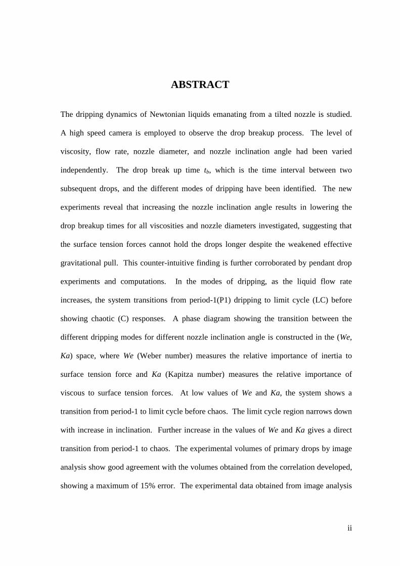
ABSTRACT

The dripping dynamics of Newtonian liquids emanating from a tilted nozzle is studied.

A high speed camera is employed to observe the drop breakup process. The level of

viscosity, flow rate, nozzle diameter, and nozzle inclination angle had been varied

independently. The drop break up time tb, which is the time interval between two

subsequent drops, and the different modes of dripping have been identified. The new

experiments reveal that increasing the nozzle inclination angle results in lowering the

drop breakup times for all viscosities and nozzle diameters investigated, suggesting that

the surface tension forces cannot hold the drops longer despite the weakened effective

gravitational pull. This counter-intuitive finding is further corroborated by pendant drop

experiments and computations. In the modes of dripping, as the liquid flow rate

increases, the system transitions from period-1(P1) dripping to limit cycle (LC) before

showing chaotic (C) responses. A phase diagram showing the transition between the

different dripping modes for different nozzle inclination angle is constructed in the (We,

Ka) space, where We (Weber number) measures the relative importance of inertia to

surface tension force and Ka (Kapitza number) measures the relative importance of

viscous to surface tension forces. At low values of We and Ka, the system shows a

transition from period-1 to limit cycle before chaos. The limit cycle region narrows down

with increase in inclination. Further increase in the values of We and Ka gives a direct

transition from period-1 to chaos. The experimental volumes of primary drops by image

analysis show good agreement with the volumes obtained from the correlation developed,

showing a maximum of 15% error. The experimental data obtained from image analysis

iii

further suggest that, in the P1 regime the pendant drop volume varies such that the trend

of the primary drop volume differs significantly from that of the breakup time.

iv

ABSTRAK

Dinamik penitisan cecair Newtonian berpunca daripada muncung condong dikaji. Sebuah

kamera berkelajuan tinggi digunakan untuk memerhatikan proses pemecahan titisan.

Tahap kelikatan, kadar aliran, diameter muncung, dan sudut muncung telah diubah secara

bebas. Penurunan masa pemechan tb, iaitu selang masa di antara dua titik yang berikutan,

dan pelbagai mod penitisan telah dikenalpasti. Ujikaji baru mendedahkan bahawa

peningkatan sudut muncung cenderung menurunkan selang masa perpecahan titisan untuk

semua kelikatan dan diameter muncung disiasat, seterusnya mencadangkan bahawa daya

ketegangan permukaan tidak boleh memegang titisan lebih lama walaupun tarikan graviti

berkesan yang lebih lemah. Penemuan lawan jangkaan ini disokong lagi oleh ujikaji

titisan tergantung bebas dan pengiraan. Dalam mod penitisan, dengan kenaikan kadar

aliran, sistem beralih dari kitaran-1 (P1) kepada kitaran terhad (LC) sebelum

menunjukkan gejala huru-hara (C). Gambar rajah fasa yang menunjukkan peralihan

antara mod penitisan yang berbeza untuk sudut muncung yang berbeza dibina dalam

ruang (We, Ka), di mana We (nombor Weber) mengukur kepentingan relatif inersia

kepada daya tegangan permukaan dan Ka (nombor Kapitza) mengukur kepentingan relatif

kelikatan ke daya ketegangan permukaan. Pada kadar aliran cecair yang rendah dan

kelikatan rendah, sistem ini menunjukkan peralihan daripada kitaran-1 kepada kitaran

terhad. Rejim kitaran terhad menjadi lebih sempit dengan peningkatan sudut muncung.

Peningkatan dalam nilai-nilai Ka dan We memberikan peralihan terus dari tempoh-1 ke

huru-hara. Isipadu titisan utama melalui analisis imej ujikaji menunjukkan persetujuan

yang baik dengan isipadu yang diperolehi daripada sekaitan yang dicadangkan, dengan

menunjukkan ralat maksimum 15%. Data ujikaji yang diperolehi daripada analisis imej

mencadangkan bahawa dalam rejim P1, isipadu titisan tergantung berubah sedemikian

sehingga pola isipadu titisan utama berbeza dengan ketara dengan masa perpisahan.

v

ACKNOWLEDGEMENT

I gratefully acknowledge my endless indebtedness to my supervisors Dr Yeoh Hak Koon

and Dr Pankaj Doshi (National Chemical Laboratory, Pune, India), without whose

guidance and support this thesis could not have been prepared.

Author likes to thank University for funding and excellent analytical facility, Dept. for

maintaining the instrument. The authors thank University of Malaya for sponsoring trip of

Dr. Pankaj Doshi to Malaysia. Acknowledgement is made to National Chemical

Laboratory for technical support in surface tension and rheology measurements. The

author is grateful to Mr. Krishnaroop Chaudhuri for the help in Surface Evolver setup.

Last but not the least; I thank my family and my friends for their continual support to

complete this work.

Place:

______________________

Dated: Amaraja Taur

Dept of Chemical Engineering

University of Malaya

vi

TABLE OF CONTENTS

Chapter Topic Page no

1 Introduction ........................................................................................................................ 1

1.1 Research Background .................................................................................................. 1

1.2 Motivation ................................................................................................................... 7

1.3 Objectives of Present Work......................................................................................... 9

1.4 Outline of the research approach ............................................................................... 10

2 Literature Review............................................................................................................. 11

2.1 History of Drop Formation ........................................................................................ 11

2.2 Drop formation dynamics.......................................................................................... 15

2.2.1 Primary drop formation...................................................................................... 15

2.2.2 Satellite drop formation ..................................................................................... 21

2.3 Effects of experimental parameters on drop formation ............................................. 27

2.3.1 Physical properties of the liquid ........................................................................ 27

2.3.2 Liquid rheology .................................................................................................. 30

2.3.3 Liquid flow rate.................................................................................................. 33

2.3.4 Nozzle geometry ................................................................................................ 35

2.3.5 Nozzle inclination .............................................................................................. 37

3 Research Methodology .................................................................................................... 38

3.1 Introduction ............................................................................................................... 38

3.2 Experimental setup .................................................................................................... 38

3.3 Fluid Characterization ............................................................................................... 39

3.4 Experimental procedure ............................................................................................ 41

3.5 Image Analysis Methods ........................................................................................... 42

3.5.1 Breakup Time Calculations................................................................................ 42

3.5.2 Primary Drop Volume Calculation .................................................................... 44

4 Results and Discussion .................................................................................................... 49

4.1 Dripping modes ......................................................................................................... 49

4.1.1 Time series analysis ........................................................................................... 52

4.1.2 Time return maps ............................................................................................... 60

4.2 Phase diagram ........................................................................................................... 63

vii

4.3 Effect of nozzle inclination on drop breakup time at low Weber number ................ 67

4.4 Interrogating the origin of the effect of the angle of tilt on tb ................................... 76

4.5 Volume of primary drops from image analysis ......................................................... 80

4.5.1 Comparison of drop volume obtained from correlation developed and from

image analysis .................................................................................................................. 80

4.5.2 Comparison of breakup time and drop volume with drop number .................... 83

5 Conclusion ....................................................................................................................... 97

Appendix A- MATLAB codes....................................................................................... 103

Appendix B- Experimental set-up images ..................................................................... 116

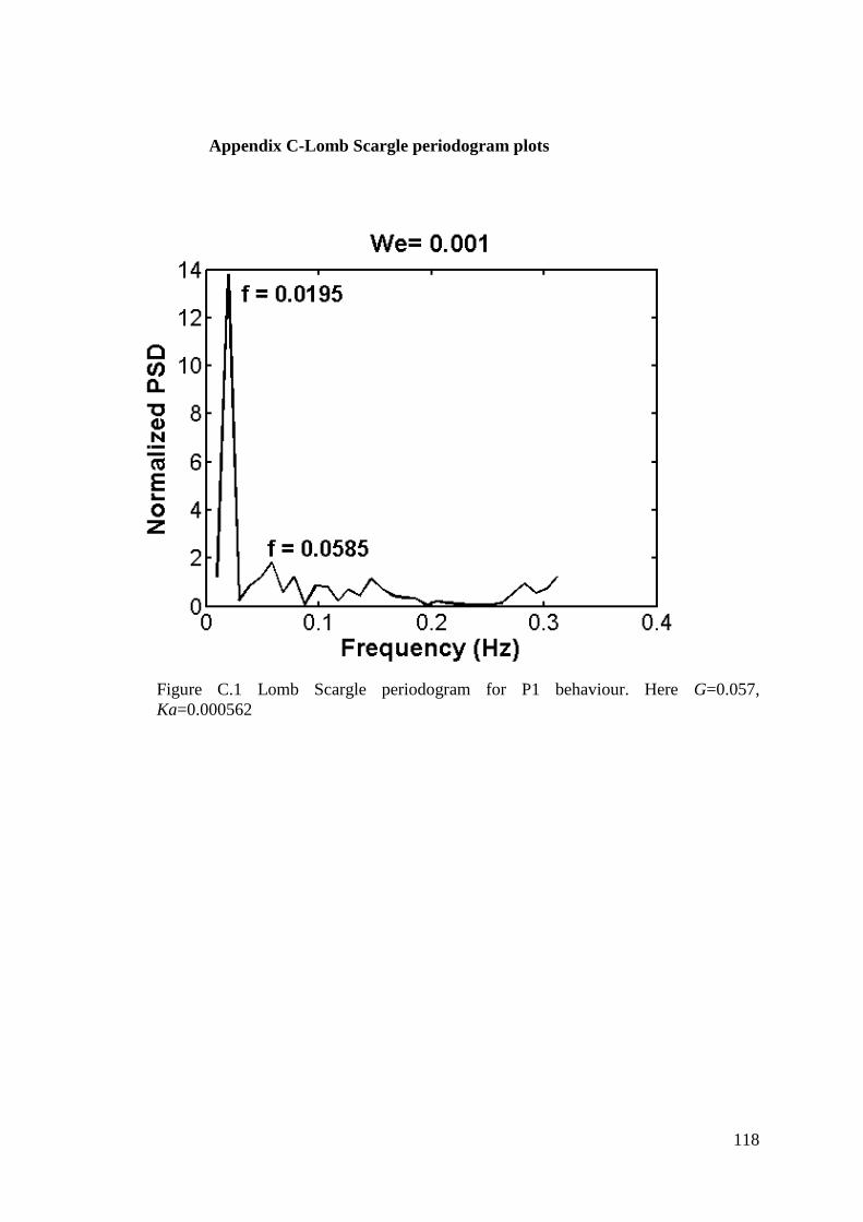
Appendix C-Lomb Scargle periodogram plots .............................................................. 118

Appendix D- List of Publications and Conferences Attended ....................................... 121

viii

LIST OF FIGURES

Figure No Title Page No

Figure 1.1 A dolphin in the New England Aquarium in Boston, Massachusetts; Edgerton

(1977). [Adapted from (Eggers, 1997)] ............................................................................... 2

Figure 1.2 Drop formation sequences showing primary and satellite drop. ........................ 4

Figure 1.3 Drop formation from a vertical nozzle. ............................................................. 6

Figure 2.1 Drop breakup process of a liquid jet 6 mm in diameter showing main drops

and satellite drops (Eggers, 2006). ..................................................................................... 11

Figure 2.2 Growing perturbations on a jet of water [adopted from (Eggers, 1997)] ......... 13

Figure 2.3 Secondary neck formations for water glycerol mixture (85%). (A) The

elongated liquid thread forms a secondary neck just above the primary drop (B) A

magnified region near breakup point (C) Same region as in (B), very near to breakup

process. ............................................................................................................................... 18

Figure 2.4 Drop shapes of water dripping from a nozzle of diameter 0.16 cm at the liquid

flow rate 1ml/min, taken at different time intervals (Zhang and Basaran, 1995). ............. 19

Figure 2.5 Computed shapes of drops, solid white curves, overlaid on experimentally

recorded images of identical drops of glycerine–water mixtures at near the drop breakup.

The viscosity of the liquid increases from left to right. ..................................................... 20

Figure 2.6 Breakup sequences of oil column suspended in a mixture of water and alcohol

(obtained from (Eggers, 2006)).The small perturbations grow on liquid cylinder which

grows giving minima and maxima on the liquid thread to result in to three small satellites

at each breakup. ................................................................................................................. 22

ix

Figure 2.7 A sequence of drop formation from a pipette, where both satellite and primary

drops are visible (Lenard 1887, obtained from ref (Eggers, 2006)). For the first time, the

sequence of events leading to satellite formation can be appreciated. .............................. 23

Figure 2.8 Typical sequences of drop formation for water and mixture of water glycerine.

............................................................................................................................................ 24

Figure 2.9 Stroboscopic microphotograph of liquid thread breaking at upper end of the

liquid jet (From Pimbley &Lee 1977.) .............................................................................. 25

Figure 2. 10 Shapes of liquid drop from a nozzle having diameter 1.5 mm close to break

up times for the liquids with increasing viscosity from A to E (Guthrie, 1863). The

liquids are water glycerol mixtures having viscosities 0.01 P (A), 0.1 P (B), 1 P (C), 2 P

(D), 12 P (E). ...................................................................................................................... 28

Figure 2. 11 Typical drop formation process for a neutrally buoyant suspension system

from a nozzle of diameter d=0.32 cm. The surrounding liquid is silicone oil and the

suspended particles has diameter d=212-250 µm. ............................................................. 31

Figure 2.12 Different regimes of drop formation, (a) Dripping with satellite formation,

(b) Dripping without satellite drop formation, (c) Jetting, The flow rates increases from

left to right (Scheele and Meister, 1968). .......................................................................... 34

Figure 3.1 Schematics of the experimental setup. ............................................................ 39

Figure 3.2 Image analysis of drop breakup process. Intensity value „1‟ represents black

part and „0‟ represents white part of the image. ................................................................. 43

Figure 3.3 Drop breakup sequences. The time interval between sequence (c) and (f) is the

breakup time tb. .................................................................................................................. 43

Figure 3.4 Experimental setup for vertical nozzle dripping experiments for volume

measurements ..................................................................................................................... 45

Figure 3.5 Volume measurement method for a axisymmetric drop .................................. 46

x

Figure 3.6 Experimental setup for vertical nozzle dripping experiments for volume

measurements ..................................................................................................................... 47

Figure 3.7 Images taken from two cameras kept at 90° to each other. .............................. 48

Figure 4.1 Variation of the dimensionless dripping time with drop number. Three

different dripping behaviours are seen as We increased, namely P1 ( We=0.05), LC

( We=0.15), and C ( We=0.30). Here G=0.057, Ka=0.000562 ..................................... 50

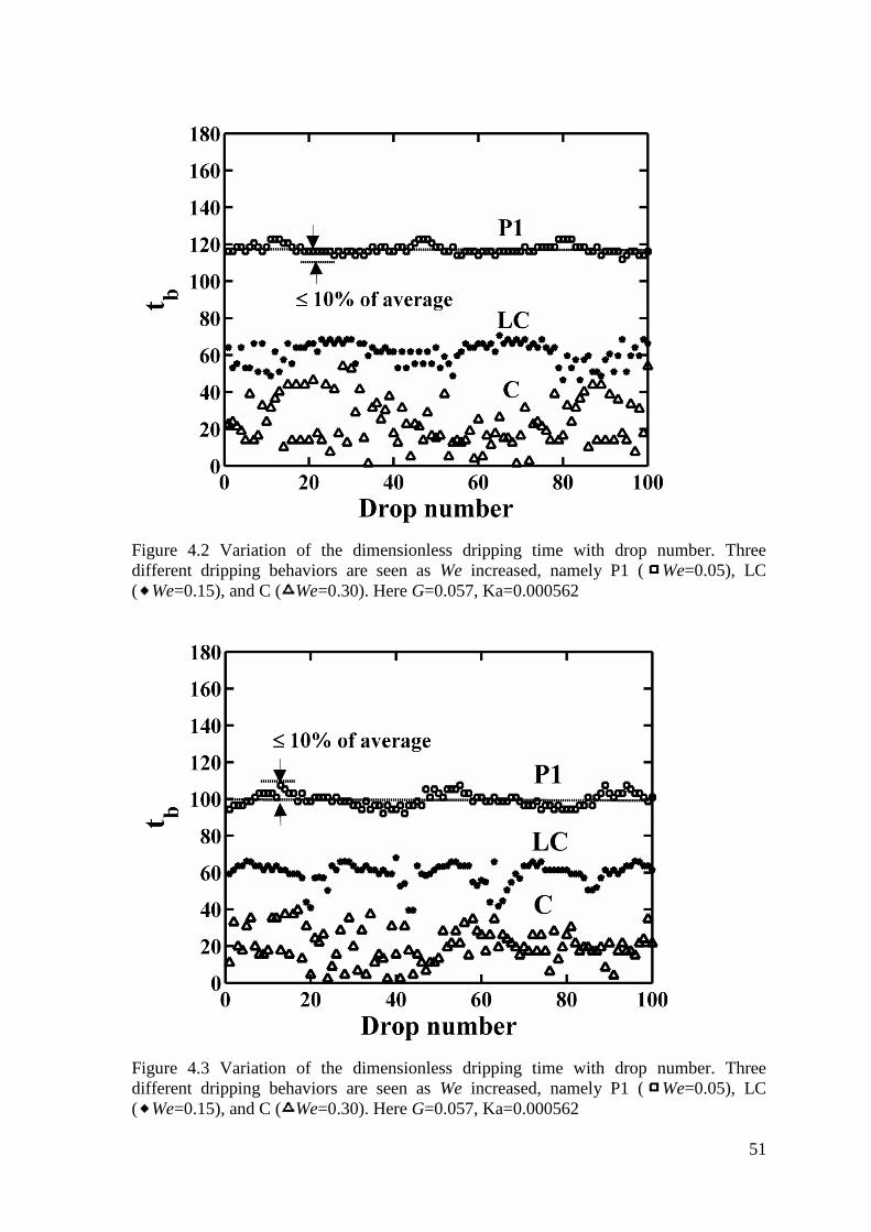
Figure 4.2 Variation of the dimensionless dripping time with drop number. Three

different dripping behaviours are seen as We increased, namely P1 ( We=0.05), LC

( We=0.15), and C ( We=0.30). Here G=0.057, Ka=0.000562 ..................................... 51

Figure 4.3 Variation of the dimensionless dripping time with drop number. Three

different dripping behaviours are seen as We increased, namely P1 ( We=0.05), LC

( We=0.15), and C ( We=0.30). Here G=0.057, Ka=0.000562 ..................................... 51

Figure 4.4 FFT plot for time data having P1 behaviour. Here We=0.05,G=0.057,

Ka=0.000562 ..................................................................................................................... 53

Figure 4.5 FFT plot for time data having LC behaviour. Here We=0.15,G=0.057,

Ka=0.000562 ..................................................................................................................... 54

Figure 4.6 FFT plot for time data having C behaviour. Here We=0.3,G=0.057,

Ka=0.000562 ..................................................................................................................... 54

Figure 4. 7 a Lomb Scargle periodogram for P1 behaviour. Here G=0.057, Ka=0.000562

........................................................................................................................................... 55

Figure 4.7 b Lomb Scargle periodogram for P1 behaviour. Here G=0.057, Ka=0.000562

........................................................................................................................................... 56

Figure 4.7 c Lomb Scargle periodogram for LC behaviour. Here G=0.057, Ka=0.000562

........................................................................................................................................... 56

xi

Figure 4.7 d Lomb Scargle periodogram for LC behaviour. Here G=0.057, Ka=0.000562

........................................................................................................................................... 57

Figure 4.7 e Lomb Scargle periodogram for C behaviour. Here G=0.057, Ka=0.000562 57

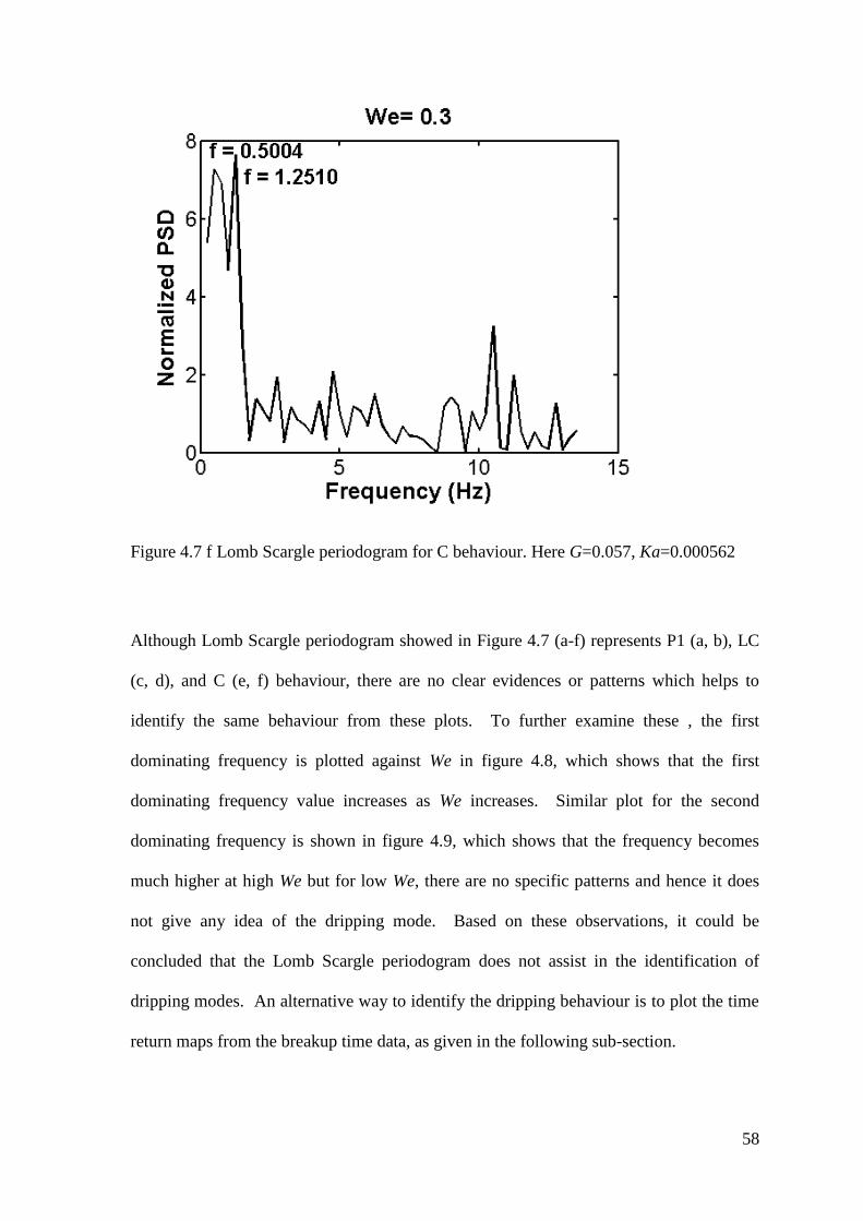
Figure 4.7 f Lomb Scargle periodogram for C behaviour. Here G=0.057, Ka=0.000562 58

Figure 4.8 First dominating frequency vs We obtained from Lomb Scargle periodogram.

........................................................................................................................................... 59

Figure 4.9 Second dominating frequency vs We obtained from Lomb Scargle

periodogram. ...................................................................................................................... 59

Figure 4.10 Time return maps showing P1 (a-f), LC (g-i), and C (j-k) behaviour. Here

G=0.057, Ka=0.000562. .................................................................................................... 62

Figure 4.11 An experimental phase diagram in (We, Ka) space at =0° (a), =30° (b),

=60° (c), showing transitional Weber numbers WeLC Wec. Here G=0.062. 66

Figure 4.12 Breakup time tb at different angle of inclination for P1 behaviour. The

experiments were performed at G=0.057, Ka=0.000562 and We=0.05. ........................... 68

Figure 4.13 Breakup time tb at different angle of inclination for LC behaviour. The

experiments were performed at G=0.057, Ka=0.000562 and We=0.15. ........................... 69

Figure 4.14 Breakup times as a function of Weber number. Here S0, S20 and S80

represent 0%, 20%, and 80% glycerol by weight respectively. N1 represents the nozzle

of OD 1.25 mm, and N3 is the largest nozzle of OD 3.92 mm. ........................................ 71

Figure 4.15 Predicted volume V vs experimental volume Vexp. The dashed lines

represent ±10% error in volume. Here 0.0005≤We≤0.1, 3.22×10-4

≤ Ka ≤ 5.26×10-2

and

=0°, 30°, 60°. ................................................................................................................... 75

Figure 4.16 Stable drop shapes pinned on a circular roof at different , side view, at

G=0.06. The roof is in the X-Y plane and gravity is acting along the vertical downward

direction. ............................................................................................................................ 78

xii

Figure 4.17 Experimental and computed variation of the dimensionless critical volume

Vc/Vo with . ...................................................................................................................... 79

Figure 4.18 Predicted volume V and image analysis volume Vimg change with We in P1

regime for θ=0˚ (a), θ=30˚ (b), θ=60˚ (c).The experiments were performed at G=0.057

and Ka=0.000562. ............................................................................................................. 82

Figure 4.19 a Comparison of drop breakup time tb and volume Vimg with drop number for

P1 mode. Here G=0.057, Ka=0.000562, and θ=0˚. ........................................................... 84

Figure 4.19 b Comparison of drop breakup time tb and volume Vimg change with drop

number for P1 mode. Here G=0.057, Ka=0.000562, and θ=0˚. ....................................... 85

Figure 4.19 c Comparison of drop breakup time tb and volume Vimg with drop number for

P1 mode. Here G=0.057, Ka=0.000562, and θ=0˚. .......................................................... 85

Figure 4.19 d Comparison of drop breakup time tb and volume Vimg with drop number for

P1 mode. Here G=0.057, Ka=0.000562, and θ=0˚. .......................................................... 86

Figure 4.19 e Comparison of drop breakup time tb and volume Vimg change with drop

number for P1 mode. Here G=0.057, Ka=0.000562, and θ=0˚. ....................................... 86

Figure 4.19 f Comparison of drop breakup time tb and volume Vimg with drop number for

P1 mode. Here G=0.057, Ka=0.000562, and θ=0˚. .......................................................... 87

Figure 4.20 a Comparison of drop breakup time tb and volume Vimg with drop number for

LC mode. Here G=0.057, Ka=0.000562, and θ=0˚. ......................................................... 88

Figure 4.20 b Comparison of drop breakup time tb and volume Vimg with drop number for

LC mode. Here G=0.057, Ka=0.000562, and θ=0˚. ......................................................... 88

Figure 4.20 c Comparison of drop breakup time tb and volume Vimg with drop number for

LC mode. Here G=0.057, Ka=0.000562, and θ=0˚. ......................................................... 89

Figure 4. 21 Comparison of drop breakup time tb and volume Vimg with drop number for

C mode. Here G=0.057, Ka=0.000562, and θ=0˚. ........................................................... 90

xiii

Figure 4.22 Comparison of drop breakup time tb and volume Vimg with drop number for

P1 mode (a), LC mode (b), and C mode (c). Here G=0.057, Ka=0.000562, for θ=30˚. .. 92

Figure 4.23 Comparison of drop breakup time tb and volume Vimg with drop number for

P1 mode (a), LC mode (b), and C mode (c). Here G=0.057, Ka=0.000562, for θ=60˚. .. 93

Figure 4.24 Comparison of pendant drop and primary drop volume ................................ 94

xiv

LIST OF TABLES

Table No Title Page No

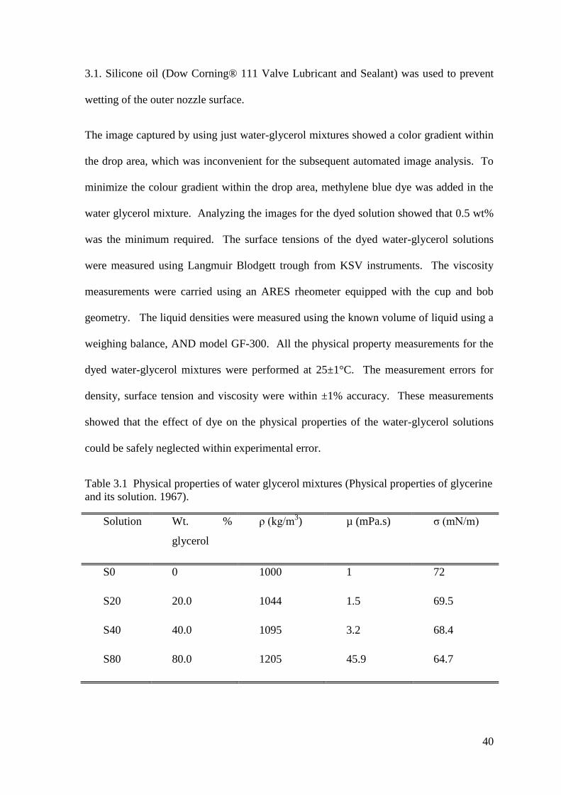
Table 3.1 Physical properties of water glycerol mixtures (Physical properties of glycerine

and its solution. 1967). ...................................................................................................... 40

Table 4.1 Magnitude of the slopes of the lines obtained from Fig. 4.14 ........................... 72

Table 4.2 Correlation function f values. ............................................................................ 94

xv

LIST OF SYMBOLS AND ABBREVIATIONS

Symbols

Roman alphabets

g Acceleration due to gravity

G Bond number

Ka Kapitza number

Q Liquid flow rate

R Radius of the nozzle

bt~ Drop breakup time

tb Dimensionless drop breakup time

v Velocity of the liquid

V~

Drop volume

V Dimensionless drop volume

We Weber number

Greek alphabets

θ Nozzle inclination angle from the vertical

ρ Density of the liquid

σ Surface tension of the liquid

Abbreviations

C Chaos

LC Limit cycle

P1 Period-1

SE Surface evolver

xvi

N1 Nozzle-1

N2 Nozzle-2

N3 Nozzle-3

S0 0% glycerol in water glycerol solution

S20 20% glycerol in water glycerol solution

S40 40% glycerol in water glycerol solution

S80 80% glycerol in water glycerol solution

1

1 Introduction

1.1 Research Background

Drop formation from a nozzle is phenomenon ubiquitous in nature and industries. The

phenomenon of drop breakup, drop collision, and drop formation involving free surface

flow is not only beautiful, but also is a challenging physical problem for researchers. The

drop formation process in the nature has been observed and the richness in the physics of

the drop formation has been identified which attracted the attention of scientist and

engineers over the years.

A drop may form when liquid accumulates at the lower end of a tube or other surface

boundary. Drop may also form by the condensation of a vapor or by atomization of a

larger mass of liquid. Rain drop formation is the best example of drop formation seen in

the nature, where the liquid droplets formed from the condensation of atmospheric water

vapor get precipitated, which later becomes heavy enough to fall under gravity. Another

example is the water in the form of small droplets that is generally seen on thin, exposed

surfaces in the morning or evening as a result of water vapor condensation called dew.

The large surface area of the exposed surface aids the radiation process cooling the

exposed surface which helps in the condensations of the atmospheric moisture, resulting

in the formation of droplets. The drop formation resulting from the dripping of water

from the roof and tap are also interesting examples which clearly show the individual

events of detaching drops.

The description of the flow and drop formation process shown in the Figure 1.1 would be

more complicated than one might think. Instead, it is much more useful to focus on the

2

individual events of drop formation, to gain some general insight into the dynamics which

can help to investigate the global behaviour of the process.

Figure 1.1 A dolphin in the New England Aquarium in Boston, Massachusetts; Edgerton

(1977). [Adapted from Eggers (1997)]

A simple way to form a drop is to allow liquid to flow slowly from the lower end of a

vertical nozzle of small diameter. The surface tension of the liquid tries to minimize

the liquid drop interfacial tension which allows the liquid volume to hang at the lower

end of the nozzle. This hanging drop is called pendant drop. Later the pendant drop

becomes unstable when drop volume exceeds a certain limit. The drop later detaches

under the influence of gravitation pull. The detached drop is called as primary drop

and the small drop volume produced during the detachment process which is

undesirable for industrial application is called satellite drop. This drop formation

process from a vertical nozzle has been an interesting area because of many industrial

3

applications such as ink-jet printing (Le, 1998), silicone microstructure array (Laurell

et al., 2001), emulsion formation (Sachs et al., 1994), 3D micro-printing (Walstra,

1993), microencapsulation etc (Freitas et al., 2005).

In most of the applications the most desired drop formation process should give

uniform size distribution and fast production rate. Even though the drops generically

results from the motion of free surfaces, it is not easy to predict their size distribution

and the dynamics involved in the process. The key parameters which controls this

drop formation process are physical properties of liquid, size and shape of nozzle,

liquid ejection velocity etc. The physical properties of the liquid consist of the surface

tension, density and viscosity of the liquid. Whereas the different shapes of nozzle

can be flat nozzle or obliquely cut nozzle. The slow drop formation can be observed

at very low liquid ejection velocity, whereas at high velocity the liquid can eject as a

column of the liquid which subsequently breaks into drops. The detailed studies of

the dynamics involved in the drop formation process were not possible before high-

speed digital cameras could be used for the photography in the experiments and

powerful computers for the simulations.

Drop formation thus results in an extremely broad spectrum of different droplet sizes.

The distribution of sizes was first time noticed 200 years ago by Felix Savart (1833)

in Paris. He observed that the water jet emanating from a small diameter orifice

separates in to tiny droplets in the span of perhaps a 1/100 th

of a second. Drop

formation sequences are shown in the Figure 1.2, where the jet of water is being

ejected from a vertical nozzle with primary and satellite drop formation. Generally

the formation of droplet is periodic in nature, but sometimes with primary drop, a

4

smaller "satellite" drop is seen as a result of drop breakup process. This satellite drop

formation is undesirable because they are far more readily misdirected by

aerodynamic and electrostatic forces and can thereby degrade the printing resolution.

Yet another example is the formation of satellite drops during crop spraying. The

lighter satellite drops of herbicides or pesticides are more easily transported to the site

other than that intended (spray drift). Beside waste and inefficiency spray drift from

pesticides and herbicide application exposes people and the environment to residues

that causes undesired health and environmental effects (Dravid, 2006).

Figure 1.2 Drop formation sequences showing primary and satellite drop.

Thus the arrival of ink-jet printing technology, that the consequences of Savart's

observations were fully appreciated. Ink-jet printing has been implemented in many

different designs and has a wide range of potential applications. Ink-jet is a non-

impact dot-matrix printing technology in which droplets of ink are jetted from a small

aperture directly on a targeted object on a specified media to create an image (Le,

1998). Thus the technical importance of the drop formation process and its

continuous study from last 300 years (Eggers, 1997) led to intense development in

ink-jet printing technology. For example, in the printing applications of integrated

circuits the ink is replaced by solder (Liu and Orme, 2001). In biotechnology,

thousands of DNA-filled water drops can be analyzed in parallel, by placing them in

Satellite drop

Primary drop

5

an array on a solid surface (Basaran, 2002). All these techniques rely on the

production of drops of well-controlled size, and satellite drops are highly detrimental

to the quality of the product.

Many liquid dosage forms in the pharmaceutical and biotech industries are based on

micro droplets (Kippax and Fracassi, 2003). The liquid pharmaceutical dosages in

aerosol form are directly sprayed on affected areas. The individual liquid drop sizes

and the amount of the liquid dosage sprayed on the affected area decide the amount of

drug absorbed, hence controlling these parameters becomes very important in the

pharmaceutical industries. The same efforts have been made to control the liquid

drop size distribution and their velocities in the agricultural sprays in order to increase

the efficiency (Lake, 1977).

Fundamentally the process of drop formation can be broken down in to dripping,

jetting and drop on demand. The first two methods occur under the action of gravity,

where dripping is the phenomenon of ejection of liquid from a nozzle to form droplets

when flow rate is sufficiently low, while jetting is phenomenon at high flow rates in

which liquid flows out as a continuous stream to form a jet which subsequently breaks

up in to small droplets. The third method i.e. drop on demand involves external

electrical force to control the drop formation process.

A Newtonian liquid having viscosity µ, density ρ, and surface tension σ, flowing

through a nozzle of radius R, at flow rate Q is the most commonly investigated

configuration for drop formation studies as shown in Figure 1.3. For a vertical nozzle

the dripping dynamics are governed by three dimensionless groups (Subramani et al.,

2006; and Basaran, 1995; Clasen et al., 2009): Weber number We= ρv2R/σ that

6

measures the relative importance of inertial to surface tension force, a Bond number

G= ρgR2/ σ, where g is the acceleration due to gravity, that measures the relative

importance of body force to surface tension force, and Kapitza number Ka= (µ4g/

ρσ3)1/3

or Ohnesorge number Oh=µ/(ρRσ)1/2

, both measures the relative importance of

viscous force to surface tension force.

Figure 1.3 Drop formation from a vertical nozzle.

The quantitative studies usually focus on the measurement of volumes of the liquid

droplets (Subramani et al., 2006), the liquid thread length before breakup (Zhang and

Basaran, 1995), and time interval between two drop breakups (Clasen et al., 2009).

7

1.2 Motivation

As addressed before the increased technological applications of drop formation

grabbed the attention of scientist to get enough inside in to the drop formation

process. Drop formation from a nozzle or an orifice has been the subject of numerous

theoretical and experimental studies (Eggers, 1997). Most of the attention to date has

focused on studies of the drop formation from a vertical nozzle, where the studies are

done either by changing the liquid properties or by changing the liquid flow rate

(Zhang and Basaran, 1995; Ambravaneswaran et al., 2000). In some of the studies the

effect of nozzle size and shape is also studied (Zhang and Basaran, 1995; D'Innocenzo

et al., 2004). Though the large number of studies shows that there has been enough

research done on the drop formation, but a lot is to be explored which is explained in

the paragraph below.

Despite the considerable amount of efforts devoted to droplet formation studies, there

has been a little attention directed towards drop formation studies from an inclined

nozzle. In this system, the nozzle is inclined at an angle θ and liquid is passed

through a nozzle to form small liquid droplets. The introduction of asymmetrical

perturbations, by tilting the nozzle at an angle (Reyes et al., 2002) breaks the

cylindrical symmetry and found strong changes in dripping dynamics when compared

with those obtained from a vertical nozzle. In the experiments on dripping from a

tilted nozzle, it is showed that the inclination angle can constitute an effective control

parameter by breaking the axis symmetry thus adding the asymmetric perturbations.

However, previous studies are far from being comprehensive, thus unable to provide

the proper explanations on the general behaviour of drop formation from a tilted

nozzle.

8

However, so far, there are no reports on the general behaviour of different modes of

drop formation from an inclined nozzle. The reported data only showed the strong

change in the dripping behaviour of an inclined nozzle even for small nozzle

inclination angle θ = 5° (Reyes et al., 2002). To this end it is highly desirable to know

the details about the general behaviour of drop formation from an inclined nozzle.

9

1.3 Objectives of Present Work

In this work, focus will be given on the drop formation study from an inclined nozzle

and the results will be compared with its behaviour when nozzle is in vertical position.

Some of the results will be further highlighted and compared with the computations.

As the details about the general behaviour of drop formation process from an inclined

nozzle is not provided before, the results obtained in this work will provide useful

information. The main objectives of this work are summarized as follow:

a) To investigate the different dripping modes by investigating the drop breakup time

tb, for different and We values. The different modes of dripping are shown on

the phase diagrams which are constructed in (We, Ka) space for all G and

values. The effect of on the formation of satellite drops is also highlighted in

the phase diagram.

b) To investigate the effect of We, Ka, G and on the dripping time tb. This

finding was summarized in a correlation for the dimensionless breakup volume V

over wide ranges of G, Ka and .

c) To investigate the breakup volumes of the drop from tilted nozzle dripping

experiments using image analysis.

10

1.4 Outline of the research approach

In Chapter 2, a literature review is presented. A brief history of drop formation study

presented followed by detailed review with their key findings and recent development in

same area is given.

In Chapter 3, a brief introduction about the methodology is provided followed by the

experimental setup with the fluid characterization and properties. In the same chapter the

experimental procedure is given followed by details on image analysis method and

breakup time calculations.

In Chapter 4, results on different dripping modes for both vertical and inclined nozzle are

presented and also the modes of dripping are shown on phase diagrams. The effect of

on drop breakup time in the P1 regime are presented for a wide range of parameters and

results obtained on the same are corroborated with some experiments and computer

simulations which later gives a correlation for drop breakup volume. The breakup

volumes of primary drops by image analysis also compared with that obtained from the

correlation developed.

The conclusions are given in chapter 5.

11

2 Literature Review

2.1 History of Drop Formation

Early experiments of Savart ( 1833) demonstrated that the liquid jet flowing out from

nozzle first decays in to small undulations and then droplets. Savart illuminated the

liquid jet as shown in Figure 2.1 by using a light source. He simply assumed liquid jet as

a circular cylinder and observed that the tiny undulations grow on liquid jet. These

undulations then grow large enough and results in to droplets. Without photography, it

was very difficult to make experimental observations, since the time scale at which the

drop breakup occurs is very small. Yet Savart was able to extract a remarkably accurate

and complete picture of the actual breakup process using his naked eye alone. The

observations on drop breakup process are well summarized in Figure 2.2 (Eggers, 2006).

To the left side of the figure, one sees a continuous jet of the liquid near the exit of

nozzle. Growing perturbations are seen next to the continuous jet until the point labelled

as „a‟, where drops start breaking up. The elongated liquid thread near „a‟ later becomes

part of the droplet. Both primary and tiny satellite drops are visible in the figure. The

fast moments involved in the drop formation process were not clearly resolved in the

figure.

Figure 2.1 Drop breakup process of a liquid jet 6 mm in diameter showing main drops

and satellite drops (Eggers, 2006).

12

Some of the Savart‟s observations are summarized as: (i) the liquid jet breakup is

independent of direction of gravity, physical properties of liquid, the diameter of liquid jet

and jet velocity; (ii) the tiny undulations always results from the perturbations received by

the liquid jet from the nozzle tip when it emanates from nozzle. Savart assumed that the

drop formation process involves balance between inertial and gravity force.

A few years later Plateau ( 1843) discovered that it‟s surface tension which causes liquid

jet perturbations to reduce its surface area by collecting the liquid in to one sphere in

order to maintain smallest surface to volume ratio. Identification of the surface tension

force was missing in Savart‟s study, however he made a reference to mutual attraction of

molecules which prefers to form a sphere of the liquid, around which the oscillations take

place. But the crucial role of the surface tension was identified by Plateau only. With

this results it follows as well whether the perturbations imposed on the liquid jet will

grow or not. The perturbations that will undergo reduction of surface area favored by

surface tension, and will thus grow.

Following up on Plateau‟s insight, Rayleigh (Rayleigh, 1879, Rayleigh and Strutt, 1879)

in 1879 studied the linear stability of liquid jet, where he noticed that, the surface tension

has to work against inertia, which opposes fluid motion over long distance. Rayleigh

assumed an infinitely long, initially stationary, circular, inviscid liquid jet of radius r and

the calculation made by this linear stability analysis allowed him to describe the initial

growth of instabilities as they initiate near the nozzle and continuous length of jet.

Rayleigh found that there is an optimal wavelength λ= 9r at which perturbations grow

faster, and which sets the typical size of drops. Rayleigh confirmed his theory within 3%

with the data Savart got 50 years before.

13

Figure 2.2 Growing perturbations on a jet of water [adopted from (Eggers, 1997)]

14

In the second half of the 19th

, many researchers had focus on the surface tension related

phenomenon, whereas different parameters affecting on drop dynamics was studied in

20th

century both experimentally and theoretically.

15

2.2 Drop formation dynamics

When the flow rate is small, a pendant drop hanging at the nozzle tip can detach when a

critical volume is reached resulting into primary drop. A small volume of liquid drop can

also results in the process of drop breakup giving satellite drop. Conceptually, drop

formation process can be divided into two stages: The first one corresponds to the growth

of the liquid at the end of the nozzle tip and second one corresponds to the necking and

breaking of the drop which may form only primary drop or both primary or satellite drop

depending upon the experimental parameters. A static description of the droplet breakup

patterns, neck formation, shape and size of the droplets are useful in the study and given

in the following subsections.

2.2.1 Primary drop formation

Historically, research on the drop formation was motivated mostly by engineering

applications, hence the liquid drop shape and a size has given more attention in the study.

When liquid is released slowly through a vertical nozzle, initially the surface tension

forces are in balance with the gravitational force. When inertia does not play any role,

one can easily see that the hanging drop goes through a sequence of equilibrium shapes.

These sequences of liquid drops are carefully studied by Worthington in 1881

(Worthington, 1881). Worthington noticed that, in the previous dripping experiments

carried by Guthrie (1863), the drop sizes were calculated based on the weight of the

droplets. But this study lacks the most important information of the liquid drops i.e.

shape and size of the droplet when it falls and goes thrugh the number of sequences.A

simple experimental technique allowed Worthington to observe the drop sequences, but

the observations are made without photographic technique hence the results were not

quantitative in nature.

16

The first quantitative experiments were done by Haenlein (1931) in 1931 using different

liquids having different densities, surface tension, viscosities, jet diameters and jet

velocities. The liquids tested were water, gas oil, glycerine and castor oil. A simple

apparatus was used to produce the liquid jet of 0.1 to 1 mm diameter with velocities

ranging from 2 to 70 m/s. The observations were made by using shadow pictures by

means of electric spark. Haenlein observed the disintegration time for different kinds of

liquid jets, where he found different patterns of disintegration of liquid jet: drop formation

without air influence, drop formation with air influence, formation of waves, and

complete disintegration of jet. These were the primary dripping experiments where the

primary drops were quantitatively observed for different experimental parameters. A step

ahead, Ohnesorge (McKinley and Renardy, 2011) used sophisticated spark flash timing

and variable exposure system, where the quality of the images and temporal resolution

was improved. The liquids of different physical properties were ejected from the nozzle

at different flow rates. Four important regimes were observed in the drop breakup

process in his experiments namely: Slow dripping, breakup of cylindrical jet by

axisymmetric perturbations, breakup by skew like perturbations, and atomization of jet.

Takahashi and Kitamura (1969) also carried out the dripping and jetting experiments on

liquids like water, kerosine, and glycerine surrounded air and immicible liquid and he

observed that the break up pattern in both the system are analogous to each other.

Takahashi observed that as the ejection velocity increased all the liquids shows dripping,

laminar jetting, and turbulant flow patterns.

A fascinating demonstration of Shi and Brenner (Shi et al., 1994) by experiments and

computations, using the one dimensional equation developed by Eggers and DuPont

(1994), that liquid thread or liquid neck can spawn a series of smaller necks with even

17

thinner diameters was a very important contribution in the study of secondary necks. In

the study, the different shapes of hanging drops for different liquid viscosities close to

drop breakup were focused, where they observed the dramatic change in primary drop

shape for different viscosities. As the value of viscosity increases the neck of the liquid

drop elongates and forms structure that is not seen in case of pure water. They observed

some secondary neck formations at the break up points for high viscosity liquids which

occurs by initial thinning near the drop followed by rapid extension of the neck upward

away from the drop as shown in the figure 2.3 (a-c). As the liquid neck becomes

sufficiently thin, it undergoes finite amplitude instabilities may be due to the thermal

noise. As a result of this, a secondary neck grows on a primary neck having self-similar

form. These observations were experimentally possible by high speed photography

where they could see the multiple stages of necking process before actual break up.

Simulation results on the same also shows that the near the bottom of the long neck there

is a region where the thickness of the neck decreases forming a secondary neck.

18

Figure 2.3 Secondary neck formations for water glycerol mixture (85%). (A) The

elongated liquid thread forms a secondary neck just above the primary drop (B) A

magnified region near breakup point (C) Same region as in (B), very near to breakup

process (Shi et al., 1994).

A detailed experimetal study by Zang and Basaran (1995) investigated the effect of all

relevant parameters on the drop breakup length for first time in the study. Figure 2.4

shows the evolution of liquid thread connecting the main drop and the remaining liquid

for water. It is very clear from the figure that during necking the portion of main drop

19

takes spherical shape and the remaining liquid thread looks like a liquid cone. Later the

liquid thread thins, and at certain neck diameter it detaches from the spherical drop which

later oscillates in vertical direction by changing its shape as seen in Figure 2.3 (l, m).

However the braking process can result in to formation of satellite drop as seen in Figure

2.3(m). Comparisons of the primary drop breakup volume measured in the experiments

are compared with predicted volume obtained from the empirical model of Scheele and

Meister (1968). The volumes measured experimentally are smaller than the predicted and

more deviation is seen at higher flow rates with maximum relative deviation of 25%,

showing relatively good agreement between experimental and predicted volume. In same

study Zhang and Basaran obtained a detailed phase diagram for different viscosity, flow

rate and nozzle radius. The phase diagram details about main drop, satellite drop size and

neck length.

Figure 2.4 Drop shapes of water dripping from a nozzle of diameter 0.16 cm at the liquid

flow rate 1ml/min, taken at different time intervals (Zhang and Basaran, 1995).

The predictions of the computations made by Wilkes et al. (1999) made by using a 3D,

axisymmetric or 2D finite element algorithm have been shown to agree with couple of per

20

cent with the experimental results which confirms the high degree of accuracy in the

calculations. The volumes of the drops are found to mostly affected by the interplay

between gravity and surface tension force. The computed shapes of the drop are overlaid

on experimental shapes of the drops showing a very good agreement in figure 2.5. In the

same study, the algorithm developed is used for calculating limiting length and primary

drop volume for a wide range of parameter space spanned by relevant dimensionless

group.

Figure 2.5 Computed shapes of drops, solid white curves, overlaid on experimentally

recorded images of identical drops of glycerine–water mixtures at near the drop breakup.

The viscosity of the liquid increases from left to right (Wilkes et al., 1999).

21

2.2.2 Satellite drop formation

In the drop formation process, the primary drop does not form alone in some cases, a

undesirable form of a small drop volume also results in the breakup process called

“satellite drop”. These satellite drops actually decay the printing quality, as drop of

different size are deflected differently by an electric field. Hence understanding the cause

of satellite drop formation and possible control has been attracted the attention of

researchers in the field of drop formation.

The satellite drop formation was first observed by Savart in 1833 (Eggers, 2006). Figure

2.1 given in the above sub section 2.1, shows that the small satellite drops in between two

primary drops results during the liquid jet breakup. Later Plateau (1849) also included

some experimental sketches as shown in the figure 2.6 for oil suspended in to water

alcohol mixture. The nonlinear dynamics of drop liquid jet breakup of a viscous liquid

first goes through the elongation of the liquid thread and then tiny perturbations grows

forming minima at many places. The final stage of the breakup includes the formation of

primary and satellite droplets where he observed that the satellite drop is not alone formed

at the center of two primary drop, but also even smaller satellite drops are formed at right

and left of the satellite drop which indicates that the final stage of the breakup is much

more complicated that one would think. Without photography and with air as media

surrounding the drop, it was very difficult to observe the existence of the satellite drops in

the dripping experiments. Having these difficulties did not escape the attentive eyes of

Guthrie (Guthrie, 1863) in satellite drop observation. The kind of drops he observed were

the one which moves upward once they formed as a result of pinch off process.

22

Figure 2.6 Breakup sequences of oil column suspended in a mixture of water and alcohol

(obtained from (Eggers, 2006)).The small perturbations grow on liquid cylinder which

grows giving minima and maxima on the liquid thread to result in to three small satellites

at each breakup.

The stroboscopic method used by Lenard (1887) enabled him to take an entire sequence

to see the dynamics near the drop breakup with the time resolution that would otherwise

be impossible to achieve. These sequences first time showed the appreciable results for

satellite drop formation. In the satellite drop formation: first liquid neck breaks near to

the primary drop, but before it snap back it also thins near the pendant drop which later

breaks forming the satellite drop. These sequences are shown in the figure 2.7.

23

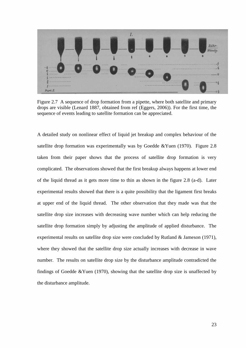
Figure 2.7 A sequence of drop formation from a pipette, where both satellite and primary

drops are visible (Lenard 1887, obtained from ref (Eggers, 2006)). For the first time, the

sequence of events leading to satellite formation can be appreciated.

A detailed study on nonlinear effect of liquid jet breakup and complex behaviour of the

satellite drop formation was experimentally was by Goedde &Yuen (1970). Figure 2.8

taken from their paper shows that the process of satellite drop formation is very

complicated. The observations showed that the first breakup always happens at lower end

of the liquid thread as it gets more time to thin as shown in the figure 2.8 (a-d). Later

experimental results showed that there is a quite possibility that the ligament first breaks

at upper end of the liquid thread. The other observation that they made was that the

satellite drop size increases with decreasing wave number which can help reducing the

satellite drop formation simply by adjusting the amplitude of applied disturbance. The

experimental results on satellite drop size were concluded by Rutland & Jameson (1971),

where they showed that the satellite drop size actually increases with decrease in wave

number. The results on satellite drop size by the disturbance amplitude contradicted the

findings of Goedde &Yuen (1970), showing that the satellite drop size is unaffected by

the disturbance amplitude.

24

Figure 2.8 Typical sequences of drop formation for water and glycerine (Goedde and

Yuen, 1970).

A new experimental results on satellite drop breakup revealed that the liquid thread may

break at upper side of ligament first, lowers side of ligament side or simultaneously at

both the end (Pimbley and Lee, 1977). The best example of ligament breaking first at

upper side of the liquid thread is shown in the figure 2.9, taken from their paper. Another

observation they made was that the satellite drop may merge forward or backward

25

depending upon the disturbance amplitude. If the satellite is formed by breakup of liquid

thread due to breakup at both the ends simultaneously then the satellite drop speed

remains equal to the speed of primary drop and this condition of breakup is called

“infinite satellite condition”.

This is the first reported experimental observation that contradicts the observations made

by Goedde and Yuen (1970) that the liquid thread always breaks at lower end in the

satellite drop formation process.

Figure 2.9 Stroboscopic microphotograph of liquid thread breaking at upper end of the

liquid jet (From Pimbley & Lee, 1977.)

In the later part of the twentieth century, the effects of different experimental parameters

like nozzle dimensions, flow rate, rheological properties, and physical properties of the

liquid on the satellite and primary drop formation was investigated. The next subtopic

26

gives the literature review on the effect of these parameters on the drop formation

dynamics.

27

2.3 Effects of experimental parameters on drop formation

2.3.1 Physical properties of the liquid

The physical properties of the liquids like viscosity, surface tension, and density can have

some effect on the drop formation dynamics. As the viscosity of the liquid is varied, the

changes in liquid drop shape were investigated both experimentally and computationally

(Shi et al., 1994). Figure 2.10 shows photographic events of the shape and length of the

liquid length change near the drop breakup for different viscosities. The viscosity of the

liquid increases from A-E in figure 2.10, where A and E represents pure water and pure

glycerol respectively. By mixing the water with glycerol, the viscosity of the liquid can

be varied by 103 times and the surface tension was not varied more than 15% so that the

effect of viscosity was more visible. As seen in the figure 2.10, the liquid thread length

increases as the viscosity of the liquid increases from A-E. Also they observed that, as

the value of viscosity increases the neck of the liquid drop elongates and forms structure

that is not seen in case of pure water. Another distinct feature observed for high viscosity

liquid drop, as discussed earlier, the high viscosity liquid shows secondary neck

formations at the break up points which occurs by initial thinning near the drop followed

by rapid extension of the neck upward away from the drop. The simulation results

obtained for drop shapes were found to be very similar to the photographic events

obtained near the drop breakup.

Building on the previous findings of Shi et al. (1994), Zhang and Basaran (1995)

demonstrate the important role played by viscosity on the necking and drop breakup

dynamics of the forming drop. Aside from the noticeable difference in the size of the

28

drop near to the drop breakup, Zhang and Basaran demonstrate the variation of

dimensionless drop

Figure 2. 10 Shapes of liquid drop from a nozzle having diameter 1.5 mm close to break

up times for the liquids with increasing viscosity from A to E (Guthrie, 1863). The

liquids are water glycerol mixtures having viscosities 0.01 P (A), 0.1 P (B), 1 P (C), 2 P

(D), 12 P (E).

29

elongation i. e. neck length with relative time for pure water and 85% water glycerol

mixture. In the same study the drop volumes and neck lengths for 20%, 50%, 70%, and

80% water glycerol solutions are investigated. Viscosity plays a very important role in

stabilizing the grooving drop which makes possible larger drop elongation by damping

and it eliminating the interfacial oscillations, but has virtually no effect on drop size. The

finding here on the drop stabilizing due to viscosity has found to have two important

aspects in the drop formation. First, viscosity promotes the damping of interfacial

oscillations remained on pendant due to the breakup of previous drop and second, the

viscosity keeps the about to fall primary drop nearly spherical in shape. These

observations are important in the area of polymer beads formation, where the drop

sphericity has a prime importance.

Zhang and Basaran (1995) in the same study investigated the effect of surface active

agent on the drop formation dynamics. By just adding different concentration of the

surface active agent like triton, can change the surface tension of the liquid by keeping

density and viscosity of the liquid virtually constant. So the role played by surface

tension in the dynamics of the drop formation was easily identified. The drop breakup

volume of the pure water and 0.01 and 0.05 % triton solution is compared. The results

accords well with the intuition that at low flow rate the breakup volume of primary drops

decrease with increase in surfactant concentration. Consequently, because of the

reduction in the volume of the primary drops, the limiting length also decreases with

increase in surfactant concentration. The similar experiments are performed for the high

flow rates and the surface dilation occurs at high rate giving increasing primary drop

breakup volume and breakup length values as surfactant concentration increases. The

volumes of satellite drops also compared in the same study. The volume of satellite drops

found to increase with increase in surfactant concentration. The well-known facts about

30

the surfactant are that the surfactant greatly damp and suppress the surface waves

stabilizing the growing and stretching liquid thread. This leads to increase in the liquid

volume of a thread and hence satellite drop volume.

2.3.2 Liquid rheology

Rheology of the liquid may complicate the drop formation, when it is compared to its

Newtonian counterparts. The rheology of the fluid can be changed by addition of micron

size particles to the Newtonian liquid. Furbank and Morris (2004) studied the particles

effect on drop formation, where the particles used were in micron size suspended in

viscous liquid. The density of particles and the surrounding liquid was matched to make

the system neutrally buoyant so that one can neglect the settling effect. The suspensions

were investigated for different volume fractions and dripping experiments were

performed for three different nozzle sizes. The typical drop formation process for a

neutrally buoyant suspension system from a nozzle is shown in the Figure 2.11. The

dripping behaviour for low volume fraction ɸ shows the similar behaviour as that of pure

liquid, but at high volume fraction ɸ the dripping behaviour is markedly different. The

addition of particles in the liquid suppress the number of satellite drop formation at higher

volume fraction, but few satellite drops were still noticed having size much larger than in

pure liquids. The dripping to jetting transition was observed at small flow rate for a fine

value of volume fraction, but at high volume fraction ɸ the transition becomes less abrupt

and difficult to identify.

31

Figure 2. 11 Typical drop formation process for a neutrally buoyant suspension system

from a nozzle of diameter d=0.32 cm. The surrounding liquid is silicone oil and the

suspended particles has diameter d=212-250 µm (Furbank and Morris, 2004).

Cooper-White et al.(2002) investigated the effect of liquid elasticity on dripping

dynamics, where two types of fluids having similar viscosity,density, and surface tension

but different elasticity were studied for dripping experiments. The results showed similar

behaviour till the formation of lower pinch region for all types of liquids regardless of

elasticity, which gives proper justification for importance of capillary and inertial forces

before lower pinch occures. But once the lower pinch is occurred, the break up time for

elastic liquid is increased compared to Newtonian liquid. This break up time increases

with increase in fluid elasticity. Later in 2008 Li and Sundararaj (2008) studied the

breakup mechanism for viscoelastic liquid drop. They found that the drop size of a

viscoelastic fluid determines the drop breakup mechanism and also the critical point

where the mechanism changes. The small drops break in the direction which is

perpendicular to the flow direction and large drops break along the flow direction.

32

Breakup of capillary jet of dilute polymer solution showing gobbling phenomenon which

is the result of the dynamic interaction of capillary breakup in a falling viscoelastic jet

with a large terminal drop that serves as a sink for the mass and momentum of the

incoming fluid is studied. The gobbling phenomenon which is observed near the

transition from dripping to jetting and the thinning process of the ligament connecting the

main drop and pendant drop for a viscoelastic polymer solution is explained (Clasen et

al., 2009). The high speed photography technique used to observe the gobbling

phenomena showed that the gobbling is actually a form of delayed dripping process and

the thinning process of the ligaments that are subjected to a constant axial force is driven

by surface tension and resisted by the viscoelasticity of the dissolved polymeric

molecules.

The later work of Clasen et al. (2011) focus on the dispensing behaviour of rheologically

complex fluids and its behaviour is compared with their Newtonian counterparts.The

properties of liquid that they varied are fluid viscosity, elsticity, and the degree of shear

thinning. The drop break up mechanism, drop volumes, and break up times have been

observed using high-speed video-microscopy. To predict the thinning and dispensing

behaviour of rheologically complex fluids, different nondimensional groups which

defines the relative importance of different forces involved, that is, the Ohnesorge, elasto-

capillary number, and Deborah number have been defined. With the different values of

these nondimensional numbers in the experiments one can to identify the dominant

mechanism resisting breakup and its corresponding critical dimensionless number. These

critical values also allow one to identify the filament life times. German and Bertola

(2010) experimentally investigated the formation and detachment of liquid drops from a

capillary nozzle for Newtonian fluids of variable viscosity, shear-thinning fluids, and

viscoplastic or yield-stress fluids. The experimental results showed that the behaviour of

33

Newtonian and shear-thinning drops is qualitatively similar, and leads to the formation of

spherical drops, viscoplastic drops exhibit strongly prolate shapes and a significantly

different breakup dynamics of the capillary filament.

2.3.3 Liquid flow rate

The complexity in the dripping behaviour can be seen by increasing the flow rate of the

dispensing liquid. The different modes of dripping seen in the experiments include

period-1 dripping where every drop is of equal size, period-n (n=2,3,4…..) dripping

where every n-th drop is identical, and higher odd-period or chaotic mode of dripping

(Subramani et al., 2006; Zhang and Basaran, 1995; Clasen et al., 2009; Ambravaneswaran

et al., 2000; Scheele and Meister, 1968; Wilkes et al., 1999). Wilkes et al. (1999) studied

low viscosity Newtonian fluids at low flow rate, where the dripping behaviour changes

from Period-1 to some complex dripping, chaotic responses and then at high flow rates

the transition takes place from complex dripping to jetting. But high viscosity liquids

shows direct transition from simple dripping to jetting as flow rate increases.

Ambravaneswaran et al. (2004) investigated this transition at different flow rates and at

different viscosities. For constant viscosity and constant nozzle size, the different

regimes of drop formation are explained in Figure 2.12 where the flow rate is increasing

from left to right. At low flow rate the dripping with satellite drop formation is observed

and with increasing flow rate the observed region is the dripping region without satellite

drop formation (Figure 2.12 (b)) which can be simply a Period-1 or complex dripping or

chaotic behaviour. Further increase in flow rate gives jetting behaviour in the system

where the droplets detach from the end of long liquid thread as shown in Figure 2.12 (c).

In the same study, phase diagrams were constructed in (We, Ka) space shows the

34

transition between different modes of dripping. As an extension of this work, the critical

We for transitions from one mode to another were estimated by scaling arguments and

shown to accord well with simulations (Subramani et al., 2006). Initially the phase

diagram developed in (We, Oh) space was constructed for a moderate value of G=0.5

(Subramani et al., 2006), but the reponse if the value of G varies was unknown. This

unexplored dripping dynamics for a wider range of G was later studied by Subramani et

al. (2006). It was found that at high values of G, the dripping dynamics is richer and

tends to become chaotic at lower values of We. In the same study they found that, at very

low flow rates, a tiny satellite drop often follows the primary drop. If the viscosity of the

dispensing liquid is increased (high Oh), the dripping behaviour simplifies to either P1

with satellites or jetting (Subramani et al., 2006). A detailed phase diagram showing

transitions from complex to simple dripping and jetting in the (We, Oh) space had been

reported (Subramani et al., 2006).

Figure 2.12 Different regimes of drop formation, (a) Dripping with satellite formation,

(b) Dripping without satellite drop formation, (c) Jetting, The flow rates increases from

left to right (Scheele and Meister, 1968).

35

2.3.4 Nozzle geometry

If the liquid wets the entire thickness of the nozzle, the radius of the contact circle equals

the outer radius of the nozzle in all the experiments. Even if R is considered as a radius

of contact circle, it is important to know the effect of ratio Ri/R (where Ri is the inner

radius of the nozzle) on the drop formation dynamics. The variation of drop volume and

drop breakup length with Ri/R is investigated by keeping flow rate and viscosity constant

(Zhang and Basaran, 1995). As ratio Ri/R decreases i.e. as the thickness of the nozzle

increases, the elongation of drop at drop breakup increases giving increased length of the

liquid thread and hence the drop breakup volume decreases. The further decrease in the

ratio Ri/R diminishes the effect of wall thickness on drop volumes and liquid thread

length at some critical value of Ri/R>0.2. At this critical value, the drop volumes, liquid

thread length and even the shapes of the liquid drops are found within experimental error

to be identical to those obtained when the nozzle has virtually zero thickness. This

finding helps to choose the proper nozzle in the experiments where one can simply

neglect the effect of wall thickness.

The critical role of nozzle geometry was investigated by changing the two parameters in

the experiments: first the inner nozzle diameter and second the nozzle shape

(D‟Innocenzo et al., 2002). The dripping dynamics found to be almost similar for

relatively large values of the inner nozzle width. In addition, radical changes in the

dripping dynamics were found when the nozzle shape changes from a flat tip to a

bevelled shape. Dripping dynamics of relatively narrow internal diameter changes

considerably for different nozzle shapes. In particular, the observation shows that the

inner diameter can have a control parameter to change the dripping dynamics of the

nozzle. A very useful finding on nozzle thickness showed that, the wall dimension of the

36

nozzle influences substantially the dripping behaviour, for the nozzles with a ratio of

thickness of the wall to inner radius ≤ 0.2. The satellite drop formation for beveled tips

nozzle is found to be notable reduced. As an extension of this work a detailed study on

the effect of different nozzle geometry on dripping behaviour is done by D‟Innocenzo et

al. (2004). Two types of nozzle geometries, flat and obliquely shaped cut tip nozzle he

considered for dripping experiments. For same flow rate and viscosity the dripping

behaviour for these two different nozzles is compared. The obtained result shows the

dramatic change in the dripping behaviour when nozzle shape changes from flat to

obliquely cut shape. They found that the added degree of freedom produces a transversal

oscillation of a pending drop, which couples with a vertical oscillation which is the result

of the break off of the previous drop. As a result of that the dripping times are found to

be shortened and dripping patterns are more regularize. This results into the decreased

frequency of the vertical oscillations of the residue and reduced contact circle. They

observed a very complex liquid flow patterns and eddies of different amount. The

frequency of drop oscillations decreased going from the flat nozzle tip to the bevelled

nozzle tip and to the obliquely cut nozzle (D‟Innocenzo et al., 2004). It was claimed that

this was due to wetting characteristics of the liquid with the wall of the nozzle as it

determines three phase contact line affecting the dripping time series behaviour

(D‟Innocenzo et al., 2004).

37

2.3.5 Nozzle inclination

The introduction of asymmetrical perturbations, by tilting the nozzle at an angle with

the vertical breaks the cylindrical symmetry and induced strong changes in dripping

dynamics (Reyes et al., 2002). The topological considerations to characterize heteroclinic

scenario uniquely from the time series of the dripping faucet experiment are used to

investigate the influence of the nozzle inclination, representing symmetry breaking in the

system, and generating heteroclinic tangle. In the experiments on dripping from a tilted

nozzle, the measured time (Tn) between the nth

and (n+1)th drop were plotted, giving time

return maps for different nozzle inclination angle . The obtained time return maps

showed that even for small inclination angle =5°, the system symmetry breaks and

dripping behaviour changes dramatically. The results showed strong changes in the

attractor topology, suggesting that inclination angle can be an effective control parameter

for the dripping dynamics (Reyes et al., 2002).

Despite the rich dynamics of dripping from a tilted nozzle, we failed to uncover any other

articles in the English literature. Due to the limited range of parameters studied

previously (Reyes et al., 2002), the more general behaviour of dripping from a tilted

nozzle remains unknown. The main goal of this paper is to develop a comprehensive

picture of the dripping dynamics from a tilted nozzle. In order to achieve that goal, (a)

dripping dynamics will be explored through the study of the breakup time bt , which is the

time interval between two subsequent drop breakups, and (b) dripping phase diagrams for

different values of will be constructed.

38

3 Research Methodology

3.1 Introduction

The experiments are designed to obtain the quantitative information on the drop breakup

time and the drop breakup volume. Attention is also paid in the experiments to the

satellite drop formation for different experimental conditions. The experiments are

performed by varying liquid viscosity, flow rate, nozzle size, and nozzle inclination angle.

3.2 Experimental setup

The experimental setup is depicted in figure 3.1. It consists of a nozzle through which

liquid flows to form drops. The liquid was delivered to the nozzle by using a

MeditechJZB-1800D Syringe Pump which is capable of providing range of flow rate

from 0.00167 to 30 mL/min with an accuracy of ±2%. Stainless steel dispensing nozzles

(P-30619-06, P-30619-01, and P-30619-07) were obtained from Cole-Parmer. The outer

radii of the nozzles are 0.625 mm (N1), 1.00 mm (N2), and 1.96 mm (N3). The ratio of

the inner radius to outer radius is <0.2, hence the effect of nozzle thickness on the

interface dynamics can be safely neglected (Zhang and Basaran, 1995). A protractor is

provided to adjust the tilt angle of the nozzle. A transparent shield is provided to reduce

draft that can perturb the drop formation process.

The high speed camera is Casio EX-FH100 capable of recording 30 to1000 frames per

second. A planar white LED backlight measuring 10 cm 10 cm (model LFL-Si100-W-

IP65) with adjustable brightness was obtained from Falcon Illumination (M) Pte. Ltd.

The sharpness of the images can be adjusted via the intensity of the backlight, the focal

39

length and digital zoom of the camera. All parts of apparatus except the syringe pump

were kept on a 0.3m×0.3m×0.06m aluminium optical base plate inside the transparent

shield.

Figure 3.1 Schematics of the experimental setup.

3.3 Fluid Characterization

Mixtures of water and glycerol were chosen because their surface tension and densities

are almost similar to that of pure water, but their viscosities can be made to vary three

orders of magnitude. The 99% pure glycerol obtained from R and M Chemicals, CAS

NO [56-81-5], and used as obtained. Distilled water was used to the make water glycerol

mixtures. The physical properties of these water glycerol mixtures are taken from the

literature (Physical properties of glycerine and its solution. 1967) and are listed in Table

40

3.1. Silicone oil (Dow Corning® 111 Valve Lubricant and Sealant) was used to prevent

wetting of the outer nozzle surface.

The image captured by using just water-glycerol mixtures showed a color gradient within

the drop area, which was inconvenient for the subsequent automated image analysis. To

minimize the colour gradient within the drop area, methylene blue dye was added in the

water glycerol mixture. Analyzing the images for the dyed solution showed that 0.5 wt%

was the minimum required. The surface tensions of the dyed water-glycerol solutions

were measured using Langmuir Blodgett trough from KSV instruments. The viscosity

measurements were carried using an ARES rheometer equipped with the cup and bob

geometry. The liquid densities were measured using the known volume of liquid using a

weighing balance, AND model GF-300. All the physical property measurements for the

dyed water-glycerol mixtures were performed at 25±1°C. The measurement errors for

density, surface tension and viscosity were within ±1% accuracy. These measurements

showed that the effect of dye on the physical properties of the water-glycerol solutions

could be safely neglected within experimental error.

Table 3.1 Physical properties of water glycerol mixtures (Physical properties of glycerine

and its solution. 1967).

Solution Wt. %

glycerol

ρ (kg/m3) µ (mPa.s) σ (mN/m)

S0

S20

S40

S80

0

20.0

40.0

80.0

1000

1044

1095

1205

1

1.5

3.2

45.9

72

69.5

68.4

64.7

41

3.4 Experimental procedure

The experimental run began with applying a thin layer of silicone oil on the outer wall of

the nozzle. This pinned the liquid to the outer sharp edge of the nozzle tip even at

inclined positions. The verticality of the nozzle was checked with two perpendicularly

mounted pendulums. Following this, the tilt angle was adjusted using a protractor. The

prepared solution was drawn into the syringe and any bubble present in the syringe or

tube was purged off. A desired flow rate was then set on the syringe pump. The drop

formation sequences were recorded at 240-420 frames per second depending upon the

liquid flow rate. The recorded videos were first converted into images with the ImageJ

software (ImageJ software, retrieved on 10 August 2012), then analyzed using an

algorithm written in MATLABTM

software to detect the drop breakup and to calculate the

breakup time between two successive drops.

In this work, the experiments were performed at different values of We (5×10-4

to 0.45)

by varying the liquid flow rate Q, Ka (3.22×10-4

to 0.0526) by changing the viscosity µ of

the liquid, G (0.053 to 0.70) by using three different nozzle radius R, and (0°, 30°, and

60°). All the experiments were carried out at room temperature (25±1°C).

42

3.5 Image Analysis Methods

3.5.1 Breakup Time Calculations

The images so retrieved are analyzed using an algorithm written in MATLAB (Appendix

A.1) software to detect the drop breakup and to calculate the breakup time tb between two

successive drops. The MATLAB algorithm takes the images of a set of experiments.

These images are first read in to the MATLAB, which are later converted in to black and

white (BW) images. MATLAB reads these images in three dimensional matrix forms,

where each pixel value in the corresponding direction is assigned to the row and columns

of the matrix. The images we have are the two dimensional images, which has the pixel

values in „x‟ and „y‟ direction only, which assigns these values in column vector and row

vector of the matrix respectively, and the third dimension of the matrix is always kept

constant. Once the images are converted in to BW image, there are only two different

pixel values, that is „1‟ and „0‟ as shown in Figure 3.2 (b), where pixel value „1‟

corresponds to the dark part of the image and „0‟ corresponds to the bright part of the

image. We have intensity threshold, which has to be given before we convert a RGB

image to BW image. Deciding the value of intensity threshold is very important in the

process as it decides the part of the image which has to consider as black or white, hence

it needs some trial and error experiments. Once the images are converted in to BW form,

the drop break up is detected on the basis of intensity difference near nozzle area. If the

intensity difference values are changed from 1-1-1 (Figure 3.2 (a)) to 1-0-1 (Figure 3.2

(b)), then the very first image is detected as drop breakup image.

43

(a) (b)

Figure 3.2 Image analysis of drop breakup process. Intensity value „1‟ represents black

part and „0‟ represents white part of the image.

Some of the sequences of drop formation from a vertical nozzle are shown in the Figure

3.3, where the image sequence (c) and (f) represents the drop breakup instant and hence

drop breakup image on the basis of intensity difference criteria explained in the previous

paragraph. Once the drop breakup image numbers are detected, the breakup time tb is

calculated on the basis of image number and frame rate of the camera. The time interval

between these two image sequences ((c) and (f)) represents the drop breakup time tb.

.… ….. …. …. ….

(a) (b) (c) (d) (e) (f)

Figure 3.3 Drop breakup sequences. The time interval between sequence (c) and (f) is the

breakup time tb (Resolution: 0.21 mm/pixel).

1

1

0

1

1

1

44

3.5.2 Primary Drop Volume Calculation

3.5.2.1 For the Vertical Nozzle

The volumes of primary drops are also measured using the same images obtained for the

tb calculations using a MATLAB code (Appendix A.2). For the experiments from a

vertical nozzle, the liquid drop is symmetric in shape. So the images of the liquid drops

from one fixed angle using just one camera are taken as shown in Figure 3.4. The drop

breakup images initially detected were further sent to MATLAB for volume calculation.

These images are initially converted in to BW format and value of one pixel is initially

calculated by the dimensions of a reference object (In our experiments the nozzle

diameter was the reference dimension to convert pixels into centimeters). To measure the

drop volume for each image, initially we assumed each drop as a symmetric shape akin to

an ellipsoid. The drop is then divided in two vertical sections along the major axis as

shown in figure 3.5. Each vertical section has „n‟ number of radius equal to the number

of pixels on a vertical axis. The radius is measured by calculating the number of pixels

on a horizontal line representing a radius at a particular location. The different radii are

shown in figure 3.5. At the same position, the value of the radius used for volume

calculations is the average values for two radii. By using combined Simpsons 1/3 rd and

3/8 th rule for numerical integration over the entire asymmetric shape, the volume for a

drop from one angle is calculated. For the same experiments, the error in the

measurement is calculated by weighing 10 drops from the similar experiments. The

average weight of the 10 drops (14 mg) was then converted to volume via the density of

the water-glycerol solution. The error between the weighed drop volumes and volumes

obtained from image analysis was within 3%.

45

Figure 3.4 Experimental setup for vertical nozzle dripping experiments for volume

measurements

46

Figure 3.5 Volume measurement method for a axisymmetric drop

3.5.2.2 For an Inclined Nozzle

In the experiments of dripping from a inclined nozzle, the images of drop sequences are

taken from two angles placed at 90° to each other so that even if the drop is asymmetric in

shape, we can measure the drop diameters from two different angles to have more

accurate estimates of the volumes of the drops. These two drop breakup images taken

from two different angles are detected and sent to the MATLAB programme (Appendix

A.2) for volume calculations. The method of volume calculation is similar to the method

mentioned above for vertical nozzle, but for inclined nozzle experiments there are two

images at same instant. Though these two images are taken from two different angles as

shown in figure 3.6, the major axis of the asymmetric drop shape is a vertical axis which

is clearly understood in figure 3.7 snapshots taken for similar drops from two different

angles. As vertical axis is common in both the images, the two images can be easily

47

correlated for the volume calculations. These two images are analyzed the same way

mentioned above and the average volume of these two images is taken to be the volume

of asymmetric drop. The volumes obtained from the image analysis for asymmetric drops

was verified with the volume calculated from a drop weighing method and found to be

within a maximum of 5% error.

Figure 3.6 Experimental setup for vertical nozzle dripping experiments for volume

measurements.

48

Figure 3.7 Images taken from two cameras kept at 90° to each other.

Angle-1 Angle-2

49

4 Results and Discussion

In the section below, the different modes of dripping for a vertical nozzle are identified on

the basis of drop breakup times and their evaluation with total time. Some other

approaches to identify the dripping modes are also given. Similarly the dripping modes

for different are identified and a phase diagram for each value in (We, Ka) space is

given in the following section. In the next section, a similar phase diagram showing the

effect of on satellite drop formation is constructed. Later the effect of on dripping

time is also shown section followed by the computational approach to confirm the

obtained results. The drop volume measurements for primary drops and its comparison

with drop breakup time is given in the following sub section.

4.1 Dripping modes

Experiments with a vertically oriented nozzle illustrate the various dripping modes

observed. The breakup time, bt was made dimensionless using capillary time

3R .

Throughout the remainder of this report, a variable with a tilde designates a dimensional

variable while one without denotes the dimensionless counterpart of the same variable.

Fig. 4.1 shows the variation of the dimensionless breakup time tb, with drop numbers. As

depicted in Fig. 4.1, values of tb decreases with increase in Weber number. Based on this,

three different dripping regimes were encountered, namely period-1 (P1), limit cycle

(LC), and chaos (C). At low Weber numbers, every droplet had the same tb value, and

this mode was denoted as the period-1 dripping (P1). At moderate Weber numbers, the tb

50

trajectory repeated itself, showing low amplitude and low frequency oscillations around

the average. This was denoted as the limit cycle (LC) behaviour. The chaotic (C)

behaviour was seen at high Weber numbers, where the tb trajectory did not repeat itself,

showing disorderly long term evolution.

Figure 4.1 Variation of the dimensionless dripping time with drop number. Three

different dripping behaviors are seen as We increased, namely P1 ( We=0.05), LC

( We=0.15), and C ( We=0.30). Here G=0.057, Ka=0.000562

51

Figure 4.2 Variation of the dimensionless dripping time with drop number. Three

different dripping behaviors are seen as We increased, namely P1 ( We=0.05), LC

( We=0.15), and C ( We=0.30). Here G=0.057, Ka=0.000562

Figure 4.3 Variation of the dimensionless dripping time with drop number. Three

different dripping behaviors are seen as We increased, namely P1 ( We=0.05), LC

( We=0.15), and C ( We=0.30). Here G=0.057, Ka=0.000562

52

Raising the angle of tilt to = 30oand 60

o, at constant We, Ka, and G, the evolution of tb

with drop number and the time return map is shown in Fig.4.2 and 4.3 respectively. The

features remain qualitatively identical. This is notable as the extent of asymmetry in the

liquid meniscus is significant at this inclination. It suggests that inclination probably

exerts higher order effects on the dripping dynamics. Nevertheless, comparing Figs. 4.1

and 4.3, the values of tb for the P1 regime decrease noticeably with an increase in ,

whereas the values for tb for the LC and the C modes of dripping are relatively

independent of . Since the flow rate remains identical, the droplets formed from the

inclined nozzle in the P1 regime must be smaller than their counterparts in the vertical

case. This opens up another avenue to regulate drop volumes.

The breakup time data obtained here for different experimental parameters can be

analyzed in different ways to identify the dripping behaviour. Some of the efforts made

to analyze the same are given in subsections below.

4.1.1 Time series analysis

To extract more meaningful statistical results from the data of drop breakup time, the time

series analysis is used. This is the first ever attempt made to identify the nature of the

phenomenon represented by the sequence of observations. In the time series analysis,

MATLAB algorithm for Fast Fourier Transform (FFT) (Appendix A.3) to compute the

Discrete Fourier Transform (DFT) is used to convert time data to frequency. The FFT

allows us to look at the data in frequency domain rather than in the time domain

(Bloomfield, 2004). The converted frequency domains are analyzed here to find out the

dominant frequency that may be present in the data and the patterns obtained may allow

53

us to identify and decide more efficiently the modes of dripping. If the obtained plots

shows any patterns, one can easily predict whether the time series obtained in dripping

experiments are of periodic nature (P-n, where n=1,2,….n) or chaotic in nature.

Following three FFT plots for time data are for P1, LC, and C behaviour respectively.

Figure 4.4 FFT plot for time data having P1 behaviour. Here We=0.05,G=0.057,

Ka=0.000562

54

Figure 4.5 FFT plot for time data having LC behaviour. Here We=0.15,G=0.057,

Ka=0.000562

Figure 4.6 FFT plot for time data having C behaviour. Here We=0.3,G=0.057,

Ka=0.000562

55

The FFT plots for P1, LC, and C time series data shown in figure 4.4, 4.5, and 4.6

respectively shows one dominant frequency peak. For P1 and LC plot, the plot has two

sub frequency peaks. The plots clearly do not show the frequency patterns to identify the

modes of dripping.

The data points for breakup time data are not equally spaced. So the more accurate FFT

method for non-equally spaced data points is Lomb Scargle method (Ruf, 1999) which

estimates a frequency spectrum based on a least squares fit of sinusoid called power

spectral density (PSD) normalized over frequency. A MATLAB algorithm is used to

obtain the periodogram for the same method (lomb.m file Appendix A.4). The plots

given in Figure 4.7 (a-f) shows the Lomb Scargle periodogram for P1 (a, b), LC (c, d),

and C (e, f) behaviour respectively.

Figure 4. 7 a Lomb Scargle periodogram for P1 behaviour. Here G=0.057, Ka=0.000562

56

Figure 4.7 b Lomb Scargle periodogram for P1 behaviour. Here G=0.057, Ka=0.000562

Figure 4.7 c Lomb Scargle periodogram for LC behaviour. Here G=0.057, Ka=0.000562

57

Figure 4.7 d Lomb Scargle periodogram for LC behaviour. Here G=0.057, Ka=0.000562

Figure 4.7 e Lomb Scargle periodogram for C behaviour. Here G=0.057, Ka=0.000562

58

Figure 4.7 f Lomb Scargle periodogram for C behaviour. Here G=0.057, Ka=0.000562

Although Lomb Scargle periodogram showed in Figure 4.7 (a-f) represents P1 (a, b), LC

(c, d), and C (e, f) behaviour, there are no clear evidences or patterns which helps to

identify the same behaviour from these plots. To further examine these , the first

dominating frequency is plotted against We in figure 4.8, which shows that the first

dominating frequency value increases as We increases. Similar plot for the second

dominating frequency is shown in figure 4.9, which shows that the frequency becomes

much higher at high We but for low We, there are no specific patterns and hence it does

not give any idea of the dripping mode. Based on these observations, it could be

concluded that the Lomb Scargle periodogram does not assist in the identification of

dripping modes. An alternative way to identify the dripping behaviour is to plot the time

return maps from the breakup time data, as given in the following sub-section.

59

Figure 4.8 First dominating frequency vs We obtained from Lomb Scargle periodogram.

Figure 4.9 Second dominating frequency vs We obtained from Lomb Scargle

periodogram.

60

4.1.2 Time return maps

The time return maps are the plots of time tn vs. tn+1, where nature of the plot helps to

investigate the periodicity of the time series data. Each point on the time return map is

determined by the ordered pair (tn, tn+1) for some n value. Previous researchers (Shaw,

1984; k Martien et al., 1985; D'Innocenzo and Renna, 1996, Subramani et al., 2006) have

used the time return maps to identify the structures and patterns from the simple plot to

define the dripping behaviour. The time return map responses for the same data given in

Figure 4.7 (a-f) are given below figure 4.10 for different modes of dripping.

(a) (b)

61

(c) (d)

(e) (f)

(g) (h)

62

(i) (j)

(k)

Figure 4.10 Time return maps showing P1 (a-f), LC (g-i), and C (j-k) behaviour. Here

G=0.057, Ka=0.000562.

The time return maps have shown in the figure 4.10 (a-k), represent the trajectories of

periodic orbits. In figure 4.10 (a-f), all the points are clustered together, ideally forming

only one point, represents the P1 behaviour. The spread between the data points is within

±10% of the average for P1 regime. For the limit cycle regime, the spread between the

data points is more than 10% of average value, but the trajectories repeat itself giving an

encircled regime on time return map as shown in figure 4.10 (g-i). At high Weber

63

number, the points are scattered rather randomly giving C mode of dripping as shown in

figure 4.10 (j-k).

The time return maps are shown to give good predictions about the modes of dripping,

hence are used in the investigation of modes of dripping for rest of the experimental data.

To facilitate discussions, the transition from P1 to LC is deemed to occur at We =WeLC,

and the transition from LC to C occurs at We =Wec. These two Weber numbers can be

pin-pointed experimentally. As the value of Ka changes, the corresponding values of

WeLC and Wec also change. The loci of these transitional We are plotted against Ka as a

dripping mode phase diagram next.

4.2 Phase diagram

The phase diagrams shown in figure.4.11 (a)-(c) identify the location in the parameter

space where the dynamics changes from one mode to another. For a vertical nozzle

(figure 4.11 a), at low values of Ka, both WeLC and Wec rise sharply as the value of Ka

increases. For high values of Ka, the trajectories of WeLC and Wec converge, i.e. the

transition occurs directly from P1 to C without exhibiting a LC regime. This is known as

the “simple dripping” region in the computational phase diagram of Subramani et al.

(Subramani et al., 2006) when G=0.3. Noting that Ka=(Oh4G)

1/3, their corresponding

value of Ka for such “simple dripping” regime is 0.67, nearly an order of magnitude

larger than ours. Further, in their work, the P1 region narrows down prior to the “simple

dripping” regime, whereas ours do not exhibit this narrowing. Certainly, keeping the P1

region wide at high values of Ka avails greater flexibility for applications. These

64

differences in the phase diagram highlight the very considerable effect of the value of G

on the dripping dynamics, also illustrated by the same authors.

The phase diagrams for an inclined nozzle look similar to that of the vertical nozzle.

However, on closer examination, three significant and potentially useful features can be

distilled. First, the values of Wec decrease dramatically with especially for Ka ~ 10-3

,

suggesting that the asymmetry favors chaotic dripping. This is in line with the findings of

Reyes et al. (Reyes et al., 2002), which showed that even at = 5o, the dripping dynamics

for low viscosity water turns very complicated. Second, the locus of WeLC is not so

strongly affected by at low values of Ka. It suggests that P1 and LC regimes are

influenced more by viscous damping than by asymmetry. A consequence of these two

observations is that the LC regime shrinks noticeably with increase in . Conceivably at

even larger values of , the LC region might vanish. However, we could not pursue that

in our experiments as the liquid started to wet the outer wall of the nozzle at large

inclinations despite the use of a dewetting agent.

At high values of Ka, however, the interaction of asymmetry with strong viscous damping

raises the values of WeLC, leading to the third observation: The values of We for direct

transition from P1 to C increase with . This avails an operating option to move the

chaotic dripping of a very viscous liquid into the well-defined P1 region simply by tilting

the nozzle. The modest increase in the values of this direction transition We against the

corresponding values for the vertical nozzle suggest that the effect of is most likely a

higher order effect and thus difficult to deduce from scaling arguments, as was done for

the jetting transition (Subramani et al., 2006).

65

66

Figure 4.11 An experimental phase diagram in (We, Ka) space at =0° (a), =30° (b),

=60° (c), showing transitional Weber numbers WeLC Wec. Here G=0.062.

67

4.3 Effect of nozzle inclination on drop breakup time at low Weber

number

Further insight into the dripping dynamics of an inclined nozzle can be gained by

examining the drop breakup times tb for different nozzle inclination angle . As shown in

figure 4.12, the value of tb at a given We decreases with increasing . As discussed

earlier, the tb values are unaffected by in the LC regime, but the number of repeating

trajectories for the LC regime at a given total time decreases with increase in as shown

in figure 4.13. The observation in figure 4.12 was further investigated at other values of

We, as represented by closed symbols in figure 4.14 (a). Clearly the values of tb decrease

with increasing when G=0.053. As the tb values in figure 4.14 are the average values

with a maximum of 10% spread (the value of spread decreases with increase in

viscosity), it is critical to determine if two sets of data at different angles were indeed

statistically different. Assuringly, using the Student‟s t-test, the probability of having

indistinguishable values of tb (as the angle changed) is very low (p value approximately

10-8

). Analogous behaviour is found even at ten times greater value of G (G=0.52) shown

by open symbols in figure 4.14 (b) as well as for different viscosities of the liquids, as in

figure 4.14 (c) and (d). In short, tb decreases with increasing for all values of G, We,

and Ka investigated.

68

Figure 4.12 Breakup time tb at different angle of inclination for P1 behaviour. The

experiments were performed at G=0.057, Ka=0.000562 and We=0.05.

69

Figure 4.13 Breakup time tb at different angle of inclination for LC behaviour. The

experiments were performed at G=0.057, Ka=0.000562 and We=0.15.

70

71

Figure 4.14 Breakup times as a function of Weber number. Here S0, S20 and S80

represent 0% (a, b), 20% (c), and 80% (d) glycerol by weight respectively. N1 represents

the nozzle of OD 1.25 mm, and N3 is the largest nozzle of OD 3.92 mm.

72

Table 4.1 Magnitude of the slopes of the lines obtained from Fig. 4.14

0° 30° 60° G

S0N1 0.5 0.5 0.5 0.053

S20N1 0.5 0.5 0.5 0.057

S80N1 0.5 0.5 0.5 0.071

S0N2 0.5 0.5 0.4 0.52

S20N2 0.5 0.5 0.4 0.56

S80N2 0.4 0.4 0.4 0.70

Figure 4.14 suggests that m

bt We . To examine the variability of the values of the slope

-m due to the 10% scatter inherent in the data points (representing averages), two lines

representing the worst-case scenario were drawn as follows: first a line connecting the

minimum (-10%) tb at the lowest We and the maximum (+10%) tb at the highest We;

second a line connecting the maximum (+10%) tb at the lowest We with the minimum (-

10%) tb at the highest We. The magnitudes of slopes for such two lines for each

experimental set are in between 0.4 and 0.6, suggesting that the values of the slopes in

figure 4.14 are accurate to the first significant digit only. Recognizing this observation,

Table 4.1 collects the magnitudes of the slopes for all the lines in figure 4.14. Most of

the values are approximately 0.5, suggesting

73

0.5

1bt

We (4.1)

Equation (4.1) leads to a rather counter-intuitive finding. It can be rewritten in the

dimensional form as, 1

btv

, where v is the velocity of the emanating fluid.

Rearranging and multiplying both sides by the internal cross sectional area A of the

nozzle results in bAvt AK , where K is the proportionality constant dependent on G, Ka

and . The left hand side is approximately the volume V of the detached liquid droplet;

this approximation is very good when the volume of pendant drop does not change

significantly. Random sampling of the recorded images suggested that this assumption is

very reasonable. This relationship offers a startling conclusion that the detached drop

volume in P1 dripping is rather independent of the flow rate. It also avails a very

convenient route to obtain the experimental drop volumes without analyzing the

complicated asymmetric drop images.

To compactly quantify this finding, by making V dimensionless with the volume of an

equivalent sphere based on the outer nozzle radius R, a power law correlation was tested:

32 4

1V (cos )cc c

c G Ka (4.2)

The choice of cosine of was mainly suggested by the component of gravity along the

axis of the nozzle. A nonlinear least squares regression of Eq. (4.2) using all data points

in the P1 regime yielded the coefficients:

74

1 0.02 0.37V 1.3 (cos )G Ka (4.3)

The dimensionless volumes V of the liquid droplets predicted are within 10% of

experiments, as plotted in figure 4.15. A similar regression analysis that included We

gave a very small (0.009) exponent for We, without any significant improvement in the

accuracy of predictions, further justifying its omission in Eq. (4.3). It is noteworthy that

figure 4.14 covers the widest ranges of parameters than previously reported, with up to

60o, Ka spanning three orders of magnitude and G one order of magnitude. Eq. (4.3) is

also significant as the first ever correlation for the droplet volume for P1 dripping from a

tilted nozzle. Further, it includes dripping from a vertical nozzle as a special case, valid

beyond vanishingly small values of Weber number (unlike the correlation in Yildirim et

al.) (Yildirim et al., 2005). It also shows that the 1/G dependence as hinted in figure 7 of

Ambravaneswaran et al. (Wilkes et al., 1999) remains valid for dripping from a tilted

nozzle.

75

Figure 4.15 Predicted volume V vs experimental volume Vexp. The dashed lines represent

±10% error in volume. Here 0.0005≤We≤0.1, 3.22×10-4

≤ Ka ≤ 5.26×10-2

and =0°, 30°,

60°.

76

4.4 Interrogating the origin of the effect of the angle of tilt on tb

As the angle of inclination increases, the component of gravity along the axis of the

nozzle decreases. Intuitively this should result in a decrease in the driving force for drop

formation as the gravitational pull on the emanating liquid has been weakened. At low

flow rates in which the inertial force is not dominating, surface tension forces should then

resist drop detachment for a longer time, giving an increased value of the breakup time tb,

and hence an increased drop volume. In contradiction, the experimental results showed

that the tb values decreased with increasing . This suggests that despite the weaker axial

component of gravity, the surface tension force is being weakened even more by the

asymmetric air-liquid interface. To probe the detailed interplay between these forces will

require a full 3-dimensional unsteady state simulation of the free surface motion which is

out of the scope of this work. In lieu of this, an alternative approach was pursued as

described below.

A pendant drop, which is pinned to the end of a nozzle, assumes a stable shape as long as

the drop volume is below a critical value, beyond that it becomes unstable leading to its

deformation and eventual breakup. At low Weber numbers typical of P1 dripping, the

key forces remain gravity and surface tension, whether the nozzle is tilted or not. Inertial

forces come into play only in the necking of the droplet in the last moments (Wilkes et

al., 1999), often comprising just a small fraction of the overall breakup time. This

similarity suggests that the drop formation process in slow P1 dripping is closely related

to the limits of stability of a static pendant drop. Specifically, we hypothesize that if the

77

largest volume of the static pendant drop that could be supported with a tilted nozzle

becomes smaller, the corresponding dynamic drop formation should also require a shorter

breakup time.

Here, the largest volume for a stable pendant drop pinned to the nozzle tip is denoted as

the critical volume, Vc. The value of Vc was determined experimentally as follows. An

incremental volume of liquid was pushed very slowly with the syringe pump to form a

pendant drop at the tip of a nozzle, followed by a long pause to observe its stability.

More volume was added if the drop was stable. The stable shapes of the drops were

recorded in the camera and the pendant drop volumes calculated using the image analysis

tool in MATLAB. The last stable volume was assigned as Vc. The experiments were

done at =0°, 30° and 60°.

A computational approach was made to further cross-check the experimental results

obtained on pendant drop stability. Simulations were performed with Surface Evolver

(SE) (SEFIT software, retrieved on 10 July 2013), an open source software. In SE

computations, a pendant drop of prescribed volume was pinned to a unit circle on a

ceiling. The orientation of the gravity () can be varied in the simulations. The

experimental Bond number was used for the simulation. An incremental volume was

added until the pendant drop was destabilized and detached over simulated time. The

value of Vc was then refined by using a smaller volume (decrements of about 2% of the

total volume) that resulted in a stable pendant drop. The simulations were repeated for

=0°, 30° and 60°. The associated shapes of the pendant drops at Vc for different are

shown in figure 4.16 (a-c). The asymmetry in the shape of the drops due to nozzle

inclination is apparent mainly near the contact line.

78

Figure 4.16 Stable drop shapes pinned on a circular roof at different , side view, at

G=0.06. The roof is in the X-Y plane and gravity is acting along the vertical downward

direction.

The values of Vc from both experiments and simulations were made dimensionless using

the volume Vo of an equivalent sphere with the corresponding nozzle radius, then plotted

against as shown in figure 4.17. The error bars demarcate uncertainties in edge

detection of the experimental images of the pendant drops. The agreement between

experiments and simulations is very good. The experimental values were understandably

below those of simulations as the theoretical limit could be attained only under zero

perturbations. The most critical observation is that the dimensionless critical drop

volume decreases with an increase in . It strongly suggests that the increasing

asymmetry of the gas-liquid interface has a pronounced weakening effect on the capillary

forces in resisting the pull of gravity. We suspect that the component of gravity

perpendicular to the nozzle axis contributes in a subtle manner, e.g. by opening up a

“second front” in the tussle with capillary forces. In experiments involving small flow

rates, the same effects carry over, resulting in shorter breakup times.

79

Figure 4.17 Experimental and computed variation of the dimensionless critical volume

Vc/Vo with .

80

4.5 Volume of primary drops from image analysis

A number of theoretical and experimental predictions on drop volume of primary drops

detaching from a vertical nozzle is available and already mentioned in the literature

review. In this section a comparison of volume obtained from a correlation developed in

previous subsection and volume obtained from image analysis is made for P1 regime.

Also for all three modes of dripping, the volume of individual drops obtained from image

analysis is compared with drop breakup time in another subsection. Here the volume

comparison is done for three different nozzle inclination angles.

4.5.1 Comparison of drop volume obtained from correlation developed and

from image analysis

A correlation developed in section above represented by equation 4.3, gives the

dimensionless volume V. In the equation 4.3, the dimensionless volumes are actually the

average volumes for a particular We. Hence the volumes used in image analysis

calculations are also the average volumes for same We. These volumes are made

dimensionless with the volume of an equivalent sphere based on outer radius R. Figure

4.18 compares the volume Vimg obtained from image analysis and predicted volume V

obtained from equation 4.3 for θ=0˚ for different We values in P1 regime. The open

square represents dimensionless volume obtained from image analysis and closed

diamond represents predicted dimensionless volume from equation 4.3. Although the

experimental method of measuring drop volume i.e. image analysis method always have

error in the measurements (errors are ≤5% and are smaller than the marker size in the plot

81

4.18), the predicted values of drop volume are relatively good agreement with the

experimental results, with a maximum relative deviation of 15%. Similar plots for

inclination angle θ=30˚, and 60˚ are shown in the same figure (figure 4.18 b and 4.18 c

respectively) also having maximum relative deviation of 15% in the experimental and

predicted dimensionless drop volumes. The values measured in the experiments are

consistently smaller than that of predicted and their deviation decreases at high We value

within P1 regime.

82

Figure 4.18 Predicted volume V and image analysis volume Vimg change with We in P1

regime for θ=0˚ (a), θ=30˚ (b), θ=60˚ (c).The experiments were performed at G=0.057

and Ka=0.000562.

83

The plots given in this subsection compares the average volumes in P1 regime for

experiments and predictions. As the P1 regime represents the mode of dripping where the

drop breakup time are within 10% of its average value, comparison of average values of

volume for experiments and prediction may not have much error in the measurements.

For LC and C mode of dripping, the breakup times are always more than 10% of its

average value, so we cannot simply take average of volumes and compare it. It is very

important to know the volume of every single drop in LC and C regime and how it

changes with the drop breakup time tb. In next subsection, the volumes of every single

drop measured by image analysis method are plotted with drop number for all three

modes of dripping. On the same plot, the breakup time tb with drop number is

overlapped, so that we can compare the change in volume and tb, with drop number.

4.5.2 Comparison of breakup time and drop volume with drop number

Although the nature of drop formation process is qualitatively similar from one situation

to the next, as shown by the experimental observations made on drop elongation and

breakup by Zhang and Basaran (Zhang and Basaran, 1995), drop breakup volume vary

considerably with the various parameters. Large breakup time tb indicates that, the drop

is taking long time to break. In that case the primary drop volume should have increased.

Similarly the primary drop volume should have decreased if the tb values are small. The

variation of the drop breakup time tb and drop breakup volume Vimg with the drop number

is qualitatively expected to be similar. In contradiction to the above statements, the drop

breakup time tb and drop breakup volume Vimg does not always show similar variation

with the drop number is shown in the paragraph below.

84

Figure 4.19 (a-f) represents the tb vs drop number (in subplot-1) and Vimg, vs drop number

(in subplot-2) for P1 regime for a vertical nozzle. For P1 regime the drop breakup time tb

and drop breakup volume Vimg plots do not accord well with each other. Also another

interesting feature is that the spread in drop volume Vimg is always smaller (≤ 5% of

average) than the spread in tb (≤ 10% of average) values.

Figure 4.19 a Comparison of drop breakup time tb and volume Vimg with drop number for

P1 mode. Here G=0.057, Ka=0.000562, and θ=0˚.

85

Figure 4.19 b Comparison of drop breakup time tb and volume Vimg change with drop

number for P1 mode. Here G=0.057, Ka=0.000562, and θ=0˚.

Figure 4.19 c Comparison of drop breakup time tb and volume Vimg with drop number for

P1 mode. Here G=0.057, Ka=0.000562, and θ=0˚.

86

Figure 4.19 d Comparison of drop breakup time tb and volume Vimg with drop number for

P1 mode. Here G=0.057, Ka=0.000562, and θ=0˚.

Figure 4.19 e Comparison of drop breakup time tb and volume Vimg change with drop

number for P1 mode. Here G=0.057, Ka=0.000562, and θ=0˚.

87

Figure 4.19 f Comparison of drop breakup time tb and volume Vimg with drop number for

P1 mode. Here G=0.057, Ka=0.000562, and θ=0˚.

For moderate We, the similar plots are shown for LC regime as represented by figure 4.20

(a-c). In the LC regime, the drop breakup time tb and drop breakup volume Vimg change

with drop number visually look in good agreement. This trend is further examined at the

end of this section. In LC regime also, the spread for volume Vimg change is small

(≤10%of average) compared to spread in tb values (≥10%of average) for lower We values.

As We increases within the LC regime the spread in both Vimg and tb values is ≥10% of

average.

88

Figure 4.20 a Comparison of drop breakup time tb and volume Vimg with drop number for

LC mode. Here G=0.057, Ka=0.000562, and θ=0˚.

Figure 4.20 b Comparison of drop breakup time tb and volume Vimg with drop number for

LC mode. Here G=0.057, Ka=0.000562, and θ=0˚.

89

Figure 4.20 c Comparison of drop breakup time tb and volume Vimg with drop number for

LC mode. Here G=0.057, Ka=0.000562, and θ=0˚.

Further increasing the We gives the chaotic regime of dripping, for which the similar plots

are shown in figure 4.21. There is good agreement between the variation of drop breakup

time tb and drop breakup volume Vimg with drop number except at a few points in the

chaotic mode of dripping.

90

Figure 4. 21 Comparison of drop breakup time tb and volume Vimg with drop number for

C mode. Here G=0.057, Ka=0.000562, and θ=0˚.

Similar behaviour is noticed for θ=30˚ and θ=60˚ as shown in figure 4.22 (a-c) and figure

4.23 (a-c) respectively. This indicates that the observations made for comparison of

volume and tb are independent of nozzle inclination angle θ. Here only one sample figure

for all three modes of dripping i.e. P1 (a), LC (b), and C (c) are shown in figure 4.22 and

figure 4.23.

91

92

Figure 4.22 Comparison of drop breakup time tb and volume Vimg with drop number for

P1 mode (a), LC mode (b), and C mode (c). Here G=0.057, Ka=0.000562, for θ=30˚.

93

Figure 4.23 Comparison of drop breakup time tb and volume Vimg with drop number for

P1 mode (a), LC mode (b), and C mode (c). Here G=0.057, Ka=0.000562, for θ=60˚.

94

Figure 4.24 Comparison of pendant drop and primary drop volume

Table 4.2 Correlation function f values.

We F

θ=0° θ=30° θ=60°

0.001 -6.5×10-4

-1.1×10-4

-1.6×10-4

0.003 -4.7×10-4

-8.5×10-4

-2.8×10-4

0.005 -5.8×10-4

-5.0×10-4

-8.4×10-4

0.01 -2.3×10-4

-6.8×10-4

-1.9×10-3

0.02 -3.9×10-4

-2.9×10-4

-6.3×10-3

0.05 -6.7×10-4

-5.5×10-4

-5.7×10-2

0.1 3.5×10-3

6.0×10-3

6.4×10-3

0.15 1.2×10-2

4.8×10-3

6.1×10-3

0.2 1.6×10-2

4.9×10-2

2.6×10-3

0.25 1.8×10-2

3.6×10-2

1.7×10-3

These figures for all nozzle inclination angles clearly show that the trend of volume in the

dripping experiments is not in synchrony with the drop breakup time for P1 mode of

dripping. This difference in the P1 mode indicates that the pendant drop does not have the

same volume every time the primary drop detaches from it. It is challenging to obtain

95

experimental evidence for this hypothesis, because the pendant drop is very small

compared to the main drop as shown in figure 4.24, and a difference in one pixel alone

can add major error to the volume measurement. To quantify the observed trends

between the volumes and breakup times for LC and C modes of dripping, a cross

correlation function f , similar to the evaluation of Reynolds stress in turbulence, is

defined as (Pope, 2000),

f (4.4)

Where α = tb-tavg is breakup time fluctuation and β = V-Vavg is breakup volume

fluctuation, where tavg and Vavg are average breakup time and average breakup volume

respectively. Here both α and β are normalized against mean breakup time and mean

breakup volume respectively. Function f is a averaged value over total experimental time.

A positive value of f indicates that the breakup time and breakup volume are moving in

the same direction with time and a negative value indicates that they are moving in

opposite directions. The negative but very small value of f indicates that they are not very

well correlated, and if any, their trend is in opposite direction. Zero value of function f

simply indicates that the breakup time and breakup volume does not move in synchrony.

Table 4.2 gives the values of f for different values of We and θ. The small negative

values at low We indicates that the correlation is much weaker in P1 mode of dripping

compared to high values of We, nearly 100 times smaller than those in the LC and C

modes of dripping. These cross correlation function f values clearly support the visual

observations made on plots for comparison of breakup time and breakup volume with

drop number.

Aside from this, the spread in the volume is small for low We in P1 and LC mode of

dripping. If the spread in the volume is less compared to the spread in tb values for same

96

experimental data, the LC modes of dripping can be counted as P1 modes of dripping if

the volume spread is below 10% of its average. So the modes of dripping based on tb

values will have slightly different phase diagrams than that based on drop volume spread.

So this finding opens an option to define modes of dripping on the basis of volume

change in the dripping experiments. In our experiments, the modes of dripping are

decided on the basis of tb values as the error in tb measurements are much smaller than the

error in volume calculations.

97

5 Conclusion

This is the first systematic exploration of the phase diagram for dripping from an inclined

nozzle. According to the experimental results, the global dripping behaviour from an

inclined nozzle is qualitatively similar to that from a vertical nozzle, where at low values

of We and Ka the system shows a transition from P1 to LC before C occurs. The phase

diagram is however modified in which an increase in the angle of inclination results in

narrowing of the LC regime and giving an extended P1 region. This finding has

implications to applications involving droplet formation, for example, the dripping modes

for a desired operation can be obtained by changing the nozzle inclination instead of its

size.

This study also uncovers an unexpected behaviour that increasing the nozzle inclination

shortens the drop breakup time in the P1 mode regardless of the values of G, Ka, and We.

It highlights the significant role of asymmetry due to nozzle inclination in weakening the

surface tension forces to resist gravity. This was further supported by both experiments

and computations which showed that the maximum volume of a stable pendant drop

decreases noticeably with .

The predicted average volumes of the primary drops are compared with the average

volumes obtained from image analysis and found within 15%. Further the volume change

of primary drops is visually in good agreement with the breakup time change for LC and

C mode of dripping, but they do not agree in P1 mode of dripping, suggesting that the

98

pendant drop has different volume for every drop breakup. The spread of volume is

always smaller compared to the spread of the breakup time in P1 mode dripping.

Further, it was found that the drop volume in the P1 mode is reasonably independent of

the flow rate. This has potential ramifications in applications, as the same drop size could

be produced at a greater rate. This finding was summarized in a correlation accurate to

within 10% for the dimensionless breakup volume V over wide ranges of G, Ka and .

Future efforts could be directed to uncover the underlying reasons such as why pendant

drop volume changes for every drop for low We.

99

References

Ambravaneswaran, B., Phillips, S. D., & Basaran, O. A. (2000). Theoretical analysis of a

dripping faucet. Physical review letters, 85(25), 5332.

Ambravaneswaran, B., Subramani, H. J., Phillips, S. D., & Basaran, O. A. (2004). Dripping-

jetting transitions in a dripping faucet. Physical review letters, 93(3), 034501.

Basaran, O. A. (2002). Small scale free surface flows with breakup: Drop formation and

emerging applications. AIChE Journal, 48(9), 1842-1848.

Bloomfield, P., Fourier analysis of time series: an introduction. 2004: John Wiley & Sons.

Clasen, C., Bico, J., Entov, V., & McKinley, G. (2009). 'Gobbling drops': The jetting-

dripping transition in flows of polymer solutions. Journal of Fluid Mechanics, 636, 5.

Clasen, C., Phillips, P. M., & Palangetic, L. (2011). Dispensing of rheologically complex

fluids: The map of misery. AIChE Journal, 58(10), 3242-3255.

Cooper-White, J., Fagan, J., Tirtaatmadja, V., Lester, D., & Boger, D. (2002). Drop formation

dynamics of constant low-viscosity, elastic fluids. Journal of non-newtonian fluid

mechanics, 106(1), 29-59.

D'Innocenzo, A., Paladini, F., & Renna, L. (2004). Effects of geometrical parameters on

dripping from cylindrical nozzles. Physica A: Statistical Mechanics and its

Applications, 338(1), 272-276.

D'Innocenzo, A., & Renna, L. (1996). Dripping faucet. International Journal of Theoretical

Physics, 35(5), 941-973.

D‟Innocenzo, A., Paladini, F., & Renna, L. (2002). Experimental study of dripping dynamics.

Physical Review E, 65(5), 056208.

D‟Innocenzo, A., Paladini, F., & Renna, L. (2004). Asymmetrical dripping. Physical Review

E, 69(4), 046204.

Dravid, V. (2006). Drop formation in newtonian and non-newtonian liquid jets: ProQuest.

Eggers, J. (1997). Nonlinear dynamics and breakup of free-surface flows. Reviews of modern

physics, 69(3), 865.

Eggers, J. (2006). A brief history of drop formation Nonsmooth mechanics and analysis (pp.

163-172): Springer.

Eggers, J., & Dupont, T. F. (1994). Drop formation in a one-dimensional approximation of

the navier–stokes equation. Journal of fluid mechanics, 262, 205-221.

100

Freitas, S., Merkle, H. P., & Gander, B. (2005). Microencapsulation by solvent

extraction/evaporation: Reviewing the state of the art of microsphere preparation

process technology. Journal of Controlled Release, 102(2), 313-332.

Furbank, R. J., & Morris, J. F. (2004). An experimental study of particle effects on drop

formation. Physics of fluids, 16, 1777.

German, G., & Bertola, V. (2010). Formation of viscoplastic drops by capillary breakup.

Physics of fluids, 22(3), 033101-033101-033111.

Goedde, E., & Yuen, M. (1970). Experiments on liquid jet instability. Journal of Fluid

Mechanics, 40(03), 495-511.

Guthrie, F. (1863). On drops. Proceedings of the Royal Society of London, 13, 444-457.

Haenlein, A. (1931, as cited by reference 6.). Disintegration of a liquid jet. N.A.C.A.

Technical Memorandum No 659.

Image J software download site from softonic.com, retrived on 10 August 2012 from

http://imagej.en.softonic.com/.

Kippax, P., & Fracassi (2003), J. Particle size characterisation in nasal sprays and aerosols.

Lake, J. R. (1977). The effect of drop size and velocity on the performance of agricultural

sprays. Pesticide Science, 8(5), 515-520.

Laurell, T., Nilsson, J., & Marko-Varga, G. (2001). Silicon microstructures for high-speed

and high-sensitivity protein identifications. Journal of Chromatography B:

Biomedical Sciences and Applications, 752(2), 217-232.

Le, H. P. (1998). Progress and trends in ink-jet printing technology. Journal of Imaging

Science and Technology, 42(1), 49-62.

Lenard, P. (1887). Ann. Phys. Chem., 30, 209, as cited by reference 219.

Li, H., & Sundararaj, U. (2008). Does drop size affect the mechanism of viscoelastic drop

breakup? Physics of fluids, 20, 053101.

Liu, Q., & Orme, M. (2001). High precision solder droplet printing technology and the state-

of-the-art. Journal of materials processing technology, 115(3), 271-283.

Martien, P., Pope, S., Scott, P., & Shaw, R. (1985). The chaotic behavior of the leaky faucet.

Physics Letters A, 110(7), 399-404.

MATLAB code for Lomb Scargle method is obtained on 15 January 2013 from

http://w3eos.whoi.edu/12.747/notes/lect07/l07s05.html.

McKinley, G. H., & Renardy, M. (2011). Wolfgang von ohnesorge. Physics of Fluids (1994-

present), 23(12), 127101.

101

Pimbley, W., & Lee, H. (1977). Satellite droplet formation in a liquid jet. IBM Journal of

Research and Development, 21(1), 21-30.

Plateau, J. (1843). Acad. Sci. Bruxelles, 16, 3, as cited by reference 6.

Plateau, J. (1849). Acad. Sci. Bruxelles, 23, 5, as cited by reference 19.

Pope, S. B. (2000). Turbulent flows: Cambridge university press.

Rayleigh, L. (1879). On the capillary phenomena of jets. Proceedings of the Royal Society of

London, 29(196-199), 71-97.

Rayleigh, L., & Strutt, J. W. (1879). On the instability of jets. Proceedings of the Royal

Mathematical Society London, 4-13.

Reyes, M., Pinto, R., Tufaile, A., & Sartorelli, J. (2002). Heteroclinic behavior in a dripping

faucet experiment. Physics Letters A, 300(2), 192-198.

Ruf, T. (1999). The lomb-scargle periodogram in biological rhythm research: Analysis of

incomplete and unequally spaced time-series. Biological Rhythm Research, 30(2),

178-201.

Rutland, D., & Jameson, G. (1971). A nonlinear effect in the capillary instability of liquid

jets. J. Fluid Mech, 46(2), 267-271.

Sachs, E. M., Haggerty, J. S., Cima, M. J., & Williams, P. A. (1994). Three-dimensional

printing techniques: US Patent 5,340,656.

Savart, F. (1833). Ann. Chim. Phys, 53(337), 1833, as cited by reference 1836.

Scheele, G. F., & Meister, B. J. (1968). Drop formation at low velocities in liquid‐ liquid

systems: Part i. Prediction of drop volume. AIChE Journal, 14(1), 9-15.

SE-FIT software, retrived on 10 July 2013 from http://se-fit.com/downloads.

Shaw, R. (1984). The dripping faucet as a model chaotic system.

Shi, X., Brenner, M. P., & Nagel, S. R. (1994). A cascade of structure in a drop falling from a

faucet. Science-New York then Washington 219-219.

Subramani, H. J., Yeoh, H. K., Suryo, R., Xu, Q., Ambravaneswaran, B., & Basaran, O. A.

(2006). Simplicity and complexity in a dripping faucet. Physics of fluids, 18, 032106.

Takahashi, T., & Kitamura, Y. (1969). Effect of nozzle length on breakup length of liquid jet.

Memoirs of the School of Engineering, Okayama University, 4(1), 57-64.

Walstra, P. (1993). Principles of emulsion formation. Chemical Engineering Science, 48(2),

333-349.

102

Wilkes, E. D., Phillips, S. D., & Basaran, O. A. (1999). Computational and experimental

analysis of dynamics of drop formation. Physics of Fluids (1994-present), 11(12),

3577-3598.

Worthington, A. M. (1881). On pendent drops. Proceedings of the Royal Society of London,

32(212-215), 362-377.

www.aciscience.org. (1967). Physical properties of glycerine and its solution

Yildirim, O. E., Xu, Q., & Basaran, O. A. (2005). Analysis of the drop weight method.

Physics of Fluids (1994-present), 17(6), 062107.

Zhang, X., & Basaran, O. A. (1995). An experimental study of dynamics of drop formation.

Physics of fluids, 7, 1184.

103

Appendix A- MATLAB codes

A.1 MATLAB code for tb calculations

function time_periodicity1(a,b,x,y,fps);

%a= starting image, b=number of images to be analysed % y= its a column on image which is at the center of the nozzle from which % intensity measurements has to start % x= subsequent rows starting from center of nozzle till droplet %a=49; b=100; %x=321; y=165; somefile= 'G:\Work\Images\S1N1,30deg\We=0.2,S1N1,30deg\'; % maisource %subname= 'view000'; % image name (incomplete) %maximum=max(size(m));

while a<=b; % Takes images in sequence from given folder mentioned in

following two lines.

if a<=9; subname= 'view0000'; % This is to read images by subname

elseif (9<a)&& (a<100); subname= 'view000'; elseif (99<a)&& (a<1000); subname= 'view00'; elseif (999<a) && (a<10000); subname= 'view0'; elseif (9999<a) && (a<100000); subname= 'view'; end

str= num2str(a);

images= strcat(somefile,subname,str,'.tif'); %

C:\MATLAB701\work\snapshots\: is the path or directory for images. %

view00, str and .tif completes the name of image

img= imread(images); % reads image in matlab

img= rgb2gray(img); % converts image to gray scale level = graythresh(img); img= im2bw(img,level);

A= size(img); % matlab reads image in matrix form so A is size of image

which is a matrix %whos %

k=1; % Changing k does not make much difference j=x; % x axis

104

%count=0; i=y; % y axis val1 = img(i,j,k); % point on nozzle (dark intensity) val2 = img(i+10,j,k); % point in air (light intensity) val3 = img(i+30,j,k); % point on a drop (dark intensity)

if val1>val2; diff1= abs(val1-val2); else diff1= abs(val2-val1); end

if val2>val3; diff2= abs(val2-val3); else diff2= abs(val3-val2); end

while diff1 >.50 && diff2>.50 ; % the threashold value can vary

imnumb=a; strtimg1(a)=imnumb-1; strtimg1(strtimg1==0)=[];

g= [strtimg1];

for m = 2:length(g); num(m)= abs((g(m)-g(m-1))); time(m)= num(m)/fps dlmwrite('C:\MATLAB701\work\strtimg1.m',strtimg1); dlmwrite('C:\MATLAB701\work\time.m',time); strtimg1 end a=a+5; break end

a=a+1; end

end

105

A.2 MATLAB code for breakup volume calculations

function Volume_simpsons_v14 clear all;

[strtimg]=[6,13,19,20,29,35,43,48,54,60,65,72,80,95,100,106,113,116,1

22,129,135,141,143,147,153,156,160,164,174,181,185,187,189,193,196,20

3,209,212,217,220,224,228,230,232,236,238,243,248];% list outs the

drop break up image for angle 1 for imn=1:length(strtimg);

for h=1:2;

[r1,r2,strty1,endy1,kk,rng]=Volume_simpsons_v13(180,240,151,300,imn,s

trtimg,h);%Calling file Volume_simpsons_v13 which is given at the end

of this code which give two different radius r1 and r2 as a output

for the volume calculations. %r1 is the radius based on vertical half

section of a asymmetric drop and r2 is for another half vertical

section.

strtimg1=[15,22,28,29,38,45,52,57,63,69,74,81,89,104,109,115,122,125,

131,138,144,150,152,156,162,165,169,173,183,190,194,196,198,202,205,2

12,218,221,226,229,233,237,239,241,245,247,252,257]; % list outs the drop break up image for angle 1

[r11,r22,strty11,endy11]=Volume_simpsons_v12(180,240,151,300,kk,h,imn

,strtimg1);%Calling file Volume_simpsons_v12 which is given at the

end of this code which give two different radius r11 and r22 as a

output for the volume calculations.%r11 is the radius based on

verticle half section of a asymmetric drop and r22 is for another

half verticle section.

p=length(rng); z=mod(p,2);

if z==0 % Use of Simpsons 1/3 rd rule

vol1(imn)=(pi*h/3).*((r1(strty1).*r11(strty11))+(r1(endy1).*r11

(endy11))+(4*sum(r1(strty1+h:2*h:endy1-

h).*r11(strty11+h:2*h:endy11-

h)))+(2*sum(r1(strty1+2*h:2*h:endy1-

2*h).*r11(strty11+2*h:2*h:endy11-2*h))));% volume based on r1

and r2

vol2(imn)=(pi*h/3).*((r2(strty1).*r22(strty11))+(r2(endy1).*r22

(endy11))+(4*sum(r2(strty1+h:2*h:endy1-

h).*r22(strty11+h:2*h:endy11-

106

h)))+(2*sum(r2(strty1+2*h:2*h:endy1-

2*h).*r22(strty11+2*h:2*h:endy11-2*h))));% volume based on r11

and r22

else

vol1(imn)=((pi*h/3).*((r1(strty1).*(r11(strty11))+(r1(endy1-

4*h).*r11(endy11-4*h))+(4*sum(r1(strty1+1*h:2*h:endy1-

5*h).*r11(strty11+1*h:2*h:endy11-

5*h)))+(2*sum(r1(strty1+2*h:2*h:endy1-

6*h).*r11(strty11+2*h:2*h:endy11-

6*h)))))+(((pi*3*h)/8).*((r1(endy1-3*h).*r11(endy11-

3*h))+(r1(endy1).*r11(endy11))+(3*r1(endy1-2*h).*r11(endy11-

2*h))+(3*r1(endy1-1*h).*r11(endy11-1*h)))));

vol2(imn)=((pi*h/3).*((r2(strty1).*(r22(strty11))+(r2(endy1-

4*h).*r22(endy11-4*h))+(4*sum(r2(strty1+1*h:2*h:endy1-

5*h).*r22(strty11+1*h:2*h:endy11-

5*h)))+(2*sum(r2(strty1+2*h:2*h:endy1-

6*h).*r22(strty11+2*h:2*h:endy11-

6*h)))))+(((pi*3*h)/8).*((r2(endy1-3*h).*r22(endy11-

3*h))+(r2(endy1).*r22(endy11))+(3*r2(endy1-2*h).*r22(endy11-

2*h))+(3*r2(endy1-1*h).*r22(endy11-1*h)))));

end

avgvol(imn) = (vol1(imn)+vol2(imn))/2; %taking average of vol1

and vol2

if h<=1; dumvol1(imn)=avgvol(imn); else dumvol2(imn)=avgvol(imn); end end

es(imn)=abs((dumvol1(imn)-dumvol2(imn))/15);

truevol(imn)=(dumvol1(imn)+es(imn))*(5.694241982*10^-6)%this factor

results from the pixel to ml calculations

dlmwrite('C:\MATLAB701\work\vol.m',truevol);

errorinpercent=((100*es)/truevol) ; % Gives error percent in the true

volume calculations

end end

107

Function which is being called in programme

Volume_simpsons_v14 above

function [r11,r22,strty11,endy11]=

Volume_simpsons_v12(strtx,endx,strty,endy,kk,h,imn,strtimg1);

% strtx:Starting point on x axix very near to nozzle end from where pixel

reading starts % endx:end point on x axix in the air where pixel reading ends % strty:Starting point on y axix in air from where pixel reading starts % endy:end point on y axix in air from where pixel reading ends % strty11:After detecting the drop, first pixel on y axis on actual drop % endy11:After detecting the drop, last pixel on y axis on actual drop

somefile= 'H:\Final work\final\Images\Angle-60 deg\Nozzle-1\S1\Angle-

1\We=0.3,S1N1,60deg\'; %calling file

if strtimg1(imn)<=9; subname= 'view0000'; elseif (9<strtimg1(imn))&&(strtimg1(imn)<100); subname= 'view000'; elseif (99<strtimg1(imn))&& (strtimg1(imn)<1000); subname= 'view00'; elseif (999<strtimg1(imn))&& (strtimg1(imn)<10000); subname= 'view0'; elseif (9999<strtimg1(imn))&& (strtimg1(imn)<100000); subname= 'view'; end

str= num2str(strtimg1(imn)); images= strcat(somefile,subname,str,'.tif'); img = imread(images); img= rgb2gray(img); level = graythresh(img); img= im2bw(img,level+0.1);

hh=h;

if hh<=1; rng=strty:endy; else rng= strty:2:endy; end

rr= zeros(length(rng)); r11= zeros(size(rng)); r22= zeros(length(rng)); kk1= 0;

for i= rng;

j1=0;j2=0; for j =strtx:endx; val1= img(i,j,1);

108

val2= img(i,j+1,1);

if val1>val2; diff= abs(val1-val2); else diff= abs(val2-val1); end

if val1>val2 && diff > .5; j1=j+1; % j+1 is the black pixel and j is white pixel elseif val2>val1 && diff > .5; j2=j; end

end

rr(i) = (j1 + j2)/2; if rr(i)==0 && rr(i-h)>0 endy1=i-h; break

end

dummyj2(i)= j2; dummyj1(i)= j1; end

strty11=endy1-(kk)+1; kk1=kk ; endy11=endy1;

for i= strty11:h:endy11;

meanr= mean(rr(strty11:h:endy11));

r11(i)= abs(meanr-dummyj1(i)); r22(i)= abs(dummyj2(i)-meanr);

if r11(i)<=0; r22(i)=abs(r11(i))+r22(i); r11(i)=0; elseif r22(i)<=0; r11(i)=abs(r22(i))+r11(i); r22(i)=0;

end

end end

109

Function which is being called in programme

Volume_simpsons_v14 above

function [r1,r2,strty1,endy1,kk,rng]= Volume_simpsons_v13

(strtx,endx,strty,endy,imn,strtimg,h);

% strtx:Starting point on x axix very near to nozzle end from where pixel

reading starts % endx:end point on x axix in the air where pixel reading ends % strty:Starting point on y axix in air from where pixel reading starts % endy:end point on y axix in air from where pixel reading ends % strty1:After detecting the drop, first pixel on y axis on actual drop % endy1:After detecting the drop, last pixel on y axis on actual drop

somefile= 'H:\Final work\final\Images\Angle-60 deg\Nozzle-1\S1\Angle-

1\We=0.3,S1N1,60deg\'; %calling file

strtimg(imn)

if strtimg(imn)<=9; subname= 'view0000'; elseif (9<strtimg(imn))&&(strtimg(imn)<100); subname= 'view000'; elseif (99<strtimg(imn))&& (strtimg(imn)<1000); subname= 'view00'; elseif (999<strtimg(imn))&& (strtimg(imn)<10000); subname= 'view0'; elseif (9999<strtimg(imn))&& (strtimg(imn)<100000); subname= 'view'; end

str= num2str(strtimg(imn)); images= strcat(somefile,subname,str,'.tif'); img = imread(images); img= rgb2gray(img); level = graythresh(img); img= im2bw(img,level+0.1);

if h<=1; rng=strty:endy; else rng= strty:2:endy; end meanr=zeros(length(rng)); rr= zeros(length(rng)); r1= zeros(length(rng)); r2= zeros(length(rng)); j1= zeros(length(rng)); j2= zeros(length(rng)); dummyj1= zeros(length(rng)); dummyj2= zeros(length(rng)); kk= 0;

for i= rng;

110

j1=0;j2=0; for j =strtx:endx; val1= img(i,j,1); val2= img(i,j+1,1);

if val1>val2; diff= abs(val1-val2); else diff= abs(val2-val1); end

if val1>val2 && diff > .5; j1=j+1; % j+1 is the black pixel and j is white pixel elseif val2>val1 && diff > .5; j2=j; end

end

rr(i) = (j1 + j2)/2; dummyj2(i)= j2; dummyj1(i)= j1;

if rr(i)==0 && rr(i-h)>0 endy1=i-h; break

end end

for i=strty:h:endy1;

meanr= mean(rr(strty:h:endy1));

rad1(i)= (meanr-dummyj1(i)); rad2(i)= (dummyj2(i)-meanr); dia(i)=(rad1(i)+rad2(i))/2;

if (dia(i-(4*h))>dia(i-(3*h))) && (dia(i-(3*h))>=(dia(i-

2*h)))&& (dia(i-(2*h))<=(dia(i-1*h))) &&(dia(i-1*h)<(dia(i))); strty1=i-2*h; break

elseif(dia(i-(8*h))>dia(i-(7*h)))&&(dia(i-(7*h))>=dia(i-(6*h)))

&& (dia(i-(6*h))>=dia(i-(5*h))) && (dia(i-(5*h))>=(dia(i-

4*h)))&& (dia(i-(4*h))<=(dia(i-3*h))) &&(dia(i-3*h)<=(dia(i-

2*h))) && (dia(i-(i-2*h))<=dia(i-1*h)) &&(dia(i-1*h)<(dia(i))); strty1=i-4*h;

break

elseif (dia(i-(6*h))>dia(i-(5*h))) && (dia(i-(5*h))>=(dia(i-

4*h)))&& (dia(i-(4*h))>=(dia(i-3*h))) &&(dia(i-3*h)<=(dia(i-

2*h))) && (dia(i-(i-2*h))<=dia(i-1*h)) &&(dia(i-1*h)<(dia(i))); strty1=i-3*h;

break

111

elseif (dia(i-(3*h))>(dia(i-(2*h)))) &&(dia(i-2*h)<=(dia(i-

1*h))) && (dia(i-1*h)<(dia(i))); strty1=i-1*h; break

end

end

for i= strty1:h:endy1; r1(i)= (meanr-dummyj1(i)); r2(i)= (dummyj2(i)-meanr);

end kk=(endy1-strty1+1);

112

A.3 MATLAB code for FFT calculations

clc clear

% To use real data (y-axis in time domain) data =[ ];%copy the data of breakup time here

N = length(data); % number of data points t_tot= sum(data(:)); % total sampling time fs = N/t_tot; % sampling frequency

% Create the time vector (x-axis in time domain) t = zeros(N, 1); t(1) = data(1);

for i = 2:N t(i) = data(i) + t(i-1); end

% Watch out for the effects %NFFT = 2^nextpow2(N); % Next power of 2 from the length of data NFFT = N;

Y = fft(data, NFFT);

% Both forms are equal: %f = (fs/2)*linspace(0,1,NFFT/2+1); f = (1:NFFT/2)*fs/NFFT; mag=abs(Y(2:NFFT/2+1)); % Plot single-sided amplitude spectrum. % First point of fft is excluded figure(1) plot(f, log(mag)) %title('Single-Sided Amplitude Spectrum of y(t)') xlabel('Frequency (Hz)') ylabel('Amplitude')

113

A.4 MATLAB code for Lomb Scargle periodogram calculations

clc clear

% Call the data file, remember to change the assignment of y below drop_dataS1N1_breakuptime1_ang_0_oil;

% Select the desired data point from the Weber number vector

for point =1:length(we_no);

point % Assign the data and the Weber number y = we_ang_0{point}; We = we_no(point); d = we_ang_0{point}; lny=length(y) N = length(y); % number of data points t_tot = sum(d(:)); % total sampling time fs = N/t_tot; % sampling frequency

% Create the time vector (x-axis in time domain) t = cumsum(d); length(y) length(t) lnt=length(t)

% Now do compute the Lomb normalized periodogram % first create a vector of frequency bins NFFT = N; f = (1:NFFT/2)*fs/NFFT; lnf=length(f) [Pn Prob] = lomb(t,y,f);

% plot the periodogram, to also indicate the peaks figure(point) ylim([0 15]); %axis([0 1 0 80]); %b=horzcat('4,4,',num2str(point)) subplot(1,1,1) h=plot(f,Pn,'k'); set(h,'LineWidth',2);

% sort for smallest values first % (i.e. those points least likely to be random)

[p,ind] = sort(Prob); pos = ind(1:last); ANS=[f(pos)' Pn(pos)' Prob(pos)'];

fprintf('For We = %.3f,\n', We)

114

display('The probably non-random frequencies:') display(' ') display('Frequency in Hz PSD Probability')

for row = 1:last fprintf(' %.4f %.4f %.4f\n', ANS(row,:))

end

% show the top 3 peaks

for j = 1:2 text(f(pos(j)), Pn(pos(j)), sprintf('f = %.4f',

f(pos(j))),'FontSize',16,'FontWeight','bold') end

xlabel('Frequency (Hz)','FontSize',18,'FontWeight','bold');

ylabel('Normalized PSD','FontSize',18,'FontWeight','bold'); title(sprintf('We= %g',we_no(point)),'FontSize',18,'FontWeight','bold');

set(gca,'LineWidth',2,'FontSize',16);

end

Function which is being called in of Lomb Scargle method above

% % [Pn, Prob] = lomb(t, y, freq) % % Uses Lomb's method to compute normalized % periodogram values "Pn" as a function of % supplied vector of frequencies "freq" for % input vectors "t" (time) and "y" (observations). % Also returned is probability "Prob" of same % length as Pn (and freq) that the null hypothesis % is valid. % x and y must be the same length.

function [Pn, Prob] = lomb(t, y, f)

% check inputs

if length(t) ~= length(y); error('t and y not same length'); exit;

end;

% subtract mean, compute variance, initialize Pn z = y - mean(y); var = std(y); N=length(f); Pn=zeros(size(f));

% now do main loop for all frequencies for i=1:length(f) w=2*pi*f(i); if w > 0 twt = 2*w*t; tau = atan2(sum(sin(twt)),sum(cos(twt)))/2/w;

115

wtmt = w*(t - tau); Pn(i) = (sum(z.*cos(wtmt)).^2)/sum(cos(wtmt).^2) + ... (sum(z.*sin(wtmt)).^2)/sum(sin(wtmt).^2); else Pn(i) = (sum(z.*t).^2)/sum(t.^2); end end % % and normalize by variance, compute probs Pn=Pn/2/var.^2; Prob = 1-(1-exp(-Pn)).^N; for i=1:length(Pn) % accomodate possible roundoff error if Prob(i) < .001 Prob(i) = N*exp(-Pn(i)); end

end

116

Appendix B- Experimental set-up images

Figure B.1 Experimental set-up photograph

Nozzle

LED-1

LED-2

Transparent

Shield

Syringe

pump

117

Figure B.2 Experimental set-up near nozzle

Nozzle

LED-1

LED-2

Beaker

Protractor

Camera-2

holder

Camera-1

holder

118

Appendix C-Lomb Scargle periodogram plots

Figure C.1 Lomb Scargle periodogram for P1 behaviour. Here G=0.057,

Ka=0.000562

119

Figure C.2 Lomb Scargle periodogram for P1 behaviour. Here G=0.057, Ka=0.000562

Figure C.3 Lomb Scargle periodogram for P1 behaviour. Here G=0.057, Ka=0.000562

120

Figure C.4 Lomb Scargle periodogram for P1 behaviour. Here G=0.057, Ka=0.000562

Figure C.5 Lomb Scargle periodogram for LC behaviour. Here G=0.057, Ka=0.000562

121

Appendix D- List of Publications and Conferences Attended

a) Submitted a paper titled “Dripping Modes of Newtonian Liquids: The Effect of

Nozzle Inclination” to the ICFMT 2013: International Conference on Fluid

Mechanics and Thermodynamics. The paper was selected for an oral presentation on

17 December 2013.

b) Submitted a manuscript titled “Dripping Dynamics of Newtonian Liquids from a

tilted Nozzle” to Journal of Mechanics B/Fluids. This paper is currently under

revision by reviewers.