Drought risk for water supply systems based on low-flow regionalisation Dissertation submitted to and approved by the Department of Architecture, Civil Engineering and Environmental Sciences University of Braunschweig – Institute of Technology and the Faculty of Engineering University of Florence in candidacy for the degree of a Doktor-Ingenieur (Dr.-Ing.) / Dottore di Ricerca in “Riduzione del Rischio da Catastrofi Naturali su Strutture ed Infrastrutture” *) by Giuseppe Rossi Born 11/10/1981 from Montevarchi, Italy Submitted on 18 March 2011 Oral examination on 10 May 2011 Professorial advisors Prof. E. Caporali Prof. M. Schöniger 2011 *) Either the German or the Italian form of the title may be used.
Transcript
Drought risk for water supply systems
based on low-flow regionalisation
Dissertation
submitted to and approved by the
Department of Architecture, Civil Engineering and Environmental Sciences
University of Braunschweig – Institute of Technology
and the
Faculty of Engineering
University of Florence
in candidacy for the degree of a
Doktor-Ingenieur (Dr.-Ing.) /
Dottore di Ricerca in “Riduzione del Rischio da Catastrofi Naturali
su Strutture ed Infrastrutture” *)
by
Giuseppe Rossi
Born 11/10/1981
from Montevarchi, Italy
Submitted on 18 March 2011
Oral examination on 10 May 2011
Professorial advisors Prof. E. Caporali
Prof. M. Schöniger
2011
*) Either the German or the Italian form of the title may be used.
III
AKNOWLEDGEMENTS
All the important goals in our lives are reached with the help of the people that
surround us. This is the reason why I would like to thank several people who have
shared with me a part of these last three years until the achievement of my PhD and, in
different ways, contributed to it.
First of all I would like to thank my Italian scientific tutor, Prof. Enrica Caporali, who
helps me to find the right path into the world of the hydrology. In these years she has
always supported me with her expertise and lot of her time, sustaining me when there
were problems and spurring me to reach new goals when everything worked properly.
I would like to express my thankfulness to Prof. Matthias Schöniger for supervising my
thesis from the German side. I appreciated the fruitful discussions with him and I
always cherished his politeness and helpfulness, which allowed me feeling comfortable
in the periods in Braunschweig. I am also grateful to Prof. Borri and Prof. Peil for their
efforts as coordinators of the Graduate College, because they made possible this
experience. In particular, I have always appreciated the internationality of the
programme, which taught me that differences not always divide people, but can also
join them. Seeing the world from different perspectives enriched me as a person and
greatly opened my vision of life.
It is difficult to overstate my gratitude to Prof. Luis Garrote who hosted me in his
research group at the Universidad Politénica de Madrid, with his competence, his
inspiration, and his great efforts to explain things clearly and simply. I have to thank
him for the advices he continued to give me when I left Madrid and that he is still
giving me.
I am grateful to Dr. Tiziana Pileggi, for helping my works with GIS to run smoothly
and for assisting me in many different ways.
I am indebted to my many student colleagues for providing a stimulating and fun
environment in which to learn and grow. I am especially grateful to Simone that share
with me the scientific tutors, the research field and his Matlab passion, to Kathrin, my
German office mate, to Ninni, Andrea and Laura that started the PhD studies with me
and shared worries, lessons, and evenings in Italy and abroad, to Alvaro, Victor,
Dunia, Paola, Alice and Filippo the UPM “cafetito” group.
Certainly my deepest gratitude goes to my family, who never stopped supporting me,
even during my sporadic presence at home in the last three years. They have taught me
the importance that reading and studying have into our lives. They raised me,
supported me, taught me, bore me, and overall they loved me.
I wish to thank my best friends that always let me feel home right the day I came back
from my periods abroad, especially Valentina and our long emailing when I was in a
foreign country and Lorenzo that always came and visited me when I was in Germany.
All the persons I mentioned contributed to a great extent. Nevertheless, my greatest
motivation was and definitely is Elisa. She put up with being a “skype” girlfriend, with
reading and revising this dissertation and what is more she always gave me her love
and all herself. And above all she decided to risk all of her life with me.
IV
V
ABSTRACT
This work focuses on low flow indices that are commonly evaluated at gauged sites
from observed streamflow time series. Hydrological data are not always available at
the site of interest: regional frequency analysis is commonly used for the estimation of
flows at sites where little or no data exists. The study is applied to Tuscany rivers
discharge dataset, recorded from 1949 to 2008. The area is subdivided into
homogeneous regions using an L-moments procedure. The low flow indices are
evaluated with deterministic and geostatistical methods. A multivariate model, based
on geomorphoclimatic characteristics, is also assessed. For each sub-region a relation
connecting low flow indices and geomorphoclimatic characteristics is found.
Drought indices show little correlation with water shortage situations that depend also
on water storage, demand fluctuation and on the actions carried out to reduce drought
effects. For that reason an indicator relating supply and demand is required in order to
identify situations of risk of water shortages. An analysis of the relationship between
failure of water supply systems and reservoir volumes for the area of Firenze, is
performed using Monte Carlo simulations. The reservoir levels and volumes are
simulated using time series of the period 1970-2005. Four scenarios (i.e. normal, pre-
alert, alert and emergency) associated with different levels of severity of drought are
defined. Threshold values are identified considering the probability to assure a given
fraction of the demand in a certain time horizon, and are calibrated with an
optimization method, which try to minimize the water shortages, especially the
heavier. The critical situations are assessed month by month in order to evaluate
optimal management rules during the year and avoid conditions of total water
shortage.
VI
KURZFASSUNG
Die vorliegende Arbeit konzentriert sich auf Niedrigwasserindices, die im Allgemeinen
mit Hilfe von an geeichten Anlagen beobachteten Abflusszeitreihen bewertet werden.
Hydrologische Daten sind für die betreffenden Anlagen nicht immer verfügbar:
regionale Frequenzanalysen werden meist für die Strömungsschätzung derjenigen
Anlagen verwendet, für welche keine oder nur wenige Daten vorliegen. Die Studie
bezieht sich auf zwischen 1949 und 2008 aufgezeichnete Abflussdatensätze
toskanischer Flüsse. Das Gebiet wird unter Anwendung der L-Moment-Methode in
homogene Regionen unterteilt und die Indices werden anhand deterministischer und
geostatistischer Methoden ausgewertet. Darüber hinaus wird ein multivariates auf
geomorphoklimatischen Eigenschaften basierendes Modell untersucht. Für jede
Subregion wird das Verhältnis zwischen Indices und geomorphoklimatischen
Eigenschaften aufgezeigt.
Dürreindices zeigen eine geringe Korrelation mit Wassermangelsituationen , die durch
Staumaßnahmen, Nachfrageschwankungen sowie Maßnahmen zur Reduzierung von
Dürreeffekten ausgelöst werden. Daher ist ein Indikator notwendig, der Angebot und
Nachfrage ins Verhältnis setzt, um das Risiko von Wassermangelsituation bestimmen
zu können. Mittels Monte-Carlo-Simulationen wird die Beziehung zwischen dem
Versagen von Wasserversorgungssystemen und Reservevolumen für das Gebiet
Florenz analysiert. Unter Verwendung der Zeitreihen zwischen 1970 und 2005 werden
Reserveniveaus und -volumen simuliert. Dabei werden vier verschiedene Szenarien
bezüglich Schweregrade der Dürre definiert. Es werden Grenzwerte identifiziert, um
eine bestimmte Nachfrage in einem bestimmten Zeithorizont zu gewährleisten. Diese
werden dann mittels einer Optimierungsmethode kalibriert, die versucht v.a.
schwerere Wassermangelsituationen zu minimisieren. Die kritischen Situationen
werden Monat für Monat untersucht, um über das Jahr optimale Managementregeln
aufzuzeigen, die Situationen totalen Wassermangels zu vermeiden helfen.
VII
TABLE OF CONTENTS
ACKNOWLEDGMENTS ........................................................................................ III
ABSTRACT .................................................................................................................. V
TABLE OF CONTENTS ......................................................................................... VII
LIST OF FIGURES .................................................................................................... IX
LIST OF TABLES ................................................................................................... XIII
LIST OF SYMBOLS ................................................................................................. XV
Table 5.3 Reliability, resiliency and vulnerability values for the state A (actual
inflows) and the state B (reduced inflows) with and without managing
rules for drought mitigation ......................................................................... 113
XIV
XV
LIST OF SYMBOLS
Symbol Description Unit
ai i-th parameter in Multivariate Analysis
AM(n-day) smallest average discharge of n consecutive days within one year
m3/s
B number of times the process went into failure
cr correlation coefficient between stations
Di Discordancy at i site
di deficit level
Ev daily evaporation mm
fi prescribed function values at the scatter points
FP flow length km
H1 Heterogeneity for L-cv scatter
H2 Heterogeneity for L-cv–L-sk
H3 Heterogeneity for L-cv–L-ku.
hi distance from the scatter point
Hmean mean elevation m
L-cv L-moment coefficient of variation
L-ku L-moment coefficient of kurtosis
lr sample L-moment of the r order
L-sk L-moment coefficient of skewness
m month
MAM(n-day) average of the AM(n-day) time series m3/s
MAP Mean Annual Precipitation mm
mfail month with a failure
mtot total number of months
p percentage
Q discharge m3/s
Q(7,10) 10-years return period annual minimum 7-day discharge
m3/s
Q(7,2) 2-years return period annual minimum 7-day discharge
m3/s
Q(7,2)/A Q(7,2) normalized by catchment area l/s/km2
Q50 50 percentile flow index m3/s
Q70 70 percentile flow index m3/s
Q70/A Q70 normalized by catchment area l/s/km2
Q90 90 percentile flow index m3/s
Q95 95 percentile flow index m3/s
XVI
Symbol Description Unit
Q99 99 percentile flow index m3/s
ri supply restriction for i state %
rj risk level
RMSE Root Mean Square Error
S covariance matrix
Sl mean slope %
SP Soil Permeability %
Su Designed water supply
T temperature °C
t2(i) values of L-cv at site i
t3(i) values of L-sk at site i
t4(i) values of L-ku at site i
Tf length of time a system's output remains unsatisfactory after a failure
month
u L-moments coefficients vector
Vi threshold volume for i state
vmdr required storage for the month m m3
wi weight functions assigned to each scatter point
X-UTM longitude in Universal Transverse Mercator coordinate system
m
Y-UTM latitude in Universal Transverse Mercator coordinate system
m
Z*(x0) local estimate at the unsampled position x0
ZF objective function
zi local estimate at station i
α reliability coefficient
βi i-th probability weighted moment
γ resiliency coefficient
ΔH difference between the maximum and the minimum high
m
θ general parameter
λr L-moment of the r order
ν vulnerability coefficient
ρ lag correlation
τi coefficient of the i-th L-moment
2t group mean of L-cv
3t group mean of L-sk
4t group mean of L-ku
regional estimate at station i
iz
1
CHAPTER 1 INTRODUCTION
1.1 MOTIVATION AND SCOPE OF THE RESEARCH
In an increasingly vulnerable world, nations, communities and common people have to
cope daily with suffering and loss of lives and livelihood resulting from disasters due
to natural and human-induced hazards (Briceño, 2007).
Globally, the number of disasters has grown over the last decades. Given the
projections related to the global climate change, an aggravation of this trend is
expected. Drought is one of the major threats to people’s life and community socio-
economic development. Each year, disasters originating from prolonged drought not
only affect tens of millions of people, but also contribute to famine and starvation
among millions of people, particularly in some African countries.
Drought tends to occur less frequently than other hazards, as it is shown in Fig. 1.1,
which data are taken by the last complete study about droughts by CRED CRUNCH
(2006) available on line.
Figure 1.1 Proportion of disaster occurrence by continent: 1970-2006 (CRED CRUNCH, 2006).
However, when it occurs, it generally affects a broad region for seasons or years at a
time. The result is that a larger proportion of the population is affected by drought
than by other disasters (Fig. 1.2).
2
Figure 1.2 Proportion of persons affected by each disaster type per continent: 1970-2006 (CRED CRUNCH, 2006).
Regarding the Africa’s situation, Fig. 1.1 and 1.2 show that drought disasters account
for less than 20 percent of all disaster occurrences in this continent, but they account for
more than 80 percent of all people affected by natural disasters. Some regions are more
prone to drought disasters, and each country differs in its capacity to cope with and
respond to the effects of drought. For example European countries are able to reduce
the impact of drought on life-losing but have huge economic losses, while prolonged
drought in Africa can severely damage countries' development, contributing to
malnutrition, famine, loss of life, and emigration (Fig. 1.3).
Figure 1.3 Number of person affected by drought disasters 1970 – 2006 (CRED CRUNCH, 2006).
3
Drought is a natural hazard that evolves over the time, without a crash event.
Moreover a rapid response prevent drought from causing famine, but even a major
news story. For those reasons droughts are largely unreported by the mass media and
their seriousness, their magnitude, their consequences and the importance to prevent
from them are unknown to most of the people (Cate, 1994). On the contrary the two
worst hazards during the period 1960-2010 are droughts (Fig. 1.4).
Figure 1.4 Top 10 natural disaster with highest numbers of casualties, 1960-2010 (source: Guha-Sapir et al., 2004; CRED CRUNCH, 2010).
Drought is the most complex and least understood of all natural hazards and at the
same time affects more people than all the other natural hazards (Hagman, 1984).
Drought is a slow-onset hazard, which provides time to consider and address its
complex root causes, such as understanding people's vulnerabilities, and identifying
unsafe conditions related to poverty, exposed local economies, livelihoods at risk, lack
of strategies and plans. Understanding these issues allows government authorities and
the public to undertake effective drought mitigation and preparedness measures.
Given projected increases in temperature and uncertainties regarding the amount,
distribution and intensity of precipitation, the frequency, severity and duration of
drought may increase in the future (Wilhite, 2008). Even if the discussion about the
causes is still open a general agreement exists about the non-stationarity of the climate
(Fig. 1.5). For example climate change projections for the Mediterranean region derived
from global climate model driven by socio-economic scenarios (Intergovernmental
Panel on Climate Change, 2001) result in an increase of temperature (1.5 to 3.6°C in the
2050s) and precipitation decreases in most of the territory (about 10 to 20% decreases,
depending on the season in the 2050s). Climate change projections also indicate an
increased likelihood of droughts (Kerr, 2005) and variability of precipitation – in time,
space, and intensity – that would directly influence water resources availability.
4
Figure 1.5 Climate future scenarios: relative changes in precipitation (in %) for the period 2090–2099, relative to 1980–1999. December to February (left) and June to August (right) (IPCC, 2007).
In this framework the present dissertation aims to investigate all the parts of the risk
management chain.
Regarding the risk identification, it has been studied the evolution of low flow indices.
On their basis it is possible to have a complete characterization of the hydrological
droughts. In particular with a regional regression approach, the application at
ungauged sites, the most common situation in real world, is carried out. The
regionalisation regression approach considers the studied territory divided into a given
number of homogeneous regions or zones. Low flow indices are determined using data
from gauge stations of the region and with some sort of regression between the low
flow characteristic of interest and catchment area characteristics that are available for
ungauged sites.
Regarding the drought risk the attention is focused on water supply systems and their
relation with the entire basin. An original procedure for drought risk assessment is
proposed. The probability to have a water shortage in the water supply system is
determined in function of the volume stored in the reservoir with Monte Carlo
simulations. Threshold values are identified considering the probability to assure a
given fraction of the demand in a certain time horizon. A drought mitigation
procedure is proposed, associating at every threshold level a demand reduction. The
operational rules are defined and procedure is optimized and verified with long term
simulations. Values that prevent catastrophic shortages but at the same time do not
cause unnecessary restrictions have been defined.
1.2 OVERVIEW
Differently from most of extreme hazards like floods, earthquakes and hurricanes,
drought has a slow evolution in time. Its consequences take a significant amount of
time with respect to its interception to be perceived by the socioeconomic systems.
Taking advantage of this feature, an effective mitigation of the most adverse impacts of
drought is possible.
5
The aim of this dissertation would be the improvement of an innovative procedure for
drought risk identification and assessment in order to develop mitigation measures.
The present work articulates on the structure described below.
Chapter 2 gives an overview of droughts and problems related to droughts with a
special accent on the risk management framework. The dissertation starts with several
definitions of droughts, since that numerous definitions of drought continue to be
employed. Given these different drought definitions a general one is proposed. Even
the different drought typologies are defined and characterized to give an overview of
the application on drought risk of the procedure developed within the Graduate
College for managing risk due to natural hazards. The three steps constituting the
drought risk assessment are described in detail. The European Union legal framework
dealing with drought is also presented.
The risk management chain starts with the risk identification. Its first step is to identify
the hazard. Identifying the occurrence, the extent and the magnitude of a drought is a
delicate task, requiring detection of supplies depletions and demand increases.
Drought indices, particularly the meteorological ones, can describe the onset and the
persistency of droughts, especially in natural systems. In Chapter 3 the existing indices
are described, in particular the hydrological indices derived from streamflow data.
Their reliability can be affected by the lack of observed streamflow data, a diffuse
problem in the real world. In order to overcome these problems and to estimate low
flow statistics in ungauged sites it is possible to refer to a regional statistical analysis,
widely used since log time and in different disciplines. It consists in inferring data in
ungauged stations using hydrological and statistical methods applied over a more or
less wide area, a region. An original method of low flow indices regionalisation is
proposed. The study is applied to Tuscany rivers discharges dataset. A heavy work is
done to reach a consistent dataset and selected low flow indices are calculated for the
considered hydrometric stations. Some instruments present in literature for flood
regionalisation are combined in an innovative procedure. L-moments are used to
subdivide the area of study into homogeneous sub-regions. Low flow indices at
ungauged basins are evaluated in different ways. Inverse Weighted Distance and a
geostatistical method, Universal Kriging, are the utilized interpolation techniques. In
order to improve the capability of low flow statistics in ungauged sites a multivariate
modelling is assessed. For each gauge station catchment area a set of
geomorphoclimatic characteristics is determined and for each sub-region a novel
relation connecting low flow indices and geomorphoclimatic characteristics is found.
The results are validated using the jackknife method. The RMSE – Root Mean Square
Error is assessed in order to compare the results, to quantify the accuracy of the
different techniques and to define the most suitable procedure for low flow
regionalisation.
This procedure is really helpful in real applications because allows determining low
flow indices in ungauged river sections, the most common case. Therefore it is a
powerful instrument for drought identification.
In Chapter 4 an original procedure for drought risk assessment is proposed. To assess
the drought risk the vulnerability of the system has to be taken into account. Shortages
6
in water supply systems depend not only on the hydro-meteorological situations, but
even on water storage, demand fluctuation and actions carried out in order to reduce
drought effects. In order to overcome these difficulties, shortages are characterized by
means of an index evaluating the performances of the system and analysing the
probabilities of shortages. The chosen index is the level in the reservoir. An analysis of
the relationship between failure of water supply systems and reservoir volumes for the
urban area of Firenze in central Tuscany, in central Italy, is performed. The probability
to have definite degree of shortage in the water supply system is evaluated in function
of the volume stored in the reservoir at the beginning of the month with Monte Carlo
simulations carried out using the software package WEAP. Taking into account the
specificity of each system, this procedure can be applied to every water supply
systems.
Once that the values of threshold levels are connected with a certain risk of failure it is
possible to mitigate drought effects through operational rules. In Chapter 5 a novel
optimization of drought mitigation rules is described. A set of measures associated to a
drought scenario are activated when the drought indicator reaches a predefined level.
The objective of the analysis is to define the thresholds for the declaration of the pre-
alert, alert and emergency scenarios. The correct definition of critical thresholds
implies to reach a balance between the frequency of declaration of drought scenarios
and the effectiveness of the application of measures. If drought scenarios are declared
too early, users are frequently exposed to unnecessary restrictions. On the other side if
the declaration of drought scenarios is delayed, it may be too late for the measures to
be effective. An objective function is proposed to minimize the deviation of each
supply from the respective demand targets while the system is operating under
drought management rules. The individuated rules are verified with historic and
synthetic streamflow series. Performance indices (reliability, resiliency and
vulnerability) are calculated to assess the effect of proposed rules.
Finally, Chapter 6 summarises the mean achievements of the research, highlighting the
most important points and offering an outlook on future investigation still required in
this field.
7
CHAPTER 2 – DROUGHT RISK
2.1 DEFINITIONS OF DROUGHT
Drought is a natural part of climate, although it may be wrongly considered as a rare
and random event. It occurs in all climatic zones, but its characteristics vary
significantly from one region to another, affecting heavily only the prone areas.
Drought is a temporary anomaly; it differs from aridity, which is a permanent feature
of climate with very low annual or seasonal precipitations. Drought is the most
complex of all natural hazards: despite the attempts at unification, several definitions
of drought continue to be employed (Wilhite et al., 2000).
The World Meteorological Organization (WMO) defines the drought following
Hounam et al. (1975) as a temporary and random deviation from average levels of the
reference variable [i.e. precipitation].
According to Rossi (2003a) drought is defined as the occasional and recurring situation
with a strong reduction compared to the normal values of water availability for a
significant period of time and over a wide area.
The UN/ISDR (2007) gives a definition of drought as a deficiency of precipitation over
an extended period of time, usually a season or more, which results in a water shortage
for some activity, group, or environmental sectors.
Wilhite (2008) defines the drought as a recurrent feature of climate that is characterized
by temporary water shortages relative to normal supply, over an extended period of
time – a season, a year, or several years, in a wide region.
Perhaps the most general definition is the one which considers drought as a significant
decrease of water availability during a long period of time and over a large area. This
implies that drought should be considered as a three dimensional event characterized
by its severity, duration and affected area.
Drought differs from other natural hazards in a variety of way. Drought is a slow onset
natural hazard that is often referred to as a creeping phenomenon. It starts with a
deviation of precipitation from normal or expected values. This accumulated
precipitation deficit may accumulate quickly over a period of time or it may takes
months before the deficiency begin to show up in reduced streamflow, reservoir level,
or increased depths to the ground water table.
It is often difficult to know when a drought begins. Likewise it is also difficult to
determine when a drought is over and according to what criteria this determination
should be made. The end of drought is due to a return to normal precipitation. But a
single rainfall event cannot determine the end of drought. Reservoirs and groundwater
levels need to return to normal or average conditions. Temperature, wind and relative
humidity are also important factors to include in characterizing drought from one
location to another. Definitions also need to be application specific because drought
impacts will vary between sectors. Drought conjures different meanings for water
8
managers, agricultural producers, hydrologic power plant operators and wildlife
biologists.
Drought impacts are non-structural and extend over a larger geographical area than
damages that result from other natural hazards such as floods, tropical storms and
earthquakes. This, combined with drought’s creeping nature, makes it particularly
challenging to quantify impacts and even more challenging to provide disaster relief
for drought than for other hazards. These characteristics have hindered the
development of accurate, reliable and timely estimates of the severity and impacts,
such as drought early warning systems and ultimately, the formulation of drought
preparedness plans.
2.2 DROUGHT TIPOLOGIES
According to the different component of the hydrologic cycle affected by a drought
event, it is possible to give different operational definitions of drought. Operational
definitions identify the onset, severity and the end of a drought and refer to the sector,
system, or social group impacted by drought (Rossi, 2007). It is possible to distinguish
between: meteorological, agricultural, hydrological and socio-economic drought (Fig.
2.1).
Figure 2.1 Operational drought typologies: interrelations and social impact.
Meteorological drought specifies the degree of deficient precipitation from the
threshold indicating normal conditions (e.g. average) over a period of time, and the
duration of the period with decreased precipitation. Definitions of meteorological
drought are region specific since the atmospheric conditions that result in deficiencies
of precipitation are highly variable from region to region. In many cases the primary
indicator of water availability is precipitation. It is caused by earth processes: complex
9
geophysical and oceanographic interactions and influenced by interactions with the
biosphere and the solar energy fluctuations. In addition to precipitation lower than
normal, meteorological drought may also imply high temperatures, high speed winds,
low relative humidity, increased evapotranspiration, less cloud cover and great
sunshine causing reduced infiltration, less runoff, reduced deep percolation and
reduced groundwater recharge (Rossi, 2003a).
Figure 2.2 Schematic illustration of how hypothetical precipitation deficits and surpluses ideally proceed throughout the hydrological cycle in a delayed and less sharply oscillating way. Different drought typologies are influenced by different hydro-meteorological variables
(Rasmusson et al., 1993).
The agricultural drought for rain-fed agriculture is defined as a deficit in soil moisture
following a meteorological drought that produces negative impacts on crop production
and natural vegetation growth. Its occurrence depends on the entity of the
meteorological drought transformed by the water storage effect on soil and vegetation.
In particular such water storage causes a delay in the deficit occurrence and modifies
its entity in relation to the initial conditions and to the evapo-transpiration process. It is
10
also defined an agricultural drought for irrigated agriculture, even if less utilized for
practical applications. It is a water shortage in irrigation districts due to drought in
surface or groundwater resources supplying agricultural use.
Hydrological drought is concerned with the consequences of rainfall deficiency in the
hydrologic system. It refers to the decline in surface and subsurface water supply.
Hydrological droughts are usually out of phase with or lag behind the occurrence of
meteorological and agricultural droughts because it takes longer for precipitation
deficiencies to show up in components of the hydrological system (Fig. 2.2). It can be
measured with threshold levels on rivers stream flow, lakes and groundwater (Vogt
and Somma, 2000; APAT, 2006).
The socioeconomic drought occurs when the drought, started as a meteorological,
agricultural or hydrological event, has impacts on population and economy. The
demand for an economic good exceeds the supply as a result of a weather-related
shortfall in water supply (Dracup et al., 1980). Usually it is due to water shortages on
water supply systems.
Water shortages refer to the relative shortage of water in a water supply system that
may lead to restrictions on consumption. Shortage is the extent to which demand
exceeds the available resources and can be caused either by drought or by human
actions such as population growth, water misuse and inequitable access to water. In
particular a permanent situation of shortage with reference to the water demands in a
water supply system or in a large region, characterized by an arid climate or a fast
growth of water consumptive demands, is called water scarcity. In addition to water
shortages droughts also cause water quality problems, since water quality parameters
deteriorate during drought due to lack of dilution and water may not be acceptable for
human consumption (Iglesias et al., 2007).
2.3 DROUGHT RISK ASSESSMENT
Drought differs from all of the other natural hazards for several reasons. Drought is a
slow-onset natural hazard and it is often difficult to know when a drought begins.
Likewise is difficult to determine when a drought is over. Drought impacts are non-
structural and spread over larger geographical areas than other natural hazards. Thus
it is particularly challenging to quantify a drought risk (Wilhite, 2008).
There are several definitions of drought risk. Following Wilhite (1993) definition,
drought risk is a product of exposure to the hazard and social vulnerability. A hazard
is a potentially damaging physical event, phenomenon or human activity, which may
cause the loss of life or injury, property damage, social and economic disruption or
environmental degradation. Each hazard is characterized by its location, intensity,
frequency and probability. Drought is a natural hazard but it is also a man-affected
phenomenon. It is recognized that drought is perceived like a disaster only when it
have impacts on people, economy, and environment and their ability to cope with and
recover from it. Therefore risk is the probability of harmful consequences, or expected
losses (deaths, injuries, property, livelihoods, economic activity disrupted or
11
environment damaged) resulting from interactions between natural or human-induced
hazards and vulnerable conditions (Alecci et al., 2007).
For drought the concept of hazard, according to statistical hydrology, is defined as the
probability that a hydrological variable (e.g. Q70) exceeds or goes below a certain
threshold at least once in a given number of years. The threshold level may be a
constant or it may vary seasonally. Assuming stationarity and independence of the
events, the risk can be computed (NDMC, 2006). Similarly, in reliability theory, hazard
is defined as the probability of failure for the system under investigation. For drought
assessment, vulnerability is the degree of loss to a given element at risk or set of such
elements resulting from the occurrence of the natural phenomenon of a given
magnitude and expressed on a scale from 0 (no damage) to 1 (total loss). A process to
determine the nature and extent of risk by analysing potential hazards and evaluating
existing conditions of vulnerability that could pose a potential threat or harm to
people, property, livelihoods and the environment on which they depend, is required
(UN/ISDR, 2009).
Figure 2.3 The general risk management framework developed within the IGC 802 (Pliefke et al., 2007).
A general procedure to manage risk in any situation or field in which an undesired or
unexpected event could be significant is developed within the International Graduate
College IGC 802. It provides a greater insight of the possible outcomes and thus it gives
the possibility to control the impacts.
As illustrated in Fig. 2.3 the three main components of the framework are the risk
identification, the risk assessment and the risk treatment. They are performed
sequentially throughout the risk management process even if a risk review step and a
continuous risk monitoring are performed in parallel. The risk review process has the
role to constantly include all new information, knowledge and experience about the
risk and to indicate its evolution within the process over time (Pliefke et al., 2007).
12
The prerequisite to perform the risk identification phase and therefore to initiate the
operation of the risk management chain is the condition of being aware of a dangerous
situation. Then the first step is to identify all the sources of events that are able to cause
danger to the system functionality (Pliefke et al., 2007). Identifying the occurrence, the
extent and the magnitude of a drought that is identifying the hazard, is a delicate task,
requiring detection of supplies depletions and demand increases. Drought indices,
particularly the meteorological ones, can describe the onset and the persistency of
droughts, especially in natural systems (Bonaccorso et al., 2007). Furthermore drought
indices have to be used cautiously when applied to water supply systems. They show
little correlation with water shortage situations. Such shortages depend also on water
storage, demand fluctuation and on the actions carried out in order to reduce drought
effects. For that reason in this work a more dynamic indicator relating supply and
demand is required in order to identify situations when there is risk of water shortages
(Garrote et al., 2008).
Once the model domain is defined and all possible hazards to the system are
identified, the risk assessment phase starts. It consists of two sub-procedures, the risk
analysis and the risk evaluation module (Pliefke et al., 2007). The drought vulnerability
assessment includes two components that define the causes of risk: direct exposure to
drought (e.g. location and other natural factors) and social and economic impacts. The
UN/ISDR (2007) define vulnerability as “the conditions determined by physical, social,
economic, and environmental factors or processes, which increase the susceptibility of
a community to the impact of hazards”. Vulnerability analysis provides a framework
for identifying the social, economic, political, physical, and environmental causes of
drought impacts. It focuses on the underlying causes of vulnerability rather than to its
result, the negative impacts, which follow triggering events such as drought. In Europe
the drought of 2003 affected 19 countries with a total estimated cost that exceeded 11.6
billion Euros (Santos et al., 2010). Recently, there has been debated on the apparent
increase, regarding the event frequency and the affected area, of droughts and on the
possible physical causes of such circumstance. In the Mediterranean basin, if
precipitation decrease pointed out by the climate change models (Bates et al., 2008) is
confirmed, the consequences would be severe in terms of the progressive scarcity of
surface water due to the high demand for agricultural, industrial, and tourist activities
and of the intensification of erosion and desertification processes (New et al., 2002;
Vicente-Serrano et al., 2004). The increasing of vulnerability due to climate change is
therefore an important factor to be considered in drought risk analysis. Understanding
trends in drought-related impacts over time is important for projecting future impacts
and understanding changing vulnerabilities.
Each drought produces a unique set of impacts, depending not only on the drought's
severity, duration, and spatial extent but also on social conditions. For practical
purposes, the drought impacts can be classified as economic, environmental, or social,
even though several of the impacts may actually span more than one sector. These
impacts are symptoms of underlying vulnerabilities. Therefore, impact assessments are
a good starting point to determine underlying vulnerabilities to target response
13
measures during drought. An impact assessment highlights sectors, populations, or
activities that are vulnerable to drought.
Drought impacts assessments begin by identifying direct consequences of drought,
such as reduced crop yields, livestock losses, and reservoir depletion. These direct
outcomes can then be traced to secondary consequences (often social effects), such as
the forced sale of household assets or land, dislocation, or physical and emotional
stress (Wilhite, 1991).
In real cases it is quite complicated to define the vulnerability of a complex system in
condition of water shortages, due to the difficult to quantify the losses in absence of
fresh water (i.e. how to define the vulnerability of a system with 24 hours of no water
supply), but even because water supply systems are characterized by a high level of
complexity and interactions among the different components (MEDROPLAN, 2006).
To overcome these difficulties, traditionally, characterization of the shortages in a
water system has been carried out by means of a set of performance indices, trying to
describe different aspects such as reliability, resiliency and vulnerability (Hashimoto et
al., 1982). Indeed, stochastic nature of inflows, high interconnection between the
different components of the system, presence of many conflicting demands varying
during time, supply restrictions and uncertainty related to the actual impacts of
extreme events, make the risk assessment of a water supply system a problem that is
better faced analysing the probabilities of shortages of different entities (Alecci et al.,
1986). In the approach used in this work these difficulties are solved analysing the
relationship between water crisis and failure of water supply systems and reservoirs
volumes, in order to help the policy makers to develop operating rules for drought
mitigations.
Once the risk on the system has been analysed and graded into risk classes, the risk
treatment phase, the last risk management framework procedure is started (Pliefke et
al. 2007). In this work the attention is focused particularly on risk reduction and on
mitigation measures.
The goal of drought risk management is to increase the coping with capacity of society,
leading to a greater resilience. Mitigation is the set of structural and non-structural
measures undertaken to limit the adverse impact of hazards. Mitigation can be defined
as any structural or physical measures (e.g. appropriate crops, sand dams, engineering
projects) or non-structural measures (e.g. policies, awareness, knowledge development,
public commitment, and operating practices) taken to limit the adverse impacts of
natural hazards, environmental degradation, and technological hazards.
Before drought occurrence, mitigation actions can be implemented to build resilience
into an enterprise or system so that it will be less affected when drought eventually
occurs. Some mitigation actions can require relatively small changes in people’s lives
while others may require the re-evaluation and modification of the basic elements of
livelihoods and production systems. An important mitigation measure is the
development of drought preparedness and contingency plans that detail specific
measures to be taken by individuals or responsible agencies both before and during
drought. Preparedness is defined as established policies and specified plans and
activities taken before an apparent threat. Its goal is to prepare people, to enhance
14
institutional and coping capacities, to forecast or warn of approaching dangers, and to
ensure coordinated and effective response in an emergency situation (UN/ISDR, 2009).
Making the transition from crisis to drought risk management is difficult because
governments and individuals typically address drought-related issues through a
reactive approach and very little institutional capacity exists in most countries for
altering this paradigm. Drought mitigation planning is directed at building the
institutional capacity necessary to move away from this crisis management paradigm.
This change is not expected to occur quickly – it is in fact a gradual process that
requires changes in government policies and human behaviour. Drought plan
objectives will vary within and between countries and should reflect the unique
physical, environmental, socioeconomic, and political characteristics of the region in
question (Wilhite, 1991).
Drought mitigation requires the use of all the components of the cycle of disaster
management (Fig. 2.3), rather than only the crisis management portion of this cycle.
The crisis management is the unplanned reactive approach that implies tactical
measures to be implemented in order to meet problems after a disaster has started. On
the other side proactive management is given by the strategic measures and the actions
planned in advance, which involve modification of infrastructures or existing laws and
institutional agreements.
Typically, when a natural hazard event and the resultant disaster has occurred,
institutions and stakeholders start the reactions with impact assessment, response,
recovery, and reconstruction activities to return the region or locality to a pre-disaster
state (Fig. 2.4). Past experience with drought management in most countries has been
reactive or oriented toward managing the crisis. Individuals, government, and others
consider drought to be a rare and random event. As a result, planning is completed in
preparation for the next event. This approach often results in inefficient technical and
economic solutions since actions are taken with little time for evaluating optimal
actions and stakeholder participation is very limited. Because of this emphasis on crisis
management, countries have generally moved from one disaster to another with little,
if any, reduction in risk. In addition, in most drought-prone regions, another drought
event is likely to occur before the region fully recovers from the previous event. Since
drought is a normal part of climate, strategies for reducing its impacts and responding
to emergencies should be well defined in advance.
The risk management or proactive approach to drought management is a more
effective mitigation tool than the crisis management or reactive approach. Sharply
focused contingency plans, prepared in advance, could greatly assist governments or
other institutions in the early identification of drought, lessen personal hardship,
improve the economic efficiency of resource allocation, and, ultimately, reduce
drought-related impacts and the need for government-sponsored assistance
programmes. It includes all the measures designed in advance, with appropriate
planning tools and stakeholder participation. The proactive approach provides both
short term and long term measures and includes monitoring systems for a timely
warning of drought conditions. It also includes a contingency plan for emergency
situations. It can be considered an approach to manage risk (Wilhite, 2008).
15
Figure 2.4 The cycle of disaster management.
Drought impacts and losses can be substantially reduced if authorities, individuals,
and communities are well prepared, ready to act, and equipped with the knowledge
and capacities for effective drought management. It should be recognized that
mitigation and preparedness have a greater impact on reducing the scale and effects of
drought disasters than ad-hoc emergency response measures. The UN International
Strategy for Disaster Reduction (UN/ISDR, 2007) summarizes the elements for a
drought risk reduction framework in four main areas of endeavor (Fig. 2.5):
1. Policy and governance as an essential element for drought risk management
and political commitment.
2. Drought risk identification, impact assessment, and early warning, which
includes hazard monitoring and analysis, vulnerability and capability analysis,
assessments of possible impacts, and the development of early warning and
communication systems.
3. Drought awareness and knowledge management to create the basis for a
culture of drought risk reduction and resilient communities.
4. Effective drought mitigation and preparedness measures to move from policies
to practices in order to reduce the potential negative effects of drought.
All of these elements need strong political commitment, community participation, and
consideration of local realities and indigenous knowledge. The international and
regional communities also play an important role in coordinating activities,
16
transferring knowledge, supporting project implementation, and facilitating effective
and affordable practices.
Figure 2.5 Proposed main elements for Drought Risk Reduction Framework (UN/ISDR, 2007).
A starting point for reducing drought risk and promoting a culture of resilience lies in
gaining knowledge about hazard occurrence, the potential effects of the hazard, and
the related vulnerabilities of potentially affected people and activities. The latter
includes the physical, political, social, economic, and environmental vulnerabilities to
drought that most societies face and the ways in which hazards and vulnerabilities are
changing in the short- and long-term. Understanding the physical nature of the
drought hazard and the corresponding impacts and underlying vulnerabilities, and
communicating these dangers in an effective manner, forms the basis for developing
informed drought mitigation and preparedness measures to reduce the effect of impact
of drought while contributing to drought-resilient societies.
2.4 THE EUROPEAN UNION LEGAL FRAMEWORK
The legislation frameworks of the European members countries do not deal with the
problem of drought in an individual way: its regulation is usually incorporated in the
water legislation, in the civil protection normative or in the legislation related to
natural disasters emergency response. This disperse legislation suffers also from three
main problems for application and efficiency: the lack of legislative definition of
drought concept, the lack of technical indicators for drought declaration and the vague
definition of responsibilities of the different institutions (Demmke, 2001).
An attempt to overcome this problem is given by the European Union with a
modernized legislation for water resources that include even some references to
17
drought. Since the 1970s the European Union has maintained a programme for
protecting the environment, which entailed the introduction of a policy of sustainable
use as one of the current common objectives in the constitutional treaties (article 2 of
the Treaty establishing the European Community (TEC)).
In the development of these aims the Union set a new legal framework relating to its
policy for water resources through the Water Framework Directive (Directive
2000/60/EC).
The purpose of this Directive is to establish a framework for the protection of inland
surface waters, transitional waters, coastal waters and groundwater which:
(a) prevents further deterioration and protects and enhances the status of
aquatic ecosystems and, with regard to their water needs, terrestrial ecosystems
and wetlands directly depending on the aquatic ecosystems;
(b) promotes sustainable water use based on a long-term protection of available
water resources;
(c) aims at enhanced protection and improvement of the aquatic environment,
inter alia, through specific measures for the progressive reduction of discharges,
emissions and losses of priority substances and the cessation or phasing-out of
discharges, emissions and losses of the priority hazardous substances;
(d) ensures the progressive reduction of pollution of groundwater and prevents
its further pollution, and
(e) contributes to mitigating the effects of floods and droughts.
(EU Directive 2000/60/EC, art. 1, 2000)
Focusing on drought and water supply systems management, the Water Framework
Directive requires that the responses to all situations of shortage of water resources
which have a social cause must be integrated into the Hydraulic Basin Plan and its
Programmes of measures and response as a result of which no justification is possible
under any circumstance for the short-tem deterioration of the state of the body of
water.
Equally the responses to the droughts of natural origin whose intensity and duration
may not be exceptional or which it may have been possible to predict with reasonable
accuracy, must also be included in the above-mentioned planning. Consequently these
droughts also cannot be used to justify the short-term deterioration of the state of
bodies of water.
The characterization of situations of exceptional drought, the indicators and
appropriate thresholds together with the measures to be adopted for the protection of
water resources and ecosystems which may be affected, must be included in the
Hydrological Basin Plan and in the programmes of measures and corresponding
follow-up.
Only droughts of natural origin and of exceptional character on account of their
duration and intensity which, as a result, could not be predicted with reasonable
certainty, justify the implementation of a temporary deterioration in the state of the
body of water. Anyway the appropriate feasible measures have to be adopted to
18
prevent the continuing deterioration of the body of water affected or at risk of
becoming affected, or where the fulfilment of environmental objectives are at risk.
Each member State of the European Union has to adapt its internal legislature to the
Water Framework Directive which requires that hydrological planning regulates the
situations of exceptional and non-exceptional drought within its hydrological planning
and to have established in a compulsory standard the conditions whereby the
exceptional drought may justify a short-term deterioration of the body of water (La
Calle, 2008).
Between 1976 and 2006 droughts have dramatically increased in number and intensity
in the European Union. The number of areas and people affected by droughts went up
by almost 20%. One of the most widespread droughts occurred in 2003 when over 100
million people and a third of the EU territory were affected. The cost of the damage to
the European economy was at least € 8.7 billion. The total cost of droughts over the
considered period amounts to € 100 billion. The yearly average cost quadrupled over
the same period. For that reason in July 2007 the European Commission approved the
Communication “Addressing the challenge of water scarcity and droughts in the
European Union”. This Communication presents an initial set of policy options at
European, national and regional levels to address and mitigate the challenge posed by
water scarcity and drought within the Union with the final goal of the full
implementation of the Water Framework Directive. The following options would be
the most appropriate approach for addressing water scarcity and droughts:
Putting the right price tag on water.
Allocating water and water-related funding more efficiently.
Improving drought risk management.
Considering additional water supply infrastructures.
Fostering water efficient technologies and practices.
Fostering the emergence of a water-saving culture in Europe.
Improve knowledge and data collection.
For each point the issue is presented, some actions at European and national levels are
provided, and some good practice are suggested with virtuous examples.
In particular the third point contains some indications on how to overcome drought
problems. Drought risk management plans have to be developed in each member state
with water stress area mapping, alert levels, and warning systems; an European
Drought Observatory and an early warning system on droughts have to be developed
at communitarian level. Moreover some economical instruments, the more efficient in
the communitarian policies, have to be improved: the use of the EU Solidarity Fund
and European Mechanism for Civil Protection will be optimized. In regions where all
prevention measures have been implemented according to the water hierarchy (from
water saving to water pricing policy and alternative solutions) and taking due account
of the cost-benefit dimension, and where demand still exceeds water availability,
additional water supply infrastructure can in some circumstances be identified as a
possible other way of mitigating the impacts of severe drought. Nevertheless
19
alternative options like desalination or waste water re-use are increasingly considered
as potential solutions (Commission of the European Communities, 2007).
20
21
CHAPTER 3 – DROUGTH IDENTIFICATION:
REGIONALISATION OF LOW FLOW INDICES
3.1 INTRODUCTION
Due to a slow evolution in time, drought is a phenomenon whose consequences take a
significant amount of time with respect to its interception to be perceived by the
socioeconomic systems. Taking advantage of this feature, an effective mitigation of the
most adverse impacts of drought is possible, more than in the case of other extreme
hazards like floods, earthquakes and hurricanes. For a proper characterization of
drought phenomena and especially to prepare drought bulletins, it is necessary to
undertake studies about weather and climate variables and the systematic monitoring
of these parameters. The monitored variables depend on the type of investigation. If
the analyse refers to the causes of drought or to meteorological drought the main
variable is precipitation. If the analyse refers to the drought effects even other variables
that are involved in the water balance should be considered, such as:
evapotranspiration, soil water content, surface runoff, water stored in reservoirs and in
underground aquifers.
A proper distribution of the monitoring stations network allows identifying the spatial
distribution and the temporal evolution of the variables involved in the study of
drought phenomena. A monitoring network has the main goal of correctly determining
the space-time variability of the quantities of interest. It is therefore necessary that it
has long and reliable time series and a good geographical distribution, considering
even the elevations distribution, in order to be representative of the entire area under
study. Optimal distributions avoid the presence of areas without gauge stations as well
as areas with a surplus of stations that would provide redundant information (APAT,
2006).
Drought characteristics (e.g. duration, severity) are difficult to forecast and both time
and space variability of drought are not usually well monitored. An effective drought
monitoring system, able to provide a timely warning about the possible onset of a
drought event, as well as to describe its evolution in time and space is necessary to
adequately mitigate droughts impacts. Moreover an accurate selection of methods and
tools for drought identification and characterization to be implemented within the
drought monitoring system is required (Rossi, 2003b).
Rossi et al. (1992) recommend that a comprehensive approach for studying drought
problems have to include, among others, the following topics:
identification of meteorological causes and drought forecast;
evaluation of hydrologic drought characteristics at a site and over a region;
analysis of economic, environmental and social effects of drought.
For all of these characterizations a monitoring system allowing for drought risk
evaluating on its multiple aspects is necessary. Meteorological drought is evaluated
mainly through a statistical analysis of rainfall precipitation. Several indices are
22
proposed in last decades with different time resolution and calculation complexity.
Agricultural drought and water stresses on plants, trees and cultivations are assessed
trough synthetic indices that evaluate indirectly the soil moisture or through satellite
remote sensing able to estimate surface soil water content, plants water content, and
vegetation coverage.
Hydrological drought is assessed mainly through the analysis of stream-flows time
series, considering especially low flow characteristics, and lakes, reservoirs and
aquifers levels.
3.2 DROUGHT INDICES
Various methodologies have been proposed for identification, quantification and
monitoring of drought phenomena. Among them, the most popular are single factors
known as drought indices. They are special combinations of indicators comprising
meteorological, hydrological and other types of data. Starting from the 60’s several
indices and methods were developed to identify and monitor drought events with
reference to different drought definitions (Rossi, 2003b).
Drought indices are important and useful elements for drought monitoring and
assessment since they simplify complex interrelationships between many climate and
climate related parameters. Indices make easier to communicate information about
climate anomalies to varied user audiences and allow scientists to assess quantitatively
climate anomalies in terms of their intensity, duration, spatial extent and frequency.
This allows the analysis of the historical droughts events and their recurrence
probability.
Drought indices are employed to characterize drought and its statistical properties.
They provide spatial and temporal representations of historical droughts and therefore
place current conditions in historical perspective. They are valuable for providing
decision makers with a measurement of the abnormality of recent weather for a region.
Very important aspects, when drought indices are used, are the thresholds
representing the levels of drought severity. Unfortunately, these thresholds cannot be
the same for all the basins, since they are depending on the location and on the system
that is analysed (Tsakiris and Pangalou, 2008).
A drought index should have the following characteristics to be a good indicator:
to synthesize a set of information in a single parameter;
to be easyly interpreted and communicated even to non-experts, but not to be
over simplified, losing the essential features for the phenomenon
understanding (i.e. the average value of a variable that has a significant spatial
variability);
to allow the assessment of the current situation severity with reference to a
series that is stationary in time;
to be normalized, if possible, to allow comparison between different areas;
to be formulated, if possible, in probabilistic terms in order to facilitate the
hazard comprehension.
23
Drought indicators are defined as a single observation or combinations of observations
that contribute to identify the occurrence, the continuation and the magnitude of a
drought event (Hisdal and Tallaksen, 2000). Drought indicators can include measures
of streamflow, precipitation, reservoir storage, or the evaluation of meteorological
indices function of precipitation, temperature, available water content of the soil, and
other variables. The effectiveness of drought indicators depends on the specific region
and on the characteristics of the system. No single indicator can work for all regions
(Tallaksen et al., 2004).
The fact that they originate from a deficiency of precipitation that results in water
shortage for some activity or for some group is common to all types of drought
(Wilhite and Glantz, 1985). Rainfall was the first variable to have reliable observations.
They became available about two centuries ago and as a result practically all drought
indices and drought definitions included this variable either singly or in combination
with other meteorological elements.
The beginning and the persistency of droughts can be recognized with meteorological
indices. Meteorological indices respond to weather conditions that have been
abnormally dry or abnormally wet. When conditions change from dry to normal or
wet, for example, the drought measured by these indices ends without taking into
account streamflow, lake and reservoir levels, and other longer-term hydrologic
impacts. Meteorological drought indices do not take into account human impacts on
the water balance, such as irrigation. On the other side hydrological drought indices
are based largely on streamflow, as this variable summarizes and is the by-product of
essentially each hydro-meteorological process taking place in watersheds and river
basins. Hydrological droughts indices may take into account even water management,
lake and reservoir levels, and other longer-term hydrologic impacts (Heim, 2002).
Drought indicators include mainly meteorological and hydrological drought indices.
Drought indices assess drought conditions in a specific time. However, it is necessary
to define a drought threshold value for each one of the drought indices. This threshold
distinguishes a drought category and determines when drought responses should
begin and end. Tab. 3.1 summarizes the most commonly used drought indices.
The data required for drought assessment are usually daily or monthly data. No
smaller time step has significant effect when drought is assessed by general indices.
Only in some very specialized indices related to crucial water deficit aspects, a smaller
time step can be used. Therefore, for the purpose of establishing drought-
meteorological networks, monthly or daily values of the key meteorological or
hydrological parameters are required.
Regarding the reference period of drought assessment it seems logical to consider
longer periods of time. Furthermore, lag time in hydrological processes makes any
kind of drought assessment unreliable if a short period of time is adopted. Based on
these thoughts, the task of assessing droughts using general indices can be more
efficiently implemented if the reference period is an entire season or an entire year. For
the Mediterranean countries the hydrological year starts the first day of October and
ends at the end of September of the following year (Svoboda, 2000).
24
Table 3.1 Summary of the main drought indices with their description and main strengths and weaknesses.
Index Description and use Strengths Weaknesses
Percentage of normal precipitation
Simple calculation; used by general audiences
Effective for comparing a single region or season
Precipitation does not have a normal distribution. Values depend on location and season
Munger Index Munger (1916)
Simple calculation Effective for meteor. drought
Precipitation is the only parameter used
Deciles Gibbs and Maher
(1967)
Simple calculation grouping precipitation into deciles
Accurate statistical measurement Accurate
calculations require a long climatic data record
Simple calculation
Provides uniformity in classifications
Rainfall Anomaly Index
Sensitive to extreme values
Precipitation is the only parameter used
Standardized Precipitation Index
(SPI) McKee et al. (1993)
Based on the probability of precipitation for any time scale, used by many drought planners
Computed for different time scales, provides early warning of drought and helps assess drought severity
Values based on preliminary data may change; precipitation is the only parameter used
Crop Moisture Index (CMI) Palmer (1968)
Derivative of the PDSI. Reflects moisture supply in the short term
Identifies potential agricultural droughts
It is not a good long-term drought monitoring tool
Palmer Drought Severity Index (PDSI)
Palmer (1965) Alley (1984)
Soil moisture algorithm calibrated for relatively homogeneous regions
The first comprehensive drought index, used widely
May lag emerging droughts. Unsuited for mountainous areas of frequent climatic extremes.
Used in the USA to trigger drought relief programmes and contingency plans
Very effective for agricultural drought since it includes soil moisture
Categories not necessarily consistent, spatially or temporally.
Complex
Palmer Hydrological Drought Index (PHDI)
Palmer (1965)
Similar to PDSI but more exigent to consider a drought end. The drought terminates only when the ratio of moisture received/moisture required is 1
Very effective for agricultural drought since it includes soil moisture
Complex. Categories not necessarily consistent, in terms of probability of occurrence, spatially or temporally
continued
25
Index Description and use Strengths Weaknesses
Reconnaissance Drought Index (RDI)
Tsakiris (2004)
Similar to SPI. Basic variables precipitation and potential evapotranspiration
Based on both precipitation and potential evapotranspiration. Appropriate for climate change scenarios
Data needed for calculation of PET
Surface Water Supply Index (SWSI)
Shafer and Dezman (1982)
Developed form the Palmer Index to take into account the mountain snowpack
Simple calculation. It includes surface water supply conditions. Combines hydrological and climatic features. Considers reservoir storage.
Management dependent and unique to each basin, which limits inter-basin comparisons. Does not represent well extreme events
Normalized Difference Vegetation Index
(NDVI) (Rouse et al., 1973)
Calculated with remote sensing data
Allow the comparison between different months/years
Possible underestimation in areas with compact vegetation
Vegetation Condition Index (VCI)
Kogan (1995)
Derived from NDVI. Evaluates the vegetation wellness
Useful means for detecting drought onset; it can provide near real-time data
Strongly correlated with agricultural production
Temperature Index (TCI)
Kogan (1995)
Calculated with remote sensing data based on brightness temperature
Useful for the evaluation of agricultural and hydrological drought
Consider temperature not moisture. To be integrated with other indices
3.2.1 Examples of meteorological indices: Deciles and Standard
Precipitation Index
Two meteorological indices used vary commonly, the Deciles and the SPI, Standard
Precipitation Index, are presented as examples of evaluation and classification of
drought conditions.
A simple meteorological index is the rainfall Deciles. For the calculation of this index
the total precipitation for the preceding three months is ranked against climatologic
records.
If the sum falls within the lowest decile of the historical distribution of 3 months
precipitation, then the region is considered to be under drought conditions
(Kininmonth et al., 2000). The drought ends when the precipitation measured during
the previous month lays in or above the fourth decile or the total precipitation for the
previous three months is in or above the eighth decile.
The first decile is the precipitation amount not exceeded by the lowest 10% of the
precipitation occurrences. The second decile is the precipitation amount not exceeded
by the lowest 20% of occurrences. The subdivision into deciles continues until the
rainfall amount identified by the tenth decile. It is the largest precipitation amount
26
within the long-term record. By definition, the fifth decile is the median, and it is the
precipitation amount not exceeded by 50% of the occurrences over the period of
record. The deciles are grouped into five classifications that are presented in Tab. 3.2
(Gibbs and Maher, 1967).
Table 3.2 Classification of drought conditions according to deciles (Gibbs and Maher, 1967).
Decile Classification
deciles 1-2: lowest 20% much below normal
deciles 3-4: next lowest 20% below normal
deciles 5-6: middle 20% normal
deciles 7-8: next highest 20% above normal
deciles 9-10: highest 20% much above normal
The advantage of the decile approach is its computational easiness. On the other side
its simplicity can lead to conceptual difficulties. For example, it is reasonable for a
drought to terminate when observed rainfall is close to or above normal conditions.
But minor amounts of precipitation during periods in which little or no precipitation
usually falls, can determine a drought end, even though the amount of precipitation is
negligible and does not terminate the water deficit.
The Standardized Precipitation Index (SPI) was developed for the purpose of defining
and monitoring drought (McKee et al., 1993). Among the several proposed indices for
drought monitoring, the SPI has found widespread application (Heim, 2000;
Cancelliere et al., 2007). Guttman (1998) and Hayes et al. (1999) compared SPI with
Palmer Drought Severity Index (PDSI) and concluded that the SPI has advantages of
statistical consistency, and the ability to describe both short-term and long-term
drought impacts through the different time scales of precipitation anomalies. The SPI
calculation for any location is based on a series of accumulated precipitation for a fixed
time scale of interest (i.e. 1, 3, 6, 9, 12,… months). Such a series is fitted to a probability
distribution, which is then transformed into a normal distribution so that the mean SPI
for the location and desired period is zero (Edwards and McKee, 1997). Positive SPI
values indicate greater than median precipitation, and negative values indicate less
than median precipitation. Because the SPI is normalized, wetter and drier climates can
be compared. The SPI values are subdivided into 8 classifications presented in Tab. 3.3.
Table 3.3 Classification of drought conditions according to SPI values and corresponding event probabilities (McKee et al., 1993)
SPI value Category Probability (%)
2.00 or more Extremely wet 2.3 1.50 to 1.99 Severely wet 4.4 1.00 to 1.49 Moderately wet 9.2
0 to 0.99 Mildly wet 34.1 0 to -0.99 Mild drought 34.1
-1.00 to -1.49 Moderate drought 9.2 -1.50 to -1.99 Severe drought 4.4 -2.00 or less Extreme drought 2.3
27
Being a standardized index, the SPI is particularly suited to compare drought
conditions among different time periods and regions with different climatic conditions.
In Fig. 3.1 is present a graphical representation of the values of the 12-months SPI in
United States through the end of December 2010.
Figure 3.1 12-months SPI in United States through the end of December 2010 (National Drought mitigation centre website: http://www.drought.unl.edu/monitor – December 2011)
3.3 LOW FLOW INDICES
A hydrological drought is a period during which the discharge is below normal or, in a
demand orientated study, a period during which the discharge is insufficient. In both
cases droughts are characterized through low flow values and a clear differentiation
between droughts and low flow periods has to be made.
The term ‘low flow period’ usually refers to the regime of a stream, which represents
the average annual cycle of the streamflow, and the terms ‘low flow period’ and ‘high
flow period’ are used to describe the normal annual fluctuations of streamflow linked
to the annual cycle of the regional climate. Depending on the climate the regime of a
stream can show one or more low flow and high flow periods. The equatorial climate
for example is marked by two rainy and two dry seasons and streamflow regimes have
two corresponding high flow and low flow periods (McMahon and Diaz Arenas, 1982),
while a monsoon climate causes only one low flow and one high flow period during
the year.
On the other hand droughts are not seasonal characteristics of a streamflow regime.
Instead, they are prolonged periods with unusually low streamflow, which does not
occur each year. For example in a Mediterranean region the summer months June till
October could be the low flow period of a stream, but only in dry and hot summers the
stream would experience droughts. Often a period of unusually low streamflow has to
last a defined minimal period of time to be considered a drought. Depending on
catchment area climate, only the periods with discharge below normal compared to the
low flow part of the regime are considered droughts, whereas deviations from the high
flow part are rather called streamflow deficiency (Hisdal, 2002). Droughts include low-
flow periods, but a continuous seasonal low-flow event does not necessarily constitute
a drought. This is usually the case for a catchment in a temperate climate region, where
a streamflow deficiency compared to the high flow part of the regime usually have no
severe consequences. In a semi-arid region a drought study might therefore also be
focused on the high flow season and streamflow deficiencies in the high flow season
can either be considered as droughts themselves or as the cause of a subsequent
drought during the dry season (Tallaksen et al., 1997).
Low flows are normally derived from groundwater discharge or surface discharge
from lakes, marshes, or melting glaciers. Lowest annual flow usually occurs in the
same season each year. The natural factors which influence the various aspects of the
low-flow regime of the river include the distribution and infiltration characteristics of
the soils, the hydraulic characteristics and extent of the aquifers, the rate, frequency
and amount of recharge, the evapotranspiration rates from the basin, the distribution
of vegetation types, topography and climate. Natural low flows are affected by various
anthropogenic impacts which normally include: groundwater abstraction within the
sub-surface drainage area, artificial drainage of valley bottom soils for agricultural or
building construction purposes, changes to the vegetation regime in the whole
catchment or parts thereof trough clearing or planting, modification of land use over
large parts of a catchment and direct abstractions or effluent flows into the river
channels (Smakhtin, 2001).
Low flows in Europe generally occur during the summer or early autumn (Marsh et al.,
2000). Streams draining catchments with permeable soils, where flows are sustained by
gradual release of water from storage, usually show a single annual recession with
minimum flows occurring in autumn. In contrast, impermeable catchments having
little storage capacity may experience more extreme low flows (annual minima tend to
be lower, as a percentage of the mean flow) that are often interspersed with episodes of
higher flow in response to rainfall events. Furthermore, whilst few rivers in the EU
countries are truly ephemeral, the failure of springs or shrinkage of headwater systems
can result in the cessation of flows (Zaidmann et al., 2003).
Knowledge of low flow events frequency is required to plan water supply and
irrigation systems and moreover to maintain amount and quality of water for wildlife.
An appreciation of the frequency at which low flow events of different severity might
occur is therefore essential for effective water resource planning. Low flow regime is
tightly dependent on the catchment hydrogeological feature and a detailed surface and
groundwater catchment analysis is necessary for an accurate characterization.
However on a practical perspective, although scientifically proven, statistical analysis
is widely applied to derive indices to characterize low flow regimes and as a measure
for environmental minimum flow. Low flow frequency behaviour is typically
characterized using a stochastic approach based on quantifying the likelihood that
flows will persist below a particular level for a certain number of days (Gustard et al.,
29
1992; Tasker, 1987) thus avoiding the need to address all the complicated day-to-day
variations in the flow record.
As the majority of flow records are normally insufficient for reliable frequency
quantification of extreme low flows events, different types of theoretical distribution
functions are used to infer the behaviour beyond the limits of observed probabilities
and to improve the accuracy of low flow estimation. The “true” probability
distributions of low flows are unknown and till now there is not a general agreement
about the distribution that could fit the low flows data. A practical problem is to
identify a reasonable functional distribution and to quantify its parameters. A number
of different distribution types may all fit the observed annual minima reasonably well
and it may not be possible to discriminate between them on an objective basis. In this
case a particular model may be favoured for practical reasons, such as computational
convenience, or because it exhibits certain characteristics that the user believes a low
flow distribution should have. For example, a distribution having a finite lower limit
equal to zero (to represent the possibility of recording a zero, but not a negative, flow)
is often considered preferable to one that does not. The distribution used for extremes
values are evaluated in several studies, but none of them is able to fit the behaviour of
rivers in different areas. In Zaidmann et al. (2003) four specific distribution families are
identified as the most appropriate to be used:
Generalised Extreme Value family (GEV);
Generalised Logistic family (GL);
Pearson Type-3 family (PE3);
Generalised Pareto family (GP).
The frequency analysis approach is not able to provide information about the length of
continuous periods below a particular flow value of interest. Moreover the described
method is not able to give indications of possible deficits of flow. Different methods are
used to analyse low flow regimes: a variety of measures and indices are presented in
literature. The term “low flow measure” refers to different methods that have been
developed for analysing the low flow regime of a river. The term “low flow index” is
used predominantly to define particular values obtained from any low flow measure.
Low flows characteristics are the basis for hydrological drought studies (Hisdal et al.,
2004). With indices derived from low flow it is possible to recognize hydrological
droughts that affect mainly water supply systems (Cancelliere et al., 1998; Garrote et
al., 2009). Different methods to derive hydrological drought characteristics are needed
in order to describe the different ways in which droughts emerge in different areas.
The selection of an appropriate method can be even more difficult when drought
events of several streams within one region are to be analysed (Menedez, 1995;
Tallaksen et al., 1997).
Low flow characteristics are estimated from observed streamflow data, identifying
duration curves, indices and percentiles characteristics. Although various low-flow
indices describe different aspects of low-flow regime of a river, most of them are
obviously strongly intercorrelated. Two main groups of low flow indices are usually
used in drought identification. The first group is derived from the Flow Duration
30
Curve (FDC). The second one is composed by the minimum n-day average discharge
indices. These groups of indices are presented in details in the following paragraphs
(Pyrce, 2004).
3.3.1 Percentile indices from the flow duration curve
The flow duration curve (FDC) is one of the most informative methods of displaying
the complete range of river discharges from low flows to flood events. It is a
relationship between all the observed discharge values and the percentage of time that
these discharges are exceeded. In other words it is the relationship between magnitude
and frequency of streamflow discharges (Castellarin et al., 2004). Following the first
definition, it plots the discharges above their exceedance frequency (Fig. 3.2). In other
studies the exceedance frequency is frequently defined as the “percentage of time a
value is equalled or exceeded” rather than “it is exceeded”. This definition has for
example been used by Vogel and Fennessey (1994) or Zelenhasić and Salvai (1987).
FDC illustrates the frequency distribution of flows in a stream with no regard to their
sequence of occurrence.
Figure 3.2 Example of flow duration curve: FDC of the River Rhine at Lobith, the Netherlands, 1901-2003 (elaborated with data from http://www.eu-watch.org – December 2011).
The earliest use of FDC is attributed to Clemens Herschel and dates back to 1880
(Forster, 1934). FDCs are still widely used by hydrologists around the world in
numerous water related applications like hydropower generation and planning and
design of irrigation systems (Forster, 1934; Searcy, 1959), management of stream-
pollution, river and reservoir sedimentation and fluvial erosion (Cordova and
Gonzalez, 1997; Richards, 1982; Wolman and Miller, 1960). Vogel and Fennessey (1994)
present a comprehensive review of FDC applications in water resources planning and
auto, and Pisa a Sostegno auto. For these stations the daily discharge data are
calculated. Consequently their discharge data are considered. A total of 74 stations
were preliminary selected for the analysis. Afterwards the stations “4270-Borgo a
Mozzano” (633 daily values in 15 years) and “4720-Strette di Bifonica” (41 daily values
in 9 years), were excluded from the analysis. Two or three years of further data were
obtained resampling sub daily data of eight stations. An attempt to merge data of the
automatic and analogical stations that are installed in the same river channel section is
performed. This process is correct for most of the stations: when they registered at the
same time, they collected the same data. Therefore it is possible to consider 9 automatic
stations as part of the old ones. For the other two this process seems not correct. Indeed
the two stations have the same spatial location but record different discharge values on
the same day. In particular the stations “Subbiano” and “Subbiano Auto” worked
contemporaneously for 7 years (registrations for the period 1st January 1992 – 31st
January 2003 are shown in Fig. 3.6) and the stations “Ponte Ferrovia Fi-Roma” and
“Ponte Ferrovia Fi-Roma auto” worked contemporaneously for 4 years.
Figure 3.6 Registrations of the gauge stations “4410 Subbiano” (cyan) and “4411 Subbiano Auto” (blue) for the overlapping period 1st January 1992 – 31st January 2003.
38
The reason of the different values of registration is that these stations were employed
to calibrate the new instruments, to verify the accuracy of the automatic stations and to
set all the operational parameters. For this reason the old stations have to be used till
the 31st December 2003 and the new ones from the 1st January 2004.
Not using stations with long periods of inactivity and merging the data of traditional
analogical and digital automatic stations, when they are placed in the same location, a
dataset of 65 stations was finally obtained (Fig. 3.7).
Figure 3.7 Dataset consistency.
Several stations had data from the 1930s, but the series were discontinuous and data
were only collected during extreme high discharge events. Therefore only data after
the 1949 were considered, except for the stations of “Nave di Rosano” (considered first
year of registration 1931), “Subbiano” and “San Giovanni alla Vena” (considered first
year of registration 1940). For the stations that are still registering, we considered data
till the 31st December 2008.
The classification based on the years of recording is shown in Fig. 3.8. There are 13
stations that were activated in last years that have only 4 or 5 years of registrations and
52 stations with at least 6 years of data. The number of stations decreases if longer
periods of registrations are required. “Fornacina” is the gauge station with the longest
series of data (42 years).
39
Figure 3.8 Length of time series of considered hydrometric stations.
In appendix A the main characteristics (X-UTM, Y-UTM, first year of registration,
years of registration, catchment area, mean discharge, maximum registered discharge,
Q70, Q90 and Q(7,2)) of the considered hydrometric stations are shown.
The number of stations used in the present study is sufficient for a good definition of
homogeneous regions. Most of the previous studies about low flow frequency analysis
estimation using some inferential methods that include some regionalisation aspects
have used a relatively small number of sites: 18 rivers in central Italy by Castellarin et
al. (2007), 20 flow gauge stations in Virginia by Tasker (1987), 23 rivers in
Massachusetts by Vogel and Kroll (1989), 34 rivers across the United States of America
by Matalas (1963), and 43 flow gauges in Brazil by Tucci et al. (1995).
3.4.4 Indices calculation
Different methods to derive streamflow characteristics are needed in order to
characterize the whole range of hydrological droughts. Data from Servizio Idrologico
Regionale Toscano were tested and various hydrological droughts indices were
calculated (Tab. 3.4). Two kinds of low flow indices were chosen: the Q70, derived
from the Flow Duration Curve – FDC (Fig. 3.9) and the Q(7,2), the smallest average
discharge of 7 consecutive days within 2 years (Fig. 3.10). Q70 and Q(7,2) were
subsequently standardised by the catchment area to make the low flow characteristic
more comparable across scales. The resulting specific low flow discharges were
considered to be representative of the characteristic unit runoff from the catchment
area during sustained dry periods.
40
Figure 3.9 Q70 values in L s-1 km-2 at considered hydrometric stations. Hydrographic basins are underlined.
41
Figure 3.10 Q(7,2) values in L s-1 km-2 at considered hydrometric stations. Hydrographic basins are underlined.
42
Table 3.4 Statistical characteristics of low flow indices for the 65 considered catchments.
Index unit minimum median mean maximum
Q70 m3/s 0.000 0.543 4.265 118.933
Q90 m3/s 0.000 0.185 2.934 102.982
Q(7,2) m3/s 0.000 0.129 2.444 92.138
Q70/A l/(s*km2) 0.000 2.241 5.940 62.592
Q90/A l/(s*km2) 0.000 0.998 3.196 56.678
Q(7,2)/A l/(s*km2) 0.000 0.655 2.062 11.744
3.4.5 Regionalisation regression approach
The aim of this study is to find hydrologically and statistically homogeneous regions in
the area of interest, using standardized low flow characteristics from available
observed streamflow records (1949–2008) for the Tuscany Region, central Italy.
Following this, a low flow event regional frequency analysis, based on L-moments was
carried out. The division into sub-regions was tested using discordancy and
heterogeneity statistics. With this subdivision several interpolation techniques, either
deterministic or geostatistical, such as Inverse Distance and Kriging, are applied. The
results are valuated using the jackknife method. For each river section the catchment
area is identified and an appropriate set of catchment physiographic and climatic
characteristics is defined. A physiographical space-based method is used to relate the
low flow indices to the investigated territory characteristics. The new space is built as a
linear combination of the catchment geomorphologic and climatic characteristics. The
root mean square error is assessed to compare the results, to quantify the accuracy of
the different techniques and to define the most suitable procedure for low flow
regionalisation.
3.4.6 Homogeneous regions
The regionalisation of streamflow characteristics in general is based on the premise
that catchments with similar climate, geology, topography, vegetation and soils would
normally have similar streamflow responses, for example, in terms of unit runoff from
the catchment area, average monthly flow distribution, duration of certain flow
periods, frequency and magnitude of high and low-flow events in similar sized
catchments. If the study domain is large or very heterogeneous in terms of the low flow
processes a number of authors have suggested splitting the domain into regions and
applying a regression relationship to each of the regions independently. This is termed
the regional regression approach. The first step in regionalisation studies is the
delineation of hydrologically and statistically homogeneous regions. In some cases it is
clear how to group a domain into regions of approximately uniform hydrological and
statistical behaviour but, more often, the choice is far from obvious (Laaha and
Bloeschl, 2006). Therefore a number of methods of identifying homogeneous regions
have been proposed in the literature in the context of low flow regionalisation. All of
43
these methods use low flow data and most of them use catchment characteristics as
well. Some techniques and groups of techniques are here presented.
In the first technique, termed residual pattern approach, residuals from an initial,
global regression model between flow characteristics and catchment characteristics are
plotted. From them geographically contiguous regions are obtained by manual
generalisation on a map (e.g. Hayes, 1991; Aschwanden and Kan, 1999). This is a
method of improving on a global regression model. A drawback of the residual pattern
approach, however, is that the initial model may be far from correct as it extends over
the entire domain of interest. The shapes of the regions so obtained may then be
artefacts of an inadequate model and the regional regression model will have little
physical significance.
In the second group of techniques, multivariate statistics such as cluster analysis are
used to delineate regions. In the Multivariate Analysis, both low flow data and
catchment characteristics are used. They are usually standardized or weighted to
enhance the discriminatory power of the methods. The use of multivariate statistics in
the context of low flow regionalisation has been explored in detail by Nathan and
McMahon (1990). They tested a number of approaches based on a combination of
different techniques of cluster analysis, multiple regressions and principal component
analysis. Since regions obtained by the cluster analysis approach are generally non-
contiguous in space, the allocation of ungauged sites to the most similar group requires
decision criteria, which are usually based on catchment characteristics.
A third group of techniques is based on the Classification and Regression Tree (CART)
models (Breiman et al., 1984) which, to our knowledge, have not yet been used in low
flow regionalisation. However, there do exist a number of interesting applications in
hydrology, including the classification of satellite images of snow cover and the
interpolation of ground snow measurement (e.g. Rosenthal and Dozier, 1996; Elder,
1995).
In a fourth technique, the seasonality of low flows is used to delineate homogeneous
regions. The rationale of this approach is that differences in the occurrence of low flows
within a year are a reflection of differences in the hydrologic processes and are hence
likely to be useful for finding homogeneous regions. Merz et al. (1999) have illustrated
that the seasonality approach is indeed useful in the context of flood frequency
regionalisation in Austria (Laaha and Bloeschl, 2006).
A fifth technique is the use of L-moments applied to flow characteristics. It is used to
subdivide areas into homogenous regions given a specific magnitude, i.e. maximum
wind velocity (Modarres, 2007) and flow peaks (Parida et al., 1998; Kumar et al., 2003).
It is based on useful statistics for regional frequency analysis, which measure regional
homogeneity and goodness-of-fit and it is proposed by Hosking and Wallis (1993),
based on L-moments method defined by Hosking (1990). L-moments method tries to
solve the problem, present in all the previous methods, to produce substantial errors in
the estimation of catchment area flow indices. This last technique is used in this work.
The first two techniques are rejected because they give worst results than the chosen
one, the fourth one is rejected because of the same seasonality of all the considered
catchment areas, and the third one because it has never been applied to flows.
44
Homogeneous regions can be defined as geographically contiguous regions,
geographically noncontiguous regions, or as hydrological neighborhoods. The
delineation of contiguous regions may be accomplished using convenient boundaries
based on geographic, administrative or physiographic considerations. The regions that
result using such an approach may not always appear to be ‘sufficiently’
homogeneous. However, this pragmatic approach may appear to be suitable in
conditions of limited data availability. A homogeneous region may therefore be
viewed as a collection of catchments, which are similar in terms of catchment
hydrological response, but not necessarily geographically contiguous (Smakhtin, 2001).
To employ geographically contiguous regions is easier than using non-contiguous
regions, especially in the context of scarcity of data. On the other hand, even two
adjacent river catchments may have different topography, soils or other local
anomalies (Laaha and Bloeschl, 2005).
In this work we decided to use contiguous regions and to delineate them using
boundaries based on physiographic considerations. Low flow events are represented
here by the 7-day annual minimum series and by the annual Q70 series. The L-
moments approach is used to assign these data to the different regions, according to
the homogeneity measures and climatic properties. Several different subdivisions are
tested.
3.4.7 L-moments application
The L-moments approach by Hosking and Wallis (1997) is used in this work.
L-moments are weighted linear sums of the expected order statistics and are analogous
to conventional moments used to summarise the statistical properties of a probability
function or an observed dataset. Recent hydrological studies on statistical analysis of
annual maximum flood series have shown that L-moments are often superior to
standard method of moment estimation techniques, particularly for regional studies.
L-moments have theoretical advantages over conventional moments: they are more
robust to the presence of outliers in the data, and are less subjected to bias in
estimation (Gonzalez and Valdes, 2008). In a wide range of hydrologic applications,
L-moments provide simple and reasonably efficient estimators of characteristics of
hydrologic data (Saf, 2008). Even if this technique was proposed for the flood
frequency analysis, it can easily be extended to other kind of hydrological variables
(Modarres, 2008; Viglione et al., 2006). The L-moments are expectations of linear
combinations of order statistics (Hosking, 1990) and are more robust to the data
outliers and virtually unbiased for small samples. Moreover the L-moments have the
very important advantage, over the conventional moments, of being less affected from
the effects of sampling variability being linear functions of the data (Tartaglia et al.,
2005).
Probability weighted moments (PMW), a generalization of the usual moments of a
probability distribution, were introduced by Greenwood et al. (1979).The probability-
weighted moments of a random variable X with distribution function F(x) = P(X < x)
are the quantities:
45
srpsrp XFXFXE )(1)([,, (3.3)
where p, r, and s are real numbers. Probability weighted moments are likely to be most
useful when the inverse distribution function x(F) can be written in closed form, for
then we may write:
1
0
,, 1)( dFFFFxsrp
srp (3.4)
and this is often the most convenient way of evaluating these moments. There are
several distributions (for example, the Gumbel, logistic, and Weibull) whose
parameters can be conveniently estimated from their probability weighted moments
(Hosking et al., 1985).
Hosking and Wallis (1993) extended the use of L-moments and developed useful
statistics for regional frequency analysis which measure discordancy, regional
homogeneity and goodness of fit.
The theoretical expressions of the L-moments are defined by Hosking (1990) as linear
combinations of the Probability Weighted Moments (PWM). Following Hosking’s
(1990) definition, let X be a real-value random variable with cumulative distribution
function F(x) and quantile function x(F), then the L-moments of X are:
rkr
r
k
kr EX
k
rr :
1
0
1 1)1(
with r = 1, 2,… (3.5)
The L in L-moment emphasizes that λr is a linear function of the expected order
statistics. Furthermore the natural estimator of λ, based on an observed sample of data
is a linear combination of the ordered data values. Substituting in the previous
expression the expectation of an order statistic we obtain the expression:
1
0
1 )()( dFFPFx rr with r = 1, 2,… (3.6)
The first four moments are:
EX1 0
)(2/1 2:12:22 XXE 012 (3.7)
)(3/1 3:13:23:33 XXXE )66( 012
01234:14:24:34:44 123020)(4/1 XXXXE
where:
dxxfxFxxdFxFx iX
iXi )()()()(
(3.8)
46
is the i-th PWM. The first L-moment is the mean. The second L-moment measures the
scale or the dispersion of the distribution. The third L-moment is the central second
difference of the median of the sample. It is a measure of the skewness. Symmetric
distributions have the third moment equal to zero. The fourth L-moment is a measure
of distribution kurtosis, as well as the fourth conventional moment. Dimensionless
parameters to evaluate the skewness and kurtosis are τ3 and τ4, defined as the ratio
between the relative L-moment and the second L- moment.
2
i
i with i = 3, 4... (3.9)
Following these definitions, it is possible to define:
L-location λ1 (first L-moment),
L-scale λ2 (second L-moment),
L-skewness τ3 (ratio second L-moment /third L-moment),
L-kurtosis τ4 (ratio second L-moment/fourth L-moment).
It is defined even the L-coefficient variation L-cv as:
1
2
(3.10)
In practice L-moments are usually estimated from a random sample drown from an
unknown distribution. Because λr is a function of the expected order statistics of
sample size r, it is natural to estimate it with the corresponding function of the sample
order statistics averaged over all subsamples of size r which can be constructed from
the observed sample size n. The first four sample L-moments are calculated with 3.11
equations.
i
ixnl 11
)(22
1::
1
2 nj
i
ni
j
xxn
l
(3.11)
)2(33
1:::
1
3 nknj
i
ni
j k
xxxn
l
)33(44
1::::
1
3 nlnknj
i
ni
j k l
xxxxn
l
With i > j > k > l. The described method is applied to the Tuscany region dataset. The L-
moments of the 7-day annual minimum series are calculated for all the stations with at
least 6 years of registration. The discordancy and heterogeneity parameters to evaluate
the regional homogeneity are used on the AM(7) normalized by the catchment area to
test different sub-divisions hypothesis. Even the L-moments for the other selected low
47
flow indices Q70, always normalized by the catchment area, are calculated. Results for
considered hydrometric stations are shown in Tab. 3.5.
Table 3.5 First four sample L-moments calculated for Q(7,2) and Q70 at the considered hydrometric stations.
In the regional flood frequency modelling various sites of a region are grouped
together for estimation of regional parameters. Initially Darlymple (1960) provided a
homogeneity test to check the homogeneity of a region. Hosking and Wallis (1993 and
1997) extended the use of L-moments and developed useful statistics for regional
frequency analysis, in particular the Discordancy and Heterogeneity parameters to
evaluate the regional homogeneity (Jaiswal et al., 2003).
Given a group of sites the aim is to identify those sites that are discordant with the
group as a whole. Four parameters, belonging to two different groups, are evaluated.
The first one is the Discordancy statistics, measured in terms of the first four L-
moments of the sites’ data. The other three parameters that measure the homogeneity
of a region, the Heterogeneity statistics, are relative respectively to the first, first and
second, first and third L-moment (Hosking and Wallis, 1993).
Discordancy is calculated starting from L-moments ratios representing coefficients of
variation, skewness and kurtosis (L-cv, L-sk and L-ku) of a site. They are considered as
the coordinates for each gauge station in a three dimensional space. A group of
homogeneous sites gives a cloud of nearby points. Any point that is far from the centre
of the cloud is discordant. The statistic to evaluate the distance of a point is the
Discordancy measure. Let u = [L – cv(i) L – sk(i) L – ku(i)] be a vector with the values for
the i-site. Let:
N
i
iuNu1
1 (3.12)
and S be the covariance matrix, the discordancy for the site i is defined as:
)()(3/1 1 uuSuuD iT
ii (3.13)
Two uses of the discordancy measure are possible. First, at the outset of the analysis it
may be applied to a large group of sites, all those within some large geographical area.
The idea is that sites with gross errors in their data will stand out from the other sites
and be flagged as discordant. Sites individuated as discordant should be checked to
find errors in recording or transcription of data. Later in the analysis, when
homogeneous regions have been at least tentatively identified, the discordancy
measure can be calculated for each site in the proposed region. If any site is then
discordant with the region as a whole, the possibility of moving that site to another
region should be considered. However a site’s L-moments may differ by chance alone
from those of other similarly sites: for example if an extreme but localized
meteorological event may have affected only once few sites in a region. Large values of
Di indicate sites that are most discordant from the group. It is not easy to choose a
49
single value of Di that can be used as a criterion for deciding whether a site is unusual.
In this work, following Hosking ad Wallis (1993) a site is considered to be unusual if
the Discordancy measure (Di) is larger than 3 and possibly discordant if Di is larger
than 2.
The homogeneity test proposed by Hosking and Wallis (1993; 1997) assesses the
homogeneity of a group of sequences at three different levels by focusing on three
measures of dispersion for different orders of the sample L moment ratios.
A measure of dispersion for the coefficient of L variation, L-Cv is:
R
i
i
R
i
ii
n
ttn
V
1
1
2
2)(2
1
)(
(3.14)
A measure of dispersion for both the L-Cv and the L-skewness coefficients in the L-Cv–
L-skewness space is:
R
i
i
R
i
iii
n
ttttn
V
1
1
2
3)(3
2
2)(2
2
)()(
(3.15)
A measure of dispersion for both the L-skewness and the L-kurtosis coefficients in the
L-skewness–L-kurtosis space is:
R
i
i
R
i
iii
n
ttttn
V
1
1
2
4)(4
2
3)(3
3
)()(
(3.16)
where 2t , 3t , and 4t are the group mean of L-cv, L-skewness, and L-kurtosis,
respectively; t2(i), t3(i), t4(i), and ni are the values of L-cv, L-skewness, L-kurtosis and the
sample size for site i; and R is the number of sequences.
The underlying concept of the test is to measure the sample variability of the L-
moment ratios and compare it to the variation that would be expected in a
homogeneous group. The expected mean value and standard deviation of these
dispersion measures for a homogeneous group, μVk, and σVk, respectively, are assessed
through repeated simulations, by generating homogeneous groups of basins having
the same record lengths as those of the observed data following the methodology
proposed by Hosking and Wallis (1990). The simulation is performed by fitting a
Kappa distribution with four parameters to the regional data set. The Kappa
distribution has several useful attributes for conducting homogeneity tests. As a
generalization of the generalized logistic, generalized extreme-value, and generalized
Pareto distributions, it serves as a candidate distribution when these three-parameter
distributions give an insufficient fit, or when the investigator is not limited to the use of
a particular three-parameter distribution. The four parameter Kappa distribution is
50
used to generate synthetic data for evaluating the goodness-of-fit of different
distributions. The heterogeneity measures are then evaluated using the following
expression:
Vk
Vkkk
VH
for k = 1, 2, 3. (3.17)
The three obtained statistics (Hi) are H1, H2 and H3 respect to L-cv scatter, L-cv–L-sk
and L-cv–L-ku.
Large values of Hi indicate region with sites that are really discordant from the group.
A region is homogenous if any of the Hi values is less than 1, possibly heterogeneous if
Hi is between 1 and 2, and definitely heterogeneous if Hi is more than 2 (Hosking and
Wallis, 1993).
3.4.8 Division into sub-regions
The described method is applied to the Tuscany region dataset. The L-moments for the
two selected low flow indices were calculating and once the area of interest is divided
into different regions, geographically contiguous, the homogeneity measures are
calculated to test each subdivision. Proceeding by trial-and-error some sub-basins were
moved from one region to another, and some regions were split into sub-regions to
reach the best possible homogeneity. The discordancy (Di) and the heterogeneity (H1,
H2, and H3) are calculated firstly for the whole area considered as a unique region.
Values of calculated homogeneity statistics suggested that this approximation was not
correct. In particular 5 stations have values of Discordancy higher than 3 (Tab. 3.6), the
threshold value of the discordancy measure and H1 for the whole region has a value
that is considerably higher than 2, the threshold levels to consider a region “definitely
heterogeneous”. The area is successively split into three different sub-regions,
following previous studies on rainfall extreme values (Tartaglia et al., 2006; Caporali et
al., 2008). With this subdivision there is some homogeneity, but some stations still
present high values of discordancy. Only the North sub-region has a value of H1 that is
above the “definitely heterogeneous” threshold level. Finally a new subdivision into 5
sub-regions was proposed (Fig. 3.11), splitting the central and the northern regions of
the previous subdivision. Some stations are moved from one sub-region of the
previous subdivision to another one. Once the gauge stations belonging to the same
sub-region are individuated, the different sub-regions are delimitated following the
main hydrological watersheds. The station of Colonna is not included in the
subdivision, due to non-homogeneity of its data. With this subdivision the regions are
more homogeneous, and the subdivision follows hydrological and precipitation
features. The previous subdivisions are tested even with the annual Q70 values (Tab.
3.7). Due to the homogeneity of these values, the subdivision into three regions seems
sufficient and, since that only North and Centre sub-regions are above the “possibly
heterogeneous” threshold levels and no stations have a Di value above 3. The
subdivision into five sub-regions gives anyway better results.
51
Table 3.6 Values of the homogeneity parameters for the 7-day annual minimum series. In red are shown the parameters that define a “definitely heterogeneous region”, in blue the ones that
define a “possible heterogeneous” region.
Regions Number of
stations H1 H2 H3
Number of sites D>2
Number of sites D>3
Unique 48 3.89 0.99 1.58 9 5
North 21 2.13 1.25 1.62 4 2
Centre 21 1.58 0.99 1.71 4 2
South 6 1.63 0.70 0.94 1 0
North East 11 0.43 0.74 0.34 1 0
North West 9 1.22 0.79 1.36 1 1
Centre East 11 1.16 0.77 0.96 0 0
Centre West 9 1.80 0.85 1.33 3 0
South 7 1.60 0.77 0.95 0 0
Table 3.7 Values of the homogeneity parameters for the Q70 annual series. In red are shown the parameters that define a “definitely heterogeneous region”, in blue the ones that define a
“possible heterogeneous” region.
Regions Number of
stations H1 H2 H3
Number of sites D>2
Number of sites D>3
Unique 48 2.22 0.66 0.90 3 2
North 21 1.43 0.64 0.87 0 0
Centre 21 1.03 0.59 0.89 1 0
South 6 0.81 1.04 0.97 1 0
North East 11 0.27 0.31 0.31 0 0
North West 9 1.28 0.52 0.76 0 0
Centre East 11 0.60 0.41 0.61 0 0
Centre West 9 1.38 0.61 0.76 2 0
South 7 0.70 0.88 0.84 0 0
52
Figure 3.11 Final subdivisions into hydrologically and statistically homogeneous regions.
53
3.4.9 IDW and Universal Kriging interpolation techniques of
low flow indices at ungauged basins
Flood indices at a given site represent the hydrological response to the prevailing
climate and reflect the signature of the basin’s physical and geomorphological
characteristics. Therefore an appropriate interpolation technique over the geographical
or physiographical space may have a real potential for the regionalisation of
hydrological variables. Indeed, while they are discontinues in the geographical space,
indices can be regarded as continuous variables in the physiographical space. In other
terms, it is possible to estimate flow indices at an ungauged site, knowing flow indices
at gauged sites in the same sub-region, and by using an appropriate interpolation
technique (Chokmani and Ouarda, 2004).
The first considered interpolation technique is the Inverse Distance Weighted (IDW)
interpolation. Inverse distance weighted methods are based on the assumption that the
interpolating surface should be influenced most by the nearby points and less by the
more distant points. The interpolating surface is a weighted average of the scatter
points and the weight assigned to each scatter point diminishes as the distance from
the interpolation point to the scatter point increases.
The simplest form of inverse distance weighted interpolation is the Shepard's method
(Shepard, 1968). The equation used is as follows:
i
n
in
j
j
in
i
ii f
h
hfwyxF
1
1
2
2
1
),( (3.18)
where n is the number of scatter points in the set, fi are the prescribed function values
at the scatter points (e.g. the data set values), wi are the weight functions assigned to
each scatter point, and hi is the distance from the scatter point to the interpolation point
or:
22 )()( iii yyxxh (3.19)
where (x, y) are the coordinates of the interpolation point and (xi, yi) are the coordinates
of each scatter point. The weight function varies from a value of unity at the scatter
point to a value approaching zero as the distance from the scatter point increases. The
weight functions are normalized so that the weights sum to unity.
Some resampling procedures are evaluated to compare the obtained results.
Resampling methods are becoming increasingly popular as statistical tools, as they are
generally very robust, their simplicity is compelling, and their computational demands
are no longer an issue to their widespread implementation. These methods involve
either sampling or scrambling the original data numerous times, and we consider three
general approaches here. Randomization tests involve taking the original data and
either scrambling the order or the association of the original data. Jackknife estimates
involve computing the statistic of interest for all combinations of the data where one
(or more) of the original data points are removed. Bootstrap approaches attempt to
54
estimate the sampling distribution of a population by generating new samples by
drawing, with replacement, from the original data. This last method, even if became
really popular in hydrologic studies in the last years, is not applicable because of the
small size of the considered hydrometric stations.
Tukey (1958) suggested a simple approach, jackknife estimates, based on removing
data and then recalculating the estimator provides a general purpose statistical tool
that is both easy to implement and solves a number of problems.
Suppose we wish to estimate some parameter θ as a potentially very complex statistic
of the n data points,
(3.20)
let the jth partial estimate of θ be given by the estimate computed with data point xj
removed,
(3.21)
The jth pseudovalue is defined by:
(3.22)
These pseudo-values assume the same role as the xj in estimating the mean; hence the
jackknife estimate of θ is given by the average of the pseudo-values,
∑
(3.23)
The major motivation for many jackknife estimates is that they reduce bias. In
particular, Quenouille (1956) showed that using a jackknife estimate removes bias of
order 1/n.
The jackknife procedure is used to evaluate the root mean square error, RMSE. The
RMSE is defined as:
2
1
)ˆ(1
i
n
i
i zzn
RMSE
(3.24)
where zi, and iz are, respectively, the local and regional estimates at station i of the
hydrological variable of interest; n is the sample size.
The RMSE is calculated for the three proposed subdivisions and for both the proposed
low flow indices (Tab. 3.8). Results confirm the good properties of homogeneity of the
final subdivision for three sub-regions (South, Centre East, and Centre West) while for
other two (North East and North West) the results are not the expected ones. For the
North East region it probably depends on the variability of the values while for the
North West region for the different geo-climatic characteristics that are not taken into
account with this interpolation. In Fig. 3.12 the calculated values using the different
subdivisions are compared with the observed ones.
55
Table 3.8 Values of the RMSE - Root Mean Square Error for IDW interpolations.
Subdivision Regions RMSE Q(7,2) RMSE Q70
Unique Unique 3.19 9.25
North 4.02 13.44
3 regions Centre 2.61 3.72
South 0.75 2.26
North East 4.14 15.20
North West 4.10 10.76
5 regions Centre East 0.58 0.64
Centre West 0.63 0.86
South 0.70 2.08
Mean 2.76 8.96
Figure 3.12 Observed versus calculated Q70 values (above) for a unique region (left), 3 regions (centre), and 5 regions (right); observed versus calculated values for Q(7,2) values (below) for an
unique region (left), 3 regions (centre), and 5 regions (right).
The second considered interpolation technique is a geostatistical method, the Ordinary
Kriging. Geostatistical methods are powerful statistical techniques designed to study
spatially autocorrelated variables (Isaaks and Srivistava, 1989). They permit estimating
the local value of a variable using sparse local measurements.
Kriging is based on the assumption that the parameter being interpolated can be
treated as an intermediate between a truly random variable and a completely
deterministic variable. In fact it varies in a continuous manner from one location to the
next and therefore points that are near each other have a certain degree of spatial
correlation, but points that are widely separated are statistically independent. These
techniques take into account the spatial structure and distribution of the variables
56
through tools known as structure functions such as variograms, covariograms or
correlograms. These structure functions express the covariance between the observed
points according to the distance which separates them. They describe the intensity and
the pattern of the variable spatial autocorrelation. Ordinary Kriging, the most popular
geostatistical technique, produces an unbiased and optimal linear estimation of the
unknown values. Thus it provides the best possible estimate using neighbourhood
information. The estimate is obtained by weighting each neighbouring value. With
respect to the spatial structure, the closest values receive higher weights because they
are more likely to be similar to the unknown value being estimated. The unbiasedness
is ensured by the universal condition where the sum of the weighting coefficients is
equal to 1 (Chokmani and Ouarda, 2004). The kriging estimation can be expressed as
follows:
n
i
i
n
i
ii
w
ZwxZ
1
1
0*
1
)(
(3.25)
where Z is the continuous variable of interest, Z*(x0) its value being estimated at the
unsampled position x0, Zi its known values at the n sampled locations xi and wi are the
corresponding weighting coefficients. The exact weighting coefficients are calculated
by modelling the spatial autocorrelation expressed in the structure function. The
experimental structure function cannot be used directly in the calculation of the
weights wi, since it represents a discrete estimate of the spatial autocorrelation.
Consequently, the estimation is based on experimental variograms, quantities
describing the spatial continuity. Between the several variograms a spherical
variogram is used, as in other flows interpolations proposed in literature (i.e
Castiglioni et al., 2008).
With a jackknife procedure, described above, the RMSE is calculated for the three
proposed subdivisions and for both the proposed low flow indices (Tab. 3.9).
Table 3.9 Values of the RMSE - Root Mean Square Error for Ordinary Kriging interpolations.
Subdivision Regions RMSE Q(7,2) RMSE Q70
Unique Unique 3.02 8.65
North 3.89 11.33
3 regions Centre 2.60 3.42
South 0.74 2.08
North East 3.94 10.69
North West 3.82 11.06
5 regions Centre East 0.58 0.51
Centre West 0.61 1.01
South 0.69 1.84
Mean 2.54 7.23
57
Results are really similar to the one found with the IDW even if there is an improving
of results especially for the northern regions. Results confirm the good properties of
homogeneity of the final subdivision for three sub-regions (South, Centre East, Centre
West) while for other two (North East and North West) the results are not the expected
ones, even if less biased than the ones found with the IDW interpolation.
3.4.10 Multivariate modelling of low flow indices
The multivariate estimation is a relationship between dependent low-flow
characteristics and independent catchment and climatic variables. To establish a usable
regression relationship, a certain amount of observed streamflow data should be
available to adequately represent the variability of flow regimes in a region and to
allow required low-flow characteristics (dependent variables) to be estimated for
further use in regression analysis. The streamflow data used should represent natural
flow conditions in the catchments: the approach will most probably not work or will be
misleading if flow regimes analysed are continually changing under man-induced
impacts.
Technically, regression model is constructed by means of a multiple regression
analysis. This step includes selection of type of regression model, estimation of
regression model parameters, assessment of estimation errors.
It is not an easy task to uncover a true physical relationship between dependent and
independent variables without some prior knowledge of which basin characteristics
should be included in the regression equation. However, in some cases the world-wide
or local experience may suggest the required set of independent physiographic
variables. Vogel and Kroll (1992) adapted the conceptual catchment model to identify
primary low-flow generating factors and found that low-flow characteristics are highly
correlated with catchment area, average basin slope, and base flow recession constant,
with the base flow recession constant acting as a surrogate for both basin hydraulic
conductivity and soil porosity. It was concluded that a simple physically based
catchment model could suggest variables and the functional form for regional
regression equations that estimate low-flow statistics at ungauged sites. However,
Nathan and McMahon (1976) explicitly stated that regression models “…are in effect a
black-box solution to the problem… where only inputs and outputs have any real
significance”. The chosen regression model is a linear combination of the
physiographic and climatic catchment characteristics.
Basin and climate characteristics (independent variables) which are most commonly
related to low flow indices include: catchment area, mean annual precipitation, channel
and catchment slope, stream density, percentage of lakes and forested areas, various
soil and geology indices, length of the main stream, catchment shape and watershed
perimeter, mean catchment elevation (Smakhtin, 2001). After some preliminary
elaborations, it seemed rather important to include in the model the sample averages of
mean rainfall time series. All the characteristics are estimated through a procedure
with the software ArcGis and its Spatial Analyst and Arc Hydro tools.
58
Arc Hydro tools are used to derive several data sets that collectively describe the
drainage patterns of a catchment. Raster analysis is performed to generate data on flow
direction, flow accumulation, stream definition, stream segmentation, and watershed
delineation. These data are then used to develop a vector representation of catchments
and drainage lines. Using this information, a geometric network is constructed.
Arc Hydro needs terrain data to work. A Digital Elevation Model (DEM) of the area is
added (Fig. 3.13). The DEM is downloaded by internet. It is part of the world DEM
created within the project SRTM 3 (Version 2). The NASA Shuttle Radar Topographic
Mission (SRTM) has provided digital elevation data (DEMs) for over 80% of the globe.
This datum is currently distributed free of charge by USGS and is available for
download from the National Map Seamless Data Distribution System, or the USGS ftp
site. SRTM datasets result from a collaborative effort by NASA and NGA, as well as
the participation of the German and Italian space agencies to generate a near-global
digital elevation model of the Earth using radar interferometry. The SRTM datasets
cover all the continental landmasses, except the Polar Regions. Moreover it has some
mountain and desert no data (void) areas. Sometimes referred to as “90 meter” data,
the sample spacing of SRTM3 for individual data points is 3 arc-seconds. Version 2 of
the SRTM digital topographic data (also known as the finished version) is the result of
a substantial editing effort by the NGA and exhibits well-defined water bodies and
coastlines and the absence of spikes and wells (single pixel errors), although some
areas of missing data are still present. The SRTM data is available as 3 arc second
DEMs. The vertical error of the DEM's is reported to be less than 16m.
It is downloaded in WGS84 – UTM geographic coordinate system. This projection
became the basis for the entire project. The obtained DEM is reduced in order to have
the coverage of the considered area but without having a too big grid. In this way the
time of the successive elaborations is reduced. This DEM has a mean spatial resolution
of 70 m.
In Arc Hydro a DEM pre-processing is required before the delineation of watersheds.
Terrain Pre-processing uses DEM to identify the surface drainage pattern. Once pre-
processed, the DEM and its derivatives can be used for efficient watershed delineation
and stream network generation. Terrain Pre-processing has several steps that should
be performed in sequential order, from top to bottom. All of the pre-processing steps
from Flow Direction down to Adjoint Catchment Processing must be completed before
Watershed Processing functions can be used. DEM reconditioning, Build Walls and Fill
Sinks might not be required, depending on the quality of the initial DEM.
59
Figure 3.13 Obtained Digital Elevation Model - DEM.
The terrain pre-processing starts with the Level DEM function. This function modifies
a DEM by setting the cells within the selected Lake Polygon features to the associated
value. The function works on a selected set of polygon features or on all features if
there is no selected set. Lakes characteristics are taken into account through a shapefile
produced by Region Tuscany – Sportello Cartografico (Cartographic Sector). The
terrain pre-processing continues with the DEM Reconditioning. This function modifies
a DEM by imposing linear features onto it (burning/fencing). It is an implementation
that permits to solve problems in areas that have a heavy anthropogenic impact. This
application is very useful in drainage areas like Val di Chiana, Piana Fiorentina,
Pianura Pistoiese, Pianura Pisana, and Maremma in which the entire hydraulic
network is artificial. The function needs as input a raw DEM and a linear shapefiles
(i.e. river to burn in) that both have to be present in the map document. The river
channel main network, insert in a shapefile created for previous studies, is dropped of
20 m. This is a high value, but it is the only one that permits to simulate the flow
direction in drainage areas. Another function utilized in this work is the Wall building
function. This function allows “building” walls in the input grid. Two types of walls
may be created:
Outer walls – based on an input polygon feature class (Outer Wall Polygon).
Inner walls – based on an input polygon, line or point feature class (Inner Wall
Feature).
60
The first walls are created to subdivide the Arno River and the Tevere River
catchments in Val di Chiana Area. This subdivision is artificial, since that, till the II
century a.D. the Chiana River flowed into the Tevere River and not into the Arno
River.
The Sink prescreening function allows prescreening the potential sinks in the input
Raw DEM by filling the pits with a drainage area smaller than the specified area
threshold defining a potential sink. Sink Prescreening is useful to reduce the number of
potential sinks processed by the function Sink Evaluation. The minimum drainage area
for a pit to be considered a potential sink is 1 km2, the minimum surface that a
considered lake should have.
The Sink Evaluation function allows generating the Sink Polygon and Sink Drainage
Area feature classes for the input DEM as well as characterizing the sink features. The
Sink Selection function allows selecting the Deranged Polygon features (i.e. sinks) that
should be considered as sinks. The function works on a selected set of features or on all
features if there is no selected set.
The Fill Sinks function fills the sinks in a grid. If a cell is surrounded by higher
elevation cells, the water is trapped in that cell and cannot flow. The Fill Sinks function
modifies the elevation value to eliminate these problems.
Figure 3.14 Flow Direction raster of “Casentino” area in the upper part of Arno River basin obtained with Arc Hydro.
The Flow Direction Function computes the flow direction for a given grid. The values
in the cells of the flow direction grid indicate the direction of the steepest descent from
that cell (Fig. 3.14).
The Flow Accumulation function computes the flow accumulation grid that contains
the accumulated number of cells upstream of a cell, for each cell in the input grid.
61
Once that Flow Direction and Flow accumulation are performed, it is possible to use
the Stream Definition function. This function computes a stream grid containing a
value of "1" for all the cells in the input flow accumulation grid that have a value
greater than the given threshold. All the other cells in the Stream Grid contain no data.
These streams are used to prepare pre-processed data that will help to speed up point
delineation. These streams do not need to be meaningful or representative of existing
streams. The default value is utilized for the river threshold. This value represents 1%
of the maximum flow accumulation: it is the recommended threshold for stream
determination.
Stream Segmentation function creates a grid of stream segments that have a unique
identification. Either a segment may be a head segment, or it may be defined as a
segment between two segment junctions. All the cells in a particular segment have the
same grid code that is specific to that segment. The input Sink Watershed Grid and
Sink Link Grid are optional and may be used to mask the input stream grid so that no
stream links are created in those areas.
Combine Stream Link and Sink Link function creates a link grid combining the stream
link grid representing dendritic areas and the sink link grid representing deranged
areas (i.e. areas with sinks).
Catchment Grid Delineation function creates a grid in which each cell carries a value
indicating to which catchment the cell belongs. The value corresponds to the value
carried by the stream segment or sink link that drains that area, defined in the input
stream segment link grid (Stream Segmentation) or sink link grid (Sink Segmentation).
Catchment grids are converted into a catchment polygon feature with the Catchment
Polygon Processing function.
At this point Drainage Line Processing function can be performed. This function
converts the input Stream Link grid into a Drainage Line feature class. Each line in the
feature class carries the identifier of the catchment in which it resides. Then the Adjoint
Catchment Processing generates the aggregated upstream catchments from the
Catchment feature class. For each catchment that is not a head catchment, a polygon
representing the whole upstream area draining to its inlet point is constructed and
stored in a feature class that has an Adjoint Catchment tag. This feature class is used to
speed up the point delineation process. Longest Flow Path for Catchments function is
then performed. It allows generating the longest flow paths associated to the
catchments. This is required to speed up the generation of Longest Flow Paths. Several
functions (Slope, Slope greater than 30, Slope greater than 30 and facing North) allows
generating and managing a slope grid in percentage for a given DEM.
Once the terrain pre-processing is performed, the Watershed Processing is carried out.
With the function Batch Subwatershed Delineation sub-watersheds are delineated for
all the considered hydrometric stations that are digitalized with their UTM coordinates
(Fig. 3.15).
62
Figure 3.15 Sub watersheds determined for each hydrometric station with Arc Hydro tools.
With Longest Flow Path for Subwatersheds function the longest flow path for input
sub-watersheds is found.
With these data it is possible to characterize each sub-watershed with:
longest flow paths (FP): in km, calculated with the function described above; it
is used as geomorphoclimatic characteristic in Tucci et al. (1995) and Pyrce
(2004);
topographic mean slope (Sl): in percentage, a slope grid is calculated with the
function described above, then the values are averaged for each sub-watershed
with the Zonal tool of Spatial Analysis Toolbox; it is used as geomorphoclimatic
characteristic in Castellarin et al. (2004), Chokmani and Ouarda (2004), and
Laaha and Bloeschl (2006);
mean elevation a.s.l. (Hmean): in m, the values are averaged for each sub-
watershed with the Zonal tool of Spatial Analysis Toolbox; it is used as
geomorphoclimatic characteristic in Gottshalck (1985), Castellarin et al. (2004),
Pyrce (2004), Laaha and Bloeschl (2006), Castiglioni et al. (2008), and Viglione et
al. (2006);
difference between the maximum and the minimum high (ΔH): in m, the values
are calculated for each sub-watershed with the Zonal tool of Spatial Analysis
Toolbox; it is used as geomorphoclimatic characteristic in Castellarin et al.
(2004), Laaha and Bloeschl (2006), and Viglione et al. (2006);
mean value of Mean Annual Precipitation (MAP): in mm, the values are
averaged for each sub-watershed with the Zonal tool of Spatial Analysis
Toolbox starting from a MAP grid calculated in previous studies (Caporali et
al., 2008) (Fig. 3.16); it is used as geomorphoclimatic characteristic in Castellarin
63
et al. (2004), Pyrce (2004), Chokmani and Ouarda (2004), Laaha and Bloeschl
(2006), Castiglioni et al. (2008), and Viglione et al. (2006);
Figure 3.16 Sub-watersheds Mean Annual Precipitation - MAP.
mean soil permeability (SP): in percentage, it is calculated as in other studies
(Santhi el al, 2008, Castiglioni et al., 2008) as the percentage of sand into the first
50 cm of the soil. This information is obtained from a soil map shapefile
downloaded by Region Tuscany - Cartographic Sector website (Fig. 3.17). It is
used as geomorphoclimatic characteristic in the mentioned studies.
Figure 3.17 Sub-watersheds soil permeability from the percentage of sand.
64
All the characteristics for the sub-watersheds of the considered hydrometric stations
Q70 3 regions Nord -12.53 7.09 7.33 30.67 -20.09 6.99
Q70 3 regions Centre -44.56
2.67 6.58 -1.12 0.90 Q70 3 regions South -17.78 0.50 3.22 -0.18 2.85
Q70 5 regions North East -22.34 11.34 -3.60 47.20 -0.08 -25.10 8.45
Q70 5 regions North West -80.38 -0.47 0.85 16.21
-6.81 3.14
Q70 5 regions Centre East -33.21 0.45 5.57 4.06
-0.05 0.68
Q70 5 regions Centre West -40.86
7.41 8.65 -5.35 2.26 -1.62
Q70 5 regions South -17.07 0.65 3.88 -0.27 2.66
The models were than validated through the calculation of the RMSE. It is calculated
for the three proposed subdivisions and for both the proposed low flow indices (Tab.
3.12). Results for the Multivariate Analysis confirm the ones found with the IDW and
the Ordinary Kriging. There is an improving of results especially for the northern
regions in the subdivision into 5 regions. Results confirm the good properties of
homogeneity of the final subdivision into 5 regions.
67
Table 3.12 Values of the RMSE - Root Mean Square Error for Multivariate Analysis.
Subdivision Regions RMSE Q(7,2) RMSE Q70
Unique Unique 9.07 7.80
North 3.34 7.41
3 regions Centre 0.35 0.50
South 0.18 0.39
North East 2.25 2.96
North West 1.26 0.99
5 regions Centre East 0.32 0.13
Centre West 0.12 0.31
South 0.18 0.39
Mean 1.25 1.53
3.4.11 Comparison between low flow indices estimation methods
Low flow considered indices, Q(7,2) and Q70, are estimated for each sub-region. Two
interpolation techniques, Inverse Distance Weighted and Kriging, are applied. The
results are valuated using the jackknife method. Even a Multivariate Analysis is carried
out, choosing an appropriate set of geomorphoclimatic characteristics. The root mean
square error is assessed to compare the results, to quantify the accuracy of the different
techniques and to define the most suitable procedure for low flow regionalisation.
Estimation methods confirm the goodness of the final subdivision into five sub-
regions.
Table 3.13 Considered estimation methods: comparison between the RMSE for the final subdivision into 5 regions (mean RMSE is in bold).
Estimation method Regions RMSE Q(7,2) RMSE Q70
North East 4.14 15.20
North West 4.10 10.76
IDW Centre East 0.58 0.64
Centre West 0.63 0.86
South 0.70 2.08
Mean 2.76 8.96
North East 3.94 10.69
North West 3.82 11.06
Ordinary Kriging Centre East 0.58 0.51
Centre West 0.61 1.01
South 0.69 1.84
Mean 2.54 7.23
North East 2.25 2.96
North West 1.26 0.99
Multivariate Analysis Centre East 0.32 0.13
Centre West 0.12 0.31
South 0.18 0.39
Mean 1.25 1.53
68
Figure 3.18: RMSE values for Q(7,2) (above) and Q70 (below) for the subdivision in 5 regions in
the three considered interpolation techniques.
Figure 3.19: RMSE values for Q(7,2) (left) and Q70 (right) for the subdivision in 5 regions in the
three considered interpolation techniques. The circumferences ray is proportional to the RMSE.
The RMSE for the different estimation methods for the final subdivision into five sub-
regions is reported in Tab. 3.13 and shown in figures 3.18 and 3.19. Inverse Distance
Weighted is the estimation methods that perform worse. Ordinary Kriging performs
better, especially in the North East and North West sub-regions, but the results are still
worst than expected. The Multivariate Analysis is the estimation method that performs
best. It is able to solve the problems in the two northern regions, which still have the
69
highest RMSE values, but evidently smallest than with the previous techniques. In
these last two regions the considered low flows indices present a high variability that
can be explained taking into account the geomorphoclimatic characteristics (Fig. 3.20).
Figure 3.20 Considered estimation methods: comparison between observed and calculated values for the final subdivision into 5 regions; IDW (above), Ordinary Kriging (centre) and
Multivariate Analysis (below).
70
71
CHAPTER 4 – A PROCEDURE FOR DROUGHT RISK
ASSESSMENT
4.1 INTRODUCTION
Prolonged absence of precipitation, soil moisture deficit and decreasing in river flows
do not necessarily mean scarcity in an artificial water resources system, because water
can also be supplied from natural or artificial reservoirs: snow pack, aquifers, and
regulation dams can sustain water demands during periods of meteorological drought.
If drought conditions persist, reservoirs in the system are depleted of their reserves,
and a period of water scarcity could start (Rossi, 2000). Droughts always start as a
meteorological phenomenon with persistent precipitation deficiencies over a region.
After a while, these deficiencies deplete soil moisture content and produce impacts on
natural and rainfed agricultural systems, which have only a limited capacity to store
water in the soil. The river basin has more mechanisms to buffer droughts, mainly
through storage of groundwater in aquifers, but if the drought persists, the effects are
also seen in hydrological systems. Low water tables and reduced river flows, which
affect river ecosystems and riparian zones are the mainly shown of hydrological
drought. Natural systems have developed a variety of methods to cope with droughts,
and are usually able to survive under strong water shortages and to recover after the
drought is over (Martin Carrasco and Garrote, 2007). In human systems droughts lead
to water shortages and to economical, environmental and common health
deteriorations. Shortages risk depends even on demand fluctuation and on the actions
carried out in order to reduce drought effects. For those reasons, dynamic indicators,
relating resources and demand, are required in order to identify the probability of
occurrence of situations with a certain risk of water shortages (Garrote et al., 2008).
In large systems, powerful instruments with mathematical simulation may be used to
obtain quantitative results accounting for all system complexities in an uncertain
context (Labadie, 04). In fact, many factors, such as the stochastic nature of inflows, the
presence of different conflicting demands changing over time, the high level of
complexity of the system or the interactions among the different components,
mitigation measures and uncertainty related to the actual impacts of extreme events,
make the risk assessment of a water supply system associated to drought a problem
that is difficult to solve. The simulation models provide guidance for identifying
unsatisfied demands, evaluating the effect of yield enhancement or water conservation
measures, and scheduling available actions. All models provide a measure of demand
reliability, quantified as the probability that a given demand may suffer water
shortages during a given time horizon (Alecci et al., 1986).
Water resources system models provide additional information which usually does not
reach decision makers because of its highly complex and technical nature. The system
modeller could easily determine if the lack of reliability in any given demand should
be corrected with supply enhancement measures, new or expanded infrastructure for
72
water regulation or transport, or demand management, but conveying this information
to decision makers is usually a challenging task (Grigg, 1996). Furthermore, as water
management issues become increasingly controversial due to rising marginal costs of
infrastructure and reinforced environmental awareness, public participation in the
decision-making process becomes more important. This increasing tendency of public
participation in water related issues requires that results of technical analysis would be
presented in a way that can be understood and shared by all stakeholders, including
those with little technical background. The process of plan discussion and negotiation
is very important, since consensus is a major goal to achieve before the plan is
operational. It is important that the rationale behind the measures proposed in the plan
can be understood by all stakeholders that might be affected by them, and therefore,
special emphasis has been placed on developing simple indices to summarize and
transfer the results to the non experts. Quantitative indices simplify information
transfer from staff experts to decision makers because they account for complex
interrelationships among many factors in just a few key values. Indices will also allow
for objective comparisons of different systems and, therefore, are useful tools to classify
systems and establish priorities (Martin Carrasco and Garrote, 2007).
An analysis of the relationship between the risk of failure of water supply systems and
the available water stored in reservoirs is proposed in this work (Fig. 4.1). In particular,
operating rules for drought mitigation are developed defining some threshold values,
expressed in probabilistic terms. The ones that perform best are chosen with an
optimization process. A simplified model of the water resources system is settled up.
The threshold values are validated with Monte Carlo simulations and the operating
rules with long term simulations, both performed with the software WEAP. The critical
situations are assessed month by month in order to evaluate optimal management
rules during the year and avoid conditions of total water shortage. The methodology is
applied to the urban area of Firenze in central Tuscany, in central Italy.
Following the risk management framework, risk analysis can be divided into risk
identification, risk assessment and risk treatment and management (Pliefke et al.,
2007). The first one is the condition of being aware of a dangerous situation. The
second one is oriented to the estimation of the probabilistic features of a hazard,
whereas the third one is generally defined as a pro active approach for coping with risk
through planned actions that mitigate the effects of the adverse phenomenon.
Several classifications of drought risk assessment and drought risk management
activities are available in the literature. With respect to drought risk assessment,
depending on the time span of the analysis, on the probabilistic approach and even on
the considered mitigation measures, drought risk estimations can be subdivided into
long term and short term risk assessments. Long term activities, that use a long time
horizon (30-40 years), are oriented to evaluate the adequacy of the system in order to
improve its reliability to meet future water demands. One of the primary objective of
long term analysis is evaluating the system state variables and other variables related
to the satisfaction of various demands (e.g. water supply shortages) under a given
system configuration and a given set of operating rules by considering, as hydrological
input, several generated streamflow series. Furthermore, a similar assessment is also
required for the satisfaction of ecological requirements, such as stream flow
requirements, and for target storages in reservoirs. Monte Carlo simulations are
needed in order to evaluate the system with a long term simulation. Monte Carlo
methods (or Monte Carlo approaches) are a class of computational algorithms that rely
on repeated random sampling to compute their results. Monte Carlo methods are often
used in simulating physical, mathematical and statistical systems. Because of their
reliance on repeated computation of random or pseudo-random numbers, these
methods are most suited to calculation by a computer and tend to be used when it is
infeasible or impossible to compute an exact result with a deterministic algorithm.
Monte Carlo simulation methods are especially useful in studying systems with a large
number of coupled degrees of freedom. More broadly, Monte Carlo methods are useful
for modelling phenomena with significant uncertainty in inputs, such as the
calculation of risk in drought management. These methods are also widely used in
mathematics: a classic use is for the evaluation of definite integrals, particularly
multidimensional integrals with complicated boundary conditions. It is a widely
successful method in risk analysis when compared with alternative methods or human
intuition (Hammersley and Handscomb, 1975).
The term "Monte Carlo method" was used for the first time in the 1940s by physicists
working on nuclear weapon projects in the Los Alamos national laboratory in the
United States of America, after the famous Monte Carlo casino. It is a gambling
instrument based on random number generation (Metropolis, 1987). Enrico Fermi in
the 1930s and Stanisław Ulam in 1946 are the first ones that had this idea (Metropolis
and Ulam, 1949).
74
There is no single Monte Carlo method; instead, the term describes a large and widely
used class of approaches. However, these approaches tend to follow a particular
pattern:
to define a domain of possible inputs;
to generate inputs randomly from the domain using a certain specified law;
to perform a deterministic computation using the inputs;
to aggregate the results of the individual computations into the final result
(Hammersley and Handscomb, 1975).
For the problem object of this study inputs to perform a Monte Carlo Simulation can be
obtained mainly with two techniques. The first one is to produce a number of inflow
series using different periods of registration of the input variables. To perform this
approach long periods of streamflow series are needed. Since that long recorded are
usually not available, a second techniques, creating synthetically generated series is
carried out. Synthetically generated series can be obtained by means of a stochastic
model fitted to the observed series, such that the generated series resemble, in a
statistical sense, the observed ones. Thus, each generated series can be considered as
one of the possible series that will occur in the future and, as a consequence, the data
resulting can be seen as a large sample from the population of all the possible system
behaviours in the future. Then, probabilistic features of the consequences of drought
can be assessed by performing a statistical analysis of the results of simulation.
Short term procedure makes use of the same basic tools, but the analysis is performed
with reference to a shorter time horizon (2-3 years) and by taking into account the
initial conditions of the system. Short term actions evaluate the operating rules, the
management measures and their capability to reduce the most negative impacts of
severe droughts. Different criteria could be applied to decide the length of time
horizon for conditional risk assessment of a given system. In particular it should be
defined taking into account the length of historic droughts, the consolidated operating
procedure of the system, and the time horizon prescript by the law, the need to avoid
the growth of evaporation losses caused by a multiannual management of reservoirs
(Cancelliere et al. 1998).
In addition to this main classification of risk assessment, other categorizations are
present in literature. In the long term risk assessment the evaluation is generally
unconditional, without taking into account the initial conditions of the system. In the
short term risk assessment the evaluation is conditional, since the initial state of the
system is evaluated as the actual situation at the moment of the simulation.
With respect to drought risk management, several actions have been proposed to
mitigate drought risk and they span from economic incentives for water savings, to the
constructions of new infrastructures, from insurance programmes to restriction of
irrigation, from use of additional sources of low quality to techniques to reduce crops
water consumption. Two different approaches to drought phenomenon are
distinguished: the reactive and the proactive one. The reactive measures are defined as
those that are essentially implemented once visible impacts are already in progress and
a drought occurs. The proactive (or preventive) measures are defined as those,
75
conceived or prepared in advance, which may help in the alleviation of drought
consequences (Rossi, 2007). Following the long term and short term risk assessment,
the mitigation measures have been defined respectively as long term and short term
actions or as strategic planning and tactical responses to the drought (Werick, 1993). A
consolidated classification of drought mitigation measures has been proposed
(Yevjevich et al., 1978), distinguishing three categories of measures: the first ones to
increase water supply, the second ones to reduce water demands and the last ones to
minimize drought impacts. In this work a mixed procedure is used. Long term
simulations are performed considering different amount of water present in the system
in the first year. The approach is consequently conditional and it will lead to a
proactive approach with a strategic planning containing mitigation measures that have
the main goal to reduce water demands.
4.3 DROUGHT INDICATORS
There are several approaches that try to define the probability of shortages of a selected
system, but there is no general agreement about them. Most of the studies used
indicators whose values are related to the probability water shortages. The basis of any
drought management plan is a robust system of indicators that can identify and
diagnose anomalies in water availability and can provide the basis for early detection
of drought episodes (Gustard et al., 2004). Variables used as early warning levels to
predict droughts are grouped in two categories: informative and operational.
Informative variables provide information on the development of the drought, and are
used as a monitoring tool. Executive variables are objective indicators that are used to
trigger specific actions in an operational context (Fisher and Palmer, 1997). Generally,
hydrologic indicators used to define triggers are physical measures of a system, such as
reservoir storage, streamflow levels, or groundwater supply. Reservoir storage is
useful because it is relatively easy to determine. In the drought management plan, the
monitoring system should be linked to specific actions through one or more indicators
that can be used as triggers of drought mitigation measures (Garrote el al., 2007). Use
of triggers for drought management requires comparing a forecast of supply and
demand. If a water supply has few stresses (i.e. supply exceeds demands or drought
events are very infrequent), little management is needed to prepare or respond to
water shortages. In this case, simple indicators, such as reservoir storage or cumulative
precipitation, compared to ‘normal’ may be adequate (Fisher and Palmer, 1997).
For these reasons levels into the reservoir are used as drought indicator. It has been
selected as operational variable and it has been used as thresholds to trigger specific
actions. In this work the relationship between water crisis and failure of water supply
systems and reservoirs volumes is analysed. The threshold values are defined
considering the probability to satisfy a given fraction of the demand in a certain time
horizon and the risk of shortages is represented by volume in reservoir – deficit/risk
curves.
The operational effectiveness of the drought management plan is greatly enhanced if
the selected measures for every system are grouped in packets, which are applied if
76
certain conditions are met. In this work drought management strategies are grouped in
four scenarios, corresponding to increasing levels of severity: normal, pre-alert, alert,
and emergency scenarios.
4.4 USE OF A DECISION SUPPORT SYSTEM
4.4.1 Introduction
Under water scarcity conditions, simulation models provide an efficient way to predict
source-demand interactions and the impacts of rule modifications over time and space,
in order to set the most appropriate drought mitigation measures. Frequently, generic
simulation models are the core of complex decision support systems (DSS). Although a
clear and unambiguous definition of DSS is still lacking, two essential characteristics
are generally recognised (Loucks, 1995; Reitsma, 1996):
a DSS is an interactive tool including computer based information and
modelling systems;
a DSS has the purpose of aiding decision makers contributing to understand the
problem, to explore alternative courses of actions, to predict their impacts, to
facilitate sensitivity analysis.
In recent years, many examples can be found in the literature relating to the use of DSS
in water resources, as can be seen in the studies by Labadie et al. (1989) or Loucks and
da Costa (1991), among others. The DSS can assist decision-makers to answer specific
questions by facilitating the use of models and databases in an interactive way (Andreu
et al., 1996). The DSS can support at different levels of details ranging from simple
screening models for guiding data collection activities, to more complex tools requiring
high levels of expertise. These computer-based prediction models can be combined in a
mixed optimization-simulation approach to anticipate the occurrence of water scarcity
considering different hydrological scenarios. Despite the potential of using scenario
optimization in the search for efficient alternatives, full integration between simulation
and optimization has not yet been achieved yet and real world applications are
frequently applications of generic simulation models (Sechi and Sulis, 2010).
Generally speaking, there are five steps in simulation modelling used to create a DSS
(Loucks and van Beek, 2005):
1. to identify the information to provide;
2. to model the system’s behaviour;
3. to put 1 and 2 together and identify a means of entering inputs and obtaining
outputs;
4. to calibrate and validate the model;
5. to use the model to produce information.
All models produce simplified representations of real-world systems. Which features
are incorporated into the model depend in part on what the modellers have thought is
important. Models are all based on some assumptions, and some of these may lead to
significant approximations of reality (Sechi and Sulis, 2010).
77
4.4.2 Evaluated software tools
A large variety of generic simulation models within interactive graphics based
interfaces has been developed by public and private organizations. They all are
designed to study water related planning and management issues in water systems
and to satisfy the needs of those at different levels of planning and decision-making
process (Assaf et al., 2008). Several software tools for water resources management at
regional-basin scale that are available in the market are evaluated to be used in this
study. Each model presented has its own special characteristics; nevertheless a main
feature makes the difference between them: AQUATOOL, MODSIM and WEAP are
models where optimization methods are developed on the single time period and
results are used as an efficient mechanism for performing simulations, whereas the
other models are simulation-only models based on a more conventional if-then
approach. Main characteristics of all the evaluated software tools are summarized in
Tab. 4.1.
Table 4.1 Evaluated software tools for water resources management at regional-basin scale and their main characteristics.
Software Water Evaluation And Planning system (WEAP)
Developed by Stockholm Environment Institute's U.S.
Website http://www.weap21.org/ (December, 2010)
Cost (2009) 700€ for accredited academic institution, 2˙000€ for other users
Brief description WEAP is a reservoirs, rivers and user system water balance accounting model that allocates water from surface and groundwater sources to different types of demands
References WEAP has been used in studies throughout the world conducted by United Nations agencies, the U.S. Agency for International Development, several other governmental or local agencies and ONG organizations
Brief description MODSIM-DSS is a generalized river basin DSS and network flow model designed specifically to meet the growing demands and pressures on river basin
References It is applied in several project located in the USA, Brazil and Europe
Software Aquatool
Developed by Universidad Politecnica de Valencia, Instituto de Ingenerìa del Agua y Medio Ambiente
Cost (2009) From 7˙000€ up to 20˙000€ depending on the purchased modules
Brief description Aquatool is a DSS for the water resources management. The system consists of a series of modules that are integrated into a single system
References It is applied to several real cases in Spanish (Júcar, Segura, Tajo...) and worldwide (Argentina, Brazil, Italy, etc.) basins.
Cost (2009) Free for research and educational purpose except the module XA (1˙500 $)
Brief description OASIS software is a tool that enables parties with diverse and often conflicting goals (cities, power facilities, environmentalists, and agriculturalists) to work together to develop operating policies
References It is applied to several real cases in different states of USA
Software Water Rights Analysis Package (WRAP)
Developed by U.S. Geological Survey (USGS) and Texas Water Resources Institute (TWRI)
Brief description The Water Rights Analysis Package (WRAP) simulates management of the water resources of a river basin, or multiple-basin region, under a priority-based water allocation system through different programmes that compose the software tool.
References The model is applied to the basins of the Texas State and to several basins worldwide, especially in Northern and Southern America
Cost (2009) 8˙500€ + VAT. For educational purposes discount of 50%
Brief description Mike Basin couples ArcGIS with a hydrologic modelling to provide basin-scale solutions to address water allocation, conjunctive use, reservoir operation and water quality issues. It is not conceived as DSS.
References It is applied in similar studies for Piemonte Water Resources Action Plan, Italy (2002-2004).
Software WaterWare: Water Resources Management Information System
Developed by Environmental Software and Services GmbH Austria
Brief description WaterWare includes a number of simulation and optimization models and related tools to simulate a broad range of river basin processes
References It is being developed on the basis of results of the EUREKA project EU487; the initial case study was the Thames basin in England. It is applied to the Lerma-Chapala basin in Mexico, the West Bank and Gaza in Palestine, the Kelantan River in Malaysia and to a series of case studies around the Mediterranean.
Software WSM DSS
Developed by National Technical University of Athens (Prof. D. Assimacopoulos) -
Ruhr University (Prof. A. Schumann) - ProGEA S.r.l. (Prof. E. Todini)
Brief description The Water Strategy Man DSS has been developed to satisfy the general needs of Decision Makers and Water Planners in the preparation of management plans
References WSM DSS is firstly applied for the water management strategies for the Belice Basin (Italy), for the Limassol Region (Cyprus), and then for several basins in Europe
Brief description SOMOS (Simulation-Optimization Modeling System) is a family of simulation and optimization modules aimed at the finest management of water resources
References SOMOS is applied to several real cases in USA in Oregon, Utah, California, Massachusetts, and Nebraska.
There are several software tools that can be used for water resources management at
regional-basin scale, but that are able to solve only some parts of the problem. For
example Infoworks RS Integrated Network modelling solution, developed by
Wallingford Software Ltd, is an integrated network modelling solution for river
systems.
There are some software tools that are now in developing. One of the more interesting
is WaterBase (www.waterbase.org). The WaterBase project is an ongoing project of the
United Nations University. Its aim is to advance the practice of Integrated Water
Resources Management (IWRM) in developing countries. The hydrologic model is
developed, but the management part is not still ready.
Several software tools have been evaluated and in the end it was decided to use WEAP
mainly for three reasons. First of all because it can simulate a broad range of natural
and engineered components of a basin or sub-basin system. Secondly because it is user
friendly and it permits to simulate and to compare different possible scenarios, and
finally because it has been used in several applications and there is a general
agreement about its performances among the scientific and non-scientific communities
worldwide. In the next paragraph an extensive description of the chosen software is
given.
4.4.3 The WEAP software
The WEAP (Water Evaluation and Planning System) software, developed by the
Stockholm Environment Institute's U.S. (SEI, 2005), is implemented for the analysis. It
is a reservoirs, rivers and user system water balance accounting model that allocates
water from surface and groundwater sources to different types of demands. The
modelling system is designed as a tool for maintaining water balance databases,
generating water management scenarios, and performing policy analysis. It integrates
some physical hydrological processes with the management of demands and
infrastructure to allow for multiple scenario analysis, including alternative climate
scenarios and changing anthropogenic stressors. Scenarios are story-lines of how a
system might evolve or is evolved over time with different hypothesis of river flows.
WEAP places demand-side issues such as water use patterns, equipment efficiencies,
re-use strategies, costs, and water allocation schemes on an equal footing with supply-
side topics such as streamflow, groundwater resources, reservoirs, and water transfers.
Figure 4.5 Firenze and Bagno a Ripoli municipalities monthly total demand.
A major problem in the management of rivers has been how to balance the tradeoffs
between instream (e.g. aquatic life, and recreation) and out of stream (e.g. reservoir
regulation) uses. Management problems normally exacerbate during low-flow periods
and with ongoing water resources development resulting in gradual reduction of flow
available for instream uses.
Heicher (1993) outlined a number of possible environmental effects caused by instream
flow reduction. Such reduction may lead to increased sedimentation that changes the
morphology of the stream channel and flood plain. Changes in stream morphology
may potentially affect the distribution and abundance of stream biota. Streamflow
reduction can also aggravate the effects of water pollution. Winds, bank storage, spring
seepage, tributary streams, and the warming effect of the sun usually have a greater
effect on stream water temperatures during low-flow periods. With the overall
reduction in flow, the influence of these factors increases. Lowering the water table or
reducing overbank flooding may result in changes in the density, productivity, and
species composition of wetland and riparian vegetation. Streamflow reduction may
cause changes in the relative abundance of algae, allochthonous material and organics,
which may influence the abundance and distribution of benthic macroinvertebrates.
Changes in aquatic habitat caused by extended low-flow periods may result in long-
term changes in species distribution and abundance. Increased siltation and adverse
85
water quality effects associated with unnaturally persistent low flows can alter the
distribution and abundance of fishes.
Traditionally, the problem of balancing instream and out of stream uses has been
addressed by optimizing the economic benefits of flow diversions and reservoir
releases with instream uses as a flow constraint (Smakhtin, 2001). Two flow
requirements are present in the modeled area. A first instream condition is
downstream Bilancino Reservoir and has the main goal to preserve the physical
characteristics of water bodies, chemical and physical properties of water and to
maintain the different species living in Sieve River ecosystem. It has a value of 0.6 m3/s
and it is calculated by Arno Basin Authority.
The flow requirement upstream Florence urban area has a value of 8.0 m3/s and it is
established for environmental considerations, especially to preserve chemical and
physical properties of water on urban part of Arno river summer discharges. The flow
requirement on Arno has the same water allocation priority as water supply to
municipalities, so that its requirement will not heavily affect the coverage of Firenze
water supply (AdB Arno, 2001).
The storage capacity of Bilancino is evaluated as the conservation storage capacity:
62.50 Mm3. Bilancino reservoir is supposed to be fully operational since 1970, although
it was finished in 1995, in order to reproduce current drought risk in the system. The
evaporation is evaluated with Revfeim and Jordan (1976) polynomial formula.
cbTaTTEv 2)( (4.1)
where: Ev is the daily evaporation [mm]; T is the mean daily temperature for the
station Borgo San Lorenzo [°C]; a, b, and c are empirical coefficients evaluated
accordingly with the data of the evaporimeter placed near the dam in the years 1998-
1999. It is obtained: a=0.0037 b=0.0274 c=0.2552.
Loss to groundwater can be divided into: losses trough the dam and loss trough the
bottom of the reservoir. Both are negligible: the first ones because are less than 150
l/min (less than 6000m3/month), the second ones because the soil is impervious and
clayey.
The relationship between failures of water supply systems and reservoirs volumes,
represented by volume in reservoir – deficit/risk curves, is evaluated performing short
time simulations.
At a first attempt each simulation is performed considering a time lag of two years,
then considering a time lag of one year. We performed the simulation even with a time
horizon of three years considering the empty reservoir at the beginning of the
simulation (worst condition). We decided not to perform these simulations because the
effects of the drought, even with the worst condition (empty reservoir at the beginning
of simulations), do not last for three years.
The two-years time horizon may be chosen because the effect of reservoir initial filling
influenced the drought conditions of the system for the following two years. The
simulations for the season reference months are performed with one-year and two-
years time lag but in the end we have decided to analyse all the possible situations for
the one year time horizon for two main reasons. Firstly because we verify that only for
86
four couple of years there is an influence on the second year (12%), and secondly
because in reality it is difficult to manage a system imposing rules to save water in
order to prevent a supply crisis in the following years.
A Monte Carlo simulation based on historical inflow record is carried out. The
simulations were performed considering 25 different amounts of water stored in the
reservoir at the beginning of the simulation (boundary conditions) combined with the
inflows of various periods. Particularly we used an ensemble of 420 inflows, consisting
each in 12 consecutive monthly recorded inflows. The set is obtained by taking each
time a different first month within the considered time series of 35 years, from January
1970 to December 2005. The process began with the simulations starting in October, the
first month in the hydrological year in Tuscany, and in July, the first month of
hydrological summer. With the results for these months it was decided to distribute
the 25 degree of filling in unequal intervals: 20 intervals between 0% and 50% (every
2.5%) and 4 intervals between 50% and 90%. It was decided not to simulate the
situation with a filling greater than 90%, because of the low probability of having an
unmet demand with a full reservoir. Then simulations were performed, only for the
one-year time step, starting in all the 12 months.
4.5.3 Simulations results processing
Once the simulations were performed, the results were processed to obtain, for every
month, the required storage volume in month m, vmdr, for a given deficit level di and
risk level rj. The following procedure was applied:
For every initial storage volume analysed, the cumulative probability
distribution of deficits is estimated from the sample of results of the simulations
over the ensemble of inflows (Fig. 4.6).
Figure 4.6 Simulations for a given storage volume in month m, over the ensemble of inflows.
For the deficit value selected, di, the risk r(di), defined as the probability of
having a deficit equal to or larger than the selected value is obtained.
87
The curve [vm, r(di)], relating initial storage values to risk for the deficit value
selected, is built (Fig. 4.7).
From the curve, the storage volume, vmdr, corresponding to deficit level di and
risk level rj, is selected.
Figure 4.7 Storage volumes in month m as a function of risk values for a deficit level di.
This procedure was applied to obtain the charts presented in the following figures.
Once the simulations are performed a level of deficit is found for every year or couples
of years, for every starting month and level in the reservoirs. With this information it is
possible to define the risk and the amount of failure for each situation. Some graphs are
presented to illustrate the results. There are four variables: level of deficit, level of risk,
volume stored in the reservoir and simulation start (first considered month). In each
graph a first variable is set and the variability of a second one, function of the other
two, is represented. The graph for the two-years time horizon (in black and white) and
for the one year time horizon (in colours) are presented.
In the first group of graphs (Fig. 4.8) the stored volume in four reference months,
function of the deficit, function of risk, is represented. The chosen months are October,
January, April and July, the first ones of each hydrologic season. The deficit is
represented with four curves, function of four level of risk: 5%, 15%, 30% and 50%.
These levels are chosen because are quite representative. There is no deficit till the
critical volume is reached, and then there is a nearly linear correlation between stored
volume and deficit. The results for one year time horizon simulations can be compared
with the ones fort the two-years time horizon. In Fig. 4.9 the graphs for the month of
October, January, April and July with the same variables used in the one year time
horizon are presented. The results of the different time horizons are similar, with a
linear correlation between the variables. Only the deficit scale is different. In two-years
time horizon simulations the values are lower, since the effect of drought in the second
year is quite low. For the 5% risk in the month of January a 0% of deficit is never
reached, due to the droughts of 1970-1972 that is not overcome with these reservoirs
volumes.
88
Figure 4.8 Results of analysis for one year time horizon: stored volume in four reference months (Oct-Jan-Apr-Jul) function of deficit for four selected risks (5%, 15%, 30%, and 50%).
89
Figure 4.9 Results of analysis for two years time horizon: stored volume in four reference months (Oct-Jan-Apr-Jul) function of deficit for four selected risks (5%, 15%, 30%, and 50%).
90
In the second group of graphs (Fig. 4.10) the risk of failure for one-year time horizon
and four stored volumes, function of the deficit for the first months of each
hydrological season, is represented. The chosen stored volumes of 0.00 m3 (0%), 12.50
m3 (20%), 25.00 m3 (40%), 37.50 m3 (60%) are a partition in equal intervals between the
empty reservoir and the maximum volume with significant levels of deficit. A higher
stored volume for October than for January, for April than for January and in most of
the cases for July than for April is needed. There is a nearly linear correlation between
risk of failure and deficit, even if the results are more biased than in the case volume-
deficit. The comparison with two-years time step (Fig. 4.11) shows the same
performances and a difference in absolute values, for the same reasons explained
above. Even for the two-years time horizon the risk of failure in July is always higher
than the one in April for big amount of water stored in the reservoir.
In the third group of graph (Fig. 4.12) the required volume month by month for one
year time horizon is represented. Only the results for the one year time horizon are
shown since that for the two-years time horizon were not performed all the necessary
simulations. Four deficit levels were considered: 0%, 2%, 5% and 10% of the demand.
These levels are relevant for decision making, because they correspond to significant
degrees of socioeconomic impacts. For each deficit value, the required storage volume
at the beginning of every month was computed for different risk values. A total of six
risk values were considered: 0%, 5%, 10%, 20%, 30% and 50%.
Required volumes are maximum in summer and minimum in winter, in accordance
with hydrologic regime. For the 10% deficit the required volume is very low. This
means that the system is not totally depending from the reservoir.
91
Figure 4.10 Results of analysis for one year time horizon: risk of failure for four stored volume
function of deficit for four reference months (Oct-Jan-Apr-Jul).
92
Figure 4.11 Results of analysis for two-years time horizon: risk of failure for four stored volume
function of deficit for four reference months (Oct-Jan-Apr-Jul).
93
Figure 4.12 Required reservoir volumes in different months for four considered deficits and six
degree of risk of failure (0%, 5%, 10%, 20%, 30%, and 50%).
94
95
CHAPTER 5 – DROUGTH RISK MITIGATION:
RESERVOIRS MANAGEMENT OPTIMIZATION
5.1 DROUGHT MITIGATION
A river basin planning, in its narrower and more technocratic form of water resource
management has been practiced in many parts of Asia and Africa for at least nine
thousand years. The oldest recorded practice of irrigated agriculture has been traced in
Jericho in 7000 b. C. (Hirsch, 1959). There are also recorded histories of scientific water
management, including quite sophisticated engineering works for water regulation in
China, Egypt and Iraq which go back to several thousand years. Ancient text and
actual waterworks systems in these countries indicate the remarkably sound
knowledge about water cycle and engineering and social aspects of irrigation
(Petersen, 1984).
Mitigation can be defined as any structural or physical measures (e.g. appropriate
crops, sand dams, and engineering projects) or non-structural measures (e.g. policies,
awareness, knowledge development, public commitment, and operating practices)
undertaken to limit the adverse impacts of natural hazards, environmental
degradation, and technological hazards. The primary goal of an effective drought
strategy is to lessen the risk associated with severe drought events and therefore
reduce impacts (Wilhite, 2008). It is clear that neither centrally directed nor purely
private sector approaches provide the organization model needed to solve problems
like these. What is needed is what White (1969) called “multiple means”. They require
comprehensive management frameworks with roles for water managers, elected
officials, community leaders, educators, and common citizens in a long term
coordinated effort to identify and implement the needed actions (Grigg, 1996). The
policy should be consistent and equitable for all regions, population groups and
economic sectors and consistent with the goal of sustainable development.
During the years several economic instruments to cope with drought were developed.
Credit markets, agricultural insurances, insurances based on drought indices,
compensatory schemes were developed to cope with agricultural drought (Liso, 2001).
Water markets (Luo et al, 2007, Calatrava and Garrido, 2005), risk sharing instruments
(Hurt, 2005), water banks and water transfers (Israel and Lund, 1995), pricing
mechanisms and awareness campaigns (Syme et al, 2000) were developed to cope with
hydrological droughts and water shortages. Information campaigns and educational
activities are planned to encourage a rational use of water and a change of habits.
Despite being part of a wider plan to use water efficiently, they have not a secondary
importance because dialogue and public participation are essential for an efficient
water management. Participation reduces conflicts between citizens and decision
makers, sharing the made choices (APAT, 2006). Evidence from several campaigns
shows that awareness building can effectively reduce water demand. Persuasion
campaigns for demand management are most effectives in periods of droughts or
96
water shortages. Some campaigns show that it is possible to save up 12% of water
demands with a cost in the range of 0.3€/m3 (Syme et al., 2000).
The selection of risk management options must be evaluated in the context of
numerous constraints and issues. Some constraints could include time, financial and
personnel resources, geography, feasibility, the level and nature of development and
vulnerability, the attitudes and desires of the affected communities and landowners,
legalities, public acceptance, and liability. They must also take into account social
factors such as gender, age, and social and economic capacities. Women, children, the
elderly, and the poor are especially vulnerable to the effects of drought. Special
consideration must be given to these populations and those livelihoods least able to
cope with drought (UN/ISDR, 2007).
5.2 RESERVOIRS MANAGEMENT UNDER DROUGHT CONDITIONS
One of the most common ways to mitigate drought effects is to build and manage a
dam. A dam stores water and permits to reuse it in different time during the year or
among years. Once a dam is built, it is very important for system managers to develop
methods, rules and criteria to evaluate water scarcity and prioritize proactive and
reactive measures for drought management, especially in well-developed regions with
extensive hydraulic infrastructure and complex socio-economic interactions.
Sustainable water resource systems are those designed and managed to fully
contribute to the objectives of society, now and in the future, while maintaining their
ecological, environmental and hydrological integrity (ASCE, 1998). Objective functions
used in reservoir system optimization models should incorporate measures such as
efficiency (i.e., maximizing current and future discounted welfare), survivability (i.e.,
assuring future welfare exceeds minimum subsistence levels), and sustainability (i.e.,
maximizing cumulative improvement over time). In large systems, mathematical
simulation and optimisation models may be used to evaluate the effect of management
operational rules, water conservation measures, and scheduling available actions (Cai
et al., 2002).
Despite several decades of intensive research on the application of optimization
models to reservoir systems, authors such as Yeh (1985) and Wurbs (1993) have noted a
continuing gap between theoretical developments and real-world implementations.
There are several possible reasons for this disparity. Firstly many reservoir system
operators are sceptical about models purporting to replace their judgment and
prescribe solution strategies and feel more comfortable with use of existing simulation
models; secondly computer hardware and software limitations in the past have
required simplifications and approximations that operators are unwilling to accept; in
addition optimization models are generally more mathematically complex than
simulation models, and therefore more difficult to comprehend; then many
optimization models are not conducive to incorporating risk and uncertainty; finally
some optimization methods, such as dynamic programming, often require customized
programme development (Labadie, 2004).
97
Many of these hindrances to optimization in reservoir system management are being
overcome through ascendancy of the concept of decision support systems and
dramatic advances in the power and affordability of desktop computing hardware and
software. Several private and public organizations actively incorporate optimization
models into reservoir system management through the use of decision support systems
(Labadie et al., 1989). Incorporation of optimization into decision support systems has
reduced resistance to their use by placing emphasis on optimization as a tool
controlled by reservoir system managers who bear responsibility for the success or
failure of the system to achieve its prescribed goals.
In the case of reservoir systems there is a growing need to develop more sophisticated
operation rules in order to consider new interconnections between the components of
the water supply system, to better cope with deficits caused by more frequent droughts
and increasing demands as well as to satisfy new ecological constraints in rivers (Rossi
et al., 2007b).
Reservoir operating rules specify releases as a function of system state for normal and
exceptional conditions of water excess (floods) or deficit (droughts). The focus of this
work is on operating rules under drought conditions. The magnitude of reservoir
releases during drought periods deals with the unknown inflows to be experienced
between the time of decision and the end of the drought. Caution, entailing keeping as
much water in storage as possible, must be balanced against the need to provide as
large proportion of the normal supply requirement as possible, minimizing, for
example the degree of rationing (Sargent, 1979).
Analysis of reservoirs management under drought conditions has received increasing
attention in the last years, especially the optimization of the rule curves and of the
operational procedures (Hsu et al., 2004; Chang et al., 2005; Cañón et al., 2009).
Reservoir operation rules under drought conditions are based on proactive measures,
to be adopted before drought impacts occur. They imply demand management,
imposing some temporary and moderate demand reductions in order to prevent
catastrophic failures in the future. The great variability on the natural water resources
and also on the demands is faced defining some threshold values to activate the
implementation of measures. Thresholds are expressed in probabilistic terms that
measure the hydrologic state of the system. They define four scenarios associated with
different levels of drought severity that are, following the subdivision of Iglesias et al.
(2007): normal, pre-alert, alert and emergency scenarios. They can simplify the
decision-making required during stressful periods and can help to mitigate the impacts
of drought by clearly defining the conditions requiring actions.
This part of the research has the objective of defining the operating rules of a water
system devoted to urban supply under drought conditions. The rules to manage the
system in drought conditions, the threshold levels and the reductions are optimized
using a long term simulation in which a 35 year time series is considered. The critical
situations are assessed month by month in order to avoid conditions of total water
shortage. In particular the optimal releases, obtained by an optimization technique
with a given objective function, represent the basis for deriving operation rules to be
provided to water supply system operator. The analysis considered a water system
98
including a reservoir regulating part of the surface waters and some urban demand
centres.
5.3 DROUGHT CHARACHTERIZATION
The classification of drought risk in different levels responds to the need to design
measures in the most effective way to ensure that they are accepted and supported by
the stakeholders. Each of these risk levels is associated with a clearly defined objective
that determines the type of measures to be implemented. The threshold values are
defined considering the probability to satisfy a given fraction of the demand in a
certain time horizon, and would be calibrated through discussions with water
managers. A demand reduction is related to each threshold level. A drought trigger is
the specific value of a drought indicator that activates a management response. For
example, a drought trigger could be a reservoir decreasing below 50% of its storage
capacity. In a drought contingency plan, trigger levels can be varied to alter the
sensitivity of the response and the effectiveness of the plan. Defining drought triggers
can be difficult. Trigger levels change over time, that is, an appropriate trigger level for
a particular system may change dramatically if that system has an increase in available
infrastructure or if water demands change dramatically. Urban water triggers are often
quite different from agriculture drought triggers, as the urban infrastructure can often
mitigate the impacts of short-term droughts (Palmer et al., 2002).
Drought responses are predefined management actions that are activated by a trigger.
Short-term responses can include the initiation of outdoor water use bans, the increase
of the price of water, or the use of printed media to inform the public of water supply
problems. Drought management plans for many urban areas are often developed with
three to five levels of responses, all of which encourage different levels of demand
reduction or supply augmentation. The effectiveness of drought responses is
dependent upon the community. An outdoor water ban, for instance, may be effective
for a residential community but not for a heavy industrial community.
In this work thresholds are expressed in probabilistic terms that measure the
hydrologic state of the system. They define four scenarios associated with different
levels of drought severity that are, following the subdivision of Iglesias et al. (2007):
normal, pre-alert, alert and emergency scenarios.
Normal Scenario: the values of the indicators are above the threshold for pre-
alert and it is not necessary the adoption of any particular measure.
Pre-alert Scenario: the values of the indicators are included among the pre-alert
and warning thresholds, which correspond to moderate risk of consuming all
water stored in the system not being able to meet water demand. The pre-alert
scenario is declared when monitoring shows the initial stage of drought
development. The management objective in the pre-alert scenario is to prepare
for the possibility of a drought. This means to ensure public acceptance of
measures to be taken if drought intensity increases by raising awareness of the
possibility of societal impacts due to drought. The kinds of measures that are
taken in the pre-alert situation are generally of indirect nature, are implemented
99
voluntarily by stakeholders and are usually low cost. The main goal is to
prepare the organism and the stakeholders for future actions. Main necessary
actions are intensification of monitoring, usually through the creation or
activation of drought committees, and evaluation of future scenarios, with
special attention to worst case scenarios. Generally, prevention non-structural
measures are taken, aimed at reducing water demand with the purpose of
avoiding alert or emergency situations.
Alert Scenario: the values of the indicators range from warning and emergency
thresholds. The alert scenario is declared when monitoring shows that drought
is occurring and will probably have impacts in the future if measures are not
taken immediately. There is a significant probability of having water deficits in
the time horizon. The management objective in the alert situation is to
overcome the drought avoiding the emergency situation by enacting water
conservation policies and mobilizing additional water supplies. These measures
should guarantee water supply at least during the time span necessary to
activate and implement emergency measures. The kind of measures that are
taken in the alarm situation are generally of direct nature, are coercive to
stakeholders and are generally of low to medium implementation cost,
although they may have significant impacts on stakeholders’ economies. Most
measures are non-structural, and are directed to specific water use groups.
Demand management measures include partial restrictions for water uses or
water exchange between uses. This may be a potential source of conflict
because user rights and priorities under normal conditions are overruled, since
water has to be allocated to higher priority uses.
Emergency Scenario: the indicators are already at values lower than the
emergency thresholds. The emergency scenario is declared when drought
indicators show that impacts have occurred and supply is not guaranteed if the
drought persists. It is a critical situation in which exceptional measures are
unavoidable to ensure urban water supply, environmental flows, power plants,
and, as far as possible, volumes for irrigation. The management objective is to
mitigate impacts and minimize damage. The priority is satisfying the minimum
requirements for drinking water and crops. Measures adopted in the
emergency scenario are of high economic and social cost, and they should be
direct and restrictive. Usually there has to be some special legal coverage for
exceptional measures, which are approved as general interest actions under
drought emergency conditions. The nature of the exceptional measures could
be non-structural, such as water restrictions for all users (including urban
demand), subsidies and low interest loans, or structural, like new
infrastructure, permission for new groundwater abstraction points and water
transfers.
This approach requires the definition of objective criteria to declare each of these
scenarios on the base of quantitative values. Three important parameters are relevant
to describe drought scenarios: the time horizon of the analysis, the probability of
having water shortages and the expected deficit volume. The time horizon depends on
100
the nature of the regulation of the system. For the reasons explained in the Chapter 4
the one year time horizon is chosen. The probability of shortage must reach a balance
between the certain damages that will be caused by the implementation of drought
measures and the probable future damages that will be avoided by them. Finally, the
expected deficit volume will depend on the nature of the demand. These parameter
values should be agreed by all stakeholders through a negotiation process that requires
the use of water resources simulation models in order to quantify these thresholds. In
this work an imposed reduction of demand is proposed to mitigate the effects of
droughts. A logical sequence of restrictions on the supply systems would be:
Irrigation of parks and public gardens and flushing of streets, which can also be
met with alternative sources like recycled water. Irrigation could simply
consider historical gardens or tree species of special interest.
Ban of nonessential uses, such as filling swimming pools, ornamental fountains,
washing cars, irrigation of private gardens.
Restrictions on industries, ensuring the availability of alternative sources of
inferior quality.
Limitations to urban systems based on voluntary restrictions, reached through
information campaigns.
Partial cuts to urban supply system.
5.4 OPERATIONAL RULES UNDER DROUGHT CONDITIONS
5.4.1 Operational rules individuation
The operational implementation of drought mitigation measures requires a connection
between the system of drought indicators and selected rules. A set of measures
associated to a drought scenario are activated when a given drought indicator reaches
a predefined level. The correct definition of critical thresholds implies to reach a
balance between the frequency of declaration of drought scenarios and the
effectiveness of the application of measures. If drought scenarios are declared too early,
users are frequently exposed to unnecessary restrictions. If the declaration of drought
scenarios is delayed, it may be too late for the measures to be effective. Computer
modelling is an essential tool to analyse the problem and to find a consensus among
users by testing different options.
The objective of the analysis is to define the thresholds for the declaration of the pre-
alert, alert and emergency scenarios. Since future reservoir inflows are uncertain, these
thresholds should be formulated in probabilistic terms (Steinemann, 2003). Most of the
methodologies applied in practice are based on the supply side: they use hydrological
indicators, and thresholds are defined by comparing indicator values to some historic
reference values. In their analysis, they do not account for the characteristics of the
water supply system, the nature or vulnerability of demands, or the social or
institutional constraints in water management. In the methodology proposed in this
work, thresholds are defined as the available storage in the system, S, that is required
to satisfy a fraction, f, of the demand in one year time horizon, with a given probability,
101
p. Values of f and p are model parameters that should be fixed though discussion with
stakeholders. They depend on several factors: the type of the demand in the system,
the reliability of the current water supply system, the alternative management
strategies that can be applied during droughts, and the vulnerability of the demand to
deficits of a certain magnitude.
The group of graphs in Fig. 4.12 is fundamental to develop reservoir operation policies
under drought condition. Each of the represented curves can be utilized as threshold
level for the pre-alert, alert or emergency scenario and to trigger management actions,
such as demand reduction. A new graph (Fig. 5.1) is built to represent all the curves
that are evaluated in a single graph.
Figure 5.1 Required reservoir volumes in different months for three considered deficit levels (2%, 5%, and 10%) and six risk of failure levels (0%, 5%, 10%, 20%, 30%, and 50%)
Definition of the operation rules implies to select the threshold values and to define the
required demand reduction at every stage. Values that prevent catastrophic shortages
but at the same time do not cause unnecessary restrictions have to be defined. With the
optimization process the threshold levels and the rules to mitigate the drought are
evaluated.
The threshold values and the rules to be imposed on the system for the drought
mitigation are optimized through simulations of the water supply system under
drought management rules for two long term conditions. The system is evaluated
firstly with the infrastructures and the demands of 2005 and with the inflows and
precipitation of the period 1975-2005. To adapt to current requirements imposed by the
Water Framework Directive the ecological streamflow requirements have been
assigned a higher priority of allocation than the demand centres.
102
A second state, considering a progressive reduction of Arno River stream flow of 2.5‰
every year that entails a reduction of the 8.16% in last year of simulation, is evaluated
to verify the performance of the operating rules in a future situation in which there
could be a reduction of streamflow due to demands increasing and climate change
effects. Daily mean discharge of Arno River, according to some studies of Arno River
Basin authority (2008), has been reduced on average of 30% in the last 50 years.
The objective of the optimization is to minimize the deviation of each supply from the
respective demand targets while the system is operating under drought management
rules. The objective function ZF is defined as an aggregate of the squared ratio between
d, deficit on water supply, and Su, designed water supply, for all the demands i and all
the time steps t:
T
t
N
i ti
ti
Su
dZF
1 1
2
100 with i=1, 2 t=1, 2... T (5.1)
To let the optimization procedure seek the solution which reduces the risk of extreme
supply shortages, this function penalizes a large deficit more than a number of smaller
deficits amounting to the same volume.
The process uses a trial and error scheme incorporating the concept of dynamic
programming approach that converts an n-stage decision problem into a series of n
single-stage decision problems.. The optimal policy can be determined proceeding
stage by stage and by considering only decisions at the current stage in conjunction
with the optimal policy for the previous stage. The sequential nature of this approach
makes it suitable for the determination of reservoir operating rules. The objective
function is minimized over the decision variables:
a) Storage volume thresholds: (V1, V2, V3)
b) Supply restrictions: (r1, r2, r3)
with V1 and r1 relative to pre alert state, V2 and r2 relative to alert state and V3 and r3
relative to emergency state. Given the inflows and demand data and the spill (It, St, SPt)
with t = 1, 2, ...T, the following operating rules are applied to the reservoir:
For each group a first iterative optimization process is carried out. For each stage a set
of candidate threshold values, taken from the previous groups is considered. For each
candidate value a demand restrictions in (rmin-rmax) is considered. Mitigation measures
modify significantly the cumulative objective function. Without any measure the
cumulative objective function has step behaviour. Each month with a failure in the
water supply system, produces a step. The various groups of management rules have
the effect to reduce the main steps, to erase the lower one and to distribute part of the
deficit in the “plain” parts. The results are curves with a distributed increase and little
steps. The rules that perform best are the ones that are able to smooth considerably the
steps and to reduce significantly the curves values.
Simulations through WEAP software are repeated for different values and restrictions.
WEAP is able to simulate the effects of various demand side management (DSM)
strategies for reducing demand. With a programme in WEAP programming language
the different demand reduction are performed once specific reservoir levels are
reached at the end of the previous month. A hypothesized value of demand restriction
is evaluated and then the value of the objective function for immediately higher and
lower values is found. The objective function has a parabolic behaviour near the
minimum (Fig. 5.2), so that it is possible, with an iterative process, to find the
minimum value.
At the first attempt the hypothesized values of imposed reduction have a precision of
0.1. Once that the optimum value is found for a stage, the process is repeated for a
different state, since that the value of restrictions of each stage influence the optimum
values of the others. Therefore the process starts finding the optimum for the alert
curve, then for the pre-alert one, then for the alert one, then for the emergency. Then
another loop is performed. Since the obtained values for group 1 with these first
attempts of optimization are lower than the ones of the other two groups, this group is
not considered further. Several combinations of curves of the other two groups are
evaluated. The pair (Vk, rk) which minimizes objective function is chosen. At this
second level the hypothesized values of imposed reduction have a precision of 0.01.
104
Figure 5.2 Behaviour of the objective function for the optimization of pre-alert rule.
In Fig. 5.3 is possible to see the effects of the different groups of mitigation measures on
the cumulative objective function on reduced flow state, time span 1970-2005. Without
any measure the cumulative objective function has a step behaviour. The various
groups of management rules have the effect to reduce the main steps and to distribute
part of the deficit in the “plain” parts. It is clear that the optimized curves, belonging to
the third group, are the ones that reduce the most the objective function.
Figure 5.3 Effects of different drought mitigation measures on reduced flow state, time span 1970-2005: comparison between the situation without rules (above) and with rules (below).
105
5.4.2 Operational rules effects
The threshold levels (Fig. 5.4) are calibrated with simulations for the heavier state. In
fact they are optimized for the state with the reduced inflows in the system due to the
reduction of Arno River flows. In Tab. 5.2, as in the following graph, the values of the
threshold levels and of the demand reductions are presented. The threshold levels are
rather high compared to the demand reduction. This is caused by the fact that the
conditions on the Arno flow reduction state are heavier than the ones considered in the
short term simulation.
Table 5.2 Management parameters: threshold levels and related imposed demand reduction.
State of the system Threshold levels Demand reduction (%)
pre alert risk 5% - deficit 2% 2.43
alert risk 5% - deficit 5% 5.18
emergency risk 20% - deficit 5% 8.40
Figure 5.4 Proposed monthly reservoir volumes as threshold levels for the different drought management scenarios.
The pre-alert thresholds require that in late spring and at the beginning of summer the
reservoir should be quite full in order to minimize the effects of the arid summer
months, while in November and December the reservoir can be quite empty. The alert
and emergency thresholds require a volume starting respectively on December and
January and the maximum volumes respectively on May and July.
In Fig. 5.5 and 5.6 the imposed demand reductions are presented. The demand
reductions, related to the respective threshold levels, are shown for two meaningful
months, March (Fig. 5.5) and June (Fig. 5.6). While the imposed reductions are
constant, the threshold levels vary during the year.
The obtained demand reductions values are near to the ones present in literature
(Iglesias et al., 2008). A temporary reduction of the demand may be obtained by public
campaigns for water saving, restriction of some urban water use (e.g. car washing or
gardening) and pricing mechanisms.
106
Figure 5.5 Representation of the rules for two significant months: rules for March (above) and June (below).
In Fig. 5.7 the effects of operating the water supply system under drought management
rules are shown. Analysing the state with reduced flows, six severe droughts are
present and the effects of three of them are completely mitigated. Mitigation for the
other three cases is not possible because of the celerity with which the system enters in
the alert and emergency scenarios in one case and because of the long duration of the
drought in the other two cases.
Figure 5.6A Effects of drought mitigation measures, reduced flow state, time span 1970-2005: comparison between the situation without rules (A) and with rules (B).
107
Figure 5.6 B Effects of drought mitigation measures, reduced flow state, time span 1970-2005: comparison between the situation without rules (A) and with rules (B).
The same threshold levels and demand reductions are applied to the normal state to
verify the efficiency of the proposed rules. The effects on the actual setting are shown
in Fig. 5.8.
Figure 5.7 Effects of drought mitigation measures, actual demand state, time span 1970-2005: comparison between the situation without rules (above) and with rules (below).
108
There is a deficit in the event on 1971, but its effects are reduced of about 70%. The
procedure is not able to avoid completely the effect of this drought because of the
celerity with which the system enters in the alert and emergency scenarios. The system
enters more than 20 times in the pre alert scenario and 4 times in the emergency one.
With these simulations a pre-alert state evolves into an alert or emergency state about
the 72% of times. The 77% of times the system recovers from an alert state without
reaching the emergency level. Therefore only the 22% of times that the system enters in
the pre-alert state it reaches an emergency state. The system enters in the pre-alert state
on August and September about the 60% of the times and in the alert state about the
The natural flow at a point of observation on a river is primarily function of the
effective rainfall during a previous period; effective rainfall is that part which
contributes directly to surface run-off. The form of the function and the extent of the
period depend on the type of terrain, its area and water courses and the rates and areal
distribution of rainfall input. Catchment retention, losses through evaporation and
transpiration from plants, and infiltration into the ground, all control the amount of
rainfall which contributes to river flow as surface run-off. In addition, the flow may be
supplemented by underground sources, catchment storage and melting snow. As for
rainfall itself, present knowledge of storm mechanisms and meteorological processes
means that its prediction beyond a limited period is rather speculative. In addition to
variance in the amount of precipitation and its spatial and temporal non-uniformity,
there are seasonal and diurnal variations in evaporation, and sporadic fluctuations in
groundwater flows. Infiltration losses depend on soil properties, as well as forest cover,
current and antecedent precipitation and other factors. Natural erosional processes
cause variation in sediment loads which alter the hydraulic character of rivers.
Deforestation, urbanization, flow diversions and other forms of human intervention
give rise to changes in the relationship between catchment run-off and flow. The
combination of all these factors make river flow a highly complex process, and one
which can to good effect be treated stochastically.
Hydrologic records of observed flow data vary in length from a few years to 50 years
or more. Although long records are rare even in the most advanced countries, a
hydrologist could have for analysis a 50-year length of flows for a river from his area of
interest. This river might, however, have existed for many thousands and perhaps
millions of years, and one could easily believe that the river exhibits much larger
pseudo-cyclic changes than the 50-year maximum allowed for by the historical record.
Such effects are probably caused by variations in the energy radiated by the sun, or
atmospheric circulations or concentrations of dioxide and dust in the air. The stance
taken by the hydrologist, however, to these phenomena, is usually that the relevant
time span is the economic life of the engineering system, and that during this interval
the flow is stationary; it is then sensible to simulate likely future flow conditions.
Whether or not this position is justified is not always obvious. The overall purpose of
109
the analysis may be to determine the size and future performance of a storage reservoir
to be constructed near the flow measurement site (Lawrance and Kottegoda, 1977).
Synthetic sequences of flows are produced to evaluate the performance of the system.
The idea is to test it under a variety of conditions, and with longer sequences of flows
than historically available. The implication is that long sequences will contain more
extreme events than observed and thus be a more stringent test of the system. It is
required that the synthetic flows should have statistical properties which are
indistinguishable from the historical flow. This is taken to mean that the generated
flows should have some population means, variances and correlations, or other simple
properties, which are preserved in exact agreement with their historical values.
Several models have been developed with the aim of preserving one or more
characteristics of investigated series. They usually differ according to the time scale of
the analysis, since for instance in the case of data aggregated at sub-yearly time scale
the seasonality of the statistics must be taken into account. Accordingly, models can be
stationary or periodic. Models can also be classified according to whether the interest
lies in modelling one series or several series jointly preserving the cross correlation
(multivariate models). Also, while most models are developed in the normal domain
thus requiring a preliminary data transformation, in the case of non-normal
observations some models are able to generate directly skewed data (Salas, 1993).
The hydrologists' usual approach is to attempt removal of the seasonality by adjusting
each observation for its appropriate mean and variance, these latter quantities being
estimated from the data. This is known as pre-whitening. The resulting series is said to
be deseasonalized and assumed to be stationary; it is then modelled by a stationary
stochastic model which is finally de-whitened into a seasonal model. These models
were heavily criticized by the statistics. For this reason in this work a statistical
approach is used: the ARMA model.
Following Lawrance and Kottegoda (1977) the Markov or first-order auto-regressive
(ARMA) model, applied to stationary and standardized annual or monthly series, is
used to generate synthetic flows. If μτ and στ2 are the seasonal means and variances of
the flows {Xt}, ρ is the lag one correlation and Xt,τ denotes that Xt refers to month τ then
the model takes the form:
12/12t,
1
111,+t)1(
XX
t
t =0, ±1, ±2,… (5.3)
Hence, for n years of monthly data, τ = 1, 2, 12 and t = 1, 2, 12n.
Streamflow series on nearby sites are usually correlated. Correlation means that the
flows in the same time period are correlated. The lag zero cross correlation between
two random variables Xi and Xh is defined as:
hi
h
n
j
i
hin
cr
)1(
XX jh,
1
ji,
,
(5.4)
110
where n is the total number of pairs of observations on Xi and Xh, σi2 and σh2 and μi and
μh are respectively the variance and the mean of the observation of the two variables.
The cr coefficient between streamflow data of Nave di Rosano and Fornacina gauge
stations is 0.761 and the one between streamflow data of Nave di Rosano and Bilancino
gauge stations is 0.616.
A two site generation model that preserves the means, variances, skewness, lag one
serial correlation and lag zero cross correlation is used, following Haan (1977). The
technique requires that one of the two sites is selected as a key site. Arno streamflow at
Nave di Rosano is selected as key site because of the length of this record and because
the flows are higher in this site. We will assume that the site i is the key site and site h is
subordinated to site i. A sequence of observation is generated for river Arno using the
Equation (5.3) and then a cross-correlation model is used to generate values on the sites
Fornacina and Bilancino (sites h) based on generated values for Arno river (site i).
jh
i
i
hhih rr
2/12ji,
,jh, )1(X
X
(5.5)
With this procedure a 200 years sequence of flows is produced for the three inflows
entering in the system. In order to verify the efficiency of the proposed rules the
synthetic streamflows are supposed entering in the systems in the period 1970-2069.
Simulations are performed firstly for the system without any management rule and
then with the optimized threshold levels and demand reductions. The results are
shown in Fig. 5.9. Without management rules 9 months with a failure are present: 3 of
them have a severe deficit (more than 80%), two have a high deficit (more than 50%)
and 4 have a medium deficit. The drought mitigation measures alleviate the effects of
the medium deficits, even without enter in an emergency state in two events. The
deficit of 2005 and 2006 are reduced of about 40%. The procedure is not able to avoid
completely the effect of this drought because of the celerity with which the system
enters in the emergency scenario, in the first case without passing through the alert
scenario. The deficit of 2024 and 2026 are reduced of about 60% even if the procedure is
more efficient on the second event. The deficit of 2141 is reduced more than the 70%.
The system enters 50 times in the pre alert scenario and 10 times in the emergency one.
With these simulations a pre-alert state evolves into an alert or emergency state about
the 46% of times. The 80% of times the system recovers from an alert state without
reaching the emergency level. Only the 20% of times that the system enters in the pre-
alert state it reaches an emergency state. In the month of August the system is in pre
alert ore more severe state the 56% of times and in alert or emergency the 22% of times.
111
Figure 5.8 Effects of drought mitigation measures on generated synthetic sequences of flows, time span 1970-2169: comparison between the situation without rules (above) and with rules
(below).
The effects of the mitigation measures are evaluated even using some performance
indices. Performance criteria capture particular aspects of possible system
performance. They are especially important during periods of drought, peak demands,
or extreme weather and they were developed by Hashimoto et al. (1982). The proposed
indices are called reliability, resiliency, and vulnerability. System performances can be
described from three different viewpoints: how often the system fails (reliability), how
quickly the system returns to a satisfactory state once a failure has occurred
(resiliency), and how significant the likely consequences of failure may be
(vulnerability).
The reliability of a system can be described by the frequency or probability that a
system is in a satisfactory state S:
][ SXprob t (5.6)
That in the application to water supply systems with a discrete time step become:
tot
failtot
m
mm (5.7)
with mtot number of total months and mfail number of month with a failure.
112
Resiliency describes how quickly a system is likely to recover or bounce back from
failure once failure has occurred. If failures are prolonged events and system recovery
is slow, this may have serious implications for system design. The resiliency of a
system simulated with a discrete time step is:
failfailf m
B
B
mT
11 (5.8)
where Tf is the length of time a system's output remains unsatisfactory after a failure,
mfail is the total time in failure and B is the number of times the process went into
failure. Vulnerability refers to the likely magnitude of a failure, if one occurs. Even
when the probability of failure is small, attention should be paid to the possible
consequences of failure. To construct a quantitative indicator of system vulnerability to
severe failure to each discrete failure state xj a numerical indicator of the severity of
that state, denoted sj, is assigned. Furthermore let ej be the probability that xj,
corresponding to sj, is the worst failure that occurs in a period of drought. A reasonable
metric for overall system vulnerability would be the expected maximum severity of a
stay into the set of unsatisfactory states.
j
jjes (5.9)
The proposed mitigation measures attempt to make the consequences of failure less
severe and more acceptable, than trying to eliminate the possibility of failure. In fact,
the system is forced to cope with more small failure to prevent a catastrophic one. The
values of the Hashimoto indices are calculated firstly using as satisfactory state the one
without failure. Than they are calculated, following an untraditional approach,
considering satisfactory state the one with failure minor of 10% of demands. This
second approach, proposed even in Houck and Datta (1981), let to consider only the
higher values of failures. In Tab. 5.3 the results for the different states are shown. In
order to decrease the vulnerability of the system (that is halved in the first state and
reduced of 80% circa in the second one), a decrease of the reliability and resiliency is
accepted. Value of resiliency decrease significantly because in the states without rules
there are sudden failure of big amounts, while the goal of the mitigation procedure is
to have several controlled failures in advance in order to avoid a disastrous failure
during the drought period. On the contrary if only the failure higher of 10% of
demands are considered unsatisfactory situation resiliency as well as reliability are
increasing for all the three states, while vulnerability is decreasing in the meanwhile.
This second way to apply the Hashimoto indices underlines the good functionality of
the proposed mitigation rules.
113
Table 5.3 Reliability, resiliency and vulnerability values for the state A (actual inflows) and the state B (reduced inflows) with and without managing rules for drought mitigation.
State Reliabil α
Resilien γ
Vulnerab ν
Reliabil α - 10%
Resilien γ - 10%
Vulnerab ν - 10%
State A no rules 0.995 1.000 1.270 0.995 1.000 1.270
with rules 0.833 0.431 0.674 0.998 1.000 0.258
State B no rules 0.984 0.857 3.354 0.986 0.833 3.310
with rules 0.748 0.275 0.713 0.991 1.000 1.080
Generated streamflow
no rules 0.996 1.000 5.199 0.996 1.000 5.199
with rules 0.863 0.418 0.832 0.998 1.000 1.85
114
115
CHAPTER 6 – SYNOPSIS
6.1 SUMMARY
Drought is the most complex and least understood of all natural hazards and at the
same time affects more people than all the other natural hazards. Given projected
increases in temperature and uncertainties regarding the amount, distribution and
intensity of precipitation, the frequency, severity and duration of drought may
increase in the future.
In the present dissertation an original procedure for drought risk identification and
assessment, in order to develop mitigation measures, is presented. The procedure of
risk assessment conceived within the Graduate College GRK 802 in “Mitigation of
risk due to natural hazards on structures and infrastructures” is applied to drought
risk and some novel parts are proposed for each component.
The first phase in risk management chain is risk identification. It is difficult to
identify when the drought begins. Likewise it is difficult to determine when a
drought is over and on what criteria its magnitude should be determined. Drought
indices, particularly the meteorological ones, are developed to identify the onset
and the persistency of droughts, especially in natural systems. The hydrological
indices, which identified the hydrological drought, the ones that more affect human
systems and activities, are based on streamflow data. For sites where these data are
unavailable, a diffuse problem in the real world, hydrological regionalisation
techniques can be used to infer them from other catchments where streamflow data
have been collected. The regional analysis improves the capability to predict the
water flow regime at gauged sites with short time series, reducing the uncertainties
and moreover allows the estimation of the discharge properties at ungauged sites.
An original method of low flow indices regionalisation is proposed. Two low flow
indices are chosen, the Q70, the 70 percentile of flow duration curve, and the Q(7,2),
the 10-year annual minimum 7-day discharge. The study is applied to Tuscany
region gauge stations. A preliminary work on the data record of Servizio Idrologico
Regionale Toscano (Regional Hydrologic Service of Tuscany) is done in order to
have a consistent dataset. Some existing instruments used for flood regionalisation
are used in an innovative way. In particular the area of study is subdivided into
homogeneous sub-regions using the L-moments. Three different subdivisions are
tested. A unique region is evaluated, but it is not sufficiently homogeneous. The
subdivision into three different sub-regions, following previous studies on rainfall
extreme values gives some homogeneity, but some stations still presented high
values of discordancy. Finally a new subdivision with 5 sub-regions was proposed,
splitting the central and the northern regions of the three previous subdivisions, as
well as following the main hydrological watersheds. This subdivision reaches a
good degree of homogeneity. Low flow indices at ungauged basins are evaluated
through interpolation techniques and Multivariate Analysis. Inverse Weighted
116
Distance and Universal Kriging are assessed. Furthermore a novel Multivariate
Analysis is carried out and a relation connecting low flow indices and
geomorphoclimatic characteristics is found.
The results are valuated using the jackknife method and calculating the RMSE –
Root Mean Square Error for the different techniques and the different subdivisions.
For IDW the RMSE values confirm the good properties of homogeneity of the final
subdivision for three sub-regions (South, Centre East, and Centre West) while for
other two (North East and North West) the results are not the expected ones.
Ordinary Kriging performs better, especially in the North East and North West sub-
regions. The Multivariate Analysis is the estimation method that performs best. It is
able to solve the problems in the two northern regions: in these regions the
considered low flows indices present a high variability that can be explained taking
into account the geomorphoclimatic characteristics.
Prolonged absence of precipitation, soil moisture deficit and decreasing in river
flows do not necessarily mean scarcity in an artificial water resources system. Water
can in fact, be supplied from natural and artificial reservoirs: aquifers and regulated
dams can sustain water demands during period of droughts. Shortage risk depends
on demand fluctuation and on the actions carried out in order to reduce drought
effects. For those reasons, dynamic indicators, relating resources and demand, are
required in order to identify the probability of occurrence of situations with a
certain risk of water shortages. A procedure for long term risk assessment is
proposed to evaluate the capability of the system to react to severe drought events
and to help to develop reservoir management operation rules under drought
conditions. With this procedure it is possible to evaluate the probability to have a
certain degree of failure in a water supply system given the volumes stored in the
reservoirs at the beginning of the month. Monte Carlo simulations are performed
using the software package WEAP. A model of the Florence urban area water
supply system is built and the probability to have definite degree of shortage is
evaluated. Required volumes to avoid the risk to have certain failures are found
month by month. Some probability curves are built to show the results: required
volumes are maximum in summer and minimum in winter, in accordance with
hydrologic regime.
Curves representing these volumes are the basis of the proposed methodology to
develop reservoir operation policies under drought condition. Some proactive
measures, affecting the demand, are suggested. Four scenarios (normal, pre-alert,
alert and emergency) associated with different levels of severity of drought can be
defined. Definition of the operation rules implies to select the threshold values and
to define the required demand reduction at every stage. Values that prevent
catastrophic shortages but at the same time do not cause unnecessary restrictions
are defined. A novel optimization of drought mitigation rules is proposed.
Thresholds levels for the declaration of the pre-alert, alert and emergency scenarios
are identified. The threshold values, as well as the related management rules, are
delineated considering the probability to satisfy a given fraction of the demand in a
certain time horizon. They are calibrated with an optimization procedure, which
117
tends to minimize the water shortages, especially the most severe. The procedure is
evaluated with a long term simulation and verified with long term simulations
using generated synthetic time inflows. Once proper values for the three threshold
levels and the related demand reduction are defined, the proposed mitigation rules
are able to reduce the effects of most severe droughts.
6.2 CONCLUSIONS AND OUTLOOK FOR FUTURE RESEARCH
The research carried out in the framework of doctoral activities attempts to improve
a novel procedure for drought risk identification and assessment in order to develop
mitigation measures.
A new method of low flow indices regionalisation is proposed and evaluated. In
particular a procedure to evaluate low flow indices in ungauged basins is identified
using a regional regression approach.
The multivariate analysis is the estimation method of low flows in ungauged basins
that performs best. The IDW and the Ordinary Kriging have given results with a
high bias: these techniques are not very suitable for the streamflow assessment in
ungauged sites. Other interpolation methods such as the Top-Kriging or the
Physiographical Spaced Based Interpolation-PSBI have to be taken into account to
reach more exact results
An improvement of the proposed regional regression approach is possible
considering a bigger variety of geomorphoclimatic variables and taking into account
not only their main values into the catchment area but even their variability in each
sub-basin.
An original procedure for drought risk assessment is also proposed. The probability
to have definite degree of shortage in the water supply system is evaluated as a
function of the volume stored in the reservoir. Some probability curves are built to
show the results.
A procedure for the mitigation of drought risk is also proposed, based on the results
of the risk assessment. Some proactive measures, affecting the demand, are
suggested. Four scenarios (normal, pre-alert, alert and emergency) associated with
different levels of severity of drought are defined and mitigation rules able to
reduce the effects of most severe droughts are connected to each scenario. The
procedure can be applied to all the water supply systems with the resource coming
from water bodies regulated with a reservoir or a system of reservoirs, once that
their peculiarities are taken into account.The risk assessment procedure can be
further developed considering several water uses in competition between them. Not
only the municipal demands and the flow requirements have to be taken into
account but even irrigation and industrial demands.
118
119
REFERENCES
AdB – Autorità di Bacino del Fiume Arno (Arno River Basin Authority) (2001) Bilancio
idrogeologico nel bacino dell’Arno (Arno river basin hydrogeological model). Firenze, Italy. 257 pp.
AdB – Autorità di Bacino del Fiume Arno (Arno River Basin Authority) (2008) Piano di Bacino,
Stralcio Bilancio Idrico (Basin authority plan: water balance). Gazzetta Ufficiale 78.
APAT – Agenzia per le protezione dell’ambiente e per i servizi tecnici (2006) Linee guida per
l’individuazione delle aree soggette a fenomeni di siccità (Guidelines for the individuation of drought
prone areas). Rome. Italy,68 pp.
Alecci S, Reitano B, Rossi G (1986) Evaluation of alternatives in management of water resources
systems through performance indices. Proceedings of the IAHR Intern. Conference on Water
Resources Needs and Planning in Drought Prone Areas.
Alecci S, Cancelliere A, Rossi G (2007) Analisi e monitoraggio della siccità: il ruolo degli indici
(Drought analisys and monitoring: the role of indices) . In: Rossi G (Eds.) Siccità: analisi,
monitoraggio e mitigazione. Applicazioni in Sicilia (Drought: analysis., monitoring and mitigation.
Applications in region Sicily), Nuova Bios, Cosenza, pp 15-48.
Alley W M (1984) The Palmer Drought Severity Index. Limitations and assumptions. Journal of
Climate and Applied Meteorology. 23: 1100-1109.
Andreu J, Capilla J, Sanchis E (1996) AQUATOOL, a generalized decision-support system for
water-resources planning and operational management. Journal of Hydrology. 177:269-291.
Arnell N, Gabriele S (1985) Regional flood frequency analysis with the two-component extreme
value distribution. An assessment using computer simulation experiments. Workshop on
Combined Efficiency of Direct and Indirect Estimations for Point and Regional Flood Prediction,
Perugia, Italy.
ASCE – American Society of Civil Engineering - Task Committee on Sustainability Criteria
(1998) Sustainability for water resource systems. ASCE and UNESCO/IHP IV Project M-4.3, Water
Resources Planning and Management Division, ASCE, Reston.
Aschwanden H, Kan C (1999) Le débit d’étiage Q347—Etat de la question (The low flow indices
Q347 – State of the question). Communications hydrologiques, 27. Service Hydrologique et
Geologique National, Berne.
Assaf H, van Beek E, Borden C, Gijsbers P, Jolma A, Kaden S, Kaltofen M, Labadie J W, Loucks
D P, Quinn D W, Sieber J, Sulis A, Werick W J, Wood D M (2008) Generic simulation models for
facilitating stakeholder involvement in water resources planning and management: a
comparison, evaluation, and identification of future needs. In: Jakeman A, Voinov A, Rizzoli A
E, Chen S (Eds.) Environmental Modelling, Software and Decision Support (3): The State of the Art
and New Perspective. IDEA Book Series, Elsevier. pp. 229-246.
Bates B C, Kundzewicz Z W, Wu S, Palutikof J P (Eds.) (2008), Climate Change and Water,
Technical Paper VI, Intergovernmental Panel on Climate Change, Geneva, Switzerland, pp. 210.
Bonaccorso B, Cancelliere A, Di Mauro G, Rossi G (2007) Drought identification and
probabilistic characterization. In: La Loggia G, Aronica G T, Ciraolo G (Eds.) Water Resources
Assessment under Water Scarcity Scenarios. Centro Studi Idraulica Urbana, Milano: 1-28.
120
Brath A, Castellarin A, Montanari A (2003) Assessing the reliability of regional depth-duration-
frequency equations for gaged and ungaged sites. Water Resources Research. 39 (12): 1-11.
Breiman L, Friedman J H, Olshen R, Stone C J (1984) Classification and Regression Trees.
Wadsworth International Group, Belmont, California.
Briceño S. (2007) Report to the United Nations General Assembly 61st session. UN printing, New
York, 21 pp.
Cai X, McKinney D C, Lasdon L S (2002) A framework for sustainability analysis in water
resources management and application to the Syr Darya Basin. Water Resources Research. 38(6):
1085-1094.
Caissie D, El-Jabi N (2003) Instream flow assessment: from holistic approaches to habitat
modelling. Canadian Water Resources Journal. 28: 173-184.
Calatrava J, Garrido A (2005) Modeling water markets under uncertain water supply. European
review of Agricultural Economics. 32: 119-142.
Cancelliere A, Ancarani A, Rossi G (1998) Susceptibility of water supply reservoirs to drought
conditions. Journal of hydrologic engineering. 3: 140–148.
Cancelliere A, Di Mauro G, Bonaccorso B, Rossi G (2007) Drought forecasting using the
Standardized Precipitation Index. Water Resources Management. 21:801–819.
Cañón J, González J, Valdés J (2009) Reservoir Operation and Water Allocation to Mitigate
Drought Effects in Crops: A Multilevel Optimization Using the Drought Frequency Index.
Journal of Water Research. 135(6): 458-465.
Caporali E, Cavigli E, Petrucci A(2008) The index rainfall in the regional frequency analysis of
extreme events in Tuscany (Italy). Environmetrics. 19: 714-724.
Caporali E, Tartaglia V (2000) Multivariate analysis of rainfall extreme values. Proceedings of the


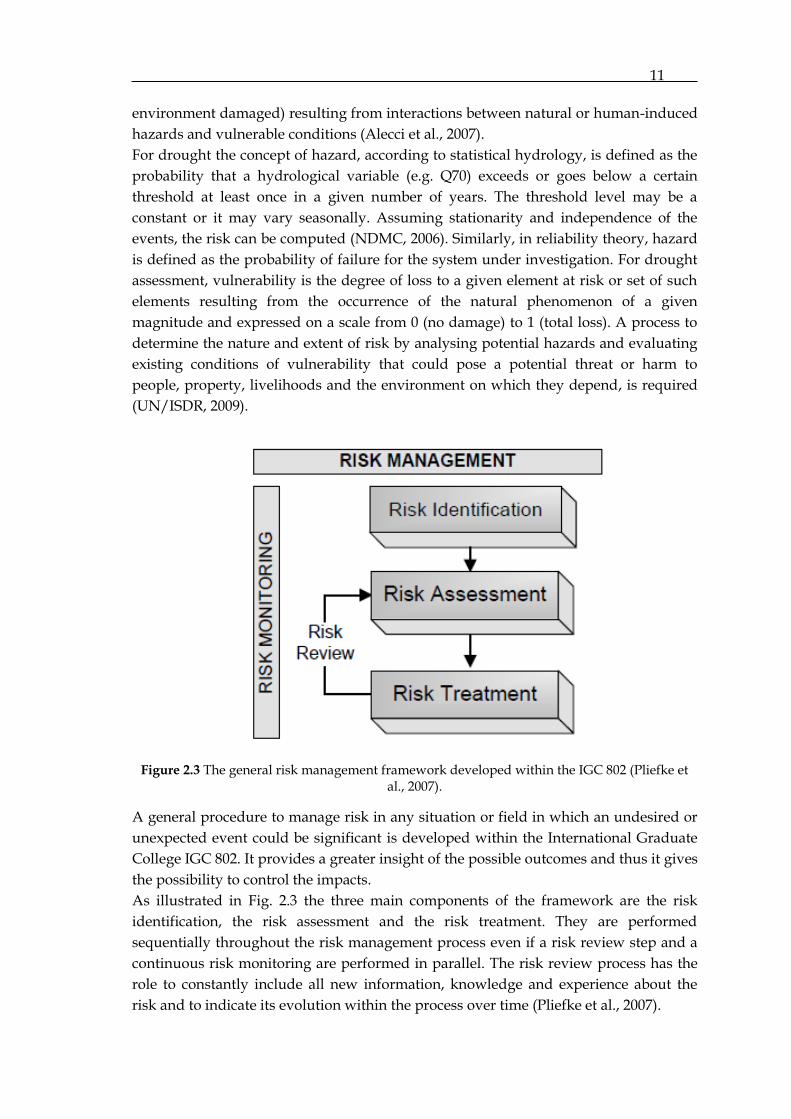


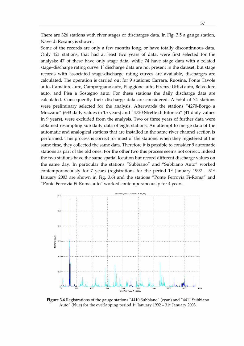


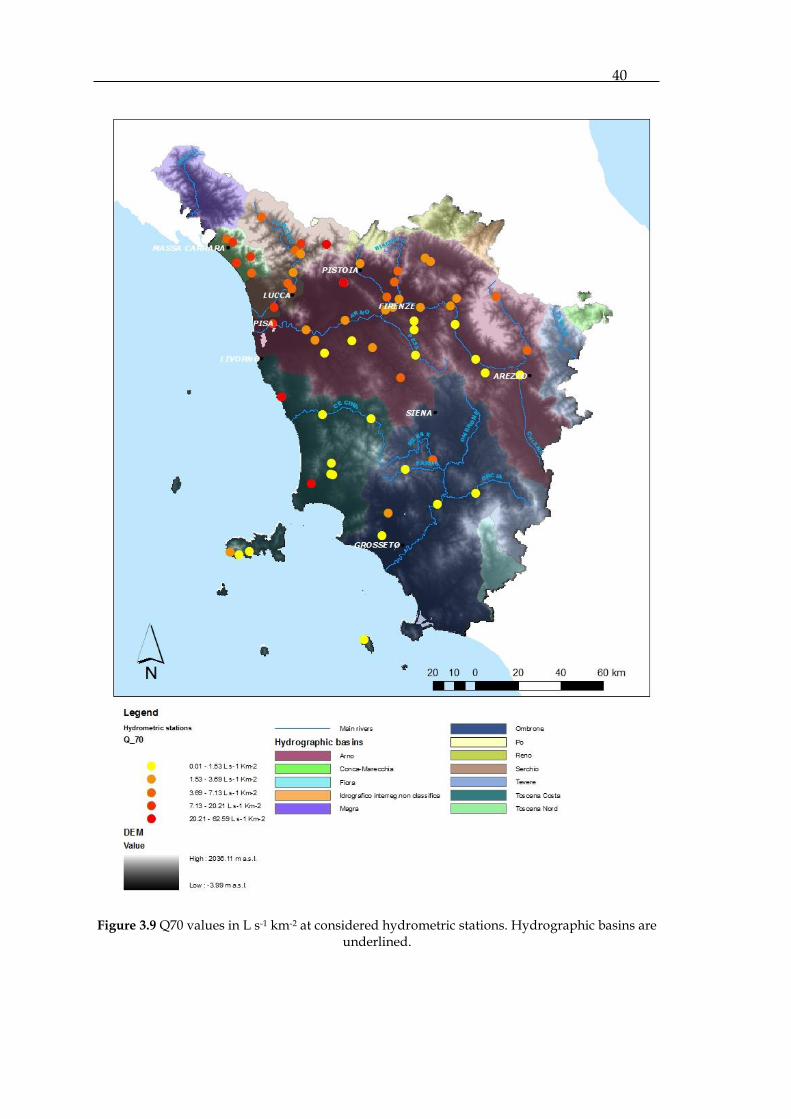


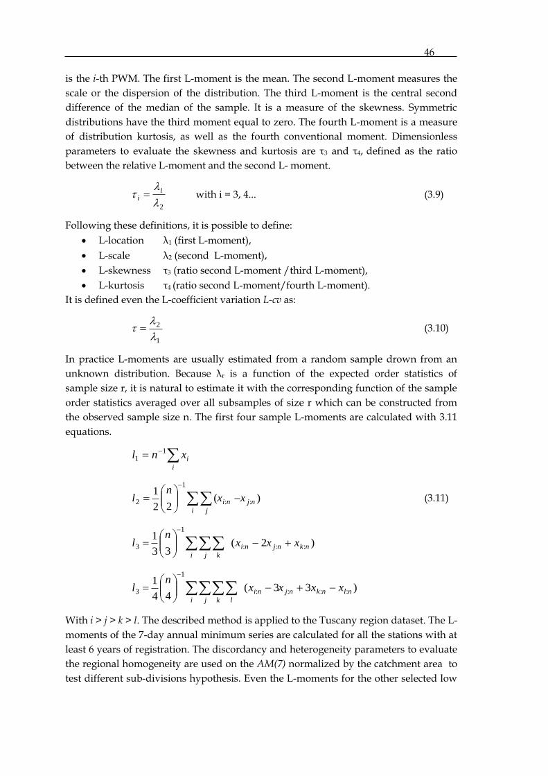


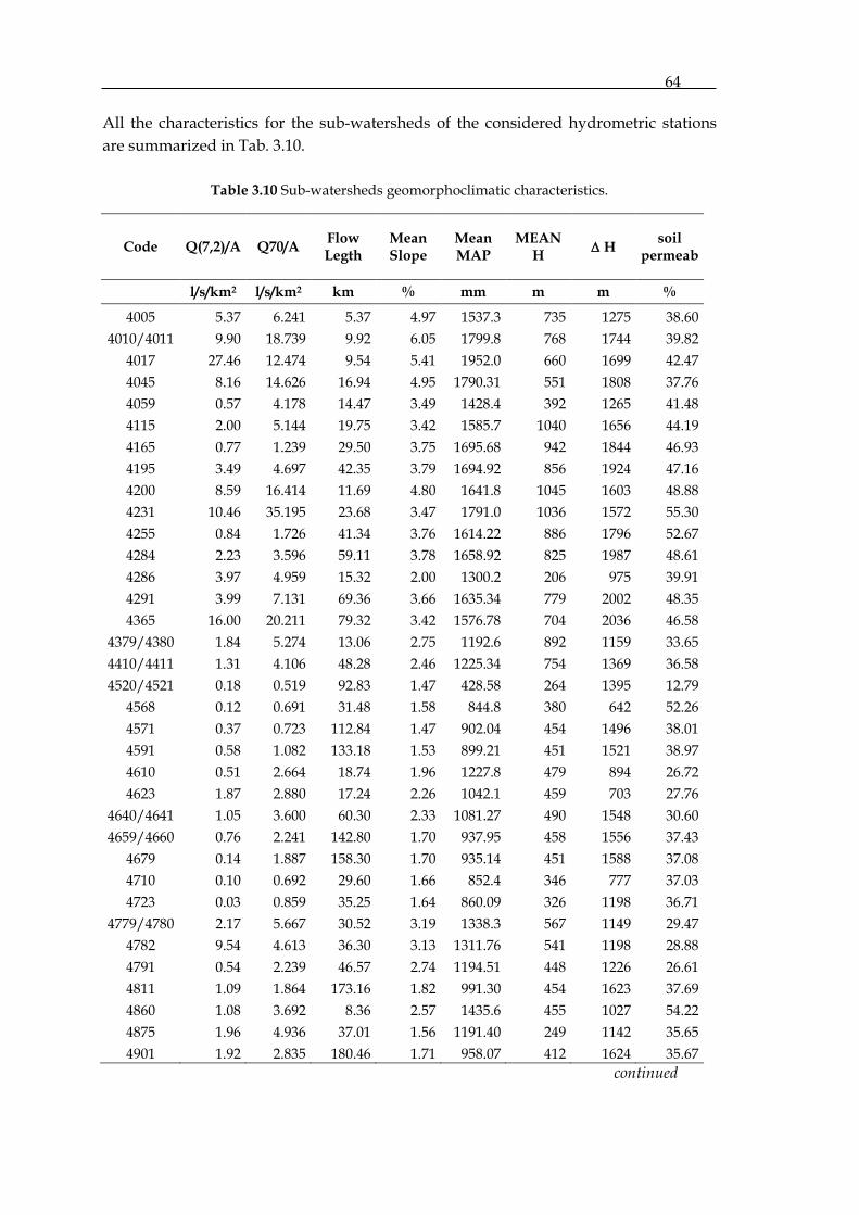

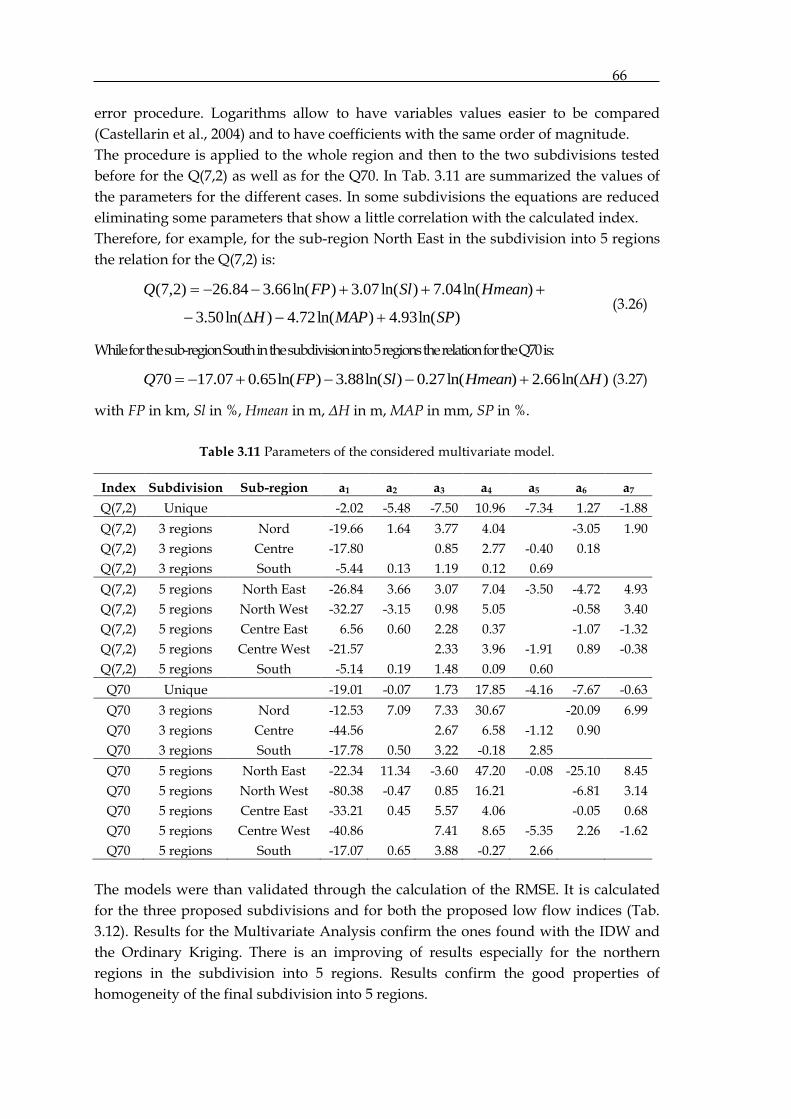


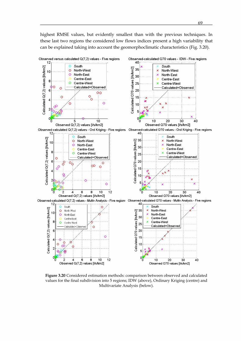


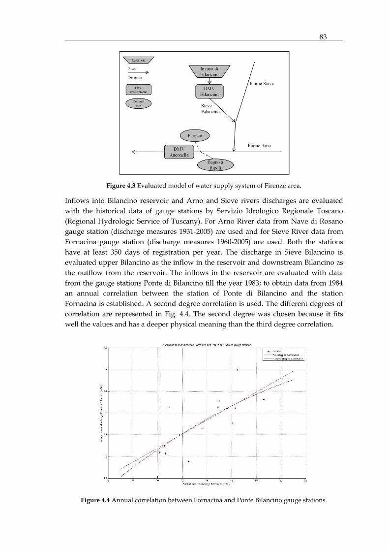


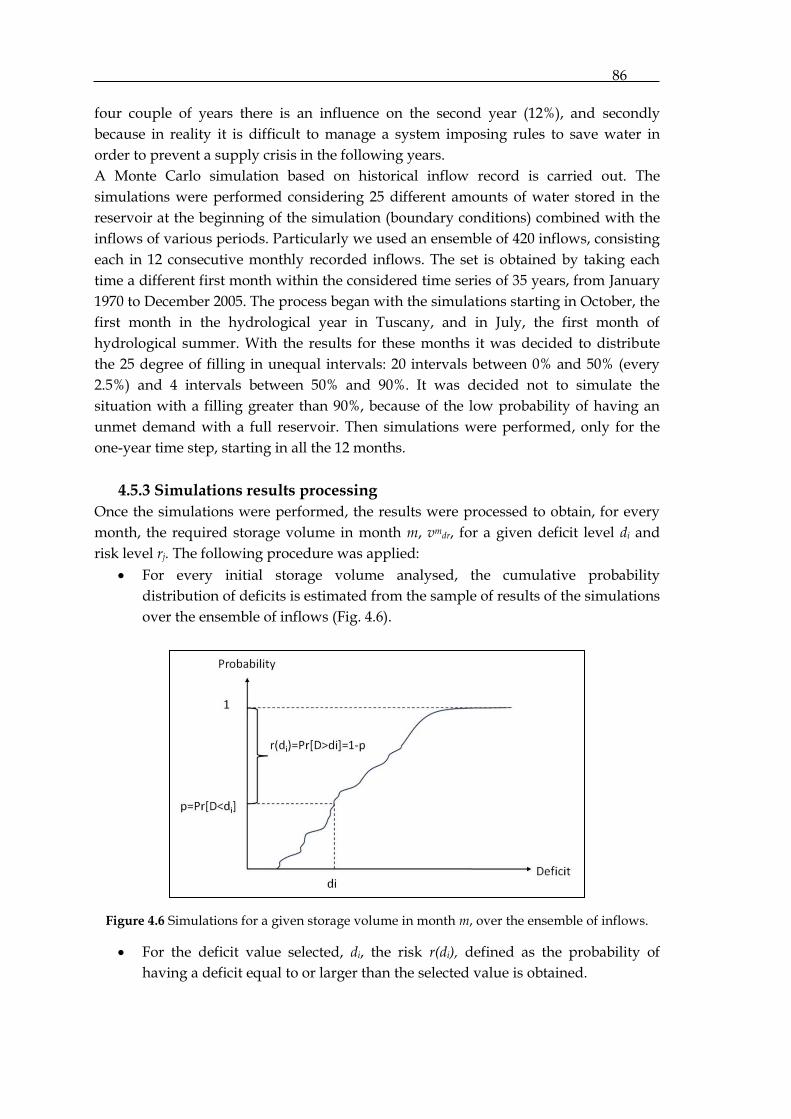


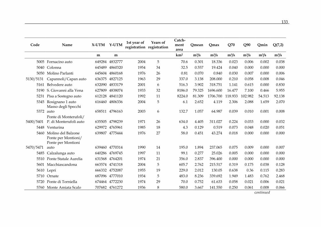


![mitmachen[youknowit]helikon-online.de Hannes Liebrandt (2014): Napoleon I. und sein kontroverses Verhältnis zur Religion. Versuch einer historischen Einordnung. Geschichte, Gesellschaft](https://static.documents.pub/doc/80x56/60cc88940d18d66bca7fcc44/mitmachenyouknowithelikon-onlinede-hannes-liebrandt-2014-napoleon-i-und-sein.jpg)

