Page 1
Dual methods for functionswith bounded variation
Yurii Nesterov, CORE/INMA (UCL)
April 3, 2013, GaTech, Atlanta
Joint work with A.Gasnikov (MIPT, Moscow)
Yu. Nesterov Functions with bounded variation 1/19
Page 2
Outline
1 Problem formulation
2 Bounds on the dual solution
3 Problems with bounded variation
4 Modified Gradient Methods
5 Fast Gradient Method
6 Examples
Yu. Nesterov Functions with bounded variation 2/19
Page 3
Problem formulation
Problem:
(P) : f∗def= min
x∈Q{f(x) : Ax = b},
Q ⊂ X is a simple closed convex set,function f(·) is strongly convex on Q:
f(y) ≥ f(x) + 〈∇f(x), y − x〉+ 12σ(f)‖y − x‖2, x, y ∈ Q.
A : X → Y ∗ is a linear operator, and b ∈ Y ∗.
Approximate solution: find x ∈ Q such that
f(x)− f∗ ≤ εf , ‖Ax− b‖ ≤ εg.
Yu. Nesterov Functions with bounded variation 3/19
Page 4
Problem formulation
Problem:
(P) : f∗def= min
x∈Q{f(x) : Ax = b},
Q ⊂ X is a simple closed convex set,
function f(·) is strongly convex on Q:
f(y) ≥ f(x) + 〈∇f(x), y − x〉+ 12σ(f)‖y − x‖2, x, y ∈ Q.
A : X → Y ∗ is a linear operator, and b ∈ Y ∗.
Approximate solution: find x ∈ Q such that
f(x)− f∗ ≤ εf , ‖Ax− b‖ ≤ εg.
Yu. Nesterov Functions with bounded variation 3/19
Page 5
Problem formulation
Problem:
(P) : f∗def= min
x∈Q{f(x) : Ax = b},
Q ⊂ X is a simple closed convex set,function f(·) is strongly convex on Q:
f(y) ≥ f(x) + 〈∇f(x), y − x〉+ 12σ(f)‖y − x‖2, x, y ∈ Q.
A : X → Y ∗ is a linear operator, and b ∈ Y ∗.
Approximate solution: find x ∈ Q such that
f(x)− f∗ ≤ εf , ‖Ax− b‖ ≤ εg.
Yu. Nesterov Functions with bounded variation 3/19
Page 6
Problem formulation
Problem:
(P) : f∗def= min
x∈Q{f(x) : Ax = b},
Q ⊂ X is a simple closed convex set,function f(·) is strongly convex on Q:
f(y) ≥ f(x) + 〈∇f(x), y − x〉+ 12σ(f)‖y − x‖2, x, y ∈ Q.
A : X → Y ∗ is a linear operator, and b ∈ Y ∗.
Approximate solution: find x ∈ Q such that
f(x)− f∗ ≤ εf , ‖Ax− b‖ ≤ εg.
Yu. Nesterov Functions with bounded variation 3/19
Page 7
Problem formulation
Problem:
(P) : f∗def= min
x∈Q{f(x) : Ax = b},
Q ⊂ X is a simple closed convex set,function f(·) is strongly convex on Q:
f(y) ≥ f(x) + 〈∇f(x), y − x〉+ 12σ(f)‖y − x‖2, x, y ∈ Q.
A : X → Y ∗ is a linear operator, and b ∈ Y ∗.
Approximate solution: find x ∈ Q such that
f(x)− f∗ ≤ εf , ‖Ax− b‖ ≤ εg.
Yu. Nesterov Functions with bounded variation 3/19
Page 8
Complexity of problem (P): Black Box model
Assume for a moment that all norms are Euclidean.If A ≡ ∅, ‖∇f(x)‖∗ ≤ L, and x ∈ Q, then we need
O(
L2
εf σ(f)
)iterations.
If f ≡ const, then we need O(
1εg‖A‖ diamQ
)iterations.
(Minimize the squared residual by FGM).
Define nonsmooth functional constraintg(x) = ‖Ax− b‖ ≤ 0.
Standard subgradient method ensures
O
([Lεf
+ ‖A‖εg
]2diam2Q
)iterations.
Yu. Nesterov Functions with bounded variation 4/19
Page 9
Complexity of problem (P): Black Box model
Assume for a moment that all norms are Euclidean.
If A ≡ ∅, ‖∇f(x)‖∗ ≤ L, and x ∈ Q, then we needO(
L2
εf σ(f)
)iterations.
If f ≡ const, then we need O(
1εg‖A‖ diamQ
)iterations.
(Minimize the squared residual by FGM).
Define nonsmooth functional constraintg(x) = ‖Ax− b‖ ≤ 0.
Standard subgradient method ensures
O
([Lεf
+ ‖A‖εg
]2diam2Q
)iterations.
Yu. Nesterov Functions with bounded variation 4/19
Page 10
Complexity of problem (P): Black Box model
Assume for a moment that all norms are Euclidean.If A ≡ ∅, ‖∇f(x)‖∗ ≤ L, and x ∈ Q, then we need
O(
L2
εf σ(f)
)iterations.
If f ≡ const, then we need O(
1εg‖A‖ diamQ
)iterations.
(Minimize the squared residual by FGM).
Define nonsmooth functional constraintg(x) = ‖Ax− b‖ ≤ 0.
Standard subgradient method ensures
O
([Lεf
+ ‖A‖εg
]2diam2Q
)iterations.
Yu. Nesterov Functions with bounded variation 4/19
Page 11
Complexity of problem (P): Black Box model
Assume for a moment that all norms are Euclidean.If A ≡ ∅, ‖∇f(x)‖∗ ≤ L, and x ∈ Q, then we need
O(
L2
εf σ(f)
)iterations.
If f ≡ const, then we need O(
1εg‖A‖ diamQ
)iterations.
(Minimize the squared residual by FGM).
Define nonsmooth functional constraintg(x) = ‖Ax− b‖ ≤ 0.
Standard subgradient method ensures
O
([Lεf
+ ‖A‖εg
]2diam2Q
)iterations.
Yu. Nesterov Functions with bounded variation 4/19
Page 12
Complexity of problem (P): Black Box model
Assume for a moment that all norms are Euclidean.If A ≡ ∅, ‖∇f(x)‖∗ ≤ L, and x ∈ Q, then we need
O(
L2
εf σ(f)
)iterations.
If f ≡ const, then we need O(
1εg‖A‖ diamQ
)iterations.
(Minimize the squared residual by FGM).
Define nonsmooth functional constraintg(x) = ‖Ax− b‖ ≤ 0.
Standard subgradient method ensures
O
([Lεf
+ ‖A‖εg
]2diam2Q
)iterations.
Yu. Nesterov Functions with bounded variation 4/19
Page 13
Complexity of problem (P): Black Box model
Assume for a moment that all norms are Euclidean.If A ≡ ∅, ‖∇f(x)‖∗ ≤ L, and x ∈ Q, then we need
O(
L2
εf σ(f)
)iterations.
If f ≡ const, then we need O(
1εg‖A‖ diamQ
)iterations.
(Minimize the squared residual by FGM).
Define nonsmooth functional constraintg(x) = ‖Ax− b‖ ≤ 0.
Standard subgradient method ensures
O
([Lεf
+ ‖A‖εg
]2diam2Q
)iterations.
Yu. Nesterov Functions with bounded variation 4/19
Page 14
Complexity of problem (P): Black Box model
Assume for a moment that all norms are Euclidean.If A ≡ ∅, ‖∇f(x)‖∗ ≤ L, and x ∈ Q, then we need
O(
L2
εf σ(f)
)iterations.
If f ≡ const, then we need O(
1εg‖A‖ diamQ
)iterations.
(Minimize the squared residual by FGM).
Define nonsmooth functional constraintg(x) = ‖Ax− b‖ ≤ 0.
Standard subgradient method ensures
O
([Lεf
+ ‖A‖εg
]2diam2Q
)iterations.
Yu. Nesterov Functions with bounded variation 4/19
Page 15
Dual approach
Define the Lagrangian L(x, y) = f(x) + 〈b−Ax, y〉. The dualproblem is as follows:
φ(y) def= minx∈QL(x, y), φ∗
def= supy∈Y
φ(y).
NB: This is useful only if φ(y) can be easily computed.
Since f is strongly convex, φ(y) is well defined for any y ∈ Y :φ(y) = L(x(y), y), ∇φ(y) = b−Ax(y), y ∈ Y ,
where the point x(y) ∈ Q is uniquely defined. Its gradient isLipschitz continuous with L(φ) = 1
σ(f)‖A‖2.
But: the standard complexity bounds of GMs depend on y∗:Choosing y0 = 0, we have φ(y∗)− φ(yk) ≤ 4L(φ)‖y∗‖2
(k+1)2.
NB: ‖y∗‖ can be big!
Yu. Nesterov Functions with bounded variation 5/19
Page 16
Dual approach
Define the Lagrangian L(x, y) = f(x) + 〈b−Ax, y〉.
The dualproblem is as follows:
φ(y) def= minx∈QL(x, y), φ∗
def= supy∈Y
φ(y).
NB: This is useful only if φ(y) can be easily computed.
Since f is strongly convex, φ(y) is well defined for any y ∈ Y :φ(y) = L(x(y), y), ∇φ(y) = b−Ax(y), y ∈ Y ,
where the point x(y) ∈ Q is uniquely defined. Its gradient isLipschitz continuous with L(φ) = 1
σ(f)‖A‖2.
But: the standard complexity bounds of GMs depend on y∗:Choosing y0 = 0, we have φ(y∗)− φ(yk) ≤ 4L(φ)‖y∗‖2
(k+1)2.
NB: ‖y∗‖ can be big!
Yu. Nesterov Functions with bounded variation 5/19
Page 17
Dual approach
Define the Lagrangian L(x, y) = f(x) + 〈b−Ax, y〉. The dualproblem is as follows:
φ(y) def= minx∈QL(x, y), φ∗
def= supy∈Y
φ(y).
NB: This is useful only if φ(y) can be easily computed.
Since f is strongly convex, φ(y) is well defined for any y ∈ Y :φ(y) = L(x(y), y), ∇φ(y) = b−Ax(y), y ∈ Y ,
where the point x(y) ∈ Q is uniquely defined. Its gradient isLipschitz continuous with L(φ) = 1
σ(f)‖A‖2.
But: the standard complexity bounds of GMs depend on y∗:Choosing y0 = 0, we have φ(y∗)− φ(yk) ≤ 4L(φ)‖y∗‖2
(k+1)2.
NB: ‖y∗‖ can be big!
Yu. Nesterov Functions with bounded variation 5/19
Page 18
Dual approach
Define the Lagrangian L(x, y) = f(x) + 〈b−Ax, y〉. The dualproblem is as follows:
φ(y) def= minx∈QL(x, y), φ∗
def= supy∈Y
φ(y).
NB: This is useful only if φ(y) can be easily computed.
Since f is strongly convex, φ(y) is well defined for any y ∈ Y :φ(y) = L(x(y), y), ∇φ(y) = b−Ax(y), y ∈ Y ,
where the point x(y) ∈ Q is uniquely defined. Its gradient isLipschitz continuous with L(φ) = 1
σ(f)‖A‖2.
But: the standard complexity bounds of GMs depend on y∗:Choosing y0 = 0, we have φ(y∗)− φ(yk) ≤ 4L(φ)‖y∗‖2
(k+1)2.
NB: ‖y∗‖ can be big!
Yu. Nesterov Functions with bounded variation 5/19
Page 19
Dual approach
Define the Lagrangian L(x, y) = f(x) + 〈b−Ax, y〉. The dualproblem is as follows:
φ(y) def= minx∈QL(x, y), φ∗
def= supy∈Y
φ(y).
NB: This is useful only if φ(y) can be easily computed.
Since f is strongly convex, φ(y) is well defined for any y ∈ Y :
φ(y) = L(x(y), y), ∇φ(y) = b−Ax(y), y ∈ Y ,where the point x(y) ∈ Q is uniquely defined. Its gradient isLipschitz continuous with L(φ) = 1
σ(f)‖A‖2.
But: the standard complexity bounds of GMs depend on y∗:Choosing y0 = 0, we have φ(y∗)− φ(yk) ≤ 4L(φ)‖y∗‖2
(k+1)2.
NB: ‖y∗‖ can be big!
Yu. Nesterov Functions with bounded variation 5/19
Page 20
Dual approach
Define the Lagrangian L(x, y) = f(x) + 〈b−Ax, y〉. The dualproblem is as follows:
φ(y) def= minx∈QL(x, y), φ∗
def= supy∈Y
φ(y).
NB: This is useful only if φ(y) can be easily computed.
Since f is strongly convex, φ(y) is well defined for any y ∈ Y :φ(y) = L(x(y), y), ∇φ(y) = b−Ax(y), y ∈ Y ,
where the point x(y) ∈ Q is uniquely defined.
Its gradient isLipschitz continuous with L(φ) = 1
σ(f)‖A‖2.
But: the standard complexity bounds of GMs depend on y∗:Choosing y0 = 0, we have φ(y∗)− φ(yk) ≤ 4L(φ)‖y∗‖2
(k+1)2.
NB: ‖y∗‖ can be big!
Yu. Nesterov Functions with bounded variation 5/19
Page 21
Dual approach
Define the Lagrangian L(x, y) = f(x) + 〈b−Ax, y〉. The dualproblem is as follows:
φ(y) def= minx∈QL(x, y), φ∗
def= supy∈Y
φ(y).
NB: This is useful only if φ(y) can be easily computed.
Since f is strongly convex, φ(y) is well defined for any y ∈ Y :φ(y) = L(x(y), y), ∇φ(y) = b−Ax(y), y ∈ Y ,
where the point x(y) ∈ Q is uniquely defined. Its gradient isLipschitz continuous with L(φ) = 1
σ(f)‖A‖2.
But: the standard complexity bounds of GMs depend on y∗:Choosing y0 = 0, we have φ(y∗)− φ(yk) ≤ 4L(φ)‖y∗‖2
(k+1)2.
NB: ‖y∗‖ can be big!
Yu. Nesterov Functions with bounded variation 5/19
Page 22
Dual approach
Define the Lagrangian L(x, y) = f(x) + 〈b−Ax, y〉. The dualproblem is as follows:
φ(y) def= minx∈QL(x, y), φ∗
def= supy∈Y
φ(y).
NB: This is useful only if φ(y) can be easily computed.
Since f is strongly convex, φ(y) is well defined for any y ∈ Y :φ(y) = L(x(y), y), ∇φ(y) = b−Ax(y), y ∈ Y ,
where the point x(y) ∈ Q is uniquely defined. Its gradient isLipschitz continuous with L(φ) = 1
σ(f)‖A‖2.
But:
the standard complexity bounds of GMs depend on y∗:Choosing y0 = 0, we have φ(y∗)− φ(yk) ≤ 4L(φ)‖y∗‖2
(k+1)2.
NB: ‖y∗‖ can be big!
Yu. Nesterov Functions with bounded variation 5/19
Page 23
Dual approach
Define the Lagrangian L(x, y) = f(x) + 〈b−Ax, y〉. The dualproblem is as follows:
φ(y) def= minx∈QL(x, y), φ∗
def= supy∈Y
φ(y).
NB: This is useful only if φ(y) can be easily computed.
Since f is strongly convex, φ(y) is well defined for any y ∈ Y :φ(y) = L(x(y), y), ∇φ(y) = b−Ax(y), y ∈ Y ,
where the point x(y) ∈ Q is uniquely defined. Its gradient isLipschitz continuous with L(φ) = 1
σ(f)‖A‖2.
But: the standard complexity bounds of GMs depend on y∗:
Choosing y0 = 0, we have φ(y∗)− φ(yk) ≤ 4L(φ)‖y∗‖2(k+1)2
.
NB: ‖y∗‖ can be big!
Yu. Nesterov Functions with bounded variation 5/19
Page 24
Dual approach
Define the Lagrangian L(x, y) = f(x) + 〈b−Ax, y〉. The dualproblem is as follows:
φ(y) def= minx∈QL(x, y), φ∗
def= supy∈Y
φ(y).
NB: This is useful only if φ(y) can be easily computed.
Since f is strongly convex, φ(y) is well defined for any y ∈ Y :φ(y) = L(x(y), y), ∇φ(y) = b−Ax(y), y ∈ Y ,
where the point x(y) ∈ Q is uniquely defined. Its gradient isLipschitz continuous with L(φ) = 1
σ(f)‖A‖2.
But: the standard complexity bounds of GMs depend on y∗:Choosing y0 = 0,
we have φ(y∗)− φ(yk) ≤ 4L(φ)‖y∗‖2(k+1)2
.
NB: ‖y∗‖ can be big!
Yu. Nesterov Functions with bounded variation 5/19
Page 25
Dual approach
Define the Lagrangian L(x, y) = f(x) + 〈b−Ax, y〉. The dualproblem is as follows:
φ(y) def= minx∈QL(x, y), φ∗
def= supy∈Y
φ(y).
NB: This is useful only if φ(y) can be easily computed.
Since f is strongly convex, φ(y) is well defined for any y ∈ Y :φ(y) = L(x(y), y), ∇φ(y) = b−Ax(y), y ∈ Y ,
where the point x(y) ∈ Q is uniquely defined. Its gradient isLipschitz continuous with L(φ) = 1
σ(f)‖A‖2.
But: the standard complexity bounds of GMs depend on y∗:Choosing y0 = 0, we have φ(y∗)− φ(yk) ≤ 4L(φ)‖y∗‖2
(k+1)2.
NB: ‖y∗‖ can be big!
Yu. Nesterov Functions with bounded variation 5/19
Page 26
Dual approach
Define the Lagrangian L(x, y) = f(x) + 〈b−Ax, y〉. The dualproblem is as follows:
φ(y) def= minx∈QL(x, y), φ∗
def= supy∈Y
φ(y).
NB: This is useful only if φ(y) can be easily computed.
Since f is strongly convex, φ(y) is well defined for any y ∈ Y :φ(y) = L(x(y), y), ∇φ(y) = b−Ax(y), y ∈ Y ,
where the point x(y) ∈ Q is uniquely defined. Its gradient isLipschitz continuous with L(φ) = 1
σ(f)‖A‖2.
But: the standard complexity bounds of GMs depend on y∗:Choosing y0 = 0, we have φ(y∗)− φ(yk) ≤ 4L(φ)‖y∗‖2
(k+1)2.
NB: ‖y∗‖ can be big!
Yu. Nesterov Functions with bounded variation 5/19
Page 27
Example
Let E = R2, and ‖x‖ ≡ ‖x‖2. Consider the problem
minx
{f(x) = 1
2‖x− e2‖2 : x(1) = 1, ‖x‖ ≤ 1}
.
Defining the LagrangianL(x, y) = 1
2‖x− e2‖2 + y(1−x(1)) = 12‖x− e2− ye1‖2 + y− 1
2y2,
we get x(y) = x(y)/‖x(y)‖, where x(y) = e2 + ye1.
Thus, φ(y) = 12(‖x(y)‖ − 1)2 + y − 1
2y2 = 1− 1
y+√
1+y2.
No duality gap and φ(y)→ f∗ = 1 as y →∞.x(y)→ x∗ = e1 as y →∞.Optimal solution does not exist. Rate of convergence ofthe standard dual GMs = ?
Yu. Nesterov Functions with bounded variation 6/19
Page 28
Example
Let E = R2, and ‖x‖ ≡ ‖x‖2.
Consider the problem
minx
{f(x) = 1
2‖x− e2‖2 : x(1) = 1, ‖x‖ ≤ 1}
.
Defining the LagrangianL(x, y) = 1
2‖x− e2‖2 + y(1−x(1)) = 12‖x− e2− ye1‖2 + y− 1
2y2,
we get x(y) = x(y)/‖x(y)‖, where x(y) = e2 + ye1.
Thus, φ(y) = 12(‖x(y)‖ − 1)2 + y − 1
2y2 = 1− 1
y+√
1+y2.
No duality gap and φ(y)→ f∗ = 1 as y →∞.x(y)→ x∗ = e1 as y →∞.Optimal solution does not exist. Rate of convergence ofthe standard dual GMs = ?
Yu. Nesterov Functions with bounded variation 6/19
Page 29
Example
Let E = R2, and ‖x‖ ≡ ‖x‖2. Consider the problem
minx
{f(x) = 1
2‖x− e2‖2 : x(1) = 1, ‖x‖ ≤ 1}
.
Defining the LagrangianL(x, y) = 1
2‖x− e2‖2 + y(1−x(1)) = 12‖x− e2− ye1‖2 + y− 1
2y2,
we get x(y) = x(y)/‖x(y)‖, where x(y) = e2 + ye1.
Thus, φ(y) = 12(‖x(y)‖ − 1)2 + y − 1
2y2 = 1− 1
y+√
1+y2.
No duality gap and φ(y)→ f∗ = 1 as y →∞.x(y)→ x∗ = e1 as y →∞.Optimal solution does not exist. Rate of convergence ofthe standard dual GMs = ?
Yu. Nesterov Functions with bounded variation 6/19
Page 30
Example
Let E = R2, and ‖x‖ ≡ ‖x‖2. Consider the problem
minx
{f(x) = 1
2‖x− e2‖2 : x(1) = 1, ‖x‖ ≤ 1}
.
Defining the LagrangianL(x, y) = 1
2‖x− e2‖2 + y(1−x(1)) = 12‖x− e2− ye1‖2 + y− 1
2y2,
we get x(y) = x(y)/‖x(y)‖, where x(y) = e2 + ye1.
Thus, φ(y) = 12(‖x(y)‖ − 1)2 + y − 1
2y2 = 1− 1
y+√
1+y2.
No duality gap and φ(y)→ f∗ = 1 as y →∞.x(y)→ x∗ = e1 as y →∞.Optimal solution does not exist. Rate of convergence ofthe standard dual GMs = ?
Yu. Nesterov Functions with bounded variation 6/19
Page 31
Example
Let E = R2, and ‖x‖ ≡ ‖x‖2. Consider the problem
minx
{f(x) = 1
2‖x− e2‖2 : x(1) = 1, ‖x‖ ≤ 1}
.
Defining the LagrangianL(x, y) = 1
2‖x− e2‖2 + y(1−x(1)) = 12‖x− e2− ye1‖2 + y− 1
2y2,
we get x(y) = x(y)/‖x(y)‖, where x(y) = e2 + ye1.
Thus, φ(y) = 12(‖x(y)‖ − 1)2 + y − 1
2y2 = 1− 1
y+√
1+y2.
No duality gap and φ(y)→ f∗ = 1 as y →∞.x(y)→ x∗ = e1 as y →∞.Optimal solution does not exist. Rate of convergence ofthe standard dual GMs = ?
Yu. Nesterov Functions with bounded variation 6/19
Page 32
Example
Let E = R2, and ‖x‖ ≡ ‖x‖2. Consider the problem
minx
{f(x) = 1
2‖x− e2‖2 : x(1) = 1, ‖x‖ ≤ 1}
.
Defining the LagrangianL(x, y) = 1
2‖x− e2‖2 + y(1−x(1)) = 12‖x− e2− ye1‖2 + y− 1
2y2,
we get x(y) = x(y)/‖x(y)‖, where x(y) = e2 + ye1.
Thus, φ(y) = 12(‖x(y)‖ − 1)2 + y − 1
2y2 = 1− 1
y+√
1+y2.
No duality gap and φ(y)→ f∗ = 1 as y →∞.
x(y)→ x∗ = e1 as y →∞.Optimal solution does not exist. Rate of convergence ofthe standard dual GMs = ?
Yu. Nesterov Functions with bounded variation 6/19
Page 33
Example
Let E = R2, and ‖x‖ ≡ ‖x‖2. Consider the problem
minx
{f(x) = 1
2‖x− e2‖2 : x(1) = 1, ‖x‖ ≤ 1}
.
Defining the LagrangianL(x, y) = 1
2‖x− e2‖2 + y(1−x(1)) = 12‖x− e2− ye1‖2 + y− 1
2y2,
we get x(y) = x(y)/‖x(y)‖, where x(y) = e2 + ye1.
Thus, φ(y) = 12(‖x(y)‖ − 1)2 + y − 1
2y2 = 1− 1
y+√
1+y2.
No duality gap and φ(y)→ f∗ = 1 as y →∞.x(y)→ x∗ = e1 as y →∞.
Optimal solution does not exist. Rate of convergence ofthe standard dual GMs = ?
Yu. Nesterov Functions with bounded variation 6/19
Page 34
Example
Let E = R2, and ‖x‖ ≡ ‖x‖2. Consider the problem
minx
{f(x) = 1
2‖x− e2‖2 : x(1) = 1, ‖x‖ ≤ 1}
.
Defining the LagrangianL(x, y) = 1
2‖x− e2‖2 + y(1−x(1)) = 12‖x− e2− ye1‖2 + y− 1
2y2,
we get x(y) = x(y)/‖x(y)‖, where x(y) = e2 + ye1.
Thus, φ(y) = 12(‖x(y)‖ − 1)2 + y − 1
2y2 = 1− 1
y+√
1+y2.
No duality gap and φ(y)→ f∗ = 1 as y →∞.x(y)→ x∗ = e1 as y →∞.Optimal solution does not exist.
Rate of convergence ofthe standard dual GMs = ?
Yu. Nesterov Functions with bounded variation 6/19
Page 35
Example
Let E = R2, and ‖x‖ ≡ ‖x‖2. Consider the problem
minx
{f(x) = 1
2‖x− e2‖2 : x(1) = 1, ‖x‖ ≤ 1}
.
Defining the LagrangianL(x, y) = 1
2‖x− e2‖2 + y(1−x(1)) = 12‖x− e2− ye1‖2 + y− 1
2y2,
we get x(y) = x(y)/‖x(y)‖, where x(y) = e2 + ye1.
Thus, φ(y) = 12(‖x(y)‖ − 1)2 + y − 1
2y2 = 1− 1
y+√
1+y2.
No duality gap and φ(y)→ f∗ = 1 as y →∞.x(y)→ x∗ = e1 as y →∞.Optimal solution does not exist. Rate of convergence ofthe standard dual GMs = ?
Yu. Nesterov Functions with bounded variation 6/19
Page 36
Bounding the dual solution
Assumption 1: ∃x and a radius ρ > 0 such that
Ax = b and B(x, ρ) ⊆ Q.
Lemma. ‖AT y∗‖ ≤ (1 + 1ρD)‖∇f(x∗)‖∗ , where D = diamQ.
Proof: since 〈∇f(x∗)−AT y∗, x− x∗〉 ≥ 0, for all x ∈ Q wehave
0 ≤ 〈∇f(x∗)−AT y∗, x− x∗〉+ 〈∇f(x∗)−AT y∗, x− x〉= 〈∇f(x∗), x− x∗〉+ 〈∇f(x∗)−AT y∗, x− x〉.
Restricting ourselves to x ∈ B(x, ρ), we obtain
ρ‖∇f(x∗)−AT y∗‖∗ ≤ 〈∇f(x∗), x− x∗〉 ≤ ‖∇f(x∗)‖∗ ·D.
Hence, ‖∇f(x∗)‖∗ ·D ≥ ρ‖AT y∗‖∗ − ρ‖∇f(x∗)‖∗.NB: We need ‖∇f(x)‖∗ ≤ const. (This may not happen.)
Yu. Nesterov Functions with bounded variation 7/19
Page 37
Bounding the dual solution
Assumption 1: ∃x and a radius ρ > 0 such that
Ax = b and B(x, ρ) ⊆ Q.
Lemma. ‖AT y∗‖ ≤ (1 + 1ρD)‖∇f(x∗)‖∗ , where D = diamQ.
Proof: since 〈∇f(x∗)−AT y∗, x− x∗〉 ≥ 0, for all x ∈ Q wehave
0 ≤ 〈∇f(x∗)−AT y∗, x− x∗〉+ 〈∇f(x∗)−AT y∗, x− x〉= 〈∇f(x∗), x− x∗〉+ 〈∇f(x∗)−AT y∗, x− x〉.
Restricting ourselves to x ∈ B(x, ρ), we obtain
ρ‖∇f(x∗)−AT y∗‖∗ ≤ 〈∇f(x∗), x− x∗〉 ≤ ‖∇f(x∗)‖∗ ·D.
Hence, ‖∇f(x∗)‖∗ ·D ≥ ρ‖AT y∗‖∗ − ρ‖∇f(x∗)‖∗.NB: We need ‖∇f(x)‖∗ ≤ const. (This may not happen.)
Yu. Nesterov Functions with bounded variation 7/19
Page 38
Bounding the dual solution
Assumption 1: ∃x and a radius ρ > 0 such that
Ax = b and B(x, ρ) ⊆ Q.
Lemma. ‖AT y∗‖ ≤ (1 + 1ρD)‖∇f(x∗)‖∗ , where D = diamQ.
Proof: since 〈∇f(x∗)−AT y∗, x− x∗〉 ≥ 0, for all x ∈ Q wehave
0 ≤ 〈∇f(x∗)−AT y∗, x− x∗〉+ 〈∇f(x∗)−AT y∗, x− x〉= 〈∇f(x∗), x− x∗〉+ 〈∇f(x∗)−AT y∗, x− x〉.
Restricting ourselves to x ∈ B(x, ρ), we obtain
ρ‖∇f(x∗)−AT y∗‖∗ ≤ 〈∇f(x∗), x− x∗〉 ≤ ‖∇f(x∗)‖∗ ·D.
Hence, ‖∇f(x∗)‖∗ ·D ≥ ρ‖AT y∗‖∗ − ρ‖∇f(x∗)‖∗.NB: We need ‖∇f(x)‖∗ ≤ const. (This may not happen.)
Yu. Nesterov Functions with bounded variation 7/19
Page 39
Bounding the dual solution
Assumption 1: ∃x and a radius ρ > 0 such that
Ax = b and B(x, ρ) ⊆ Q.
Lemma. ‖AT y∗‖ ≤ (1 + 1ρD)‖∇f(x∗)‖∗ , where D = diamQ.
Proof: since 〈∇f(x∗)−AT y∗, x− x∗〉 ≥ 0, for all x ∈ Q wehave
0 ≤ 〈∇f(x∗)−AT y∗, x− x∗〉+ 〈∇f(x∗)−AT y∗, x− x〉= 〈∇f(x∗), x− x∗〉+ 〈∇f(x∗)−AT y∗, x− x〉.
Restricting ourselves to x ∈ B(x, ρ), we obtain
ρ‖∇f(x∗)−AT y∗‖∗ ≤ 〈∇f(x∗), x− x∗〉 ≤ ‖∇f(x∗)‖∗ ·D.
Hence, ‖∇f(x∗)‖∗ ·D ≥ ρ‖AT y∗‖∗ − ρ‖∇f(x∗)‖∗.NB: We need ‖∇f(x)‖∗ ≤ const. (This may not happen.)
Yu. Nesterov Functions with bounded variation 7/19
Page 40
Bounding the dual solution
Assumption 1: ∃x and a radius ρ > 0 such that
Ax = b and B(x, ρ) ⊆ Q.
Lemma. ‖AT y∗‖ ≤ (1 + 1ρD)‖∇f(x∗)‖∗ , where D = diamQ.
Proof: since 〈∇f(x∗)−AT y∗, x− x∗〉 ≥ 0,
for all x ∈ Q wehave
0 ≤ 〈∇f(x∗)−AT y∗, x− x∗〉+ 〈∇f(x∗)−AT y∗, x− x〉= 〈∇f(x∗), x− x∗〉+ 〈∇f(x∗)−AT y∗, x− x〉.
Restricting ourselves to x ∈ B(x, ρ), we obtain
ρ‖∇f(x∗)−AT y∗‖∗ ≤ 〈∇f(x∗), x− x∗〉 ≤ ‖∇f(x∗)‖∗ ·D.
Hence, ‖∇f(x∗)‖∗ ·D ≥ ρ‖AT y∗‖∗ − ρ‖∇f(x∗)‖∗.NB: We need ‖∇f(x)‖∗ ≤ const. (This may not happen.)
Yu. Nesterov Functions with bounded variation 7/19
Page 41
Bounding the dual solution
Assumption 1: ∃x and a radius ρ > 0 such that
Ax = b and B(x, ρ) ⊆ Q.
Lemma. ‖AT y∗‖ ≤ (1 + 1ρD)‖∇f(x∗)‖∗ , where D = diamQ.
Proof: since 〈∇f(x∗)−AT y∗, x− x∗〉 ≥ 0, for all x ∈ Q wehave
0 ≤ 〈∇f(x∗)−AT y∗, x− x∗〉+ 〈∇f(x∗)−AT y∗, x− x〉
= 〈∇f(x∗), x− x∗〉+ 〈∇f(x∗)−AT y∗, x− x〉.
Restricting ourselves to x ∈ B(x, ρ), we obtain
ρ‖∇f(x∗)−AT y∗‖∗ ≤ 〈∇f(x∗), x− x∗〉 ≤ ‖∇f(x∗)‖∗ ·D.
Hence, ‖∇f(x∗)‖∗ ·D ≥ ρ‖AT y∗‖∗ − ρ‖∇f(x∗)‖∗.NB: We need ‖∇f(x)‖∗ ≤ const. (This may not happen.)
Yu. Nesterov Functions with bounded variation 7/19
Page 42
Bounding the dual solution
Assumption 1: ∃x and a radius ρ > 0 such that
Ax = b and B(x, ρ) ⊆ Q.
Lemma. ‖AT y∗‖ ≤ (1 + 1ρD)‖∇f(x∗)‖∗ , where D = diamQ.
Proof: since 〈∇f(x∗)−AT y∗, x− x∗〉 ≥ 0, for all x ∈ Q wehave
0 ≤ 〈∇f(x∗)−AT y∗, x− x∗〉+ 〈∇f(x∗)−AT y∗, x− x〉= 〈∇f(x∗), x− x∗〉+ 〈∇f(x∗)−AT y∗, x− x〉.
Restricting ourselves to x ∈ B(x, ρ), we obtain
ρ‖∇f(x∗)−AT y∗‖∗ ≤ 〈∇f(x∗), x− x∗〉 ≤ ‖∇f(x∗)‖∗ ·D.
Hence, ‖∇f(x∗)‖∗ ·D ≥ ρ‖AT y∗‖∗ − ρ‖∇f(x∗)‖∗.NB: We need ‖∇f(x)‖∗ ≤ const. (This may not happen.)
Yu. Nesterov Functions with bounded variation 7/19
Page 43
Bounding the dual solution
Assumption 1: ∃x and a radius ρ > 0 such that
Ax = b and B(x, ρ) ⊆ Q.
Lemma. ‖AT y∗‖ ≤ (1 + 1ρD)‖∇f(x∗)‖∗ , where D = diamQ.
Proof: since 〈∇f(x∗)−AT y∗, x− x∗〉 ≥ 0, for all x ∈ Q wehave
0 ≤ 〈∇f(x∗)−AT y∗, x− x∗〉+ 〈∇f(x∗)−AT y∗, x− x〉= 〈∇f(x∗), x− x∗〉+ 〈∇f(x∗)−AT y∗, x− x〉.
Restricting ourselves to x ∈ B(x, ρ), we obtain
ρ‖∇f(x∗)−AT y∗‖∗ ≤ 〈∇f(x∗), x− x∗〉 ≤ ‖∇f(x∗)‖∗ ·D.
Hence, ‖∇f(x∗)‖∗ ·D ≥ ρ‖AT y∗‖∗ − ρ‖∇f(x∗)‖∗.NB: We need ‖∇f(x)‖∗ ≤ const. (This may not happen.)
Yu. Nesterov Functions with bounded variation 7/19
Page 44
Bounding the dual solution
Assumption 1: ∃x and a radius ρ > 0 such that
Ax = b and B(x, ρ) ⊆ Q.
Lemma. ‖AT y∗‖ ≤ (1 + 1ρD)‖∇f(x∗)‖∗ , where D = diamQ.
Proof: since 〈∇f(x∗)−AT y∗, x− x∗〉 ≥ 0, for all x ∈ Q wehave
0 ≤ 〈∇f(x∗)−AT y∗, x− x∗〉+ 〈∇f(x∗)−AT y∗, x− x〉= 〈∇f(x∗), x− x∗〉+ 〈∇f(x∗)−AT y∗, x− x〉.
Restricting ourselves to x ∈ B(x, ρ), we obtain
ρ‖∇f(x∗)−AT y∗‖∗ ≤ 〈∇f(x∗), x− x∗〉 ≤ ‖∇f(x∗)‖∗ ·D.
Hence, ‖∇f(x∗)‖∗ ·D ≥ ρ‖AT y∗‖∗ − ρ‖∇f(x∗)‖∗.
NB: We need ‖∇f(x)‖∗ ≤ const. (This may not happen.)
Yu. Nesterov Functions with bounded variation 7/19
Page 45
Bounding the dual solution
Assumption 1: ∃x and a radius ρ > 0 such that
Ax = b and B(x, ρ) ⊆ Q.
Lemma. ‖AT y∗‖ ≤ (1 + 1ρD)‖∇f(x∗)‖∗ , where D = diamQ.
Proof: since 〈∇f(x∗)−AT y∗, x− x∗〉 ≥ 0, for all x ∈ Q wehave
0 ≤ 〈∇f(x∗)−AT y∗, x− x∗〉+ 〈∇f(x∗)−AT y∗, x− x〉= 〈∇f(x∗), x− x∗〉+ 〈∇f(x∗)−AT y∗, x− x〉.
Restricting ourselves to x ∈ B(x, ρ), we obtain
ρ‖∇f(x∗)−AT y∗‖∗ ≤ 〈∇f(x∗), x− x∗〉 ≤ ‖∇f(x∗)‖∗ ·D.
Hence, ‖∇f(x∗)‖∗ ·D ≥ ρ‖AT y∗‖∗ − ρ‖∇f(x∗)‖∗.NB: We need ‖∇f(x)‖∗ ≤ const.
(This may not happen.)
Yu. Nesterov Functions with bounded variation 7/19
Page 46
Bounding the dual solution
Assumption 1: ∃x and a radius ρ > 0 such that
Ax = b and B(x, ρ) ⊆ Q.
Lemma. ‖AT y∗‖ ≤ (1 + 1ρD)‖∇f(x∗)‖∗ , where D = diamQ.
Proof: since 〈∇f(x∗)−AT y∗, x− x∗〉 ≥ 0, for all x ∈ Q wehave
0 ≤ 〈∇f(x∗)−AT y∗, x− x∗〉+ 〈∇f(x∗)−AT y∗, x− x〉= 〈∇f(x∗), x− x∗〉+ 〈∇f(x∗)−AT y∗, x− x〉.
Restricting ourselves to x ∈ B(x, ρ), we obtain
ρ‖∇f(x∗)−AT y∗‖∗ ≤ 〈∇f(x∗), x− x∗〉 ≤ ‖∇f(x∗)‖∗ ·D.
Hence, ‖∇f(x∗)‖∗ ·D ≥ ρ‖AT y∗‖∗ − ρ‖∇f(x∗)‖∗.NB: We need ‖∇f(x)‖∗ ≤ const. (This may not happen.)
Yu. Nesterov Functions with bounded variation 7/19
Page 47
Problems with bounded variation
Assume that problem (P) is solvable. Define its outer variation
Out(P) = minx∈Q{f(x) : Ax = b} − min
x∈Qf(x).
Since f is strongly convex, this value is finite.On the other hand, φ(0) = min
x∈Qf(x) def= f(x∗), and
φ(y) ≤ L(x∗, y) = f∗, y ∈ Y, (1)
Thus, function φ has a bounded central variation on Y :
φ∗ − φ(0) = Out(P) < +∞. (2)
We study numerical schemes for maximizing dual functionssatisfying assumption (2).
Yu. Nesterov Functions with bounded variation 8/19
Page 48
Problems with bounded variation
Assume that problem (P) is solvable.
Define its outer variation
Out(P) = minx∈Q{f(x) : Ax = b} − min
x∈Qf(x).
Since f is strongly convex, this value is finite.On the other hand, φ(0) = min
x∈Qf(x) def= f(x∗), and
φ(y) ≤ L(x∗, y) = f∗, y ∈ Y, (1)
Thus, function φ has a bounded central variation on Y :
φ∗ − φ(0) = Out(P) < +∞. (2)
We study numerical schemes for maximizing dual functionssatisfying assumption (2).
Yu. Nesterov Functions with bounded variation 8/19
Page 49
Problems with bounded variation
Assume that problem (P) is solvable. Define its outer variation
Out(P) = minx∈Q{f(x) : Ax = b} − min
x∈Qf(x).
Since f is strongly convex, this value is finite.On the other hand, φ(0) = min
x∈Qf(x) def= f(x∗), and
φ(y) ≤ L(x∗, y) = f∗, y ∈ Y, (1)
Thus, function φ has a bounded central variation on Y :
φ∗ − φ(0) = Out(P) < +∞. (2)
We study numerical schemes for maximizing dual functionssatisfying assumption (2).
Yu. Nesterov Functions with bounded variation 8/19
Page 50
Problems with bounded variation
Assume that problem (P) is solvable. Define its outer variation
Out(P) = minx∈Q{f(x) : Ax = b} − min
x∈Qf(x).
Since f is strongly convex, this value is finite.
On the other hand, φ(0) = minx∈Q
f(x) def= f(x∗), and
φ(y) ≤ L(x∗, y) = f∗, y ∈ Y, (1)
Thus, function φ has a bounded central variation on Y :
φ∗ − φ(0) = Out(P) < +∞. (2)
We study numerical schemes for maximizing dual functionssatisfying assumption (2).
Yu. Nesterov Functions with bounded variation 8/19
Page 51
Problems with bounded variation
Assume that problem (P) is solvable. Define its outer variation
Out(P) = minx∈Q{f(x) : Ax = b} − min
x∈Qf(x).
Since f is strongly convex, this value is finite.On the other hand, φ(0) = min
x∈Qf(x) def= f(x∗), and
φ(y) ≤ L(x∗, y) = f∗, y ∈ Y, (1)
Thus, function φ has a bounded central variation on Y :
φ∗ − φ(0) = Out(P) < +∞. (2)
We study numerical schemes for maximizing dual functionssatisfying assumption (2).
Yu. Nesterov Functions with bounded variation 8/19
Page 52
Problems with bounded variation
Assume that problem (P) is solvable. Define its outer variation
Out(P) = minx∈Q{f(x) : Ax = b} − min
x∈Qf(x).
Since f is strongly convex, this value is finite.On the other hand, φ(0) = min
x∈Qf(x) def= f(x∗), and
φ(y) ≤ L(x∗, y) = f∗, y ∈ Y, (1)
Thus, function φ has a bounded central variation on Y :
φ∗ − φ(0) = Out(P) < +∞. (2)
We study numerical schemes for maximizing dual functionssatisfying assumption (2).
Yu. Nesterov Functions with bounded variation 8/19
Page 53
Problems with bounded variation
Assume that problem (P) is solvable. Define its outer variation
Out(P) = minx∈Q{f(x) : Ax = b} − min
x∈Qf(x).
Since f is strongly convex, this value is finite.On the other hand, φ(0) = min
x∈Qf(x) def= f(x∗), and
φ(y) ≤ L(x∗, y) = f∗, y ∈ Y, (1)
Thus, function φ has a bounded central variation on Y :
φ∗ − φ(0) = Out(P) < +∞. (2)
We study numerical schemes for maximizing dual functionssatisfying assumption (2).
Yu. Nesterov Functions with bounded variation 8/19
Page 54
Termination criterion
For given εf , εg > 0, we are going to generate y ∈ Y :
a) ‖∇φ(y)‖∗ ≤ εg,
b) 〈∇φ(y), y〉 ≥ −εf .(3)
Lemma. Let point y ∈ Y satisfy conditions (3). Then
x(y) ∈ Q, ‖Ax(y)− b‖ ≤ εg, f(x(y)) ≤ f∗ + εf .
Proof. Indeed, the point x(y) belongs to Q by definition, and∇φ(y) = b−Ax(y). Moreover,
f(x(y)) + 〈b−Ax(y), y〉 ≤ f(x∗) + 〈b−Ax∗, y〉 = f∗.
Hence, f(x(y)) ≤ f∗ − 〈∇φ(y), y〉(3)b
≤ f∗ + εf .
Yu. Nesterov Functions with bounded variation 9/19
Page 55
Termination criterion
For given εf , εg > 0, we are going to generate y ∈ Y :
a) ‖∇φ(y)‖∗ ≤ εg,
b) 〈∇φ(y), y〉 ≥ −εf .(3)
Lemma. Let point y ∈ Y satisfy conditions (3). Then
x(y) ∈ Q, ‖Ax(y)− b‖ ≤ εg, f(x(y)) ≤ f∗ + εf .
Proof. Indeed, the point x(y) belongs to Q by definition, and∇φ(y) = b−Ax(y). Moreover,
f(x(y)) + 〈b−Ax(y), y〉 ≤ f(x∗) + 〈b−Ax∗, y〉 = f∗.
Hence, f(x(y)) ≤ f∗ − 〈∇φ(y), y〉(3)b
≤ f∗ + εf .
Yu. Nesterov Functions with bounded variation 9/19
Page 56
Termination criterion
For given εf , εg > 0, we are going to generate y ∈ Y :
a) ‖∇φ(y)‖∗ ≤ εg,
b) 〈∇φ(y), y〉 ≥ −εf .(3)
Lemma. Let point y ∈ Y satisfy conditions (3). Then
x(y) ∈ Q, ‖Ax(y)− b‖ ≤ εg, f(x(y)) ≤ f∗ + εf .
Proof. Indeed, the point x(y) belongs to Q by definition, and∇φ(y) = b−Ax(y). Moreover,
f(x(y)) + 〈b−Ax(y), y〉 ≤ f(x∗) + 〈b−Ax∗, y〉 = f∗.
Hence, f(x(y)) ≤ f∗ − 〈∇φ(y), y〉(3)b
≤ f∗ + εf .
Yu. Nesterov Functions with bounded variation 9/19
Page 57
Termination criterion
For given εf , εg > 0, we are going to generate y ∈ Y :
a) ‖∇φ(y)‖∗ ≤ εg,
b) 〈∇φ(y), y〉 ≥ −εf .(3)
Lemma. Let point y ∈ Y satisfy conditions (3). Then
x(y) ∈ Q, ‖Ax(y)− b‖ ≤ εg, f(x(y)) ≤ f∗ + εf .
Proof. Indeed, the point x(y) belongs to Q by definition, and∇φ(y) = b−Ax(y). Moreover,
f(x(y)) + 〈b−Ax(y), y〉 ≤ f(x∗) + 〈b−Ax∗, y〉 = f∗.
Hence, f(x(y)) ≤ f∗ − 〈∇φ(y), y〉(3)b
≤ f∗ + εf .
Yu. Nesterov Functions with bounded variation 9/19
Page 58
Termination criterion
For given εf , εg > 0, we are going to generate y ∈ Y :
a) ‖∇φ(y)‖∗ ≤ εg,
b) 〈∇φ(y), y〉 ≥ −εf .(3)
Lemma. Let point y ∈ Y satisfy conditions (3).
Then
x(y) ∈ Q, ‖Ax(y)− b‖ ≤ εg, f(x(y)) ≤ f∗ + εf .
Proof. Indeed, the point x(y) belongs to Q by definition, and∇φ(y) = b−Ax(y). Moreover,
f(x(y)) + 〈b−Ax(y), y〉 ≤ f(x∗) + 〈b−Ax∗, y〉 = f∗.
Hence, f(x(y)) ≤ f∗ − 〈∇φ(y), y〉(3)b
≤ f∗ + εf .
Yu. Nesterov Functions with bounded variation 9/19
Page 59
Termination criterion
For given εf , εg > 0, we are going to generate y ∈ Y :
a) ‖∇φ(y)‖∗ ≤ εg,
b) 〈∇φ(y), y〉 ≥ −εf .(3)
Lemma. Let point y ∈ Y satisfy conditions (3). Then
x(y) ∈ Q, ‖Ax(y)− b‖ ≤ εg, f(x(y)) ≤ f∗ + εf .
Proof. Indeed, the point x(y) belongs to Q by definition, and∇φ(y) = b−Ax(y). Moreover,
f(x(y)) + 〈b−Ax(y), y〉 ≤ f(x∗) + 〈b−Ax∗, y〉 = f∗.
Hence, f(x(y)) ≤ f∗ − 〈∇φ(y), y〉(3)b
≤ f∗ + εf .
Yu. Nesterov Functions with bounded variation 9/19
Page 60
Termination criterion
For given εf , εg > 0, we are going to generate y ∈ Y :
a) ‖∇φ(y)‖∗ ≤ εg,
b) 〈∇φ(y), y〉 ≥ −εf .(3)
Lemma. Let point y ∈ Y satisfy conditions (3). Then
x(y) ∈ Q, ‖Ax(y)− b‖ ≤ εg, f(x(y)) ≤ f∗ + εf .
Proof. Indeed, the point x(y) belongs to Q by definition,
and∇φ(y) = b−Ax(y). Moreover,
f(x(y)) + 〈b−Ax(y), y〉 ≤ f(x∗) + 〈b−Ax∗, y〉 = f∗.
Hence, f(x(y)) ≤ f∗ − 〈∇φ(y), y〉(3)b
≤ f∗ + εf .
Yu. Nesterov Functions with bounded variation 9/19
Page 61
Termination criterion
For given εf , εg > 0, we are going to generate y ∈ Y :
a) ‖∇φ(y)‖∗ ≤ εg,
b) 〈∇φ(y), y〉 ≥ −εf .(3)
Lemma. Let point y ∈ Y satisfy conditions (3). Then
x(y) ∈ Q, ‖Ax(y)− b‖ ≤ εg, f(x(y)) ≤ f∗ + εf .
Proof. Indeed, the point x(y) belongs to Q by definition, and∇φ(y) = b−Ax(y).
Moreover,
f(x(y)) + 〈b−Ax(y), y〉 ≤ f(x∗) + 〈b−Ax∗, y〉 = f∗.
Hence, f(x(y)) ≤ f∗ − 〈∇φ(y), y〉(3)b
≤ f∗ + εf .
Yu. Nesterov Functions with bounded variation 9/19
Page 62
Termination criterion
For given εf , εg > 0, we are going to generate y ∈ Y :
a) ‖∇φ(y)‖∗ ≤ εg,
b) 〈∇φ(y), y〉 ≥ −εf .(3)
Lemma. Let point y ∈ Y satisfy conditions (3). Then
x(y) ∈ Q, ‖Ax(y)− b‖ ≤ εg, f(x(y)) ≤ f∗ + εf .
Proof. Indeed, the point x(y) belongs to Q by definition, and∇φ(y) = b−Ax(y). Moreover,
f(x(y)) + 〈b−Ax(y), y〉
≤ f(x∗) + 〈b−Ax∗, y〉 = f∗.
Hence, f(x(y)) ≤ f∗ − 〈∇φ(y), y〉(3)b
≤ f∗ + εf .
Yu. Nesterov Functions with bounded variation 9/19
Page 63
Termination criterion
For given εf , εg > 0, we are going to generate y ∈ Y :
a) ‖∇φ(y)‖∗ ≤ εg,
b) 〈∇φ(y), y〉 ≥ −εf .(3)
Lemma. Let point y ∈ Y satisfy conditions (3). Then
x(y) ∈ Q, ‖Ax(y)− b‖ ≤ εg, f(x(y)) ≤ f∗ + εf .
Proof. Indeed, the point x(y) belongs to Q by definition, and∇φ(y) = b−Ax(y). Moreover,
f(x(y)) + 〈b−Ax(y), y〉 ≤ f(x∗) + 〈b−Ax∗, y〉
= f∗.
Hence, f(x(y)) ≤ f∗ − 〈∇φ(y), y〉(3)b
≤ f∗ + εf .
Yu. Nesterov Functions with bounded variation 9/19
Page 64
Termination criterion
For given εf , εg > 0, we are going to generate y ∈ Y :
a) ‖∇φ(y)‖∗ ≤ εg,
b) 〈∇φ(y), y〉 ≥ −εf .(3)
Lemma. Let point y ∈ Y satisfy conditions (3). Then
x(y) ∈ Q, ‖Ax(y)− b‖ ≤ εg, f(x(y)) ≤ f∗ + εf .
Proof. Indeed, the point x(y) belongs to Q by definition, and∇φ(y) = b−Ax(y). Moreover,
f(x(y)) + 〈b−Ax(y), y〉 ≤ f(x∗) + 〈b−Ax∗, y〉 = f∗.
Hence, f(x(y)) ≤ f∗ − 〈∇φ(y), y〉(3)b
≤ f∗ + εf .
Yu. Nesterov Functions with bounded variation 9/19
Page 65
Termination criterion
For given εf , εg > 0, we are going to generate y ∈ Y :
a) ‖∇φ(y)‖∗ ≤ εg,
b) 〈∇φ(y), y〉 ≥ −εf .(3)
Lemma. Let point y ∈ Y satisfy conditions (3). Then
x(y) ∈ Q, ‖Ax(y)− b‖ ≤ εg, f(x(y)) ≤ f∗ + εf .
Proof. Indeed, the point x(y) belongs to Q by definition, and∇φ(y) = b−Ax(y). Moreover,
f(x(y)) + 〈b−Ax(y), y〉 ≤ f(x∗) + 〈b−Ax∗, y〉 = f∗.
Hence, f(x(y)) ≤ f∗ − 〈∇φ(y), y〉
(3)b
≤ f∗ + εf .
Yu. Nesterov Functions with bounded variation 9/19
Page 66
Termination criterion
For given εf , εg > 0, we are going to generate y ∈ Y :
a) ‖∇φ(y)‖∗ ≤ εg,
b) 〈∇φ(y), y〉 ≥ −εf .(3)
Lemma. Let point y ∈ Y satisfy conditions (3). Then
x(y) ∈ Q, ‖Ax(y)− b‖ ≤ εg, f(x(y)) ≤ f∗ + εf .
Proof. Indeed, the point x(y) belongs to Q by definition, and∇φ(y) = b−Ax(y). Moreover,
f(x(y)) + 〈b−Ax(y), y〉 ≤ f(x∗) + 〈b−Ax∗, y〉 = f∗.
Hence, f(x(y)) ≤ f∗ − 〈∇φ(y), y〉(3)b
≤ f∗ + εf .
Yu. Nesterov Functions with bounded variation 9/19
Page 67
Range of accuracy for the norm of the gradient
Conditions (3) with any εf ≥ 0 and εg ≥ ‖Ax∗ − b‖ are satisfiedby y = 0.
Therefore, we always assume that
ε2g ≤ ‖Ax∗ − b‖2 = ‖A(x∗ − x∗)‖2 ≤ ‖A‖2 ‖x∗ − x∗‖2
≤ 2σ(f)‖A‖
2(f(x∗)− f(x∗)) = 2L(φ) Out(P).
Yu. Nesterov Functions with bounded variation 10/19
Page 68
Range of accuracy for the norm of the gradient
Conditions (3) with any εf ≥ 0 and εg ≥ ‖Ax∗ − b‖ are satisfiedby y = 0.
Therefore, we always assume that
ε2g ≤ ‖Ax∗ − b‖2 = ‖A(x∗ − x∗)‖2 ≤ ‖A‖2 ‖x∗ − x∗‖2
≤ 2σ(f)‖A‖
2(f(x∗)− f(x∗)) = 2L(φ) Out(P).
Yu. Nesterov Functions with bounded variation 10/19
Page 69
Range of accuracy for the norm of the gradient
Conditions (3) with any εf ≥ 0 and εg ≥ ‖Ax∗ − b‖ are satisfiedby y = 0.
Therefore, we always assume that
ε2g ≤ ‖Ax∗ − b‖2
= ‖A(x∗ − x∗)‖2 ≤ ‖A‖2 ‖x∗ − x∗‖2
≤ 2σ(f)‖A‖
2(f(x∗)− f(x∗)) = 2L(φ) Out(P).
Yu. Nesterov Functions with bounded variation 10/19
Page 70
Range of accuracy for the norm of the gradient
Conditions (3) with any εf ≥ 0 and εg ≥ ‖Ax∗ − b‖ are satisfiedby y = 0.
Therefore, we always assume that
ε2g ≤ ‖Ax∗ − b‖2 = ‖A(x∗ − x∗)‖2
≤ ‖A‖2 ‖x∗ − x∗‖2
≤ 2σ(f)‖A‖
2(f(x∗)− f(x∗)) = 2L(φ) Out(P).
Yu. Nesterov Functions with bounded variation 10/19
Page 71
Range of accuracy for the norm of the gradient
Conditions (3) with any εf ≥ 0 and εg ≥ ‖Ax∗ − b‖ are satisfiedby y = 0.
Therefore, we always assume that
ε2g ≤ ‖Ax∗ − b‖2 = ‖A(x∗ − x∗)‖2 ≤ ‖A‖2 ‖x∗ − x∗‖2
≤ 2σ(f)‖A‖
2(f(x∗)− f(x∗)) = 2L(φ) Out(P).
Yu. Nesterov Functions with bounded variation 10/19
Page 72
Range of accuracy for the norm of the gradient
Conditions (3) with any εf ≥ 0 and εg ≥ ‖Ax∗ − b‖ are satisfiedby y = 0.
Therefore, we always assume that
ε2g ≤ ‖Ax∗ − b‖2 = ‖A(x∗ − x∗)‖2 ≤ ‖A‖2 ‖x∗ − x∗‖2
≤ 2σ(f)‖A‖
2(f(x∗)− f(x∗))
= 2L(φ) Out(P).
Yu. Nesterov Functions with bounded variation 10/19
Page 73
Range of accuracy for the norm of the gradient
Conditions (3) with any εf ≥ 0 and εg ≥ ‖Ax∗ − b‖ are satisfiedby y = 0.
Therefore, we always assume that
ε2g ≤ ‖Ax∗ − b‖2 = ‖A(x∗ − x∗)‖2 ≤ ‖A‖2 ‖x∗ − x∗‖2
≤ 2σ(f)‖A‖
2(f(x∗)− f(x∗)) = 2L(φ) Out(P).
Yu. Nesterov Functions with bounded variation 10/19
Page 74
Modified Gradient Method
Since φ has Lipschitz continuous gradients, we can maximize itby a version of GM.Choose starting point y0 = 0. Note that the norms below arearbitrary.
Modified Gradient Method
1. Choose y′k = arg maxy
[〈∇φ(yk), y − yk〉 − 1
2L(φ)‖y − yk‖2].
2. Define yk+1 = tky′k, where tk ∈ (0, 1] is such that
φ(yk+1) ≥ φ(y′k), 〈∇φ(yk+1), yk+1〉 ≥ −εf .
Conditions of Item 2 can be satisfied by solving1D-maximization problem max
t∈[0,1]φ(ty′k).
Yu. Nesterov Functions with bounded variation 11/19
Page 75
Modified Gradient Method
Since φ has Lipschitz continuous gradients, we can maximize itby a version of GM.
Choose starting point y0 = 0. Note that the norms below arearbitrary.
Modified Gradient Method
1. Choose y′k = arg maxy
[〈∇φ(yk), y − yk〉 − 1
2L(φ)‖y − yk‖2].
2. Define yk+1 = tky′k, where tk ∈ (0, 1] is such that
φ(yk+1) ≥ φ(y′k), 〈∇φ(yk+1), yk+1〉 ≥ −εf .
Conditions of Item 2 can be satisfied by solving1D-maximization problem max
t∈[0,1]φ(ty′k).
Yu. Nesterov Functions with bounded variation 11/19
Page 76
Modified Gradient Method
Since φ has Lipschitz continuous gradients, we can maximize itby a version of GM.Choose starting point y0 = 0. Note that the norms below arearbitrary.
Modified Gradient Method
1. Choose y′k = arg maxy
[〈∇φ(yk), y − yk〉 − 1
2L(φ)‖y − yk‖2].
2. Define yk+1 = tky′k, where tk ∈ (0, 1] is such that
φ(yk+1) ≥ φ(y′k), 〈∇φ(yk+1), yk+1〉 ≥ −εf .
Conditions of Item 2 can be satisfied by solving1D-maximization problem max
t∈[0,1]φ(ty′k).
Yu. Nesterov Functions with bounded variation 11/19
Page 77
Modified Gradient Method
Since φ has Lipschitz continuous gradients, we can maximize itby a version of GM.Choose starting point y0 = 0. Note that the norms below arearbitrary.
Modified Gradient Method
1. Choose y′k = arg maxy
[〈∇φ(yk), y − yk〉 − 1
2L(φ)‖y − yk‖2].
2. Define yk+1 = tky′k, where tk ∈ (0, 1] is such that
φ(yk+1) ≥ φ(y′k), 〈∇φ(yk+1), yk+1〉 ≥ −εf .
Conditions of Item 2 can be satisfied by solving1D-maximization problem max
t∈[0,1]φ(ty′k).
Yu. Nesterov Functions with bounded variation 11/19
Page 78
Modified Gradient Method
Since φ has Lipschitz continuous gradients, we can maximize itby a version of GM.Choose starting point y0 = 0. Note that the norms below arearbitrary.
Modified Gradient Method
1. Choose y′k = arg maxy
[〈∇φ(yk), y − yk〉 − 1
2L(φ)‖y − yk‖2].
2. Define yk+1 = tky′k, where tk ∈ (0, 1] is such that
φ(yk+1) ≥ φ(y′k), 〈∇φ(yk+1), yk+1〉 ≥ −εf .
Conditions of Item 2 can be satisfied by solving1D-maximization problem max
t∈[0,1]φ(ty′k).
Yu. Nesterov Functions with bounded variation 11/19
Page 79
Modified Gradient Method
Since φ has Lipschitz continuous gradients, we can maximize itby a version of GM.Choose starting point y0 = 0. Note that the norms below arearbitrary.
Modified Gradient Method
1. Choose y′k = arg maxy
[〈∇φ(yk), y − yk〉 − 1
2L(φ)‖y − yk‖2].
2. Define yk+1 = tky′k, where tk ∈ (0, 1] is such that
φ(yk+1) ≥ φ(y′k), 〈∇φ(yk+1), yk+1〉 ≥ −εf .
Conditions of Item 2 can be satisfied by solving1D-maximization problem max
t∈[0,1]φ(ty′k).
Yu. Nesterov Functions with bounded variation 11/19
Page 80
Modified Gradient Method
Since φ has Lipschitz continuous gradients, we can maximize itby a version of GM.Choose starting point y0 = 0. Note that the norms below arearbitrary.
Modified Gradient Method
1. Choose y′k = arg maxy
[〈∇φ(yk), y − yk〉 − 1
2L(φ)‖y − yk‖2].
2. Define yk+1 = tky′k, where tk ∈ (0, 1] is such that
φ(yk+1) ≥ φ(y′k), 〈∇φ(yk+1), yk+1〉 ≥ −εf .
Conditions of Item 2 can be satisfied by solving1D-maximization problem max
t∈[0,1]φ(ty′k).
Yu. Nesterov Functions with bounded variation 11/19
Page 81
Modified Gradient Method
Since φ has Lipschitz continuous gradients, we can maximize itby a version of GM.Choose starting point y0 = 0. Note that the norms below arearbitrary.
Modified Gradient Method
1. Choose y′k = arg maxy
[〈∇φ(yk), y − yk〉 − 1
2L(φ)‖y − yk‖2].
2. Define yk+1 = tky′k, where tk ∈ (0, 1] is such that
φ(yk+1) ≥ φ(y′k), 〈∇φ(yk+1), yk+1〉 ≥ −εf .
Conditions of Item 2 can be satisfied by solving1D-maximization problem max
t∈[0,1]φ(ty′k).
Yu. Nesterov Functions with bounded variation 11/19
Page 82
Convergence of GM
Theorem. GM is well defined. For any k ≥ 0 we have
φ(yk+1)− φ(yk) ≥ 12L(φ)‖∇φ(yk)‖2∗. (4)
Consequently, φ(yk) ≥ φ(0) for all k ≥ 0, andN∑k=0
‖∇φ(yk)‖2∗ ≤ 2L(φ) Out(P). (5)
Proof. Since φ has Lipschitz-continuous gradient, we have
φ(y) ≥ φ(yk) + 〈∇φ(yk), y − yk〉 − 12L(φ)‖y − yk‖2, y ∈ Y.
Substituting in this inequality y = y′k, we get1
2L(φ)‖∇φ(yk)‖2∗ ≤ φ(y′k)− φ(yk) ≤ φ(yk+1)− φ(yk).Consider θ(t) = φ(ty′k). Note that θ′(t) = 〈∇φ(ty′k), y
′k〉. If
θ′(1) ≥ −εf , then tk = 1. Assume θ′(1) < −εf . Note thatθ′(0) ≥ θ(1)− θ(0) = φ(y′k)− φ(0) ≥ φ(yk)− φ(0) ≥ 0.
Thus, conditions of Item 2 can be satisfied by bisection.
Yu. Nesterov Functions with bounded variation 12/19
Page 83
Convergence of GM
Theorem.
GM is well defined. For any k ≥ 0 we have
φ(yk+1)− φ(yk) ≥ 12L(φ)‖∇φ(yk)‖2∗. (4)
Consequently, φ(yk) ≥ φ(0) for all k ≥ 0, andN∑k=0
‖∇φ(yk)‖2∗ ≤ 2L(φ) Out(P). (5)
Proof. Since φ has Lipschitz-continuous gradient, we have
φ(y) ≥ φ(yk) + 〈∇φ(yk), y − yk〉 − 12L(φ)‖y − yk‖2, y ∈ Y.
Substituting in this inequality y = y′k, we get1
2L(φ)‖∇φ(yk)‖2∗ ≤ φ(y′k)− φ(yk) ≤ φ(yk+1)− φ(yk).Consider θ(t) = φ(ty′k). Note that θ′(t) = 〈∇φ(ty′k), y
′k〉. If
θ′(1) ≥ −εf , then tk = 1. Assume θ′(1) < −εf . Note thatθ′(0) ≥ θ(1)− θ(0) = φ(y′k)− φ(0) ≥ φ(yk)− φ(0) ≥ 0.
Thus, conditions of Item 2 can be satisfied by bisection.
Yu. Nesterov Functions with bounded variation 12/19
Page 84
Convergence of GM
Theorem. GM is well defined. For any k ≥ 0 we have
φ(yk+1)− φ(yk) ≥ 12L(φ)‖∇φ(yk)‖2∗. (4)
Consequently, φ(yk) ≥ φ(0) for all k ≥ 0, andN∑k=0
‖∇φ(yk)‖2∗ ≤ 2L(φ) Out(P). (5)
Proof. Since φ has Lipschitz-continuous gradient, we have
φ(y) ≥ φ(yk) + 〈∇φ(yk), y − yk〉 − 12L(φ)‖y − yk‖2, y ∈ Y.
Substituting in this inequality y = y′k, we get1
2L(φ)‖∇φ(yk)‖2∗ ≤ φ(y′k)− φ(yk) ≤ φ(yk+1)− φ(yk).Consider θ(t) = φ(ty′k). Note that θ′(t) = 〈∇φ(ty′k), y
′k〉. If
θ′(1) ≥ −εf , then tk = 1. Assume θ′(1) < −εf . Note thatθ′(0) ≥ θ(1)− θ(0) = φ(y′k)− φ(0) ≥ φ(yk)− φ(0) ≥ 0.
Thus, conditions of Item 2 can be satisfied by bisection.
Yu. Nesterov Functions with bounded variation 12/19
Page 85
Convergence of GM
Theorem. GM is well defined. For any k ≥ 0 we have
φ(yk+1)− φ(yk) ≥ 12L(φ)‖∇φ(yk)‖2∗. (4)
Consequently, φ(yk) ≥ φ(0) for all k ≥ 0, andN∑k=0
‖∇φ(yk)‖2∗ ≤ 2L(φ) Out(P). (5)
Proof. Since φ has Lipschitz-continuous gradient, we have
φ(y) ≥ φ(yk) + 〈∇φ(yk), y − yk〉 − 12L(φ)‖y − yk‖2, y ∈ Y.
Substituting in this inequality y = y′k, we get1
2L(φ)‖∇φ(yk)‖2∗ ≤ φ(y′k)− φ(yk) ≤ φ(yk+1)− φ(yk).Consider θ(t) = φ(ty′k). Note that θ′(t) = 〈∇φ(ty′k), y
′k〉. If
θ′(1) ≥ −εf , then tk = 1. Assume θ′(1) < −εf . Note thatθ′(0) ≥ θ(1)− θ(0) = φ(y′k)− φ(0) ≥ φ(yk)− φ(0) ≥ 0.
Thus, conditions of Item 2 can be satisfied by bisection.
Yu. Nesterov Functions with bounded variation 12/19
Page 86
Convergence of GM
Theorem. GM is well defined. For any k ≥ 0 we have
φ(yk+1)− φ(yk) ≥ 12L(φ)‖∇φ(yk)‖2∗. (4)
Consequently, φ(yk) ≥ φ(0) for all k ≥ 0,
andN∑k=0
‖∇φ(yk)‖2∗ ≤ 2L(φ) Out(P). (5)
Proof. Since φ has Lipschitz-continuous gradient, we have
φ(y) ≥ φ(yk) + 〈∇φ(yk), y − yk〉 − 12L(φ)‖y − yk‖2, y ∈ Y.
Substituting in this inequality y = y′k, we get1
2L(φ)‖∇φ(yk)‖2∗ ≤ φ(y′k)− φ(yk) ≤ φ(yk+1)− φ(yk).Consider θ(t) = φ(ty′k). Note that θ′(t) = 〈∇φ(ty′k), y
′k〉. If
θ′(1) ≥ −εf , then tk = 1. Assume θ′(1) < −εf . Note thatθ′(0) ≥ θ(1)− θ(0) = φ(y′k)− φ(0) ≥ φ(yk)− φ(0) ≥ 0.
Thus, conditions of Item 2 can be satisfied by bisection.
Yu. Nesterov Functions with bounded variation 12/19
Page 87
Convergence of GM
Theorem. GM is well defined. For any k ≥ 0 we have
φ(yk+1)− φ(yk) ≥ 12L(φ)‖∇φ(yk)‖2∗. (4)
Consequently, φ(yk) ≥ φ(0) for all k ≥ 0, andN∑k=0
‖∇φ(yk)‖2∗
≤ 2L(φ) Out(P). (5)
Proof. Since φ has Lipschitz-continuous gradient, we have
φ(y) ≥ φ(yk) + 〈∇φ(yk), y − yk〉 − 12L(φ)‖y − yk‖2, y ∈ Y.
Substituting in this inequality y = y′k, we get1
2L(φ)‖∇φ(yk)‖2∗ ≤ φ(y′k)− φ(yk) ≤ φ(yk+1)− φ(yk).Consider θ(t) = φ(ty′k). Note that θ′(t) = 〈∇φ(ty′k), y
′k〉. If
θ′(1) ≥ −εf , then tk = 1. Assume θ′(1) < −εf . Note thatθ′(0) ≥ θ(1)− θ(0) = φ(y′k)− φ(0) ≥ φ(yk)− φ(0) ≥ 0.
Thus, conditions of Item 2 can be satisfied by bisection.
Yu. Nesterov Functions with bounded variation 12/19
Page 88
Convergence of GM
Theorem. GM is well defined. For any k ≥ 0 we have
φ(yk+1)− φ(yk) ≥ 12L(φ)‖∇φ(yk)‖2∗. (4)
Consequently, φ(yk) ≥ φ(0) for all k ≥ 0, andN∑k=0
‖∇φ(yk)‖2∗ ≤ 2L(φ) Out(P). (5)
Proof. Since φ has Lipschitz-continuous gradient, we have
φ(y) ≥ φ(yk) + 〈∇φ(yk), y − yk〉 − 12L(φ)‖y − yk‖2, y ∈ Y.
Substituting in this inequality y = y′k, we get1
2L(φ)‖∇φ(yk)‖2∗ ≤ φ(y′k)− φ(yk) ≤ φ(yk+1)− φ(yk).Consider θ(t) = φ(ty′k). Note that θ′(t) = 〈∇φ(ty′k), y
′k〉. If
θ′(1) ≥ −εf , then tk = 1. Assume θ′(1) < −εf . Note thatθ′(0) ≥ θ(1)− θ(0) = φ(y′k)− φ(0) ≥ φ(yk)− φ(0) ≥ 0.
Thus, conditions of Item 2 can be satisfied by bisection.
Yu. Nesterov Functions with bounded variation 12/19
Page 89
Convergence of GM
Theorem. GM is well defined. For any k ≥ 0 we have
φ(yk+1)− φ(yk) ≥ 12L(φ)‖∇φ(yk)‖2∗. (4)
Consequently, φ(yk) ≥ φ(0) for all k ≥ 0, andN∑k=0
‖∇φ(yk)‖2∗ ≤ 2L(φ) Out(P). (5)
Proof.
Since φ has Lipschitz-continuous gradient, we have
φ(y) ≥ φ(yk) + 〈∇φ(yk), y − yk〉 − 12L(φ)‖y − yk‖2, y ∈ Y.
Substituting in this inequality y = y′k, we get1
2L(φ)‖∇φ(yk)‖2∗ ≤ φ(y′k)− φ(yk) ≤ φ(yk+1)− φ(yk).Consider θ(t) = φ(ty′k). Note that θ′(t) = 〈∇φ(ty′k), y
′k〉. If
θ′(1) ≥ −εf , then tk = 1. Assume θ′(1) < −εf . Note thatθ′(0) ≥ θ(1)− θ(0) = φ(y′k)− φ(0) ≥ φ(yk)− φ(0) ≥ 0.
Thus, conditions of Item 2 can be satisfied by bisection.
Yu. Nesterov Functions with bounded variation 12/19
Page 90
Convergence of GM
Theorem. GM is well defined. For any k ≥ 0 we have
φ(yk+1)− φ(yk) ≥ 12L(φ)‖∇φ(yk)‖2∗. (4)
Consequently, φ(yk) ≥ φ(0) for all k ≥ 0, andN∑k=0
‖∇φ(yk)‖2∗ ≤ 2L(φ) Out(P). (5)
Proof. Since φ has Lipschitz-continuous gradient,
we have
φ(y) ≥ φ(yk) + 〈∇φ(yk), y − yk〉 − 12L(φ)‖y − yk‖2, y ∈ Y.
Substituting in this inequality y = y′k, we get1
2L(φ)‖∇φ(yk)‖2∗ ≤ φ(y′k)− φ(yk) ≤ φ(yk+1)− φ(yk).Consider θ(t) = φ(ty′k). Note that θ′(t) = 〈∇φ(ty′k), y
′k〉. If
θ′(1) ≥ −εf , then tk = 1. Assume θ′(1) < −εf . Note thatθ′(0) ≥ θ(1)− θ(0) = φ(y′k)− φ(0) ≥ φ(yk)− φ(0) ≥ 0.
Thus, conditions of Item 2 can be satisfied by bisection.
Yu. Nesterov Functions with bounded variation 12/19
Page 91
Convergence of GM
Theorem. GM is well defined. For any k ≥ 0 we have
φ(yk+1)− φ(yk) ≥ 12L(φ)‖∇φ(yk)‖2∗. (4)
Consequently, φ(yk) ≥ φ(0) for all k ≥ 0, andN∑k=0
‖∇φ(yk)‖2∗ ≤ 2L(φ) Out(P). (5)
Proof. Since φ has Lipschitz-continuous gradient, we have
φ(y) ≥ φ(yk) + 〈∇φ(yk), y − yk〉 − 12L(φ)‖y − yk‖2, y ∈ Y.
Substituting in this inequality y = y′k, we get1
2L(φ)‖∇φ(yk)‖2∗ ≤ φ(y′k)− φ(yk) ≤ φ(yk+1)− φ(yk).Consider θ(t) = φ(ty′k). Note that θ′(t) = 〈∇φ(ty′k), y
′k〉. If
θ′(1) ≥ −εf , then tk = 1. Assume θ′(1) < −εf . Note thatθ′(0) ≥ θ(1)− θ(0) = φ(y′k)− φ(0) ≥ φ(yk)− φ(0) ≥ 0.
Thus, conditions of Item 2 can be satisfied by bisection.
Yu. Nesterov Functions with bounded variation 12/19
Page 92
Convergence of GM
Theorem. GM is well defined. For any k ≥ 0 we have
φ(yk+1)− φ(yk) ≥ 12L(φ)‖∇φ(yk)‖2∗. (4)
Consequently, φ(yk) ≥ φ(0) for all k ≥ 0, andN∑k=0
‖∇φ(yk)‖2∗ ≤ 2L(φ) Out(P). (5)
Proof. Since φ has Lipschitz-continuous gradient, we have
φ(y) ≥ φ(yk) + 〈∇φ(yk), y − yk〉 − 12L(φ)‖y − yk‖2, y ∈ Y.
Substituting in this inequality y = y′k,
we get1
2L(φ)‖∇φ(yk)‖2∗ ≤ φ(y′k)− φ(yk) ≤ φ(yk+1)− φ(yk).Consider θ(t) = φ(ty′k). Note that θ′(t) = 〈∇φ(ty′k), y
′k〉. If
θ′(1) ≥ −εf , then tk = 1. Assume θ′(1) < −εf . Note thatθ′(0) ≥ θ(1)− θ(0) = φ(y′k)− φ(0) ≥ φ(yk)− φ(0) ≥ 0.
Thus, conditions of Item 2 can be satisfied by bisection.
Yu. Nesterov Functions with bounded variation 12/19
Page 93
Convergence of GM
Theorem. GM is well defined. For any k ≥ 0 we have
φ(yk+1)− φ(yk) ≥ 12L(φ)‖∇φ(yk)‖2∗. (4)
Consequently, φ(yk) ≥ φ(0) for all k ≥ 0, andN∑k=0
‖∇φ(yk)‖2∗ ≤ 2L(φ) Out(P). (5)
Proof. Since φ has Lipschitz-continuous gradient, we have
φ(y) ≥ φ(yk) + 〈∇φ(yk), y − yk〉 − 12L(φ)‖y − yk‖2, y ∈ Y.
Substituting in this inequality y = y′k, we get1
2L(φ)‖∇φ(yk)‖2∗ ≤ φ(y′k)− φ(yk)
≤ φ(yk+1)− φ(yk).Consider θ(t) = φ(ty′k). Note that θ′(t) = 〈∇φ(ty′k), y
′k〉. If
θ′(1) ≥ −εf , then tk = 1. Assume θ′(1) < −εf . Note thatθ′(0) ≥ θ(1)− θ(0) = φ(y′k)− φ(0) ≥ φ(yk)− φ(0) ≥ 0.
Thus, conditions of Item 2 can be satisfied by bisection.
Yu. Nesterov Functions with bounded variation 12/19
Page 94
Convergence of GM
Theorem. GM is well defined. For any k ≥ 0 we have
φ(yk+1)− φ(yk) ≥ 12L(φ)‖∇φ(yk)‖2∗. (4)
Consequently, φ(yk) ≥ φ(0) for all k ≥ 0, andN∑k=0
‖∇φ(yk)‖2∗ ≤ 2L(φ) Out(P). (5)
Proof. Since φ has Lipschitz-continuous gradient, we have
φ(y) ≥ φ(yk) + 〈∇φ(yk), y − yk〉 − 12L(φ)‖y − yk‖2, y ∈ Y.
Substituting in this inequality y = y′k, we get1
2L(φ)‖∇φ(yk)‖2∗ ≤ φ(y′k)− φ(yk) ≤ φ(yk+1)− φ(yk).
Consider θ(t) = φ(ty′k). Note that θ′(t) = 〈∇φ(ty′k), y′k〉. If
θ′(1) ≥ −εf , then tk = 1. Assume θ′(1) < −εf . Note thatθ′(0) ≥ θ(1)− θ(0) = φ(y′k)− φ(0) ≥ φ(yk)− φ(0) ≥ 0.
Thus, conditions of Item 2 can be satisfied by bisection.
Yu. Nesterov Functions with bounded variation 12/19
Page 95
Convergence of GM
Theorem. GM is well defined. For any k ≥ 0 we have
φ(yk+1)− φ(yk) ≥ 12L(φ)‖∇φ(yk)‖2∗. (4)
Consequently, φ(yk) ≥ φ(0) for all k ≥ 0, andN∑k=0
‖∇φ(yk)‖2∗ ≤ 2L(φ) Out(P). (5)
Proof. Since φ has Lipschitz-continuous gradient, we have
φ(y) ≥ φ(yk) + 〈∇φ(yk), y − yk〉 − 12L(φ)‖y − yk‖2, y ∈ Y.
Substituting in this inequality y = y′k, we get1
2L(φ)‖∇φ(yk)‖2∗ ≤ φ(y′k)− φ(yk) ≤ φ(yk+1)− φ(yk).Consider θ(t) = φ(ty′k).
Note that θ′(t) = 〈∇φ(ty′k), y′k〉. If
θ′(1) ≥ −εf , then tk = 1. Assume θ′(1) < −εf . Note thatθ′(0) ≥ θ(1)− θ(0) = φ(y′k)− φ(0) ≥ φ(yk)− φ(0) ≥ 0.
Thus, conditions of Item 2 can be satisfied by bisection.
Yu. Nesterov Functions with bounded variation 12/19
Page 96
Convergence of GM
Theorem. GM is well defined. For any k ≥ 0 we have
φ(yk+1)− φ(yk) ≥ 12L(φ)‖∇φ(yk)‖2∗. (4)
Consequently, φ(yk) ≥ φ(0) for all k ≥ 0, andN∑k=0
‖∇φ(yk)‖2∗ ≤ 2L(φ) Out(P). (5)
Proof. Since φ has Lipschitz-continuous gradient, we have
φ(y) ≥ φ(yk) + 〈∇φ(yk), y − yk〉 − 12L(φ)‖y − yk‖2, y ∈ Y.
Substituting in this inequality y = y′k, we get1
2L(φ)‖∇φ(yk)‖2∗ ≤ φ(y′k)− φ(yk) ≤ φ(yk+1)− φ(yk).Consider θ(t) = φ(ty′k). Note that θ′(t) = 〈∇φ(ty′k), y
′k〉.
Ifθ′(1) ≥ −εf , then tk = 1. Assume θ′(1) < −εf . Note that
θ′(0) ≥ θ(1)− θ(0) = φ(y′k)− φ(0) ≥ φ(yk)− φ(0) ≥ 0.Thus, conditions of Item 2 can be satisfied by bisection.
Yu. Nesterov Functions with bounded variation 12/19
Page 97
Convergence of GM
Theorem. GM is well defined. For any k ≥ 0 we have
φ(yk+1)− φ(yk) ≥ 12L(φ)‖∇φ(yk)‖2∗. (4)
Consequently, φ(yk) ≥ φ(0) for all k ≥ 0, andN∑k=0
‖∇φ(yk)‖2∗ ≤ 2L(φ) Out(P). (5)
Proof. Since φ has Lipschitz-continuous gradient, we have
φ(y) ≥ φ(yk) + 〈∇φ(yk), y − yk〉 − 12L(φ)‖y − yk‖2, y ∈ Y.
Substituting in this inequality y = y′k, we get1
2L(φ)‖∇φ(yk)‖2∗ ≤ φ(y′k)− φ(yk) ≤ φ(yk+1)− φ(yk).Consider θ(t) = φ(ty′k). Note that θ′(t) = 〈∇φ(ty′k), y
′k〉. If
θ′(1) ≥ −εf , then tk = 1.
Assume θ′(1) < −εf . Note thatθ′(0) ≥ θ(1)− θ(0) = φ(y′k)− φ(0) ≥ φ(yk)− φ(0) ≥ 0.
Thus, conditions of Item 2 can be satisfied by bisection.
Yu. Nesterov Functions with bounded variation 12/19
Page 98
Convergence of GM
Theorem. GM is well defined. For any k ≥ 0 we have
φ(yk+1)− φ(yk) ≥ 12L(φ)‖∇φ(yk)‖2∗. (4)
Consequently, φ(yk) ≥ φ(0) for all k ≥ 0, andN∑k=0
‖∇φ(yk)‖2∗ ≤ 2L(φ) Out(P). (5)
Proof. Since φ has Lipschitz-continuous gradient, we have
φ(y) ≥ φ(yk) + 〈∇φ(yk), y − yk〉 − 12L(φ)‖y − yk‖2, y ∈ Y.
Substituting in this inequality y = y′k, we get1
2L(φ)‖∇φ(yk)‖2∗ ≤ φ(y′k)− φ(yk) ≤ φ(yk+1)− φ(yk).Consider θ(t) = φ(ty′k). Note that θ′(t) = 〈∇φ(ty′k), y
′k〉. If
θ′(1) ≥ −εf , then tk = 1. Assume θ′(1) < −εf .
Note thatθ′(0) ≥ θ(1)− θ(0) = φ(y′k)− φ(0) ≥ φ(yk)− φ(0) ≥ 0.
Thus, conditions of Item 2 can be satisfied by bisection.
Yu. Nesterov Functions with bounded variation 12/19
Page 99
Convergence of GM
Theorem. GM is well defined. For any k ≥ 0 we have
φ(yk+1)− φ(yk) ≥ 12L(φ)‖∇φ(yk)‖2∗. (4)
Consequently, φ(yk) ≥ φ(0) for all k ≥ 0, andN∑k=0
‖∇φ(yk)‖2∗ ≤ 2L(φ) Out(P). (5)
Proof. Since φ has Lipschitz-continuous gradient, we have
φ(y) ≥ φ(yk) + 〈∇φ(yk), y − yk〉 − 12L(φ)‖y − yk‖2, y ∈ Y.
Substituting in this inequality y = y′k, we get1
2L(φ)‖∇φ(yk)‖2∗ ≤ φ(y′k)− φ(yk) ≤ φ(yk+1)− φ(yk).Consider θ(t) = φ(ty′k). Note that θ′(t) = 〈∇φ(ty′k), y
′k〉. If
θ′(1) ≥ −εf , then tk = 1. Assume θ′(1) < −εf . Note thatθ′(0)
≥ θ(1)− θ(0) = φ(y′k)− φ(0) ≥ φ(yk)− φ(0) ≥ 0.Thus, conditions of Item 2 can be satisfied by bisection.
Yu. Nesterov Functions with bounded variation 12/19
Page 100
Convergence of GM
Theorem. GM is well defined. For any k ≥ 0 we have
φ(yk+1)− φ(yk) ≥ 12L(φ)‖∇φ(yk)‖2∗. (4)
Consequently, φ(yk) ≥ φ(0) for all k ≥ 0, andN∑k=0
‖∇φ(yk)‖2∗ ≤ 2L(φ) Out(P). (5)
Proof. Since φ has Lipschitz-continuous gradient, we have
φ(y) ≥ φ(yk) + 〈∇φ(yk), y − yk〉 − 12L(φ)‖y − yk‖2, y ∈ Y.
Substituting in this inequality y = y′k, we get1
2L(φ)‖∇φ(yk)‖2∗ ≤ φ(y′k)− φ(yk) ≤ φ(yk+1)− φ(yk).Consider θ(t) = φ(ty′k). Note that θ′(t) = 〈∇φ(ty′k), y
′k〉. If
θ′(1) ≥ −εf , then tk = 1. Assume θ′(1) < −εf . Note thatθ′(0) ≥ θ(1)− θ(0)
= φ(y′k)− φ(0) ≥ φ(yk)− φ(0) ≥ 0.Thus, conditions of Item 2 can be satisfied by bisection.
Yu. Nesterov Functions with bounded variation 12/19
Page 101
Convergence of GM
Theorem. GM is well defined. For any k ≥ 0 we have
φ(yk+1)− φ(yk) ≥ 12L(φ)‖∇φ(yk)‖2∗. (4)
Consequently, φ(yk) ≥ φ(0) for all k ≥ 0, andN∑k=0
‖∇φ(yk)‖2∗ ≤ 2L(φ) Out(P). (5)
Proof. Since φ has Lipschitz-continuous gradient, we have
φ(y) ≥ φ(yk) + 〈∇φ(yk), y − yk〉 − 12L(φ)‖y − yk‖2, y ∈ Y.
Substituting in this inequality y = y′k, we get1
2L(φ)‖∇φ(yk)‖2∗ ≤ φ(y′k)− φ(yk) ≤ φ(yk+1)− φ(yk).Consider θ(t) = φ(ty′k). Note that θ′(t) = 〈∇φ(ty′k), y
′k〉. If
θ′(1) ≥ −εf , then tk = 1. Assume θ′(1) < −εf . Note thatθ′(0) ≥ θ(1)− θ(0) = φ(y′k)− φ(0)
≥ φ(yk)− φ(0) ≥ 0.Thus, conditions of Item 2 can be satisfied by bisection.
Yu. Nesterov Functions with bounded variation 12/19
Page 102
Convergence of GM
Theorem. GM is well defined. For any k ≥ 0 we have
φ(yk+1)− φ(yk) ≥ 12L(φ)‖∇φ(yk)‖2∗. (4)
Consequently, φ(yk) ≥ φ(0) for all k ≥ 0, andN∑k=0
‖∇φ(yk)‖2∗ ≤ 2L(φ) Out(P). (5)
Proof. Since φ has Lipschitz-continuous gradient, we have
φ(y) ≥ φ(yk) + 〈∇φ(yk), y − yk〉 − 12L(φ)‖y − yk‖2, y ∈ Y.
Substituting in this inequality y = y′k, we get1
2L(φ)‖∇φ(yk)‖2∗ ≤ φ(y′k)− φ(yk) ≤ φ(yk+1)− φ(yk).Consider θ(t) = φ(ty′k). Note that θ′(t) = 〈∇φ(ty′k), y
′k〉. If
θ′(1) ≥ −εf , then tk = 1. Assume θ′(1) < −εf . Note thatθ′(0) ≥ θ(1)− θ(0) = φ(y′k)− φ(0) ≥ φ(yk)− φ(0)
≥ 0.Thus, conditions of Item 2 can be satisfied by bisection.
Yu. Nesterov Functions with bounded variation 12/19
Page 103
Convergence of GM
Theorem. GM is well defined. For any k ≥ 0 we have
φ(yk+1)− φ(yk) ≥ 12L(φ)‖∇φ(yk)‖2∗. (4)
Consequently, φ(yk) ≥ φ(0) for all k ≥ 0, andN∑k=0
‖∇φ(yk)‖2∗ ≤ 2L(φ) Out(P). (5)
Proof. Since φ has Lipschitz-continuous gradient, we have
φ(y) ≥ φ(yk) + 〈∇φ(yk), y − yk〉 − 12L(φ)‖y − yk‖2, y ∈ Y.
Substituting in this inequality y = y′k, we get1
2L(φ)‖∇φ(yk)‖2∗ ≤ φ(y′k)− φ(yk) ≤ φ(yk+1)− φ(yk).Consider θ(t) = φ(ty′k). Note that θ′(t) = 〈∇φ(ty′k), y
′k〉. If
θ′(1) ≥ −εf , then tk = 1. Assume θ′(1) < −εf . Note thatθ′(0) ≥ θ(1)− θ(0) = φ(y′k)− φ(0) ≥ φ(yk)− φ(0) ≥ 0.
Thus, conditions of Item 2 can be satisfied by bisection.
Yu. Nesterov Functions with bounded variation 12/19
Page 104
Convergence of GM
Theorem. GM is well defined. For any k ≥ 0 we have
φ(yk+1)− φ(yk) ≥ 12L(φ)‖∇φ(yk)‖2∗. (4)
Consequently, φ(yk) ≥ φ(0) for all k ≥ 0, andN∑k=0
‖∇φ(yk)‖2∗ ≤ 2L(φ) Out(P). (5)
Proof. Since φ has Lipschitz-continuous gradient, we have
φ(y) ≥ φ(yk) + 〈∇φ(yk), y − yk〉 − 12L(φ)‖y − yk‖2, y ∈ Y.
Substituting in this inequality y = y′k, we get1
2L(φ)‖∇φ(yk)‖2∗ ≤ φ(y′k)− φ(yk) ≤ φ(yk+1)− φ(yk).Consider θ(t) = φ(ty′k). Note that θ′(t) = 〈∇φ(ty′k), y
′k〉. If
θ′(1) ≥ −εf , then tk = 1. Assume θ′(1) < −εf . Note thatθ′(0) ≥ θ(1)− θ(0) = φ(y′k)− φ(0) ≥ φ(yk)− φ(0) ≥ 0.
Thus, conditions of Item 2 can be satisfied by bisection.Yu. Nesterov Functions with bounded variation 12/19
Page 105
Complexity of GM
Denote k# = arg mini{‖∇φ(yi)‖∗ : 0 ≤ i ≤ k}.
Corollary: ‖∇φ(yk#)‖∗ ≤[
2k+1 L(φ) Out(P)
]1/2, k ≥ 0.
Hence, for satisfying conditions (3), we need at most
Nεgdef= 2
ε2gL(φ) Out(P) iterations. (6)
Complexity of 1D-max. of φ(ty′k) depends on the size of y′k.
Lemma. ‖yk+1‖ ≤ ‖y′k‖ ≤[k+1
2L(φ)Out(P)]1/2
.Proof. Since tk ≤ 1,‖yk+1‖ ≤ ‖y′k‖ ≤ ‖yk‖+ 1
2L(φ)‖∇φ(yk)‖∗.
Hence, ‖yk+1‖ ≤ 12L(φ)
k∑i=0‖∇φ(yk)‖∗. It remains to use (5).
Substituting in this bound the iteration bound (6), we obtain
‖yk+1‖ ≤ 1εg
Out(P), 0 ≤ k ≤ Nεg .
Yu. Nesterov Functions with bounded variation 13/19
Page 106
Complexity of GM
Denote k# = arg mini{‖∇φ(yi)‖∗ : 0 ≤ i ≤ k}.
Corollary: ‖∇φ(yk#)‖∗ ≤[
2k+1 L(φ) Out(P)
]1/2, k ≥ 0.
Hence, for satisfying conditions (3), we need at most
Nεgdef= 2
ε2gL(φ) Out(P) iterations. (6)
Complexity of 1D-max. of φ(ty′k) depends on the size of y′k.
Lemma. ‖yk+1‖ ≤ ‖y′k‖ ≤[k+1
2L(φ)Out(P)]1/2
.Proof. Since tk ≤ 1,‖yk+1‖ ≤ ‖y′k‖ ≤ ‖yk‖+ 1
2L(φ)‖∇φ(yk)‖∗.
Hence, ‖yk+1‖ ≤ 12L(φ)
k∑i=0‖∇φ(yk)‖∗. It remains to use (5).
Substituting in this bound the iteration bound (6), we obtain
‖yk+1‖ ≤ 1εg
Out(P), 0 ≤ k ≤ Nεg .
Yu. Nesterov Functions with bounded variation 13/19
Page 107
Complexity of GM
Denote k# = arg mini{‖∇φ(yi)‖∗ : 0 ≤ i ≤ k}.
Corollary: ‖∇φ(yk#)‖∗ ≤[
2k+1 L(φ) Out(P)
]1/2, k ≥ 0.
Hence, for satisfying conditions (3), we need at most
Nεgdef= 2
ε2gL(φ) Out(P) iterations. (6)
Complexity of 1D-max. of φ(ty′k) depends on the size of y′k.
Lemma. ‖yk+1‖ ≤ ‖y′k‖ ≤[k+1
2L(φ)Out(P)]1/2
.Proof. Since tk ≤ 1,‖yk+1‖ ≤ ‖y′k‖ ≤ ‖yk‖+ 1
2L(φ)‖∇φ(yk)‖∗.
Hence, ‖yk+1‖ ≤ 12L(φ)
k∑i=0‖∇φ(yk)‖∗. It remains to use (5).
Substituting in this bound the iteration bound (6), we obtain
‖yk+1‖ ≤ 1εg
Out(P), 0 ≤ k ≤ Nεg .
Yu. Nesterov Functions with bounded variation 13/19
Page 108
Complexity of GM
Denote k# = arg mini{‖∇φ(yi)‖∗ : 0 ≤ i ≤ k}.
Corollary: ‖∇φ(yk#)‖∗ ≤[
2k+1 L(φ) Out(P)
]1/2, k ≥ 0.
Hence, for satisfying conditions (3),
we need at most
Nεgdef= 2
ε2gL(φ) Out(P) iterations. (6)
Complexity of 1D-max. of φ(ty′k) depends on the size of y′k.
Lemma. ‖yk+1‖ ≤ ‖y′k‖ ≤[k+1
2L(φ)Out(P)]1/2
.Proof. Since tk ≤ 1,‖yk+1‖ ≤ ‖y′k‖ ≤ ‖yk‖+ 1
2L(φ)‖∇φ(yk)‖∗.
Hence, ‖yk+1‖ ≤ 12L(φ)
k∑i=0‖∇φ(yk)‖∗. It remains to use (5).
Substituting in this bound the iteration bound (6), we obtain
‖yk+1‖ ≤ 1εg
Out(P), 0 ≤ k ≤ Nεg .
Yu. Nesterov Functions with bounded variation 13/19
Page 109
Complexity of GM
Denote k# = arg mini{‖∇φ(yi)‖∗ : 0 ≤ i ≤ k}.
Corollary: ‖∇φ(yk#)‖∗ ≤[
2k+1 L(φ) Out(P)
]1/2, k ≥ 0.
Hence, for satisfying conditions (3), we need at most
Nεgdef= 2
ε2gL(φ) Out(P) iterations. (6)
Complexity of 1D-max. of φ(ty′k) depends on the size of y′k.
Lemma. ‖yk+1‖ ≤ ‖y′k‖ ≤[k+1
2L(φ)Out(P)]1/2
.Proof. Since tk ≤ 1,‖yk+1‖ ≤ ‖y′k‖ ≤ ‖yk‖+ 1
2L(φ)‖∇φ(yk)‖∗.
Hence, ‖yk+1‖ ≤ 12L(φ)
k∑i=0‖∇φ(yk)‖∗. It remains to use (5).
Substituting in this bound the iteration bound (6), we obtain
‖yk+1‖ ≤ 1εg
Out(P), 0 ≤ k ≤ Nεg .
Yu. Nesterov Functions with bounded variation 13/19
Page 110
Complexity of GM
Denote k# = arg mini{‖∇φ(yi)‖∗ : 0 ≤ i ≤ k}.
Corollary: ‖∇φ(yk#)‖∗ ≤[
2k+1 L(φ) Out(P)
]1/2, k ≥ 0.
Hence, for satisfying conditions (3), we need at most
Nεgdef= 2
ε2gL(φ) Out(P) iterations. (6)
Complexity of 1D-max. of φ(ty′k) depends on the size of y′k.
Lemma. ‖yk+1‖ ≤ ‖y′k‖ ≤[k+1
2L(φ)Out(P)]1/2
.Proof. Since tk ≤ 1,‖yk+1‖ ≤ ‖y′k‖ ≤ ‖yk‖+ 1
2L(φ)‖∇φ(yk)‖∗.
Hence, ‖yk+1‖ ≤ 12L(φ)
k∑i=0‖∇φ(yk)‖∗. It remains to use (5).
Substituting in this bound the iteration bound (6), we obtain
‖yk+1‖ ≤ 1εg
Out(P), 0 ≤ k ≤ Nεg .
Yu. Nesterov Functions with bounded variation 13/19
Page 111
Complexity of GM
Denote k# = arg mini{‖∇φ(yi)‖∗ : 0 ≤ i ≤ k}.
Corollary: ‖∇φ(yk#)‖∗ ≤[
2k+1 L(φ) Out(P)
]1/2, k ≥ 0.
Hence, for satisfying conditions (3), we need at most
Nεgdef= 2
ε2gL(φ) Out(P) iterations. (6)
Complexity of 1D-max. of φ(ty′k) depends on the size of y′k.
Lemma. ‖yk+1‖ ≤ ‖y′k‖ ≤[k+1
2L(φ)Out(P)]1/2
.
Proof. Since tk ≤ 1,‖yk+1‖ ≤ ‖y′k‖ ≤ ‖yk‖+ 1
2L(φ)‖∇φ(yk)‖∗.
Hence, ‖yk+1‖ ≤ 12L(φ)
k∑i=0‖∇φ(yk)‖∗. It remains to use (5).
Substituting in this bound the iteration bound (6), we obtain
‖yk+1‖ ≤ 1εg
Out(P), 0 ≤ k ≤ Nεg .
Yu. Nesterov Functions with bounded variation 13/19
Page 112
Complexity of GM
Denote k# = arg mini{‖∇φ(yi)‖∗ : 0 ≤ i ≤ k}.
Corollary: ‖∇φ(yk#)‖∗ ≤[
2k+1 L(φ) Out(P)
]1/2, k ≥ 0.
Hence, for satisfying conditions (3), we need at most
Nεgdef= 2
ε2gL(φ) Out(P) iterations. (6)
Complexity of 1D-max. of φ(ty′k) depends on the size of y′k.
Lemma. ‖yk+1‖ ≤ ‖y′k‖ ≤[k+1
2L(φ)Out(P)]1/2
.Proof.
Since tk ≤ 1,‖yk+1‖ ≤ ‖y′k‖ ≤ ‖yk‖+ 1
2L(φ)‖∇φ(yk)‖∗.
Hence, ‖yk+1‖ ≤ 12L(φ)
k∑i=0‖∇φ(yk)‖∗. It remains to use (5).
Substituting in this bound the iteration bound (6), we obtain
‖yk+1‖ ≤ 1εg
Out(P), 0 ≤ k ≤ Nεg .
Yu. Nesterov Functions with bounded variation 13/19
Page 113
Complexity of GM
Denote k# = arg mini{‖∇φ(yi)‖∗ : 0 ≤ i ≤ k}.
Corollary: ‖∇φ(yk#)‖∗ ≤[
2k+1 L(φ) Out(P)
]1/2, k ≥ 0.
Hence, for satisfying conditions (3), we need at most
Nεgdef= 2
ε2gL(φ) Out(P) iterations. (6)
Complexity of 1D-max. of φ(ty′k) depends on the size of y′k.
Lemma. ‖yk+1‖ ≤ ‖y′k‖ ≤[k+1
2L(φ)Out(P)]1/2
.Proof. Since tk ≤ 1,
‖yk+1‖ ≤ ‖y′k‖ ≤ ‖yk‖+ 12L(φ)‖∇φ(yk)‖∗.
Hence, ‖yk+1‖ ≤ 12L(φ)
k∑i=0‖∇φ(yk)‖∗. It remains to use (5).
Substituting in this bound the iteration bound (6), we obtain
‖yk+1‖ ≤ 1εg
Out(P), 0 ≤ k ≤ Nεg .
Yu. Nesterov Functions with bounded variation 13/19
Page 114
Complexity of GM
Denote k# = arg mini{‖∇φ(yi)‖∗ : 0 ≤ i ≤ k}.
Corollary: ‖∇φ(yk#)‖∗ ≤[
2k+1 L(φ) Out(P)
]1/2, k ≥ 0.
Hence, for satisfying conditions (3), we need at most
Nεgdef= 2
ε2gL(φ) Out(P) iterations. (6)
Complexity of 1D-max. of φ(ty′k) depends on the size of y′k.
Lemma. ‖yk+1‖ ≤ ‖y′k‖ ≤[k+1
2L(φ)Out(P)]1/2
.Proof. Since tk ≤ 1,‖yk+1‖
≤ ‖y′k‖ ≤ ‖yk‖+ 12L(φ)‖∇φ(yk)‖∗.
Hence, ‖yk+1‖ ≤ 12L(φ)
k∑i=0‖∇φ(yk)‖∗. It remains to use (5).
Substituting in this bound the iteration bound (6), we obtain
‖yk+1‖ ≤ 1εg
Out(P), 0 ≤ k ≤ Nεg .
Yu. Nesterov Functions with bounded variation 13/19
Page 115
Complexity of GM
Denote k# = arg mini{‖∇φ(yi)‖∗ : 0 ≤ i ≤ k}.
Corollary: ‖∇φ(yk#)‖∗ ≤[
2k+1 L(φ) Out(P)
]1/2, k ≥ 0.
Hence, for satisfying conditions (3), we need at most
Nεgdef= 2
ε2gL(φ) Out(P) iterations. (6)
Complexity of 1D-max. of φ(ty′k) depends on the size of y′k.
Lemma. ‖yk+1‖ ≤ ‖y′k‖ ≤[k+1
2L(φ)Out(P)]1/2
.Proof. Since tk ≤ 1,‖yk+1‖ ≤ ‖y′k‖
≤ ‖yk‖+ 12L(φ)‖∇φ(yk)‖∗.
Hence, ‖yk+1‖ ≤ 12L(φ)
k∑i=0‖∇φ(yk)‖∗. It remains to use (5).
Substituting in this bound the iteration bound (6), we obtain
‖yk+1‖ ≤ 1εg
Out(P), 0 ≤ k ≤ Nεg .
Yu. Nesterov Functions with bounded variation 13/19
Page 116
Complexity of GM
Denote k# = arg mini{‖∇φ(yi)‖∗ : 0 ≤ i ≤ k}.
Corollary: ‖∇φ(yk#)‖∗ ≤[
2k+1 L(φ) Out(P)
]1/2, k ≥ 0.
Hence, for satisfying conditions (3), we need at most
Nεgdef= 2
ε2gL(φ) Out(P) iterations. (6)
Complexity of 1D-max. of φ(ty′k) depends on the size of y′k.
Lemma. ‖yk+1‖ ≤ ‖y′k‖ ≤[k+1
2L(φ)Out(P)]1/2
.Proof. Since tk ≤ 1,‖yk+1‖ ≤ ‖y′k‖ ≤ ‖yk‖+ 1
2L(φ)‖∇φ(yk)‖∗.
Hence, ‖yk+1‖ ≤ 12L(φ)
k∑i=0‖∇φ(yk)‖∗. It remains to use (5).
Substituting in this bound the iteration bound (6), we obtain
‖yk+1‖ ≤ 1εg
Out(P), 0 ≤ k ≤ Nεg .
Yu. Nesterov Functions with bounded variation 13/19
Page 117
Complexity of GM
Denote k# = arg mini{‖∇φ(yi)‖∗ : 0 ≤ i ≤ k}.
Corollary: ‖∇φ(yk#)‖∗ ≤[
2k+1 L(φ) Out(P)
]1/2, k ≥ 0.
Hence, for satisfying conditions (3), we need at most
Nεgdef= 2
ε2gL(φ) Out(P) iterations. (6)
Complexity of 1D-max. of φ(ty′k) depends on the size of y′k.
Lemma. ‖yk+1‖ ≤ ‖y′k‖ ≤[k+1
2L(φ)Out(P)]1/2
.Proof. Since tk ≤ 1,‖yk+1‖ ≤ ‖y′k‖ ≤ ‖yk‖+ 1
2L(φ)‖∇φ(yk)‖∗.
Hence, ‖yk+1‖ ≤ 12L(φ)
k∑i=0‖∇φ(yk)‖∗.
It remains to use (5).
Substituting in this bound the iteration bound (6), we obtain
‖yk+1‖ ≤ 1εg
Out(P), 0 ≤ k ≤ Nεg .
Yu. Nesterov Functions with bounded variation 13/19
Page 118
Complexity of GM
Denote k# = arg mini{‖∇φ(yi)‖∗ : 0 ≤ i ≤ k}.
Corollary: ‖∇φ(yk#)‖∗ ≤[
2k+1 L(φ) Out(P)
]1/2, k ≥ 0.
Hence, for satisfying conditions (3), we need at most
Nεgdef= 2
ε2gL(φ) Out(P) iterations. (6)
Complexity of 1D-max. of φ(ty′k) depends on the size of y′k.
Lemma. ‖yk+1‖ ≤ ‖y′k‖ ≤[k+1
2L(φ)Out(P)]1/2
.Proof. Since tk ≤ 1,‖yk+1‖ ≤ ‖y′k‖ ≤ ‖yk‖+ 1
2L(φ)‖∇φ(yk)‖∗.
Hence, ‖yk+1‖ ≤ 12L(φ)
k∑i=0‖∇φ(yk)‖∗. It remains to use (5).
Substituting in this bound the iteration bound (6), we obtain
‖yk+1‖ ≤ 1εg
Out(P), 0 ≤ k ≤ Nεg .
Yu. Nesterov Functions with bounded variation 13/19
Page 119
Complexity of GM
Denote k# = arg mini{‖∇φ(yi)‖∗ : 0 ≤ i ≤ k}.
Corollary: ‖∇φ(yk#)‖∗ ≤[
2k+1 L(φ) Out(P)
]1/2, k ≥ 0.
Hence, for satisfying conditions (3), we need at most
Nεgdef= 2
ε2gL(φ) Out(P) iterations. (6)
Complexity of 1D-max. of φ(ty′k) depends on the size of y′k.
Lemma. ‖yk+1‖ ≤ ‖y′k‖ ≤[k+1
2L(φ)Out(P)]1/2
.Proof. Since tk ≤ 1,‖yk+1‖ ≤ ‖y′k‖ ≤ ‖yk‖+ 1
2L(φ)‖∇φ(yk)‖∗.
Hence, ‖yk+1‖ ≤ 12L(φ)
k∑i=0‖∇φ(yk)‖∗. It remains to use (5).
Substituting in this bound the iteration bound (6),
we obtain
‖yk+1‖ ≤ 1εg
Out(P), 0 ≤ k ≤ Nεg .
Yu. Nesterov Functions with bounded variation 13/19
Page 120
Complexity of GM
Denote k# = arg mini{‖∇φ(yi)‖∗ : 0 ≤ i ≤ k}.
Corollary: ‖∇φ(yk#)‖∗ ≤[
2k+1 L(φ) Out(P)
]1/2, k ≥ 0.
Hence, for satisfying conditions (3), we need at most
Nεgdef= 2
ε2gL(φ) Out(P) iterations. (6)
Complexity of 1D-max. of φ(ty′k) depends on the size of y′k.
Lemma. ‖yk+1‖ ≤ ‖y′k‖ ≤[k+1
2L(φ)Out(P)]1/2
.Proof. Since tk ≤ 1,‖yk+1‖ ≤ ‖y′k‖ ≤ ‖yk‖+ 1
2L(φ)‖∇φ(yk)‖∗.
Hence, ‖yk+1‖ ≤ 12L(φ)
k∑i=0‖∇φ(yk)‖∗. It remains to use (5).
Substituting in this bound the iteration bound (6), we obtain
‖yk+1‖ ≤ 1εg
Out(P), 0 ≤ k ≤ Nεg .
Yu. Nesterov Functions with bounded variation 13/19
Page 121
Fast Gradient Method
Let us choose B � 0. Define ‖y‖ = 〈By, y〉1/2.For a fixed δ > 0, denote φδ(y) = φ(y)− δ
2‖y‖2.
Problem: φ∗δdef= max
y∈Yφδ(y).
Denote by y∗δ its unique optimal solution. Note that
φ∗δ = φ(y∗δ )−δ2‖y∗δ‖2 ≤ φ∗ −
δ2‖y∗δ‖2.
Therefore, δ2‖y∗δ‖2 ≤ φ∗δ − φδ(0)
(2)
≤ Out(P)− δ2‖y∗δ‖2.
NB: L(φδ) = L(φ) + δ, and σ(φδ) = δ.
Let us apply the simplest FGM with starting point y0 = u0 = 0:
yk+1 = uk + 1L(φ)+δB
−1∇φδ(uk),
uk+1 = yk+1 + κ(yk+1 − yk),
where κ = [L(φ)+δ]1/2−δ1/2
[L(φ)+δ]1/2+δ1/2 .
Yu. Nesterov Functions with bounded variation 14/19
Page 122
Fast Gradient Method
Let us choose B � 0.
Define ‖y‖ = 〈By, y〉1/2.For a fixed δ > 0, denote φδ(y) = φ(y)− δ
2‖y‖2.
Problem: φ∗δdef= max
y∈Yφδ(y).
Denote by y∗δ its unique optimal solution. Note that
φ∗δ = φ(y∗δ )−δ2‖y∗δ‖2 ≤ φ∗ −
δ2‖y∗δ‖2.
Therefore, δ2‖y∗δ‖2 ≤ φ∗δ − φδ(0)
(2)
≤ Out(P)− δ2‖y∗δ‖2.
NB: L(φδ) = L(φ) + δ, and σ(φδ) = δ.
Let us apply the simplest FGM with starting point y0 = u0 = 0:
yk+1 = uk + 1L(φ)+δB
−1∇φδ(uk),
uk+1 = yk+1 + κ(yk+1 − yk),
where κ = [L(φ)+δ]1/2−δ1/2
[L(φ)+δ]1/2+δ1/2 .
Yu. Nesterov Functions with bounded variation 14/19
Page 123
Fast Gradient Method
Let us choose B � 0. Define ‖y‖ = 〈By, y〉1/2.
For a fixed δ > 0, denote φδ(y) = φ(y)− δ2‖y‖
2.
Problem: φ∗δdef= max
y∈Yφδ(y).
Denote by y∗δ its unique optimal solution. Note that
φ∗δ = φ(y∗δ )−δ2‖y∗δ‖2 ≤ φ∗ −
δ2‖y∗δ‖2.
Therefore, δ2‖y∗δ‖2 ≤ φ∗δ − φδ(0)
(2)
≤ Out(P)− δ2‖y∗δ‖2.
NB: L(φδ) = L(φ) + δ, and σ(φδ) = δ.
Let us apply the simplest FGM with starting point y0 = u0 = 0:
yk+1 = uk + 1L(φ)+δB
−1∇φδ(uk),
uk+1 = yk+1 + κ(yk+1 − yk),
where κ = [L(φ)+δ]1/2−δ1/2
[L(φ)+δ]1/2+δ1/2 .
Yu. Nesterov Functions with bounded variation 14/19
Page 124
Fast Gradient Method
Let us choose B � 0. Define ‖y‖ = 〈By, y〉1/2.For a fixed δ > 0, denote φδ(y) = φ(y)− δ
2‖y‖2.
Problem: φ∗δdef= max
y∈Yφδ(y).
Denote by y∗δ its unique optimal solution. Note that
φ∗δ = φ(y∗δ )−δ2‖y∗δ‖2 ≤ φ∗ −
δ2‖y∗δ‖2.
Therefore, δ2‖y∗δ‖2 ≤ φ∗δ − φδ(0)
(2)
≤ Out(P)− δ2‖y∗δ‖2.
NB: L(φδ) = L(φ) + δ, and σ(φδ) = δ.
Let us apply the simplest FGM with starting point y0 = u0 = 0:
yk+1 = uk + 1L(φ)+δB
−1∇φδ(uk),
uk+1 = yk+1 + κ(yk+1 − yk),
where κ = [L(φ)+δ]1/2−δ1/2
[L(φ)+δ]1/2+δ1/2 .
Yu. Nesterov Functions with bounded variation 14/19
Page 125
Fast Gradient Method
Let us choose B � 0. Define ‖y‖ = 〈By, y〉1/2.For a fixed δ > 0, denote φδ(y) = φ(y)− δ
2‖y‖2.
Problem: φ∗δdef= max
y∈Yφδ(y).
Denote by y∗δ its unique optimal solution. Note that
φ∗δ = φ(y∗δ )−δ2‖y∗δ‖2 ≤ φ∗ −
δ2‖y∗δ‖2.
Therefore, δ2‖y∗δ‖2 ≤ φ∗δ − φδ(0)
(2)
≤ Out(P)− δ2‖y∗δ‖2.
NB: L(φδ) = L(φ) + δ, and σ(φδ) = δ.
Let us apply the simplest FGM with starting point y0 = u0 = 0:
yk+1 = uk + 1L(φ)+δB
−1∇φδ(uk),
uk+1 = yk+1 + κ(yk+1 − yk),
where κ = [L(φ)+δ]1/2−δ1/2
[L(φ)+δ]1/2+δ1/2 .
Yu. Nesterov Functions with bounded variation 14/19
Page 126
Fast Gradient Method
Let us choose B � 0. Define ‖y‖ = 〈By, y〉1/2.For a fixed δ > 0, denote φδ(y) = φ(y)− δ
2‖y‖2.
Problem: φ∗δdef= max
y∈Yφδ(y).
Denote by y∗δ its unique optimal solution.
Note that
φ∗δ = φ(y∗δ )−δ2‖y∗δ‖2 ≤ φ∗ −
δ2‖y∗δ‖2.
Therefore, δ2‖y∗δ‖2 ≤ φ∗δ − φδ(0)
(2)
≤ Out(P)− δ2‖y∗δ‖2.
NB: L(φδ) = L(φ) + δ, and σ(φδ) = δ.
Let us apply the simplest FGM with starting point y0 = u0 = 0:
yk+1 = uk + 1L(φ)+δB
−1∇φδ(uk),
uk+1 = yk+1 + κ(yk+1 − yk),
where κ = [L(φ)+δ]1/2−δ1/2
[L(φ)+δ]1/2+δ1/2 .
Yu. Nesterov Functions with bounded variation 14/19
Page 127
Fast Gradient Method
Let us choose B � 0. Define ‖y‖ = 〈By, y〉1/2.For a fixed δ > 0, denote φδ(y) = φ(y)− δ
2‖y‖2.
Problem: φ∗δdef= max
y∈Yφδ(y).
Denote by y∗δ its unique optimal solution. Note that
φ∗δ
= φ(y∗δ )−δ2‖y∗δ‖2 ≤ φ∗ −
δ2‖y∗δ‖2.
Therefore, δ2‖y∗δ‖2 ≤ φ∗δ − φδ(0)
(2)
≤ Out(P)− δ2‖y∗δ‖2.
NB: L(φδ) = L(φ) + δ, and σ(φδ) = δ.
Let us apply the simplest FGM with starting point y0 = u0 = 0:
yk+1 = uk + 1L(φ)+δB
−1∇φδ(uk),
uk+1 = yk+1 + κ(yk+1 − yk),
where κ = [L(φ)+δ]1/2−δ1/2
[L(φ)+δ]1/2+δ1/2 .
Yu. Nesterov Functions with bounded variation 14/19
Page 128
Fast Gradient Method
Let us choose B � 0. Define ‖y‖ = 〈By, y〉1/2.For a fixed δ > 0, denote φδ(y) = φ(y)− δ
2‖y‖2.
Problem: φ∗δdef= max
y∈Yφδ(y).
Denote by y∗δ its unique optimal solution. Note that
φ∗δ = φ(y∗δ )−δ2‖y∗δ‖2
≤ φ∗ − δ2‖y∗δ‖2.
Therefore, δ2‖y∗δ‖2 ≤ φ∗δ − φδ(0)
(2)
≤ Out(P)− δ2‖y∗δ‖2.
NB: L(φδ) = L(φ) + δ, and σ(φδ) = δ.
Let us apply the simplest FGM with starting point y0 = u0 = 0:
yk+1 = uk + 1L(φ)+δB
−1∇φδ(uk),
uk+1 = yk+1 + κ(yk+1 − yk),
where κ = [L(φ)+δ]1/2−δ1/2
[L(φ)+δ]1/2+δ1/2 .
Yu. Nesterov Functions with bounded variation 14/19
Page 129
Fast Gradient Method
Let us choose B � 0. Define ‖y‖ = 〈By, y〉1/2.For a fixed δ > 0, denote φδ(y) = φ(y)− δ
2‖y‖2.
Problem: φ∗δdef= max
y∈Yφδ(y).
Denote by y∗δ its unique optimal solution. Note that
φ∗δ = φ(y∗δ )−δ2‖y∗δ‖2 ≤ φ∗ −
δ2‖y∗δ‖2.
Therefore, δ2‖y∗δ‖2 ≤ φ∗δ − φδ(0)
(2)
≤ Out(P)− δ2‖y∗δ‖2.
NB: L(φδ) = L(φ) + δ, and σ(φδ) = δ.
Let us apply the simplest FGM with starting point y0 = u0 = 0:
yk+1 = uk + 1L(φ)+δB
−1∇φδ(uk),
uk+1 = yk+1 + κ(yk+1 − yk),
where κ = [L(φ)+δ]1/2−δ1/2
[L(φ)+δ]1/2+δ1/2 .
Yu. Nesterov Functions with bounded variation 14/19
Page 130
Fast Gradient Method
Let us choose B � 0. Define ‖y‖ = 〈By, y〉1/2.For a fixed δ > 0, denote φδ(y) = φ(y)− δ
2‖y‖2.
Problem: φ∗δdef= max
y∈Yφδ(y).
Denote by y∗δ its unique optimal solution. Note that
φ∗δ = φ(y∗δ )−δ2‖y∗δ‖2 ≤ φ∗ −
δ2‖y∗δ‖2.
Therefore, δ2‖y∗δ‖2
≤ φ∗δ − φδ(0)(2)
≤ Out(P)− δ2‖y∗δ‖2.
NB: L(φδ) = L(φ) + δ, and σ(φδ) = δ.
Let us apply the simplest FGM with starting point y0 = u0 = 0:
yk+1 = uk + 1L(φ)+δB
−1∇φδ(uk),
uk+1 = yk+1 + κ(yk+1 − yk),
where κ = [L(φ)+δ]1/2−δ1/2
[L(φ)+δ]1/2+δ1/2 .
Yu. Nesterov Functions with bounded variation 14/19
Page 131
Fast Gradient Method
Let us choose B � 0. Define ‖y‖ = 〈By, y〉1/2.For a fixed δ > 0, denote φδ(y) = φ(y)− δ
2‖y‖2.
Problem: φ∗δdef= max
y∈Yφδ(y).
Denote by y∗δ its unique optimal solution. Note that
φ∗δ = φ(y∗δ )−δ2‖y∗δ‖2 ≤ φ∗ −
δ2‖y∗δ‖2.
Therefore, δ2‖y∗δ‖2 ≤ φ∗δ − φδ(0)
(2)
≤ Out(P)− δ2‖y∗δ‖2.
NB: L(φδ) = L(φ) + δ, and σ(φδ) = δ.
Let us apply the simplest FGM with starting point y0 = u0 = 0:
yk+1 = uk + 1L(φ)+δB
−1∇φδ(uk),
uk+1 = yk+1 + κ(yk+1 − yk),
where κ = [L(φ)+δ]1/2−δ1/2
[L(φ)+δ]1/2+δ1/2 .
Yu. Nesterov Functions with bounded variation 14/19
Page 132
Fast Gradient Method
Let us choose B � 0. Define ‖y‖ = 〈By, y〉1/2.For a fixed δ > 0, denote φδ(y) = φ(y)− δ
2‖y‖2.
Problem: φ∗δdef= max
y∈Yφδ(y).
Denote by y∗δ its unique optimal solution. Note that
φ∗δ = φ(y∗δ )−δ2‖y∗δ‖2 ≤ φ∗ −
δ2‖y∗δ‖2.
Therefore, δ2‖y∗δ‖2 ≤ φ∗δ − φδ(0)
(2)
≤ Out(P)− δ2‖y∗δ‖2.
NB: L(φδ) = L(φ) + δ, and σ(φδ) = δ.
Let us apply the simplest FGM with starting point y0 = u0 = 0:
yk+1 = uk + 1L(φ)+δB
−1∇φδ(uk),
uk+1 = yk+1 + κ(yk+1 − yk),
where κ = [L(φ)+δ]1/2−δ1/2
[L(φ)+δ]1/2+δ1/2 .
Yu. Nesterov Functions with bounded variation 14/19
Page 133
Fast Gradient Method
Let us choose B � 0. Define ‖y‖ = 〈By, y〉1/2.For a fixed δ > 0, denote φδ(y) = φ(y)− δ
2‖y‖2.
Problem: φ∗δdef= max
y∈Yφδ(y).
Denote by y∗δ its unique optimal solution. Note that
φ∗δ = φ(y∗δ )−δ2‖y∗δ‖2 ≤ φ∗ −
δ2‖y∗δ‖2.
Therefore, δ2‖y∗δ‖2 ≤ φ∗δ − φδ(0)
(2)
≤ Out(P)− δ2‖y∗δ‖2.
NB: L(φδ) = L(φ) + δ, and σ(φδ) = δ.
Let us apply the simplest FGM with starting point y0 = u0 = 0:
yk+1 = uk + 1L(φ)+δB
−1∇φδ(uk),
uk+1 = yk+1 + κ(yk+1 − yk),
where κ = [L(φ)+δ]1/2−δ1/2
[L(φ)+δ]1/2+δ1/2 .
Yu. Nesterov Functions with bounded variation 14/19
Page 134
Fast Gradient Method
Let us choose B � 0. Define ‖y‖ = 〈By, y〉1/2.For a fixed δ > 0, denote φδ(y) = φ(y)− δ
2‖y‖2.
Problem: φ∗δdef= max
y∈Yφδ(y).
Denote by y∗δ its unique optimal solution. Note that
φ∗δ = φ(y∗δ )−δ2‖y∗δ‖2 ≤ φ∗ −
δ2‖y∗δ‖2.
Therefore, δ2‖y∗δ‖2 ≤ φ∗δ − φδ(0)
(2)
≤ Out(P)− δ2‖y∗δ‖2.
NB: L(φδ) = L(φ) + δ, and σ(φδ) = δ.
Let us apply the simplest FGM with starting point y0 = u0 = 0:
yk+1 = uk + 1L(φ)+δB
−1∇φδ(uk),
uk+1 = yk+1 + κ(yk+1 − yk),
where κ = [L(φ)+δ]1/2−δ1/2
[L(φ)+δ]1/2+δ1/2 .
Yu. Nesterov Functions with bounded variation 14/19
Page 135
Fast Gradient Method
Let us choose B � 0. Define ‖y‖ = 〈By, y〉1/2.For a fixed δ > 0, denote φδ(y) = φ(y)− δ
2‖y‖2.
Problem: φ∗δdef= max
y∈Yφδ(y).
Denote by y∗δ its unique optimal solution. Note that
φ∗δ = φ(y∗δ )−δ2‖y∗δ‖2 ≤ φ∗ −
δ2‖y∗δ‖2.
Therefore, δ2‖y∗δ‖2 ≤ φ∗δ − φδ(0)
(2)
≤ Out(P)− δ2‖y∗δ‖2.
NB: L(φδ) = L(φ) + δ, and σ(φδ) = δ.
Let us apply the simplest FGM with starting point y0 = u0 = 0:
yk+1 = uk + 1L(φ)+δB
−1∇φδ(uk),
uk+1 = yk+1 + κ(yk+1 − yk),
where κ = [L(φ)+δ]1/2−δ1/2
[L(φ)+δ]1/2+δ1/2 .
Yu. Nesterov Functions with bounded variation 14/19
Page 136
Fast Gradient Method
Let us choose B � 0. Define ‖y‖ = 〈By, y〉1/2.For a fixed δ > 0, denote φδ(y) = φ(y)− δ
2‖y‖2.
Problem: φ∗δdef= max
y∈Yφδ(y).
Denote by y∗δ its unique optimal solution. Note that
φ∗δ = φ(y∗δ )−δ2‖y∗δ‖2 ≤ φ∗ −
δ2‖y∗δ‖2.
Therefore, δ2‖y∗δ‖2 ≤ φ∗δ − φδ(0)
(2)
≤ Out(P)− δ2‖y∗δ‖2.
NB: L(φδ) = L(φ) + δ, and σ(φδ) = δ.
Let us apply the simplest FGM with starting point y0 = u0 = 0:
yk+1 = uk + 1L(φ)+δB
−1∇φδ(uk),
uk+1 = yk+1 + κ(yk+1 − yk),
where κ = [L(φ)+δ]1/2−δ1/2
[L(φ)+δ]1/2+δ1/2 .
Yu. Nesterov Functions with bounded variation 14/19
Page 137
Fast Gradient Method
Let us choose B � 0. Define ‖y‖ = 〈By, y〉1/2.For a fixed δ > 0, denote φδ(y) = φ(y)− δ
2‖y‖2.
Problem: φ∗δdef= max
y∈Yφδ(y).
Denote by y∗δ its unique optimal solution. Note that
φ∗δ = φ(y∗δ )−δ2‖y∗δ‖2 ≤ φ∗ −
δ2‖y∗δ‖2.
Therefore, δ2‖y∗δ‖2 ≤ φ∗δ − φδ(0)
(2)
≤ Out(P)− δ2‖y∗δ‖2.
NB: L(φδ) = L(φ) + δ, and σ(φδ) = δ.
Let us apply the simplest FGM with starting point y0 = u0 = 0:
yk+1 = uk + 1L(φ)+δB
−1∇φδ(uk),
uk+1 = yk+1 + κ(yk+1 − yk),
where κ = [L(φ)+δ]1/2−δ1/2
[L(φ)+δ]1/2+δ1/2 .
Yu. Nesterov Functions with bounded variation 14/19
Page 138
Convergence of FGM
φ∗δ − φδ(yk) ≤ 2 exp(−k√
δL(φ)+δ
)·Out(P).
Thus, for any ξ > 0 and k large enough, we can ensure
ξ ≥ φ∗δ − φδ(yk) ≥1
2(L(φ)+δ)‖∇φδ(yk)‖2∗
= 12(L(φ)+δ)‖∇φ(yk)− δByk‖2∗ ≥ − 2δ
L(φ)+δ 〈∇φ(yk), yk〉.
Thus, in order to guarantee (3)b, we need ξ ≤ 2 εf δL(φ)+δ .
On the other hand, for (3)a we need
‖∇φ(yk)‖∗ ≤ [2ξ(L(φ) + δ)]1/2 + δ‖yk‖≤ [2ξ(L(φ) + δ)]1/2 + δ
[1δOut(P)
]1/2 ≤ εg.
Hence, ξ must satisfy inequality
ξ ≤ min{ 2 εf δL(φ)+δ ,
(εg−[δOut(P)]1/2)2
2(L(φ)+δ) }.
Yu. Nesterov Functions with bounded variation 15/19
Page 139
Convergence of FGM
φ∗δ − φδ(yk) ≤ 2 exp(−k√
δL(φ)+δ
)·Out(P).
Thus, for any ξ > 0 and k large enough, we can ensure
ξ ≥ φ∗δ − φδ(yk) ≥1
2(L(φ)+δ)‖∇φδ(yk)‖2∗
= 12(L(φ)+δ)‖∇φ(yk)− δByk‖2∗ ≥ − 2δ
L(φ)+δ 〈∇φ(yk), yk〉.
Thus, in order to guarantee (3)b, we need ξ ≤ 2 εf δL(φ)+δ .
On the other hand, for (3)a we need
‖∇φ(yk)‖∗ ≤ [2ξ(L(φ) + δ)]1/2 + δ‖yk‖≤ [2ξ(L(φ) + δ)]1/2 + δ
[1δOut(P)
]1/2 ≤ εg.
Hence, ξ must satisfy inequality
ξ ≤ min{ 2 εf δL(φ)+δ ,
(εg−[δOut(P)]1/2)2
2(L(φ)+δ) }.
Yu. Nesterov Functions with bounded variation 15/19
Page 140
Convergence of FGM
φ∗δ − φδ(yk) ≤ 2 exp(−k√
δL(φ)+δ
)·Out(P).
Thus, for any ξ > 0 and k large enough, we can ensure
ξ ≥ φ∗δ − φδ(yk)
≥ 12(L(φ)+δ)‖∇φδ(yk)‖
2∗
= 12(L(φ)+δ)‖∇φ(yk)− δByk‖2∗ ≥ − 2δ
L(φ)+δ 〈∇φ(yk), yk〉.
Thus, in order to guarantee (3)b, we need ξ ≤ 2 εf δL(φ)+δ .
On the other hand, for (3)a we need
‖∇φ(yk)‖∗ ≤ [2ξ(L(φ) + δ)]1/2 + δ‖yk‖≤ [2ξ(L(φ) + δ)]1/2 + δ
[1δOut(P)
]1/2 ≤ εg.
Hence, ξ must satisfy inequality
ξ ≤ min{ 2 εf δL(φ)+δ ,
(εg−[δOut(P)]1/2)2
2(L(φ)+δ) }.
Yu. Nesterov Functions with bounded variation 15/19
Page 141
Convergence of FGM
φ∗δ − φδ(yk) ≤ 2 exp(−k√
δL(φ)+δ
)·Out(P).
Thus, for any ξ > 0 and k large enough, we can ensure
ξ ≥ φ∗δ − φδ(yk) ≥1
2(L(φ)+δ)‖∇φδ(yk)‖2∗
= 12(L(φ)+δ)‖∇φ(yk)− δByk‖2∗ ≥ − 2δ
L(φ)+δ 〈∇φ(yk), yk〉.
Thus, in order to guarantee (3)b, we need ξ ≤ 2 εf δL(φ)+δ .
On the other hand, for (3)a we need
‖∇φ(yk)‖∗ ≤ [2ξ(L(φ) + δ)]1/2 + δ‖yk‖≤ [2ξ(L(φ) + δ)]1/2 + δ
[1δOut(P)
]1/2 ≤ εg.
Hence, ξ must satisfy inequality
ξ ≤ min{ 2 εf δL(φ)+δ ,
(εg−[δOut(P)]1/2)2
2(L(φ)+δ) }.
Yu. Nesterov Functions with bounded variation 15/19
Page 142
Convergence of FGM
φ∗δ − φδ(yk) ≤ 2 exp(−k√
δL(φ)+δ
)·Out(P).
Thus, for any ξ > 0 and k large enough, we can ensure
ξ ≥ φ∗δ − φδ(yk) ≥1
2(L(φ)+δ)‖∇φδ(yk)‖2∗
= 12(L(φ)+δ)‖∇φ(yk)− δByk‖2∗
≥ − 2δL(φ)+δ 〈∇φ(yk), yk〉.
Thus, in order to guarantee (3)b, we need ξ ≤ 2 εf δL(φ)+δ .
On the other hand, for (3)a we need
‖∇φ(yk)‖∗ ≤ [2ξ(L(φ) + δ)]1/2 + δ‖yk‖≤ [2ξ(L(φ) + δ)]1/2 + δ
[1δOut(P)
]1/2 ≤ εg.
Hence, ξ must satisfy inequality
ξ ≤ min{ 2 εf δL(φ)+δ ,
(εg−[δOut(P)]1/2)2
2(L(φ)+δ) }.
Yu. Nesterov Functions with bounded variation 15/19
Page 143
Convergence of FGM
φ∗δ − φδ(yk) ≤ 2 exp(−k√
δL(φ)+δ
)·Out(P).
Thus, for any ξ > 0 and k large enough, we can ensure
ξ ≥ φ∗δ − φδ(yk) ≥1
2(L(φ)+δ)‖∇φδ(yk)‖2∗
= 12(L(φ)+δ)‖∇φ(yk)− δByk‖2∗ ≥ − 2δ
L(φ)+δ 〈∇φ(yk), yk〉.
Thus, in order to guarantee (3)b, we need ξ ≤ 2 εf δL(φ)+δ .
On the other hand, for (3)a we need
‖∇φ(yk)‖∗ ≤ [2ξ(L(φ) + δ)]1/2 + δ‖yk‖≤ [2ξ(L(φ) + δ)]1/2 + δ
[1δOut(P)
]1/2 ≤ εg.
Hence, ξ must satisfy inequality
ξ ≤ min{ 2 εf δL(φ)+δ ,
(εg−[δOut(P)]1/2)2
2(L(φ)+δ) }.
Yu. Nesterov Functions with bounded variation 15/19
Page 144
Convergence of FGM
φ∗δ − φδ(yk) ≤ 2 exp(−k√
δL(φ)+δ
)·Out(P).
Thus, for any ξ > 0 and k large enough, we can ensure
ξ ≥ φ∗δ − φδ(yk) ≥1
2(L(φ)+δ)‖∇φδ(yk)‖2∗
= 12(L(φ)+δ)‖∇φ(yk)− δByk‖2∗ ≥ − 2δ
L(φ)+δ 〈∇φ(yk), yk〉.
Thus, in order to guarantee (3)b, we need ξ ≤ 2 εf δL(φ)+δ .
On the other hand, for (3)a we need
‖∇φ(yk)‖∗ ≤ [2ξ(L(φ) + δ)]1/2 + δ‖yk‖≤ [2ξ(L(φ) + δ)]1/2 + δ
[1δOut(P)
]1/2 ≤ εg.
Hence, ξ must satisfy inequality
ξ ≤ min{ 2 εf δL(φ)+δ ,
(εg−[δOut(P)]1/2)2
2(L(φ)+δ) }.
Yu. Nesterov Functions with bounded variation 15/19
Page 145
Convergence of FGM
φ∗δ − φδ(yk) ≤ 2 exp(−k√
δL(φ)+δ
)·Out(P).
Thus, for any ξ > 0 and k large enough, we can ensure
ξ ≥ φ∗δ − φδ(yk) ≥1
2(L(φ)+δ)‖∇φδ(yk)‖2∗
= 12(L(φ)+δ)‖∇φ(yk)− δByk‖2∗ ≥ − 2δ
L(φ)+δ 〈∇φ(yk), yk〉.
Thus, in order to guarantee (3)b, we need ξ ≤ 2 εf δL(φ)+δ .
On the other hand, for (3)a we need
‖∇φ(yk)‖∗
≤ [2ξ(L(φ) + δ)]1/2 + δ‖yk‖≤ [2ξ(L(φ) + δ)]1/2 + δ
[1δOut(P)
]1/2 ≤ εg.
Hence, ξ must satisfy inequality
ξ ≤ min{ 2 εf δL(φ)+δ ,
(εg−[δOut(P)]1/2)2
2(L(φ)+δ) }.
Yu. Nesterov Functions with bounded variation 15/19
Page 146
Convergence of FGM
φ∗δ − φδ(yk) ≤ 2 exp(−k√
δL(φ)+δ
)·Out(P).
Thus, for any ξ > 0 and k large enough, we can ensure
ξ ≥ φ∗δ − φδ(yk) ≥1
2(L(φ)+δ)‖∇φδ(yk)‖2∗
= 12(L(φ)+δ)‖∇φ(yk)− δByk‖2∗ ≥ − 2δ
L(φ)+δ 〈∇φ(yk), yk〉.
Thus, in order to guarantee (3)b, we need ξ ≤ 2 εf δL(φ)+δ .
On the other hand, for (3)a we need
‖∇φ(yk)‖∗ ≤ [2ξ(L(φ) + δ)]1/2 + δ‖yk‖
≤ [2ξ(L(φ) + δ)]1/2 + δ[
1δOut(P)
]1/2 ≤ εg.
Hence, ξ must satisfy inequality
ξ ≤ min{ 2 εf δL(φ)+δ ,
(εg−[δOut(P)]1/2)2
2(L(φ)+δ) }.
Yu. Nesterov Functions with bounded variation 15/19
Page 147
Convergence of FGM
φ∗δ − φδ(yk) ≤ 2 exp(−k√
δL(φ)+δ
)·Out(P).
Thus, for any ξ > 0 and k large enough, we can ensure
ξ ≥ φ∗δ − φδ(yk) ≥1
2(L(φ)+δ)‖∇φδ(yk)‖2∗
= 12(L(φ)+δ)‖∇φ(yk)− δByk‖2∗ ≥ − 2δ
L(φ)+δ 〈∇φ(yk), yk〉.
Thus, in order to guarantee (3)b, we need ξ ≤ 2 εf δL(φ)+δ .
On the other hand, for (3)a we need
‖∇φ(yk)‖∗ ≤ [2ξ(L(φ) + δ)]1/2 + δ‖yk‖≤ [2ξ(L(φ) + δ)]1/2 + δ
[1δOut(P)
]1/2
≤ εg.
Hence, ξ must satisfy inequality
ξ ≤ min{ 2 εf δL(φ)+δ ,
(εg−[δOut(P)]1/2)2
2(L(φ)+δ) }.
Yu. Nesterov Functions with bounded variation 15/19
Page 148
Convergence of FGM
φ∗δ − φδ(yk) ≤ 2 exp(−k√
δL(φ)+δ
)·Out(P).
Thus, for any ξ > 0 and k large enough, we can ensure
ξ ≥ φ∗δ − φδ(yk) ≥1
2(L(φ)+δ)‖∇φδ(yk)‖2∗
= 12(L(φ)+δ)‖∇φ(yk)− δByk‖2∗ ≥ − 2δ
L(φ)+δ 〈∇φ(yk), yk〉.
Thus, in order to guarantee (3)b, we need ξ ≤ 2 εf δL(φ)+δ .
On the other hand, for (3)a we need
‖∇φ(yk)‖∗ ≤ [2ξ(L(φ) + δ)]1/2 + δ‖yk‖≤ [2ξ(L(φ) + δ)]1/2 + δ
[1δOut(P)
]1/2 ≤ εg.
Hence, ξ must satisfy inequality
ξ ≤ min{ 2 εf δL(φ)+δ ,
(εg−[δOut(P)]1/2)2
2(L(φ)+δ) }.
Yu. Nesterov Functions with bounded variation 15/19
Page 149
Convergence of FGM
φ∗δ − φδ(yk) ≤ 2 exp(−k√
δL(φ)+δ
)·Out(P).
Thus, for any ξ > 0 and k large enough, we can ensure
ξ ≥ φ∗δ − φδ(yk) ≥1
2(L(φ)+δ)‖∇φδ(yk)‖2∗
= 12(L(φ)+δ)‖∇φ(yk)− δByk‖2∗ ≥ − 2δ
L(φ)+δ 〈∇φ(yk), yk〉.
Thus, in order to guarantee (3)b, we need ξ ≤ 2 εf δL(φ)+δ .
On the other hand, for (3)a we need
‖∇φ(yk)‖∗ ≤ [2ξ(L(φ) + δ)]1/2 + δ‖yk‖≤ [2ξ(L(φ) + δ)]1/2 + δ
[1δOut(P)
]1/2 ≤ εg.
Hence, ξ must satisfy inequality
ξ ≤ min{ 2 εf δL(φ)+δ ,
(εg−[δOut(P)]1/2)2
2(L(φ)+δ) }.
Yu. Nesterov Functions with bounded variation 15/19
Page 150
Complexity of FGM
Choice of ξ: for√δ = εg
Out1/2+2ε1/2f
≈ εgOut1/2(P)
, we get
ξ ≈ 2 εf ε2g
L(φ)Out(P) .
Hence, the total number of iterations for getting(εf , εg)-solution is of the order
O(L1/2(φ)εg
Out1/2(P) ln L(φ)Out(P)εf ε2g
).
This is approximately√· of that for GM.
NB: dependence on εf is very weak.
Complexity of objective function enters by L(φ) = 1σ(f)‖A‖
2,and Out(P).
Yu. Nesterov Functions with bounded variation 16/19
Page 151
Complexity of FGM
Choice of ξ:
for√δ = εg
Out1/2+2ε1/2f
≈ εgOut1/2(P)
, we get
ξ ≈ 2 εf ε2g
L(φ)Out(P) .
Hence, the total number of iterations for getting(εf , εg)-solution is of the order
O(L1/2(φ)εg
Out1/2(P) ln L(φ)Out(P)εf ε2g
).
This is approximately√· of that for GM.
NB: dependence on εf is very weak.
Complexity of objective function enters by L(φ) = 1σ(f)‖A‖
2,and Out(P).
Yu. Nesterov Functions with bounded variation 16/19
Page 152
Complexity of FGM
Choice of ξ: for√δ = εg
Out1/2+2ε1/2f
≈ εgOut1/2(P)
, we get
ξ ≈ 2 εf ε2g
L(φ)Out(P) .
Hence, the total number of iterations for getting(εf , εg)-solution is of the order
O(L1/2(φ)εg
Out1/2(P) ln L(φ)Out(P)εf ε2g
).
This is approximately√· of that for GM.
NB: dependence on εf is very weak.
Complexity of objective function enters by L(φ) = 1σ(f)‖A‖
2,and Out(P).
Yu. Nesterov Functions with bounded variation 16/19
Page 153
Complexity of FGM
Choice of ξ: for√δ = εg
Out1/2+2ε1/2f
≈ εgOut1/2(P)
,
we get
ξ ≈ 2 εf ε2g
L(φ)Out(P) .
Hence, the total number of iterations for getting(εf , εg)-solution is of the order
O(L1/2(φ)εg
Out1/2(P) ln L(φ)Out(P)εf ε2g
).
This is approximately√· of that for GM.
NB: dependence on εf is very weak.
Complexity of objective function enters by L(φ) = 1σ(f)‖A‖
2,and Out(P).
Yu. Nesterov Functions with bounded variation 16/19
Page 154
Complexity of FGM
Choice of ξ: for√δ = εg
Out1/2+2ε1/2f
≈ εgOut1/2(P)
, we get
ξ ≈ 2 εf ε2g
L(φ)Out(P) .
Hence, the total number of iterations for getting(εf , εg)-solution is of the order
O(L1/2(φ)εg
Out1/2(P) ln L(φ)Out(P)εf ε2g
).
This is approximately√· of that for GM.
NB: dependence on εf is very weak.
Complexity of objective function enters by L(φ) = 1σ(f)‖A‖
2,and Out(P).
Yu. Nesterov Functions with bounded variation 16/19
Page 155
Complexity of FGM
Choice of ξ: for√δ = εg
Out1/2+2ε1/2f
≈ εgOut1/2(P)
, we get
ξ ≈ 2 εf ε2g
L(φ)Out(P) .
Hence, the total number of iterations for getting(εf , εg)-solution
is of the order
O(L1/2(φ)εg
Out1/2(P) ln L(φ)Out(P)εf ε2g
).
This is approximately√· of that for GM.
NB: dependence on εf is very weak.
Complexity of objective function enters by L(φ) = 1σ(f)‖A‖
2,and Out(P).
Yu. Nesterov Functions with bounded variation 16/19
Page 156
Complexity of FGM
Choice of ξ: for√δ = εg
Out1/2+2ε1/2f
≈ εgOut1/2(P)
, we get
ξ ≈ 2 εf ε2g
L(φ)Out(P) .
Hence, the total number of iterations for getting(εf , εg)-solution is of the order
O(L1/2(φ)εg
Out1/2(P) ln L(φ)Out(P)εf ε2g
).
This is approximately√· of that for GM.
NB: dependence on εf is very weak.
Complexity of objective function enters by L(φ) = 1σ(f)‖A‖
2,and Out(P).
Yu. Nesterov Functions with bounded variation 16/19
Page 157
Complexity of FGM
Choice of ξ: for√δ = εg
Out1/2+2ε1/2f
≈ εgOut1/2(P)
, we get
ξ ≈ 2 εf ε2g
L(φ)Out(P) .
Hence, the total number of iterations for getting(εf , εg)-solution is of the order
O(L1/2(φ)εg
Out1/2(P) ln L(φ)Out(P)εf ε2g
).
This is approximately√· of that for GM.
NB: dependence on εf is very weak.
Complexity of objective function enters by L(φ) = 1σ(f)‖A‖
2,and Out(P).
Yu. Nesterov Functions with bounded variation 16/19
Page 158
Complexity of FGM
Choice of ξ: for√δ = εg
Out1/2+2ε1/2f
≈ εgOut1/2(P)
, we get
ξ ≈ 2 εf ε2g
L(φ)Out(P) .
Hence, the total number of iterations for getting(εf , εg)-solution is of the order
O(L1/2(φ)εg
Out1/2(P) ln L(φ)Out(P)εf ε2g
).
This is approximately√· of that for GM.
NB: dependence on εf is very weak.
Complexity of objective function enters by L(φ) = 1σ(f)‖A‖
2,and Out(P).
Yu. Nesterov Functions with bounded variation 16/19
Page 159
Complexity of FGM
Choice of ξ: for√δ = εg
Out1/2+2ε1/2f
≈ εgOut1/2(P)
, we get
ξ ≈ 2 εf ε2g
L(φ)Out(P) .
Hence, the total number of iterations for getting(εf , εg)-solution is of the order
O(L1/2(φ)εg
Out1/2(P) ln L(φ)Out(P)εf ε2g
).
This is approximately√· of that for GM.
NB: dependence on εf is very weak.
Complexity of objective function enters by L(φ) = 1σ(f)‖A‖
2,
and Out(P).
Yu. Nesterov Functions with bounded variation 16/19
Page 160
Complexity of FGM
Choice of ξ: for√δ = εg
Out1/2+2ε1/2f
≈ εgOut1/2(P)
, we get
ξ ≈ 2 εf ε2g
L(φ)Out(P) .
Hence, the total number of iterations for getting(εf , εg)-solution is of the order
O(L1/2(φ)εg
Out1/2(P) ln L(φ)Out(P)εf ε2g
).
This is approximately√· of that for GM.
NB: dependence on εf is very weak.
Complexity of objective function enters by L(φ) = 1σ(f)‖A‖
2,and Out(P).
Yu. Nesterov Functions with bounded variation 16/19
Page 161
Example 1. Solving system of linear inequalities
Problem: Find x : ‖x‖∞ ≤ 1 and Ax = b.
Assumption:For some ε > 0 there exist x : ‖x‖∞ ≤ 1− ε and Ax = b.
New problem: f∗ = minAx=b
[F (x) def= −
n∑i=1
ln(1− (x(i))2
)].
Dual problem: φ(y) = minx
[〈y,Ax− b〉+ F (x)]
= −〈b, y〉 −n∑i=1
[√1 + 〈ai, y〉2 − 1− ln 1+
√1+〈ai,y〉2
2
]→ max
y.
Complexity:
IPM(Newton): O(Out(P)) Newton iterations.FGM: 1
εg‖A‖Out1/2(P) gradient iterations.
NB: Out(P) ≤ n ln 1ε .
Yu. Nesterov Functions with bounded variation 17/19
Page 162
Example 1. Solving system of linear inequalities
Problem: Find x : ‖x‖∞ ≤ 1 and Ax = b.
Assumption:For some ε > 0 there exist x : ‖x‖∞ ≤ 1− ε and Ax = b.
New problem: f∗ = minAx=b
[F (x) def= −
n∑i=1
ln(1− (x(i))2
)].
Dual problem: φ(y) = minx
[〈y,Ax− b〉+ F (x)]
= −〈b, y〉 −n∑i=1
[√1 + 〈ai, y〉2 − 1− ln 1+
√1+〈ai,y〉2
2
]→ max
y.
Complexity:
IPM(Newton): O(Out(P)) Newton iterations.FGM: 1
εg‖A‖Out1/2(P) gradient iterations.
NB: Out(P) ≤ n ln 1ε .
Yu. Nesterov Functions with bounded variation 17/19
Page 163
Example 1. Solving system of linear inequalities
Problem: Find x : ‖x‖∞ ≤ 1 and Ax = b.
Assumption:For some ε > 0 there exist x : ‖x‖∞ ≤ 1− ε and Ax = b.
New problem: f∗ = minAx=b
[F (x) def= −
n∑i=1
ln(1− (x(i))2
)].
Dual problem: φ(y) = minx
[〈y,Ax− b〉+ F (x)]
= −〈b, y〉 −n∑i=1
[√1 + 〈ai, y〉2 − 1− ln 1+
√1+〈ai,y〉2
2
]→ max
y.
Complexity:
IPM(Newton): O(Out(P)) Newton iterations.FGM: 1
εg‖A‖Out1/2(P) gradient iterations.
NB: Out(P) ≤ n ln 1ε .
Yu. Nesterov Functions with bounded variation 17/19
Page 164
Example 1. Solving system of linear inequalities
Problem: Find x : ‖x‖∞ ≤ 1 and Ax = b.
Assumption:For some ε > 0 there exist x : ‖x‖∞ ≤ 1− ε and Ax = b.
New problem: f∗ = minAx=b
[F (x) def= −
n∑i=1
ln(1− (x(i))2
)].
Dual problem: φ(y) = minx
[〈y,Ax− b〉+ F (x)]
= −〈b, y〉 −n∑i=1
[√1 + 〈ai, y〉2 − 1− ln 1+
√1+〈ai,y〉2
2
]→ max
y.
Complexity:
IPM(Newton): O(Out(P)) Newton iterations.FGM: 1
εg‖A‖Out1/2(P) gradient iterations.
NB: Out(P) ≤ n ln 1ε .
Yu. Nesterov Functions with bounded variation 17/19
Page 165
Example 1. Solving system of linear inequalities
Problem: Find x : ‖x‖∞ ≤ 1 and Ax = b.
Assumption:For some ε > 0 there exist x : ‖x‖∞ ≤ 1− ε and Ax = b.
New problem: f∗ = minAx=b
[F (x) def= −
n∑i=1
ln(1− (x(i))2
)].
Dual problem:
φ(y) = minx
[〈y,Ax− b〉+ F (x)]
= −〈b, y〉 −n∑i=1
[√1 + 〈ai, y〉2 − 1− ln 1+
√1+〈ai,y〉2
2
]→ max
y.
Complexity:
IPM(Newton): O(Out(P)) Newton iterations.FGM: 1
εg‖A‖Out1/2(P) gradient iterations.
NB: Out(P) ≤ n ln 1ε .
Yu. Nesterov Functions with bounded variation 17/19
Page 166
Example 1. Solving system of linear inequalities
Problem: Find x : ‖x‖∞ ≤ 1 and Ax = b.
Assumption:For some ε > 0 there exist x : ‖x‖∞ ≤ 1− ε and Ax = b.
New problem: f∗ = minAx=b
[F (x) def= −
n∑i=1
ln(1− (x(i))2
)].
Dual problem: φ(y) = minx
[〈y,Ax− b〉+ F (x)]
= −〈b, y〉 −n∑i=1
[√1 + 〈ai, y〉2 − 1− ln 1+
√1+〈ai,y〉2
2
]→ max
y.
Complexity:
IPM(Newton): O(Out(P)) Newton iterations.FGM: 1
εg‖A‖Out1/2(P) gradient iterations.
NB: Out(P) ≤ n ln 1ε .
Yu. Nesterov Functions with bounded variation 17/19
Page 167
Example 1. Solving system of linear inequalities
Problem: Find x : ‖x‖∞ ≤ 1 and Ax = b.
Assumption:For some ε > 0 there exist x : ‖x‖∞ ≤ 1− ε and Ax = b.
New problem: f∗ = minAx=b
[F (x) def= −
n∑i=1
ln(1− (x(i))2
)].
Dual problem: φ(y) = minx
[〈y,Ax− b〉+ F (x)]
= −〈b, y〉 −n∑i=1
[√1 + 〈ai, y〉2 − 1− ln 1+
√1+〈ai,y〉2
2
]→ max
y.
Complexity:
IPM(Newton): O(Out(P)) Newton iterations.FGM: 1
εg‖A‖Out1/2(P) gradient iterations.
NB: Out(P) ≤ n ln 1ε .
Yu. Nesterov Functions with bounded variation 17/19
Page 168
Example 1. Solving system of linear inequalities
Problem: Find x : ‖x‖∞ ≤ 1 and Ax = b.
Assumption:For some ε > 0 there exist x : ‖x‖∞ ≤ 1− ε and Ax = b.
New problem: f∗ = minAx=b
[F (x) def= −
n∑i=1
ln(1− (x(i))2
)].
Dual problem: φ(y) = minx
[〈y,Ax− b〉+ F (x)]
= −〈b, y〉 −n∑i=1
[√1 + 〈ai, y〉2 − 1− ln 1+
√1+〈ai,y〉2
2
]→ max
y.
Complexity:
IPM(Newton): O(Out(P)) Newton iterations.FGM: 1
εg‖A‖Out1/2(P) gradient iterations.
NB: Out(P) ≤ n ln 1ε .
Yu. Nesterov Functions with bounded variation 17/19
Page 169
Example 1. Solving system of linear inequalities
Problem: Find x : ‖x‖∞ ≤ 1 and Ax = b.
Assumption:For some ε > 0 there exist x : ‖x‖∞ ≤ 1− ε and Ax = b.
New problem: f∗ = minAx=b
[F (x) def= −
n∑i=1
ln(1− (x(i))2
)].
Dual problem: φ(y) = minx
[〈y,Ax− b〉+ F (x)]
= −〈b, y〉 −n∑i=1
[√1 + 〈ai, y〉2 − 1− ln 1+
√1+〈ai,y〉2
2
]→ max
y.
Complexity:
IPM(Newton): O(Out(P)) Newton iterations.
FGM: 1εg‖A‖Out1/2(P) gradient iterations.
NB: Out(P) ≤ n ln 1ε .
Yu. Nesterov Functions with bounded variation 17/19
Page 170
Example 1. Solving system of linear inequalities
Problem: Find x : ‖x‖∞ ≤ 1 and Ax = b.
Assumption:For some ε > 0 there exist x : ‖x‖∞ ≤ 1− ε and Ax = b.
New problem: f∗ = minAx=b
[F (x) def= −
n∑i=1
ln(1− (x(i))2
)].
Dual problem: φ(y) = minx
[〈y,Ax− b〉+ F (x)]
= −〈b, y〉 −n∑i=1
[√1 + 〈ai, y〉2 − 1− ln 1+
√1+〈ai,y〉2
2
]→ max
y.
Complexity:
IPM(Newton): O(Out(P)) Newton iterations.FGM: 1
εg‖A‖Out1/2(P) gradient iterations.
NB: Out(P) ≤ n ln 1ε .
Yu. Nesterov Functions with bounded variation 17/19
Page 171
Example 1. Solving system of linear inequalities
Problem: Find x : ‖x‖∞ ≤ 1 and Ax = b.
Assumption:For some ε > 0 there exist x : ‖x‖∞ ≤ 1− ε and Ax = b.
New problem: f∗ = minAx=b
[F (x) def= −
n∑i=1
ln(1− (x(i))2
)].
Dual problem: φ(y) = minx
[〈y,Ax− b〉+ F (x)]
= −〈b, y〉 −n∑i=1
[√1 + 〈ai, y〉2 − 1− ln 1+
√1+〈ai,y〉2
2
]→ max
y.
Complexity:
IPM(Newton): O(Out(P)) Newton iterations.FGM: 1
εg‖A‖Out1/2(P) gradient iterations.
NB: Out(P) ≤ n ln 1ε .
Yu. Nesterov Functions with bounded variation 17/19
Page 172
Example 2. Entropy projection
Problem: minx∈∆n
{η(x) def=
n∑i=1
x(i) lnx(i) : Ax = 0}
.
NB: Out(P) = lnn.
Dual problem:
φ(y) = minx∈∆n
[−〈y,Ax〉+ η(x)] = − lnn∑i=1
e〈ai,y〉 → maxy∈Rm
.
Optimal solution y∗ can be very big (or do not exist).
Complexity of dual FGM:
O
(ln1/2 nεg
max1≤i≤n
‖ai‖2)
gradient iterations.
Yu. Nesterov Functions with bounded variation 18/19
Page 173
Example 2. Entropy projection
Problem: minx∈∆n
{η(x) def=
n∑i=1
x(i) lnx(i) : Ax = 0}
.
NB: Out(P) = lnn.
Dual problem:
φ(y) = minx∈∆n
[−〈y,Ax〉+ η(x)] = − lnn∑i=1
e〈ai,y〉 → maxy∈Rm
.
Optimal solution y∗ can be very big (or do not exist).
Complexity of dual FGM:
O
(ln1/2 nεg
max1≤i≤n
‖ai‖2)
gradient iterations.
Yu. Nesterov Functions with bounded variation 18/19
Page 174
Example 2. Entropy projection
Problem: minx∈∆n
{η(x) def=
n∑i=1
x(i) lnx(i) : Ax = 0}
.
NB: Out(P) = lnn.
Dual problem:
φ(y) = minx∈∆n
[−〈y,Ax〉+ η(x)] = − lnn∑i=1
e〈ai,y〉 → maxy∈Rm
.
Optimal solution y∗ can be very big (or do not exist).
Complexity of dual FGM:
O
(ln1/2 nεg
max1≤i≤n
‖ai‖2)
gradient iterations.
Yu. Nesterov Functions with bounded variation 18/19
Page 175
Example 2. Entropy projection
Problem: minx∈∆n
{η(x) def=
n∑i=1
x(i) lnx(i) : Ax = 0}
.
NB: Out(P) = lnn.
Dual problem:
φ(y) = minx∈∆n
[−〈y,Ax〉+ η(x)]
= − lnn∑i=1
e〈ai,y〉 → maxy∈Rm
.
Optimal solution y∗ can be very big (or do not exist).
Complexity of dual FGM:
O
(ln1/2 nεg
max1≤i≤n
‖ai‖2)
gradient iterations.
Yu. Nesterov Functions with bounded variation 18/19
Page 176
Example 2. Entropy projection
Problem: minx∈∆n
{η(x) def=
n∑i=1
x(i) lnx(i) : Ax = 0}
.
NB: Out(P) = lnn.
Dual problem:
φ(y) = minx∈∆n
[−〈y,Ax〉+ η(x)] = − lnn∑i=1
e〈ai,y〉
→ maxy∈Rm
.
Optimal solution y∗ can be very big (or do not exist).
Complexity of dual FGM:
O
(ln1/2 nεg
max1≤i≤n
‖ai‖2)
gradient iterations.
Yu. Nesterov Functions with bounded variation 18/19
Page 177
Example 2. Entropy projection
Problem: minx∈∆n
{η(x) def=
n∑i=1
x(i) lnx(i) : Ax = 0}
.
NB: Out(P) = lnn.
Dual problem:
φ(y) = minx∈∆n
[−〈y,Ax〉+ η(x)] = − lnn∑i=1
e〈ai,y〉 → maxy∈Rm
.
Optimal solution y∗ can be very big (or do not exist).
Complexity of dual FGM:
O
(ln1/2 nεg
max1≤i≤n
‖ai‖2)
gradient iterations.
Yu. Nesterov Functions with bounded variation 18/19
Page 178
Example 2. Entropy projection
Problem: minx∈∆n
{η(x) def=
n∑i=1
x(i) lnx(i) : Ax = 0}
.
NB: Out(P) = lnn.
Dual problem:
φ(y) = minx∈∆n
[−〈y,Ax〉+ η(x)] = − lnn∑i=1
e〈ai,y〉 → maxy∈Rm
.
Optimal solution y∗ can be very big (or do not exist).
Complexity of dual FGM:
O
(ln1/2 nεg
max1≤i≤n
‖ai‖2)
gradient iterations.
Yu. Nesterov Functions with bounded variation 18/19
Page 179
Example 2. Entropy projection
Problem: minx∈∆n
{η(x) def=
n∑i=1
x(i) lnx(i) : Ax = 0}
.
NB: Out(P) = lnn.
Dual problem:
φ(y) = minx∈∆n
[−〈y,Ax〉+ η(x)] = − lnn∑i=1
e〈ai,y〉 → maxy∈Rm
.
Optimal solution y∗ can be very big (or do not exist).
Complexity of dual FGM:
O
(ln1/2 nεg
max1≤i≤n
‖ai‖2)
gradient iterations.
Yu. Nesterov Functions with bounded variation 18/19
Page 180
Example 2. Entropy projection
Problem: minx∈∆n
{η(x) def=
n∑i=1
x(i) lnx(i) : Ax = 0}
.
NB: Out(P) = lnn.
Dual problem:
φ(y) = minx∈∆n
[−〈y,Ax〉+ η(x)] = − lnn∑i=1
e〈ai,y〉 → maxy∈Rm
.
Optimal solution y∗ can be very big (or do not exist).
Complexity of dual FGM:
O
(ln1/2 nεg
max1≤i≤n
‖ai‖2)
gradient iterations.
Yu. Nesterov Functions with bounded variation 18/19
Page 181
Conclusion
Our complexity bounds depend on εg in an optimal way.They almost do not depend on εf .This is natural since we “eliminate” f by dualization.
Thank you for your attention!
Yu. Nesterov Functions with bounded variation 19/19
Page 182
Conclusion
Our complexity bounds depend on εg in an optimal way.
They almost do not depend on εf .This is natural since we “eliminate” f by dualization.
Thank you for your attention!
Yu. Nesterov Functions with bounded variation 19/19
Page 183
Conclusion
Our complexity bounds depend on εg in an optimal way.They almost do not depend on εf .
This is natural since we “eliminate” f by dualization.
Thank you for your attention!
Yu. Nesterov Functions with bounded variation 19/19
Page 184
Conclusion
Our complexity bounds depend on εg in an optimal way.They almost do not depend on εf .This is natural since we “eliminate” f by dualization.
Thank you for your attention!
Yu. Nesterov Functions with bounded variation 19/19
Page 185
Conclusion
Our complexity bounds depend on εg in an optimal way.They almost do not depend on εf .This is natural since we “eliminate” f by dualization.
Thank you for your attention!
Yu. Nesterov Functions with bounded variation 19/19


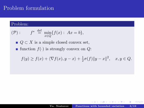
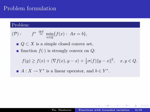
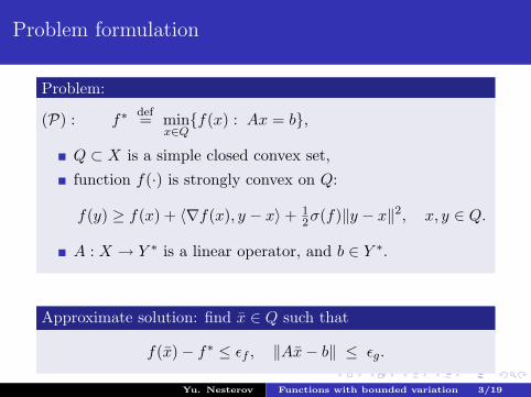


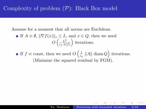

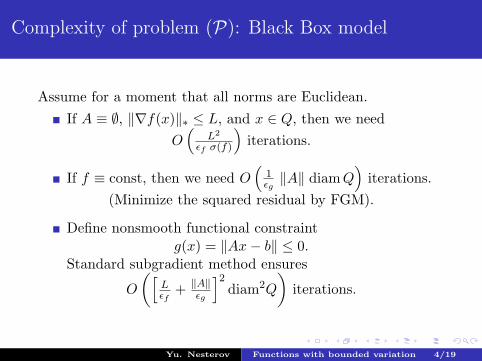


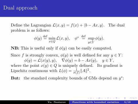
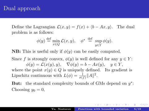
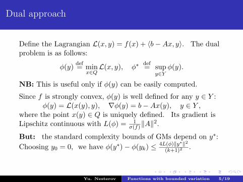


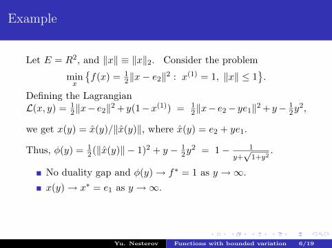
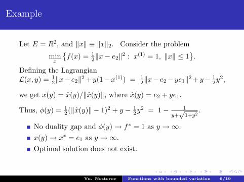


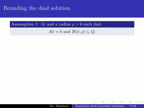
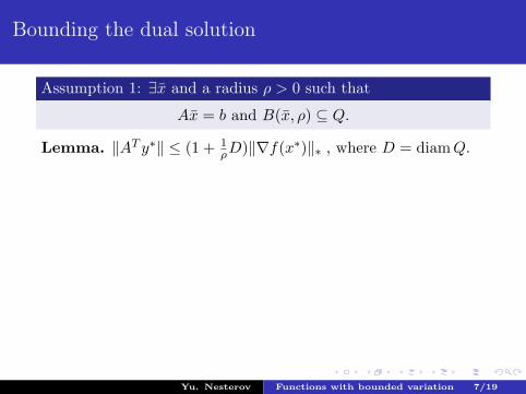
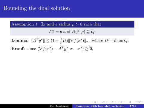
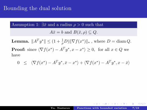


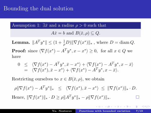


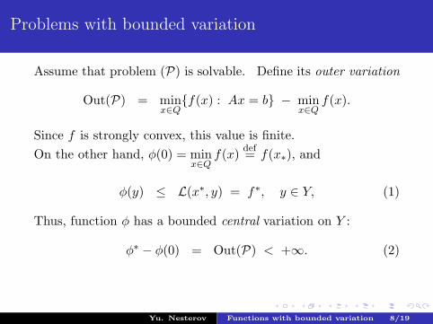


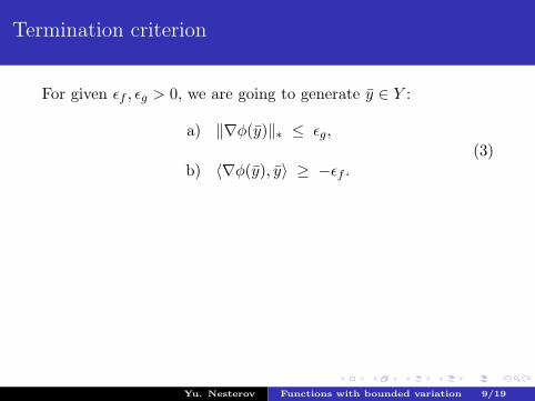
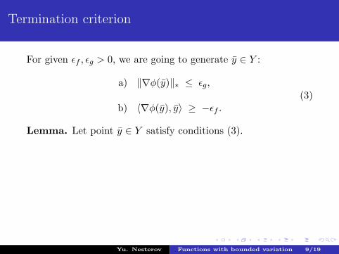
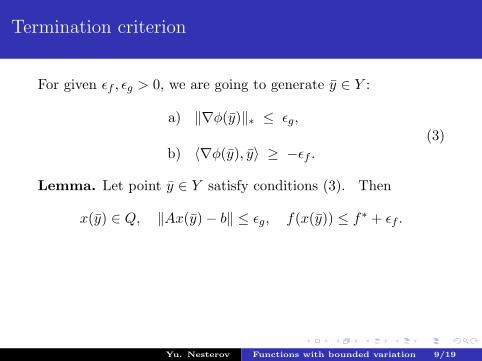
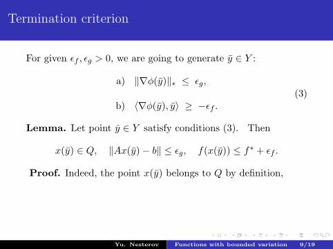
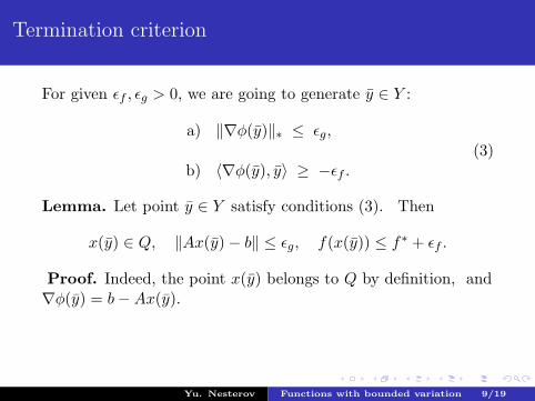
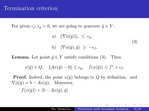

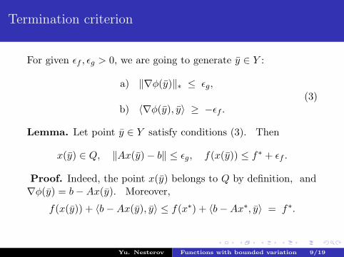
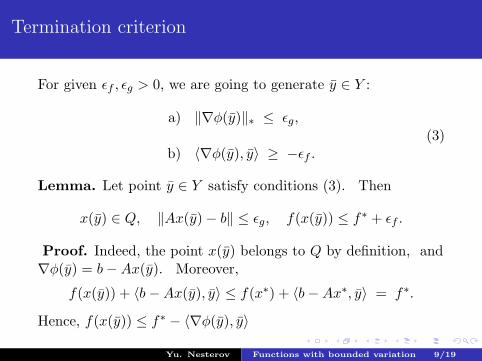
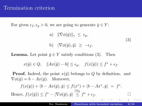

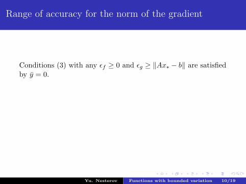

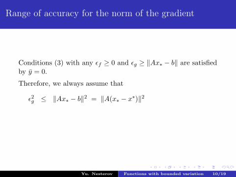
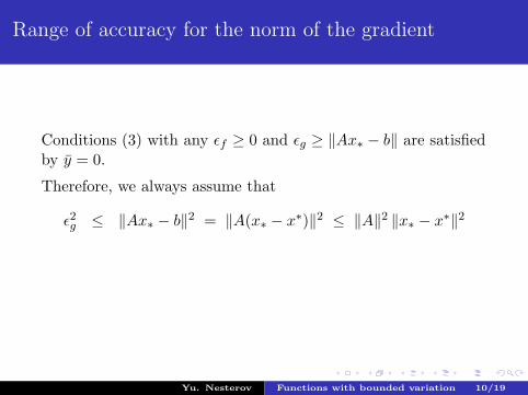

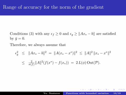


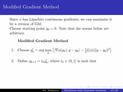


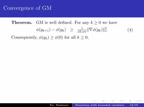
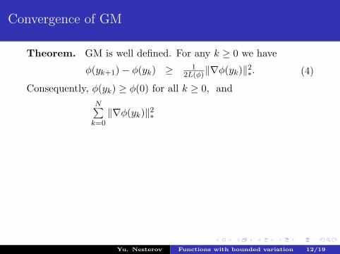
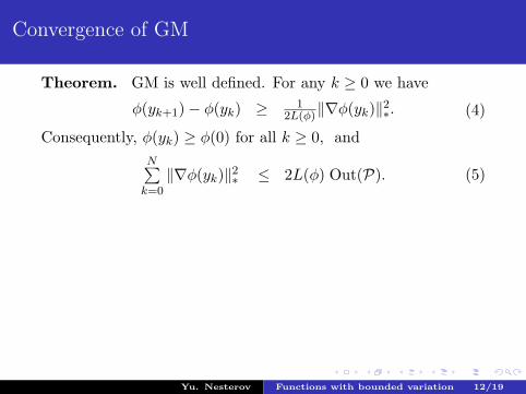

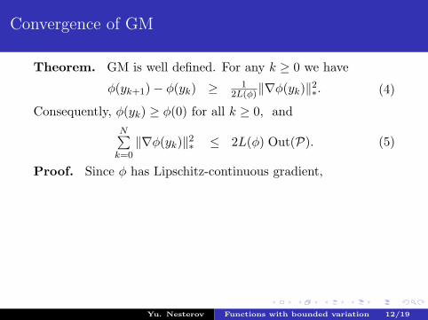
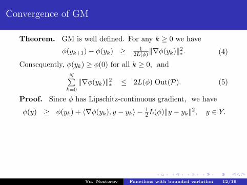

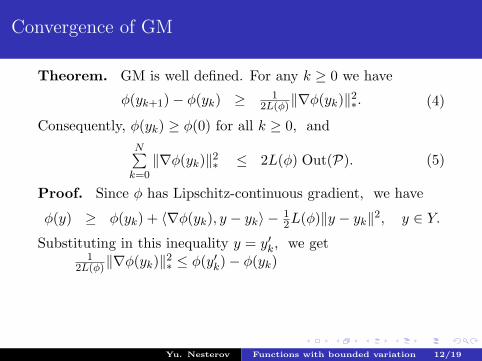
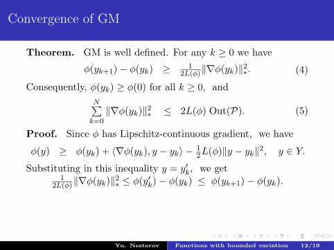


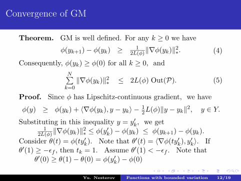
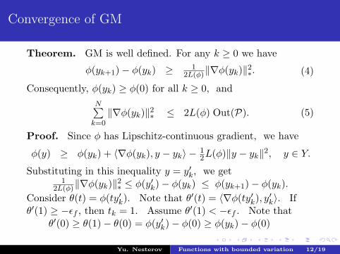


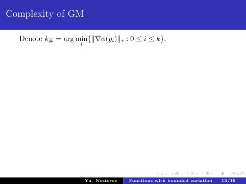
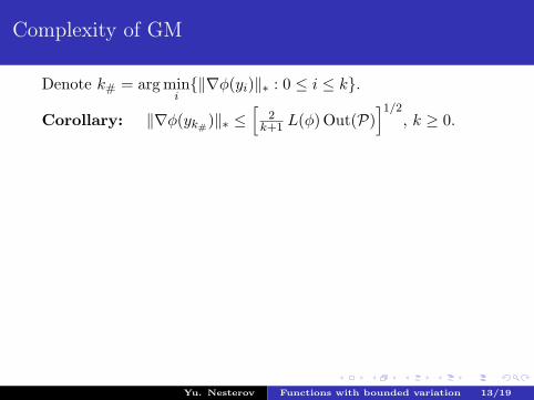
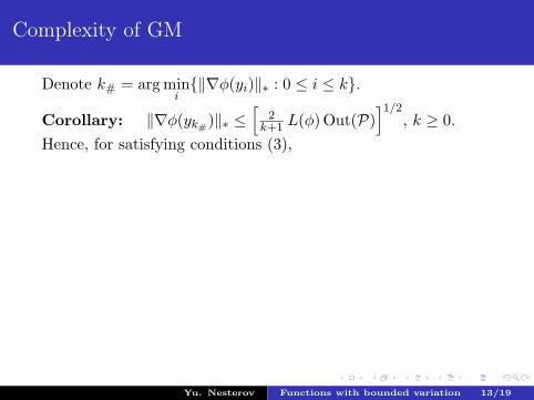
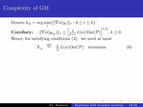


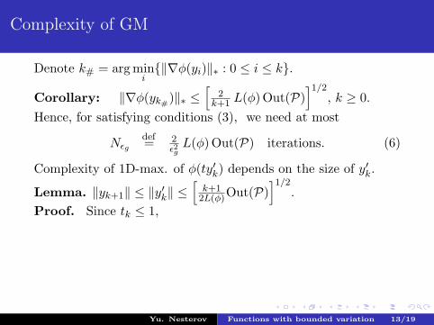
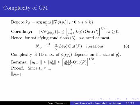

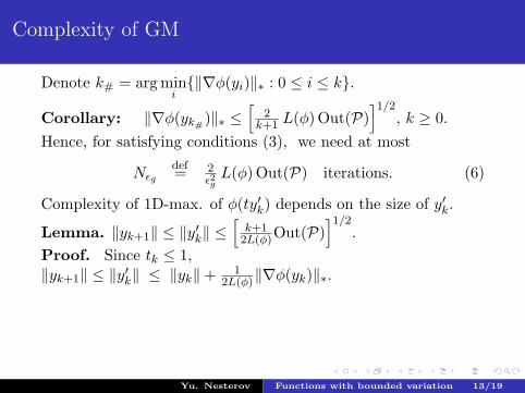
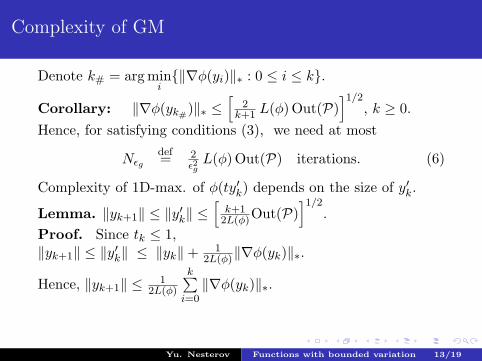
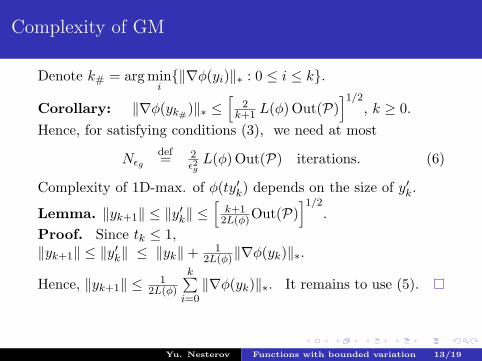

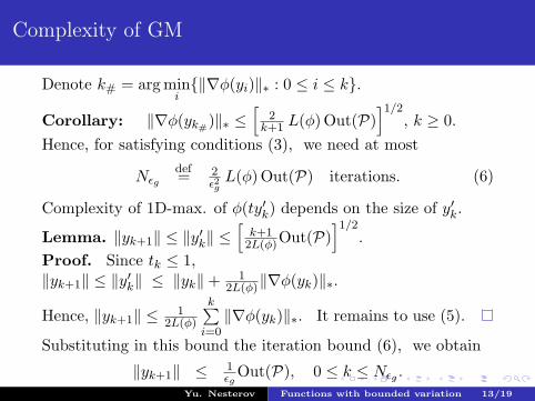


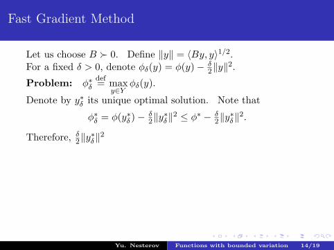

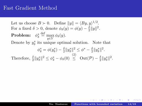

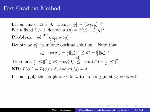


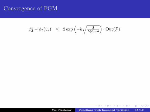
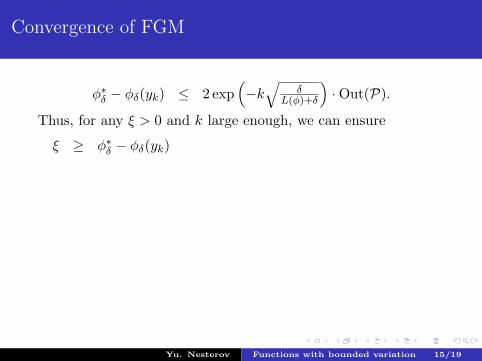
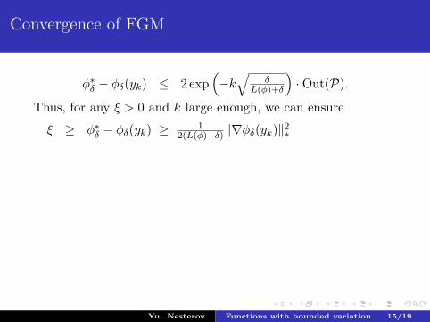
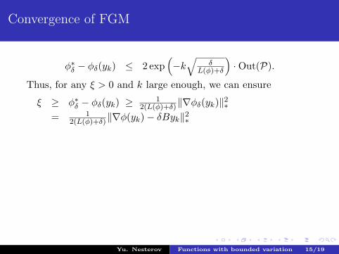


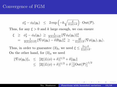
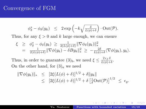
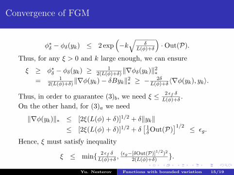


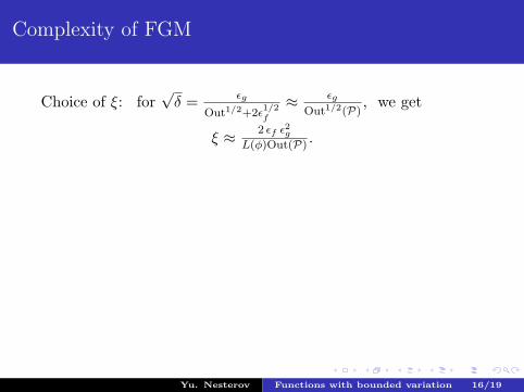
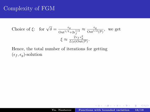


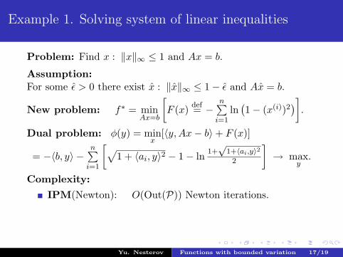

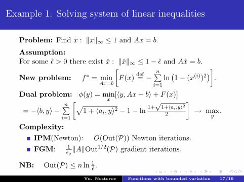


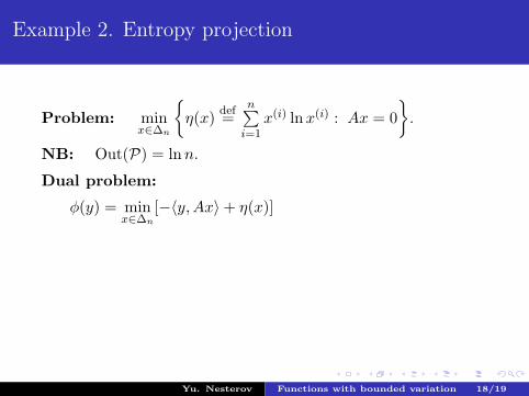


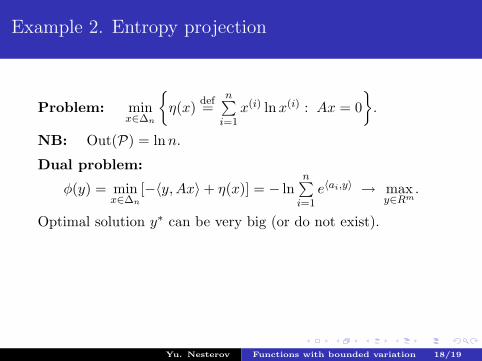


![On Fourier series and functions of bounded variationrspa.royalsocietypublishing.org/content/royprsa/88/606/561.full.pdf · 1913.] Series and Functions of Bounded Variation. 563 the](https://static.documents.pub/doc/80x56/5b0740317f8b9ad5548e0caa/on-fourier-series-and-functions-of-bounded-series-and-functions-of-bounded-variation.jpg)


![CHARACTERIZATIONS OF SIGNED MEASURES IN …torres/pubs/Measures-dual-BV.pdfof BV, the space of functions of bounded variation. Meyers and Ziemer characterized in [19] the Meyers and](https://static.documents.pub/doc/80x56/5b0746707f8b9abf568e40fc/characterizations-of-signed-measures-in-torrespubsmeasures-dual-bvpdfof-bv-the.jpg)


