125
• • •
Durham E-Theses
Three-dimensional Seismic Analysis and Modelling of
Marine Hydrate Systems O�shore of Mauritania
LI, ANG
How to cite:
LI, ANG (2017) Three-dimensional Seismic Analysis and Modelling of Marine Hydrate Systems O�shore of
Mauritania, Durham theses, Durham University. Available at Durham E-Theses Online:http://etheses.dur.ac.uk/12211/
Use policy
The full-text may be used and/or reproduced, and given to third parties in any format or medium, without prior permission orcharge, for personal research or study, educational, or not-for-pro�t purposes provided that:
• a full bibliographic reference is made to the original source
• a link is made to the metadata record in Durham E-Theses
• the full-text is not changed in any way
The full-text must not be sold in any format or medium without the formal permission of the copyright holders.
Please consult the full Durham E-Theses policy for further details.

Academic Support O�ce, Durham University, University O�ce, Old Elvet, Durham DH1 3HPe-mail: [email protected] Tel: +44 0191 334 6107
http://etheses.dur.ac.uk
2

Three-dimensional Seismic Analysis and Modelling of Marine Hydrate
Systems Offshore of Mauritania
Ang Li
A thesis submitted for the degree of
Doctor of Philosophy (Ph.D.) at Durham University
Department of Earth Sciences
Durham University
April 2017

1
Contents Abstracts ....................................................................................................................................... 1
List of Figures ............................................................................................................................... 2
List of Abbreviations .................................................................................................................... 6
Declaration .................................................................................................................................... 7
Acknowledgements ....................................................................................................................... 8
Chapter 1 Introduction .................................................................................................................. 9
1.1 Background ................................................................................................................... 9
1.1.1 Gas hydrate..................................................................................................... 9
1.1.2 Detecting marine hydrate in the subsurface ................................................. 11
1.1.3 Significance of marine hydrate .................................................................... 12
1.1.4 Fluid escape pipes ........................................................................................ 14
1.2 Scope of thesis ............................................................................................................ 15
1.3 Thesis structure ........................................................................................................... 16
1.4 Figures ........................................................................................................................ 18
Chapter 2 Geological Setting, Seismic Dataset and Methodology ............................................. 20
2.1 Geological setting ....................................................................................................... 20
2.2 Seismic dataset............................................................................................................ 21
2.2.1 Acquisition and processing of marine seismic dataset ................................. 21
2.2.2 Seismic dataset and attributes ...................................................................... 22
2.3 Figures ........................................................................................................................ 27
Chapter 3 Gas Trapped below Hydrate as a Primer for Submarine Slope Failures .................... 30
3.1 Introduction ................................................................................................................ 31
3.2 Geological setting ....................................................................................................... 32
3.3 Seismic dataset and methodology ............................................................................... 32
3.4 Observations ............................................................................................................... 33
3.4.1 Seismic pipes ................................................................................................ 33
3.4.2 Architecture of the shear zone ...................................................................... 34
3.5 Interpretations ............................................................................................................. 36
3.5.1 Hydrate-capped gas accumulation ............................................................... 36
3.5.2 Paleo-gas accumulation prior to the failure .................................................. 37
3.6 Discussion ................................................................................................................... 38
3.6.1 Buoyancy and its effect ................................................................................ 38
3.6.2 Preserved overpressure ................................................................................. 39
3.6.3 Dissociation-related failure mechanism ....................................................... 40
3.7 Conclusions ................................................................................................................ 41
3.8 Figures ........................................................................................................................ 42
Chapter 4 Methane Hydrate Recycling probably after the Last Glacial Maximum .................... 50
4.1 Introduction ................................................................................................................ 51
4.2 Geological setting ....................................................................................................... 52
4.3 Seismic data and methodology ................................................................................... 53
4.4 Observations ............................................................................................................... 53
4.4.1 Seabed and BSR ........................................................................................... 53
2
4.4.2 Seismic chimneys and high-amplitude anomalies ........................................ 54
4.5 Interpretation............................................................................................................... 55
4.5.1 Gas trapped below the BSR ......................................................................... 55
4.5.2 Hydrate deposits ........................................................................................... 56
4.6 Discussion ................................................................................................................... 57
4.6.1 Methane passing through the HSZ ............................................................... 57
4.6.2 Model ........................................................................................................... 58
4.6.3 Implications .................................................................................................. 59
4.7 Conclusions ................................................................................................................ 60
4.8 Figures ........................................................................................................................ 61
Chapter 5 Gas venting that bypasses the feather edge of marine hydrate, offshore Mauritania . 66
5.1 Introduction ................................................................................................................ 67
5.2 Gas hydrate and feather edge ...................................................................................... 68
5.3 Geological setting ....................................................................................................... 68
5.4 Seismic dataset and methodology ............................................................................... 69
5.5 Observations ............................................................................................................... 69
5.5.1 Fault system and seabed morphology .......................................................... 69
5.5.2 BSR and diapir ............................................................................................. 70
5.5.3 Positive high amplitude anomalies in levees ................................................ 71
5.6 Interpretation............................................................................................................... 72
5.6.1 Gas venting................................................................................................... 72
5.6.2 Gases trapped below the BSR ...................................................................... 73
5.6.3 Hydrates hosted in levee sediment ............................................................... 73
5.7 Discussion ................................................................................................................... 74
5.7.1 BSR doming ................................................................................................. 74
5.7.2 Implication ................................................................................................... 75
5.8 Conclusions ................................................................................................................ 76
5.9 Figures ........................................................................................................................ 77
Chapter 6 Discussion and Conclusions ....................................................................................... 83
6.1 Uncertainties ............................................................................................................... 83
6.1.1 Seismic resolution and interpretation ........................................................... 83
6.1.2 Resetting of the BHSZ ................................................................................. 84
6.1.3 Parameters in modelling ............................................................................... 84
6.2 Discussion: responses of hydrates to changes in ambient conditions and fate of
released gas ................................................................................................................ 85
6.3 Future work ................................................................................................................. 88
6.4 Conclusions ................................................................................................................ 89
6.5 Figures ........................................................................................................................ 91
References ................................................................................................................................... 93
Appendix 1: Water temperature ................................................................................................ 109
Appendix 2: Two-dimensional heat diffusion model for the BHSZ shift ................................. 110
Appendix 3: One-dimensional synthetic seismogram............................................................... 114
Appendix 4: Horizon maps ....................................................................................................... 116
Appendix 5: Seismic header for block C-19 ............................................................................. 120

1
Abstracts
Marine hydrates, which lock-up vast quantities of methane, are considered to be a
prospective alternative energy source, a slow tipping point in the global carbon cycle and a
probable trigger for submarine failures. In this thesis marine hydrate systems offshore of
Mauritania and associated structural and sedimentary features are investigated by utilising two
surveys of high-quality three-dimensional (3-D) seismic data. Interpreting them provides new
insights into marine hydrate systems and how they respond to changes in ambient conditions.
In one region of one of the 3-D seismic surveys, a shear zone covering 50 km2 is
identified immediately above the hydrate bottom simulating reflector (BSR). It is considered to
be the initial stages of a failure that did not result in widescale downslope transport of the
succession. Due to this failure not going to completion, some free gas remains trapped at the
level of the BSR. At this level the presence of free gases is supported by the continuous high-
amplitude reflections. It is proposed that buoyancy built up by the inter-connected gas
accumulation increases the pore pressure of the overlying hydrate-bearing to the level such that
its base was critically stressed. In this research there is no seismic evidence for failures triggered
by hydrate dissociation but the role of free gas in priming submarine failures is examined.
Whether marine hydrates can release significant amounts of methane into the
atmosphere is inconclusive. In this research a proposed model indicates that methane was re-
captured in the hydrate stability zone after being liberated. Ocean warming since the last glacial
maximum (LGM) gave rise to the shoaling of the base of the hydrate stability zone (HSZ).
Gases released from hydrate accumulating at the base entered the HSZ, driven by buoyancy
built up in the gas accumulation. The hydrate seal was breached and this is manifested by 15 gas
chimneys in seismic data. Hydrates then re-formed at a specific level within the HSZ. This
study implies that not all of methane would enter the ocean after released from hydrates and
therefore the contribution of marine hydrates to the atmospheric methane budget may be not that
much as it was predicted before.
Gas venting is an effective way to transport methane at depth vertically to the ocean and
an example of it is found in the feather edge of marine hydrate. This venting was possible due to
the presence of faults above a salt diapir and is manifested by a series of pockmarks and mounds
at the seabed. The BSR at this site is convex upwards and hence formed a trapping geometry for
underlying free gases. Numerical model shows that this up-convex geometry is caused by the
salt diapir having a higher thermal conductivity. Permeable migration conduits along the faults
and excess pore pressure at the top of the trap allow for the happening of the venting. Compared
with the neighbouring area where the BSR can be well observed, the region affected by
diapirism has a limited scale of the observable BSR. This absence is proposed to result from the
formed trap intercepting methane-rich pore fluid that would migrate landwards along the level
of the base of the HSZ.
2
List of Figures
Fig.1.1 (a) Schematic diagram showing the relationship of phases between dissolved gas, free
gas and gas hydrate (after Davie and Buffett, 2003, their figure 2). Two mechanisms of
formation of gas hydrate: (1) Saturated methane-bearing fluid to form hydrate as it
migrates upwards into the HSZ; (2) Methane concentration is increased by microbial
production of methane until its solubility is exceeded and hydrate forms. (b) T-D
diagram showing the HSZ. HSC –hydrate stability curve, SB – seabed, TP –
temperature profile, HSZ – hydrate stability zone, FGZ – free gas zone. ..................... 18
Fig.1.2 Schematic showing modes of hydrate accumulation at continental slope (after Beaudoin
et al., 2014, their figure 2.1). The figure is not to scale but the width of the section is
likely to be tens to hundreds of kilometres and the depth is probably < 2 km. A, B, C, E
and F are core photos and the width is 7 – 10 cm. D is a photo taken at the seabed. .... 18
Fig.1.3 Seismic expressions of gas chimneys in cross sections. These exampes are from: (a)
offshore Namibia (Moss and Cartwright, 2010); (b) offshore Nigeria (Løseth et al.,
2011) ; (c) offshore mid-Norway (Hustoft et al., 2010); (d) Faeroe-Shetland Basin
(Cartwright, 2007); (e) offshore Mauritania (Davies and Clarke, 2010); (f) offshore
Angola (Andresen et al., 2011); (g) South China Sea (Sun et al., 2013); (h) East Japan
Sea (Horozal et al., 2017) and (i) offshore Norway (Plaza-Faverola et al., 2011). ........ 19
Fig.2.1 Bathymetric map showing the locations of the seismic surveys of C-6 and C-19 (after
Krastel et al., 2006, their figure 3) ................................................................................. 27
Fig.2.2 The schematic figure of the data-acquisition gear. It is based on the information of the
seismic header recorded in the C-19 seismic survey. As the boat sails along, the blue
and the red air gun in turns fire. The blue and red lines are the subsurface lines
corresponding to the blue and the red air gun when activated, respectively. Modified
from Fig.2.6 by Bacon et al., 2007. ............................................................................... 27
Fig.2.3 Typical processing flow chart (Sheriff and Geldart, 1995, their figure 9.62). The steps
marked by (1) to (8) are introduced in the text. ............................................................. 28
Fig.2.4 Zero-phase and minimum-phase wavelet (from
http://wiki.aapg.org/Amplitude_(seismic)). ................................................................... 29
Fig.2.5 Standard polarity. Modified from Sheriff and Geldart, 1995. NP – normal polarity, RP –
reversed polarity, RC+ – positive reflection coefficient. ............................................... 29
Fig.2.6 Seabed reflection and the phase wavelet in seismic surveys of C-6 and C-19. .............. 29
Fig.3.1 (a) Extent of the area covered by the 3-D seismic dataset and its location in relation to
the bathymetry of the continental margin. (b) Dip magnitude map of the seabed
revealing the main sedimentary features at the seabed. The yellow box shows the
location of the study area. (c) Outline of the incompletely developed failure. The
present BSR (its depth is marked in color map) is spatially sub-parallel to the seafloor
(contours indicated by dashed lines, TWTT in seconds). .............................................. 42
Fig.3.2 (a-d) Seismic features of typical pipes. The orientations of these seismic cross sections
are not shown here. (e) Dip magnitude map of BSR, showing the location of pipes
terminating at or below the BSR (marked in yellow circle) and bypassing the hydrate-
containing sediment (marked in red circle). Note that no pipes penetrate the BSR in the
area of the shear zone. The dashed white line marked the area of the shear zone. ........ 43
Fig.3.3 (a) A representative seismic cross section (orientation marked in Fig. 3.1c) showing the
architecture of the shear zone. Note that a seismic pipe terminates at the BSR. UB –
upper boundary, LB – lower boundary, TWTT – two way travel time. (b)(d) Zoomed-in
images exhibiting features at the up-dip (Fig.b) and down-dip (Fig.d) end. (c)(e) RMS
amplitude map of the lower boundary displaying features at the up-dip (Fig.c) and
down-dip (Fig.e) end. ..................................................................................................... 44

3
Fig.3.4 (a) A representative seismic line (orientation marked in Fig.3.1c) showing the
architecture of the shear zone. (b)(c) RMS amplitude map of the lower boundary
exhibiting its planform features. (d) Dip magnitude map of the lower boundary. Note
the ridges occur both on the amplitude map and dip-magnitude map. .......................... 45
Fig.3.5 (a) RMS amplitude map of the present BSR, showing three areas with high seismic
amplitude (named HA1, HA2 and HA3). The western end of HA1 is stratigraphically
linked to the top of pipe clusters. Part of HA3 stays outside the shear zone and is
interpreted as gas leakage. SZ – shear zone. (b-d) Seismic sections displaying high
amplitude reflections within three high-amplitude areas. The ‘band’ is a seismic feature
of the BSR, describing its geometry of high-amplitude section in planform. It is further
discussed in section 5. PR – phase reversal. .................................................................. 46
Fig.3.6 (a) RMS amplitude map of BSR showing a series of high amplitude bands surrounding
the southern margin of the shear zone. (b) Schematic model of how high amplitude
band formed. Reflection X represents a porous bed cross-cut by the BSR. AI – acoustic
impedance. FGZ – free gas zone. (c) Seismic section showing the relationship between
BSR and bands. Where strata is cross-cut by the BSR is commonly marked by seismic
phase reversal. HA – high amplitude, PR – phase reversal. (d) Line drawing of figure c.
The phase reversal is the result of the thin porous beds containing hydrates above the
BSR and gases below it.................................................................................................. 47
Fig.3.7 (a) Seismic cross section showing the inferred original gas column. Its extent is defined
by the continuous high-amplitude reflections with seafloor-reversed polarity. (b) An
RMS amplitude map of the BSR showing the possbile extent of the pre-failure gas
accumulation. (c) Depth-pressure plot showing the buoyancy provided by the inferred
gas column below the failure could reduce the effective stress to the degree that shear
stress exceeds the shear strength. SB – seabed, TA – top of accumulation, BA – bottom
of accumulation, LP – lithostatic pressure, HP – hydrostatic pressure, ES – effective
stress............................................................................................................................... 48
Fig.3.8 The schematic diagram of the buoyancy-related failure mechanism. The gas accumulates
under the hydrate (marked by the BSR) and forms a 263 m-high gas column. It primes
the overlying sediment hosting hydrate, where no pipes develop. The critical height of
the gas column is ~231 m. When the shear stress is less than the shear strength, the
failure plane is under-primed. HP – hydrostatic pressure, LP – lithostatic pressure, TA –
top of accumulation, BA – bottom of accumulation, GA – gas accumulation, RT – roof
thrust, FT – floor thrust. ................................................................................................. 49
Fig.4.1 (a) Location of the 3-D seismic survey. (b) Bathymetric map showing the morphology
of the seabed. Red box – study area. PM – pockmark. (c) The RMS amplitude map of
the BSR in the study area. Red dashed line marks the landward extent of BSR and black
dashed lines represent isobaths. The seismic features of bands (B) are interpreted in
section 5.1. C – canyon, HA – high amplitude, LA – low amplitude in this and
subsequent figures. ......................................................................................................... 61
Fig.4.2 (a) A representative seismic section showing the typical features of a BSR and the gas
accumulations sealed beneath it. B-r-b and r-b-r refer to the black-red-black and red-
black-red seismic loop, respectively. (b) The RMS amplitude map of the BSR
displaying three strike-parallel high amplitude bands (marked by I, II and III). (c)
Interpretation of the cross section X-X’. At the seaward edge of the band feature, phase
reversal sometimes can be seen. The grey colour represents a set of porous thin beds
interbedded with less porous ones. The brighter red and yellow colours mark the higher
saturation of hydrate and gas, respectively. PR – phase reversal. .................................. 62
Fig.4.3 (a) Dip magnitude map of the reflection D. It is marked in Fig.c. In plan view the
positive relief of the chimney is marked in the darker colour. (b) A seismic section
revealing the spatial location of some seismic chimneys. They are marked by the black
box. We use another colour scheme to highlight the seismic polarity of reflections of the

4
seabed (B’) and D (A’). PHAA – positive high amplitude anomalies, FGZ – free gas
zone. (c) Inset of chimney 7. Six reflections (named as A–F) are picked to describe the
amplitude variation around gas chimney and the result is shown in Fig.4.4. PM –
pockmark. ...................................................................................................................... 63
Fig.4.4 RMS amplitude map of the reflections A–F and the BSR (on the left). Their depths are
marked in Fig. 3c. Vertical black dotted lines indicate the spatial location of chimneys 7,
8, 10 and 12. PHAAs at the reflection D and E (outlined by white dashed line) are
identical and interpreted as hydrate deposits. Note that the amplitude values in the
reflection A (the seabed) are very high and its colour scheme is different from others.
The selected examples of the PHAAs are zoomed in (on the right). ............................. 64
Fig.4.5 The modelling result of the BHSZ depth varying with time since the LGM. The
snapshots at three timings (t1-t3) show how the hydrate deposit formed. The red triangle
marks the location where the depth of the BHSZ is modelled in appendix 2. ............... 65
Fig.5.1 Extent of the area covered by the 3-D seismic survey and the location of the study area.
The blue box of solid lines marks where the relatively complete feather edge was
described by Davies et al. (2015). (b) Dip-magnitude map of the seabed in the study
area showing the fault scarp and some reliefs (named as I, II, III and IV). FS – fault
scarp. There are some linear features caused by acquisition noise and they are parallel to
the inline direction. (c) 3-D imaging of the faults (named as F1–13) from top view. The
white arrows mark the displacement direction of the hanging wall. Please note not all
the faults terminate at the seabed. (d) A representative seismic cross section showing the
pattern of the faults and their spatial relationship between the underlying salt diapir. .. 77
Fig.5.2 (a–b) Representative seismic cross sections displaying the spatial relationship between
the reliefs at the seabed, the faults and the salt diapir. The acoustic wiping-out (AWO)
shows up below I-IV and in the zone bounded by F1, F2 and F4. (c–f) Zoom-in figures
showing the cross-sectional geometry of I-IV. (g-j) 3-D imaging of the bathymetry
exhibiting the morphology of I-IV. ................................................................................ 78
Fig.5.3 (a) A seismic cross section showing the upwarping section of the BSR. A different
colour scheme is used to highlight its polarity (cyan-yellow loop) that is opposite to that
of the seabed reflection (yellow-cyan loop). A flat spot is found under the upwarping
BSR. Please note that this figure is exaggerated vertically. HA – high amplitude, LA –
low amplitude in this and subsequent figures. (b) RMS amplitude map of the BSR. The
white lines are the contours of the vertical distance (measured in ms, TWTT) between
the BSR and surface A. Surface A is an assumed planar surface and on each cross line
(E-W oriented) it is a segment defined by the down-dip (1, marked in inset) and the up-
dip point (2) along the BSR. The yellow dashed lines mark the outline of a buried old
canyon and it is described in section 5.6.3. .................................................................... 79
Fig.5.4 (a) Seismic cross section displaying the vertical stacking pattern of the multistory
channel-levee systems. Reflection H, which is interpreted as the levee sediment hosting
hydrates, downlaps upon a paleo-seabed G. (b) Map showing the depth of the paleo-
seabed G. The place in where the old channel diverges is not clearly shown by the
seismic dataset. (c) A seismic cross section showing the spatial relationship between the
BSR and the reflection H. (d) RMS amplitude map of the reflection H. Some positive
high amplitude anomalies (PHAAs) show up at both sides of the buried canyon. ........ 80
Fig.5.5 Modelling result of 2-D heat conduction. The black dashed line marks the top of the
diapir. The blue numbers indicate the temperature of each isothermal line. The black
arrows mark the places where there are some minor discrepancies between the modelled
BSR and the observation result. ..................................................................................... 81
Fig.5.6 (a) The BSR depth measured in two-way travel time (TWTT). No-data places (black
colour) indicate where the BSR cannot be observed in the seismic cross section. (b, c)
Two representative seismic sections showing that BSR can be tracked above the studied
diapir, but is absent elsewhere except the region to the southeast of it. (d) Schematic

5
diagram showing gas migration and where the BSR is present. Black arrows mark the
displacement direction of the hanging wall. The dimension of the diapir and the levee is
not to scale. PM – pockmark, M – mound, GC – gas concentration, HC – hydrate
concentration, GM – gas migration. .............................................................................. 82
Fig.6.1 The 2-D heat conduction modelling results of the BHSZ at present and the LGM. The
upper figure shows the distance between the two modelled BHSZs. The vertical dashed
line marks the position where 2-D heat diffusion model is adopted in chapter 4. ......... 91
Fig.6.2 Methane densities at different depths. They are calculated using Clapeyron equation and
Peng-Robinson equation of state. .................................................................................. 91
Fig. 6.3 Generic diagram showing the marine hydrate system offshore of Mauritania (not to
scale). ............................................................................................................................. 92
Fig.A1.1 Location of sampling of ocean temperature data and the seismic surveys. ............... 109
Fig.A1.2 Temperature-Depth(T-D) profiles of seismic surveys of C-6 and C-19 .................... 109
Fig.A2.1 The modelled locations of the BHSZ with inputs of different geothermal gradient on a
seismic cross section. Their correlation with the observed BSR determines the
geothermal gradient. The inset is the temperature-depth plot of the ocean water. ...... 113
Fig.A2.2 The variation of relative sea level (RSL) (a) and bottom water temperature (BWT) (b)
in the last 20 kyr. The modelled variation of the BHSZ depth is shown in Fig. c. The
site is marked by the red triangle in Fig. 4.5. A gas chimney is observed here. mbsf –
metres below seafloor. ................................................................................................. 113
Fig.A3.1 (a) Model of the isolated hydrate reservoir and (b) model of the hydrate deposit
underlain by free gas zone. Medium 1 is clay, medium 2 is hydrate-containing sandy
sediment and medium 3 is gas-charged sediment. The black arrows mark the interface
between clay and hydrate-bearing sandy sediments. The red arrow indicates the location
of the BSR. ................................................................................................................... 114
Fig.A3.2 Synthetic seismic diagram of model a. Porosities of hydrate reservoir and clay are 30%
and 20%. HC – hydrate concentration, RC – reflection coefficient for this and
subsequent figures. ....................................................................................................... 115
Fig.A3.3 Synthetic seismic diagram of model a. Porosities of hydrate reservoir and clay are 40%
and 20%. ...................................................................................................................... 115
Fig.A3.4 Synthetic seismic diagram for the interface between hydrate-containing and gas-
charged sediments (model b). ...................................................................................... 115
Fig.A4.1.A – dip magnitude map of seabed; B – RMS amplitude map of BSR; C – RMS
amplitude map of top of shear zone; D – RMS amplitude map of base of shear zone; E –
RMS amplitude map of reflection FGZ1; F – RMS amplitude map of reflection FGZ2;
G – RMS amplitude map of reflection FGZ3 .............................................................. 116
Fig. A4.2 A representative seismic cross section of block C-6. Its location is shown in
Fig.A4.1.Please note the vertical exaggeration of the inset of the gas chimney is 1. .. 117
Fig.A4.3 A – dip magnitude map of seabed; B – RMS amplitude map of seabed; C – RMS
amplitude map of BSR; D – RMS amplitude map of reflection D. Reflections of A, B, C,
E and F are stated in chapter 4. .................................................................................... 118
Fig. A4.4 A representative seismic cross section of block C-19. Its location is shown in
Fig.A4.3. ...................................................................................................................... 119
6
List of Abbreviations
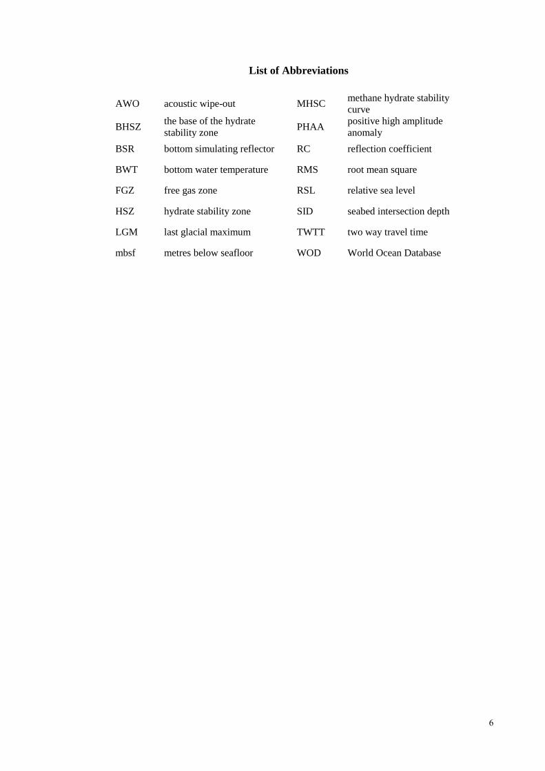
AWO acoustic wipe-out MHSC methane hydrate stability
curve
BHSZ the base of the hydrate
stability zone PHAA
positive high amplitude
anomaly
BSR bottom simulating reflector RC reflection coefficient
BWT bottom water temperature RMS root mean square
FGZ free gas zone RSL relative sea level
HSZ hydrate stability zone SID seabed intersection depth
LGM last glacial maximum TWTT two way travel time
mbsf metres below seafloor WOD World Ocean Database

7
Declaration
I declare that the work presented in this thesis, submitted for the degree of Doctor of
Philosophy at Durham University, is entirely my own except where clearly stated. To the best of
my knowledge, this thesis is distinct from any previously submitted or published at this or any
other university.
Ang Li
Department of Earth Sciences
Durham University
January 2017
©The copyright of this thesis rests with the author. No quotation from it should be published
without the prior written consent and information derived from it should be acknowledged.

8
Acknowledgements
Writing this note of thanks is the finishing touch on my thesis and I am very happy to
see this day coming. Doing the Ph.D. of geology means a lot to me. Here I would like to convey
my heartfelt gratitude to the people who help so much in these four years, not only in the
scientific field but also at a personal level.
First I would like to thank my supervisor Richard J Davies for your professional help.
You always lead me to think critically when facing a scientific question and encourage me to try
some new ideas. This is of great help for me to growing into an independent researcher. I also
would like to thank you for tolerance with my ‘Chin-English’ writing at the beginning of the
research. Your decency, passion and insistency on how to do science impress me and will not be
forgotten in my future career.
I would like to thank my supervisors Richard Hobbs, Simon Mathias and Jonathan
Imber for your wonderful cooperation in my thesis. Your knowledge takes me to different
worlds of geology and extends my skills of solving geological problems. Your office doors are
always open to me and this gives me more confidence to finish the Ph.D. degree.
My reviewers, Neil Goulty, Christine Peirce and Andrew Aplin, are appreciated for
guiding me through the research. Your objective viewpoints and sharp observation push me to
re-evaluate my work and find its uncertainties. Your thought-provoking questions in the annual
reviews allow me to assess the progress of the research by myself and manage the time such that
I can learn how far to go to finish my thesis. I also would like to thank Jon Gluyas and Ken
McCaffrey for their lecturing during the CeREES fieldtrip. Looking at the outcrops allows me
to learn what the true world of petroleum system is like.
I thank Durham University for providing the friendly working environment and my
research funding. I also thank China Scholarship Council (CSC) for providing such an excellent
platform of studying abroad and covering my living costs. David Stevenson and Gary
Wilkinson are thanked for their help in maintaining the hardware and software related to this
research. The computers are moody and not easy to take care of. Hatfield College is thanked for
its financial help in this research.
I would like to thank my colleagues, Jinxiu Yang, Yang Li, Longxun Tang, Sal
Goodarzi, Loraine Pastoriza, Jack Hardwick, Alex Lapadat, Nadia Narayan, Adam Sproson,
Ben Maunder, Harisma Andikagumi, Lamees Abdulkareem, Oliva Sanford, Dimitris
Micheliousdakis, Charlotte Withers, Francesca E. Watson, Xiang Ge, Zeyang Liu, Huifei Tao,
Wei Zhou and Meiyan Fu. We support each other by deliberating over our problems and talked
about things other than just our papers. I also would like to thank my housemates, Junjie Liu,
Jing Zhang, Qi Wang, Rongjuan Wang and Yan Qu and my friends, Steve, Yuexian Huang,
Xiaolin Mou, Dan Li, Mengwei Sun, Josh, Allan Roberts and Vishal Bandugula Janardhan.
Chatting with you guys can let me put the work aside temporarily and enjoy the life.
Last but not least, I would like to thank parents for your sympathetic ear. You are
always there for me. Hopefully my small achievement of getting the Ph.D. degree would make
you proud. A big thank to my wife who always supports me and takes care of our new born
daughter Xuan. You never know how much I miss you and this missing is my biggest
motivation to finish my work.

Chapter 1
9
Chapter 1 Introduction
1.1 Background
1.1.1 Gas hydrate
Marine hydrates are ice-like crystalline solids in which gas is physically trapped by
water molecules in clathrates (Sloan and Koh, 2007). Gas hydrates have three crystal structures
– cubic structure I (sI) (McMullan and Jeffrey, 1965), cubic structure II (sII) (Mak and
McMullan, 1965) or hexagonal structure H (sH) (Ripmeester et al., 1987). Most of the gas
hosted in marine hydrate is methane and this is a potent green-house gas (Houghton et al., 1992).
Its proportion relative to other gases can be up to 99% and the remaining gas includes but is not
limited to ethane, propane and carbon dioxide (Soloviev and Ginsburg, 1994). The chemical
compound for methane hydrate is CH4•nH2O and for structure I, n = 5.75 (Sloan and Koh, 2007).
The process of hydration is an exothermic reaction that takes place under low
temperature and high pressure (Sloan and Koh, 2007). In a temperature-pressure (P-T) plot the
concave-down curve representing the phase boundary between gas and hydrate is the hydrate
stability curve (HSC) which has been measured in the laboratory (Moridis, 2002; Lu and Sultan,
2008). Given that the concentration of the dissolved methane exceeds its solubility, hydrate
would be stable under some P-T conditions (Fig. 1.1) and these can be met in deep marine
environments and the regions where permafrost forms (Kvenvolden, 1993). The zone where
hydrate is stable is termed the hydrate stability zone (HSZ) and it can theoretically extend from
above the seabed to hundreds of metres below it. Once hydrate has formed in the water column,
its buoyancy will raise it to the level at where it is no longer stable, so marine hydrates are
normally stable in the HSZ below the seabed (Sloan and Koh, 2007; Fig. 1b). The critical water
depth at which methane hydrate is stable in high latitude zones of the Arctic and Antarctic is
shallower than that near the equator (Archer et al., 2009). Apart from P-T conditions, other
factors that control the stability of hydrate include salinity and gas composition (Sloan and Koh,
2007). A hypersaline environment is an inhibitor for hydrate formation (Liu and Flemings, 2006;

Chapter 1
10
Sloan and Koh, 2007). Localised hypersaline environments may be a mechanism for gas passing
through the hydrate stability zone (HSZ), which has been recorded by measuring levels of
chloride offshore of Oregon (Liu and Flemings, 2006). Hydrates with a higher proportion of
heavier hydrocarbon gases have a deeper position for the base of the hydrate stability zone
(BHSZ) (Sloan and Koh, 2007). For instance, in the area of Storegga Slide the BHSZ formed by
92% methane and 8% ethane is 45 m lower than that of hydrate made up of 99% methane and 1%
ethane at the water depth of 880 m (Posewang and Mienert, 1999). Complex gas composition is
thought to give rise to multiple BSRs (Tréhu et al., 1999; Andreassen et al., 2000; Foucher et al.,
2002; Golmshtok and Soloviev, 2006; Popescu et al., 2006), but this explanation is still
questioned (Posewang and Mienert, 1999).
Continental slopes are common sites where marine hydrate accumulates (e.g. the Gulf
of Mexico, Brooks et al., 1984; the Okhotsk Sea, Ginsburg et al., 1993; offshore Costa Rica,
Ruppel and Kinoshita, 2000; the Blake Ridge, Hornbach et al., 2003; at the Storegga slide, Bünz
and Mienert, 2004; offshore Oregon, Tréhu et al., 2004; Hornbach et al., 2008; offshore Alaska,
Collett, 2008; eastern Nankai Trough, Saeki et al., 2008; offshore Svalbard, Bünz et al., 2012;
offshore Angola, Serié et al. 2012). It often accumulates at the BHSZ when dissolved gas is
transported upwards into the HSZ by migrating pore-water and sufficient to create hydrates (Fig.
1.2, Singh et al., 1993; Hornbach et al., 2003; Haacke et al., 2007). Free gas is often below the
BSHZ. It is formed by the hydrate recycling mechanism in which water and gas are released
from hydrate-containing sediments due to the upward shift of the BHSZ, driven by the ongoing
sedimentation, tectonic uplift, sea-level fall or bottom water warming. The FGZ can also be
formed by the solubility-curvature mechanism that states the concentration buffer of gas hydrate
enables the competing effect of downward diffusion and upward advection to form a steady-
state aqueous concentration curve. If this curve and that of the solubility is sufficiently flat, pore
water becomes saturated and free gas can form (Haacke et al., 2007). When gas can coalesce to
form a continuous buoyant volume (gas saturation could be ~10%, Schowalter, 1979), it is
normally trapped below the BHSZ due to the clogging effect of hydrates in sediments (Nimblett

Chapter 1
11
and Ruppel, 2003; Chabert et al., 2011). Gas hydrates can also be found to outcrop at or near the
seabed. The outcropping hydrate-bearing sediments imaged by photos or seismic data have
mound-like morphology, either near the intersection between the BHSZ and the seabed (Egorov
et al., 1999) or kilometres away from this intersection in a seaward direction (Roberts, 2001;
Serié et al. 2012). In addition, gas chimneys, which are interpreted as potential migration
pathways for water and gas to reach the seabed (Cartwright and Santamarina, 2015), could be
favourable places for hydrate accumulations (Fig.1.2, Plaza-Faverola et al., 2010). So far these
are the main patterns of hydrate accumulation that have been seen more than once in different
areas around the world.
1.1.2 Detecting marine hydrate in the subsurface
Hydrate can be identified visually in cores brought to the surface. Direct observation of
the gas hydrate in cores sampled from the deep-water sediments has been recorded in the
Okhotsk Sea for example (Ginsburg et al., 1993). It has been found in veins, nodules or sub-
horizontal layers (Ginsburg et al., 1993; Kvenvolden, 1993). The Pressure Core Sampler (PCS)
tool is used to directly measure the gas released from hydrate under in-situ P-T condition
(Dickens, 1997; Milkov et al., 2004; Yun et al., 2011) and it allows for an assessment of the
amount of methane stored in hydrates in an area of interest. The photos taken by a remote
operated vehicle (ROV) have shown that hydrate mounds exposed at the seabed can be partly or
completely covered by chemosynthetic communities, such as bacterial mats and tube worms
(Hovland and Svensen, 2006; Roberts et al., 2006). During its dissociation, hydrate absorbs heat
and leaves low temperature anomalies in the extracted core (Ford et al., 2003). Therefore, the
temperature profile obtained by scanning using infrared rays can indicate where hydrate
dissociated before (Ford et al., 2003; Tréhu et al., 2004). Other core-scale data that can indicate
the presence of gas hydrate is an anomalously low chloride concentration as hydrate
dissociation releases water and therefore decreases the salinity of pore fluid (Hesse and Harrison,
1981; Tréhu et al., 2004). Hydrate can also be found in the sedimentary succession based on the
analysis of well-logs such as the electrical resistivity log and the acoustic transit-time log

Chapter 1
12
(Collett, 2001). An increase in resistivity and a decrease in transit times indicates the presence
of gas hydrate (Collett, 1999; Collet and Wendlandt, 2000; Lee et al., 1993).
Hydrate can be revealed by seismic imaging. The bottom simulating reflector (BSR) is a
robust indirect proxy for the presence of hydrate (Tréhu et al., 2003). These reflections were
first reported in the 1970s (Shipley et al., 1979) and since then examples have been found along
continental margins (e.g. Tréhu et al., 2006) and in lakes (e.g. Vanneste et al., 2001). The
occurrence of BSRs is a seismic response to the transition from hydrate-bearing sediment to
underlying sediment hosting free gas. Reflections occur even when the saturation of trapped gas
is as low as 1%-5% (MacKay et al., 1994). The BSR shallows landwards until it intersects the
seabed and this zone is termed the feather edge (more introduction please see section 5.2). In the
HSZ an isolated gas hydrate deposit can be detected on the basis of an acoustic impedance
contrast between hydrate-bearing and hydrate-free sediments and it is normally lower than that
at the BHSZ (Zhang et al., 2012). Hydrate concentration can be calculated based on rock
physics models and assumptions regarding whether it is part of the pore fluid or the cementing
sediment grains (e.g. offshore Svalbard, Chabert et al., 2011). Up until now this is the
geophysical approach that has been used most commonly in assessing hydrate resources.
Electromagnetic method is an additional tool to seismic surveys and have the potential to detect
the hydrate and its volume due to its higher electrical resistivity than water-saturated sediments
(Weitemeyer et al., 2006). The concentration of gas hydrate is estimated to be 0-30% and 27-46%
offshore Oregon using this method (Weitemeyer et al., 2006; Weitemeyer et al., 2011).
1.1.3 Significance of marine hydrate
The process of hydration significantly narrows the molecular spacing of gas. This
means hydrate can host gas whose volume under standard temperature and pressure (STP) is
~164 times as that of the hydrate itself (Max et al., 2005). Therefore, hydrate accumulations can
be taken as a concentrated hydrocarbon resource and its prospect of being an energy source has
been recognised (Collett, 2002; Kerr, 2004; Boswell, 2009). To better assess this potential, we
Chapter 1
13
have to know how much methane is trapped in marine hydrate (Kvenvolden, 1993). So far the
error of the estimation of the global hydrate reserves might have orders of magnitude and this
estimate has been updated several times (Kvenvolden, 1988; Gornitz and Fung, 1994; Harvey
and Huang, 1995; Collett, 2002; Milkov, 2004; Johnson, 2011). The latest estimates of the
global resources of methane trapped in hydrate are 4705 – 313992 trillion cubic feet (TCF)
which is 133.2– 8891.3 trillion cubic metres (TCM) (Johnson, 2011). Even if a small proportion
of this gas is exploitable, it exceeds the sum of the known terrestrial reserves of natural gas
(Kerr, 2004). Nowadays methane hydrate as a source of methane is technically feasible
(Boswell, 2009). Developing gas hydrate by means of depressurisation has been tested and the
gas flow is got (Moridis, 2008; Yamamoto et al., 2014).
Gas hydrate has been referred to as a large carbon capacitor that accounts for a
proportion of the potentially releasable carbon in the oceanic lithosphere (Dickens, 2003). The
possibility of methane that is or was hosted in hydrate entering the ocean and atmosphere has
been speculated before (Kennett et al., 2000). Whether this methane has contributed or could
contribute in the future to climatic warming is an important geoscientific question, particularly
because estimated global climatic temperatures closely track methane concentrations in the
atmosphere (Kvenvolden, 1993; Loulergue et al., 2008). The answer, however, is much debated.
Methane liberated from gas hydrate due to oceanic warming and massive methane release have
been predicted (Berndt et al., 2014; Phrampus and Hornbach, 2012), but most of this methane
(~60 %) would be consumed by oxidation in the ocean (Graves et al., 2015) and only modest
quantities are thought to be able to reach the atmosphere. Even so, it can sometimes escape into
the atmosphere through focussed gas venting within gas plumes (Graves et al., 2015; McGinnis
et al., 2006; Myhre et al., 2016). However, Arctic ice records casts doubt as to whether methane
escape from methane hydrates makes a contribution to atmospheric levels during late
Quaternary rapid warming events (Sowers, 2006). Even if methane liberated from marine
hydrate could enter the atmosphere, it is thought this entry would be slow, rather than resulting
in the spike of the methane budget on a human time scale (Archer et al., 2009). Methane release
Chapter 1
14
from hydrates in the Arctic and Subarctic area over the next century is predicted given different
scenarios of future climate and sea level change (Hunter et al., 2013; Vadakkepuliyambatta et
al., 2017) and the impact of this release on climate is under research (Ruppel and Kessler, 2016).
Marine hydrate is considered to have the potential to destabilise marine sediments and
trigger submarine failures that could destroy submarine infrastructure (Kvenvolden, 1993; Lane
and Taylor, 2002). Once hydrate has formed and filled pore space of marine sediments,
consolidation and cementation are inhibited (McIver, 1982). Gas hydrate at the BHSZ is
metastable and will decompose when ambient conditions change (e.g. bottom water temperature
increases or sea level drops). As a result, sediment hosting hydrate may become under-
consolidated and overpressured if dissociation occurs. This primes submarine slides that can be
later triggered by gravitational loading or earthquakes (McIver, 1982). This mechanism may
explain the formation of the Storegga slide offshore of Norway for example, although whether it
is responsible is inconclusive (Berndt et al., 2002; Kvalstad et al., 2005; Mienert et al., 2005;
Brown et al., 2006).
1.1.4 Fluid escape pipes
Fluid escape pipes were defined as a highly localised vertical to sub-vertical pathways
of focused fluid (Carwright and Santamarina, 2015). There are other terms referring to these
features, such as seismic chimneys and gas chimneys that both have a columnar shape and
similar formation mechanisms and seismic features with pipes (Carwright et al., 2007;
Carwright and Santamarina, 2015). Pipes are found in deep-water settings around the world and
their presence suggests that over-pressured pore fluid, which normally carries considerable
amount of gas, bypasses the overlying sediments and potentially enters the ocean (Carwright et
al., 2007). The outcrop of pipe has been found in Greece and show metre-sized cavities at the
bottom, circular tot oval structures in the middle and strongly sheared country rock at the top
(Løseth et al., 2011). Most of the observation of pipes is made in seismic survey. Pipes manifest
as vertical to sub-vertical zones of disrupted reflectivity (Fig. 1.3). The stratal reflections within

Chapter 1
15
these zones may be offset, deformed, attenuated or are enhanced (Fig. 1.3, Carwright and
Santamarina, 2015). The imaging quality of pipes decreases with increasing buried depth and
decreasing pipe width (Løseth et al., 2011; Carwright and Santamarina, 2015). Pipes can form
when (1) a network of hydraulic fractures triggered by excess pore pressure propagates towards
the seabed (Carwright et al., 2007); (2) the fluidised grains of sediment are mobilised by
seepage forces (Carwright et al., 2007; Moss and Cartwright, 2010b); (3) an accumulating gas
column overcomes the capillary sealing and advances as a piston (Cathles et al., 2010); or (4)
localised subsurface volume is lost hence vertical permeability is significantly increased
(McDonnell et al., 2007; Sun et al., 2013).
1.2 Scope of thesis
Marine hydrate system and gas migration in the subsurface offshore of Mauritania have
been documented. The BSR, gas seepages, mud volcanoes and slope failures are identified in
the 2-D seismic survey (Lane and Taylor, 2002). 3-D seismic survey allows for more
knowledge related to the hydrate system, including that gas can migrate along the gravity-driven
faults (Yang and Davies, 2013) and the BHSZ (Davies et al., 2014) and through mass transport
complex (MTC) (Yang et al., 2013). Gas can also be recycled in stratigraphy trap, which can
lead to more gas accumulation and overpressure at its top (Davies and Clarke, 2010). Changes
in bathymetry, such as sedimentation and canyon migration at the seabed, result in the resetting
of the BSHZ (Davies and Clarke, 2010; Davies et al., 2012b). In general the presence of this
widespread resetting is evidenced by tracking the relict bases of marine hydrates in the seismic
dataset (Davies et al., 2012a). This research continues to focus on the marine hydrate system
offshore of Mauritania.
The fundamental question addressed here is how the marine hydrate system responds to
changes in ambient conditions and what the geological results and implications are. Hydrate
dissociation due to bottom water warming has been predicted in high-latitude zones (e.g. Berndt
et al., 2014), but whether this scenario takes place in the low-latitude zones such as offshore of
Chapter 1
16
Mauritania has not been documented. In this research seismic features of the BSR and related to
gas accumulation and migration are described and interpreted. Numerical modelling is used to
estimate the depth of the present-day BHSZ at present and in the past and resetting of the BHSZ
in a setting affected by a salt diapir. The modelling results combined with the interpretations of
two 3-D seismic surveys provide new insights into the marine hydrate system. The link of
marine hydrates to submarine failures, under what circumstances methane is vented and in what
way is methane recycled will be investigated.
1.3 Thesis structure
Chapter 2 starts with the introduction of the geological setting offshore of Mauritania.
This is followed by an explanation of the general workflow for acquisition and processing of the
seismic datasets and the types of seismic attributes used in this research. Chapters 3-5 present
the key results and interpretations in the form of the independent research papers. Each of them
attempts to answer a scientific question so as to extend our knowledge of the marine hydrate
system. The word ‘we’ refers to the authorship denoted in each chapter. Chapter 3 is published
by the journal of Marine Geology. Chapters 4 and 5 are accepted by the journal of Marine and
Petroleum Geology. All the words are written by the writer and revised by the co-authors. The
modelling code is written through collaborating with Simon and Jinxiu. All of the reflections in
this study are picked, tracked and mapped by the writer except the seabed reflection in chapter 3
and the BSR in chapter 5.
The title of chapter 3 is ‘Gas trapped below hydrate as a primer for submarine slope
failures’. 3-D seismic imaging reveals a shear zone at the base of a partially developed slope
failure, immediately above a BSR. This is a rare example of a shear zone that did not lead to the
complete development of a slope failure. It is proposed it provides the first seismic evidence
that the buoyancy effect of gas below the hydrate rather than the hydrate dissociation is also a
viable mechanism for large-scale slope failures.

Chapter 1
17
The title of chapter 4 is ‘Methane hydrate recycling probably after the last glacial
maximum’. Knowing how methane is recycled in marine hydrate system is important in
assessing the contribution of marine hydrate to the carbon budget in the ocean and atmosphere.
This research provides a new evidence of methane recycling by showing some hydrate deposits
that are interpreted to be recycled from gases trapped below the HSZ. The trigger for the
methane transport may be the oceanic warming since the LGM. This process is a mechanism
buffering methane escape towards seafloor and speculated to in part explain why atmospheric
methane in the late Quaternary is not recorded in the ice cores in the polar region.
The title of chapter 5 is ‘Gas venting that bypasses the feather edge of marine hydrate’.
A venting system has been identified based on the spatial relationship between pockmarks and
permeable faults. Methane is interpreted to be vented to the seafloor surface or trapped below
the elongated up-domed BHSZ. The absence of the BSR landward of the venting system
suggests that relatively few gases exist in the locale. Investigation into this venting allows for
analysing the probable impact of venting on landward gas migration.
Chapter 6 discusses the uncertainties encountered throughout the research. They include
uncertainties in seismic resolution, resetting of the BHSZ and input parameters into numerical
models. Future work involves predicting methane release, its fate, what proportion of methane
release would be retained in subsurface and implication for the climate change. The thesis ends
with listing the key findings and the conclusions.

Chapter 1
18
1.4 Figures
Fig.1.1 (a) Schematic diagram showing the relationship of phases between dissolved gas, free gas and gas
hydrate (after Davie and Buffett, 2003, their figure 2). Two mechanisms of formation of gas hydrate: (1)
Saturated methane-bearing fluid to form hydrate as it migrates upwards into the HSZ; (2) Methane
concentration is increased by microbial production of methane until its solubility is exceeded and hydrate
forms. (b) 𝑇-𝐷 diagram showing the HSZ. HSC –hydrate stability curve, SB – seabed, TP – temperature
profile, HSZ – hydrate stability zone, FGZ – free gas zone.
Fig.1.2 Schematic showing modes of hydrate accumulation at continental slope (after Beaudoin et al.,
2014, their figure 2.1). The figure is not to scale but the width of the section is likely to be tens to
hundreds of kilometres and the depth is probably < 2 km. A, B, C, E and F are core photos and the width
is 7 – 10 cm. D is a photo taken at the seabed.

Chapter 1
19
Fig.1.3 Seismic expressions of gas chimneys in cross sections. These exampes are from: (a) offshore
Namibia (Moss and Cartwright, 2010); (b) offshore Nigeria (Løseth et al., 2011) ; (c) offshore mid-
Norway (Hustoft et al., 2010); (d) Faeroe-Shetland Basin (Cartwright, 2007); (e) offshore Mauritania
(Davies and Clarke, 2010); (f) offshore Angola (Andresen et al., 2011); (g) South China Sea (Sun et al.,
2013); (h) East Japan Sea (Horozal et al., 2017) and (i) offshore Norway (Plaza-Faverola et al., 2011).

Chapter 2
20
Chapter 2 Geological Setting, Seismic Dataset and Methodology
2.1 Geological setting
The Northwest African continental margin formed after seafloor spreading which began
in late Triassic to mid-Jurassic times (Rad et al., 1982). After rifting, thick sediment packages
accumulated and at present the sediments deposited in the Senegal-Mauritania Basin are more
than 10 km thick (Rad et al., 1982). The continental shelf offshore Mauritania is typically 25-50
km wide, while in the north it expands to up to 150 km wide and forms the shallow marine
platform of the Banc d’Arguin (Henrich et al., 2010; Zühlsdorff et al., 2007). Some canyons
incise the continental slope such as the Timiris and Tioulit Canyon (Fig. 2.1; Seibold and
Fütterer, 1982; Antobreh and Krastel, 2007). Seismic reflection profile EXPLORA 78-48 along
with the DSDP 367 and 368 constrain the age of the sedimentary rocks offshore of Mauritania
as younger than Jurassic (Rad et al., 1982). The presence of salt diapirs indicates that evaporates
were deposited on the subsiding continental basement blocks in a narrow elongate zone between
16o N and 19
o N (Rad et al., 1982). A prominent sedimentary feature is the Mauritania Slide
Complex that formed as a result of multiple failure events (Antobreh and Krastel, 2007). More
details about the sedimentary setting and the petroleum system will be introduced in the section
of geological settings in chapters 3 to 5.
The studied succession, which extends from the seabed down to ~500 m below it, were
deposited from Pliocene to present day and this age is constrained by the exploration well of
Ras El Baida A-1 (20o15′48″ N, 17
o52′02″
W). Along the continental margin there is strong
seasonal upwelling caused by the interaction between the trade wind system in the northern
hemisphere and the African monsoonal system in a southern direction (Wefer and Fischer, 1993;
Nicholson, 2000).

Chapter 2
21
2.2 Seismic dataset
2.2.1 Acquisition and processing of marine seismic dataset
The author was not involved in the acquisition and processing of the seismic dataset and
there was limited information available on how it was acquired and processed. The conventional
operation of marine seismic data acquisition involves that a ship towing the equipment of source
and hydrophone streamer at the water depth of a few metres (Fig. 2.2). The operation normally
proceeds at 11 km/h (Sheriff and Geldart, 1995) on a clockwise or counter-clockwise basis, each
cycle with a lateral offset. An ideal environment for data acquisition is windless and
acoustically quiet in the water. The air guns, the most widely used seismic source, are towed by
the same ship or another one synchronised with the ship receiving data. During the operation,
the air guns are spaced ~30-45 m apart and in turns give an energy pulse at an interval of 10-15
s (Sheriff and Geldart, 1995). The expansion and collapse of the air bubble in the water act as an
acoustic source sending sound waves through the water and into the subsurface below the
seabed (Bacon et al., 2007). The waves are reflected at interfaces that represent acoustic
impedance contrasts and the wave path can be predicted by the Zoeppritz’s equations (Sheriff
and Geldart, 1995). Then the reflected wave is recorded by a hydrophone, or marine pressure
geophone, the signal receiver kept at the water depth of 10-20 m and normally deployed in more
than one streamer (Sheriff and Geldart, 1995). In modern equipment including multiple-source
and multiple-streamers (e.g. Fig. 2.2), the separation between the recorded lines is between 25
and 37.5 m, while the one between traces recorded along the line, which is determined by the
receiver spacing, is between 6.25 and 12.5 m (Bacon et al., 2007).
After the data are acquired, they cannot be used for interpretation until they have been
processed. The objective of the processing is to reshape the information into the more
understandable form, usually images of reflections (Sheriff and Geldart, 1995). The typical
sequence of seismic processing is shown in Fig. 2.3. It can be varied to account for the specific
needs of the interpreter. Some key steps are briefly introduced here. In general there are three
main sub-sequences of processing: editing, principal processing and final processing (Sheriff

Chapter 2
22
and Geldart, 1995). (1) In editing, the data are rearranged or demultiplexed from the time-
sequential to the trace-sequential. (2) Dead and very noisy traces are detected here and along
them the unwanted values are zeroed out or replaced with interpolated ones. (3) The data,
commonly recorded with a 2 ms sampling interval, are then resampled to 4 ms. The recorded
data are sufficient to record frequencies up to 125 Hz and the number of the sampling points
halves after this resampling to speed up the later processing stages (Bacon et al., 2007). (4) In
the principal processing pass, deconvolution, defined as convolving with an inverse filter, is a
very important step, aiming to extract the reflectivity function from the seismic trace and hence
improve vertical resolution and recognition of events (Sheriff and Geldart, 1995). More than
one deconvolution operation is used to remove different types of distortion such as a short
period of reverberation (Sheriff and Geldart, 1995). (5) Common-midpoint stacking, or
common-midpoint gather, has traces for a specific midpoint arranged side by side and for both
sides the distance between source and geophone is same. The traces within a common-midpoint
gather are summed to yield a singly stacked trace and hence this considerably improves data
quality (Sheriff and Geldart, 1995). (6) In a case of midpoint gathering where the source-to-
receiver distance increases symmetrically, the increase in the travel-time from the zero-offset
case is called the normal moveout (NMO). The NMO correction is necessary before traces can
be stacked together. (7) Apart from the NMO correction, the dip moveout (DMO) is needed due
to not considering the effect of a dipping reflection on the correct zero-offset trace. (8) After
these corrections are done, a common-midpoint stack is yielded by combining a sequence of
common-midpoint gathers, then the output amplitude is divided by the number of live traces
entering the stack given that all traces have equal weight. (9) The stacked data can be
repositioned from the recorded location to the correct spatial location. This process is called
migration and it is done for the need of further interpretation.
2.2.2 Seismic dataset and attributes
Two 3-D seismic surveys used in this research were acquired over blocks C-6 in March
2000 and C-19 in December 2012. They are provided by Tullow Oil and Chariot Oil & Gas

Chapter 2
23
Limited and their partners, respectively. They are both offshore Mauritania and the regions are
18.4-19.0o N, 16.6-17.4
o W and 19.7-20.5
o N, 17.3-18.1
o W, respectively (Fig. 2.1). They show
the seismic features at the seabed and in the subsurface along the Mauritania continental margin.
At the seabed there are canyons (including the Timiris Canyon and Tioulit Canyon), moats,
coral reefs pockmarks and fault scarps, while in the subsurface buried canyons, mass transport
complexes (MTCs), faults can be observed. The BSR can be observed over most areas of the
study area. The background reflections in the HSZ are well-stratified and show few amplitude
anomaly. The clear seismic features and little noise make these surveys good for research of gas
hydrate. The geophysical details of the seismic surveys are introduced in the methodology
section of chapters 3, 4 and 5.
The seismic polarity and phase are the key to translate seismic reflection images into the
information of major stratal interfaces through the process of seismic interpretation. The seismic
phases seen mostly by interpreters are the zero- and minimum-phase (Fig. 2.4). A zero-phase
wavelet, such as the Ricker wavelet, is symmetrical about its centre, while a minimum-phase
wavelet starts at time zero and most of its energy is near the time zero. An ideal output after data
processing is that an acoustic impedance contrast convolves with a zero-phase wavelet, as it has
the best resolution for any given bandwidth. Such a wavelet, however, cannot be produced by
air guns due to the non-output before time zero (Bacon et al., 2007). The seismic record of air
guns is close to the minimum-phase. Additionally, even if a zero-phase wavelet is available, a
filter is required during processing to remove the phase distortion produced by attenuation when
waves pass through the underground (Bacon et al., 2007). Therefore, for a better interpretation
result, the recorded data will firstly be acquired through using air gun that produces wavelet
close to the minimum-phase. Then the data are converted to zero-phase. The polarity convention
that has been most widely used is the standard of Society of Exploration Geophysicists (SEG).
It defines for a minimum-phase wavelet and a positive reflection (a reflection from an interface
where the acoustic impedance increases), the waveform starts with a marked trough represented
by negative values and followed by positive ones displayed as a small peak (Fig. 2.5a). For a

Chapter 2
24
zero-phase positive reflection, the waveform is symmetrical with the largest positive number
locating at the stratal interface (Fig. 2.5b). A minority use the opposite standard, so for any 3-D
seismic survey the phase and polarity are supposed to be noticed with caution prior to
interpretation. If the 3-D marine seismic survey is provided but without accurate geophysical
details such as polarity and phase, which happens in this research, an effective way to determine
the wavelet phase and what reflection package represents acoustic impedance increase is to
analyse the reflection marking the seabed (Fig. 2.6). For instance, in the C-6 survey, the seabed
reflection starts with a bright red reflection consisting of the trough along each trace and
underlain by a relatively dim black one (Fig. 2.6). This is consistent with the seismic signature
of the minimum-phase wavelet. For the C-19, the seabed reflection is a black-red-black
reflection and the values of the two black reflections are similar (Fig. 2.6). Its vertical symmetry
suggests that the data were converted to zero-phase during processing. For the rest of the
reflections in either survey, the reflection package having the same colour with the seabed
indicates the increase in the acoustic impedance.
Reflection amplitude measured at the crest of an identified reflection is by far the most
extensively used seismic amplitude attribute in interpretation (Brown, 2010). Its spatial
variation can be displayed in a freely picked cross section, a time or depth slice, or a map
tracking any specific surface, usually along a reflection. The values of this amplitude represent
the reflection coefficient (RC) at the interface between different medium. In a normal incidence
of P-wave propagation, the reflection coefficient is defined as:
𝑅 =
𝑍2 − 𝑍1
𝑍2 + 𝑍1 Eq. 2.1
where 𝑅 is the reflection coefficient, 𝑍1 and 𝑍2 are the acoustic impedances of two different
medium. The acoustic impedance is defined as:
𝑍 = 𝜌 × 𝑣 Eq. 2.2
where 𝜌 is the density of the medium and 𝑣 is the velocity of primary wave (P-wave) passing
through medium. From this equation we can see that the medium density and the velocity of the

Chapter 2
25
P-wave passing through them are the key parameters determining strength of amplitude. For a
porous medium, such as rock, its velocity can be empirically predicted by Wylie’s equation
without considering the structure of a rock matrix, the connectivity of pore spaces, cementation,
or past history:
1
𝑣 ≡ 𝜙
1
𝑣𝑓+ (1 − 𝜙)
1
𝑣𝑚 Eq. 2.3
where 𝜙 is the porosity, 𝑣𝑓 is the fluid velocity and 𝑣𝑚 is the velocity of rock matrix. The
monotonic relation between velocity and porosity, which is revealed by Eq.2.3, works best
when: 1) the rocks have relatively uniform mineralogy, 2) the rocks are fluid-saturated and 3)
the rocks are at high effective pressure. This model has limitations and is not working when the
rocks are unconsolidated and charged with gases (Mavko et al., 2009). Therefore, in this
research the velocity of gas-charged sediment is from the data recorded before, not calculated
using Eq.2.3. There are other models to better show the relation between velocity and porosity
such as Raymer-Hunt-Gardner model (Mavko et al., 2009). For most of the interface
encountered by P-waves, the density and velocity contrasts are small, so a small portion of
energy is reflected at any one interface. The reflectance will be enhanced positively when P-
wave touches hard horizon, such as carbonate, salt, or igneous body, or gas/oil and oil/water
fluid contact and negatively if wave encounters gas reservoir or the BHSZ (Brown, 2010). In
this research the used amplitude attribute is the root mean square (RMS) amplitude. The
amplitude value, 𝐴𝑅𝑀𝑆, is calculated from the neighbouring values by:
𝐴𝑅𝑀𝑆 = √1
𝑛∑ 𝐴𝑖
2
𝑛
𝑖=1
Eq. 2.4
where 𝐴𝑖 is the amplitude value of the neighbouring points sampled within the specified
window in the post-stack dataset. This attribute resembles a smoother version of reflection
strength. It is applied in the same way as reflection strength to reveal bright spots and amplitude
anomalies in the seismic data.

Chapter 2
26
The second used seismic attribute is the dip-magnitude, a time-derived horizon attribute
addressing issues of structural details with the convenient units of samples per trace scaled by
100. The inline and crossline spacings are taken to be 1 and the true spacings are not used. Dip
magnitude, 𝑝, can be expressed as:
𝑝 = √(𝜕𝑧
𝜕𝑥)
2
+ (𝜕𝑧
𝜕𝑦)
2
Eq. 2.5
where 𝜕𝑧 𝜕𝑥⁄ and 𝜕𝑧 𝜕𝑦⁄ are the slope in the x and y direction, respectively. Dip represents the
magnitude of the maximum slope of the seismic reflection at a point. This attribute is used to
detect the structural features such as fault, canyon and pockmark.

Chapter 2
27
2.3 Figures
Fig.2.1 Bathymetric map showing the locations of the seismic surveys of C-6 and C-19 (after Krastel et
al., 2006, their figure 3)
Fig.2.2 The schematic figure of the data-acquisition gear. It is based on the information of the seismic
header recorded in the C-19 seismic survey. As the boat sails along, the blue and the red air gun in
turns fire. The blue and red lines are the subsurface lines corresponding to the blue and the red air gun
when activated, respectively. Modified from Fig.2.6 by Bacon et al., 2007.

Chapter 2
28
Fig.2.3 Typical processing flow chart (Sheriff and Geldart, 1995, their figure 9.62). The steps marked
by (1) to (8) are introduced in the text.

Chapter 2
29
Fig.2.4 Zero-phase and minimum-phase wavelet (from http://wiki.aapg.org/Amplitude_(seismic)).
Fig.2.5 Standard polarity. Modified from Sheriff and Geldart, 1995. NP – normal polarity, RP –
reversed polarity, RC+ – positive reflection coefficient.
Fig.2.6 Seabed reflection and the phase wavelet in seismic surveys of C-6 and C-19.

Chapter 3
30
Chapter 3 Gas Trapped below Hydrate as a Primer for Submarine Slope Failures
Ang Li a*
, Richard J. Davies b, Jinxiu Yang
c
a Centre for Research into Earth Energy Systems (CeREES), Department of Earth Sciences,
Science Labs, Durham University, DH1 3LE, UK b School of Civil Engineering and Geosciences, Newcastle University, Newcastle upon Tyne,
Tyne and Wear, NE1 7RU, UK c Research Institute of Unconventional Oil & Gas and New Energy, China University of
Petroleum (East China), No.66 Changjiang West Road, Huangdao District, Qingdao, Shandong,
266580, China
Abstract:
Interpretation of a three-dimensional (3-D) seismic dataset from offshore of Mauritania reveals
a shear zone at the base of a partially developed slope failure. The shear zone is at a depth of
~220 m below the seabed, immediately above a hydrate bottom simulating reflector (BSR). We
propose that a paleo-gas accumulation trapped below hydrate was the primer for what would
have been a substantial submarine slope failure of ~220 m thickness, covering ~50 km2. This is
based on the following observations: (a) the shear surface is, at the level of seismic resolution,
coincident with some present gas accumulations located immediately below sediment that hosts
hydrate; (b) there are remnants of a more extensive paleo gas accumulation that would have
generated sufficient buoyancy pressure for the shear surface to be critically stressed and
therefore primed the failure; (c) seismic pipes are a common seismic feature within the studied
succession but absent in the area of the shear zone, which supports the hypothesis that a high
gas column could have existed. This is a rare example of a shear zone that did not lead to the
complete development of a slope failure. It provides the first seismic evidence that the buoyancy
effect of gas below the hydrate rather than the hydrate dissociation is also a viable mechanism
for large-scale slope failures.
Key words: BSR, gas accumulation, submarine failure, buoyancy, gas hydrate

Chapter 3
31
3.1 Introduction
Gas hydrates are ice-like crystalline compounds, each with a gas molecule trapped by a
rigid cage of water molecules (Sloan, 1998). Their occurrence is controlled by the appropriate
combination of pressure and temperature conditions (Kvenvolden, 1993). They occur mostly in
permafrost regions and on continental slopes where the water depth is greater than 500 m
(Kvenvolden, 1993; Brown et al., 1996). The base of the hydrate stability zone (HSZ) is
commonly marked approximately by a BSR on seismic reflection data. Typically, it is a high
amplitude reflection with the opposite polarity to the seabed. It can cross-cut stratal reflections
and mimic the geometry of the seafloor (Shipley et al., 1979).
Gas hydrates are considered to have the potential to trigger submarine slope failures, an
important type of geohazard (Kvenvolden, 1993; Lane, 2002). Furthermore, the methane-
dominated gases, which are thought to be liberated during failure by the removal of the
overlying sediments, could escape into the seawater and potentially the atmosphere (Paull et al,
2002; Skarke et al., 2014). Methane is a potent greenhouse gas and its release from hydrate may
contribute to the concentration of methane in the atmosphere (Kennett et al., 2003). Generally,
two mechanisms for failure initiation associated with hydrates have been proposed (McIver,
1982; Booth et al., 1994; Sultan et al., 2004; Bunz et al., 2005; Bull et al., 2009b). Firstly, near
the level of the BSR large volumes of water and gas could be released during hydrate
dissociation when the base of the HSZ shifts upwards. This potentially causes liquefaction of
the sediment within the zone where dissociation occurred (McIver, 1982; Sultan et al., 2004; Xu
and Germanovich, 2006). The final product of such a process can include submarine slides with
the gas-bearing sediment ejected laterally or glide planes and remobilized hydrate-bearing
sediment transported along them (McIver, 1982). The second mechanism involves buoyancy
provided by an inter-connected gas column underlying the incipient failure plane (McIver, 1982;
Berndt et al., 2012). But a spatial relationship between the BSR, the gas column trapped below
the hydrate in a free gas zone (FGZ) and a submarine failure has never been documented.

Chapter 3
32
The objective of this paper is to describe the architecture of a shear zone for a partially
developed failure and interpret a probable underlying paleo gas accumulation that was likely to
have been trapped by the hydrate. These spatial relationships have not been identified to our
knowledge before and are used here to support our theory on the potential role of gas buoyancy
rather than hydrate dissociation as a mechanism for priming slope failures.
3.2 Geological setting
The study area is located on the passive continental margin of West Africa, ~75 km
offshore of Mauritania, where sedimentary features include gullies, canyons and mass transport
deposits developing on a slope with an angle of 1°-3° (Krastel et al., 2006) (Fig. 3.1). The
composition of these hemi-pelagic sediments is dominated by silt-sized quartz and clay, which
was mostly derived from the aeolian sediment transported from Sahara Desert (Krastel et al.,
2006; Antobreh and Krastel, 2007; Henrich et al., 2008). There are other significant slope
failures along the Mauritanian continental margin, for example the Mauritania slide. The area of
the seafloor affected by it is ~30,000 km2 (Henrich et al., 2008).
Several exploration wells have been drilled up dip from the landward termination of the
hydrate as this region is a hydrocarbon province (Vear, 2005). To the south of the study area,
Aptian, Cenomanian, Turonian and Danian mudstones are the possible hydrocarbon source
rocks (Vear, 2005). According to the previous research, gas migrates vertically along a wide
variety of pathways (e.g. gravity-driven faults or seismic pipes), indicated by localized or
widespread high amplitude anomalies on the seismic reflection data (Davies and Clarke, 2010;
Yang and Davies, 2013; Yang et al., 2013).
3.3 Seismic dataset and methodology
The 3-D seismic data, which cover an area of ~4000 km2
, have been processed by multiple
suppression and post-stack time migration. These data are displayed in two-way-travel time
(TWTT). The velocity is likely to be ~1800 m/s and the dominant frequency of seismic data is

Chapter 3
33
~50 Hz, which together yields a vertical resolution of ~9 m (one quarter of the wavelength of
the dominant frequency). The final bin spacing is 25 m × 25 m. The positive acoustic impedance
is recorded as a seismic trough. The seismic response of an increase in acoustic impedance is a
red-black reflection, like that of the seabed.
Four reflections have been selected as they allow the relationships between the lower
boundary of the shear zone, the underlying FGZ, the seabed and the present BSR to be
analyzed. The seismic attributes of these reflections have been displayed using root-mean-
square (RMS) amplitude maps and dip magnitude maps. RMS is defined as the square root of
the average of the squares of the original amplitudes in an analysis window. RMS amplitude
maps provide information on the distribution of high amplitudes but disregard their seismic
polarity. Therefore, they are useful for mapping the BSR which is an interface with a moderate
to high acoustic impedance contrast. Dip-magnitude maps highlight structural features, such as
faults and pockmarks (Brown, 2010; Moss and Cartwright, 2010a; Ho et al., 2012; Yang et al.,
2013).
3.4 Observations
3.4.1 Seismic pipes
There are 30 seismic pipes, examples of which can be seen in the seismic cross section
(Fig. 3.2a-d). On the seismic profile the typical internal features of these pipes are acoustic
wipe-out or localized enhanced amplitude reflections bending upwards or downwards (Fig.
3.2a-d). Their bases are somewhat unclear but whether their tops terminate at or above BSR is
easily discerned (Fig. 3.2a-d). The locations of these pipes are revealed by a dip-magnitude map
which shows the positive or negative relief at the intersection between the pipes and the stratal
reflections (Fig. 3.2e). More than half of these pipes are located to the northwest of the shear
zone (Fig. 3.2e).
The seismic pipe is a sub-cylindrical fracture cluster that allows vertical fluid migration to
by-pass the less permeable sediment (Cartwright et al., 2007; Moss and Cartwright, 2010b). Its
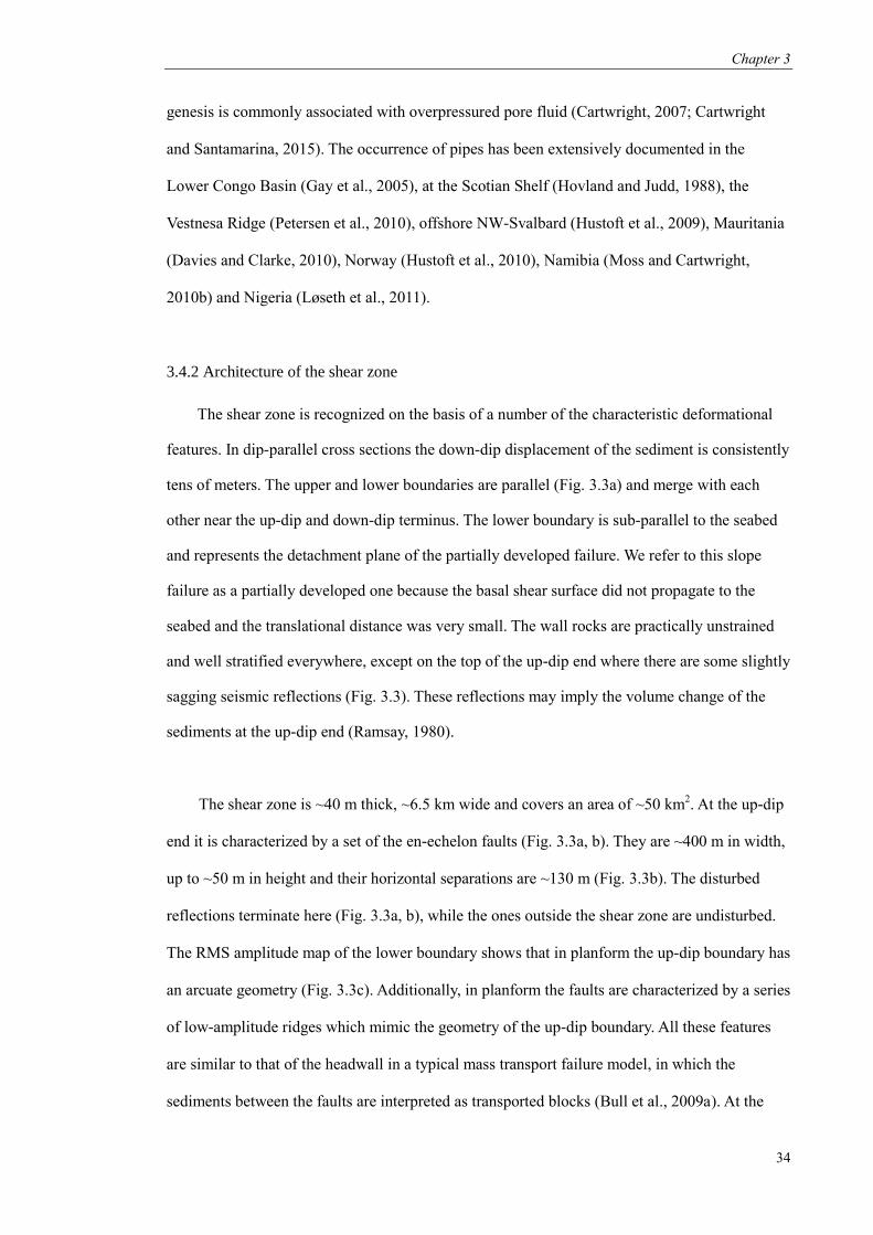
Chapter 3
34
genesis is commonly associated with overpressured pore fluid (Cartwright, 2007; Cartwright
and Santamarina, 2015). The occurrence of pipes has been extensively documented in the
Lower Congo Basin (Gay et al., 2005), at the Scotian Shelf (Hovland and Judd, 1988), the
Vestnesa Ridge (Petersen et al., 2010), offshore NW-Svalbard (Hustoft et al., 2009), Mauritania
(Davies and Clarke, 2010), Norway (Hustoft et al., 2010), Namibia (Moss and Cartwright,
2010b) and Nigeria (Løseth et al., 2011).
3.4.2 Architecture of the shear zone
The shear zone is recognized on the basis of a number of the characteristic deformational
features. In dip-parallel cross sections the down-dip displacement of the sediment is consistently
tens of meters. The upper and lower boundaries are parallel (Fig. 3.3a) and merge with each
other near the up-dip and down-dip terminus. The lower boundary is sub-parallel to the seabed
and represents the detachment plane of the partially developed failure. We refer to this slope
failure as a partially developed one because the basal shear surface did not propagate to the
seabed and the translational distance was very small. The wall rocks are practically unstrained
and well stratified everywhere, except on the top of the up-dip end where there are some slightly
sagging seismic reflections (Fig. 3.3). These reflections may imply the volume change of the
sediments at the up-dip end (Ramsay, 1980).
The shear zone is ~40 m thick, ~6.5 km wide and covers an area of ~50 km2. At the up-dip
end it is characterized by a set of the en-echelon faults (Fig. 3.3a, b). They are ~400 m in width,
up to ~50 m in height and their horizontal separations are ~130 m (Fig. 3.3b). The disturbed
reflections terminate here (Fig. 3.3a, b), while the ones outside the shear zone are undisturbed.
The RMS amplitude map of the lower boundary shows that in planform the up-dip boundary has
an arcuate geometry (Fig. 3.3c). Additionally, in planform the faults are characterized by a series
of low-amplitude ridges which mimic the geometry of the up-dip boundary. All these features
are similar to that of the headwall in a typical mass transport failure model, in which the
sediments between the faults are interpreted as transported blocks (Bull et al., 2009a). At the
Chapter 3
35
down-dip end we identify an imbricate fold and thrust system (Fig. 3.3d), which is a typical
feature in failures and this has been seen in offshore Israel (Martinez et al., 2005) and Norway
(Bull et al., 2009a). The thrust cannot be well detected but can be inferred empirically based on
the previous research (e.g. Lewis, 1971; Martinez et al., 2005). In planform the area covered by
the fold and thrust system is roughly 1200 m wide, 20 m high and the folds have an angle of dip
of 5°-6°. It is characterized by a series of convex-downslope ridges, buttressed against the
surrounding strata (Fig. 3.3e).
The lower boundary of the shear zone is a red-black (negative polarity) reflection (Fig.
3.4a). The strike-parallel seismic section shows that the upper boundary merges with the lower
one at the southeastern and northwestern margin of the shear zone, producing a wedge-like
geometry (Fig. 3.4a). In planform there is no clear difference between the amplitude values
inside and outside the shear zone (Fig. 3.4b). A series of high amplitude lineations can be seen
on the amplitude map of the lower boundary (Fig. 3.4c). The lineations can also be detected on
the dip-magnitude map and their terminations are aligned, thereby marking the side boundary of
the shear zone (Fig. 3.4d). Similar features have been seen in the Tampen Slide offshore
Norway (Solheim et al., 2005, Bull et al., 2009a).
3.4.3 High amplitude at the BSR
There are three high-amplitude zones revealed by an RMS amplitude map of the BSR in
the area of the shear zone (Fig. 3.5a – marked with HA1, HA2 and HA3). The area of HA1 is
lobe-shaped with its western end linking to the pipe cluster and partially connected to HA2 at
the eastern end of the lobe (Fig. 3.5). HA2 encompasses two high-amplitude features which
both have a width of ~400 m and a geometry of the band. Their orientation is SW-NE and sub-
parallel to the southern lateral margin of the shear zone (Fig. 3.5). The RMS amplitude value of
the BSR is highest at the central part of each band and declines gradually to both of its edges
(Fig. 3.5a). HA3 is in close proximity to the up-dip boundary and not completely within the
shear zone area (Fig. 3.5a). The portion within it, which is southwest of the up-dip boundary,
Chapter 3
36
displays a collection of linear features (Fig. 3.5a). The spacing between these features is
consistent with that of the low-amplitude ridges at the lower boundary (Fig. 3.3).
3.5 Interpretations
3.5.1 Hydrate-capped gas accumulation
Immediately below the BSR there are a series of the high amplitude reflections which have
negative polarities and form curvilinear bands in planform (Fig. 3.5b, c, d). This reflection
feature is consistent with the presence of gas accumulations at the level of the BSR, which
reduces the P-wave velocity and hence increases the acoustic impedance contrast (Andreassen et
al., 1997; Carcione and Tinivella, 2000; Haacke et al., 2007). This interpretation is in good
agreement with the typical configuration of gas accumulations underlying hydrate. It clogs the
pores of the host sediment and provides an effective baffle for underlying gases (Hornbach et
al., 2004; Tréhu et al., 2004; Bangs et al., 2005). Below the BSR the gas saturation calculated
from the well-log and seismic data could be 1-5% (Lu and McMechan, 2002), or as high as 17%
(Flemings et al., 2003) or even 90% (Tréhu et al., 2004). When the gas saturation is high
(>~10%), the capillary pressure in the gas-containing sediment may exceed the displacement
pressure of pore throats which is required to form a continuous filament of gas phase flow
(Schowalter, 1979). We interpret these bands to be narrow, elongate gas accumulations below
the hydrate. Even though most recorded values of gas saturation in the FGZ point towards a
continuous gas accumulation and it has been proposed before for this dataset as an explanation
for the development of seismic pipes (Davies et al., 2010), verifying that it was a connected gas
column is an uncertainty.
Near the southern part of the shear zone there are nine curvilinear high-amplitude bands
described by Davies et al. (2015; their fig. 2), two of which lie within the shear zone and
compose HA2. The bands appear to be sub-parallel to each other, similar in width and amplitude
variation. The geometry of the bands is a result of the intersection between the concave-up BSR
and the flat, less steep stratal reflection cross-cut by it (Fig. 3.6b, c, d). When the BSR cross-

Chapter 3
37
cuts the porous thin bed, it hosts hydrate above the BSR and gas below it, which will produce
high and low acoustic impedance, respectively. As a result, at the hydrate/gas contact a phase
reversal will show up on the seismic section (Fig. 3.6b, d). In HA3 some sub-vertical faults with
small offset (<10m) that occur near the up-dip boundary (Fig. 3.5d). The juxtaposed high
amplitude at the sides of the fault may imply the gas migration along the permeable faults.
3.5.2 Paleo-gas accumulation prior to the failure
The buoyancy effect of the interconnected gas accumulation can reduce the effective stress
of the sediment (Flemings et al., 2003). In this case the sediments that have the lowest effective
stress will be at the up dip, shallowest region of the gas accumulation. In the following section
we will semi-quantitatively assess the role of the buoyancy in priming the failure plane. To do
this we firstly estimate the extent of the paleo-gas accumulation prior to the failure. Even
though three independent gas accumulations (HA1, 2 and 3) are interpreted to be trapped below
the hydrate, the original geometry of the pre-failure gas accumulation may be different from
what it is now. A series of dip-parallel seismic sections (an example is shown in Fig. 3.7a) reveal
a potentially contiguous gas accumulation below the hydrate, although this is questioned after
we observe the planform amplitude map which shows this possible paleo-accumulation is
disrupted by a low-amplitude zone (Fig. 3.7b). We interpret that it did not exist until the failure
happened. A portion of gas located up-dip would migrate due to the fault activation and as a
result the remnant is HA3 (Fig. 3.5a). Nevertheless, the failure itself did not result in the
complete leakage of the underlying gas accumulation. After the failure partially developed, most
of the gas was still trapped below it. Therefore, it is very likely that these high-amplitude zones
are the remnants of a spatially more extensive pre-failure gas accumulation. This pattern of fluid
flow has been documented in the Eivissa Channel of the Western Mediterranean Sea, where the
overpressured pore fluids play a role in the repeated destabilization of the slope sediments
(Berndt et al., 2012).
Chapter 3
38
3.6 Discussion
3.6.1 Buoyancy and its effect
The buoyancy effect of the interpreted paleo-gas accumulation is equivalent to that of the
gas column marked in figure 7a. Its top and bottom correspond to the shallowest and deepest
point of the dipping pre-failure gas accumulation respectively. We estimate the height of the gas
column by using the TWTT data recorded in the seismic data and assuming the seismic velocity
in the seawater and the succession to be 1500 m/s and 1800 m/s respectively. This 263 m-high
gas column can produce considerable buoyancy pressure calculated by the liquid pressure
formula:
𝑃 = ∫ (𝜌𝑤 − 𝜌𝑔(𝑑)) 𝑔ℎ
0
𝑑𝑧
where 𝜌𝑔(𝑑) is the density of free gas (assumed to be 100% of methane, it varies with the depth
and could be calculated from the Clapeyron Equation), 𝜌𝑤 is the seawater density (1.024×10³
kg/m3), 𝑔 is the gravitational acceleration (9.81 m/s
2) and ℎ is the height of the gas column. At
the accumulation top, the pore pressure boosted by buoyancy would be sufficiently close to the
lithostatic pressure, which facilitated the forthcoming failure. The effective stress of the
sediment overlying the gas column, 𝜎′, has been significantly reduced (Fig. 3.7c). The shear
strength can be found in (Mello and Pratson, 1999; Jeager et al., 2008):
𝜎′𝑛𝑡𝑎𝑛𝜑 + 𝐶
where 𝜎′𝑛 is the effective normal stress, 𝜑 is the angle of the internal friction (30°, Nixon and
Grozic, 2006; Jeager J.C. et al., 2008) and 𝐶 is the cohesive strength (assumed to be zero,
Honbach et al, 2004; Nixon and Grozic, 2006). To compare the numeric relationship between
shear stress and shear strength under the guidance of Coulomb failure criterion (Jaeger and
Cook, 2007), we assume the gravity of overlying sediments as the only provider for the shear
stress:
𝜏 = 𝜌𝑠𝑔ℎ𝑠𝑠𝑖𝑛𝜃𝑐𝑜𝑠𝜃
where 𝜏 is the shear stress, 𝜌𝑠 is the sediment bulk density (assumed to be constant, 2.1×10³
kg/m3), ℎ𝑠 is the thickness of sediments above the BSR, 𝜃 is the angle of the continental slope

Chapter 3
39
(3°). The final result reveals that the shear stress exceeds the shear strength (0.27 MPa > 0.11
MPa), confirming the hypothesis that paleo gas accumulation is the potential primer for the
failure. In addition, the inverse calculation suggests that the critical height of gas column
required to fully prime the failure is 231 m (here we define that full priming happens when the
shear stress exceeds the sediment strength). Therefore, the sediments over the top 32 m high of
the paleo gas accumulation are fully primed (Fig. 3.8).
The semi-quantitative estimate of the buoyancy effect is entirely based on the 3-D seismic
dataset, which will unavoidably give rise to some uncertainties. Although we make reasonable
arguments that three high-amplitude zones once constituted an extensive gas accumulation prior
to the failure event, its precise geometry or extent is hard to determine. The lateral migration
along the base of the hydrate and changes in the position of the base of the HSZ would have led
to changes in the spatial extent of the gas accumulation once the gas started to accumulate
(Davies and Clarke, 2010). Furthermore, the inferred top and bottom ends of the gas column are
ambiguous as they are marked by the high amplitude fading instead of sudden termination. The
gradual variation of the amplitude values makes the interpretive decision of the gas
accumulation margin less accurate. Therefore, determining the precise height of the gas column
prior to the failure seems impossible in this case.
3.6.2 Preserved overpressure
When the base of the HSZ resets upwards, the released methane progressively adds to the
gas column until the excess pore pressure can be cumulated until the shear surface is critically
stressed. Such process of the overpressure build-up could be disturbed by the seismic pipes
because they are good conduits with pressure communication. They are probably clusters of
fractures and will discharge overpressured pore fluids to zones of lower pressure (Hovland and
Judd, 1988; Cartwright, 2007; Hustoft et al, 2007; Liu and Flemings, 2007; Cartwright and
Santamarina, 2015). Thus it is reasonable to speculate when pipes passing through the gas
accumulation, they would have hindered the development of overpressure (Davies et al., 2010).
Chapter 3
40
Only 8 seismic pipes occur within the failure area and, more importantly, all these pipes
terminate below or at the BSR (Fig. 3.2e). This supports the notion that excess pore pressure
could have developed at the level of the BSR in the area of the failure. In contrast, outside the
failure we identify 22 seismic pipes (diameter > 100 m). In particular, 5 of these pipes pass
through the base of the hydrate marked by the BSR with their tops occurring immediately below
the seafloor. The presence of these pipes implies the seal by-passing at the level of the BSR
(Cartwright, 2007; Moss and Cartwright, 2010b). In summary, the distribution of pipes and their
spatial relationship with the BSR may indicate the possible locations where high pore pressure
could have developed.
3.6.3 Dissociation-related failure mechanism
Hydrate dissociation is commonly considered as a trigger for submarine slope failure and
there are models proposed for the Storegga Slide (Sultan et al., 2004) and the Blake Ridge
(Dillon et al., 2001). In general, the key of this mechanism is a decomposed zone where
hydrates were trapped before but later dissociated due to the sedimentation or the variation of
the bottom water temperature (McIver, 1982, their fig. 4). The huge volumetric expansion
during the dissociation of these hydrates can lower the effective stress and thus reduce the
strength of sediment in the decomposed hydrate layer. Additionally, once dissociation has
occurred the hydrates no longer play a role in the cementation and consolidation of the host
sediment (Xu and Germanovich, 2006), which further reduces the effective stress and facilitates
the imminent failure. According to the failure model associated with hydrate dissociation, the
most likely position for the failure plane would be near the base of the decomposed zone due to
its relatively high concentration of gas hydrate (McIver, 1982). We cannot be completely sure
that hydrate dissociation had no role in priming this partially developed submarine landslide.
But there is no evidence to support this.

Chapter 3
41
3.7 Conclusions
We propose this is a rare example where the evidence for the failure mechanism is
preserved because slope failure did not go to completion. Although the evidence for a
contiguous gas column at the time of failure is not conclusive, buoyancy-related mechanism for
submarine failure is more likely than hydrate dissociation. Our preferred model is that this
process starts with a paleo gas accumulation below the hydrate and as more gases accumulated,
the vertical height of the gas accumulation increased until the pore pressure reached a level such
that shear strength of bedding planes was achieved and the feature was then susceptible to an
external trigger. This model highlights the role of the gas accumulation trapped by the hydrate in
the formation of submarine failures.
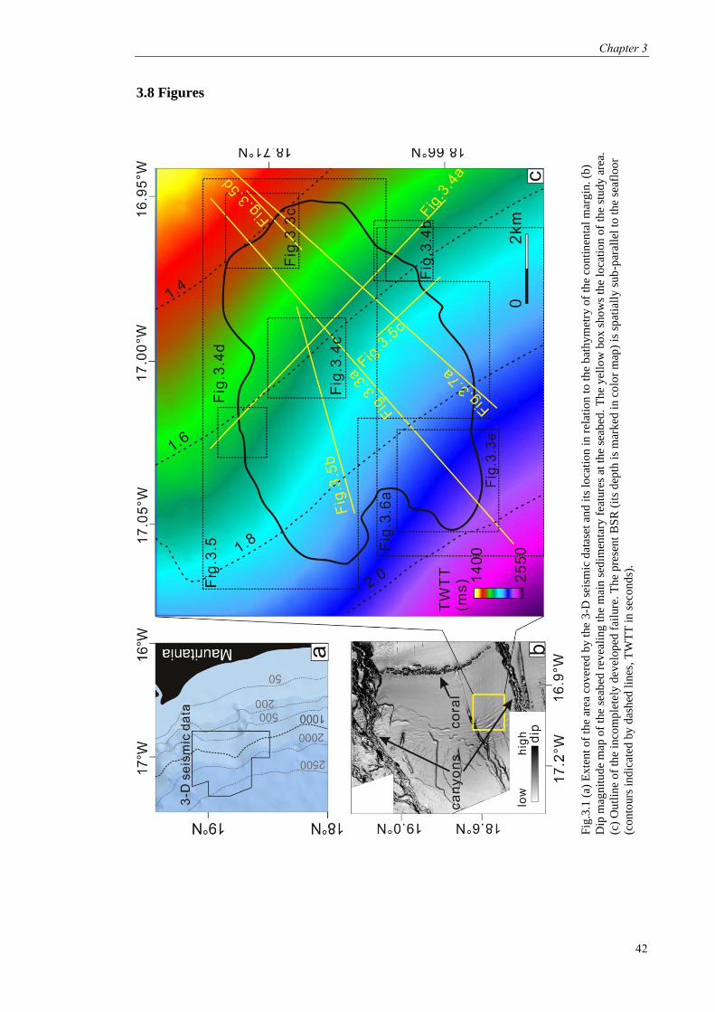
Chapter 3
42
3.8 Figures
Fig
.3.1
(a)
Ex
ten
t o
f th
e ar
ea c
ov
ered
by
th
e 3
-D s
eism
ic d
atas
et a
nd
its
lo
cati
on
in
rel
atio
n t
o t
he
bat
hy
met
ry o
f th
e co
nti
nen
tal
mar
gin
. (b
)
Dip
mag
nit
ud
e m
ap o
f th
e se
abed
rev
eali
ng
th
e m
ain
sed
imen
tary
fea
ture
s at
th
e se
abed
. T
he
yel
low
bo
x s
ho
ws
the
loca
tio
n o
f th
e st
ud
y a
rea.
(c)
Ou
tlin
e o
f th
e in
com
ple
tely
dev
elop
ed f
ailu
re.
Th
e p
rese
nt
BS
R (
its
dep
th i
s m
ark
ed i
n c
olo
r m
ap)
is s
pat
iall
y s
ub
-par
alle
l to
th
e se
aflo
or
(co
nto
urs
in
dic
ated
by
das
hed
lin
es,
TW
TT
in
sec
on
ds)
.

Chapter 3
43
Fig
.3.2
(a-
d)
Sei
smic
fea
ture
s o
f ty
pic
al p
ipes
. T
he
ori
enta
tio
ns
of
thes
e se
ism
ic c
ross
sec
tio
ns
are
no
t sh
ow
n h
ere.
(e)
Dip
mag
nit
ud
e m
ap o
f B
SR
, sh
ow
ing
th
e lo
cati
on
of
pip
es t
erm
inat
ing
at
or
bel
ow
th
e B
SR
(m
ark
ed i
n y
ello
w c
ircl
e) a
nd
by
pas
sin
g t
he h
ydra
te-c
on
tain
ing
sed
imen
t (m
arked
in
red
cir
cle)
. N
ote
th
at n
o p
ipes
pen
etra
te
the
BS
R i
n t
he
area
of
the
shea
r zo
ne.
Th
e d
ash
ed w
hit
e li
ne
mar
ked
th
e ar
ea o
f th
e sh
ear
zon
e.
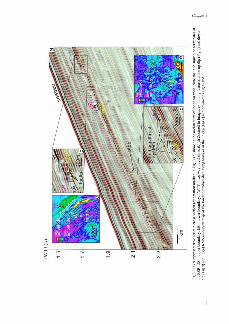
Chapter 3
44
Fig
.3.3
(a)
A r
epre
sen
tati
ve
seis
mic
cro
ss s
ecti
on
(o
rien
tati
on
mar
ked
in
Fig
. 3
.1c)
sh
ow
ing
th
e ar
chit
ectu
re o
f th
e sh
ear
zon
e. N
ote
th
at a
sei
smic
pip
e te
rmin
ates
at
the
BS
R.
UB
– u
pp
er b
oun
dar
y,
LB
– l
ow
er b
oun
dar
y,
TW
TT
– t
wo
way
tra
vel
tim
e. (
b)(
d)
Zo
om
ed-i
n i
mag
es e
xh
ibit
ing
fea
ture
s at
th
e u
p-d
ip (
Fig
.b)
and
do
wn
-
dip
(F
ig.d
) en
d. (c
)(e)
RM
S a
mp
litu
de
map
of
the
low
er b
ou
nd
ary
dis
pla
yin
g f
eatu
res
at t
he
up
-dip
(F
ig.c
) an
d d
ow
n-d
ip (
Fig
.e)
end
.

Chapter 3
45
Fig
.3.4
(a)
A r
epre
sen
tati
ve
seis
mic
lin
e (o
rien
tati
on
mar
ked
in
Fig
.3.1
c) s
ho
win
g t
he
arch
itec
ture
of
the
shea
r zo
ne.
(b)(
c) R
MS
am
pli
tud
e m
ap o
f th
e lo
wer
bo
und
ary
ex
hib
itin
g i
ts p
lan
form
fea
ture
s. (
d)
Dip
mag
nit
ude
map
of
the
low
er b
oun
dar
y.
No
te t
he
rid
ges
occ
ur
bo
th o
n t
he
amp
litu
de
map
and
dip
-
mag
nit
ud
e m
ap.

Chapter 3
46
Fig
.3.5
(a)
RM
S a
mp
litu
de
map
of
the
pre
sen
t B
SR
, sh
ow
ing
th
ree
area
s w
ith
hig
h s
eism
ic a
mp
litu
de
(nam
ed H
A1
, H
A2 a
nd
HA
3).
Th
e w
este
rn e
nd
of
HA
1 i
s
stra
tig
rap
hic
ally
lin
ked
to
th
e to
p o
f p
ipe
clu
ster
s. P
art
of
HA
3 s
tay
s o
uts
ide
the
shea
r zo
ne
and
is
inte
rpre
ted a
s g
as l
eak
age.
SZ
– s
hea
r zo
ne.
(b
-d)
Sei
smic
sect
ion
s d
isp
lay
ing
hig
h a
mp
litu
de
refl
ecti
on
s w
ith
in t
hre
e h
igh
-am
pli
tud
e ar
eas.
Th
e ‘b
and’
is a
sei
smic
fea
ture
of
the
BS
R,
des
crib
ing
its
geo
met
ry o
f h
igh
-
amp
litu
de
sect
ion
in
pla
nfo
rm. It
is
furt
her
dis
cuss
ed i
n s
ecti
on
5.
PR
– p
has
e re
ver
sal.

Chapter 3
47
Fig
.3.6
(a)
RM
S a
mp
litu
de
map
of
BS
R s
ho
win
g a
ser
ies
of
hig
h a
mp
litu
de
ban
ds
surr
ou
nd
ing
th
e so
uth
ern m
arg
in o
f th
e sh
ear
zon
e. (
b)
Sch
emat
ic m
od
el o
f h
ow
hig
h a
mp
litu
de
ban
d f
orm
ed. R
efle
ctio
n X
rep
rese
nts
a p
oro
us
bed
cro
ss-c
ut
by
th
e B
SR
. A
I –
aco
ust
ic i
mp
edan
ce.
FG
Z –
fre
e g
as z
on
e. (
c) S
eism
ic s
ecti
on
sho
win
g t
he
rela
tion
ship
bet
wee
n B
SR
an
d b
and
s. W
her
e st
rata
is
cro
ss-c
ut
by
th
e B
SR
is
com
mo
nly
mar
ked
by
sei
smic
ph
ase
rev
ersa
l. H
A –
hig
h a
mp
litu
de,
PR
– p
has
e re
ver
sal.
(d
) L
ine
dra
win
g o
f fi
gu
re c
. T
he
ph
ase
rev
ersa
l is
th
e re
sult
of
the
thin
po
rou
s b
eds
con
tain
ing
hy
dra
tes
abo
ve
the
BS
R a
nd
gas
es b
elo
w i
t.
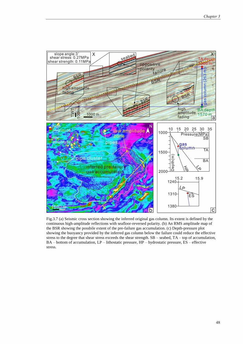
Chapter 3
48
Fig.3.7 (a) Seismic cross section showing the inferred original gas column. Its extent is defined by the
continuous high-amplitude reflections with seafloor-reversed polarity. (b) An RMS amplitude map of
the BSR showing the possbile extent of the pre-failure gas accumulation. (c) Depth-pressure plot
showing the buoyancy provided by the inferred gas column below the failure could reduce the effective
stress to the degree that shear stress exceeds the shear strength. SB – seabed, TA – top of accumulation,
BA – bottom of accumulation, LP – lithostatic pressure, HP – hydrostatic pressure, ES – effective
stress.

Chapter 3
49
Fig
.3.8
Th
e sc
hem
atic
dia
gra
m o
f th
e b
uoy
ancy
-rel
ated
fai
lure
mec
han
ism
. T
he
gas
acc
um
ula
tes
un
der
th
e h
yd
rate
(m
ark
ed b
y t
he
BS
R)
and
form
s a
26
3 m
-hig
h g
as c
olu
mn
. It
pri
mes
th
e o
ver
lyin
g s
edim
ent
ho
stin
g h
ydra
te,
wh
ere
no
pip
es d
evel
op
. T
he
crit
ical
hei
gh
t o
f th
e g
as
colu
mn
is
~2
31
m.
Wh
en t
he
shea
r st
ress
is
less
th
an t
he
shea
r st
ren
gth
, th
e fa
ilu
re p
lan
e is
un
der
-pri
med
. H
P –
hy
dro
stat
ic p
ress
ure
, L
P –
lith
ost
atic
pre
ssu
re,
TA
– t
op
of
accu
mu
lati
on
, B
A –
bo
tto
m o
f ac
cum
ula
tio
n,
GA
– g
as a
ccu
mu
lati
on
, R
T –
ro
of
thru
st,
FT
– f
loo
r th
rust
.

Chapter 4
50
Chapter 4 Methane Hydrate Recycling probably after the Last Glacial Maximum
Ang Li a*
, Richard J. Davies b, Simon Mathias
a
a Centre for Research into Earth Energy Systems (CeREES), Department of Earth Sciences,
Science Labs, Durham University, DH1 3LE, UK b School of Civil Engineering and Geosciences, Newcastle University, Newcastle upon Tyne,
Tyne and Wear, NE1 7RU, UK
Abstract:
To what extent methane liberated from marine hydrate will enter the ocean during a warmer
world is unknown. Although methane release due to hydrate dissociation has been modelled, it
is unclear whether or not methane will reach the seafloor during a warmer world and therefore
contribute to oceanic and atmospheric budgets. Here we show, using a new three-dimensional
(3-D) seismic dataset, that some hydrate deposits surround the gas chimneys passing through
the HSZ. Bottom water warming since the last glacial maximum (LGM) is speculated to cause
hydrate dissociation but critically some of the released methane was not vented to the ocean.
The released gas caused seal failure and free gas entered the hydrate stability zone (HSZ)
through vertical gas chimneys to where new hydrate accumulations formed. This process is a
new evidence for methane recycling and could account in part for the lack of methane in ice
core records that cover warming events during the late Quaternary. This research provides new
insight into how methane could be recycled rather than vented during a warmer world.
Key words: gas hydrate, gas chimney, BSR, methane recycling

Chapter 4
51
4.1 Introduction
Methane is a potent greenhouse gas and vast quantities of it are locked in marine hydrate
along the continental margins (Kvenvolden, 1993). Methane released from hydrate could have a
role in accelerated climatic warming, ocean acidification and de-oxygenation (Biastoch et al.,
2011; Dickens, 2003). There is already potential evidence, such as plumes of gas bubbles, for
methane liberated from hydrates venting into the ocean due to oceanic warming in the Arctic
(Westbrook et al., 2009) and along the US Atlantic margin (Phrampus and Hornbach, 2012;
Skarke et al., 2014). But isotopic records that cover rapid Quaternary climate change events
from ice cores of polar region indicate that methane from hydrate is not released during periods
of rapid warming (Sowers, 2006). Methane stored in hydrate is probably a contributor rather
than the main source of atmospheric methane budget after the last glacial maximum (LGM,
Chappellaz et al., 1993). The fundamental question of whether large amount of methane from
hydrate escapes into oceans and the atmosphere remains unanswered. If it did not reach the
seabed, how is methane retained in the subsurface?
Hydrates are usually identified in marine settings through the identification of bottom
simulating reflectors (BSRs) in seismic reflection datasets. BSRs mark the base of the hydrate
stability zone (BHSZ) below which free gas is often trapped and this configuration yields a
medium to high acoustic impedance contrast (Shipley et al., 1979). As the water depth shallows
at continental margins, the BSR also shoals and seismic imaging sometimes shows examples of
it intersecting the seabed at a water depth between ~350 and ~600 m (Boswell and Collett,
2011). In general the ascent of methane into the hydrate stability zone (HSZ) should be impeded,
as hydrates clogs interconnected pores and fractures (Nimblett and Ruppel, 2003). But methane
can sometimes pass through the HSZ and arrive at the seabed (Liu and Flemings, 2006).
Seismic evidence for this methane venting is often gas chimneys with pockmark at the seabed
and they are thought to represent the occurrence of vertical migration of pore fluid (Hovland
and Judd, 1988; Cartwright and Santamarina, 2015).

Chapter 4
52
Venting into the atmosphere is not necessarily the fate of gas that has been liberated from
methane hydrate. Methane could be recycled to the BHSZ (Davies and Clarke, 2010; Paull et al.,
1994), dissolved into the ocean and replaced by other gases such as oxygen during its ascent
(McGinnis et al., 2006) and oxidised aerobically in the shallow ocean (Ward et al., 1987) or
anaerobically in the sub-seabed sediment (Hoehler et al., 2000). Using a new 3-D seismic
survey offshore of Mauritania, we consider the fate of methane liberated due to oceanic
warming since the LGM as a potential scenario for how marine hydrates will behave due to a
future warmer world.
4.2 Geological setting
The area covered by the 3-D seismic survey is offshore of Mauritania (Fig. 4.1) where the
water depth ranges from 50 to 1800 m (Fig. 4.1b). The shelf-slope break occurs at ~120 m water
depth and the continental slope dips at ~3°. In the southeast of the survey there are a number of
canyons that are part of the Cap Timiris Canyon system. The study area is located between two
of these canyons and covers an area of ~23 km2 and the uppermost ~100 m of the sedimentary
succession. It is most likely dominated by the fine-grained hemi-pelagic sediment interbedded
with turbidite mud and sand, deposited during alternating climatic periods of aridity and
humidity in the Pleistocene and Holocene (Henrich et al., 2008; Zühlsdorff et al., 2007). The
gravity cores of GeoB 8507-3 (Fig. 4.1a) record the uppermost 10 m-thick sediments in the
Timiris Canyon and show that the sedimentation rate averages at 190 m/my (metres per million
years) in the Holocene (Zühlsdorff et al., 2007), but this rate may not be typical in the study area.
This rate can be up to 685 m/my in the records of GeoB 8509-2 (Zühlsdorff et al., 2007). The
commercial wells, Ras Al Baida-1 and Al Kinz-1, show that there are traces of hydrocarbons
throughout late Cretaceous and Paleogene sediments (Vear, 2005).

Chapter 4
53
4.3 Seismic data and methodology
The 3-D seismic data cover an area of ~3800 km2. The bin spacing is 12.5 m × 25 m. The
recording is cut by a frequency filter of 3 – 200 Hz. The dominant frequency in the upper 100
m-thick sediment is 55 Hz. These data have a sampling rate of 2 ms and are zero-phased. They
are displayed in the depth domain after being Kirchoff depth migrated. The velocity model for
this migration is not provided in this research. A positive polarity is defined by a peak on the
seismic trace and displayed by a black-red-black seismic loop on the cross section, which
represents an increase in the acoustic impedance. The extracted seismic attributes include RMS
(root mean square) amplitude and dip-magnitude. The maps of these attributes are utilised to
pinpoint the hydrate/gas and visualise the migration-related features (e.g. pockmarks) in an area
of interest.
The BSR is picked along the troughs of the seismic traces that together produce a reflection
usually cross-cutting the stratal reflections. At the places where this cross-cutting cannot be
identified the BSR depth is inferred by linear interpolation or consistent with the high-amplitude,
horizon-parallel reflection. A numerical model for 2-D heat conduction is used to simulate the
location of the BHSZ (appendix 2) and validate the interpretation of the BSR.
4.4 Observations
4.4.1 Seabed and BSR
The seabed dips to the southwest and only one pockmark (~200 m in diameter) is found to
the northeast of the landward terminus of the BSR (Fig. 4.1b). No seabed amplitude anomaly
can be seen in or near this pockmark, indicating the absence of the carbonate crust that has been
documented at venting sites (e.g. Hovland et al., 1987). The BSR is observable over most of the
region at the water depths of 750 – 1300 m, dipping at ~4° and deepening southwestern. On a
seismic profile it is characterised by a negative high-amplitude reflection and cross-cutting
stratal reflections at low angles (<5°) (Fig. 4.2). The BSR does not intersect with the seabed
reflection. Instead, it often terminates at ~70 mbsf (metres below the seafloor) (Fig. 4.2a). The

Chapter 4
54
seabed intersection depth (SID) is estimated by the numerical model of heat conduction to be
711 m (Fig. A2.1, appendix 2), though at some sites outside the study area we observe that the
SID is ~740 m.
4.4.2 Seismic chimneys and high-amplitude anomalies
4.4.2.1 Seismic chimneys
15 seismic chimneys have been identified in the study area. They are 130 – 180 m in
height, 80 – 200 m in diameter and characterised by vertically aligned discontinuities in seismic
reflections (Fig. 4.3). The discontinuity takes the form of a localised, sub-circular region of
positive relief at each reflection above the BSR. The relief is 5 – 10 m and the diameter of the
regions of positive relief maximises at the reflections D and E (Fig. 4.4). Apart from the
reflections near to the top of the gas chimney (e.g. reflection B, Fig. 4.3, 4.4), those inside the
chimneys have lower amplitude than surrounding reflections. The observations are similar to
gas chimneys identified offshore mid-Norway (Hustoft et al, 2010). The bases of the gas
chimneys are identified on the basis of where reflections show no deflection. We also see that
the alignment of the bases is sub-parallel to the present BSR. The root zone is 30 – 70 m below
the present BSR (Fig. 4.3). Their tops are located at the reflection immediately below the seabed
but there is no evidence, such as pockmarks, for their presence at the current seabed (Fig. 4.3).
The chimneys are most unlikely to be the velocity pull-up artefacts. Such artefacts are
characterised by distorted reflections or obscure imaging vertically below the anomalous
velocity unit, while in this case the reflections in the deep subsurface are intact and show no
difference with the nearby reflections (Fig. 4.3).
4.4.2.2 High-amplitude anomalies
Around the seismic chimneys, but only detected by mapping certain reflections (D and E,
Fig. 4.3c) are sub-circular, sub-elliptical or irregularly shaped high amplitude anomalies that
have the same polarity with the seabed (Fig. 4.3 and 4.4). We term these ‘positive high-
amplitude anomalies’ (PHAAs). They are ~70 m below the seabed and ~2.4 km away from the

Chapter 4
55
termination of the BSR in the seaward direction. Chimney 10 for example, is surrounded by
three regions of high amplitude, each with an irregular geometry. The high-amplitude values
among these regions occur closest to the chimney (Fig. 4.4). The isolated PHAA adjacent to
chimney 7 covers an area of ~0.08 km2 and has a sub-elliptical geometry. Its long axis is sub-
parallel to the dip of the continental slope. The amplitude values of this PHAA are largest near
the gas chimney and diminish progressively along the reflections towards its periphery. In plan-
view, chimney 7 is not in the centre of the PHAA. A third example has two associated chimneys
(8 and 12, Fig. 4.4). They both are surrounded by PHAAs which coalesce to form a larger
PHAA with an area of 0.21 km2. Again in plan form these two chimneys are not central to their
respective PHAAs (Fig. 4.4).
4.5 Interpretation
4.5.1 Gas trapped below the BSR
The amplitude map of the BSR shows a set of high-amplitude bands (Fig. 4.2).
Similar bands have been identified before offshore of Mauritania (Li et al. 2016). In both
examples they have the opposite polarity to the seabed (Fig. 4.2a), suggesting a decrease in
acoustic impedance. There are also multiple phase reversals along the BSR (Fig. 4.2a, c). They
occur at the edge of the band, where we predict the pores of the thin beds are filled with hydrate
above the BSR and gas below it, producing high and low acoustic impedance, respectively (Fig.
4.2c). The transition of the seismic phase in a step-like pattern in space causes the aligned high-
amplitude termination along the BSR. This configuration coincides with the other known
marine hydrate systems (e.g. Bünz and Mienert, 2004).
Representative seismic lines where these enhanced reflections are present show that the gas
chimneys root into a zone below the BSR (marked FGZ on Fig. 4.3). This spatial relationship,
coupled with the knowledge that the gas chimneys are probably a migration pathway for pore
fluid (Cartwright and Santamarina, 2015) implies that free gas trapped below the BSR was

Chapter 4
56
transported to the shallower subsurface. Because there is no evidence for pockmarks or indeed
any other morphological features at the seabed we propose there was no significant escape of
methane into the ocean. Therefore, similar to Ivanov et al. (2007), the gas chimneys did not
intersect a free surface.
4.5.2 Hydrate deposits
The PHAAs are interpreted to be primarily caused by gas hydrate deposits that have a
higher P-wave velocity, probably between 3760 – 4000 m/s (Sloan and Koh, 2008), than that of
the pore fluid of seawater filling in background sediment. A high hydrate saturation (e.g. >35%,
Hornbach et al., 2003) can increase the acoustic impedance of hydrate-filled sediment to the
level such that should be detected on seismic dataset. The thickness of the PHAAs is estimated
to be up to ~16 m at the seismic scale based on the vertical resolution of ~8 m (the P-wave
velocity of the seawater-filled sediment is assumed to be 1800 m/s and the vertical resolution is
one quarter of the wavelength). But gravity cores sampled at the Timiris Canyon indicate the
thickness of sands is likely to be no more than 10 m (Zühlsdorff et al., 2007). Therefore, we
think the PHAA is the seismic response to one or more than one hydrate-containing porous
sands.
We propose the hydrate accumulations were sourced from free gas transported through the
gas chimneys. Methane carried within pore fluid migrated through the fractures and then flowed
laterally along permeable beds in an up dip direction where hydrate would have formed around
the chimney point source (Davies et al., 2014; Xu and Ruppel, 1999). As the PHAAs are
discrete regions surrounded by lower seismic amplitudes, our preferred interpretation is that
hydrate at this level was absent or at a low concentration before the chimneys formed and fed
the new hydrate accumulations.
Our interpretation suggests that the geometry of the PHAA is the result of methane
migration after leaving the gas chimneys. Given that the pore fluid could form a frictionless
Chapter 4
57
buoyant gravity current, its spreading out will be a function of the time, the density difference,
the input flux and the effective permeability of the porous medium (Lyle et al., 2005). As the
base of the dipping cap rock can be considered as an inclined plane and there is a density
contrast between free gas and seawater, the buoyancy has a role in driving the fluid migrating
up dip, which leads to the ellipsoidal geometry of the PHAA elongated in the direction that is
parallel to the dip of the continental margin (Vella and Huppert, 2006). Such a pattern of
migration has been seen in the Sleipner field of the North Sea, where CO2 has been injected into
subsurface sands. The geometry of the CO2 reservoir can be detected by the seismic imaging
that displays a comparable high amplitude zone (Boait et al., 2012). Another example of this
geometry is lateral migration of gas along the BHSZ offshore of Mauritania, in which case tear-
drop shaped high amplitudes that loop around and envelope point-source gas chimney have
been imaged (Davies et al., 2014).
It cannot be completely ruled out that the PHAAs are the seismic response to the
authigenic carbonate-cemented sediment. An example outcropping at the seabed was seen in the
Gulf of Mexico (Roberts et al., 2006). The carbonate cements could form as a result of
anaerobic methane oxidation that develops in the methane-rich environment (Hovland et al.,
1987). But the PHAAs, which are ~70 mbsf, may be too deep for this methane oxidation to take
place as the sulfate-methane interface (SMI), which is at the base of the sulfate reduction zone,
is normally at < 70 mbsf (Borowski et al., 1999).
4.6 Discussion
4.6.1 Methane passing through the HSZ
In general methane entering the HSZ will be trapped within it in some way or added to its
base when the base of HSZ deepens, but free gas can also exist within or pass through the HSZ.
Some hypotheses have been proposed to explain this phenomenon. (a) Once gas enters the HSZ,
it will form hydrates, depleting pore water and therefore increasing its salinity (Liu and

Chapter 4
58
Flemings, 2006). Furthermore, the hydrate clogging slows the removal of the highly
concentrated ionised salt (Milkov et al., 2004). The resulting hypersaline pore environment will
inhibit further hydration (Sloan and Koh, 2008) and this will allow gas for some time to pass by
(Liu and Flemings, 2006; Liu and Flemings, 2007). (b) Excessive methane may consume all in-
situ water to form hydrate, which will create a water-free environment in the low-permeability
sediment without no more gas being trapped (Tréhu et al., 2004). In this case all the water can
be depleted when the methane accounts for >70.8% of the total volume of pore fluid (the in-situ
temperature and pressure are 10.23 oC and 9.54 MPa respectively). (c) Where the chimney
intersects with the BSR, the base of the HSZ is redefined by the vertical intrusion of the warm
advecting fluid. The perturbation zone, which coincides with the outline of gas chimney, is
physically stable for gas to exist (Wood et al., 2002). Here either one or any combination of
these mechanisms may contribute to the process of gas passing through the HSZ.
4.6.2 Model
We interpret that the gas chimneys did not reach the modern seabed. The vertical distance
between the tops of the gas chimneys and the seabed reflection cannot be clearly identified in
the seismic dataset and is probably less than 8 m (vertical resolution). Given that the
sedimentation rate ranges from 190 m/my to 685 m/my (Zühlsdorff et al., 2007), the age of the
gas chimneys is estimated to be up to 12 – 42 kyr. A prominent, millennial-scale warming event
in the past 12 – 42 kyr is the global warming since the LGM that is interpreted to cause the
upward shift of the BHSZ and hence the hydrate re-incorporation. The interpretation of this shift
is consistent with those in offshore of Oregon (Bangs et al., 2005) and on the Cascadia margin
(Musgrave et al., 2006). We did not rule out the possibility that this warming event could be
older than the LGM due to the uncertainty of the sedimentation rate. To probe into how this
hydrate re-incorporation took place, we introduce the numerical modelling.
Here we developed a 2-D finite diffusive heat-flow model that allows us to propose how
the hydrate deposit formed after the LGM (Fig. 4.5, appendix). The model output of the

Chapter 4
59
variation of the bottom water temperature (BWT, Bintanja and van de Wal, 2008) and the
relative sea level (RSL, Siddall et al., 2003) are taken as the input into this model to predict the
shift of the BHSZ since the LGM. We determine the geothermal gradient by seeing whether the
modelled BHSZ at steady state has a good match with the seismic observation (35 oC km
-1,
appendix 2). The modelling results, which are impacted by the uncertainties of the input
parameters (appendix 2), show that the BHSZ probably has shoaled by ~60 m since the LGM.
The thinning of the HSZ caused dissociation of the hydrate located at the BHSZ. The buoyancy
of the released gas would have generated excess pore pressure that could have led to the
development of hydraulic fractures (Xu and Germanovich, 2006). Therefore, the gas chimneys
are interpreted to form during the period of rapid shallowing of the BHSZ. The hydrate started
to accrete after the gas conduit was established between the sediments below the BHSZ and at
the level of reflections D and E. Since then the hydrate accretion would continue as the BHSZ
shoaled (Fig. 4.5). It is unlikely but cannot be ruled out entirely that the spatial relationship
between the gas chimneys and the BSR is coincident.
4.6.3 Implications
The presence of the hydrate deposits implies that some of the gases released from hydrate
since the LGM were recycled. We propose the sediments above the base of the HSZ prevent the
escape of methane. The amount of methane recycled as hydrate can be amplified once this
process has repeated at multiple horizons (e.g. Davies et al., 2014). But the volume of these
accumulations is significantly lower than that of sediment that would have undergone
dissociation after the LGM, which implies there are other mechanisms related to trapping and
consuming methane. To our knowledge, they involve methane oxidisation (Treude and Ziebis,
2010), being trapped stratigraphically in situ, or recycled as new hydrate at the base (Davies and
Clarke, 2010; Paull et al., 1994). To what extent methane can be re-incorporated before reaching
seabed is still a question to be answered. But this mechanism is speculated to account in part for
why ice cores do not record methane from marine hydrate during episodes of rapid climatic
warming.

Chapter 4
60
4.7 Conclusions
We found a good example for the re-incorporation of methane into hydrate during oceanic
warming. Due to this warming methane released from hydrate entered the HSZ via vertical
fractures and was recycled as marine hydrate. From this model we can say methane escape
towards the seabed was buffered. This offers a new evidence for methane recycling that could in
part explain why methane from marine hydrates is not thought to be a main contributor to the
atmospheric budget.

Chapter 4
61
4.8 Figures
Fig
.4.1
(a)
Lo
cati
on o
f th
e 3
-D s
eism
ic s
urv
ey.
(b)
Bat
hy
met
ric
map
sh
ow
ing t
he
morp
holo
gy
of
the
seab
ed.
Red
box
– s
tud
y a
rea.
PM
– p
ock
mar
k. (c
)
Th
e R
MS
am
pli
tud
e m
ap o
f th
e B
SR
in
th
e st
ud
y a
rea.
Red
das
hed
lin
e m
ark
s th
e la
nd
war
d e
xte
nt
of
BS
R a
nd
bla
ck d
ashed
lin
es r
epre
sen
t is
ob
ath
s. T
he
seis
mic
fea
ture
s o
f b
and
s (B
) ar
e in
terp
rete
d i
n s
ecti
on
5.1
. C
– c
any
on,
HA
– h
igh
am
pli
tud
e, L
A –
lo
w a
mp
litu
de
in t
his
an
d s
ub
seq
uen
t fi
gu
res.

Chapter 4
62
Fig
.4.2
(a)
A r
epre
sen
tati
ve
seis
mic
sec
tio
n s
ho
win
g t
he
typ
ical
fea
ture
s o
f a
BS
R a
nd
th
e
gas
acc
um
ula
tio
ns
seal
ed b
enea
th
it.
B-r
-b a
nd r
-b-r
ref
er t
o t
he
bla
ck-r
ed-b
lack
an
d r
ed-b
lack
-red
seis
mic
lo
op
, re
spec
tiv
ely
. (b
) T
he
RM
S a
mp
litu
de
map
of
the
BS
R
dis
pla
yin
g t
hre
e st
rik
e-p
aral
lel
hig
h a
mp
litu
de
ban
ds
(mar
ked
by
I, I
I an
d I
II).
(c)
In
terp
reta
tion o
f
the
cro
ss s
ecti
on
X-X
’. A
t th
e
seaw
ard
ed
ge
of
the
ban
d f
eatu
re,
ph
ase
rev
ersa
l so
met
imes
can
be
seen
. T
he
gre
y c
olo
ur
rep
rese
nts
a
set
of
po
rou
s th
in b
eds
inte
rbed
ded
wit
h l
ess
po
rou
s o
nes
. T
he
bri
gh
ter
red
an
d y
ello
w c
olo
urs
mar
k t
he
hig
her
sat
ura
tion
of
hyd
rate
and
gas
, re
spec
tiv
ely
. P
R –
ph
ase
rev
ersa
l.
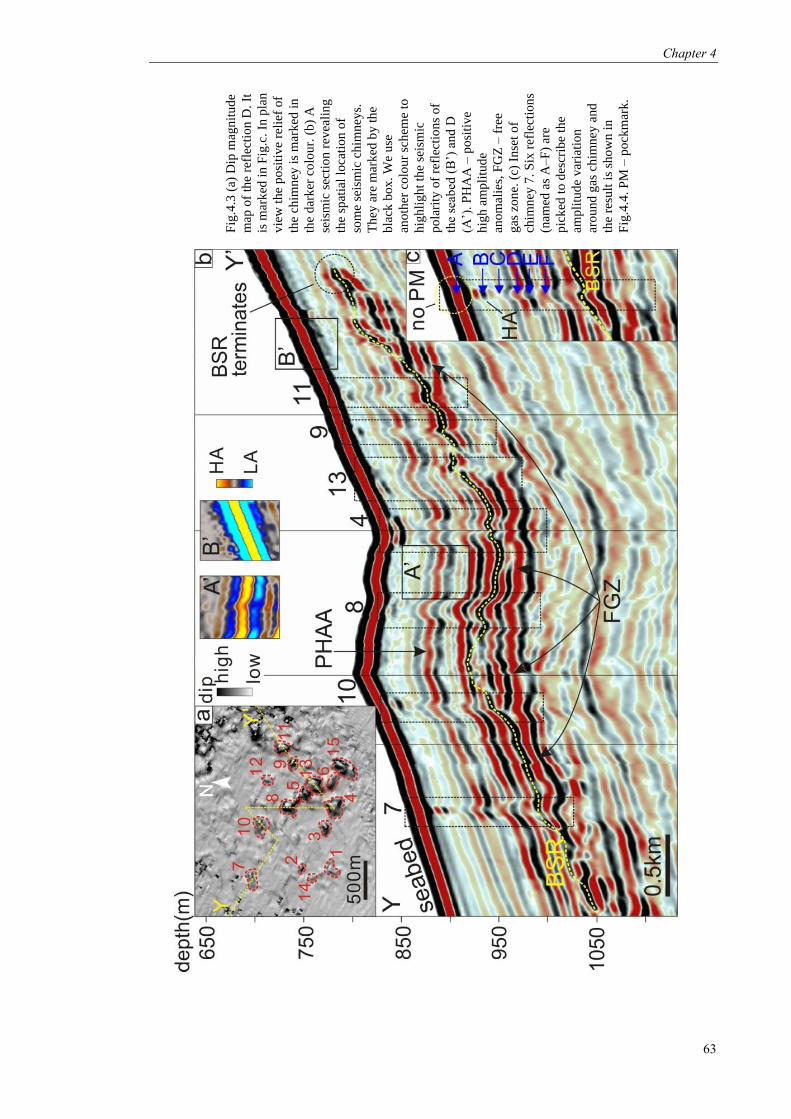
Chapter 4
63
Fig
.4.3
(a)
Dip
mag
nit
ud
e
map
of
the
refl
ecti
on D
. It
is m
ark
ed i
n F
ig.c
. In
pla
n
vie
w t
he
po
siti
ve
reli
ef o
f
the
chim
ney
is
mar
ked
in
the
dar
ker
co
lou
r. (
b)
A
seis
mic
sec
tio
n r
evea
lin
g
the
spat
ial
loca
tio
n o
f
som
e se
ism
ic c
him
ney
s.
Th
ey a
re m
ark
ed b
y t
he
bla
ck b
ox
. W
e u
se
ano
ther
co
lou
r sc
hem
e to
hig
hli
gh
t th
e se
ism
ic
po
lari
ty o
f re
flec
tio
ns
of
the
seab
ed (
B’)
and
D
(A’)
. P
HA
A –
po
siti
ve
hig
h a
mp
litu
de
ano
mal
ies,
FG
Z –
fre
e
gas
zo
ne.
(c)
In
set
of
chim
ney
7.
Six
ref
lect
ion
s
(nam
ed a
s A
–F
) ar
e
pic
ked
to
des
crib
e th
e
amp
litu
de
var
iati
on
aro
und
gas
ch
imn
ey a
nd
the
resu
lt i
s sh
ow
n i
n
Fig
.4.4
. P
M –
po
ckm
ark
.

Chapter 4
64
Fig.4.4 RMS amplitude map of the reflections A–F and the BSR (on the left). Their depths are marked
in Fig. 3c. Vertical black dotted lines indicate the spatial location of chimneys 7, 8, 10 and 12. PHAAs
at the reflection D and E (outlined by white dashed line) are identical and interpreted as hydrate
deposits. Note that the amplitude values in the reflection A (the seabed) are very high and its colour
scheme is different from others. The selected examples of the PHAAs are zoomed in (on the right).

Chapter 4
65
Fig
.4.5
Th
e m
od
elli
ng
res
ult
of
the
BH
SZ
dep
th v
ary
ing
wit
h t
ime
sin
ce t
he
LG
M.
Th
e sn
apsh
ots
at
thre
e ti
min
gs
(t1
-t3
) sh
ow
ho
w
the
hy
dra
te d
epo
sit
form
ed.
Th
e re
d t
rian
gle
mar
ks
the
loca
tio
n w
her
e th
e d
epth
of
the
BH
SZ
is
mo
del
led
in
app
end
ix 2
.
Chapter 5
66
Chapter 5 Gas venting that bypasses the feather edge of marine hydrate, offshore
Mauritania
Ang Li a, Richard J. Davies
b, Simon Mathias
a, Richard Hobbs
a, Miles Wilson
a
a Centre for Research into Earth Energy Systems (CeREES), Department of Earth Sciences,
Science Labs, Durham University, DH1 3LE, UK b School of Civil Engineering and Geosciences, Newcastle University, Newcastle upon Tyne,
Tyne and Wear, NE1 7RU, UK
Abstract:
Methane can be released from the vast marine hydrate reservoirs that surround continents into
oceans and potentially the atmosphere. But how these pathways work within the global carbon
cycle now and during a warmer world is only partially understood. Here we use 3-D seismic
data to identify what we interpret to be a venting system that bypasses the hydrate stability zone
(HSZ) offshore of Mauritania. This venting is manifested by the presence of the acoustic wipe-
out (AWO) across a densely faulted succession above a salt diapir and a set of morphological
features including a substantial, 260 m wide and 32 m deep, pockmark at the seabed. The base
of the HSZ is marked by a bottom simulating reflector (BSR) which deflects upwards above the
diapir, rather than mimicking the seabed. We use numerical modelling to show that this
deflection is caused by the underlying salt diapir. It creates a trapping geometry for gas sealed
by hydrate-clogged sediment. After entering the HSZ, some methane accumulated as hydrate in
the levees of a buried canyon. Venting in this locality probably reduces the flux of gas to the
landward limit of feather edge of hydrate, reducing the volume of gas that would be susceptible
for release during a warmer world.
Key words: gas hydrate, BSR, gas venting, diapir
Chapter 5
67
5.1 Introduction
Methane is a potent greenhouse gas and vast quantities of it are stored in marine hydrate,
a crystalline lattice of water and methane-dominated gas (Sloan and Koh, 2008). Its
susceptibility to ambient conditions makes it an unstable large carbon capacitor (Dickens, 2003;
Ruppel, 2011). Long-term atmospheric temperatures could change if a small proportion of
released gas entered the atmosphere (Archer et al., 2009). Therefore, understanding under what
circumstances methane can bypass hydrate-bearing sediment and enter the atmosphere is
important for assessing the impact of deep-buried methane on climatic change. Vigorous gas
plumes in which gas bubbles rise within clusters and reach sea surface before not all of these
gases are dissolved and oxidised in water body (McGinnis et al., 2006). This mechanism could
take place where effective venting systems operate.
The feeder system for the gas vents can be detected by seismic imaging and can take the
form of gas chimneys, which are vertically aligned reflections that probably represent clusters of
hydraulic fractures (Hovland and Judd, 1988; Cartwright et al., 2007). Gas-rich pore fluid can
be vented at different flux rates (Roberts, 2001). As a result, the morphological feature at the
seabed can be pockmarks (Moss and Cartwright, 2010), pingoes that host hydrate in the near-
seabed sediment (Serié et al., 2012) and mud volcanoes produced by the outflowing mud and
water (Milkov, 2000). Gas venting from these point sources constitutes an important part of the
known output of gas escaping from marine sediments (Judd, 2003).
Here we use 3-D seismic dataset to image what we interpret to be a venting system in
which gas bypasses a marine hydrate accumulation and pockmarks are distributed along leaking
faults. This provides a mechanism under which free gas could potentially reach shallow water.
What is unique here is the spatial relationship between the feather edge of marine hydrate and
the venting. Its presence prevents free gas from migrating landward, thus reducing the gas
located in the most vulnerable feather edge of hydrate that is susceptible to melting during
short-term ocean warming.

Chapter 5
68
5.2 Gas hydrate and feather edge
In deep-water settings gas hydrates can be revealed by a bottom simulating reflector
(BSR) in seismic reflection data. It marks the base of the hydrate stability zone (HSZ) and is
produced by an acoustic impedance contrast between sediments containing gas and hydrate
(Shipley et al., 1979; MacKay et al., 1994). This base shallows landwards until it intersects the
seabed and this zone is termed the feather edge, a critical site for understanding the dynamics of
marine hydrate (Ruppel, 2011; Berndt et al., 2014). Here ~3.5% of the global gas hydrate
inventory is trapped (Ruppel, 2011) and warming of bottom water can destabilise the near-
seafloor gas hydrate, which is evidenced by the presence of gas plumes (Skarke et al., 2014) and
predicted by numerical modelling (Phrampus and Hornbach, 2012). The released methane can
lead to ocean acidification and deoxygenation and perhaps climatic warming (Kvenvolden, 1993;
Archer et al., 2009; Biastoch et al., 2011).
5.3 Geological setting
The sedimentary features along the Mauritanian continental slope include canyon
channel systems, submarine slides and contourite moats (Krastel et al., 2006). The
sedimentation rates in different locations vary considerably (Krastel et al., 2006). Core samples
of up to 10 m long were recovered from GeoB 8509-2, GeoB 8520, GeoB 9624-1, GeoB 9623-2
and GeoB 9626-1 and show that the near-seabed deposit is predominately turbidite and hemi-
palegic sediments (Zühlsdorff et al., 2007; Henrich et al., 2008; Henrich et al., 2010).
Halokinesis is evidenced by the diapiric structures in a narrow elongate zone between 16 °N and
19 °N offshore the West Africa Continent and the age of the salt is probably Early Jurassic (Rad
et al., 1982). A salt diapir (located in 18°30’N, 16°50’W) has been revealed by the negative
Bouguer Anomaly. The study area is to the south of the Tioulit Canyon (Fig. 5.1). To the north
seismic features of complete feather edge have been recorded before (marked by yellow box in
Fig. 5.1a, Davies et al., 2015).

Chapter 5
69
Two wells, Chinguetti-6-1 and V-1, have been drilled within the 3-D seismic survey
and ~30 km north of the study area, confirming that the coastal basin of Mauritania is a potential
petroleum province and the Cenomanian-Turonian mudstones are able to generate hydrocarbons
(Vear, 2005). Seismic features linked to vertical gas migration include seismic chimneys
(Davies and Clarke, 2010) and large-scale gravity-driven faults (Yang and Davies, 2013). The
BSRs, either relict or modern ones, can be observed, which makes this site ideal to research
methane recycling in marine hydrate system (Davies and Clarke, 2010; Davies et al., 2012a).
5.4 Seismic dataset and methodology
The 3-D seismic data cover an area of ~4000 km2. They have been processed by
multiple suppression and post-stack time migration. The final bin spacing is 25 m × 25 m. These
data are displayed in two-way-travel time (TWTT). The velocity of succession investigated here
is likely to be ~1800 m/s and the dominant frequency of seismic data is ~50 Hz, which together
yield a vertical resolution of ~9 m. The positive acoustic impedance is recorded as a seismic
trough, which is a red-black loop in the seismic profile. A good example of the reflection having
such loop is the seabed one. The BSR is a black-red loop, consistent with a negative acoustic
impedance contrast. The seismic attributes used here are root mean square (RMS) amplitude and
dip magnitude. Both help identify bright spots (e.g. potential hydrocarbons) and structural
features (e.g. pockmarks and faults), respectively (Brown, 2010).
5.5 Observations
5.5.1 Fault system and seabed morphology
13 planar faults (named F1 to F13) with a NNW-SSE trend are identified on the basis of
clear offsets in stratal reflections (Fig. 5.1c). They all have a curved, concave-up geometry in
cross section (Fig. 5.1c, d). There are additional faults that are not so clearly imaged due to
acoustic wipe-out (AWO), particularly in the area bounded by F1, F2 and F4 (Fig. 5.2a, b). All
the faults are normal, though the throw of some of the faults is indiscernible at the seismic scale.
The faults have a similar angle of dip of ~50° and together form a crestal collapse graben

Chapter 5
70
system (Fig. 5.1c, d). The lower tip points of the faults are located at the top of a salt diapir (Fig.
5.1d). F1, F2 and F4, which are the major faults, have a throw of <10 ms (c. <9 m) near the
seabed and break surface whereas other faults tip out below the seabed (Fig. 5.1d). The spatial
correlation between the intruding diapir and the resultant faulting pattern has been seen in other
settings, for example offshore of North Carolina (Schmuck and Paull, 1993) and Angola (Serié
et al., 2012).
The morphological features at the seabed include fault scarps and a set of mounds and
depressions (Fig. 5.1b, Fig. 5.2). Four of them are selected for description here. Their
expression at the seabed varies from sub-circular to well-rounded (Fig. 5.2g-j). The long axis
ranges from 170 m to 410 m and the positive and negative deflections are ~27 – 53 m and ~32
m, respectively (Fig. 5.2). Their morphologies on the seismic profile are a symmetrical mound
(II, IV) or a depression (III), or the asymmetrical complex with a combination of both (I) (Fig.
5.2). The positive relief have a comparable morphology with the Arctic ice-cored hills in
Canada which are driven by growth of segregated ice or intrusion and progressive freezing of a
sub-pingo water lens (Mackay, 1987).
5.5.2 BSR and diapir
The BSR is identified based on the characteristic features of high seismic amplitude and
negative polarity over the area covered by the entire seismic dataset. In this case the BSR has a
geometry of an elongate, upward deflection that is analogous to an anticline (Fig. 5.3a), rather
than mimicking the seafloor in most cases (cf. offshore Oregon, Bangs et al., 2005). Along the
intersection between the faults and the BSR we identify some examples of positive relief of ~20
– 30 m in height (Fig. 5.2d and f, Fig. 5.3a). A salt diapir is ~1050 ms (c. 945 m) below seabed
and characterised by a chaotic internal seismic facies. Its top reflection is a red-black loop
representing the same polarity with seabed (Fig. 5.2). The diapir is elongated along the NNW-
SSE direction that is similar to the trend of the faults. Its hinge line is spatially coincident as the
region of maximum deflection of the BSR.
Chapter 5
71
The RMS amplitude map of the BSR displays some high-amplitude anomalies, most of
which are within the convex upward part of the BSR (Fig. 5.3b). These anomalies, which we
refer to as high-amplitude bands, have a crescent or linear geometry (Fig. 5.3b). Their strike
does not coincide with the depth contour of the BSR. Their width ranges from 150 m to 500 m.
For each band, the amplitude variation is symmetrical, with the highest amplitude in the middle
of the band and decreasing to both of its sides (Fig. 5.3b).
5.5.3 Positive high amplitude anomalies in levees
There are a set of ENE-WSW oriented buried canyons which have a low sinuosity (Fig.
5.3 and 5.4) above the BSR. These canyons have a multistory, aggradational and laterally offset
stacking pattern (Fig. 5.4a), which is similar to that of the channel-levee system in offshore Nile
delta (Catterall et al., 2010). The paleo-canyons are buried 50 – 65 ms (c. 45 – 58.5 m) below
the seabed and have a V-shaped cross-sectional morphology. The steepness of the canyon walls
decreases with decreasing burial depth. Sediments filling in the canyons have sub-horizontal
reflections (Fig. 5.4a). Three paleo-canyons are recognised and of our interest is the oldest one
that has a width of ~450 m in seismic cross section (marked in blue in Fig. 5.4a). The depth of
the channel ranges from 25 to 45 ms in TWTT (c. 22.5 – 40.5 m) and increases with water depth.
The thalweg trend is sub-parallel to the dip of the modern seabed (Fig. 5.3b). It bifurcates near
F1 (Fig. 5.4d), but the accurate location of divergence is unclear due to the overprinting effect
of the BSR.
The reflections, which downlap upon the paleo-seabed G (marked in orange dashed line
of Fig. 5.4a), are interpreted to represent sediments deposited in levee. Some positive high
amplitude anomalies (PHAAs) are found within these reflections. These PHAAs originate from
the place where the BSR intersects with F1 (Fig. 5.4c, d). They juxtapose F2 and fade out in an
up-dip direction (Fig. 5.4d). The amplitude map of reflection H shows that the PHAAs occur at
both flanks of the canyon, each with a wedge-like geometry (Fig. 5.4d). In plan view they are
bounded by the canyon wall and F2. The maximum value of the PHAA is largest near F2 and
the amplitude values decrease updip and also away from the canyon (Fig. 5.4d).

Chapter 5
72
5.6 Interpretation
5.6.1 Gas venting
AWO is a seismic response to gas filling in pores of sediment, which causes decrease of
P-wave velocity, severe ray bending, signal scattering and high transmission loss (Anderson and
Hampton, 1980). The result of signal lost or scattered is presented as acoustic fade-out or wipe-
out in the seismic cross section. The cores sampled as the shallow sediment in the Bering Sea
confirmed that AWO is caused by gas (Abrams, 1992). Therefore, we interpret that the AWO
zones, either ~200 m wide below the features of I–IV or km-scale wide ~300 m below the BSR
(Fig. 5.2), indicate the presence of free gases and escaping of gas along faults towards the
seabed.
The sub-circular depression (III, Fig. 5.2), which is a pockmark, suggests the
occurrence of venting of gas-rich pore fluid (Cartwright and Santamarina, 2015; Hovland and
Judd, 1988). The positive relief of I, II and IV could be the mud cone, the sediment of which is
unloaded onto the seabed after being transported vertically in a liquefied way (Dimitrov, 2002).
Their morphology is comparable to the mud volcanos found in the Gulf of Cadiz but of smaller
dimension (Somoza et al., 2003). The rate of the migration related to formation of mud cones is
documented to be fast (Roberts, 2001). Alternatively, the local up-bending of the seabed could
solely result from hydrate accretion, during which pore volume will expand due to the less
density of methane hydrate than that of seawater (Soloviev and Ginsburg; 1994). Such features,
named as pingos, were seen in offshore of Angola (90 – 300 m in extent and 5 – 40 m in height,
Serié et al., 2012) and Norwegian Sea (Hovland and Svensen, 2006), which were interpreted to
suggest seepage of hydrocarbon gas. Actually when focused fluid expulsion has a varying flux,
its expression at the seabed has a spectrum of features, rather than an exclusive one (Roberts,
2001; Roberts et al., 2006). In the venting system, the flux rate may vary with time and space,
thus it is likely that some features mentioned above may occur in a locale simultaneously and

Chapter 5
73
their seismic features could overprint on each other. Overall, the presence of these features
coupled with AWO is compelling evidence of gas bypassing the feather edge of marine hydrate.
5.6.2 Gases trapped below the BSR
In seismic reflection data high-amplitude bands (Fig. 5.3d) are a common seismic
response to the interface between hydrate-bearing sediments above the BSR and gas-bearing
sediments below it (Davies et al., 2015). Similar features have been described before by Li et al.
(2016) in the same seismic survey. Most of the bands here are within the upwarping region of
the BSR (Fig. 5.3b). The relief in the BSR creates a trapping geometry for free gas (Kvenvolden,
1993). Furthermore, under the eastern flank of the upwarping BSR we found a set of flat spots
(Fig. 5.3a), an evidence for the phase boundary between gas and water, or gas and oil (Brown,
2010). Therefore, we interpret that free gases are trapped below the BSR.
5.6.3 Hydrates hosted in levee sediment
Silty sand can be found in the cores sampled in levee successions near the seabed
(Henrich et al., 2010) and it potentially traps gas and hydrate stratigraphically. Hydrate filling in
pores of sediment can increase its acoustic impedance to the level such that it can be displayed
as enhanced reflections in seismic data because of a higher P-wave velocity of methane hydrate
(3750 – 3800 m/s, Helgerud et al., 2009). We interpret the PHAAs (marked in Fig. 5.4d) as an
isolated methane hydrate trap. The fact that the PHAAs have lower amplitude than the BSR
coincides with the synthetic seismic result which reveals that in marine sediment gas/hydrate
phase boundary normally has a higher acoustic impedance contrast than the hydrate/brine
interface (Zhang et al., 2012).
The amplitude variation of the PHAAs at reflection H may be the result of gas
migration. Based on the AWO, we interpret that gas breached the sealing at the level of BSR
near the intersection between faults and reflection H. If this gas could migrate along the levees,
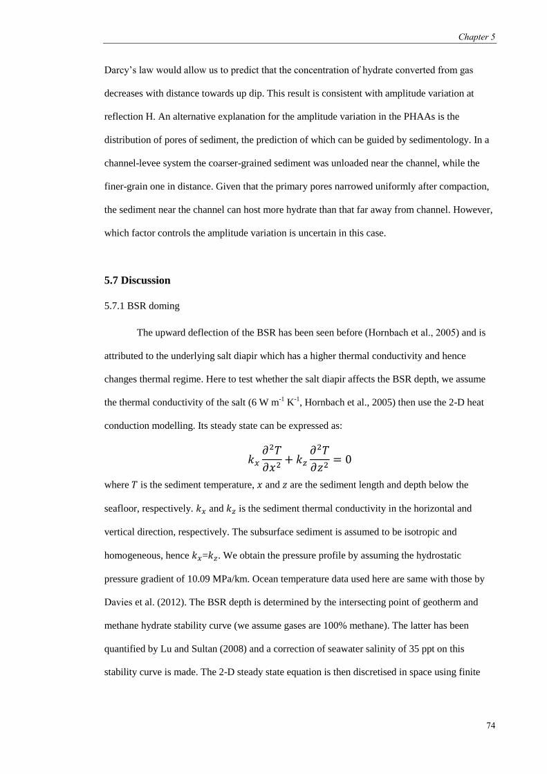
Chapter 5
74
Darcy’s law would allow us to predict that the concentration of hydrate converted from gas
decreases with distance towards up dip. This result is consistent with amplitude variation at
reflection H. An alternative explanation for the amplitude variation in the PHAAs is the
distribution of pores of sediment, the prediction of which can be guided by sedimentology. In a
channel-levee system the coarser-grained sediment was unloaded near the channel, while the
finer-grain one in distance. Given that the primary pores narrowed uniformly after compaction,
the sediment near the channel can host more hydrate than that far away from channel. However,
which factor controls the amplitude variation is uncertain in this case.
5.7 Discussion
5.7.1 BSR doming
The upward deflection of the BSR has been seen before (Hornbach et al., 2005) and is
attributed to the underlying salt diapir which has a higher thermal conductivity and hence
changes thermal regime. Here to test whether the salt diapir affects the BSR depth, we assume
the thermal conductivity of the salt (6 W m-1
K-1
, Hornbach et al., 2005) then use the 2-D heat
conduction modelling. Its steady state can be expressed as:
𝑘𝑥
𝜕2𝑇
𝜕𝑥2+ 𝑘𝑧
𝜕2𝑇
𝜕𝑧2= 0
where 𝑇 is the sediment temperature, 𝑥 and 𝑧 are the sediment length and depth below the
seafloor, respectively. 𝑘𝑥 and 𝑘𝑧 is the sediment thermal conductivity in the horizontal and
vertical direction, respectively. The subsurface sediment is assumed to be isotropic and
homogeneous, hence 𝑘𝑥=𝑘𝑧. We obtain the pressure profile by assuming the hydrostatic
pressure gradient of 10.09 MPa/km. Ocean temperature data used here are same with those by
Davies et al. (2012). The BSR depth is determined by the intersecting point of geotherm and
methane hydrate stability curve (we assume gases are 100% methane). The latter has been
quantified by Lu and Sultan (2008) and a correction of seawater salinity of 35 ppt on this
stability curve is made. The 2-D steady state equation is then discretised in space using finite

Chapter 5
75
differences and solved using MATLAB’s MLDIVIDE function. Any middle point of two
known neighbouring points A and B at either side of a boundary has a thermal conductivity 𝑘𝐴𝐵:
𝑘𝐴𝐵 = 2(1 𝑘𝐴⁄ + 1 𝑘𝐵⁄ )−1
where 𝑘𝐴 and 𝑘𝐵 is the thermal conductivity at point A and B, respectively. This modelling is
first used in the places where the BSR mimics the seabed to get the geothermal gradient fitting
best with the seismic observation (32oC km
-1), then in the study area.
The result shows that the modelled BSR has a good match with the observed one,
particularly across the crest of the diapir (Fig. 5.5). This implies that the salt diapir changed the
thermal regime and hence controls the geometry of the BSR. This increases the vertical relief of
the BSR and therefore the relief of the trap. We speculate that some of the local mismatches, in
particular the ones characterised by the local positive relief that is ~100 – 300 m wide adjacent
to some of the faults (marked by the right two black arrows in Fig. 5.5), may be caused by warm
focused flow that leads to local hydrate re-equilibrium (Crutchley et al., 2014). Therefore, the
BSR relocation is the result of heat transfer in the form of diffusion coupled with local
advection. However, there are some uncertainties that lead to the inaccuracy of the modelling
result. Salt carried by focused fluid along the faults, which is not considered in the model, may
increase the local salinity in the near-BSR sediment. Ionised salt can hinder hydration, leading
to the localised thinning of the HSZ (Sloan and Koh, 2008). Uncertainties in the modelled BSR
depths may also stem from error estimates of geothermal gradient, sediment conductivity,
velocity model in the subsurface and temperatures at the seabed.
5.7.2 Implication
In general, hydrate-bearing sediment is an effective barrier for free gas during its ascent
in the subsurface (Nimblett and Ruppel, 2003). Occasionally this gas can reach the seabed by
itself, such as when the pore pressure of its reservoir in a hydrate province reaches a level that
the fault slip can occur (Hornbach et al., 2004). Given that the trap created by the BSR
relocation is fully charged, the height of the gas column of the formed gas accumulation is

Chapter 5
76
estimated to be no more than 50 ms (c. 45 m). This height of gas column is significantly lower
than the critical height recorded in the Blake Ridge (~150 – 290 m, Hornbach et al., 2004).
Furthermore, we see no seismic evidence of the presence of thick free gas zone. This suggests
that the capillary entry pressure of overburden sediment along fault is lower than that of the
unfaulted sediment and this offers permeable route for gas to reach the seabed.
A BSR is present over the study area but mostly absent landward of it (Fig. 5.6a-c). This
is different from the area (marked in yellow box, Fig. 5.1a) to the north where sedimentary
context is similar but the BSR can be commonly observed (Davies et al., 2015). An explanation
for its absence landward is that methane venting above the diapir prevents landward gas
migration (Fig. 5.6d). Absence of free gas near the landward limit of the feather edge implies
less methane will be susceptible to being released in a warmer ocean in the future. Therefore,
diapirism could release methane into the ocean before it gets warmer and melts the marine
hydrate hosted in the sub-seabed sediment. Methane vented under this circumstance has high
flux rate when leaving the seabed and is likely to reach the shallow water or, possibly, the
atmosphere (McGinnis et al., 2006).
5.8 Conclusions
3-D seismic data provide compelling evidence for the occurrence of a gas venting
system, offshore Mauritania. A salt diapir provides the conditions to create migration pathways
for focused fluid of free gas that bypasses the feather edge of marine hydrate. The presence of
this system inhibits gas migration landward into the shallow feather edge region. This reduces
the volume of methane that would be susceptible to a warmer world in the future.

Chapter 5
77
5.9 Figures
Fig
.5.1
Ex
ten
t o
f th
e ar
ea c
over
ed
by
th
e 3
-D s
eism
ic s
urv
ey a
nd t
he
loca
tio
n o
f th
e st
ud
y a
rea.
Th
e
blu
e b
ox
of
soli
d l
ines
mar
ks
wh
ere
the
rela
tiv
ely
co
mp
lete
feat
her
edg
e w
as d
escr
ibed
by
Dav
ies
et a
l. (
20
15
). (
b)
Dip
-
mag
nit
ud
e m
ap o
f th
e se
abed
in
the
stu
dy
are
a sh
ow
ing
th
e fa
ult
scar
p a
nd
so
me
reli
efs
(nam
ed a
s
I, I
I, I
II a
nd
IV
). F
S –
fau
lt s
carp
.
Th
ere
are
som
e li
nea
r fe
ature
s
cau
sed
by
acq
uis
itio
n n
ois
e an
d
they
are
par
alle
l to
th
e in
lin
e
dir
ecti
on
. (c
) 3
-D i
mag
ing
of
the
fau
lts
(nam
ed a
s F
1–1
3)
fro
m t
op
vie
w.
Th
e w
hit
e ar
row
s m
ark
th
e
dis
pla
cem
ent
dir
ecti
on
of
the
han
gin
g w
all.
Ple
ase
no
te n
ot
all
the
fau
lts
term
inat
e at
th
e se
abed
.
(d)
A r
epre
sen
tati
ve
seis
mic
cro
ss
sect
ion
sh
ow
ing
th
e pat
tern
of
the
fau
lts
and
th
eir
spat
ial
rela
tio
nsh
ip
bet
wee
n t
he
un
der
lyin
g s
alt
dia
pir
.

Chapter 5
78
Fig
.5.2
(a–
b)
Rep
rese
nta
tiv
e se
ism
ic
cro
ss s
ecti
on
s
dis
pla
yin
g t
he
spat
ial
rela
tio
nsh
ip b
etw
een
th
e
reli
efs
at t
he
seab
ed,
the
fau
lts
and
th
e sa
lt
dia
pir
. T
he
aco
ust
ic
wip
ing
-ou
t (A
WO
)
sho
ws
up
bel
ow
I-I
V
and
in
th
e zo
ne
bo
un
ded
by
F1
, F
2 a
nd
F4
. (c
–f)
Zo
om
-in f
igure
s
sho
win
g t
he
cro
ss-
sect
ion
al g
eom
etry
of
I-
IV.
(g-j
) 3
-D i
mag
ing
of
the
bat
hy
met
ry
exh
ibit
ing
th
e
mo
rpho
logy
of
I-IV
.

Chapter 5
79
Fig.5.3 (a) A seismic cross section showing the upwarping section of the BSR. A different colour
scheme is used to highlight its polarity (cyan-yellow loop) that is opposite to that of the seabed
reflection (yellow-cyan loop). A flat spot is found under the upwarping BSR. Please note that this
figure is exaggerated vertically. HA – high amplitude, LA – low amplitude in this and subsequent
figures. (b) RMS amplitude map of the BSR. The white lines are the contours of the vertical distance
(measured in ms, TWTT) between the BSR and surface A. Surface A is an assumed planar surface and
on each cross line (E-W oriented) it is a segment defined by the down-dip (1, marked in inset) and the
up-dip point (2) along the BSR. The yellow dashed lines mark the outline of a buried old canyon and it
is described in section 5.6.3.
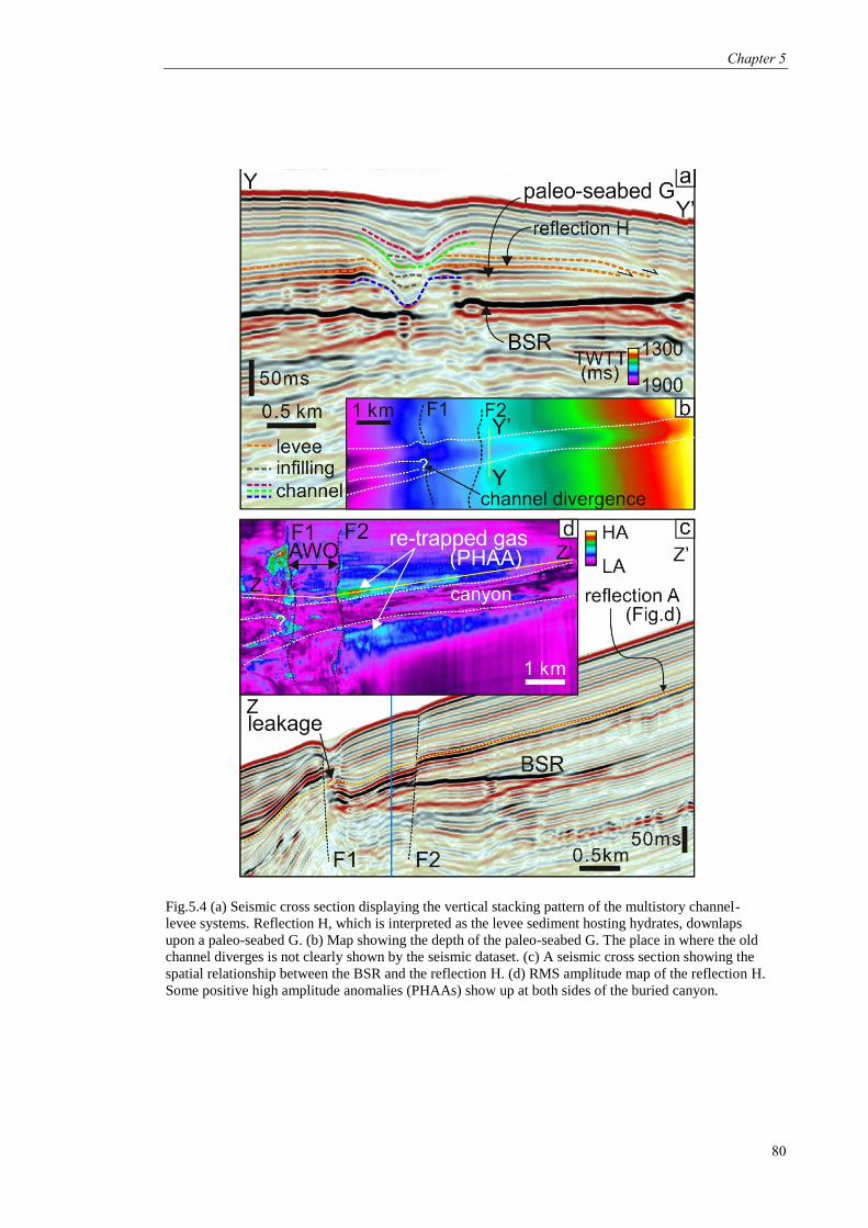
Chapter 5
80
Fig.5.4 (a) Seismic cross section displaying the vertical stacking pattern of the multistory channel-
levee systems. Reflection H, which is interpreted as the levee sediment hosting hydrates, downlaps
upon a paleo-seabed G. (b) Map showing the depth of the paleo-seabed G. The place in where the old
channel diverges is not clearly shown by the seismic dataset. (c) A seismic cross section showing the
spatial relationship between the BSR and the reflection H. (d) RMS amplitude map of the reflection H.
Some positive high amplitude anomalies (PHAAs) show up at both sides of the buried canyon.

Chapter 5
81
Fig.5.5 Modelling result of 2-D heat conduction. The black dashed line marks the top of the diapir. The
blue numbers indicate the temperature of each isothermal line. The black arrows mark the places where
there are some minor discrepancies between the modelled BSR and the observation result.
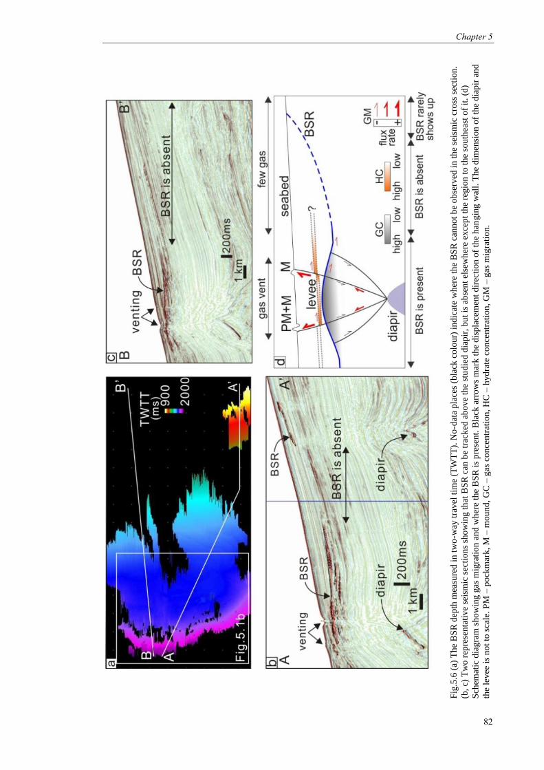
Chapter 5
82
Fig
.5.6
(a)
Th
e B
SR
dep
th m
easu
red
in
tw
o-w
ay t
rav
el t
ime
(TW
TT
). N
o-d
ata
pla
ces
(bla
ck c
olo
ur)
ind
icat
e w
her
e th
e B
SR
can
no
t b
e o
bse
rved
in
th
e se
ism
ic c
ross
sec
tio
n.
(b,
c) T
wo
rep
rese
nta
tiv
e se
ism
ic s
ecti
on
s sh
ow
ing
th
at B
SR
can
be
trac
ked
ab
ov
e th
e st
ud
ied
dia
pir
, b
ut
is a
bse
nt
else
wh
ere
exce
pt
the
reg
ion
to
th
e so
uth
east
of
it.
(d)
Sch
emat
ic d
iag
ram
sh
ow
ing
gas
mig
rati
on
and
wh
ere
the
BS
R i
s p
rese
nt.
Bla
ck a
rro
ws
mar
k t
he
dis
pla
cem
ent
dir
ecti
on o
f th
e h
ang
ing
wal
l. T
he
dim
ensi
on
of
the
dia
pir
an
d
the
lev
ee i
s n
ot
to s
cale
. P
M –
po
ckm
ark
, M
– m
oun
d,
GC
– g
as c
on
cen
trat
ion
, H
C –
hyd
rate
co
nce
ntr
atio
n,
GM
– g
as m
igra
tio
n.

Chapter 6
83
Chapter 6 Discussion and Conclusions
6.1 Uncertainties
6.1.1 Seismic resolution and interpretation
The vertical resolution of seismic data is commonly defined as one quarter of the
wavelength and it is uncertain in this research because there are no direct measurements of P-
wave velocity. The P-wave velocity in subsurface sediment is assumed to be 1800 m/s, but it
could be 1600 to 2000 m/s at <400 mbsf (Hustoft et al., 2009; Rajan et al., 2012). This causes
an error of ± 1 m in the vertical resolution, which is encountered in determining the height of
the gas column in chapter 3 and the total thickness of the hydrate-bearing sediments in chapter 4.
The uncertainties caused by solely using the seismic attribute of amplitude cannot be
eliminated but can be reduced by using appropriate rock physics tools (Avseth et al., 2010). The
seismic response of hydrate-bearing sediments could be either enhanced reflections (Hornbach
et al., 2003) or amplitude blanking (Lee et al., 1993). This uncertain seismic response may
cause difficulty in interpreting hydrate deposits. Here the 1-D synthetic seismogram is used to
discuss under what circumstances these responses will appear. The results (appendix 3) show
how a seismic waveform varies in response to hydrate-bearing sediments at different saturations
in the models of (a) an isolated hydrate in the HSZ and (b) hydrate-bearing sediments underlain
by free gas at the BSR (Fig.A3.1). For the model a, amplitude does not necessarily increase with
hydrate concentration. When the porosities of the hydrate reservoir and the clay are similar (e.g.
30% and 20%, Fig. A3.2), the amplitude responding to the interface between them increases
with hydrate concentration. When the hydrate concentration is 30% and the difference of these
porosities is 20% (Fig. A3.3), there is an apparent amplitude decrease at the interface. This
suggests that either amplitude blanking or enhanced reflectance can indicate the occurrence of
an isolated hydrate deposit. In addition, the absolute values of amplitude at the BSR are larger
than those at the clay-hydrate interface (Fig. A3.4), even if the hydrate concentration reaches
90%. This supports the interpretation of the hydrate deposits in chapter 4 and 5.

Chapter 6
84
6.1.2 Resetting of the BHSZ
When the BHSZ resets, driven by changes in ambient conditions, the magnitude of the
shoaling or deepening distance has a range and could vary at different sites. An example is
shown here (Fig. 6.1) to show the different resetting distances along the BHSZ in cross section.
A 2-D steady-state heat conduction model is used to estimate how much BHSZ should have
shoaled since the LGM. The governing equation and its solution are stated in section 5.7.1.
Input parameters, including the estimated present ocean temperature at this location and the
variation of the BWT and RSL are identical with those in chapter 4. The results (Fig. 6.1)
suggest that the vertical distance between the present-day BHSZ and the BHSZ during the LGM
decreases as the water depth reduces. In the 2-D heat diffusion model the BHSZ shoals by ~60
m (appendix 2) and this distance is larger than that estimated using the 2-D conduction method
here (39.1 m, the site is marked in dashed line in Fig. 6.1). The reason for the differences
between modelling results derives from the assumption of whether the thermal regime is at
steady state. Therefore, to compare resetting distance of the BHSZ between marine hydrate
systems around the world under the same circumstances, the modelling method and the site at
which this resetting occurs should be stated.
6.1.3 Parameters in modelling
The reliability of modelling outcome depends on to what degree the input parameters
are constrained (Harbaugh et al., 2001) and the method. In this research subsurface sediments
are assumed to be homogeneous and isotropic and this simplification fails to reveal complex
information, though it can accelerate computing of numerical models. An example is the
thermal conductivity in the models of 2-D heat conduction, which is assumed to be the same
along the horizontal (𝑥) and vertical (𝑧) directions. But in reality heat conduction in clastic
sediment is anisotropic such that 𝑘𝑥≠𝑘𝑧 (Ozisik, 1993). Secondly, some parameters, such as
BWT which in part controls the depth of the BHSZ, are not well constrained. Better
constraining the BWT requires analysis of isotopic records and is out of scope of this research.

Chapter 6
85
There are no direct measurements of past BWTs and therefore they are uncertain (Pekar et al.,
2002; Waelbroeck et al., 2002). Quantitatively assessing the impact of these uncertainties for the
modelling results is difficult solely by geophysical means. Another input parameter that has
uncertainty is the methane density. In chapter 3 the density of methane trapped below hydrates
is estimated under the assumption of being ideal gas, but actually it may be not. Peng-Robison
equation of state (EOS) is used to get the methane density and compare to that calculated using
Clapeyron equation. The results show that the density of ideal gas (100% methane) is ~28%
smaller (Fig. 6.2). The methane density is estimated to be 114 kg/m-3
at the pressure of 13.1
MPa, the temperature of 13 oC using Peng-Robison EOS. The proposed mechanism that
submarine failure can be primed is not affected after using this methane density but the critical
height of gas column would be 236 m instead of 231 m.
6.2 Discussion: responses of hydrates to changes in ambient conditions and fate of
released gas
The fundamental questions that this research attempts to answer are how methane in the
marine hydrate system migrates towards the seabed or is retained in the subsurface and how
marine hydrates along the continental margins behave during periods of ocean warming such as
since the LGM. The answers to these questions are important in assessing a series of proposed
consequences caused by methane release, including ocean deoxygenation and acidification
(Biastoch et al., 2011; Yamamoto et al., 2014) and, which is controversial, the climatic warming
(Kvenvolden, 1993; Kennett et al., 2000; Maslin et al., 2004; Myhre et al., 2016). Potential
scenarios for the fate of gases in the shallow (< 150 mbsf) and deep sections (≥ 150 mbsf) of the
feather edge of marine hydrates are discussed to comprehensively show the dynamics of marine
hydrates in the passive continental margin setting (Fig. 6.3). The depth of 150 mbsf is
determined arbitrarily to be the boundary between the deep and shallow section because at
places greater than this depth hydrates are relatively stable at a timescale of 100 yrs.

Chapter 6
86
In general there could be marine hydrates in the shallow section due to the feeding of
methane carried by upward fluid advection, though methane is normally oxidised anaerobically
by sulphate-consuming bacteria within the sediments that are < 70 mbsf (Borowski et al., 1999;
Ussler and Paull, 2008). Some photos taken by remotely operated vehicles at the seabed show
that gas hydrates occasionally occur at the seabed (e.g. Marcon et al., 2014). In the shallow
section of the study area few BSRs are observed in the seismic data. This could be explained by
that there are hydrates of low concentration underlain by few free gases, the configuration of
which could not produce detectable acoustic impedance contrast at the phase boundary (Mackay
et al., 1994; Davies et al., 2015). The small-scale presence of hydrates is also supported by the
potential outcropping gas hydrates imaged by the seismic data and these hydrates are located at
the irregular intersection between the BSR and the seabed (Fig. 6.3, Davies et al., 2015). Marine
hydrates in the shallow section are more susceptible to variations in ocean temperature.
Widespread methane release from the seabed, which is evidenced by gas plumes combined with
numerical models, has been documented, driven by the fluctuation of ocean temperature at the
timescales of one year (Berndt et al., 2014) and four decades (Westbrook et al., 2009; Hautala et
al., 2014). On the contrary, marine hydrates in the shallow section of the study area may not
release significant amounts of methane. The magnitude of the temperature change offshore of
Mauritania from 2009 to 2013 is < 1 oC (data from WOD). It results in that less marine hydrates
dissociated offshore Mauritania than those offshore West Spitsbergen (Westbrook et al., 2009)
and therefore less methane was released from the seabed offshore of Mauritania after 2009. The
seismic datasets show little evidence for hydrate dissociation and methane release from the
shallow section but this could be revealed by other data such as P-wave velocity (c.f. Sarkar et
al., 2012) and sonar images (c.f. Westbrook et al., 2009).
Gas hydrates in the deep section are more stable due to the relatively thick thermal
buffer of the overlying sediments in the HSZ (Archer et al., 2009). In the previous chapters
methane hydrate deposits are interpreted to be located at the base and in the HSZ, but not near
the seabed (Fig. 6.3). The formation of gas hydrates in the HSZ is often the result of advection
of methane (Pecher, 2002), which is supported by seismic features of vertical gas migration
conduits including faults and gas chimneys. The responses of gas hydrates at these sites have a

Chapter 6
87
longer delay due to heat conduction and can only respond to long-term (> 100 yrs) temperature
changes. Relative sea-level change is another factor that can extensively control the stability of
marine hydrates via affecting pore-fluid pressure (e.g. Crémière et al., 2016). In general the
depth of the BHSZ primarily depends on temperature and to a lesser extent on pressure
(Hornbach et al., 2008). For instance at the Blake Ridge, a 1 oC change in the geothermal
gradient and a 100 m change in the seafloor depth shift the depth of the BHSZ by ~15 m and ~5
m, respectively (water depth of 2800 m, seafloor temperature of 3.4 oC and thermal gradient of
34.3 oC/km, Sloan Jr and Koh, 2007; Hornbach et al., 2008). Therefore, marine hydrates along
the continental margin are more sensitive to ocean warming than sea-level rise over short term
(<1000 yrs) in the past. Once methane has been liberated from hydrates, it will not immediately
migrate through the effective barrier of the sub-seabed sediments. Instead, part of methane is
recycled when reaching the newly formed HSZ (Brown et al., 1996; Davies and Clarke, 2010).
Some other methane arriving at the BHSZ subsequently will be trapped below hydrate-bearing
sediments (Davies and Clarke, 2010; Minshull et al., 2016). There are some ways that gases can
bypass the impermeable sediment to reach the seabed: (a) accumulating gas below hydrates can
reduce the strength of the overlying sediments to the level that submarine failures could happen
(McIver, 1982; Li et al., 2016) then vast quantities of trapped gases will be released into the
ocean (McIver, 1982; Paull et al., 2002; Talling et al., 2014). It is proposed that multiple failures
could occur and this process may repeat itself before gas arriving at the seabed (Berndt et al.,
2012). (b) Critically pressured gas accumulation below hydrates could result in the formation of
vertical fractures (Davies and Clarke, 2010) and faults (Hornbach et al., 2004). Gases are
charged into and discharged from the sediments through these conduits at intervals, which
allows for episodic gas venting (Paull et al., 1995; Gorman et al., 2002; Crutchley et al., 2013).
The seismic datasets show that there are no submarine failures extending from the BHSZ to the
seabed and limited-scale substantial vents. Therefore, although some hydrates in the deep
section may be subject to the delayed thermal effect and probably dissociate recently, the
responses of hydrate to ambient conditions are slow and, more importantly, most of released
gases are retained in the subsurface. Even if gas could enter the ocean, most of it will be
oxidised during its ascent in the water column (McGinnis et al., 2006; Graves et al., 2015). Only
a small proportion of it could enter the atmosphere via catastrophic released of gas bubbles
coated by hydrates (McGinnis et al., 2006; Smith et al., 2014).

Chapter 6
88
6.3 Future work
Offshore of Mauritania is an underexplored region for marine hydrate and there are new
findings made in this research, but some fundamental questions with regard to marine hydrate
system are unanswered. For instance how much of methane released from hydrates can enter the
ocean and what is the proportion of this methane is retained in subsurface. Future work is
needed to continue elucidating the fate of methane released from and captured in marine hydrate
system offshore of Mauritania.
An upward shift of the BHSZ due to oceanic warming after the LGM is proposed, but
the evidence for the link to the LGM has uncertainties. Compelling evidence is needed to
corroborate the response of marine hydrate to temperature variation in the past. This response
has been researched around the world at the time scale of one year (Berndt et al., 2014) and
decades (Hautala et al., 2014) and during particular warming episodes, such as the Paleocene-
Eocene Thermal Maximum (PETM, Minshull et al., 2016) and the Early and Late Jurassic
(Hesselbo et al., 2000; Padden et al., 2001), but is still unclear in offshore of Mauritania. In the
last 8 years the fate of methane in the feather edge offshore of Mauritania can be examined by
taking the records of BWT in the World Ocean Database (WOD) as input parameters into the
numerical models. The results could allow for an estimation of the amount of released methane
and make the study area be a good example of short-term methane release at low-latitude
regions. In addition, offshore of Mauritania is an upwelling region and future work may provide
new insight into the flux rate of released methane in the context of deep ocean upwelling. To
better constrain the amount of released methane, the thickness and saturation of the hydrate
reservoir needs to be determined using seismic inversion and data from drilling (e.g. cores) with
proper rock physical tools.
Gas released by hydrate dissociation could cause submarine failures, ocean acidification
and deoxygenation. This gas would rise due to its buoyancy and attempt to reach a free surface
by either priming overlying sediment until failures happen (chapter 3) or bypassing the HSZ

Chapter 6
89
through gas chimneys (chapter 4) or along faults (chapter 5). After methane leaves the seabed,
how much of it will dissolve into the ocean and under what circumstances it can reach the
atmosphere or alternatively be recycled or oxidised are important in understanding its fate.
Answering these questions goes beyond the scope of this research but progress could be made if
any gas plume was found to sit right above a venting site in offshore of Mauritania. This could
be of help in knowing how much methane could enter the shallow waters and thus assessing its
impact.
6.4 Conclusions
Examining two exceptional-quality 3-D seismic surveys provides new insight into
marine hydrate system and gas migration in the subsurface offshore of Mauritania. The BSR,
which is an important tool to show the interface between hydrate-bearing and gas-charged
sediments, is identified on the basis of reflectance enhancement, reversed polarity and cross-
cutting stratal reflections. Linear high-amplitude features of different orientations at the level of
the BSR are found in both of the seismic surveys and termed ‘bands’. Their presence indicates
the widespread presence of free gases trapped stratigraphically below hydrates.
Hydrate dissociation is thought to be a possible trigger for submarine failures (e.g.
Storegga Slide offshore Norway, Sultan et al., 2004), as predicted by McIver (1982). His
hypothesis related to submarine failures includes another idea that buoyancy provided by gases
underlying hydrates could cause failures, which for the first time is supported by the seismic
evidence in this research. A seismically-imaged shear zone sits immediately above the BSR.
Buoyancy built up by the capped gas accumulation is calculated. It could prime the overlying
sediment for the incipient submarine failure, though it is uncertain to what degree gas-filled
pores within this gas accumulation are inter-connected.
The feather edge is an important site for warming-induced methane release into the
ocean (Westbrook et al., 2009; Phrampus and Hornbach, 2012). In this research a venting
Chapter 6
90
system was investigated and its existence is manifested by a series of pockmarks and mounds
aligning along permeable faults. Their spatial relationship together with acoustic wipe-out
indicates that gas-rich pore fluid bypasses the HSZ. The BHSZ at the feather edge is not marked
by a BSR everywhere. The BSR is absent because gases were vented rather than migrating
landwards along the BHSZ. Therefore, warming-induced methane release could not necessarily
take place at the landward limit of the feather edge in the study area.
Methane can be recycled as hydrates after being liberated from them. New evidence
involving some hydrate deposits fed by 15 gas chimneys indicates recycling could have
occurred. These hydrates are interpreted to form due to the thinning of the HSZ after the LGM.
This process implies that not all methane released from marine hydrates will necessarily enter
the ocean. Therefore, the contribution of marine hydrate to the atmospheric methane budget
could be less than that estimated before. Future work could focus on the amount of methane
transfer from the lithosphere to the hydrosphere at a given time scale and quantitatively assess
the implication of methane released from marine hydrate.

Chapter 6
91
6.5 Figures
Fig.6.1 The 2-D heat conduction modelling results of the BHSZ at present and the LGM. The upper
figure shows the distance between the two modelled BHSZs. The vertical dashed line marks the
position where 2-D heat diffusion model is adopted in chapter 4.
Fig.6.2 Methane densities at different depths. They are calculated using Clapeyron equation and Peng-
Robinson equation of state.

Chapter 6
92
Fig
. 6
.3 G
ener
ic d
iag
ram
sh
ow
ing
th
e m
arin
e h
yd
rate
sy
stem
off
sho
re o
f M
auri
tan
ia (
not
to s
cale
). T
he
upp
er s
ecti
on i
s a
mod
el f
or
the m
ech
anis
m p
ropo
sed
in
ch
apte
r 3
. A
sh
ear
zon
e is
o
bse
rved
alo
ng
th
e b
ase
of
hyd
rate
-fil
led
sed
imen
t. T
he
und
erly
ing
gas
co
uld
red
uce
th
e sh
ear
stre
ng
th o
f th
e h
yd
rate
-fil
led
sed
imen
t an
d p
rim
e th
e su
bm
arin
e fa
ilu
res.
Ex
cess
po
re p
ress
ure
co
uld
be
pre
serv
ed,
whic
h i
s su
ppo
rted
by
th
at n
o g
as c
him
ney
s b
reac
h t
he
BS
R s
eali
ng
in
th
e sh
ear
zon
e. T
he
mid
dle
sec
tio
n s
ho
ws
the
ven
ting
sy
stem
sta
ted
in
ch
apte
r 5
. G
as m
igra
ted
alo
ng t
he
dia
pir
ism
-dri
ven
fau
lt, b
yp
asse
d t
he
HS
Z a
nd
en
tere
d t
he
oce
an,
leav
ing
th
e m
ou
nd
s an
d p
ock
mar
ks
at t
he
seab
ed.
Du
e to
this
ven
t, l
ater
al g
as m
igra
tio
n i
s in
terc
epte
d a
nd
th
e B
SR
ca
nn
ot
be
ob
serv
ed l
and
war
d o
f th
e v
enti
ng s
yst
em.
Th
e lo
wer
sec
tio
n s
um
mar
ises
th
e in
terp
reta
tio
ns
in c
hap
ter
4 a
nd
oth
ers
that
are
no
t st
ated
in p
rev
iou
s ch
apte
rs.
Met
han
e is
rec
ycl
ed a
s g
as h
yd
rate
aft
er e
nte
ring
th
e H
SZ
. T
he
cany
on
aff
ects
th
e lo
cati
on
of
the
BH
SZ
an
d a
llo
ws
gas
to
mig
rate
lat
eral
ly a
lon
g t
he
can
yon
wal
l. T
he
inte
rsec
tio
n o
f th
e B
HS
Z a
nd t
he
seab
ed i
s ir
reg
ula
r an
d a
lon
g i
t p
ock
mar
ks
and
ou
tcro
pp
ing h
yd
rate
s ca
n b
e fo
und
.

References
93
References
Abrams, M.A., 1992. Geophysical and geochemical evidence for subsurface hydrocarbon
leakage in the Bering Sea, Alaska. Marine and Petroleum Geology 9(2), 208-221.
Anderson, A.L., Hampton, L.D., 1980. Acoustics of gas-bearing sediments I. Background. The
Journal of the Acoustical Society of America 67(6), 1865-1889.
Andreassen, K., Hart, P.E., MacKay, M., 1997. Amplitude versus offset modeling of the bottom
simulating reflection associated with submarine gas hydrates. Marine Geology 137(1-2),
25-40.
Andreassen, K., Mienert, J., Bryn, P., Singh, S.C., 2000. A double gas-hydrate related bottom
simulating reflector at the Norwegian continental margin. Annals of the New York
Academy of Sciences 912(1), 126-135.
Andresen, K.J., Huuse, M., Schodt, N.H., Clausen, L.F., Seidler, L., 2011. Hydrocarbon
plumbing systems of salt minibasins offshore Angola revealed by three-dimensional
seismic analysis. AAPG bulletin 95(6), 1039-1065.
Antobreh, A.A., Krastel, S., 2006. Morphology, seismic characteristics and development of Cap
Timiris Canyon, offshore Mauritania: a newly discovered canyon preserved-off a major
arid climatic region. Marine and Petroleum Geology 23(1), 37-59.
Antobreh, A.A., Krastel, S., 2007. Mauritania Slide Complex: morphology, seismic
characterisation and processes of formation. International Journal of Earth Sciences
96(3), 451-472.
Archer, D., Buffett, B., Brovkin, V., 2009. Ocean methane hydrates as a slow tipping point in
the global carbon cycle. Proceedings of the National Academy of Sciences 106(49),
20596-20601.
Avseth, P., Mukerji, T., Mavko, G., 2010. Quantitative seismic interpretation: Applying rock
physics tools to reduce interpretation risk. Cambridge university press, 168.
Bacon, M., Simm, R., Redshaw, T., 2007. 3-D seismic interpretation. Cambridge University
Press, 18-55.
Bangs, N.L., Musgrave, R.J., Tréhu, A.M., 2005. Upward shifts in the southern Hydrate Ridge
gas hydrate stability zone following postglacial warming, offshore Oregon. Journal of
Geophysical Research: Solid Earth 110, B03102, doi:10.1029/2004JB003293.
Beaudoin, Y.C., Dallimore, S.R., Boswell, R., 2014. Frozen heat: A UNEP global outlook on
methane gas hydrates. United Nations Environment Programme, GRID-Arendal, 29.
Berndt, C., Feseker, T., Treude, T., Krastel, S., Liebetrau, V., Niemann, H., Bertics, V.J.,
Dumke, I., Dünnbier, K., Ferré, B., 2014. Temporal constraints on hydrate-controlled
methane seepage off Svalbard. Science 343(6168), 284-287.
Berndt, C., Costa, S., Canals, M., Camerlenghi, A., de Mol, B., Saunders, M., 2012. Repeated
slope failure linked to fluid migration: The Ana submarine landslide complex, Eivissa
Channel, Western Mediterranean Sea. Earth and Planetary Science Letters 319, 65-74.
References
94
Berndt, C., Mienert, J., Vanneste, M., Bünz, S., Bryn, P., 2002. Submarine slope-failure
offshore Norway triggers rapid gas hydrate decomposition, Proceedings of the Fourth
International Conference on Gas Hydrates, Yokohama, Japan, 19-23, May, 71-74.
Biastoch, A., Treude, T., Rüpke, L.H., Riebesell, U., Roth, C., Burwicz, E.B., Park, W., Latif,
M., Böning, C.W., Madec, G., 2011. Rising Arctic Ocean temperatures cause gas
hydrate destabilization and ocean acidification. Geophysical Research Letters 38,
L08602, doi:10.1029/2011GL047222.
Bintanja, R., Van de Wal, R., 2008. North American ice-sheet dynamics and the onset of
100,000-year glacial cycles. Nature 454(7206), 869-872.
Boait, F., White, N., Bickle, M., Chadwick, R., Neufeld, J., Huppert, H., 2012. Spatial and
temporal evolution of injected CO2 at the Sleipner Field, North Sea. Journal of
Geophysical Research: Solid Earth 117, B03309, doi:10.1029/2011JB008603.
Booth, J.S., Winters, W.J., Dillon, W.P., 1994. Circumstantial Evidence of Gas Hydrate and
Slope Failure Associations on the United-States Atlantic Continental-Margin. Annals of
the New York Academy of Sciences 715(1), 487-489.
Borowski, W.S., Paull, C.K., Ussler, W., 1999. Global and local variations of interstitial sulfate
gradients in deep-water, continental margin sediments: Sensitivity to underlying
methane and gas hydrates. Marine Geology 159(1), 131-154.
Boswell, R., 2009. Is gas hydrate energy within reach? Science 325(5943), 957-958.
Boswell, R., Collett, T.S., 2011. Current perspectives on gas hydrate resources. Energy &
Environmental Science 4(4), 1206-1215.
Brooks, J., Kennicutt, M., Fay, R., McDonald, T., Sassen, R., 1984. Thermogenic gas hydrates
in the Gulf of Mexico. Science 225(4660), 409-411.
Brown, A., 2010, Interpretation of Three-dimensional Seismic Data, seventh ed., AAPG and
EGP, Tulsa, 31-60, 275-281.
Brown, H.E., Holbrook, W.S., Hornbach, M.J., Nealon, J., 2006. Slide structure and role of gas
hydrate at the northern boundary of the Storegga Slide, offshore Norway. Marine
Geology 229(3), 179-186.
Brown, K.M., Bangs, N.L., Froelich, P.N., Kvenvolden, K.A., 1996. The nature, distribution,
and origin of gas hydrate in the Chile Triple Junction region. Earth and Planetary
Science Letters 139(3-4), 471-483.
Bull, S., Cartwright, J., Huuse, M., 2009a. A review of kinematic indicators from mass-transport
complexes using 3D seismic data. Marine and Petroleum Geology 26(7), 1132-1151.
Bull, S., Cartwright, J., Huuse, M., 2009b. A subsurface evacuation model for submarine slope
failure. Basin Research 21(4), 433-443.
Bünz, S., Mienert, J., 2004. Acoustic imaging of gas hydrate and free gas at the Storegga Slide.
Journal of Geophysical Research: Solid Earth 109, B04102, doi:10.1029/
2003JB002863.

References
95
Bünz, S., Mienert, J., Bryn, P., Berg, K., 2005. Fluid flow impact on slope failure from 3D
seismic data: a case study in the Storegga Slide. Basin Research 17(1), 109-122.
Bünz, S., Polyanov, S., Vadakkepuliyambatta, S., Consolaro, C., Mienert, J., 2012. Active gas
venting through hydrate-bearing sediments on the Vestnesa Ridge, offshore W-Svalbard.
Marine Geology 332, 189-197.
Carcione, J.M., Tinivella, U., 2000. Bottom-simulating reflectors: Seismic velocities and AVO
effects. Geophysics 65(1), 54-67, doi:10.1190/1.1444725.
Cartwright, J., 2007. The impact of 3D seismic data on the understanding of compaction, fluid
flow and diagenesis in sedimentary basins. Journal of the Geological Society 164(5),
881-893.
Cartwright, J., Huuse, M., Aplin, A., 2007. Seal bypass systems. AAPG Bulletin 91(8), 1141-
1166.
Cartwright, J., Santamarina, C., 2015. Seismic characteristics of fluid escape pipes in
sedimentary basins: Implications for pipe genesis. Marine and Petroleum Geology 65,
126-140.
Cathles, L.M., Su, Z., Chen, D., 2010. The physics of gas chimney and pockmark formation,
with implications for assessment of seafloor hazards and gas sequestration. Marine and
Petroleum Geology 27(1), 82-91.
Catterall, V., Redfern, J., Gawthorpe, R., Hansen, D., Thomas, M., 2010. Architectural style and
quantification of a submarine channel–levee system located in a structurally complex
area: offshore Nile Delta. Journal of Sedimentary Research 80(11), 991-1017.
Chabert, A., Minshull, T.A., Westbrook, G.K., Berndt, C., Thatcher, K.E., Sarkar, S., 2011.
Characterization of a stratigraphically constrained gas hydrate system along the western
continental margin of Svalbard from ocean bottom seismometer data. Journal of
Geophysical Research: Solid Earth 116, B12102, doi:10.1029/2011JB008211.
Chappellaz, J.A., Fung, I.Y., Thompson, A.M., 1993. The atmospheric CH4 increase since the
Last Glacial Maximum. Tellus B 45, 228-241, doi:10.1034/j.1600-0889.1993.t01-2-
00002.x.
Clennell, M.B., Hovland, M., Booth, J.S., Henry, P., Winters, W.J., 1999. Formation of natural
gas hydrates in marine sediments: 1. Conceptual model of gas hydrate growth
conditioned by host sediment properties. Journal of Geophysical Research: Solid Earth
104(B10), 22985–23003, doi:10.1029/1999JB900175.
Collett, T., 1999. Detailed evaluation of gas hydrate reservoir properties using
JAPEX/JNOC/GSC Mallik 2L-38 gas hydrate research well downhole well-log displays.
Bulletin of the Geological Survey of Canada, 295-311.
Collett, T.S., 2001. A review of well-log analysis techniques used to assess gas-hydrate-bearing
reservoirs. Natural gas hydrates: occurrence, distribution, and detection, 189-210.
Collett, T.S., 2002. Energy resource potential of natural gas hydrates. AAPG Bulletin 86(11),
1971-1992.

References
96
Collett, T.S., 2008. Assessment of gas hydrate resources on the North Slope, Alaska, 2008.
AGU Fall Meeting Abstracts, 2008AGUFMOS43F..08C.
Collett, T.S., Wendlandt, R.F., 2000. Formation evaluation of gas hydrate-bearing marine
sediments on the Blake Ridge with downhole geochemical log measurements,
Proceedings of the Ocean Drilling Program, Scientific Results 164, 199-215.
Crémière, A., Lepland, A., Chand, S., Sahy, D., Condon, D.J., Noble, S.R., Martma, T.,
Thorsnes, T., Sauer, S., Brunstad, H., 2016. Timescales of methane seepage on the
Norwegian margin following collapse of the Scandinavian Ice Sheet. Nature
communications 7.
Crutchley, G.J., Berndt, C., Geiger, S., Klaeschen, D., Papenberg, C., Klaucke, I., Hornbach,
M.J., Bangs, N.L., Maier, C., 2013. Drivers of focused fluid flow and methane seepage
at south Hydrate Ridge, offshore Oregon, USA. Geology 41(5), 551-554.
Crutchley, G.J., Klaeschen, D., Planert, L., Bialas, J., Berndt, C., Papenberg, C., Hensen, C.,
Hornbach, M., Krastel, S., Brückmann, W., 2014. The impact of fluid advection on gas
hydrate stability: Investigations at sites of methane seepage offshore Costa Rica. Earth
and Planetary Science Letters 401, 95-109.
Davie, M.K., Buffett, B.A., 2003. Sources of methane for marine gas hydrate: inferences from a
comparison of observations and numerical models. Earth and Planetary Science Letters
206(1), 51-63.
Davies, R.J., Clarke, A.L., 2010. Methane recycling between hydrate and critically pressured
stratigraphic traps, offshore Mauritania. Geology 38(11), 963-966.
Davies, R.J., Thatcher, K.E., Armstrong, H., Yang, J., Hunter, S., 2012a. Tracking the relict
bases of marine methane hydrates using their intersections with stratigraphic reflections.
Geology 40(11), 1011-1014.
Davies, R.J., Thatcher, K.E., Mathias, S.A., Yang, J., 2012b. Deepwater canyons: An escape
route for methane sealed by methane hydrate. Earth and Planetary Science Letters 323,
72-78.
Davies, R.J., Yang, J., Hobbs, R., Li, A., 2014. Probable patterns of gas flow and hydrate
accretion at the base of the hydrate stability zone. Geology 42(12), 1055-1058.
Davies, R.J., Yang, J., Li, A., Mathias, S., Hobbs, R., 2015. An irregular feather-edge and
potential outcrop of marine gas hydrate along the Mauritanian margin. Earth and
Planetary Science Letters 423, 202-209.
Dickens, G.R., 2003. Rethinking the global carbon cycle with a large, dynamic and microbially
mediated gas hydrate capacitor. Earth and Planetary Science Letters 213(3), 169-183.
Dickens, G.R., Paull, C.K., Wallace, P., 1997. Direct measurement of in situ methane quantities
in a large gas-hydrate reservoir. Nature 385, 426-428.
Dillon, W.P., Nealon, J.W., Taylor, M.H., Lee, M.W., Drury, R.M., Anton, C.H., 2001. Seafloor
collapse and methane venting associated with gas hydrate on the blake ridge: causes and
implications to seafloor stability and methanerelease. Natural gas hydrates: occurrence,
distribution, and detection, 211-233.

References
97
Dimitrov, L.I., 2002. Mud volcanoes – the most important pathway for degassing deeply buried
sediments. Earth-Science Reviews 59(1), 49-76.
Egorov, A.V., Rozhkov, A.N., 2010. Formation of gas hydrate reservoirs in submarine mud
volcanos. Fluid Dynamics 45(5), 769-778.
Flemings, P.B., Liu, X.L., Winters, W.J., 2003. Critical pressure and multiphase flow in Blake
Ridge gas hydrates. Geology 31(12), 1057-1060.
Ford, K., Naehr, T., Skilbeck, G., 2003. The use of infrared thermal imaging to identify gas
hydrate in sediment cores, Proceedings of the Ocean Drilling Program, Scientific
results. Ocean Drilling Program, Texas A&M University, initial reports volume 201.
Foucher, J.P., Nouzé, H., Henry, P., 2002. Observation and tentative interpretation of a double
BSR on the Nankai slope. Marine Geology 187(1), 161-175.
Gay, A., Lopez, M., Cochonat, P., Seranne, M., Levache, D., Sermondadaz, G., 2006. Isolated
seafloor pockmarks linked to BSRs, fluid chimneys, polygonal faults and stacked
Oligocene-Miocene turbiditic palaeochannels in the Lower Congo Basin. Marine
Geology 226(1), 25-40.
Ginsburg, G., Soloviev, V., Cranston, R., Lorenson, T., Kvenvolden, K., 1993. Gas hydrates
from the continental slope, offshore Sakhalin Island, Okhotsk Sea. Geo-Marine Letters
13(1), 41-48.
Golmshtok, A.Y., Soloviev, V.A., 2006. Some remarks on the thermal nature of the double BSR.
Marine Geology 229(3), 187-198.
Gorman, A.R., Holbrook, W.S., Hornbach, M.J., Hackwith, K.L., Lizarralde, D., Pecher, I.,
2002. Migration of methane gas through the hydrate stability zone in a low-flux hydrate
province. Geology 30(4), 327-330.
Gornitz, V., Fung, I., 1994. Potential distribution of methane hydrates in the world's oceans.
Global Biogeochemical Cycles 8(3), 335-347.
Graves, C.A., Steinle, L., Rehder, G., Niemann, H., Connelly, D.P., Lowry, D., Fisher, R.E.,
Stott, A.W., Sahling, H., James, R.H., 2015. Fluxes and fate of dissolved methane
released at the seafloor at the landward limit of the gas hydrate stability zone offshore
western Svalbard. Journal of Geophysical Research: Oceans 120, 6185-6201,
doi:10.1002/2015JC011084.
Haacke, R.R., Westbrook, G.K., Hyndman, R.D., 2007. Gas hydrate, fluid flow and free gas:
Formation of the bottom-simulating reflector. Earth and Planetary Science Letters
261(3), 407-420.
Harbaugh, J.W., Merriam, D.F., Davis, J.C., 2001. Geologic modeling and simulation:
sedimentary systems. Springer Science & Business Media, 135.
Harvey, L., Huang, Z., 1995. Evaluation of the potential impact of methane clathrate
destabilization on future global warming. Journal of Geophysical Research:
Atmospheres 100(D2), 2905-2926, doi:10.1029/94JD02829.
References
98
Hautala, S.L., Solomon, E.A., Johnson, H.P., Harris, R.N., Miller, U.K., 2014. Dissociation of
Cascadia margin gas hydrates in response to contemporary ocean warming.
Geophysical Research Letters 41, 8486-8494, doi:10.1002/2014GL061606.
Helgerud, M., Waite, W.F., Kirby, S., Nur, A., 2009. Elastic wave speeds and moduli in
polycrystalline ice Ih, sI methane hydrate, and sII methane-ethane hydrate. Journal of
Geophysical Research: Solid Earth 114, B02212, doi:10.1029/2008JB006132.
Henrich, R., Cherubini, Y., Meggers, H., 2010. Climate and sea level induced turbidite activity
in a canyon system offshore the hyperarid Western Sahara (Mauritania): The Timiris
Canyon. Marine Geology 275(1), 178-198.
Henrich, R., Hanebuth, T.J.J., Krastel, S., Neubert, N., Wynn, R.B., 2008. Architecture and
sediment dynamics of the Mauritania Slide Complex. Marine and Petroleum Geology
25(1), 17-33.
Hesse, R., Harrison, W.E., 1981. Gas hydrates (clathrates) causing pore-water freshening and
oxygen isotope fractionation in deep-water sedimentary sections of terrigenous
continental margins. Earth and Planetary Science Letters 55(3), 453-462.
Hesselbo, S.P., Gröcke, D.R., Jenkyns, H.C., Bjerrum, C.J., Farrimond, P., Bell, H.S.M., Green,
O.R., 2000. Massive dissociation of gas hydrate during a Jurassic oceanic anoxic event.
Nature 406(6794), 392-395.
Ho, S., Cartwright, J.A., Imbert, P., 2012. Vertical evolution of fluid venting structures in
relation to gas flux, in the Neogene-Quaternary of the Lower Congo Basin, Offshore
Angola. Marine Geology 332, 40-55.
Hoehler, T.M., Borowski, W.S., Alperin, M.J., Rodriguez, N.M., Paull, C.K., 2000. Model,
stable isotope, and radiotracer characterization of anaerobic methane oxidation in gas
hydrate-bearing sediments of the Blake Ridge, Proceedings of the Ocean Drilling
Program, Scientific Results. Ocean Drilling Program College Station, TX, 79-85.
Hornbach, M.J., Holbrook, W.S., Gorman, A.R., Hackwith, K.L., Lizarralde, D., Pecher, I.,
2003. Direct seismic detection of methane hydrate on the Blake Ridge. Geophysics
68(1), 92-100, doi: 10.1190/1.1543196
Hornbach, M.J., Ruppel, C., Saffer, D.M., Van Dover, C.L., Holbrook, W.S., 2005. Coupled
geophysical constraints on heat flow and fluid flux at a salt diapir. Geophysical
Research Letters 32, L24617, doi:10.1029/2005GL024862.
Hornbach, M.J., Saffer, D.M., Holbrook, W.S., 2004. Critically pressured free-gas reservoirs
below gas-hydrate provinces. Nature 427(6970), 142-144.
Hornbach, M.J., Saffer, D.M., Holbrook, W.S., Van Avendonk, H.J., Gorman, A.R., 2008.
Three-dimensional seismic imaging of the Blake Ridge methane hydrate province:
Evidence for large, concentrated zones of gas hydrate and morphologically driven
advection. Journal of Geophysical Research: Solid Earth 113, B07101,
doi:10.1029/2007JB005392.
Horozal, S., Bahk, J.J., Urgeles, R., Kim, G.Y., Cukur, D., Kim, S.P., Lee, G.H., Lee, S.H., Ryu,
B.J., Kim, J.H., 2017. Mapping gas hydrate and fluid flow indicators and modeling gas
References
99
hydrate stability zone (GHSZ) in the Ulleung Basin, East (Japan) Sea: Potential linkage
between the occurrence of mass failures and gas hydrate dissociation. Marine and
Petroleum Geology 80, 171-191.
Houghton, J.T., Callander, B.A., Varney, S.K., 1992. The supplementary report to the IPCC
scientific assessment. Intergovernmental Panel on Cllmate Change, Cambrldge Univ
Press, Cambridge, 29.
Hovland, M., Judd, A., 1988. Seabed pockmarks and seepages: impact on geology, biology, and
the marine environment. Springer, 119-131.
Hovland, M., Svensen, H., 2006. Submarine pingoes: Indicators of shallow gas hydrates in a
pockmark at Nyegga, Norwegian Sea. Marine Geology 228(1), 15-23.
Hovland, M., Talbot, M.R., Qvale, H., Olaussen, S., Aasberg, L., 1987. Methane-related
carbonate cements in pockmarks of the North Sea. Journal of Sedimentary Research
57(5), 881-892.
Hunter, S.J., Goldobin, D.S., Haywood, A.M., Ridgwell, A., Rees, J.G., 2013. Sensitivity of the
global submarine hydrate inventory to scenarios of future climate change, Earth and
Planetary Science Letters 367, 105-115, doi:10.1016/j.epsl.2013.02.017.
Hustoft, S., Bünz, S., Mienert, J., 2010. Three-dimensional seismic analysis of the morphology
and spatial distribution of chimneys beneath the Nyegga pockmark field, offshore mid-
Norway. Basin Research 22(4), 465-480.
Hustoft, S., Bünz, S., Mienert, J., Chand, S., 2009. Gas hydrate reservoir and active methane-
venting province in sediments on < 20 Ma young oceanic crust in the Fram Strait,
offshore NW-Svalbard. Earth and Planetary Science Letters 284(1), 12-24.
Hustoft, S., Mienert, J., Bunz, S., Nouze, H., 2007. High-resolution 3D-seismic data indicate
focussed fluid migration pathways above polygonal fault systems of the mid-Norwegian
margin. Marine Geology 245(1), 89-106.
Ivanov, M., Blinova, V., Kozlova, E., Westbrook, G., Mazzini, A., Minshull, T., Nouzé, H.,
2007. First sampling of gas hydrate from the Vøring Plateau. Eos, Transactions
American Geophysical Union 88(19), 209-216.
Jaeger, J.C., Cook, N.G., Zimmerman, R., 2009. Fundamentals of rock mechanics. John Wiley
& Sons, 90-94.
Johnson, A.H., 2011. Global resource potential of gas hydrate – a new calculation. Natural Gas
& Oil 304, 285-4541.
Judd, A.G., 2003. The global importance and context of methane escape from the seabed. Geo-
Marine Letters 23(3-4), 147-154.
Kennett, J.P., Cannariato, K.G., Hendy, I.L., Behl, R.J., 2000. Carbon isotopic evidence for
methane hydrate instability during Quaternary interstadials. Science 288(5463), 128-133.
Kennett, J.P., Cannariato, K.G., Hendy, I.L., Behl, R.J., 2003. Methane hydrates in quaternary
climate change: the clathrate gun hypothesi. Spec. Publ. American Geophysical Union,
Washington, DC, 1-9.

References
100
Kerr, R.A., 2004. Gas hydrate resource: smaller but sooner. Science 303(5660), 946-947.
Krastel, S., Wynn, R.B., Hanebuth, T.J.J., Henrich, R., Holz, C., Meggers, H., Kuhlmann, H.,
Georgiopoulou, A., Schulz, H.D., 2006. Mapping of seabed morphology and shallow
Sediment structure of the Mauritania continental margin, Northwest Africa: some
implications for geohazard potential. Norwegian Journal of Geology 86, 163-176.
Krustel, S., Wynn, R.B., Honebuth, T., Henrich, R., Holz, C., Meggers, H., Kuhlmann, H.,
Georgiopoulou, A., Schulz, H.D., 2006. Mapping of seabed morphology and shallow
sediment structure of the Mauritania continental margin, Northwest Africa: some
implications for geohazard potential. Norsk Geologisk Tidsskrift 86(3), 163.
Kvalstad, T.J., Andresen, L., Forsberg, C.F., Berg, K., Bryn, P., Wangen, M., 2005. The
Storegga slide: evaluation of triggering sources and slide mechanics. Marine and
Petroleum Geology 22(1), 245-256.
Kvenvolden, K.A., 1988. Methane hydrate – a major reservoir of carbon in the shallow
geosphere. Chemical Geology 71(1-3), 41-51.
Kvenvolden, K.A., 1993. Gas hydrates – geological perspective and global change. Reviews of
Geophysics 31, 173-187.
Lane, A., Taylor, A., 2002. Geohazards: Are We Looking at Them the Right Way? View From
Down Under, Offshore Technology Conference, doi: http://dx.doi.org/10.4043/14106-
MS.
Lee, M.W., Hutchinson, D.R., Dillon, W.P., Miller, J.J., Agena, W.F., Swift, B.A., 1993.
Method of Estimating the Amount of in-Situ Gas Hydrates in Deep Marine-Sediments.
Marine and Petroleum Geology 10(5), 493-506.
Lewis, K., 1971. Slumping on a continental slope inclined at 1–4. Sedimentology 16(1-2), 97-
110.
Li, A., Davies, R.J., Yang, J., 2016. Gas trapped below hydrate as a primer for submarine slope
failures. Marine Geology 380, 264-271.
Liu, X., Flemings, P.B., 2006. Passing gas through the hydrate stability zone at southern
Hydrate Ridge, offshore Oregon. Earth and Planetary Science Letters 241(1), 211-226.
Liu, X., Flemings, P.B., 2007. Dynamic multiphase flow model of hydrate formation in marine
sediments. Journal of Geophysical Research: Solid Earth 112, B03101, doi:10.1029/
2005JB004227.
Løseth, H., Wensaas, L., Arntsen, B., Hanken, N., Basire, C., Graue, K., 2011. 1000 m long gas
blow-out pipes, Marine and Petroleum Geology 28(5), 1047-1060.
Loulergue, L., Schilt, A., Spahni, R., Masson-Delmotte, V., Blunier, T., Lemieux, B., Barnola,
J.-M., Raynaud, D., Stocker, T.F., Chappellaz, J., 2008. Orbital and millennial-scale
features of atmospheric CH4 over the past 800,000 years. Nature 453(7193), 383-386.
Lu, S.M., McMechan, G.A., 2002. Estimation of gas hydrate and free gas saturation,
concentration, and distribution from seismic data. Geophysics 67(2), 582-593, doi:
10.1190/1.1468619.

References
101
Lu, Z., Sultan, N., 2008. Empirical expressions for gas hydrate stability law, its volume fraction
and mass-density at temperatures 273.15 K to 290.15 K. Geochemical Journal 42(2),
163-175.
Lyle, S., Huppert, H.E., Hallworth, M., Bickle, M., Chadwick, A., 2005. Axisymmetric gravity
currents in a porous medium. Journal of Fluid Mechanics 543, 293-302.
Mackay, J.R., 1987. Some mechanical aspects of pingo growth and failure, western Arctic coast,
Canada. Canadian Journal of Earth Sciences 24(6), 1108-1119.
MacKay, M.E., Jarrard, R.D., Westbrook, G.K., Hyndman, R.D., 1994. Origin of bottom-
simulating reflectors: geophysical evidence from the Cascadia accretionary prism.
Geology 22(5), 459-462.
Mak, T.C., McMullan, R.K., 1965. Polyhedral clathrate hydrates. X. Structure of the double
hydrate of tetrahydrofuran and hydrogen sulfide. The Journal of Chemical Physics
42(8), 2732-2737.
Marcon, Y., Ondréas, H., Sahling, H., Bohrmann, G., Olu, K., 2014. Fluid flow regimes and
growth of a giant pockmark. Geology 42(1), 63-66.
Martinez, J.F., Cartwright, J., Hall, B., 2005. 3D seismic interpretation of slump complexes:
examples from the continental margin of Israel. Basin Research 17(1), 83-108.
Maslin, M., Owen, M., Day, S., Long, D., 2004. Linking continental-slope failures and climate
change: Testing the clathrate gun hypothesis. Geology 32(1), 53-56.
Mavko, G., Mukerji, T., Dvorkin, J., 2009. The rock physics handbook: Tools for seismic
analysis of porous media. Cambridge university press, 350-355.
Max, M.D., Johnson, A.H., Dillon, W.P., 2005. Economic geology of natural gas hydrate.
Springer Science & Business Media, 239.
McDonnell, A., Loucks, R.G., Dooley, T., 2007. Quantifying the origin and geometry of
circular sag structures in northern Fort Worth Basin, Texas: Paleocave collapse, pull-
apart fault systems, or hydrothermal alteration?. AAPG bulletin 91(9), 1295-1318.
McGinnis, D.F., Greinert, J., Artemov, Y., Beaubien, S.E., Wuest, A., 2006. Fate of rising
methane bubbles in stratified waters: How much methane reaches the atmosphere?
Journal of Geophysical Research: Oceans 111, C09007, doi:10.1029/2005JC003183.
McIver, R.D., 1982. Role of naturally-occurring gas hydrates in sediment transport. AAPG
Bulletin 66(6), 789-792.
McMullan, R.K., Jeffrey, G., 1965. Polyhedral clathrate hydrates. IX. Structure of ethylene
oxide hydrate. The Journal of Chemical Physics 42(8), 2725-2732.
Mello, U.T., Pratson, L.E., 1999. Regional slope stability and slope-failure mechanics from the
two-dimensional state of stress in an infinite slope. Marine Geology 154(1), 339-356.
Mienert, J., Vanneste, M., Bünz, S., Andreassen, K., Haflidason, H., Sejrup, H.P., 2005. Ocean
warming and gas hydrate stability on the mid-Norwegian margin at the Storegga Slide.
Marine and Petroleum Geology 22(1), 233-244.

References
102
Milkov, A.V., 2000. Worldwide distribution of submarine mud volcanoes and associated gas
hydrates. Marine Geology 167(1), 29-42.
Milkov, A.V., 2004. Global estimates of hydrate-bound gas in marine sediments: how much is
really out there? Earth-Science Reviews 66(3), 183-197.
Milkov, A.V., Dickens, G.R., Claypool, G.E., Lee, Y.-J., Borowski, W.S., Torres, M.E., Xu, W.,
Tomaru, H., Tréhu, A.M., Schultheiss, P., 2004. Co-existence of gas hydrate, free gas,
and brine within the regional gas hydrate stability zone at Hydrate Ridge (Oregon
margin): evidence from prolonged degassing of a pressurized core. Earth and Planetary
Science Letters 222(3), 829-843.
Minshull, T., Marin-Moreno, H., Armstrong McKay, D., Wilson, P., 2016. Mechanistic insights
into a hydrate contribution to the Paleocene-Eocene carbon cycle perturbation from
coupled thermohydraulic simulations. Geophysical Research Letters 43, 8637-8644,
doi:10.1002/2016GL069676.
Moridis, G., 2002. Numerical studies of gas production from methane hydrates, SPE Gas
Technology Symposium. Society of Petroleum Engineers, doi:
https://doi.org/10.2118/75691-MS.
Moridis, G.J., 2008. Toward production from gas hydrates: current status, assessment of
resources, and simulation-based evaluation of technology and potential. Society of
Petroleum Engieers, doi: https://doi.org/10.2118/114163-PA.
Moss, J.L., Cartwright, J., 2010a. 3D seismic expression of km-scale fluid escape pipes from
offshore Namibia. Basin Research 22(4), 481-501.
Moss, J.L., Cartwright, J., 2010b. The spatial and temporal distribution of pipe formation,
offshore Namibia. Marine and Petroleum Geology 27(6), 1216-1234.
Musgrave, R.J., Bangs, N.L., Larrasoana, J.C., Gracia, E., Hollamby, J.A., Vega, M.E., 2006.
Rise of the base of the gas hydrate zone since the last glacial recorded by rock
magnetism. Geology 34(2), 117-120.
Myhre, C.L., Ferré, B., Platt, S., Silyakova, A., Hermansen, O., Allen, G., Pisso, I.,
Schmidbauer, N., Stohl, A., Pitt, J., 2016. Extensive release of methane from Arctic
seabed west of Svalbard during summer 2014 does not influence the atmosphere.
Geophysical Research Letters 43, 4624-4631, doi:10.1002/2016GL068999.
Nimblett, J., Ruppel, C., 2003. Permeability evolution during the formation of gas hydrates in
marine sediments. Journal of Geophysical Research: Solid Earth 108, 2420,
doi:10.1029/2001JB001650, B9.
Nicholson, S.E., 2000. The nature of rainfall variability over Africa on time scales of decades to
millenia. Global and Planetary Change 26(1), 137-158.
Nixon, M.F., Grozic, J.L.H., 2006. A simple model for submarine slope stability analysis with
gas hydrates. Norwegian Journal of Geology 86(3), 309-316.
Ozisik, M.N., 1993. Heat conduction. John Wiley & Sons, 618.

References
103
Padden, M., Weissert, H., de Rafelis, M., 2001. Evidence for Late Jurassic release of methane
from gas hydrate. Geology 29(3), 223-226.
Paull, C.K., Ussle, W., Borowski, W.S., 1994. Sources of biogenic methane to form marine gas
hydrates in situ production or upward migration? Annals of the New York Academy of
Sciences 715, 392-409.
Paull, C.K., Ussler, W., Borowski, W.S., Spiess, F.N., 1995. Methane-rich plumes on the
Carolina continental rise – associations with gas hydrates. Geology 23(1), 89-92.
Paull, C.K., Brewer, P., Ussler, W., Peltzer, E., Rehder, G., Clague, D., 2002. An experiment
demonstrating that marine slumping is a mechanism to transfer methane from seafloor
gas-hydrate deposits into the upper ocean and atmosphere. Geo-Marine Letters 22(4),
198-203.
Pecher, I.A., 2002. Oceanography: Gas hydrates on the brink. Nature 420(6916), 622-623.
Pekar, S.F., Christie-Blick, N., Kominz, M.A., Miller, K.G., 2002. Calibration between eustatic
estimates from backstripping and oxygen isotopic records for the Oligocene. Geology
30(10), 903-906.
Petersen, C.J., Bunz, S., Huston, S., Mienert, J., Klaeschen, D., 2010. High-resolution P-Cable
3D seismic imaging of gas chimney structures in gas hydrated sediments of an Arctic
sediment drift. Marine and Petroleum Geology 27(9), 1981-1994.
Phrampus, B.J., Hornbach, M.J., 2012. Recent changes to the Gulf Stream causing widespread
gas hydrate destabilization. Nature 490(7421), 527-530.
Plaza-Faverola, A., Bünz, S., Mienert, J., 2011. Repeated fluid expulsion through sub-seabed
chimneys offshore Norway in response to glacial cycles. Earth and Planetary Science
Letters 305(3), 297-308.
Plaza-Faverola, A., Westbrook, G.K., Ker, S., Exley, R.J., Gailler, A., Minshull, T.A., Broto, K.,
2010. Evidence from three-dimensional seismic tomography for a substantial
accumulation of gas hydrate in a fluid-escape chimney in the Nyegga pockmark field,
offshore Norway. Journal of Geophysical Research: Solid Earth 115, B08104,
doi:10.1029/2009JB007078.
Popescu, I., De Batist, M., Lericolais, G., Nouzé, H., Poort, J., Panin, N., Versteeg, W., Gillet,
H., 2006. Multiple bottom-simulating reflections in the Black Sea: potential proxies of
past climate conditions. Marine Geology 227(3), 163-176.
Posewang, J., Mienert, J., 1999. The enigma of double BSRs: indicators for changes in the
hydrate stability field? Geo-Marine Letters 19(1), 157-163.
Rad, U., Hinz, K., Sarnthein, M., Seibold, E., 2012. Geology of the Northwest African
continental margin. Springer Science & Business Media, 160-178.
Rajan, A., Mienert, J., Bunz, S., Chand, S., 2012. Potential serpentinization, degassing, and gas
hydrate formation at a young (< 20 Ma) sedimented ocean crust of the Arctic Ocean
ridge system. Journal of Geophysical Research: Solid Earth 117, B03102,
doi:10.1029/2011JB008537.

References
104
Ramsay, J., 1980. Shear zone geometry: a review. Journal of Structural Geology 2(1-2), 83-99.
Reagan, M.T., Moridis, G.J., Elliott, S.M., Maltrud, M., 2011. Contribution of oceanic gas
hydrate dissociation to the formation of Arctic Ocean methane plumes. Journal of
Geophysical Research: Oceans 116, C09014, doi:10.1029/2011JC007189.
Rempel, A.W., and Buffett, B.A., 1997. Formation and accumulation of gas hydrate in porous
media. Journal of Geophysical Research: Solid Earth 102(B5), 10151-10164,
doi:10.1029/97JB00392.
Ripmeester, J.A., John, S.T., Ratcliffe, C.I., Powell, B.M., 1987. A new clathrate hydrate
structure. Nature 325(6100), 135-136.
Roberts, H.H., 2001. Fluid and Gas Expulsion on the Northern Gulf of Mexico Continental
Slope: Mud-Prone to Mineral-Prone Responses, Natural gas hydrates: occurrence,
distribution, and detection. American Geophysical Union, 145-161,
doi: 10.1029/GM124p0145.
Roberts, H.H., Hardage, B.A., Shedd, W.W., Hunt Jr, J., 2006. Seafloor reflectivity – an
important seismic property for interpreting fluid/gas expulsion geology and the presence
of gas hydrate. The Leading Edge 25(5), 620-628.
Ruppel, C., 2011. Methane hydrates and contemporary climate change. Nature Education
Knowledge 3(10), 29.
Ruppel, C.D., Kessler, J.D., 2016. The Interaction of Climate Change and Methane Hydrates.
Reviews of Geophysics 55, 126-168, doi:10.1002/2016RG000534.
Ruppel, C., Kinoshita, M., 2000. Fluid, methane, and energy flux in an active margin gas
hydrate province, offshore Costa Rica. Earth and Planetary Science Letters 179(1),
153-165.
Saeki, T., Fujii, T., Inamori, T., Kobayashi, T., Hayashi, M., Nagakubo, S., Takano, O., 2008.
Extraction of methane hydrate concentrated zone for resource assessment in the eastern
Nankai Trough, Japan, Offshore Technology Conference, doi:
https://doi.org/10.4043/19311-MS.
Sarkar, S., Berndt, C., Minshull, T.A., Westbrook, G.K., Klaeschen, D., Masson, D.G., Chabert,
A., Thatcher, K.E., 2012. Seismic evidence for shallow gas-escape features associated
with a retreating gas hydrate zone offshore west Svalbard. Journal of Geophysical
Research: Solid Earth 117, B09102, doi:10.1029/2011JB009126.
Schmuck, E., Paull, C., 1993. Evidence for gas accumulation associated with diapirism and gas
hydrates at the head of the Cape Fear Slide. Geo-Marine Letters 13(3), 145-152.
Schowalter, T.T., 1979. Mechanics of secondary hydrocarbon migration and entrapment. AAPG
Bulletin 63(5), 723-760.
Seibold, E., Fütterer, D., 1982. Sediment dynamics on the Northwest African continental margin.
(A Wiley-Interscience publication) 147-163.
Serié, C., Huuse, M., Schødt, N.H., 2012. Gas hydrate pingoes: Deep seafloor evidence of
focused fluid flow on continental margins. Geology 40(3), 207-210.

References
105
Sheriff, R.E., Geldart, L.P., 1995. Exploration seismology. Cambridge university press, 73-76,
211-238, 275-346.
Shipley, T.H., Houston, M.H., Buffler, R.T., Shaub, F.J., McMillen, K.J., Ladd, J.W., Worzel,
J.L., 1979. Seismic evidence for widespread possible gas hydrate horizons on
continental slopes and rises. AAPG Bulletin 63(12), 2204-2213.
Shipley, T.H., Moore, G.F., Bangs, N.L., Moore, J.C., Stoffa, P.L., 1994. Seismically inferred
dilatancy distribution, northern Barbados Ridge decollement - implications for fluid
migration and fault strength. Geology 22(5), 411-414.
Siddall, M., Rohling, E.J., Almogi-Labin, A., Hemleben, C., Meischner, D., Schmelzer, I.,
Smeed, D., 2003. Sea-level fluctuations during the last glacial cycle. Nature 423(6942),
853-858.
Singh, S.C., Minshull, T.A., Spence, G.D., 1993. Velocity structure of a gas hydrate reflector.
Science 260(5105), 204-207.
Skarke, A., Ruppel, C., Kodis, M., Brothers, D., Lobecker, E., 2014. Widespread methane
leakage from the sea floor on the northern US Atlantic margin. Nature Geoscience 7(9),
657-661.
Sloan, E.D., Koh, C., 2007. Clathrate hydrates of natural gases. CRC press, 53-67, 196-200, 234.
Sloan, E.D., Subramanian, S., Matthews, P.N., Lederhos, J.P., Khokhar, A.A., 1998.
Quantifying hydrate formation and kinetic inhibition. Industrial & Engineering
Chemistry Research 37(8), 3124-3132.
Smith, A.J., Mienert, J., Bünz, S., Greinert, J., 2014. Thermogenic methane injection via bubble
transport into the upper Arctic Ocean from the hydrate-charged Vestnesa Ridge,
Svalbard. Geochemistry, Geophysics, Geosystems 15(5), 1945-1959,
doi:10.1002/2013GC005179.
Solheim, A., Berg, K., Forsberg, C.F., Bryn, P., 2005. The Storegga Slide complex: repetitive
large scale sliding with similar cause and development. Marine and Petroleum Geology
22(1), 97-107.
Soloviev, V., Ginsburg, G., 1994. Formation of submarine gas hydrates. Bull Geol Soc Denmark
41, 86-94.
Somoza, L., Leon, R., Ivanov, M., Fernández-Puga, M., Gardner, J., Hernández-Molina, F.,
Pinheiro, L., Rodero, J., Lobato, A., Maestro, A., 2003. Seabed morphology and
hydrocarbon seepage in the Gulf of Cadiz mud volcano area: Acoustic imagery,
multibeam and ultra-high resolution seismic data. Marine Geology 195(1), 153-176.
Sowers, T., 2006. Late quaternary atmospheric CH4 isotope record suggests marine clathrates
are stable. Science 311(5762), 838-840.
Sultan, N., Cochonat, P., Foucher, J.P., Mienert, J., 2004. Effect of gas hydrates melting on
seafloor slope instability. Marine Geology 213(1), 379-401.
Sun, Q., Cartwright, J., Wu, S., Chen, D., 2013. 3D seismic interpretation of dissolution pipes in
the South China Sea: Genesis by subsurface, fluid induced collapse. Marine Geology
337, 171-181.

References
106
Talling, P., Clare, M., Urlaub, M., Pope, E., Hunt, J., Watt, S., 2014. Large submarine
landslides on continental slopes: geohazards, methane release, and climate change.
Oceanography 27(2), 32-45.
Tréhu, A.M., Flemings, P.B., Bangs, N.L., Chevallier, J., Gracia, E., Johnson, J.E., Liu, C.S.,
Liu, X.L., Riedel, M., Torres, M.E., 2004. Feeding methane vents and gas hydrate
deposits at south Hydrate Ridge. Geophysical Research Letters 31, L23310,
doi:10.1029/2004GL021286.
Tréhu, A.M., Long, P.E., Torres, M.E., Bohrmann, G., Rack, F.R., Collett, T.S., Goldberg, D.S.,
Milkov, A.V., Riedel, M., Schultheiss, P., Bangs, N.L., Barr, S.R., Borowski, W.S.,
Claypool, G.E., Delwiche, M.E., Dickens, G.R., Gracia, E., Guerin, G., Holland, M.,
Johnson, J.E., Lee, Y.J., Liu, C.S., Su, X., Teichert, B., Tomaru, H., Vanneste, M.,
Watanabe, M., Weinberger, J.L., 2004. Three-dimensional distribution of gas hydrate
beneath southern Hydrate Ridge: constraints from ODP Leg 204. Earth and Planetary
Science Letters 222(3), 845-862.
Tréhu, A.M., Stakes, D.S., Bartlett, C.D., Chevallier, J., Duncan, R.A., Goffredi, S.K., Potter,
S.M., Salamy, K.A., 2003. Seismic and seafloor evidence for free gas, gas hydrates, and
fluid seeps on the transform margin offshore Cape Mendocino. Journal of Geophysical
Research: Solid Earth 108, 2263, doi:10.1029/2001JB001679, B5.
Tréhu, A.M., Torres, M.E., Moore, G.F., Suess, E., Bohrmann, G., 1999. Temporal and spatial
evolution of a gas hydrate–bearing accretionary ridge on the Oregon continental margin.
Geology 27(10), 939-942.
Treude, T., Ziebis, W., 2010. Methane oxidation in permeable sediments at hydrocarbon seeps
in the Santa Barbara Channel, California. Biogeosciences 7, 3095-3108.
Ussler, W., Paull, C.K., 2008. Rates of anaerobic oxidation of methane and authigenic carbonate
mineralization in methane-rich deep-sea sediments inferred from models and
geochemical profiles. Earth and Planetary Science Letters 266(3), 271-287.
Vadakkepuliyambatta, S., Chand, S., Bünz, S., 2017. The history and future trends of ocean
warming‐induced gas hydrate dissociation in the SW Barents Sea. Geophysical
Research Letters 44(2), 835-844, doi:10.1002/2016GL071841.
Vanneste, M., De Batist, M., Golmshtok, A., Kremlev, A., Versteeg, W., 2001. Multi-frequency
seismic study of gas hydrate-bearing sediments in Lake Baikal, Siberia. Marine
Geology 172(1), 1-21,
Vear, A., 2005. Deep-water plays of the Mauritanian continental margin, Geological Society,
London, Petroleum Geology Conference series. Geological Society of London, 6(1),
1217-1232.
Vella, D., Huppert, H.E., 2006. Gravity currents in a porous medium at an inclined plane.
Journal of Fluid Mechanics 555, 353-362.
Waelbroeck, C., Labeyrie, L., Michel, E., Duplessy, J.C., McManus, J., Lambeck, K., Balbon,
E., Labracherie, M., 2002. Sea-level and deep water temperature changes derived from
benthic foraminifera isotopic records. Quaternary Science Reviews 21(1), 295-305.
Ward, B., Kilpatrick, K., Novelli, P., Scranton, M., 1987. Methane oxidation and methane
fluxes in the ocean surface layer and deep anoxic waters. Nature 327(6119), 226-229.

References
107
Wefer, G., Fischer, G., 1993. Seasonal patterns of vertical particle flux in equatorial and coastal
upwelling areas of the eastern Atlantic. Deep Sea Research Part I: Oceanographic
Research Papers 40(8), 1613-1645.
Weitemeyer, K.A., Constable, S.C., Key, K.W., Behrens, J.P., 2006. First results from a marine
controlled-source electromagnetic survey to detect gas hydrates offshore Oregon.
Geophysical Research Letters 33, L03304, doi:10.1029/2005GL024896.
Weitemeyer, K.A., Constable, S., Tréhu, A.M., 2011. A marine electromagnetic survey to detect
gas hydrate at Hydrate Ridge, Oregon. Geophysical Journal International 187(1), 45-62.
Westbrook, G.K., Chand, S., Rossi, G., Long, C., Bunz, S., Camerlenghi, A., Carcione, J.M.,
Dean, S., Foucher, J.P., Flueh, E., Gei, D., Haacke, R.R., Madrussani, G., Mienert, J.,
Minshull, T.A., Nouze, H., Peacock, S., Reston, T.J., Vanneste, M., Zillmer, M., 2008.
Estimation of gas hydrate concentration from multi-component seismic data at sites on
the continental margins of NW Svalbard and the Storegga region of Norway. Marine
and Petroleum Geology 25(8), 744-758.
Westbrook, G.K., Thatcher, K.E., Rohling, E.J., Piotrowski, A.M., Pälike, H., Osborne, A.H.,
Nisbet, E.G., Minshull, T.A., Lanoisellé, M., James, R.H., and Hühnerbach, V., 2009,
Escape of methane gas from the seabed along the West Spitsbergen continental margin.
Geophysical Research Letters 36, L15608, doi:10.1029/2009GL039191.
Wood, W.T., Gettrust, J.F., Chapman, N.R., Spence, G.D., Hyndman, R.D., 2002. Decreased
stability of methane hydrates in marine sediments owing to phase-boundary roughness.
Nature 420(6916), 656-660.
Xu, W., Germanovich, L.N., 2006. Excess pore pressure resulting from methane hydrate
dissociation in marine sediments: A theoretical approach. Journal of Geophysical
Research: Solid Earth 111, B01104, doi:10.1029/2004JB003600.
Xu, W., Ruppel, C., 1999. Predicting the occurrence, distribution, and evolution of methane gas
hydrate in porous marine sediments. Journal of Geophysical Research: Solid Earth
104(B3), 5081-5095, doi:10.1029/1998JB900092.
Yamamoto, K., Terao, Y., Fujii, T., Ikawa, T., Seki, M., Matsuzawa, M., Kanno, T., 2014, May.
Operational overview of the first offshore production test of methane hydrates in the
Eastern Nankai Trough. Offshore Technology Conference, doi:
https://doi.org/10.4043/25243-MS.
Yamamoto, A., Yamanaka, Y., Oka, A., Abe-Ouchi, A., 2014. Ocean oxygen depletion due to
decomposition of submarine methane hydrate. Geophysical Research Letters 41, 5075-
5083, doi:10.1002/2014GL060483.
Yang, J., Davies, R.J., 2013. Gravity-driven faults: migration pathways for recycling gas after
the dissociation of marine gas hydrates. Marine Geology 336, 1-9.
Yang, J., Davies, R.J., Huuse, M., 2013. Gas migration below gas hydrates controlled by mass
transport complexes, offshore Mauritania. Marine and Petroleum Geology 48, 366-378.
Yun, T.S., Lee, C., Lee, J.S., Bahk, J.J., Santamarina, J.C., 2011. A pressure core based
characterization of hydrate‐bearing sediments in the Ulleung Basin, Sea of Japan (East

References
108
Sea). Journal of Geophysical Research: Solid Earth 116, B02204,
doi:10.1029/2010JB007468.
Zhang, Z.J., McConnell, D.R., Han, D.H., 2012. Rock physics-based seismic trace analysis of
unconsolidated sediments containing gas hydrate and free gas in Green Canyon 955,
Northern Gulf of Mexico. Marine and Petroleum Geology 34(1), 119-133.
Zühlsdorff, C., Wien, K., Stuut, J.-B., Henrich, R., 2007. Late Quaternary sedimentation within
a submarine channel-levee system offshore Cap Timiris, Mauritania. Marine Geology
240(1), 217-23.

Appendix 1
109
Appendix 1: Water temperature
The ocean data are from World Ocean Database (WOD) over the area of 17-21 °W, 18-
21 °N (Fig.A1.1). The data include 70 T-D profiles recorded since 2009 by high-resolution
Conductivity-Temperature-Depth (CTD), Ocean Station Data (OSD), Profiling Float Data (PFL)
and Expendable bathythermograph data (XBT). These data can be found in
http://nodc.noaa.gov/OCS/WOD/ and viewed in the software of Ocean Data View 4. The
temperature data acquired at more than 50 m depth interval are not selected due to their low
resolution. The ocean temperatures of C-6 and C-19 at each water depth are means of data
recorded in March 2000 and December 2012 (Fig.A1.2). Some temperature data are linearly
interpolated based on T-D profile.
Fig.A1.1 Location of sampling of ocean temperature data and the seismic surveys.
Fig.A1.2 Temperature-Depth(T-D) profiles of seismic surveys of C-6 and C-19
Appendix 2
110
Appendix 2: Two-dimensional heat diffusion model for the BHSZ shift
We developed a 2-D finite diffusive heat-flow model to show an event of the BHSZ
shoaling since the LGM. The governing equation for 2-D heat diffusion model is found from:
𝜌𝑏𝐶𝑏
𝜕𝑇
𝜕𝑡= 𝑘𝑥
𝜕2𝑇
𝜕𝑥2+ 𝑘𝑧
𝜕2𝑇
𝜕𝑧2 (A2.1)
where 𝑇 is the sediment temperature, 𝑥 and 𝑧 are the sediment length and depth below the
seafloor respectively, 𝜌𝑏 is the sediment density, 𝐶𝑏 is the specific heat capacity, and 𝑡 is time.
𝑘𝑥 and 𝑘𝑧 are the sediment thermal conductivities in the horizontal and vertical direction,
respectively. The subsurface sediment is assumed to be isotropic and homogeneous such that
𝑘𝑥=𝑘𝑧. We assume the constant thermal conductivity of 1 W m-1
K-1
, an average bulk density of
2000 kg m-3
, which are consistent with the results recorded in the Global Heat Flow Database
and the drilling data of Ras El Baida A-1, and a specific heat capacity of 2200 J K-1
kg-1
(Rempel and Buffett, 1997). All the gases trapped in hydrates are assumed to be methane and
their molecular structure to be type І (CH4·5.75H2O). If the temperature for hydrate equilibrium,
𝑇𝑐, is known, the pressure, 𝑃𝑐, can be determined from the empirical equation (Lu and Sultan,
2008):
𝑃𝑐 = exp((𝐶𝑠𝑆 + 𝐷𝑠)𝑇𝑐) exp (𝐸𝑠𝑆)𝐹𝑠 (A2.2)
where 𝑆 is the salinity of pore fluid (3.5 wt%), equal to that of seawater. 𝐶𝑠, 𝐷𝑠, 𝐸𝑠 and 𝐹𝑠 are
constants of 0.1711726397, 0.1046133676, -34.14836102 and 1.010769956×10⁻⁹
, respectively.
This simulation is applicable at the temperature of 273.15-300 K and the pressure of 1.5-40
MPa (150-4000 m water depth). We calculated the hydrostatic pressure gradient of 10.05
MPa/km by assuming the seawater density of 1024 kg m-3
.
Firstly we estimate the location of the present BHSZ and the geothermal gradient by using
the numerical model that is discretised into 50 m (horizontal) × 10 m (vertical) cells and
subjected to the boundary conditions:
T = 𝑇𝑜, 0 ≤ 𝑥 ≤ 32 km, 600 m ≤ 𝑧 ≤ 2200 m, 𝑡 = 0
∂T⁄∂z = J , 0 ≤ 𝑥 ≤ 32 km, 𝑧 = 2200 m, 𝑡 > 0
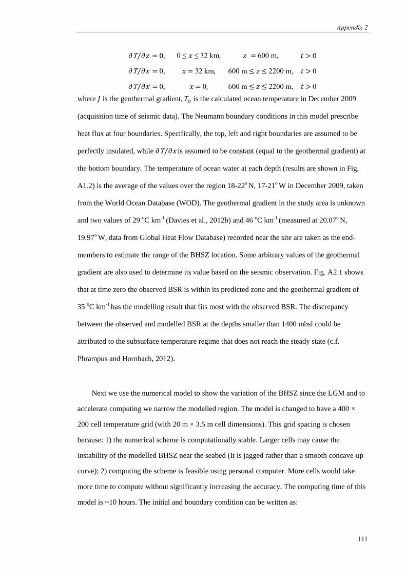
Appendix 2
111
∂T⁄∂z = 0, 0 ≤ 𝑥 ≤ 32 km, 𝑧 = 600 m, 𝑡 > 0
∂T⁄∂x = 0, 𝑥 = 32 km, 600 m ≤ 𝑧 ≤ 2200 m, 𝑡 > 0
∂T⁄∂x = 0, 𝑥 = 0, 600 m ≤ 𝑧 ≤ 2200 m, 𝑡 > 0
where 𝐽 is the geothermal gradient, 𝑇𝑜 is the calculated ocean temperature in December 2009
(acquisition time of seismic data). The Neumann boundary conditions in this model prescribe
heat flux at four boundaries. Specifically, the top, left and right boundaries are assumed to be
perfectly insulated, while ∂T⁄∂x is assumed to be constant (equal to the geothermal gradient) at
the bottom boundary. The temperature of ocean water at each depth (results are shown in Fig.
A1.2) is the average of the values over the region 18-22o N, 17-21
o W in December 2009, taken
from the World Ocean Database (WOD). The geothermal gradient in the study area is unknown
and two values of 29 oC km
-1 (Davies et al., 2012b) and 46
oC km
-1 (measured at 20.07
o N,
19.97o W, data from Global Heat Flow Database) recorded near the site are taken as the end-
members to estimate the range of the BHSZ location. Some arbitrary values of the geothermal
gradient are also used to determine its value based on the seismic observation. Fig. A2.1 shows
that at time zero the observed BSR is within its predicted zone and the geothermal gradient of
35 oC km
-1 has the modelling result that fits most with the observed BSR. The discrepancy
between the observed and modelled BSR at the depths smaller than 1400 mbsl could be
attributed to the subsurface temperature regime that does not reach the steady state (c.f.
Phrampus and Hornbach, 2012).
Next we use the numerical model to show the variation of the BHSZ since the LGM and to
accelerate computing we narrow the modelled region. The model is changed to have a 400 ×
200 cell temperature grid (with 20 m × 3.5 m cell dimensions). This grid spacing is chosen
because: 1) the numerical scheme is computationally stable. Larger cells may cause the
instability of the modelled BHSZ near the seabed (It is jagged rather than a smooth concave-up
curve); 2) computing the scheme is feasible using personal computer. More cells would take
more time to compute without significantly increasing the accuracy. The computing time of this
model is ~10 hours. The initial and boundary condition can be written as:

Appendix 2
112
T =𝑇𝑜′, 0 ≤ 𝑥 ≤ 8 km , 600 m ≤ 𝑧 ≤ 1300 m, 𝑡 = 0
∂T⁄∂z = J, 0 ≤ 𝑥 ≤ 8 km, 𝑧 = 1300 m, 𝑡 > 0
∂T⁄∂z = 0,
,
0 ≤ 𝑥 ≤ 8 km, 𝑧 = 600 m, 𝑡 > 0
∂T⁄∂x = 0, 𝑥 = 8 km, 600 m ≤ 𝑧 ≤ 1300 m 𝑡 > 0
∂T⁄∂x = 0, 𝑥 = 0, 600 m ≤ 𝑧 ≤ 1300 m 𝑡 > 0
where 𝑇𝑜′ is the initial temperature at 20 kyr ago. The bathymetry is from Fig. 4.2a and assumed
to be unchanged since 20 kyr ago. The data of RSL in the past 20 kyr are acquired by linearly
interpolation from fig.1 by Siddall et al. (2003) (Fig. A2.2a). We use the temperature anomalies
in Bintanja and van de Wal (2008) to estimate the variation of the temperature of deep ocean
with time (Fig. A2.2b). The effect on the deep-ocean temperature, which is from ice-sheet and
precipitating snow, is calculated through linear relation between the deep-water and the 3-kyr
mean surface air temperature anomalies based on a climate-ocean model (Bintanja and van
deWal, 2008). Heat transfer and time during hydrate formation and dissociation are not
considered. At each time step the reference frame of the vertical shift of the BHSZ is the seabed.
Eq. A2.1 is discretised in space using finite differences and then solved using the MATLAB
ordinary differential equation (ODE) solver, ODE45. The ODE45 solver is designed to solve the
ordinary differential equation and has an adaptive time stepping routine. The solver repeats its
calculations with successively smaller time-steps until the error between two results, generated
using Runge-Kutta 4th and Runge-Kutta 5th methods, is below a pre-defined error tolerance.
The solver is able to compute solutions much faster than conventional first-order explicit time-
stepping schemes without compromising accuracy.
Fig. A2.2c shows the BHSZ shoaled since the LGM at the site where the water depth is 825
m (its location is marked by the red triangle in Fig. 4.5). However, there are uncertainties in the
modelling and some of them stem from the input values of parameters. Results based on
different data show different degrees of oceanic warming, such as the data from the
Paleoclimate Modelling Intercomparision Project Phase 3 (PMIP3, the data can be downloaded
from https://pcmdi.llnl.gov/projects/esgf-llnl/) indicating that the temperature at the water depth
of 600 – 900 m have increased by 0.8 – 3.9 oC since 20 kyr ago. The data of BWT and RSL are

Appendix 2
113
not directly measured offshore of Mauritainia and may not suffice to reveal what happened in
the sutdy area.
Fig.A2.1 The modelled locations of the BHSZ with inputs of different geothermal gradient on a seismic
cross section. Their correlation with the observed BSR determines the geothermal gradient. The inset is
the temperature-depth plot of the ocean water.
Fig.A2.2 The variation of relative sea level (RSL) (a) and bottom water temperature (BWT) (b) in the last
20 kyr. The modelled variation of the BHSZ depth is shown in Fig. c. The site is marked by the red
triangle in Fig. 4.5. A gas chimney is observed here. mbsf – metres below seafloor.
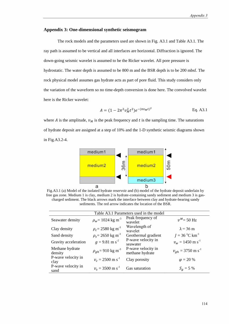
Appendix 3
114
Appendix 3: One-dimensional synthetic seismogram
The rock models and the parameters used are shown in Fig. A3.1 and Table A3.1. The
ray path is assumed to be vertical and all interfaces are horizontal. Diffraction is ignored. The
down-going seismic wavelet is assumed to be the Ricker wavelet. All pore pressure is
hydrostatic. The water depth is assumed to be 800 m and the BSR depth is to be 200 mbsf. The
rock physical model assumes gas hydrate acts as part of pore fluid. This study considers only
the variation of the waveform so no time-depth conversion is done here. The convolved wavelet
here is the Ricker wavelet:
𝐴 = (1 − 2𝜋2𝑣𝑀2 𝑡2)𝑒−(𝜋𝑣𝑀𝑡)2
Eq. A3.1
where 𝐴 is the amplitude, 𝑣𝑀 is the peak frequency and 𝑡 is the sampling time. The saturations
of hydrate deposit are assigned at a step of 10% and the 1-D synthetic seismic diagrams shown
in Fig.A3.2-4.
Fig.A3.1 (a) Model of the isolated hydrate reservoir and (b) model of the hydrate deposit underlain by
free gas zone. Medium 1 is clay, medium 2 is hydrate-containing sandy sediment and medium 3 is gas-
charged sediment. The black arrows mark the interface between clay and hydrate-bearing sandy
sediments. The red arrow indicates the location of the BSR.
Table A3.1 Parameters used in the model
Seawater density 𝜌𝑤= 1024 kg m-3
Peak frequency of wavelet 𝑣𝑀= 50 Hz
Clay density 𝜌𝑐= 2580 kg m-3 Wavelength of
wavelet λ = 36 m
Sand density 𝜌𝑠= 2650 kg m-3 Geothermal gradient 𝐽 = 36
oC km
-1
Gravity acceleration 𝑔 = 9.81 m s-2 P-wave velocity in
seawater 𝑣𝑤 = 1450 m s
-1
Methane hydrate density
𝜌𝑔ℎ= 910 kg m-3 P-wave velocity in
methane hydrate 𝑣𝑔ℎ = 3750 m s
-1
P-wave velocity in clay
𝑣𝑐 = 2500 m s-1
Clay porosity 𝜑 = 20 %
P-wave velocity in sand
𝑣𝑠 = 3500 m s-1 Gas saturation 𝑆𝑔 = 5 %

Appendix 3
115
Fig.A3.2 Synthetic seismic diagram of model a. Porosities of hydrate reservoir and clay are 30% and
20%. HC – hydrate concentration, RC – reflection coefficient for this and subsequent figures.
Fig.A3.3 Synthetic seismic diagram of model a. Porosities of hydrate reservoir and clay are 40% and
20%.
Fig.A3.4 Synthetic seismic diagram for the interface between hydrate-containing and gas-charged
sediments (model b).

Appendix 4
116
Appendix 4: Horizon maps
Block C-6
Fig.A4.1.A – dip magnitude map of seabed; B – RMS amplitude map of BSR; C – RMS amplitude map
of top of shear zone; D – RMS amplitude map of base of shear zone; E – RMS amplitude map of
reflection FGZ1; F – RMS amplitude map of reflection FGZ2; G – RMS amplitude map of reflection
FGZ3

Appendix 4
117
Fig
. A
4.2
A r
epre
sen
tati
ve
seis
mic
cro
ss s
ecti
on
of
blo
ck C
-6.
Its
loca
tio
n i
s sh
ow
n i
n F
ig.A
4.1
.Ple
ase
no
te t
he
ver
tica
l ex
agg
erat
ion
of
the
inse
t o
f th
e g
as c
him
ney
is
1.

Appendix 4
118
Block C-19
Fig.A4.3 A – dip magnitude map of seabed; B – RMS amplitude map of seabed; C – RMS amplitude map
of BSR; D – RMS amplitude map of reflection D. Reflections of A, B, C, E and F are stated in chapter 4.
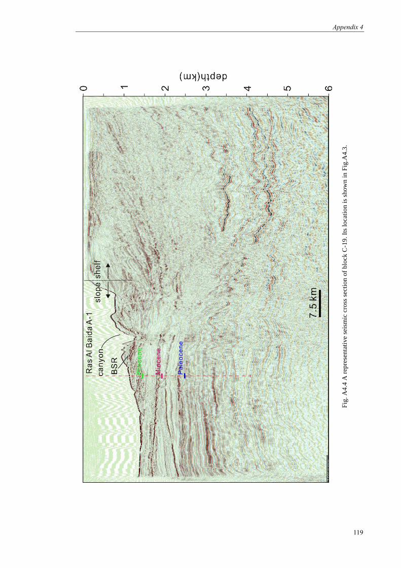
Appendix 4
119
Fig
. A
4.4
A r
epre
sen
tati
ve
seis
mic
cro
ss s
ecti
on
of
blo
ck C
-19
. It
s lo
cati
on i
s sh
ow
n i
n F
ig.A
4.3
.
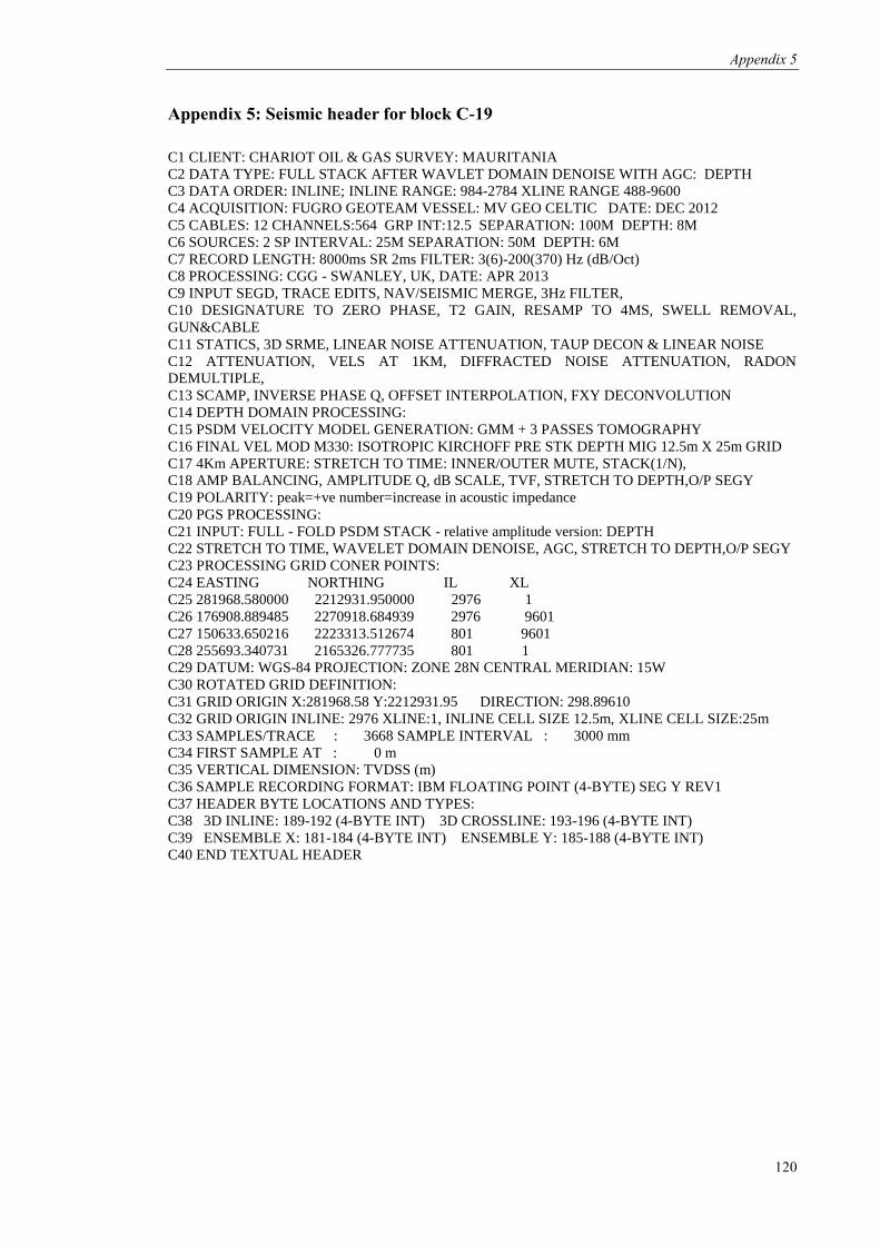
Appendix 5
120
Appendix 5: Seismic header for block C-19
C1 CLIENT: CHARIOT OIL & GAS SURVEY: MAURITANIA
C2 DATA TYPE: FULL STACK AFTER WAVLET DOMAIN DENOISE WITH AGC: DEPTH
C3 DATA ORDER: INLINE; INLINE RANGE: 984-2784 XLINE RANGE 488-9600
C4 ACQUISITION: FUGRO GEOTEAM VESSEL: MV GEO CELTIC DATE: DEC 2012
C5 CABLES: 12 CHANNELS:564 GRP INT:12.5 SEPARATION: 100M DEPTH: 8M
C6 SOURCES: 2 SP INTERVAL: 25M SEPARATION: 50M DEPTH: 6M
C7 RECORD LENGTH: 8000ms SR 2ms FILTER: 3(6)-200(370) Hz (dB/Oct)
C8 PROCESSING: CGG - SWANLEY, UK, DATE: APR 2013
C9 INPUT SEGD, TRACE EDITS, NAV/SEISMIC MERGE, 3Hz FILTER,
C10 DESIGNATURE TO ZERO PHASE, T2 GAIN, RESAMP TO 4MS, SWELL REMOVAL,
GUN&CABLE
C11 STATICS, 3D SRME, LINEAR NOISE ATTENUATION, TAUP DECON & LINEAR NOISE
C12 ATTENUATION, VELS AT 1KM, DIFFRACTED NOISE ATTENUATION, RADON
DEMULTIPLE,
C13 SCAMP, INVERSE PHASE Q, OFFSET INTERPOLATION, FXY DECONVOLUTION
C14 DEPTH DOMAIN PROCESSING:
C15 PSDM VELOCITY MODEL GENERATION: GMM + 3 PASSES TOMOGRAPHY
C16 FINAL VEL MOD M330: ISOTROPIC KIRCHOFF PRE STK DEPTH MIG 12.5m X 25m GRID
C17 4Km APERTURE: STRETCH TO TIME: INNER/OUTER MUTE, STACK(1/N),
C18 AMP BALANCING, AMPLITUDE Q, dB SCALE, TVF, STRETCH TO DEPTH,O/P SEGY
C19 POLARITY: peak=+ve number=increase in acoustic impedance
C20 PGS PROCESSING:
C21 INPUT: FULL - FOLD PSDM STACK - relative amplitude version: DEPTH
C22 STRETCH TO TIME, WAVELET DOMAIN DENOISE, AGC, STRETCH TO DEPTH,O/P SEGY
C23 PROCESSING GRID CONER POINTS:
C24 EASTING NORTHING IL XL
C25 281968.580000 2212931.950000 2976 1
C26 176908.889485 2270918.684939 2976 9601
C27 150633.650216 2223313.512674 801 9601
C28 255693.340731 2165326.777735 801 1
C29 DATUM: WGS-84 PROJECTION: ZONE 28N CENTRAL MERIDIAN: 15W
C30 ROTATED GRID DEFINITION:
C31 GRID ORIGIN X:281968.58 Y:2212931.95 DIRECTION: 298.89610
C32 GRID ORIGIN INLINE: 2976 XLINE:1, INLINE CELL SIZE 12.5m, XLINE CELL SIZE:25m
C33 SAMPLES/TRACE : 3668 SAMPLE INTERVAL : 3000 mm
C34 FIRST SAMPLE AT : 0 m
C35 VERTICAL DIMENSION: TVDSS (m)
C36 SAMPLE RECORDING FORMAT: IBM FLOATING POINT (4-BYTE) SEG Y REV1
C37 HEADER BYTE LOCATIONS AND TYPES:
C38 3D INLINE: 189-192 (4-BYTE INT) 3D CROSSLINE: 193-196 (4-BYTE INT)
C39 ENSEMBLE X: 181-184 (4-BYTE INT) ENSEMBLE Y: 185-188 (4-BYTE INT)
C40 END TEXTUAL HEADER


