Dymola Thermo-Bond-Graph Library - University of Arizonacellier/ece449_ppt22.pdf · The Dymola...

1

November 5, 2003Start Presentation

The Dymola Thermo-Bond-Graph Library• In this lecture, we shall introduce a second bond-graph

library, one designed explicitly to deal with convective flows.

• To this end, we shall need to introduce a new type of bonds, bonds carrying in parallel three distinct, yet inseparable, power flows: a heat flow, a volume flow, and a mass flow.

• These new bus-bonds, together with their corresponding bus-0-junctions, enable the modeler to describe convective flows at a high abstraction level.

• The example of a pressure cooker model completes the presentation.


Table of Contents• Thermo-bond graph connectors• A-causal and causal bonds• Bus-junctions• Heat exchanger• Volume work• Forced volume flow• Resistive field• Pressure cooker• Capacitive fields

• Evaporation and condensation• Simulation of pressure cooker• Free convective mass flow• Free convective volume flow• Forced convective volume flow• Water serpentine• Biosphere II

2


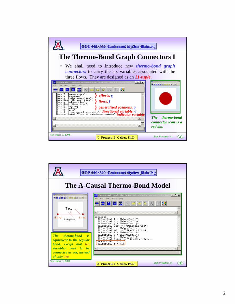
The Thermo-Bond Graph Connectors I• We shall need to introduce new thermo-bond graph

connectors to carry the six variables associated with the three flows. They are designed as an 11-tuple.

}}

efforts, eflows, f

} generalized positions, qdirectional variable, d

indicator variableThe thermo-bond connector icon is a red dot.


The A-Causal Thermo-Bond Model

d = −1 d = +1

The thermo-bond is equivalent to the regular bond, except that tenvariables need to be connected across, instead of only two.

3


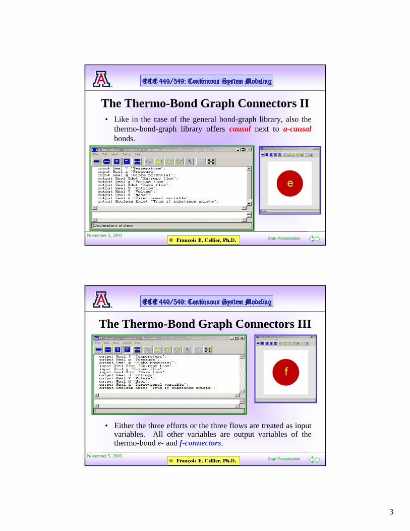
The Thermo-Bond Graph Connectors II• Like in the case of the general bond-graph library, also the

thermo-bond-graph library offers causal next to a-causalbonds.


The Thermo-Bond Graph Connectors III

• Either the three efforts or the three flows are treated as inputvariables. All other variables are output variables of the thermo-bond e- and f-connectors.

4


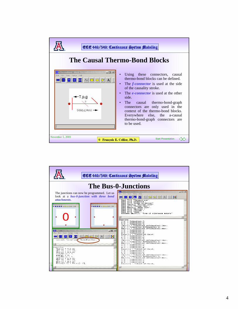
The Causal Thermo-Bond Blocks

• Using these connectors, causal thermo-bond blocks can be defined.

• The f-connector is used at the side of the causality stroke.

• The e-connector is used at the other side.

• The causal thermo-bond-graph connectors are only used in the context of the thermo-bond blocks. Everywhere else, the a-causal thermo-bond-graph connectors are to be used.


The Bus-0-JunctionsThe junctions can now be programmed. Let us look at a bus-0-junction with three bond attachments.

5


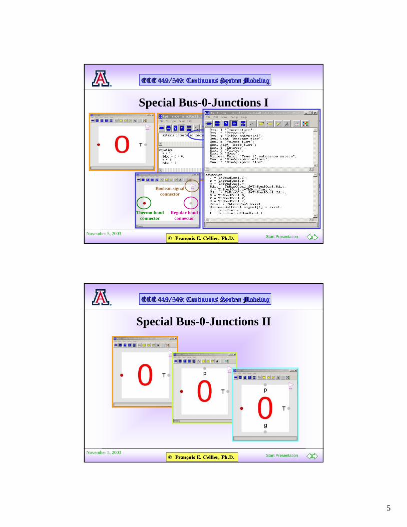
Special Bus-0-Junctions I

Thermo-bond connector

Regular bond connector

Boolean signal connector


Special Bus-0-Junctions II

6


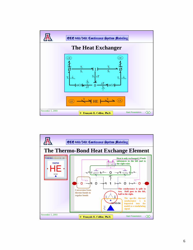
The Heat Exchanger

CFCF CFCF

11

∆T∆

2TS.

T

1

1

1 S.

1

S.

1

2

0 mGSmGS

2T

Ø Ø

∆T∆T S

.1

2

S.

12

S.

1x S.

2xT1 ∆

3 3

CFCF1CFCF2

3 3HE


The Thermo-Bond Heat Exchange Element

Conversion from thermo-bonds to regular bonds

The specific thermal conductance λ is imported into the model as a modulating signal.

The conductance is split in two. Half goes to the left, half to the right.

Heat is only exchanged, if both substances to the left and to the right exist.

7


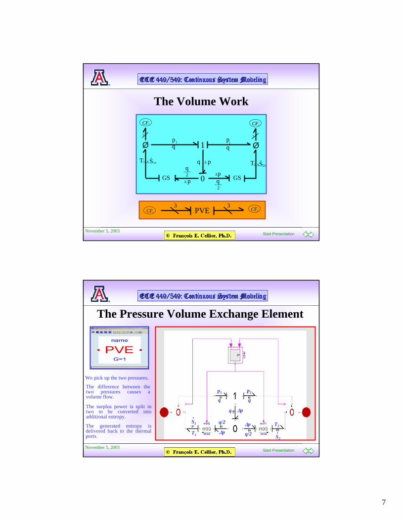
The Volume Work

pq q111 p

2

0 GSGS

2T1T

Ø Ø33

CFCF1 CFCF2

∆ pq

∆p∆ p

2q

2q

∆ S1x.

∆S2x.

CFCF1CFCF2

3 3PVE


The Pressure Volume Exchange Element

We pick up the two pressures.

p1 p2The difference between the two pressures causes a volume flow. q q

qThe surplus power is split in two to be converted into additional entropy.

∆p

∆p∆pq/2

q/2The generated entropy is delivered back to the thermal ports. T1

T2S1

.

S2

.

8


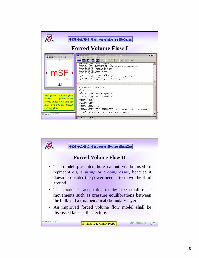
Forced Volume Flow I

The forced volume flow causes a proportional forced mass flow and an also proportional forced entropy flow.


Forced Volume Flow II

• The model presented here cannot yet be used to represent e.g. a pump or a compressor, because it doesn’t consider the power needed to move the fluid around.

• The model is acceptable to describe small mass movements such as pressure equilibrations between the bulk and a (mathematical) boundary layer.

• An improved forced volume flow model shall be discussed later in this lecture.

9


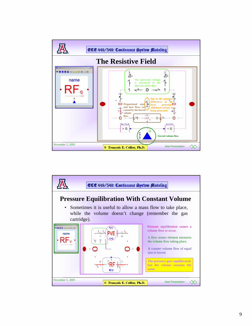
The Resistive Field

Forced volume flow

Proportional mass and heat flows are caused by the forced volume flow.

Due to the potential differences in the three potentials, additional entropy is being generated.

The generated entropy is reinserted in the direction of the flow.


Pressure Equilibration With Constant Volume• Sometimes it is useful to allow a mass flow to take place,

while the volume doesn’t change (remember the gas cartridge).

Pressure equilibration causes a volume flow to occur.

A flow sensor element measures the volume flow taking place.

A counter volume flow of equal size is forced.

The pressure gets equilibrated, but the volume remains the same.

10


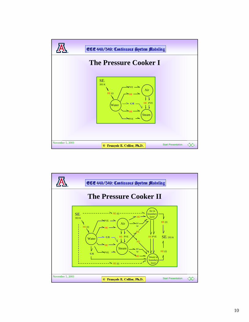
The Pressure Cooker I

Water

Air

Steam

SE: 393 K

HE (t)

C/E

PVE

PVE

HE

HE

HE PVE


The Pressure Cooker II

Water

Air

Steam

C/E

PVE

PVE

HE

HE

HE PVE

C/E

Air in boundary

layer

Steam in boundary

layer

HE

RF: ∆p

RF: ∆p

HE

HE PVE

HE

HE

SE: 293 K

HE (t)

HE (t)

SE: 393 K

HE (t)

HE (t)

HE (t)

11



Capacitive Fields• Let us look at the

capacitive field for air.

Linear capacitive field:der(e) = C · f

By integration:der(q) = fe = C · q

Non-linear capacitive field:der(q) = fe = e(q)

} der(q) = f

} e = e(q)The pressure is defined negative, in order to simplify dealing with the Gibbs equation.

12


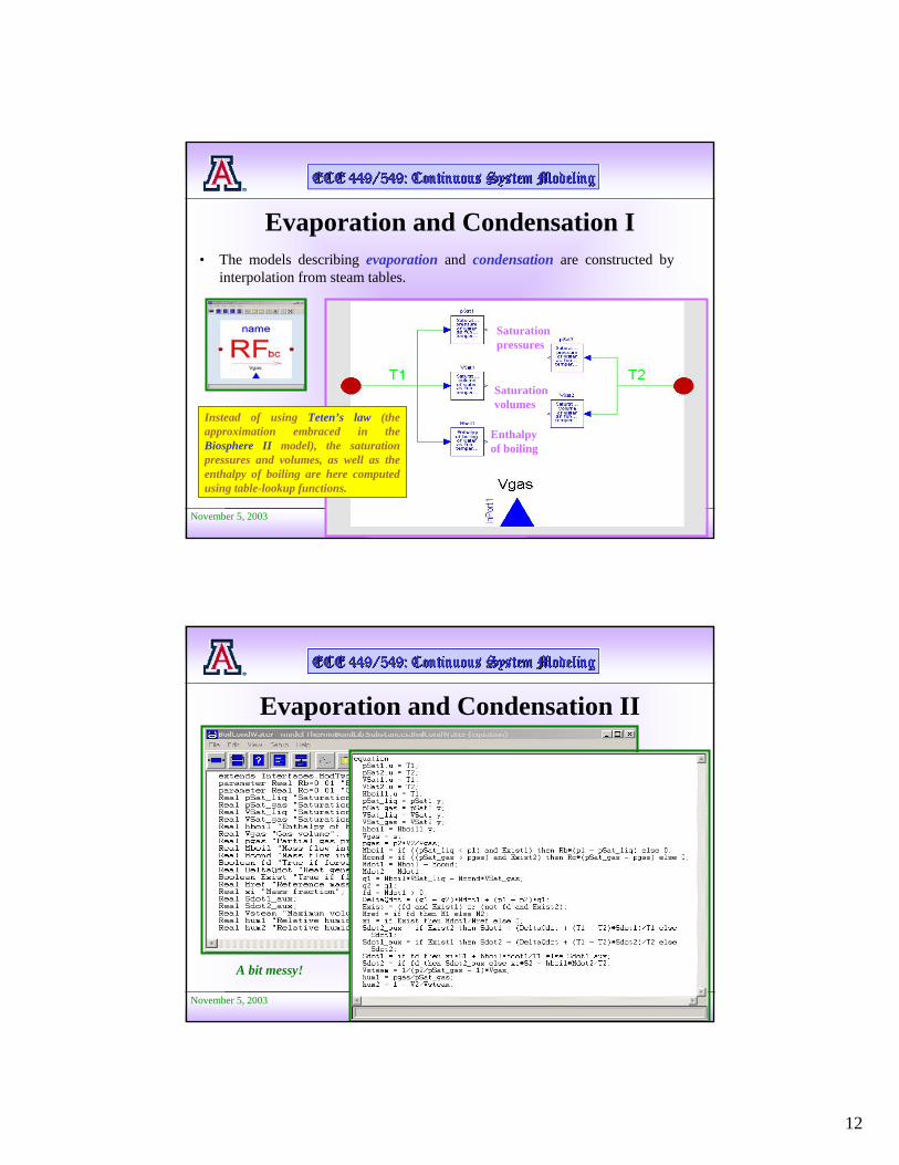
Evaporation and Condensation I• The models describing evaporation and condensation are constructed by

interpolation from steam tables.

Saturation pressures

Saturation volumes

Enthalpy of boiling

Instead of using Teten’s law (the approximation embraced in the Biosphere II model), the saturation pressures and volumes, as well as the enthalpy of boiling are here computed using table-lookup functions.


Evaporation and Condensation II

A bit messy!

13


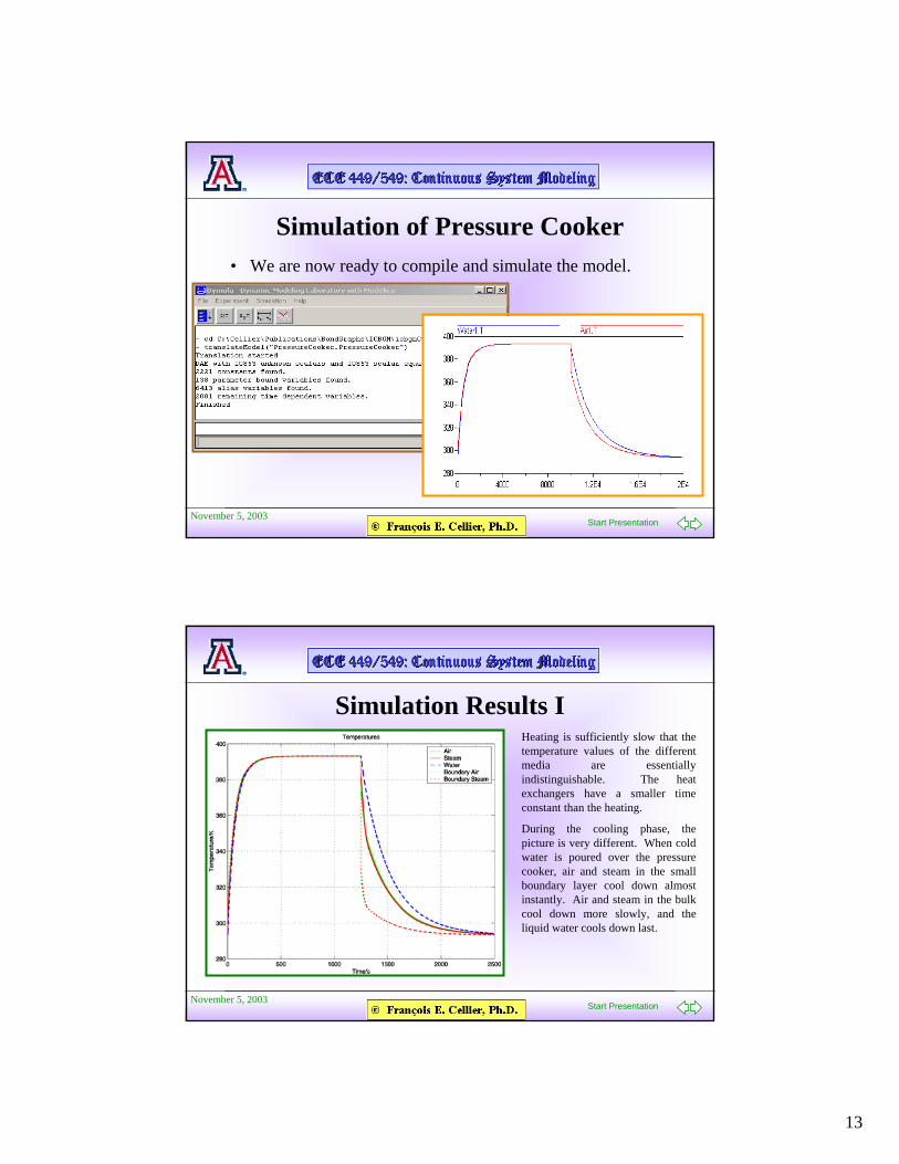
Simulation of Pressure Cooker• We are now ready to compile and simulate the model.


Simulation Results IHeating is sufficiently slow that the temperature values of the different media are essentially indistinguishable. The heat exchangers have a smaller time constant than the heating.

During the cooling phase, the picture is very different. When cold water is poured over the pressure cooker, air and steam in the small boundary layer cool down almost instantly. Air and steam in the bulk cool down more slowly, and the liquid water cools down last.

14


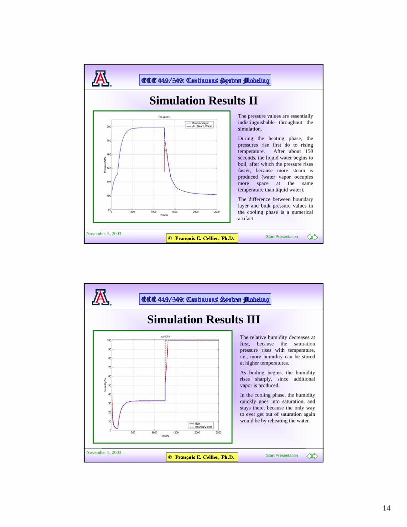
Simulation Results IIThe pressure values are essentially indistinguishable throughout the simulation.

During the heating phase, the pressures rise first do to rising temperature. After about 150 seconds, the liquid water begins to boil, after which the pressure rises faster, because more steam is produced (water vapor occupies more space at the same temperature than liquid water).

The difference between boundary layer and bulk pressure values in the cooling phase is a numerical artifact.


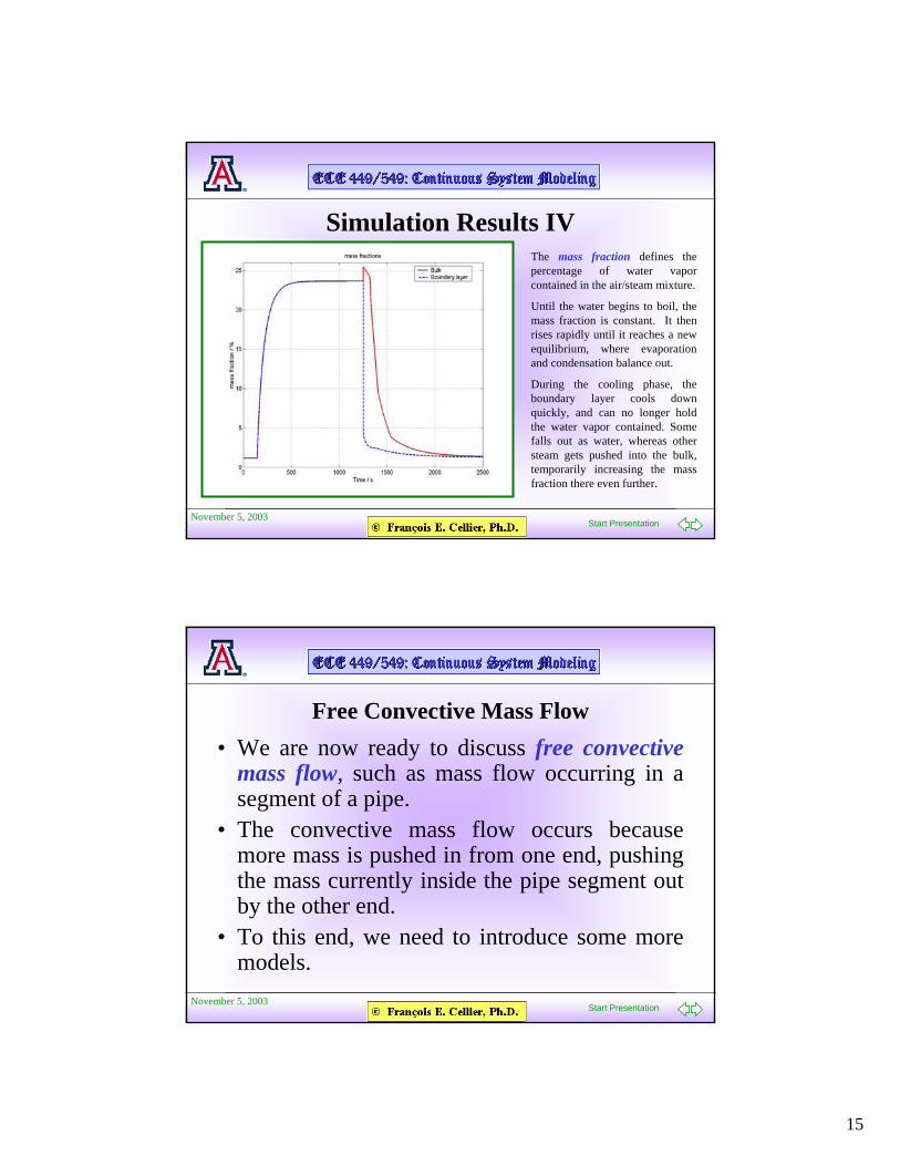
Simulation Results IIIThe relative humidity decreases at first, because the saturation pressure rises with temperature, i.e., more humidity can be stored at higher temperatures.

As boiling begins, the humidity rises sharply, since additional vapor is produced.

In the cooling phase, the humidity quickly goes into saturation, and stays there, because the only way to ever get out of saturation again would be by reheating the water.

15


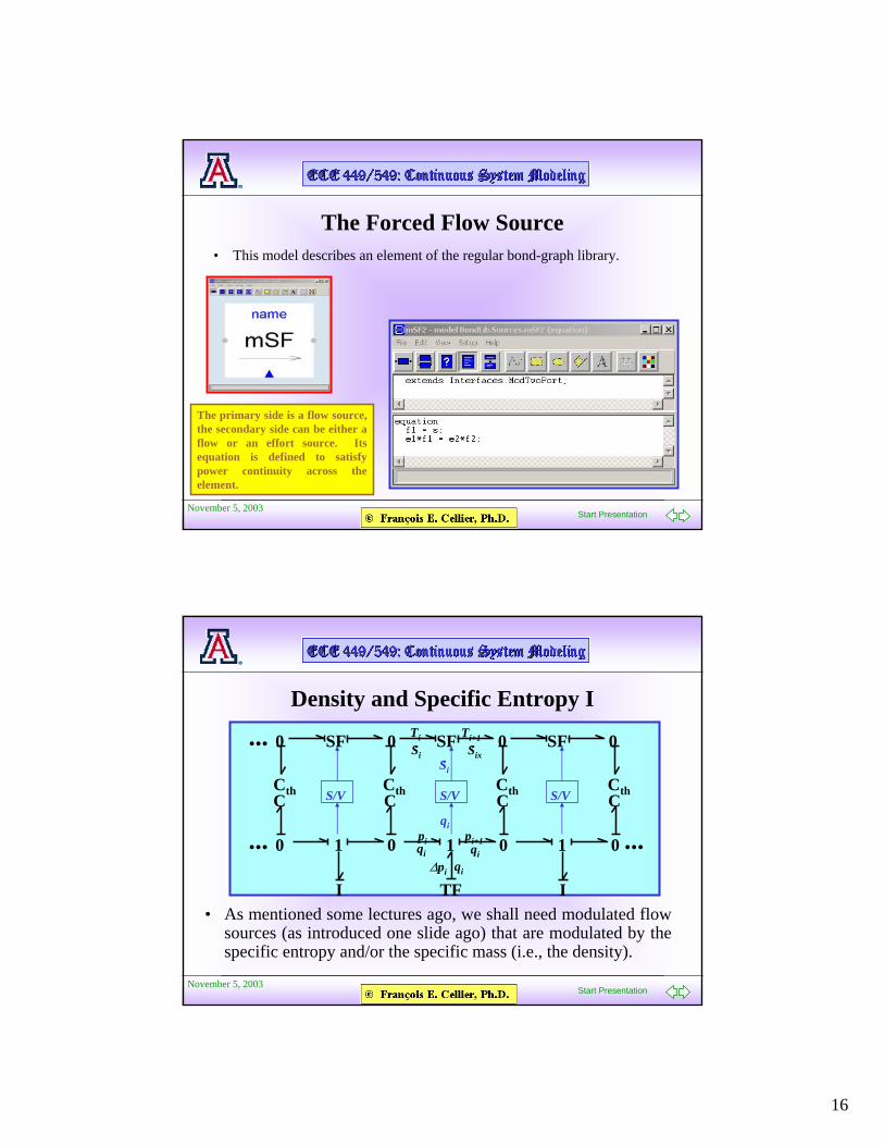
Simulation Results IVThe mass fraction defines the percentage of water vapor contained in the air/steam mixture.

Until the water begins to boil, the mass fraction is constant. It then rises rapidly until it reaches a new equilibrium, where evaporation and condensation balance out.

During the cooling phase, the boundary layer cools down quickly, and can no longer hold the water vapor contained. Some falls out as water, whereas other steam gets pushed into the bulk, temporarily increasing the mass fraction there even further.


Free Convective Mass Flow• We are now ready to discuss free convective

mass flow, such as mass flow occurring in a segment of a pipe.

• The convective mass flow occurs because more mass is pushed in from one end, pushing the mass currently inside the pipe segment out by the other end.

• To this end, we need to introduce some more models.

16


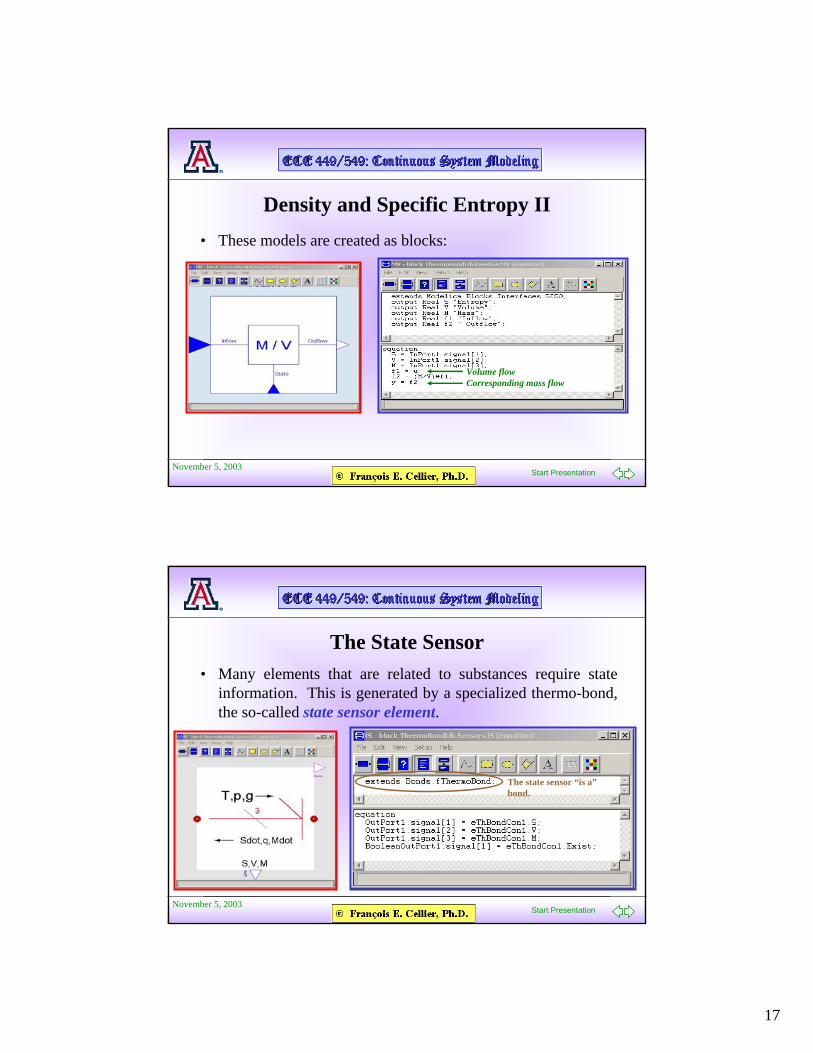
The Forced Flow Source• This model describes an element of the regular bond-graph library.

The primary side is a flow source, the secondary side can be either a flow or an effort source. Its equation is defined to satisfy power continuity across the element.


Density and Specific Entropy I

• As mentioned some lectures ago, we shall need modulated flow sources (as introduced one slide ago) that are modulated by the specific entropy and/or the specific mass (i.e., the density).

... 0 1 0 1 0 1 ...0

C

I

C C C

TF I

qi

pi pi+1

∆pi qi

qi

Cth

0... SF 0 SF 0 SF 0

Cth Cth CthS/V S/V S/V

qi

Si.Si

. Six.Ti Ti+1

17


Density and Specific Entropy II• These models are created as blocks:

Volume flowCorresponding mass flow


The State Sensor• Many elements that are related to substances require state

information. This is generated by a specialized thermo-bond, the so-called state sensor element.

The state sensor “is a” bond.

18


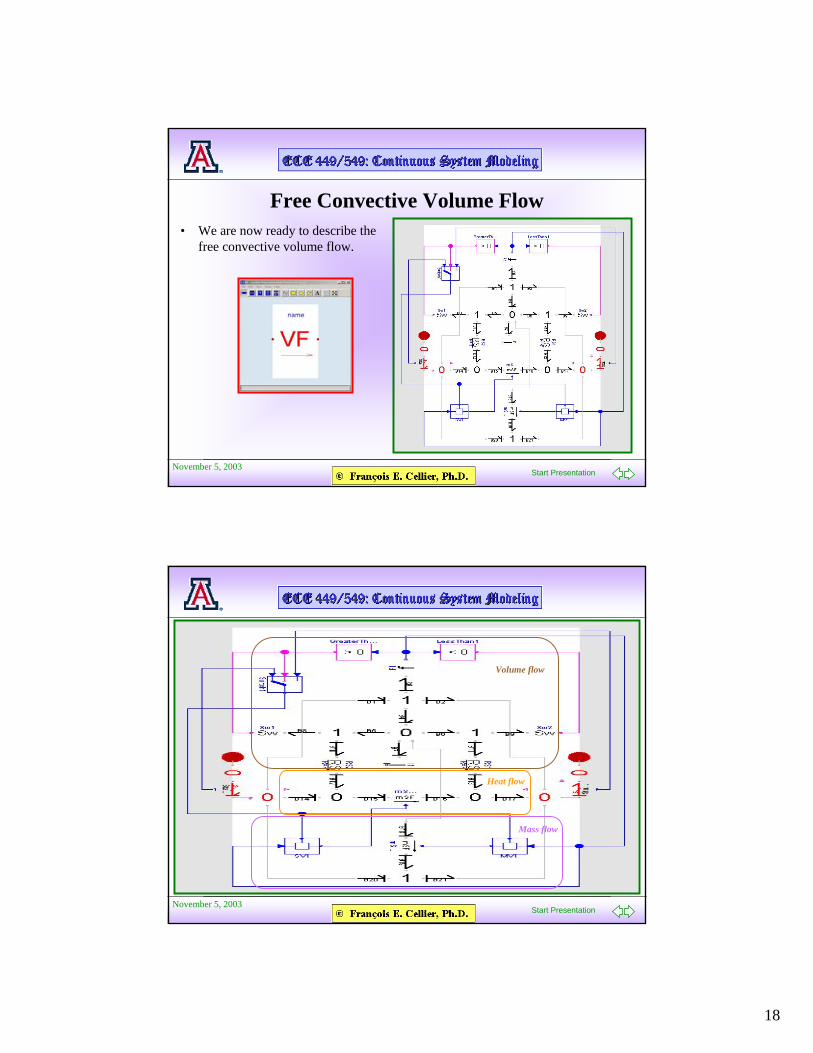
Free Convective Volume Flow• We are now ready to describe the

free convective volume flow.


Volume flow

Heat flow

Mass flow

19


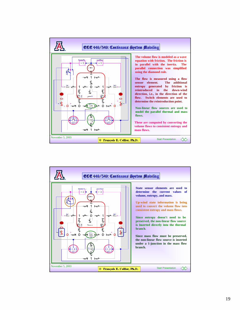
The volume flow is modeled as a wave equation with friction. The friction is in parallel with the inertia. The parallel connection was simplified using the diamond rule.

The flow is measured using a flow sensor element. The additional entropy generated by friction is reintroduced in the down-wind direction, i.e., in the direction of the flow. Switch elements are used to determine the reintroduction point.

Non-linear flow sources are used to model the parallel thermal and mass flows.

These are computed by converting the volume flows to consistent entropy and mass flows.


State sensor elements are used to determine the current values of volume, entropy, and mass.

Up-wind state information is being used to convert the volume flow into consistent entropy and mass flows.

Since entropy doesn’t need to be preserved, the non-linear flow source is inserted directly into the thermal branch.

Since mass flow must be preserved, the non-linear flow source is inserted under a 1-junction in the mass flow branch.

20


The Gibbs equation can be written as:

U = T · S - p · q + g · M· · ·

or more conveniently as:

U = Q - p · q + g · M· · ·

Thus, the change of the internal energy can be written as:

δU = δ Q - δ p · q + δ g · M· · ·

In a segment of pipe, both the heatand the internal energy are conserved, thus:

δU = δ Q = 0· ·

Hence: δ p · q = δ g · M·g1 g2

M.

M.

M. g2 – g1

p1 p2

p1 – p2

q qq

∆q

p1 – p2


Forced Convective Volume Flow• We are now ready to describe the

forced convective mass flow.

The model is almost the same as the free convective flow model, except that a volume flow is forced on the system through the regular bond connector at the top.

21


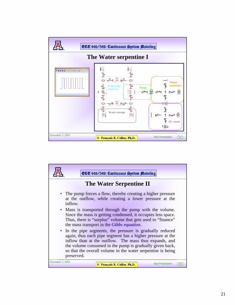
The Water serpentine I

DC-motor

Piston mechanics

PumpWater pipe segments

Water storage


The Water Serpentine II• The pump forces a flow, thereby creating a higher pressure

at the outflow, while creating a lower pressure at the inflow.

• Mass is transported through the pump with the volume. Since the mass is getting condensed, it occupies less space. Thus, there is “surplus” volume that gets used to “finance” the mass transport in the Gibbs equation.

• In the pipe segments, the pressure is gradually reduced again, thus each pipe segment has a higher pressure at the inflow than at the outflow. The mass thus expands, and the volume consumed in the pump is gradually given back, so that the overall volume in the water serpentine is being preserved.

22


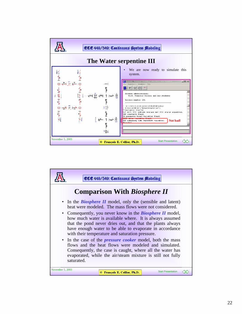
The Water serpentine III• We are now ready to simulate this

system.

Not bad!


Comparison With Biosphere II• In the Biosphere II model, only the (sensible and latent)

heat were modeled. The mass flows were not considered.• Consequently, you never know in the Biosphere II model,

how much water is available where. It is always assumed that the pond never dries out, and that the plants always have enough water to be able to evaporate in accordance with their temperature and saturation pressure.

• In the case of the pressure cooker model, both the mass flows and the heat flows were modeled and simulated. Consequently, the case is caught, where all the water has evaporated, while the air/steam mixture is still not fully saturated.

23


References I• Cellier, F.E. and J. Greifeneder (2003), “Object-oriented modeling of

convective flows using the Dymola thermo-bond-graph library,” Proc. ICBGM’03, Intl. Conference on Bond Graph Modeling and Simulation, Orlando, FL, pp. 198 – 204.

• Greifeneder, J. and F.E. Cellier (2001), “Modeling multi-element systems using bond graphs,” Proc. ESS’01, European Simulation Symposium, Marseille, France, pp. 758 – 766.

• Brück, D., H. Elmqvist, H. Olsson, and S.E. Mattsson (2002), “Dymola for Multi-Engineering Modeling and Simulation,” Proc. 2nd

International Modelica Conference, pp. 55:1-8.


References II

• Cellier, F.E. (2001), The Dymola Bond-Graph Library.

• Cellier, F.E. (2001), The Dymola Thermo-Bond-Graph Library.

• Cellier, F.E. (2002), The Dymola Pressure Cooker Model.

• Cellier, F.E. (2002), The Dymola Water Serpentine Model.

Date post:	12-Apr-2018
Category:	Documents
Upload:	dohuong
View:	219 times
Download:	2 times

Dymola Thermo-Bond-Graph Library - University of Arizonacellier/ece449_ppt22.pdf · The Dymola...

Documents