DYNAMIC AND STATIC WETTABILITY OF ADVANCED MATERIALS USED IN AERONAUTICAL APPLICATIONS
OMID GOHARDANI & DAVID W. HAMMONDDepartment of Power and Propulsion, Cranfi eld University, Bedford, UK.
ABSTRACTThe search for icephobic external surface materials in aircraft icing applications has been ongoing since the early days of aviation. Given the recognized superlative properties of carbon nanotubes (CNTs) across many different disciplines, the implementation of CNTs in polymer matrix composites has sparked a great interest in their mechanical/electrical properties and wetting character, in addition to their suitability for aircraft icing applications. Within this framework, a new developed methodology capable of determining the nature of wettability, consequent to CNT implementation is desired. Thus, this article presents a novel methodology – henceforth referred to as the dynamic and static wettability scheme for advanced materials – which examines the wettability of materials reinforced with CNTs, for potential utilization within the aerospace industry. The described methodology herein can be employed in order to numerically examine empirically acquired results with an extended possibility to include alternative materials outside the scope of the considered ones. Results are shown for a decision matrix that discriminates between hydrophobic and hydrophilic surfaces based on their static and dynamic wettability properties. Moreover, idealized wetting character representations of the different considered aerospace materials are presented.Keywords: aerospace materials, aircraft icing, carbon nanotube wettability, corona splashing measure-ment tool, dynamic and static wettability scheme for advanced materials, fl uid structures, hydrophilicity, hydrophobicity, liquid water concentration.
1 INTRODUCTIONThe usage of polymeric matrix composites has become more frequent in a number of different industries including electronics, the automotive and the aerospace industry [1]. The aerospace sector in particular has embraced the usage of polymeric matrix composites in civil and military aircraft, often with weight consideration in mind. Due to the superior mechanical and physical properties that have been observed in carbon nanotubes (CNTs), a natural consideration is whether CNTs can be utilized as reinforcing agents to further enhance the mechanical and physical properties of polymeric matrix composites. For this reason, researchers have con-ducted various research efforts in order to examine the infl uence of CNTs on the mechanical properties of the aforementioned materials [2,24]. A factor of great importance in aerospace applications due to high speed fl ight of, for instance, Earth entry vehicles and aircraft, is erosion [3]. In particular, Gohardani et al. [4], examined the erosion resilience, mechanical properties and acoustic impedance of a selection of polymer matrix composites reinforced with CNTs at 0.5% wt. for potential use in aeronautics. In this study, some disparities were observed between the different properties of the materials, but nominally similar erosion resilience values for the considered materials were encountered despite the presence of CNTs. The reasoning behind this observation was attributed to the dispersion process of CNTs in the resin. The infl u-ence of CNTs on the hydrophobic and hydrophilic nature of a set of specimens was further considered by Gohardani and Hammond [5] based on empirical results. Following the introduc-tion of novel propulsion cycles such as distributed technology [6,7] and their perspective applications [8], the present study describes a proposed methodology by Gohardani and Hammond [9] and exhibits numerical representations of the wettability of a number of CNT reinforced composites with potential usage within aeronautics.
O. Gohardani & D.W. Hammond, Int. J. Comp. Meth. and Exp. Meas., Vol. 1, No. 3 (2013) 299
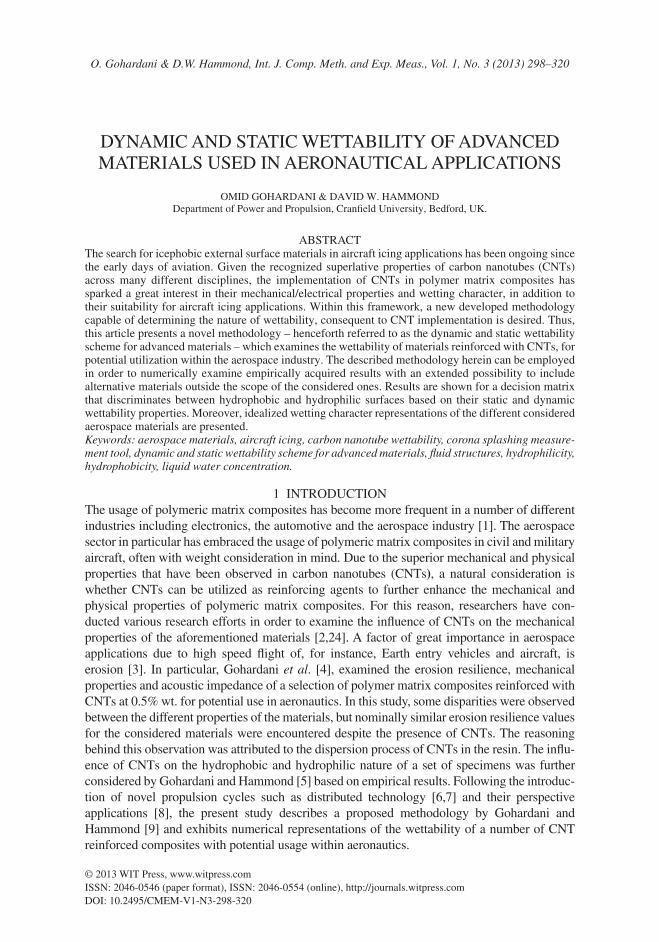
2 EXPERIMENTAL SETUPThe dynamic wettability experiments were carried out at the vertical droplet tunnel located at Cranfi eld University, United Kingdom. The fl ow was powered by a centrifugal backward curved suction fan, capable of producing fl ow rates, m. Fan ∈ [30,100] kg ⋅ s–1. The temperature range T ∈ [–30, +30] °C, was obtained by the air and refrigeration plant with a capacity of 400 kW, capable of extracting the heat from the air [10]. Wetting of a target specimen was attained by a droplet generator ejecting mono dispersed droplets at a frequency of fd ≈ 12 kHz, positioned at the entrance section of the droplet tunnel. Figure 1, shows a rendering of the experimental setup for the dynamic wettability experiments.
Two different illumination techniques were utilized in order to visualize the droplets and the wetting characteristics of the surface. The LED captured splashing features apparent in the volume of space along the width of each specimen, while the 2 mm laser sheet was employed in order to establish the local liquid water concentration. The image acquisition was actualized by employing a Sony XCD-SX90 camera operated at 30 FPS. The experimen-tal images were acquired upon utilizing a graphical user interface (GUI) on a personal computer.
2.1 Material substrates
A total number of 10 different materials referred to hereafter with a specimen number Sn were utilized in this study, in two different prescribed conditions; as supplied and in an eroded condition, with n = {1, 2, ..., 10}. The majority of these specimens were established epoxy resins commonly used within the aerospace industry with addition of CNTs as a reinforcing agent. Specimens S1 and S2 were both combinations of Araldite® LY564/Aradur® 2954 with the exception that specimen S2 also featured multi-walled CNTs (MWCNT) at 0.5% wt. Graphistrength® C100. Specimens S3, S4, S5 and S6 were Araldite® MY0510/Aradur® 976-1
Figure 1: The experimental setup for the dynamic wettability experiments with notations: (A) Vertical droplet tunnel, (B) droplet cloud, (C) charge-coupled device camera, (D) laser sheet, (E) laser, (F) control valves, (G) light-emitting diode (LED) strobing device, (H) collimating lens, and (I) specimen target. The right hand side image depicts a schematic corona structure with virtual planes i 0, . . . , i N , with im showing the mid-plane of the corona.
AB
I
E
HG
F
C
D
i 0im
iN
300 O. Gohardani & D.W. Hammond, Int. J. Comp. Meth. and Exp. Meas., Vol. 1, No. 3 (2013)
combinations, with S4 and S6 having 0.5% wt. MWCNT as a reinforcement. Specimen S7 was an Araldite® DBF/Aradur® HY956EN base resin with 10% wt. aluminum nitride nanoparti-cles, and specimen S8 a gelcoat consisting of a SW404/XB5173 combination. Adopting this nomenclature classifi ed specimens S2, S4 and S6 as reinforced with CNTs. The materials were examined both in their pristine state and upon a wet blasting process which resulted in an averaged degraded surface fi nish Re
a ≅ 4 mm, implying a higher surface roughness in relation to the averaged surface roughness value in the pristine state.
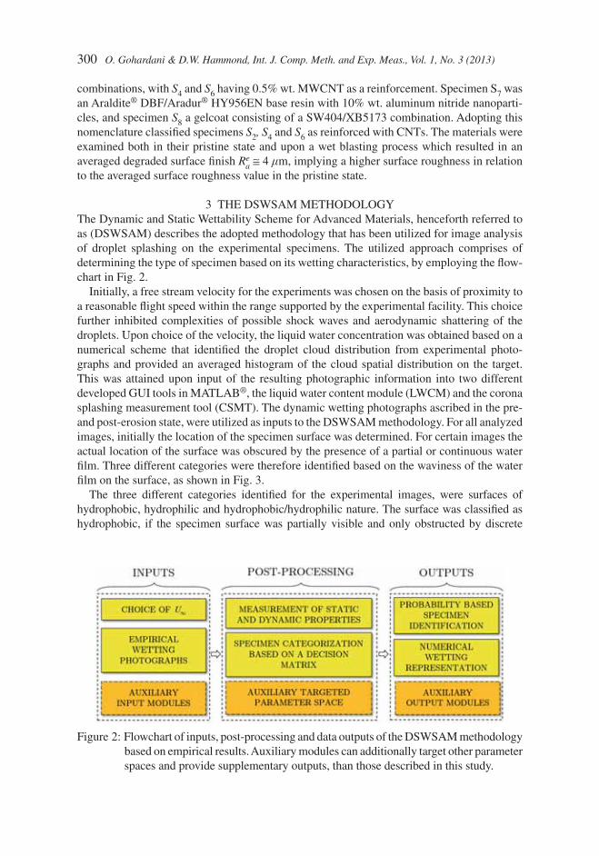
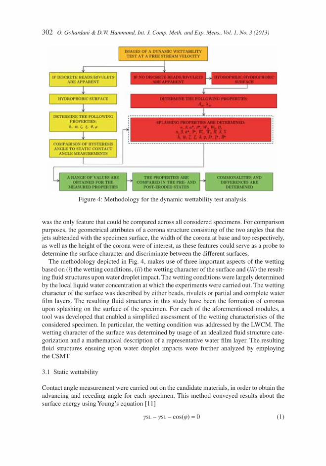
3 THE DSWSAM METHODOLOGYThe Dynamic and Static Wettability Scheme for Advanced Materials, henceforth referred to as (DSWSAM) describes the adopted methodology that has been utilized for image analysis of droplet splashing on the experimental specimens. The utilized approach comprises of determining the type of specimen based on its wetting characteristics, by employing the fl ow-chart in Fig. 2.
Initially, a free stream velocity for the experiments was chosen on the basis of proximity to a reasonable fl ight speed within the range supported by the experimental facility. This choice further inhibited complexities of possible shock waves and aerodynamic shattering of the droplets. Upon choice of the velocity, the liquid water concentration was obtained based on a numerical scheme that identifi ed the droplet cloud distribution from experimental photo-graphs and provided an averaged histogram of the cloud spatial distribution on the target. This was attained upon input of the resulting photographic information into two different developed GUI tools in MATLAB®, the liquid water content module (LWCM) and the corona splashing measurement tool (CSMT). The dynamic wetting photographs ascribed in the pre- and post-erosion state, were utilized as inputs to the DSWSAM methodology. For all analyzed images, initially the location of the specimen surface was determined. For certain images the actual location of the surface was obscured by the presence of a partial or continuous water fi lm. Three different categories were therefore identifi ed based on the waviness of the water fi lm on the surface, as shown in Fig. 3.
The three different categories identifi ed for the experimental images, were surfaces of hydrophobic, hydrophilic and hydrophobic/hydrophilic nature. The surface was classifi ed as hydrophobic, if the specimen surface was partially visible and only obstructed by discrete
Figure 2: Flowchart of inputs, post-processing and data outputs of the DSWSAM methodology based on empirical results. Auxiliary modules can additionally target other parameter spaces and provide supplementary outputs, than those described in this study.
O. Gohardani & D.W. Hammond, Int. J. Comp. Meth. and Exp. Meas., Vol. 1, No. 3 (2013) 301
ligaments of water, as shown in Figs. 3 (a) and (b). If a continuous water fi lm layer was present on the specimen surface, it was categorized as a hydrophilic surface, as shown in Figs. 3 (c) and (d). For instances where an intermediate water fi lm layer with partial characteristics of a continuous water fi lm was identifi ed, the specimen was either classifi ed as hydrophilic or hydrophobic, visualized in Figs. 3 (e) and (f). For hydrophobic surfaces based on Figs. 3 (a) and (b) and the corresponding description, the number of fl uid ligaments along the surface of the specimen were counted. A larger number of ligaments in this respect represented a more hydrophobic surface. For a hydrophilic surface, Figs. 3 (c) and (d), and a surface where the hydrophobic or hydrophilic surface character was diffi cult to categorize, as shown in Figs. 3 (e) and (f), the averaged wave lengths of the structures were determined. As the interaction of droplets on the specimen surface with and without an existing wetting character during the experiments largely resulted in formation of coronas, the structure of a water splash corona
Figure 3: Idealized hydrophobic and hydrophilic wetting structures on different specimen surfaces with corresponding representative experimental photographs. Examples of hydrophobic surfaces are shown in (a) and (b). Figures (c) and (d) show a hydrophilic surface. Figures (e) and (f) fi nally represent a hydrophobic/hydrophilic surface.
302 O. Gohardani & D.W. Hammond, Int. J. Comp. Meth. and Exp. Meas., Vol. 1, No. 3 (2013)
was the only feature that could be compared across all considered specimens. For comparison purposes, the geometrical attributes of a corona structure consisting of the two angles that the jets subtended with the specimen surface, the width of the corona at base and top respectively, as well as the height of the corona were of interest, as these features could serve as a probe to determine the surface character and discriminate between the different surfaces.
The methodology depicted in Fig. 4, makes use of three important aspects of the wetting based on (i) the wetting conditions, (ii) the wetting character of the surface and (iii) the result-ing fl uid structures upon water droplet impact. The wetting conditions were largely determined by the local liquid water concentration at which the experiments were carried out. The wetting character of the surface was described by either beads, rivulets or partial and complete water fi lm layers. The resulting fl uid structures in this study have been the formation of coronas upon splashing on the surface of the specimen. For each of the aforementioned modules, a tool was developed that enabled a simplifi ed assessment of the wetting characteristics of the considered specimen. In particular, the wetting condition was addressed by the LWCM. The wetting character of the surface was determined by usage of an idealized fl uid structure cate-gorization and a mathematical description of a representative water fi lm layer. The resulting fl uid structures ensuing upon water droplet impacts were further analyzed by employing the CSMT.
3.1 Static wettability
Contact angle measurement were carried out on the candidate materials, in order to obtain the advancing and receding angle for each specimen. This method conveyed results about the surface energy using Young’s equation [11]
gSL – gSL – cos(j) = 0 (1)
Figure 4: Methodology for the dynamic wettability test analysis.
O. Gohardani & D.W. Hammond, Int. J. Comp. Meth. and Exp. Meas., Vol. 1, No. 3 (2013) 303
where g is the energy and the subscripts SG and SL denote solid-gas and solid-liquid respectively. The drop was modifi ed by either dispensing or retracting its volume, resulting in an advancing angle qA or a receding angle qR, measured by a protractor. This method allowed for an assessment of the homogeneity of the specimen, as droplets could be depos-ited on various locations on the specimen surface. In this study an averaged value of fi ve measurements placed on different locations on the surface is presented. Hysteresis y, can in this context be defi ned as y = qA–qR. The equilibrium Young contact angle qC can further be expressed in terms of the advancing and receding angles [12] as
q
q qC
A A R R
A R
=++
⎧⎨⎩
⎫⎬⎭
arccoscos( ) cos( )Γ Γ
Γ Γ (2)
where
Γ A R
A R
A R A R,
,
, ,
/sin ( )
cos( ) cos ( )=
− +
⎧⎨⎪
⎩⎪
⎫⎬⎪
⎭⎪
3
3
1 3
2 3
q
q q (3)
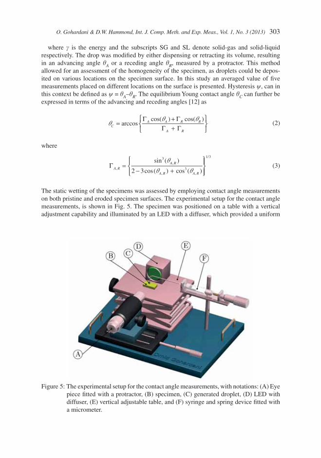
The static wetting of the specimens was assessed by employing contact angle measurements on both pristine and eroded specimen surfaces. The experimental setup for the contact angle measurements, is shown in Fig. 5. The specimen was positioned on a table with a vertical adjustment capability and illuminated by an LED with a diffuser, which provided a uniform
Figure 5: The experimental setup for the contact angle measurements, with notations: (A) Eye piece fi tted with a protractor, (B) specimen, (C) generated droplet, (D) LED with diffuser, (E) vertical adjustable table, and (F) syringe and spring device fi tted with a micrometer.
304 O. Gohardani & D.W. Hammond, Int. J. Comp. Meth. and Exp. Meas., Vol. 1, No. 3 (2013)
illumination of the droplet. The 5 cc syringe with a glass luer slip tip, fi tted with a 6″ needle and 90° blunt end, produced the 2.04 mm drop of deionized water. The volume of fl uid utilized for these measurements ranged between 10–90 ml. The uncertainty of the measure-ments was mainly related to the manual goniometry readings of the back-lit droplet’s advancing and receding angles. Since imperfections in surface uniformity and cleanness could be present at the time of the readings, an error of ~ 5° was expected for the contact angle measurements. The setup utilized for measurement of the advancing and receding contact angles on S1–S10 is shown in Fig. 5.
3.2 Wetting condition
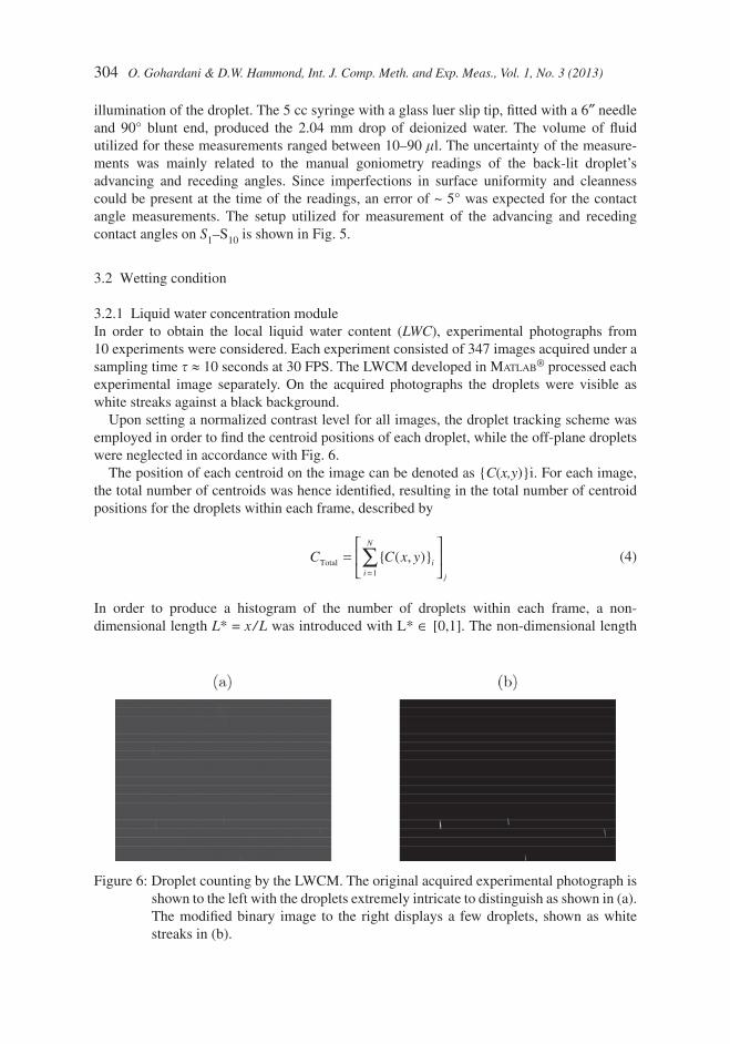
3.2.1 Liquid water concentration moduleIn order to obtain the local liquid water content (LWC), experimental photographs from 10 experiments were considered. Each experiment consisted of 347 images acquired under a sampling time t ≈ 10 seconds at 30 FPS. The LWCM developed in MATLAB® processed each experimental image separately. On the acquired photographs the droplets were visible as white streaks against a black background.
Upon setting a normalized contrast level for all images, the droplet tracking scheme was employed in order to fi nd the centroid positions of each droplet, while the off-plane droplets were neglected in accordance with Fig. 6.
The position of each centroid on the image can be denoted as {C(x,y)}i. For each image, the total number of centroids was hence identifi ed, resulting in the total number of centroid positions for the droplets within each frame, described by
C C x y i
i
N
j
Total =⎡
⎣⎢
⎤
⎦⎥
=∑{ ( , )}
1
(4)
In order to produce a histogram of the number of droplets within each frame, a non- dimensional length L* = x / L was introduced with L* ∈ [0,1]. The non-dimensional length
Figure 6: Droplet counting by the LWCM. The original acquired experimental photograph is shown to the left with the droplets extremely intricate to distinguish as shown in (a). The modifi ed binary image to the right displays a few droplets, shown as white streaks in (b).
O. Gohardani & D.W. Hammond, Int. J. Comp. Meth. and Exp. Meas., Vol. 1, No. 3 (2013) 305
along the specimen was further divided into 10 equally sized bins. The allocation of each centroid position i, to each bin k, was actualized by
nLC L
n Li
*( *)
( ) *
10
1
10≤ <
+ (5)
with n = 0, 1, ..., 9, i = 1, 2, ..., N and k = 1, 2, ..., 10.For each centroid position fulfi lling eqn (5), an increment was added to the total number of
droplets within each bin mk. The total number of droplets for a given frame was hence given by
N mj k
k
N
==
∑1
(6)
The averaged number of droplets within a sequence of images, in a given zone, were further given by
R
nDj i
i
n
j
=⎧⎨⎪
⎩⎪
⎫⎬⎪
⎭⎪=∑1
1 (7)
where i = {1, 2, ..., n}, j = {1, 2, ..., 10} and n is the number of frames equal to 347. With known number of droplets, a similar approach for estimation of the local Liquid Water Con-tent (LWC) as Ide [13] was employed. For a constant droplet diameter, D and total sample area for the bins Ã, the LWC can be expressed as
LWC
D
AU tRj
i
≅∞
∑rp 3
6 % (8)
where r is the water density, t is the sampling time, U• is the free stream velocity, and the sum refers to the total number of droplets.
3.3 Wetting character of the surface
In order to adopt a nomenclature that could easily be measured empirically and identifi ed analytically, a number of different structures describing possible wetting features of the surfaces were defi ned, as shown in Fig. 7.
Four fl uid structure classifi cations, Categories I–IV were identifi ed within the population, to be present on the specimen surface, upon impact of the droplet stream onto the surface, within the fi eld of view of the camera. The parameters shown in Fig. 7 refer to the measured parameters and the output column to results produced by this module. Categories I and II, represent idealized bead and rivulet structures, respectively. As fl uid structures of each pre-sented category in Fig. 7, feature different geometrical sizes, a representative fl uid structure for each category was determined upon averaging over a large population of images, with the considered structures.
The distinction between a bead (Category I) and a rivulet (Category II) was largely deter-mined by x >> w, for a rivulet, while h ~ z. The distinction criterion employed herein was that a structure was categorized as a rivulet if x > l / 2, where l is the length of the specimen within the fi eld of view. This criterion, clearly distinguished between beads and rivulets as a more moderate length restriction on x would make the distinction more diffi cult. Due to the larger spatial extent of a rivulet, it can be stated that the number of beads in general was greater than
306 O. Gohardani & D.W. Hammond, Int. J. Comp. Meth. and Exp. Meas., Vol. 1, No. 3 (2013)
the number of rivulets, nb > nr. A large population of beads on the surface nb >> 1, further inferred that the surface was hydrophobic.
A continuous water fi lm (Category III) was present in the case where x → ∞, with the amplitude of each wave Ai > 0. A partial water fi lm was further apparent when Ai > 0 was followed by Ai + 1 → 0 and Ai + 2 > 0, along the entire surface of the specimen, in a continuous manner. Hence, it could readily be established that Category II differed from Category III, as it had a more discrete character.
The ensuing fl uid structure following the impact of an incoming droplet of size d, was a corona structure, shown in Category IV. The employed nomenclature hence determined the corona structure parameters regardless of the initial formed surface fl uid classifi cation (Categories I–III). A set of parameters that addressed a comparison between the incoming and splashing structure were hence, h* ≡ H / (h + d), z* ≡ H / (z + d) and A* ≡ H / (d + A). The reasoning behind analyzing the geometrical parameters of the corona structures across all considered specimens was to provide a metric for wettability of each material. In particular this method was useful, upon analyzing the wetting character of the pre- and post eroded specimens, as it provided an insight into the infl uence of erosion on the wetting character of each specimen.
The defi ned structures in Fig. 7, were idealized for simplicity and described merely by the shown geometrical properties. Although shape deviations from the idealized structures existed in comparison to the encountered structures during the experimental runs, the defi ned geometrical structures at large, adequately captured the behavior of the fl uid characters on the surface and allowed for simple measurements of the fl uid features by utilizing a personal computer.
Figure 7: Fluid structure categories with corresponding measured parameters and outputs upon employing the DSWSAM methodology.
O. Gohardani & D.W. Hammond, Int. J. Comp. Meth. and Exp. Meas., Vol. 1, No. 3 (2013) 307
In order to analyze the experimental photographs, a baseline for the location of the top sur-face of the specimen was established by utilizing the ImageJ software. All categories except Category IV were thereafter discretized by positioning of nodes ni = {1, 2, ..., N}, using the multi-point tool in ImageJ. The intermediate distance between the points, Ωi = |xi+1 − xi| hence represented different length scales where Ωi = li denoted the wavelength of the water fi lm, Ωi = wi width of a bead and Ωi = xi width of a rivulet, depending on the analyzed struc-tures. The height of each structure Ξi = |yapex – yi| was defi ned as the distance between the base and the apex of the structure, with Ξi = Ai denoting the amplitude of the water fi lm, Ξi = hi representing the height of a bead and Ξi = zi identifying the height of a rivulet. A surface cov-ered with beads could in an idealized representation consist of n number of beads, each having a width wn and height hn placed adjacent to each other, described by
B x
h x xH H w
wnn n n n
n
( )( )
=− + − +4 8 42 2 2 1
2
(9)
where the horizontal distance of each bead’s apex position from the origin Hn was defi ned as
H x
n
w n
H w w nn
w
w
n n n
( )
,
,
,
≡
=
+ =+ + >
⎧
⎨⎪⎪
⎩⎪⎪ − −
1
2
2
1 2
1 1
1
2
2
(10)
A representative bead structure could further be expressed as
B x
h x w
w( )
( )=
− +4 2 2
(11)
with h = ΣNn = 1 hi / n and w = ΣN
n = 1 wi / n determined from the experiments. The idealized water fi lm layer could similarly be expressed by
W x A x B( ) sin( )= +w % (12)
where B% is a constant, w = 2p / |l| and the parameters A = ΣNn = 1 Ai / n and l = ΣN
n = 1 li / n were determined upon discretization using the empirical photographs. The water fi lm layer was then confi ned between the function W(x) and y = 0, for x ∈ [0, ∞).
Upon visual representation of the results, it is often useful to express the parameters in non-dimensional form in order to facilitate the comparison between different surfaces regard-less of the length of the specimen. The used notation herein is based on the total length of the specimen in the fi eld of view l, upon empirical image acquisition. For a bead, the non- dimensional height and width were given by h* = h / l and w* = w / l. The number of beads was further enumerated by nst and the number of spacings between the beads given by nsp. These notations hence implied that nst > nsp.
The event where nst >> nsp was evident, upon a cluster of beads being encountered on the surface and placed adjacent to each other. Similarly for a rivulet, the height and width were denoted by z* = z / l and x* = x / l. For rivulets, the number of spacings were not considered, allowing the plurality of rivulets to be represented by a single rivulet with the mean value of height and width established by the considered rivulets. Lastly for a water fi lm A* = A / l, denoted the non-dimensional amplitude and l* = l / l, the non-dimensional wavelength of the water fi lm. In the idealized representations of the surface structures, shown in Figs. 11 and 12, only the number of bead structures nst was considered.
308 O. Gohardani & D.W. Hammond, Int. J. Comp. Meth. and Exp. Meas., Vol. 1, No. 3 (2013)
3.4 Resulting fl uid structures upon impact
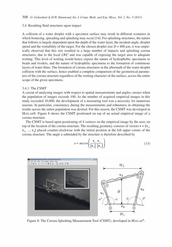
A collision of a water droplet with a specimen surface may result in different scenarios in which bouncing, spreading and splashing may occur [14]. For splashing structures, the nature that follows is largely dependent upon the depth of the water layer, the incident angle, droplet speed and the wettability of the target. For the chosen droplet size D = 400 mm, it was empir-ically observed that this size resulted in a large number of impacts and splashing corona structures, due to the local LWC and was capable of exposing the target area to adequate wetting. This level of wetting would hence expose the nature of hydrophobic specimens to beads and rivulets, and the nature of hydrophilic specimens to the formation of continuous layers of water fi lms. The formation of corona structures in the aftermath of the water droplet collision with the surface, hence enabled a complete comparison of the geometrical parame-ters of the corona structure regardless of the wetting character of the surface, across the entire scope of the given specimens.
3.4.1 The CSMTA caveat of analyzing images with respect to spatial measurements and angles, ensues when the population of images exceeds 100. As the number of acquired empirical images in this study exceeded 16,000, the development of a measuring tool was a necessity for numerous reasons. In particular, consistency during the measurements and robustness in obtaining the results across the entire population was desired. For this reason, the CSMT was developed in MATLAB®. Figure 8 shows the CSMT positioned on top of an actual empirical image of a corona structure.
The CSMT is based upon positioning of 4 vertices on the empirical image by the user, on top of the location of the corona structure. The resulting geometry consists of vectors v = {v1, v2, ..., v4} placed counter-clockwise with the initial position at the left upper corner of the corona structure. The angle a subtended by the structure is therefore described by
a =
⋅⋅
⎛
⎝⎜⎞
⎠⎟arccos
v v
v v1 2
1 2
(13)
Figure 8: The Corona Splashing Measurement Tool (CSMT), developed in MATLAB®.
O. Gohardani & D.W. Hammond, Int. J. Comp. Meth. and Exp. Meas., Vol. 1, No. 3 (2013) 309
Similarly the angle b is given by
b =⋅⋅( )
⎛
⎝⎜
⎞
⎠⎟arccos
v v
v v2 3
2 3
(14)
In addition, the angles fulfi ll the requirement of a + a* = 180° and b + b* = 180°. The height of the corona H, is with the given nomenclature described by
H =−( )
h
2 4 2v v (15)
where
h = −( ) −( ) − −( ) − −( )4 2 4 4 3 4 1s s s sv v v v v v (16)
and s is given by
s =
+ + +v v v v1 2 3 4
2 (17)
The two-dimensional area of the corona structure is hence given by
A
H≈
⋅ +( )v v2 4
2 (18)
In order to estimate the amount of variability in pixel intensity within the region of interest subtended by the 4 vertices of the corona structure, the entropy within the region of the exper-imental photographs was computed. The entropy for a grayscale image in MATLAB®, is defi ned as a measure of the randomness associated with the texture of the image [15], and is com-puted according to
%E p p= − ⋅∑ log ( )2 (19)
where p contains the count of the histogram. This approach is applied both to the entropy of the entire image resulting in the entropy of the frame, EF and confi ned only to the corona for which EC is computed. This parameter provides an insight into the uniformity of the pixel intensity within the corona structure, as recorded on the experimental photograph. Smooth textures hence result in lower and rough textures in higher entropy values. The CMST pro-duces measurements of the corona structure given by the generic function
Φ = f W W H E EC F( , , *, *, , , , , , )a b a b 1 2 A (20)
The CSMT outputs the parameters given in eqn (20) for a given initial position of the vertices designated by pi(xi, yi) with i = 1 ... 4, implying in an output from the generic function Φp. If the position of any of the i:th coordinates is altered resulting in p′i(x′i; y′i) with i = 1 ... 4, and p ≠ p′, the software is capable of producing a new generic function Φp¢. The repositioning procedure can hence be carried out until the vertices of the CSMT are superimposed on top of the four edges of the corona structure on the empirical image. This results in a fi nal generic function for the specifi c frame ΦF, with F ∈ [0, N], where N is a positive integer. Based on the measured parameters, a range of non-dimensional factors were obtained for the splashing
310 O. Gohardani & D.W. Hammond, Int. J. Comp. Meth. and Exp. Meas., Vol. 1, No. 3 (2013)
structures. These properties were measured both in the pre- and post eroded states of the specimens, respectively and their commonalities and differences were determined. Four dif-ferent combination of geometrical parameters were considered in order to establish the behavior of the corona structure. The initial one examined the skewness of the corona by determining the ratio a* / b*. In this respect, three different cases could unfold according to:
a
b
*
*=
− >=
− <
Right skewed corona
Neutral corona
left skewed corona
1
1
11
⎧⎨⎪
⎩⎪ (21)
The second parameter of interest was (W2 – W1) / W1, which described the expansion of base width, to the top width of the corona, in percent. A value of (W2 – W1) / W 1 > 1, hence implied an expansion and (W2 – W1) / W1 < 1, a reduction of width in comparison to the base width of the corona. The aspect ratio of the corona was furthermore given by (W1 + W2) / 2H . A value of (W1 + W2) / 2H = 1, was indicative of a square shaped corona, and (W1 + W2) / 2H > 1, a rectangular shaped corona structure.
3.5 The infl uence of the boundary layer
In order to estimate the infl uence of the boundary layer on the incoming droplets, a simpli-fi ed approach can be considered for estimation of the size of the boundary layer thickness. Under the assumption that the stagnation point is located suffi ciently far away from the leading edge of the specimen, the fl ow over the specimen surface can be approximated as the fl ow over a fl at plate with an incident angle a = 0°. For a fi nite length of the plate x, the inertial force r ru u x U x∂ ∂( ) ( )∞/ ~ / .2 The friction force per unit volume is however given by dt / dy ~ (mU∞) / d2. Equating the inertial and friction forces yields d(x) ~ {(mx) / (rU∞)}
12 . If
the position of the boundary layer thickness is determined when u = 0.99U∞, the boundary layer thickness can be defi ned as [16]
d99 5 0≈
∞
.vx
U (22)
The reduction of volume fl ux due to the action of viscosity or the displacement thickness d1 and other parameters such as the momentum thickness d2 and the energy thickness d3, are further given by eqns (23)–(25)
d1
0
1= −⎛⎝⎜
⎞⎠⎟∞
∞
∫u
Udy (23)
d2
0
1= −⎛⎝⎜
⎞⎠⎟∞
∞
∞∫
u
U
u
Udy (24)
d3
0
2
21= −
⎛
⎝⎜
⎞
⎠⎟
∞
∞
∫∞
u
U
u
Udy
(25)
Moreover, the wall shear stress is approximated by tw (x) ≈ {(rmU3∞) / x}
12 and the skin-friction
coeffi cient by cf (x) ≈ 2tw(x) / (rU∞)2. The splashing phenomenon is often related to different non-dimensional parameters such as the Reynolds number based on the diameter Red = (rU∞d) / m, the Weber number Wed = (rU2
∞d) / s, the Ohnsorge number Oh We= /Re, and the
O. Gohardani & D.W. Hammond, Int. J. Comp. Meth. and Exp. Meas., Vol. 1, No. 3 (2013) 311
Capillary number Ca = We / Re, where d is the droplet diameter, r defi nes the density, U∞ is the free stream velocity, m is the dynamic viscosity, and s denotes the surface tension. The spreading factor %x = /d d,max can further be expressed as [17]
%x
q
=+
− +⎛⎝⎜
⎞⎠⎟
We
WeA
12
3 14
cos( )Re
(26)
4 RESULTS AND DISCUSSIONTable 1, shows the advancing, receding, equilibrium Young contact angle and their corre-sponding hysteresis.
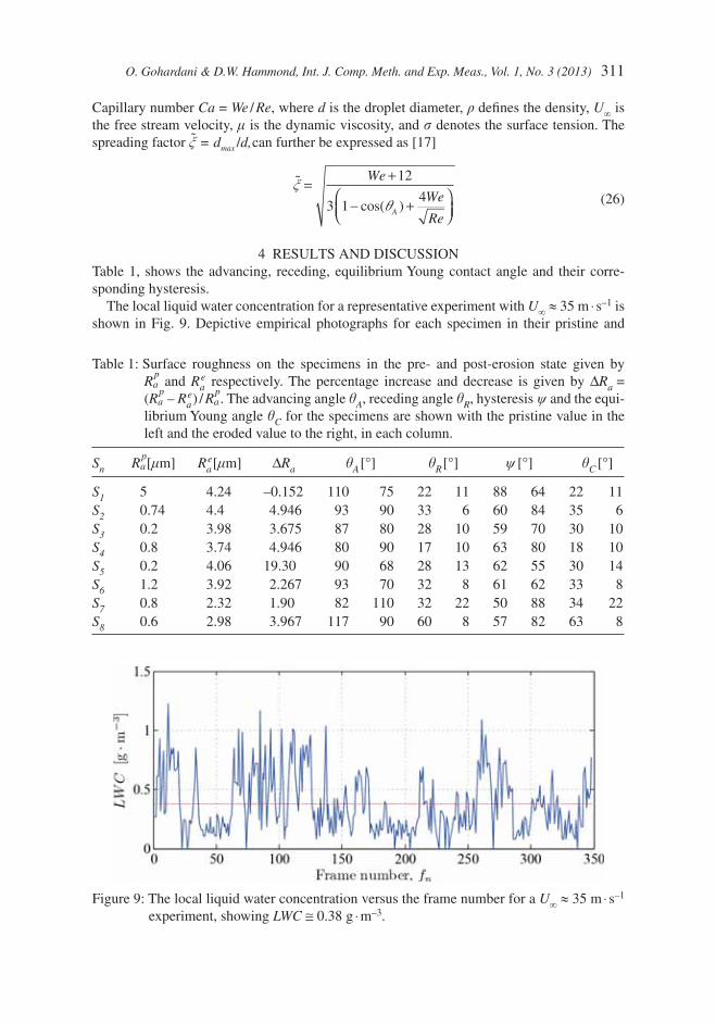
The local liquid water concentration for a representative experiment with U∞ ≈ 35 m ⋅ s–1 is shown in Fig. 9. Depictive empirical photographs for each specimen in their pristine and
Table 1: Surface roughness on the specimens in the pre- and post-erosion state given by R
pa and Re
a respectively. The percentage increase and decrease is given by ΔRa = (R
pa – Re
a) / Rpa . The advancing angle qA, receding angle qR, hysteresis y and the equi-
librium Young angle qC for the specimens are shown with the pristine value in the left and the eroded value to the right, in each column.
Figure 9: The local liquid water concentration versus the frame number for a U∞ ≈ 35 m ⋅ s–1 experiment, showing LWC ≅ 0.38 g ⋅ m–3.
312 O. Gohardani & D.W. Hammond, Int. J. Comp. Meth. and Exp. Meas., Vol. 1, No. 3 (2013)
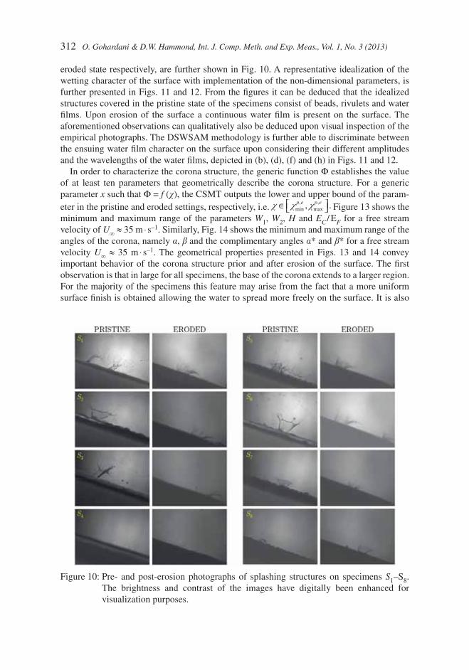
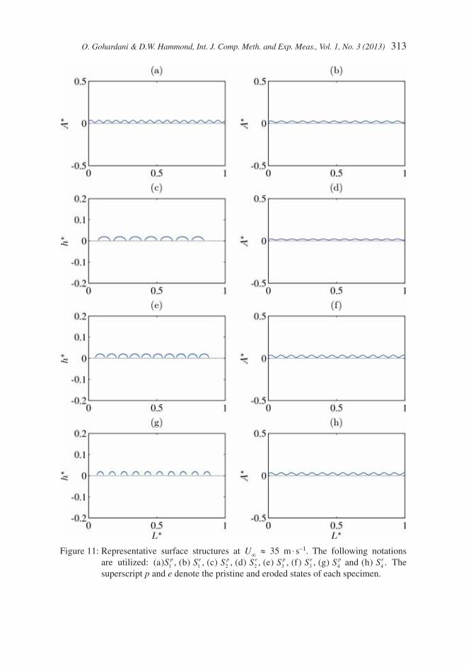
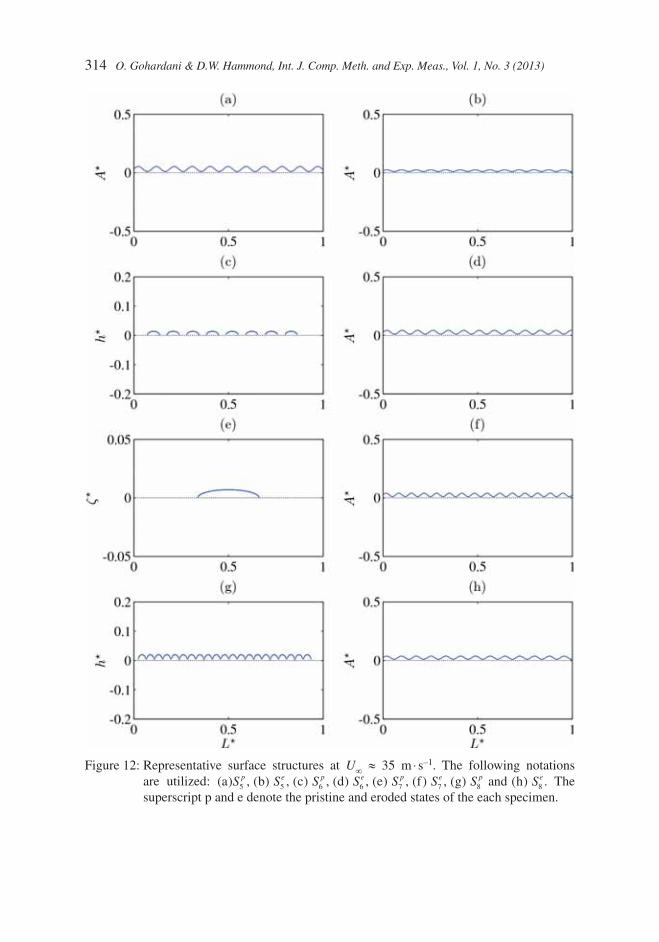
eroded state respectively, are further shown in Fig. 10. A representative idealization of the wetting character of the surface with implementation of the non-dimensional parameters, is further presented in Figs. 11 and 12. From the fi gures it can be deduced that the idealized structures covered in the pristine state of the specimens consist of beads, rivulets and water fi lms. Upon erosion of the surface a continuous water fi lm is present on the surface. The aforementioned observations can qualitatively also be deduced upon visual inspection of the empirical photographs. The DSWSAM methodology is further able to discriminate between the ensuing water fi lm character on the surface upon considering their different amplitudes and the wavelengths of the water fi lms, depicted in (b), (d), (f) and (h) in Figs. 11 and 12.
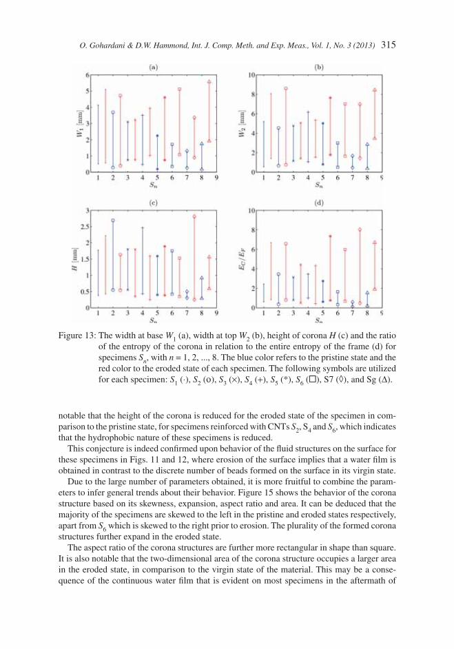
In order to characterize the corona structure, the generic function Φ establishes the value of at least ten parameters that geometrically describe the corona structure. For a generic parameter x such that Φ = f (c), the CSMT outputs the lower and upper bound of the param-eter in the pristine and eroded settings, respectively, i.e. c c c∈⎡⎣ ⎤⎦min
,max
,, .p e p e Figure 13 shows the
minimum and maximum range of the parameters W1, W2, H and EC / EF for a free stream velocity of U∞ ≈ 35 m ⋅ s–1. Similarly, Fig. 14 shows the minimum and maximum range of the angles of the corona, namely a, b and the complimentary angles a* and b* for a free stream velocity U∞ ≈ 35 m ⋅ s–1. The geometrical properties presented in Figs. 13 and 14 convey important behavior of the corona structure prior and after erosion of the surface. The fi rst observation is that in large for all specimens, the base of the corona extends to a larger region. For the majority of the specimens this feature may arise from the fact that a more uniform surface fi nish is obtained allowing the water to spread more freely on the surface. It is also
Figure 10: Pre- and post-erosion photographs of splashing structures on specimens S1–S8. The brightness and contrast of the images have digitally been enhanced for visualization purposes.
O. Gohardani & D.W. Hammond, Int. J. Comp. Meth. and Exp. Meas., Vol. 1, No. 3 (2013) 313
Figure 11: Representative surface structures at U∞ ≈ 35 m ⋅ s–1. The following notations are utilized: ( ) , ( ) , ( ) , ( ) , ( ) , ( ) , ( ) ( ) .a b c d e f g and hS S S S S S S Sp e p e p e p e
1 1 2 2 3 3 4 4 The superscript p and e denote the pristine and eroded states of each specimen.
314 O. Gohardani & D.W. Hammond, Int. J. Comp. Meth. and Exp. Meas., Vol. 1, No. 3 (2013)
Figure 12: Representative surface structures at U∞ ≈ 35 m ⋅ s–1. The following notations are utilized: ( ) , ( ) , ( ) , ( ) , ( ) , ( ) , ( ) ( ) .a b c d e f g and hS S S S S S S Sp e p e p e p e
5 5 6 6 7 7 8 8 The superscript p and e denote the pristine and eroded states of the each specimen.
O. Gohardani & D.W. Hammond, Int. J. Comp. Meth. and Exp. Meas., Vol. 1, No. 3 (2013) 315
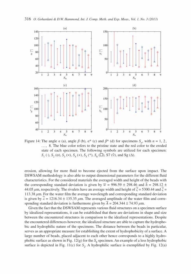
Figure 13: The width at base W1 (a), width at top W2 (b), height of corona H (c) and the ratio of the entropy of the corona in relation to the entire entropy of the frame (d) for specimens Sn, with n = 1, 2, ..., 8. The blue color refers to the pristine state and the red color to the eroded state of each specimen. The following symbols are utilized for each specimen: S1 (⋅), S2 (ο), S3 (×), S4 (+), S5 (*), S6 ( ), S7 (◊), and Sg (Δ).
notable that the height of the corona is reduced for the eroded state of the specimen in com-parison to the pristine state, for specimens reinforced with CNTs S2, S4 and S6, which indicates that the hydrophobic nature of these specimens is reduced.
This conjecture is indeed confi rmed upon behavior of the fl uid structures on the surface for these specimens in Figs. 11 and 12, where erosion of the surface implies that a water fi lm is obtained in contrast to the discrete number of beads formed on the surface in its virgin state.
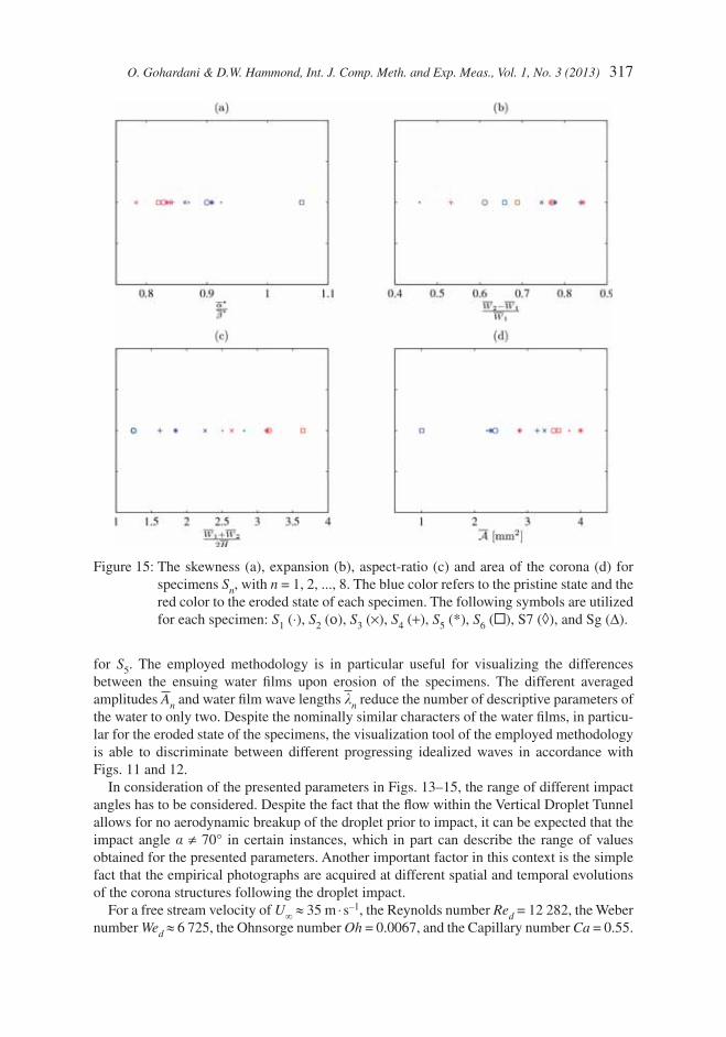
Due to the large number of parameters obtained, it is more fruitful to combine the param-eters to infer general trends about their behavior. Figure 15 shows the behavior of the corona structure based on its skewness, expansion, aspect ratio and area. It can be deduced that the majority of the specimens are skewed to the left in the pristine and eroded states respectively, apart from S6 which is skewed to the right prior to erosion. The plurality of the formed corona structures further expand in the eroded state.
The aspect ratio of the corona structures are further more rectangular in shape than square. It is also notable that the two-dimensional area of the corona structure occupies a larger area in the eroded state, in comparison to the virgin state of the material. This may be a conse-quence of the continuous water fi lm that is evident on most specimens in the aftermath of
316 O. Gohardani & D.W. Hammond, Int. J. Comp. Meth. and Exp. Meas., Vol. 1, No. 3 (2013)
erosion, allowing for more fl uid to become ejected from the surface upon impact. The DSWSAM methodology is also able to output dimensional parameters for the different fl uid characteristics. For the considered materials the averaged width and height of the beads with the corresponding standard deviation is given by w = 996.59 ± 298.46 and h = 298.12 ± 44.05 mm, respectively. The rivulets have an average width and height of x = 5300.44 and x = 113.38 mm. For the water fi lm the average wavelength and corresponding standard deviation is given by l = 1216.34 ± 135.35 mm. The averaged amplitude of the water fi lm and corre-sponding standard deviation is furthermore given by A = 204.344 ± 74.93 mm.
Given the fact that the DSWSAM represents various fl uid structures on a specimen surface by idealized representations, it can be established that there are deviations in shape and size between the encountered structures in comparison to the idealized representations. Despite the encountered differences however, the idealized structure are able to capture the hydropho-bic and hydrophilic nature of the specimens. The distance between the beads in particular, serves as an appropriate measure for establishing the extent of hydrophobicity of a surface. A large number of beads, placed adjacent to each other hence corresponds to a highly hydro-phobic surface as shown in Fig. 12(g) for the S8 specimen. An example of a less hydrophobic surface is depicted in Fig. 11(c) for S2. A hydrophilic surface is exemplifi ed by Fig. 12(a)
Figure 14: The angle a (a), angle b (b), a* (c) and b* (d) for specimens Sn, with n = 1, 2 , . . . , 8. The blue color refers to the pristine state and the red color to the eroded state of each specimen. The following symbols are utilized for each specimen: S1 (⋅), S2 (ο), S3 (×), S4 (+), S5 (*), S6 ( ), S7 (◊), and Sg (Δ).
O. Gohardani & D.W. Hammond, Int. J. Comp. Meth. and Exp. Meas., Vol. 1, No. 3 (2013) 317
for S5. The employed methodology is in particular useful for visualizing the differences between the ensuing water fi lms upon erosion of the specimens. The different averaged amplitudes An and water fi lm wave lengths ln reduce the number of descriptive parameters of the water to only two. Despite the nominally similar characters of the water fi lms, in particu-lar for the eroded state of the specimens, the visualization tool of the employed methodology is able to discriminate between different progressing idealized waves in accordance with Figs. 11 and 12.
In consideration of the presented parameters in Figs. 13–15, the range of different impact angles has to be considered. Despite the fact that the fl ow within the Vertical Droplet Tunnel allows for no aerodynamic breakup of the droplet prior to impact, it can be expected that the impact angle a ≠ 70° in certain instances, which in part can describe the range of values obtained for the presented parameters. Another important factor in this context is the simple fact that the empirical photographs are acquired at different spatial and temporal evolutions of the corona structures following the droplet impact.
For a free stream velocity of U∞ ≈ 35 m ⋅ s–1, the Reynolds number Red = 12 282, the Weber number Wed ≈ 6 725, the Ohnsorge number Oh = 0.0067, and the Capillary number Ca = 0.55.
Figure 15: The skewness (a), expansion (b), aspect-ratio (c) and area of the corona (d) for specimens Sn, with n = 1, 2, ..., 8. The blue color refers to the pristine state and the red color to the eroded state of each specimen. The following symbols are utilized for each specimen: S1 (⋅), S2 (ο), S3 (×), S4 (+), S5 (*), S6 ( ), S7 (◊), and Sg (Δ).
318 O. Gohardani & D.W. Hammond, Int. J. Comp. Meth. and Exp. Meas., Vol. 1, No. 3 (2013)
Table 2, shows the values of the boundary-layer thickness d99, displacement thickness d1, momentum thickness d2, and the energy thickness d3, wall shear stress tw, and skin-friction coeffi cient cf for different free stream velocities.
From Table 2 it is readily established that the approximate size of the boundary layer for a free stream velocity of 35 m ⋅ s–1 is approximately 463 mm. Therefore, a different structure behavior can be expected at the interface between the boundary layer fl ow and the outer fl ow.
The impact of a droplet onto a surface, at high velocities ensues in the growth of fi n-gers and their consequent breakup [18]. The growth of fi ngers around the periphery of the droplet during spreading is according to Allen [19], a result of the Rayleigh-Taylor Instability, which arises upon acceleration of the interface of fl uids with differing densi-ties. The Rayleigh- Taylor instability has in particular empirically been studied by utilizing a paramagnetic fl uid combination by Gohardani [20] and Gohardani et al. [21–23]. According to Aziz and Chandra [18], for high enough values resulting in splash-ing, the maximum spread factor %xmax .= 0 5
14Re and the number of fi ngers N, is given by
N K= ( )4 3 , with K Wed d= ( ){ }Re12
12
. Using these relations the maximum spread factor %xmax .≈ 5 26 and N ≈ 125.
5 CONCLUSIONSThe DSWSAM methodology is capable of capturing the qualitative observations of the wetting character of different surfaces adequately and express these features quantitatively. The usefulness of this developed methodology is evident upon comparison of nominally similar wetting characteristics of different materials. In particular, in this study the meth-odology has fully captured the wetting behavior of polymeric matrix composites reinforced with CNTs exhibiting a hydrophobic wetting character prior to erosion and a hydrophilic wetting character, post erosion. The potential role of erosion on the wettability of hydro-phobic surfaces is hence highlighted in this study. The change of surface character from a hydrophobic to a hydrophilic, can be of great importance in design aspects related to ice-phobic surfaces with applications within the aerospace industry. The developed methodology can further be adapted to incorporate more complex features, by addition of advanced modules.
ACKNOWLEDGMENTThe authors greatly acknowledge the fi nancial support from the European Union for conduct-ing this research as a part of multi-functional layers for safer aircraft composite structures (LAYSA) project, under the Seventh Framework Programme (FP7), including aeronautics.
Table 2: The boundary-layer thickness, displacement thickness, momentum thickness, energy thickness, wall shearstress and skin friction for different free stream velocities. All parameters are estimated for x = L, where L is the length of the specimen.
O. Gohardani & D.W. Hammond, Int. J. Comp. Meth. and Exp. Meas., Vol. 1, No. 3 (2013) 319
REFERENCES [1] Shalin, R.E., Polymer Matrix Composites. Springer, p. 440, 1995. ISBN 0412613301.
doi: http://dx.doi.org/10.1007/978-94-011-0515-6 [2] Gohardani, O., The infl uence of erosion and wear on the accretion and adhesion of ice
for nano reinforced polymeric composites used in aeronautics. Ph.D. Thesis, Cranfi eld University, United Kingdom, 2011.
[3] Gohardani, O., Impact of erosion testing aspects on current and future fl ight conditions. Progress in Aerospace Sciences, 47(4), Elsevier, pp. 280–303, 2011. doi:10.1016/j.paerosci.2011.04.001.
[4] Gohardani, O., Williamson, D.M. & Hammond, D.W., Multiple liquid impacts on polymeric matrix composites reinforced with carbon nanotubes. Wear, 294–295, pp. 336–346, 2012. doi:10.1016/j.wear.2012.07.007. doi: http://dx.doi.org/10.1016/j.wear.2012.07.007
[5] Gohardani O. & Hammond, D.W., Droplet interaction and dynamic wettability of advanced materials used in aeronautics. Presented at the 6th Subrata Chakrabarti International Conference on Fluid Structure Interaction, Fluid Structure Interaction May 9–11, 2011, Orlando, Florida, U.S.A.
[6] Gohardani, A.S., Doulgeris, G. & Singh, R., Challenges of future aircraft propulsion: a review of distributed propulsion technology and its potential application for the all electric commercial aircraft. Progress in Aerospace Sciences, 47(5), Elsevier, pp. 369–391, 2011. doi:10.1016/j.paerosci.2010.09.001. doi: http://dx.doi.org/10.1016/j.paerosci.2010.09.001
[7] Gohardani, A.S., A synergistic glance at the prospects of distributed propulsion technology and the electric aircraft concept for future unmanned air vehicles and commercial/military aviation. Progress in Aerospace Sciences, 2012. doi:10.1016/j.paerosci.2012.08.001.
[8] Gohardani A.S. & Gohardani O. Ceramic engine considerations for future aerospace propulsion. Aircraft Engineering and Aerospace Technology, 84(2), pp. 75–86, 2012. doi:10.1108/00022661211207884. doi: http://dx.doi.org/10.1108/00022661211207884
[9] Gohardani, O. & Hammond, D.W., Droplet interaction and dynamic wettability of advanced materials used in aeronautics. Advances in Fluid Mechanics IX, WIT Trans-actions on Engineering Sciences. ISBN 978-1-84564-600-4, pp. 175–185, 2012.
[10] Hammond, D.W., Luxford, G. & Ivey P., The Cranfi eld University Icing Tunnel. In: 41st AIAA Aerospace Sciences Meeting & Exhibit. 6–9 Jan 2003, Reno, U.S.A.
[11] Young, T., An essay on the cohesion of fl uids. Philosophical Transactions of The Royal Society London, 95, pp. 65–87, 1805. doi: http://dx.doi.org/10.1098/rstl.1805.0005
[12] Tadmor, R., Line energy and the relation between advancing, receding, and young contact angles. Langmuir, 20(18), pp. 7659 –7664, 2004. doi: http://dx.doi.org/10.1021/la049410h
[13] Ide, R.F., Comparison of Liquid Water Content measurement techniques in an icing wind tunnel. NASA/TM-1999-209643, 1999.
[14] Rein, M., Phenomena of liquid drop impact on solid and liquid surfaces. Fluid Dynamics Research, 12(2), pp. 61–93, 1993. doi: http://dx.doi.org/10.1016/0169-5983(93)90106-K
[15] Gonzalez, R.C., Woods, R.E. & Eddins, S.L., Digital Image Processing Using MATLAB, 2nd edn., Gatesmark Publishing, 2009. ISBN 9780982085400.
[16] Schlichting, H. & Gersten, K., Boundary-Layer Theory. Springer, 2000. ISBN 3-540-66270-7.
320 O. Gohardani & D.W. Hammond, Int. J. Comp. Meth. and Exp. Meas., Vol. 1, No. 3 (2013)
[17] Pasandideh-Fard, M., Qiao, Y.M., Chandra, S. & Mostaghimi, J., Capillary effects during droplet impact on a solid surface. Physics of Fluids, 8(3), pp. 650–659, 1996. doi: http://dx.doi.org/10.1063/1.868850
[18] Aziz, S.D. & Chandra, S., Impact, recoil and splashing of molten metal droplets. Inter-national Journal of Heat Mass Transfer, 43, pp. 2841–2857, 2000. doi: http://dx.doi.org/10.1016/S0017-9310(99)00350-6
[19] Allen, R.F. The role of surface tension in splashing. Journal of Colloid and Interface Science, 51, pp. 350–351, 1975. doi: http://dx.doi.org/10.1016/0021-9797(75)90126-5
[20] Gohardani, O., Experimental investigation of Rayleigh-Taylor instability using a para-magnetic liquid combination. M.Sc. Thesis, University of Arizona, U.S.A., 2008.
[21] Gohardani, O., Oemke, R. & Jacobs, J.W., PLIF fl ow visualization of magnetically stabilized Rayleigh-Taylor instability. American Physical Society, 59th Annual Meeting of the APS Division of Fluid Dynamics, November 19–21, 2006, Tampa Bay, Florida, U.S.A.
[22] Gohardani, O., Oemke, R. & Jacobs, J.W., Experimental study of Rayleigh-Taylor Instability utilizing a paramagnetic liquid combination. American Physical Society, 60th Annual Meeting of the APS Division of Fluid Dynamics, November 18–20, 2007. Salt Lake City, Utah, U.S.A.
[23] Gohardani, O. & Jacobs, J.W. Experimental investigation of the Rayleigh-Taylor Insta-bility using a paramagnetic liquid combination. Proceedings of the 11th International Workshop on the Physics of Compressible Turbulent Mixing (IWPCTM), July 13–18, 2008, Santa Fe, New Mexico, U.S.A.
[24] Gohardani, O., The Exploration of Icephobic Materials and Their Future Prospects in Aircraft Icing Applications. J Aeronaut Aerospace Eng, 1, p. e116, 2012. doi:10.4172/2168-9792.1000e116.