Dynamic Bargaining Markets and the Negative Swap Spread Preliminary and incomplete - Please do not quote! Sven Klingler * This draft: May 1, 2015 The difference between the yield of a government bond and the fixed rate in an interest rate swap is commonly referred to as swap spread. In 2008 the US swap spread for 30-year contracts turned negative. This is surprising because negative swap spreads are a theoretical arbitrage opportunity and unlike most other crisis phenomena the negative swap spread is very persistent. * Department of Finance and Center for Financial Frictions (FRIC). Copenhagen Business School, Solbjerg Plads 3, DK-2000 Frederiksberg, Denmark. E-mail: sk.fi@cbs.dk.
Transcript
Dynamic Bargaining Markets and the
Negative Swap SpreadPreliminary and incomplete - Please do not quote!
Sven Klingler∗
This draft: May 1, 2015
The difference between the yield of a government bond and the fixed rate in an
interest rate swap is commonly referred to as swap spread. In 2008 the US swap
spread for 30-year contracts turned negative. This is surprising because negative
swap spreads are a theoretical arbitrage opportunity and unlike most other crisis
phenomena the negative swap spread is very persistent.
∗ Department of Finance and Center for Financial Frictions (FRIC). Copenhagen Business School, SolbjergPlads 3, DK-2000 Frederiksberg, Denmark. E-mail: [email protected].
1. Introduction
During the financial crisis of 2007–2009 many pricing anomalies occurred in the financial
market. A common explanation for most of these anomalies is that a deterioration in funding
liquidity kept arbitrageurs from reinforcing the law of one price. Further, Lehman Brothers
was a large counterparty in the market for over-the-counter (OTC) derivatives. The default
of Lehman Brothers caused many derivatives dealers and end users to lose their counterparty
and put additional pressure on derivatives prices. The pricing anomaly that I study in this
paper is the negative swap spread. In September 2008, shortly after the default of Lehman
Brothers, the difference between the swap rate of a 30-year interest rate swap (IRS) and the
yield of a treasury bond with the same maturity, commonly referred to as swap spread, turned
negative. In contrast to other pricing anomalies, the 30-year swap spread is very persistent,
still trading at −10 basis points in February 2015.
Normally, swap spreads are a measure of uncertainty in the economy and increase in times
of market distress. The reason for this is twofold. First, in an IRS a fixed payment is
exchanged against a floating payment, which is typically based on Libor. Hence, even though
IRS are collateralized and viewed as free of counterparty credit risk, the swap rate should be
above the (theoretical) risk-free rate because of the credit risk in Libor. Hence, an increase
in bank credit risk, which increases the Libor rate, should increase the swap spread. Second,
treasuries have a status as safe and liquid assets and therefore carry a “convenience yield,”1
which means that the treasury yield is below the (theoretical) risk-free rate. If the uncertainty
in the economy increases, investors value the safety and liquidity of treasuries more, thereby
increasing the convenience yield. A higher convenience yield of treasuries causes the swap
spread to increase.
Given these considerations there are three puzzles regarding the negative swap spread.
First, why did the swap spread turn negative shortly after the default of Lehman Brothers?
This timing is surprising because both, Libor rates and the demand for safe and liquid assets
were at all-time heights which, according to the above considerations, should have increased
the swap spread. Second, why is the negative swap spread so persistent? Phrased differently,
what keeps arbitrageurs from reinforcing the law of one price here? It is difficult to explain
this long persistence with a lack of funding liquidity only, especially given that most other
pricing anomalies receded. Third, how can we explain the magnitude of the negative swap
spread? Since there is an arbitrage opportunity in negative swap spreads, the question is
who is willing to receive a swap rate below the corresponding treasury yield and why?
I argue that the solution to these puzzles is twofold. First, there is a difference in the
funding requirement for treasuries and IRS. The treasury requires initial funding while the
IRS has zero net present value. While this difference is almost irrelevant for sophisticated
investors who can use leverage and the repo market, it matters for less-sophisticated end-users
1See, for instance Krishnamurthy and Vissing-Jorgensen (2012) or Feldhutter and Lando (2008) for moredetails.
1
of the IRS. For example, corporations and pension funds could prefer IRS over treasuries.
Hence, the funding difference explains why there are customers willing to receive a swap
rate below the treasury yield. Second, selling IRS and hedging them using treasuries leaves
derivatives dealers exposed to a residual risk. In normal times, derivatives dealers would
enter the market and arbitrage the negative swap spread away. However, the default of
Lehman brothers can be interpreted as a severe shock to dealers’ risk-bearing capacity, which
kept them from selling IRS. Further, the possibility of such a severe shock, where it becomes
extremely costly to unwind existing IRS, explains why the swap spread did not converge back
to its original level.
I develop a model that explains negative swap spreads based on a supply-demand imbal-
ance. Derivatives dealers engage into IRS with customers to satisfy their demand. Customers
benefit from engaging in IRS by saving a certain hedge cost. This hedge cost could be in-
terpreted as the funding cost of a leverage-constrained investor buying treasuries instead of
using IRS. In normal times, the customer can get in contact with a dealer almost imme-
diately and is only willing to give a small fraction of c as a fee to the dealer. In a crisis,
the dealer’s risk-bearing capacity decreases and he is less able to provide the IRS. In this
case, it is more difficult for the customer to get in contact with a dealer. I interpret this
difficulty in obtaining an IRS as waiting time and build a search-theoretic model around this
supply-demand imbalance. The longer the waiting time, the more valuable the swap becomes
for the customer and the fraction of c that he is willing to pay as fee increases. Once the fee
increases above the theoretical frictionless swap spread, we observe negative swap spreads.
I provide four empirically findings to shed more light on the negative swap spread. First,
I show that the negative swap spread is an international phenomenon that also occurred in
Germany and Great Britain shortly after the default of Lehman Brothers. Second, using
quarterly macro-data in a regression analysis, I show that supply and demand variables
affect swap spreads. Third, I regress weekly changes in swap spreads after 2007 on several
explanatory variables, including sovereign CDS premia. It turns out that sovereign credit
risk, as measured by the CDS premium,2 does not explain 30-year swap spreads. Finally,
I use principal components analysis (PCA) to confirm that, after the default of Lehman
Brothers, the 30-year swap spread significantly differs from the other swap spreads.
1.1. Literature Review
Will be included in the next version.
2It is not obvious that CDS premia of safe sovereigns are a clean measure of credit risk. Klingler and Lando(2015) argue that safe-haven CDS premia are to a large extent driven by regulatory frictions.
2
2. Institutional Details
In an interest rate swap two parties agree on exchanging interest payments. The first party,
the fixed payer, receives a floating interest payment based on Libor every quarter. In turn, he
pays a fixed rate which is called the swap rate. This payment is typically done semi-annually.
The other party is called fixed receiver and has the opposite position, receiving the swap rate
and paying the Libor rate in turn. The position for the fixed receiver can be thought of as a
long position in a risk-free bond financed by a credit given at Libor rate which is rolled over
every quarter. The reason why the bond is viewed as risk-free is twofold. First, the swap is
typically collateralized. If the swap becomes a liability for one of the counterparties, he has to
post collateral to insure the other counterparty against losses in case of his default. Second,
there is no notional exchanged in the transaction. Hence, even if the counterparty defaults
and there is not enough collateral posted, the loss is much lower than in a comparable bond.
However, theory predicts that the fixed rate is slightly higher than a theoretical risk-free rate
because the bond purchase is financed at Libor, which contains a credit risk component.
Treasury securities on the other hand carry a “convenience yield”,3 meaning that they
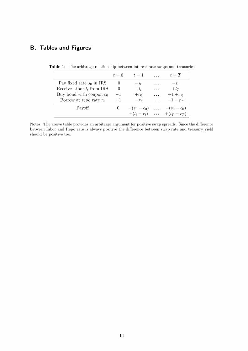
trade below the theoretical risk-free rate. The arbitrage argument in Table 1 illustrates that
there should be a positive swap spread. The fixed payer in an IRS buys a treasury bond
with the same maturity as the interest rate swap. To finance this transaction he uses a repo
transaction, where he uses the treasury as security to get a loan. He rolls over this repo
position every three months. Assuming no other frictions, that would give the following two
payment streams. A fixed stream of payments, receiving the treasury yield and paying the
swap rate and and a floating stream of payments, receiving the Libor rate and paying the
repo rate. The swap rate should be determined such that the fixed and floating payment
streams are equal. Since the difference between Libor and repo rate is always positive, the
difference between treasury yield and swap rate should be negative.
2.1. Limits to Negative Swap Spreads Arbitrage
The arbitrage strategy in Table 1 is subject to several frictions, most notably a funding
friction. In order to buy the treasury the arbitrageur has to borrow money using a repo
agreement. Treasuries with a maturity longer than 10 years are typically subject to a haircut
of approximately 6%,4 which means that the arbitrageur has to use some uncollateralized
funding for the position. Additionally to that, rolling over the repo agreement is subject
to the risk that the treasury security might decrease in value, in which case the arbitrageur
3See, for instance Krishnamurthy and Vissing-Jorgensen (2012) or Feldhutter and Lando (2008) for moredetails.
4This number is a first approximation that I obtained from http://www.cmegroup.com/clearing/
financial-and-collateral-management/. They analyze haircuts for securities posted as collateral incleared derivatives transactions. However, market participants confirm that 6% is a reasonable proxy forhaircuts of treasuries with 30 years to maturity.
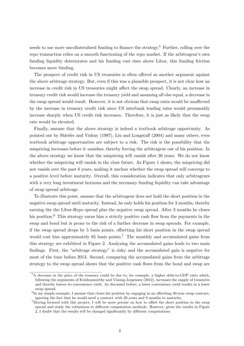
needs to use more uncollateralized funding to finance the strategy.5 Further, rolling over the
repo transaction relies on a smooth functioning of the repo market. If the arbitrageur’s own
funding liquidity deteriorates and his funding cost rises above Libor, this funding friction
becomes more binding.
The prospect of credit risk in US treasuries is often offered as another argument against
the above arbitrage strategy. But, even if this was a plausible prospect, it is not clear how an
increase in credit risk in US treasuries might affect the swap spread. Clearly, an increase in
treasury credit risk would increase the treasury yield and assuming all else equal, a decrease in
the swap spread would result. However, it is not obvious that swap rates would be unaffected
by the increase in treasury credit risk since US interbank lending rates would presumably
increase sharply when US credit risk increases. Therefore, it is just as likely that the swap
rate would be elevated.
Finally, assume that the above strategy is indeed a textbook arbitrage opportunity. As
pointed out by Shleifer and Vishny (1997), Liu and Longstaff (2004) and many others, even
textbook arbitrage opportunities are subject to a risk. The risk is the possibility that the
mispricing increases before it vanishes, thereby forcing the arbitrageur out of his position. In
the above strategy we know that the mispricing will vanish after 30 years. We do not know
whether the mispricing will vanish in the close future. As Figure 1 shows, the mispricing did
not vanish over the past 6 years, making it unclear whether the swap spread will converge to
a positive level before maturity. Overall, this consideration indicates that only arbitrageurs
with a very long investment horizons and the necessary funding liquidity can take advantage
of swap spread arbitrage.
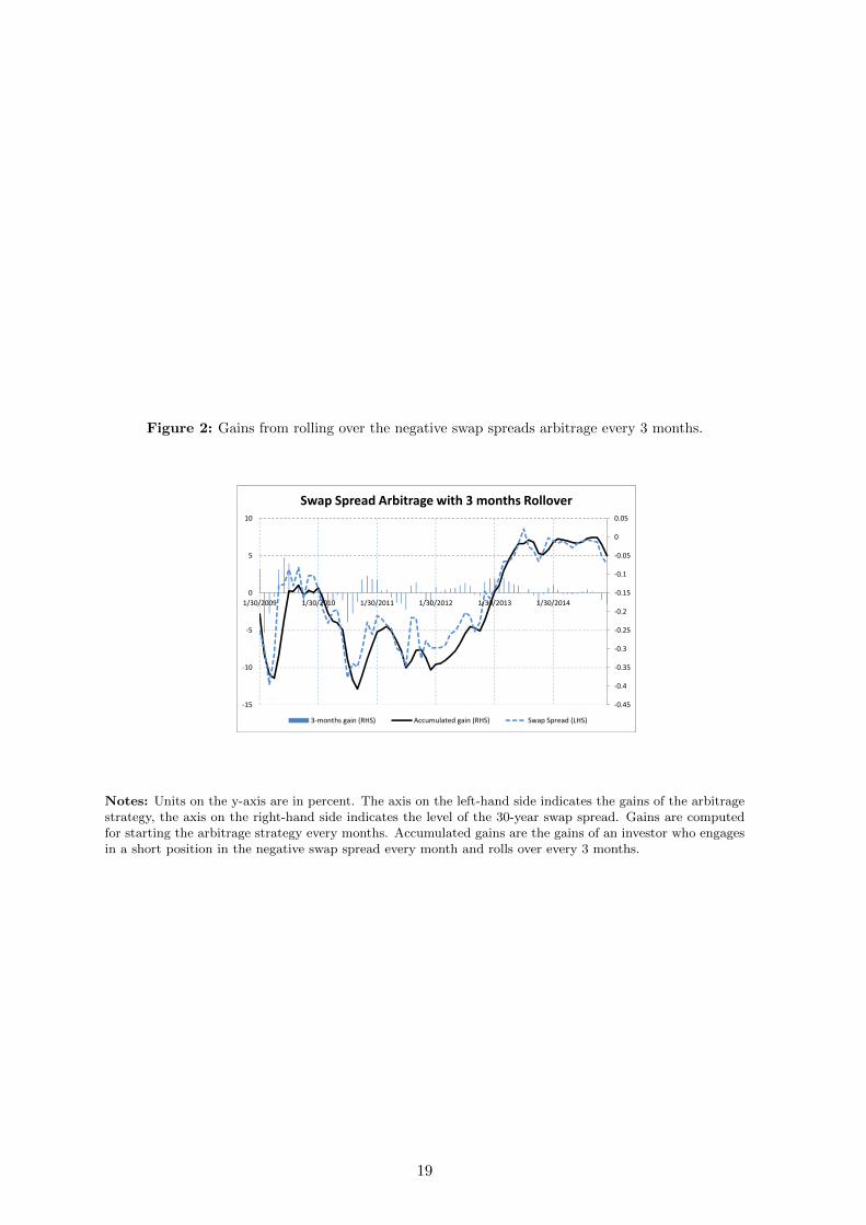
To illustrate this point, assume that the arbitrageur does not hold the short position in the
negative swap spread until maturity. Instead, he only holds his position for 3 months, thereby
earning the the Libor-Repo spread plus the negative swap spread. After 3 months he closes
his position.6 This strategy earns him a strictly positive cash flow from the payments in the
swap and bond but is prone to the risk of a further decrease in swap spreads. For example,
if the swap spread drops by 5 basis points, offsetting his short position in the swap spread
would cost him approximately 85 basis points.7 The monthly and accumulated gains from
this strategy are exhibited in Figure 2. Analyzing the accumulated gains leads to two main
findings. First, the “arbitrage strategy” is risky and the accumulated gain is negative for
most of the time before 2013. Second, comparing the accumulated gains from the arbitrage
strategy to the swap spread shows that the positive cash flows from the bond and swap are
5A decrease in the price of the treasury could be due to, for example, a higher debt-to-GDP ratio which,following the arguments of Krishnamurthy and Vissing-Jorgensen (2012), increases the supply of treasuriesand thereby lowers its convenience yield. As discussed before, a lower convenience yield results in a lowerswap spread.
6In my simple example, I assume that closes his position by engaging in an offsetting 30-year swap contract,ignoring the fact that he would need a contract with 29 years and 9 months to maturity.
7Moving forward with this project, I will be more precise on how to offset the short position in the swapspread and study the robustness to different computation methods. However, given the results in Figure2, I doubt that the results will be changed significantly by different computations
4
dwarfed by the costs of exiting the short position in the negative swap spread.
2.2. The Demand and Supply of Interest Rate Swaps
Engaging in an interest rate swap with a new counterparty is subject to several requirements.
For instance, both parties need to set up an ISDA master agreement which takes time.
Therefore, customers usually establish a trading relationship with one or several derivatives
dealers and do not trade directly with each other. If the demand for paying fixed and
receiving fixed is balanced, the dealer simply acts as an intermediary. In this case there
would be no demand pressure and the dealer simply extracts a bid-ask spread. If there is an
excess demand for one of the two positions the dealer takes the other side of the transaction,
thereby warehousing the swap and supplying swaps to investors.
Investors use IRS for speculation or hedging purposes. In both cases the demand for IRS
can depend on the level and the slope of the yield curve. The level of the yield curve matters,
for instance, for agencies issuing Mortgage-Backed Securities (MBS). Agencies aim to balance
the duration of their assets and liabilities. When interest rates fall, mortgage borrowers tend
to execute their prepayment right, thereby lowering the duration of the agencies’ mortgage
portfolio. Hence agencies want to receive fixed in an IRS to hedge this mortgage prepayment
risk.8 The slope of the yield curve matters for non-financial firms. According to Faulkender
(2005), these firms tend to use IRS mostly for speculation, preferring to pay floating when
the yield curve is steep. Faulkender (2005) also finds that firms tend to prefer paying fixed
when macro-economic conditions worsen.
Overall, the above examples show that there could be demand and supply effects in the
interest rate swap market. Customers, like non-financial firms, could have a demand for
paying or for receiving fixed. However, it is unlikely that firms have a large demand for IRS
with a maturity of 30 years, where the negative swap spread still persists. The most important
customers in the long end of the swap curve are pension funds and insurance companies, who
have a natural demand for receiving fixed for longer tenors. Pension funds have long-term
liabilities towards their clients and the Pension Protection Act of 2006 requires them to
match the duration of their asset portfolios with the duration of these liabilities. Increasing
the duration of their asset portfolios could be achieved by receiving fixed in an IRS or by
buying bonds with long maturities.9 However, Ang, Chen, and Sundaresan (2013) find that
many US pension funds are underfunded and tend to more risky investments. To this end,
they prefer to use the funding required to buy long-term bonds for buying risky assets. Hence,
they have a demand for receiving fixed in an IRS.
Another common argument for negative swap spreads is that buying treasuries requires
capital while an IRS has zero present value. For a sophisticated investor with full access to
8Feldhutter and Lando (2008) argue that using IRS is the predominant way for doing this as opposed tousing treasuries.
9Greenwood and Vayanos (2010) provide evidence from the 2004 pension reform in the United Kingdomwhere pension funds started buying long-dated gilts.
5
repo financing, buying a treasury requires a minor initial funding of approximately 6%, as
discussed before. At the same time, engaging in an IRS could also require an initial margin
and regular collateral posting. Therefore, this funding difference is not a limit to the above
arbitrage strategy. However, for less-sophisticated investors who need to balance their asset-
liability duration and do not have access to repo financing or have severe leverage constraints,
this argument is important. These investors value IRS more than treasuries because IRS are
a cheaper way for them to balance their asset-liability duration. Therefore, they are willing
to receive a swap rate which is below the fair swap rate. I argue in the following section that
the size of this “fee” depends on how easily they can find a trader that is willing to provide
them with an IRS.
3. The Model
The market for IRS is dominated by a small amount of dealers and finding a dealer is straight
forward. In normal times a customer calls his dealer(s) and they start negotiating the swap
rate without much delay.10 When the dealer is in financial distress, or his risk-bearing
capacity is low, the customer has to wait before he starts negotiating the rate with his dealer.
One interpretation is that the dealer needs to check with his risk-management if he is able
to provide the swap before he trades. If risk management does not allow the dealer to trade
there will be a significant waiting time for the customer. In this case, the customer either tries
calling his dealer again later or establishes a new trading relationship with another dealer.
As noted before, establishing a new trading relationship takes time.
The mechanism that explains negative swap spreads in my model is as follows. Customers
benefit from engaging in IRS by saving a cost c. This cost could be interpreted as the funding
cost of a leverage-constrained investor buying treasuries instead of using IRS. In normal times,
the customer can get in contact with a dealer almost immediately and is only willing to give
a small fraction of c as a fee to the dealer. When dealers’ risk-bearing capacity decreases or
when there is an excessive demand for IRS by customers, it takes longer for the customer
to get in contact with a dealer. The longer the waiting time, the more valuable the swap
becomes for the customer and the fraction of c that he is willing to pay as fee increases. Once
the fee increases above the fair swap spread we observe negative swap spreads.
3.1. Model Setup
There are two kinds of agents in the baseline model, derivatives dealers and and customers.
Both agents are impatient at the same rate r. A fraction µ of the customers needs to engage
in a receiver IRS to heighten their portfolio duration. I abstract from the dealer’s role as
intermediary and focus on the case where the dealer provides the IRS as fixed payer to a
10In practice, dealers post indicative quotes at which they are willing to trade. After customers get in contactwith a dealer the indicative quote typically gets adjusted. I interpret this as a bargaining game.
6
customer. Hence, µ can be interpreted as excess demand for receiving fixed in an IRS by
customers. If a customer successfully engages in a IRS he avoids a constant stream of costs
c.11 A fraction ν of dealers is in the market and ready to provide the IRS to the customers.
Customers get in contact with dealers at a rate α(θ), which depends on the amount of available
dealers relative to the demand for IRS (θ = ν/µ). For providing the IRS to the customer,
the derivatives dealer charges a fee φ.
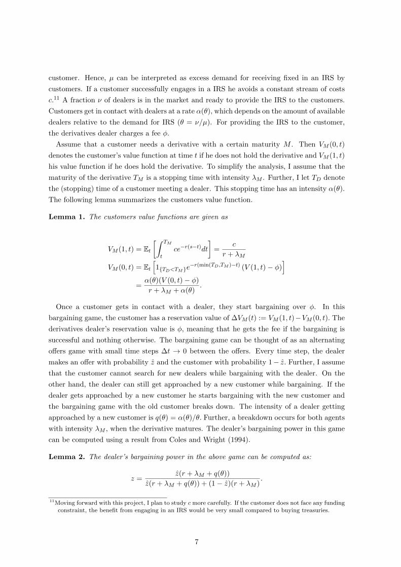
Assume that a customer needs a derivative with a certain maturity M . Then VM (0, t)
denotes the customer’s value function at time t if he does not hold the derivative and VM (1, t)
his value function if he does hold the derivative. To simplify the analysis, I assume that the
maturity of the derivative TM is a stopping time with intensity λM . Further, I let TD denote
the (stopping) time of a customer meeting a dealer. This stopping time has an intensity α(θ).
The following lemma summarizes the customers value function.
Lemma 1. The customers value functions are given as
VM (1, t) = Et[∫ TM
tce−r(s−t)dt
]=
c
r + λM
VM (0, t) = Et[1{TD<TM}e
−r(min(TD,TM )−t) (V (1, t)− φ)]
=α(θ)(V (0, t)− φ)
r + λM + α(θ).
Once a customer gets in contact with a dealer, they start bargaining over φ. In this
bargaining game, the customer has a reservation value of ∆VM (t) := VM (1, t)−VM (0, t). The
derivatives dealer’s reservation value is φ, meaning that he gets the fee if the bargaining is
successful and nothing otherwise. The bargaining game can be thought of as an alternating
offers game with small time steps ∆t → 0 between the offers. Every time step, the dealer
makes an offer with probability z and the customer with probability 1− z. Further, I assume
that the customer cannot search for new dealers while bargaining with the dealer. On the
other hand, the dealer can still get approached by a new customer while bargaining. If the
dealer gets approached by a new customer he starts bargaining with the new customer and
the bargaining game with the old customer breaks down. The intensity of a dealer getting
approached by a new customer is q(θ) = α(θ)/θ. Further, a breakdown occurs for both agents
with intensity λM , when the derivative matures. The dealer’s bargaining power in this game
can be computed using a result from Coles and Wright (1994).
Lemma 2. The dealer’s bargaining power in the above game can be computed as:
z =z(r + λM + q(θ))
z(r + λM + q(θ)) + (1− z)(r + λM ).
11Moving forward with this project, I plan to study c more carefully. If the customer does not face any fundingconstraint, the benefit from engaging in an IRS would be very small compared to buying treasuries.
7
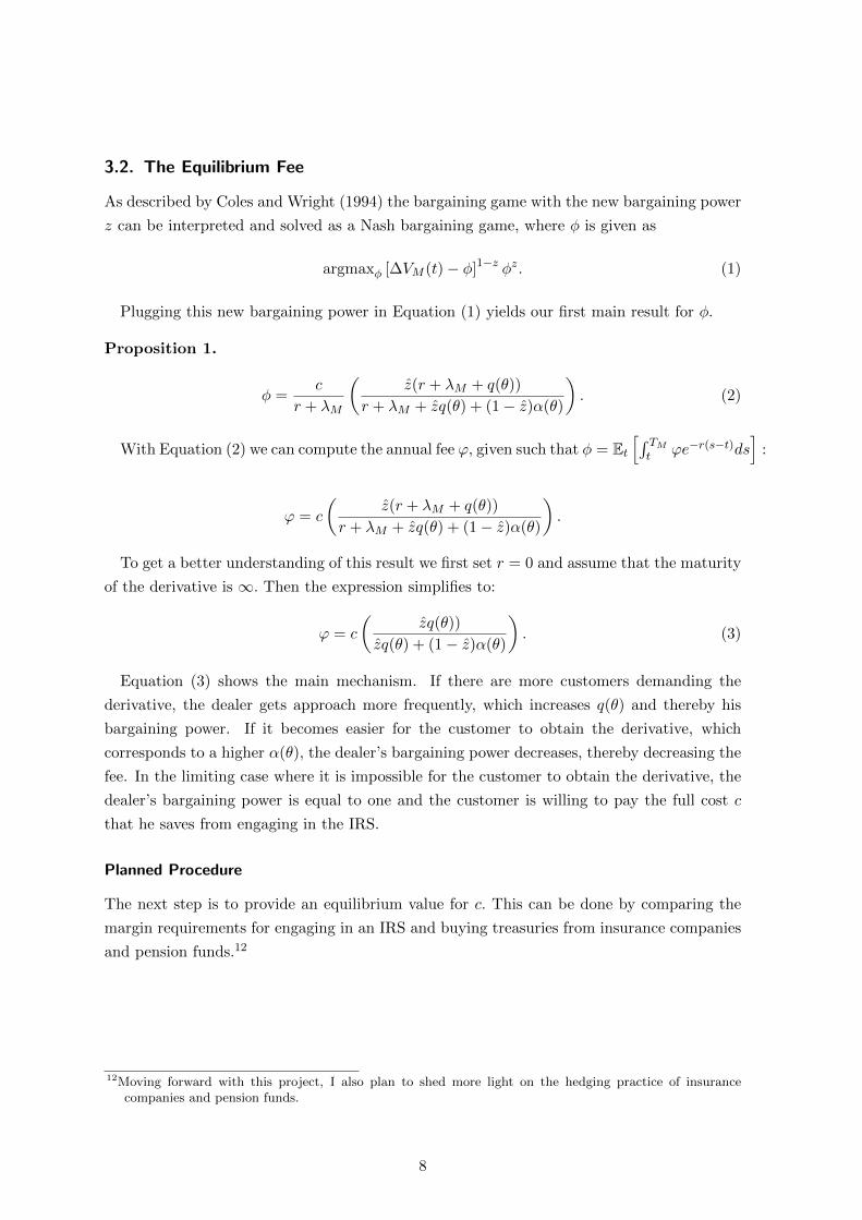
3.2. The Equilibrium Fee
As described by Coles and Wright (1994) the bargaining game with the new bargaining power
z can be interpreted and solved as a Nash bargaining game, where φ is given as
argmaxφ [∆VM (t)− φ]1−z φz. (1)
Plugging this new bargaining power in Equation (1) yields our first main result for φ.
Proposition 1.
φ =c
r + λM
(z(r + λM + q(θ))
r + λM + zq(θ) + (1− z)α(θ)
). (2)
With Equation (2) we can compute the annual fee ϕ, given such that φ = Et[∫ TMt ϕe−r(s−t)ds
]:
ϕ = c
(z(r + λM + q(θ))
r + λM + zq(θ) + (1− z)α(θ)
).
To get a better understanding of this result we first set r = 0 and assume that the maturity
of the derivative is ∞. Then the expression simplifies to:
ϕ = c
(zq(θ))
zq(θ) + (1− z)α(θ)
). (3)
Equation (3) shows the main mechanism. If there are more customers demanding the
derivative, the dealer gets approach more frequently, which increases q(θ) and thereby his
bargaining power. If it becomes easier for the customer to obtain the derivative, which
corresponds to a higher α(θ), the dealer’s bargaining power decreases, thereby decreasing the
fee. In the limiting case where it is impossible for the customer to obtain the derivative, the
dealer’s bargaining power is equal to one and the customer is willing to pay the full cost c
that he saves from engaging in the IRS.
Planned Procedure
The next step is to provide an equilibrium value for c. This can be done by comparing the
margin requirements for engaging in an IRS and buying treasuries from insurance companies
and pension funds.12
12Moving forward with this project, I also plan to shed more light on the hedging practice of insurancecompanies and pension funds.
8
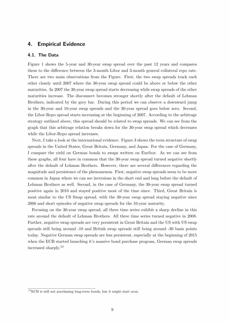
4. Empirical Evidence
4.1. The Data
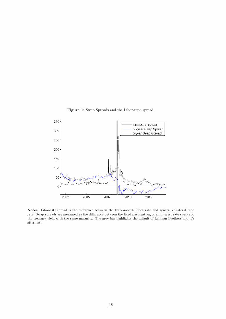
Figure 1 shows the 5-year and 30-year swap spread over the past 12 years and compares
them to the difference between the 3-month Libor and 3-month general collateral repo rate.
There are two main observations from the Figure. First, the two swap spreads track each
other closely until 2007 where the 30-year swap spread could be above or below the other
maturities. In 2007 the 30-year swap spread starts decreasing while swap spreads of the other
maturities increase. The disconnect becomes stronger shortly after the default of Lehman
Brothers, indicated by the grey bar. During this period we can observe a downward jump
in the 30-year and 10-year swap spreads and the 30-year spread goes below zero. Second,
the Libor-Repo spread starts increasing at the beginning of 2007. According to the arbitrage
strategy outlined above, this spread should be related to swap spreads. We can see from the
graph that this arbitrage relation breaks down for the 30-year swap spread which decreases
while the Libor-Repo spread increases.
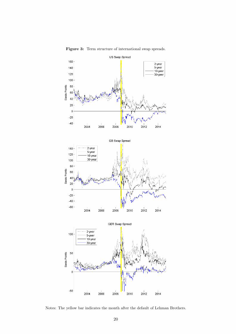
Next, I take a look at the international evidence. Figure 3 shows the term structure of swap
spreads in the United States, Great Britain, Germany, and Japan. For the case of Germany,
I compare the yield on German bonds to swaps written on Euribor. As we can see from
these graphs, all four have in common that the 30-year swap spread turned negative shortly
after the default of Lehman Brothers. However, there are several differences regarding the
magnitude and persistence of the phenomenon. First, negative swap spreads seem to be more
common in Japan where we can see inversions in the short end and long before the default of
Lehman Brothers as well. Second, in the case of Germany, the 30-year swap spread turned
positive again in 2010 and stayed positive most of the time since. Third, Great Britain is
most similar to the US Swap spread, with the 30-year swap spread staying negative since
2008 and short episodes of negative swap spreads for the 10-year maturity.
Focusing on the 30-year swap spread, all three time series exhibit a sharp decline in this
rate around the default of Lehman Brothers. All three time series turned negative in 2008.
Further, negative swap spreads are very persistent in Great Britain and the US with US swap
spreads still being around -10 and British swap spreads still being around -30 basis points
today. Negative German swap spreads are less persistent, especially at the beginning of 2015
when the ECB started launching it’s massive bond purchase program, German swap spreads
increased sharply.13
13ECB is still not purchasing long-term bonds, but it might start soon.
9
4.2. Regression Analysis
Macro Variables
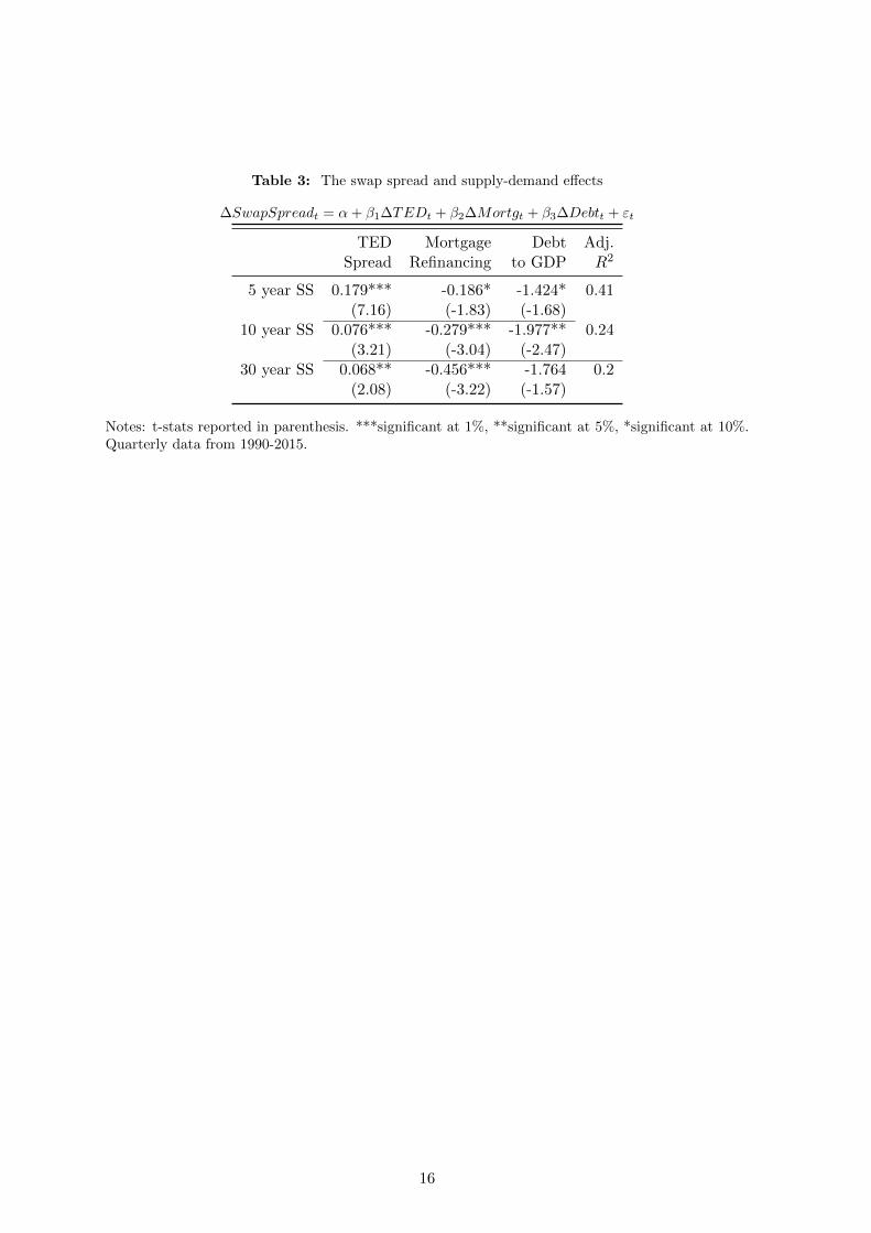
To take a first look at the evidence, I regress changes in the 5-year, 10-year, and 30-year
swap spread on three different explanatory variables. First, the difference between the 3-
month Libor and 3-month treasury yield, commonly referred to as TED spread. This variable
captures the Libor-repo spread and a specialness component of treasuries. As we can see from
Table 3, swap spreads tend to increase when the TED spread increases. Further, we can see
that the effect is less significant for the long end. Second, following the logic of Feldhutter and
Lando (2008), I argue that mortgage issuers need IRS to balance their asset-liability duration
when mortgage refinancing rates change. This demand is proxied by the mortgage refinancing
rate, measured by the mortgage banker association. The regression shows that an increase
of mortgage refinancing rates corresponds to a decrease in swap spreads, indicating that a
higher demand for receiving fixed decreases the swap spread. Finally, I use the US Debt-
to-GDP ratio as a proxy for the convenience yield in treasuries. Following Krishnamurthy
and Vissing-Jorgensen (2012), the idea is that when there is more supply of treasuries the
convenience yield decreases, thereby decreasing the swap spread. We can see from Table 3
that an increase in the debt-to-GDP ratio indeed lowers the swap spread.
CDS and other Market Variables
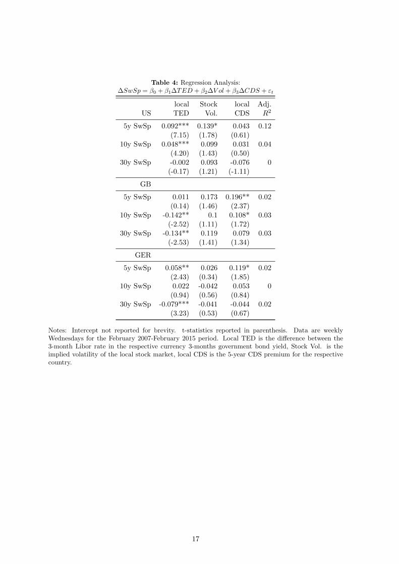
Table 4 shows the results of regressing changes in swap spreads of different maturities on three
explanatory variables. First, changes in the difference between the 3-month Libor rate in the
respective currency and the 3-month government bond yield. Second, the implied volatility
of the local stock market return and third, the respective sovereign CDS premium. There are
two main findings from this analysis. First, the local TED spread tends to be a significant
explanatory variable for short-term swap spreads. Surprisingly, for 30-year swap spreads the
local TED spread is significant for Germany and Great Britain but with a negative coefficient.
This implies that increases in the local TED spread coincide with decreases in the 30-year
swap spread. This is a surprising finding and goes against the arbitrage argument provided
above. Second, sovereign credit risk is not a significant explanatory variable for most of the
swap spreads. In the case of the United States and Germany, the coefficient of the CDS
premium has the wrong sign, but is insignificant.
4.2.1. Changes in Regressions Before and After Lehman
Will be included in the next version.
4.3. Principal Components Analysis
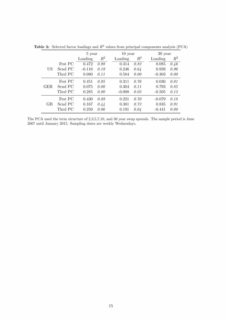
In this section, I document first document that the 30 year swap spread is significantly
different from the other swap spreads in the term structure. To this end, table 2 shows
10
the factor loadings and R2 values of from a principal components analysis (PCA) of the
swap spreads term structure for the February 2007 to February 2015 period. For all three
countries, the factor loadings for the 30-year swap spread differ significantly from the other
factor loadings exhibited in the table. 5-year and 10-year swap spreads are to a large extent
explained by the first principal component while both the factor loading and R2 value is
much smaller for the 30-year swap spread. The 30-year swap spread for all three sovereigns
in the sample is loading heavier on the second principal component than the first, indicating
a different time-series behaviour.
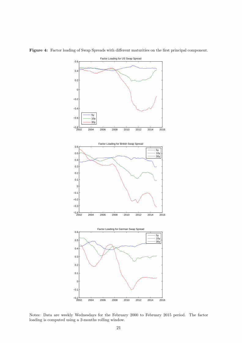
The second empirical finding documented in this section is that the factor loading has
changed over the past years, especially after the default of Lehman Brothers. To document
this fact, I use a rolling-PCA approach. In particular, I use data from February 2000 until
February 2015 and compute the factor loading on the first principal component for the 5, 10,
and 30-year swap spread for a rolling window of 2 years. The results of this computation are
exhibited in Figure 4. Again, for all three sovereigns the pattern looks similar. The three
factor loadings track each other closely until 2008. Afterwards, there is a sharp decline in the
factor loading of the 30-year swap spread. Overall, these PCAs document that the behaviour
30-year swap spread differs significantly from the behaviour of the other swap spreads and
that this difference was not there before 2008.
5. Conclusion
Will be included in the next version.
11
References
Ang, A., B. Chen, and S. Sundaresan (2013). Liability investment with downside risk.
Technical report, National Bureau of Economic Research.
Coles, M. G. and R. Wright (1994). Dynamic bargaining theory. Technical report, Federal
Reserve Bank of Minnesota, Research Department.
Faulkender, M. (2005). Hedging or market timing? selecting the interest rate exposure of
corporate debt. The Journal of Finance 60 (2), 931–962.
Feldhutter, P. and D. Lando (2008). Decomposing swap spreads. Journal of Financial
Economics 88 (2), 375–405.
Krishnamurthy, A. and A. Vissing-Jorgensen (2012). The aggregate demand for treasury
debt. Journal of Political Economy 120 (2), 233–267.
Liu, J. and F. A. Longstaff (2004). Losing money on arbitrage: Optimal dynamic portfolio
choice in markets with arbitrage opportunities. Review of Financial Studies 17 (3),
611–641.
Shleifer, A. and R. W. Vishny (1997). The limits of arbitrage. The Journal of Fi-
nance 52 (1), 35–55.
12
A. Proofs
Will be included in the next version.
13
B. Tables and Figures
Table 1: The arbitrage relationship between interest rate swaps and treasuries
t = 0 t = 1 . . . t = T
Pay fixed rate s0 in IRS 0 −s0 . . . −s0Receive Libor lt from IRS 0 +lt . . . +lTBuy bond with coupon c0 −1 +c0 . . . +1 + c0
Notes: The above table provides an arbitrage argument for positive swap spreads. Since the differencebetween Libor and Repo rate is always positive the difference between swap rate and treasury yieldshould be positive too.
14
Table 2: Selected factor loadings and R2 values from principal components analysis (PCA)
5 year 10 year 30 yearLoading R2 Loading R2 Loading R2
Frst PC 0.472 0.98 0.314 0.82 0.085 0.46US Scnd PC -0.116 0.19 0.246 0.64 0.939 0.96
Thrd PC 0.080 0.11 0.584 0.00 -0.303 0.00
Frst PC 0.451 0.95 0.311 0.76 0.030 0.01GER Scnd PC 0.075 0.00 0.304 0.11 0.793 0.85
Thrd PC 0.285 0.00 -0.008 0.03 -0.505 0.12
Frst PC 0.430 0.89 0.221 0.70 -0.079 0.18GB Scnd PC 0.167 0.44 0.381 0.73 0.835 0.91
Thrd PC 0.250 0.06 0.191 0.04 -0.441 0.08
The PCA used the term structure of 2,3,5,7,10, and 30 year swap spreads. The sample period is June2007 until January 2015. Sampling dates are weekly Wednesdays.
15
Table 3: The swap spread and supply-demand effects
Notes: Intercept not reported for brevity. t-statistics reported in parenthesis. Data are weeklyWednesdays for the February 2007-February 2015 period. Local TED is the difference between the3-month Libor rate in the respective currency 3-months government bond yield, Stock Vol. is theimplied volatility of the local stock market, local CDS is the 5-year CDS premium for the respectivecountry.
17
Figure 1: Swap Spreads and the Libor-repo spread.
Notes: Libor-GC spread is the difference between the three-month Libor rate and general collateral reporate. Swap spreads are measured as the difference between the fixed payment leg of an interest rate swap andthe treasury yield with the same maturity. The grey bar highlights the default of Lehman Brothers and it’saftermath.
18
Figure 2: Gains from rolling over the negative swap spreads arbitrage every 3 months.
3‐months gain (RHS) Accumulated gain (RHS) Swap Spread (LHS)
Notes: Units on the y-axis are in percent. The axis on the left-hand side indicates the gains of the arbitragestrategy, the axis on the right-hand side indicates the level of the 30-year swap spread. Gains are computedfor starting the arbitrage strategy every months. Accumulated gains are the gains of an investor who engagesin a short position in the negative swap spread every month and rolls over every 3 months.
19
Figure 3: Term structure of international swap spreads.
Notes: The yellow bar indicates the month after the default of Lehman Brothers.
20
Figure 4: Factor loading of Swap Spreads with different maturities on the first principal component.
2002 2004 2006 2008 2010 2012 2014 2016−0.8
−0.6
−0.4
−0.2
0
0.2
0.4
0.6Factor Loading for US Swap Spread
5y10y30y
2002 2004 2006 2008 2010 2012 2014 2016−0.4
−0.3
−0.2
−0.1
0
0.1
0.2
0.3
0.4
0.5
0.6Factor Loading for British Swap Spread
5y10y30y
2002 2004 2006 2008 2010 2012 2014 2016−0.2
−0.1
0
0.1
0.2
0.3
0.4
0.5
0.6Factor Loading for German Swap Spread
5y10y30y
Notes: Data are weekly Wednesdays for the February 2000 to February 2015 period. The factorloading is computed using a 2-months rolling window.