Pritthi ChattopadhyayDepartment of Mechanical and

Nuclear Engineering,

Pennsylvania State University,

University Park, PA 16802

e-mail: pritthichatterjee@gmail.com

Sudeepta MondalDepartment of Mechanical and

Nuclear Engineering,

Pennsylvania State University,

University Park, PA 16802

e-mail: sudeepta979@gmail.com

Chandrachur BhattacharyaDepartment of Mechanical and

Nuclear Engineering,

Pennsylvania State University,

University Park, PA 16802

e-mail: chandrachur.bhattacharya@gmail.com

Achintya MukhopadhyayDepartment of Mechanical Engineering,

Jadavpur University,

Kolkata 700 032, India

e-mail: achintya.mukho@gmail.com

Asok Ray1

Fellow ASME

Department of Mechanical and

Nuclear Engineering,

Pennsylvania State University,

University Park, PA 16802

e-mail: axr2@psu.edu

Dynamic Data-Driven Design ofLean Premixed Combustors forThermoacoustically StableOperationsPrediction of thermoacoustic instabilities is a critical issue for both design and operationof combustion systems. Sustained high-amplitude pressure and temperature oscillationsmay cause stresses in structural components of the combustor, leading to thermomechan-ical damage. Therefore, the design of combustion systems must take into account thedynamic characteristics of thermoacoustic instabilities in the combustor. From this per-spective, there needs to be a procedure, in the design process, to recognize the operatingconditions (or parameters) that could lead to such thermoacoustic instabilities. However,often the available experimental data are limited and may not provide a complete map ofthe stability region(s) over the entire range of operations. To address this issue, a Bayes-ian nonparametric method has been adopted in this paper. By making use of limitedexperimental data, the proposed design method determines a mapping from a set of oper-ating conditions to that of stability regions in the combustion system. This map isdesigned to be capable of (i) predicting the system response of the combustor at operat-ing conditions at which experimental data are unavailable and (ii) statistically quantify-ing the uncertainties in the estimated parameters. With the ensemble of information thusgained about the system response at different operating points, the key design parametersof the combustor system can be identified; such a design would be statistically significantfor satisfying the system specifications. The proposed method has been validated withexperimental data of pressure time-series from a laboratory-scale lean-premixed swirl-stabilized combustor apparatus. [DOI: 10.1115/1.4037307]

Keywords: dynamic data-driven application, symbolic dynamics, combustion instability,uncertainty quantification

1 Introduction

Thermoacoustic instabilities result from the coupling betweenunsteady heat release rate and acoustic pressure fluctuations insidethe combustion chamber [1,2]. Design optimization of combustorsis a challenging problem due to the difficulties in modeling thenonlinear dynamics involved in thermoacoustic instabilities.These difficulties limit the application of model-based design opti-mization to combustion systems that involve several input param-eters (e.g., inlet velocity of air, air-fuel ratio, premixing level, andcombustor geometry) [3–5]; these parameters potentially affectthe combustion dynamics. Examples are existence of bifurcationsin the dynamic behavior of combustors and extremely high sensi-tivity of the combustor behavior to even small changes in some ofthe design parameters. On the other hand, it is economically infea-sible and unrealistic to have sensors for online measurements ofall dynamic variables involved in combustion and to conductexperiments at a sufficiently dense set of operating points. Tradi-tional design of combustion systems has focused on issues likeefficiency, power generation, and emission [3,4]. However, withthe implementation of low emission technologies like lean pre-mixed combustion, combustors have to operate in regimes wherethey are prone to thermoacoustic instabilities. The instabilityproblems have been aggravated by use of newer grades of fuelslike biofuels and hydrogen-based fuels like synthetic gas, because

these fuels have energy content and heat release pattern, whichare widely different from those of conventional hydrocarbon fuels.Consequently, the behavior of the system becomes significantlyaltered in terms of phenomena like occurrence of instabilities,blowout, and flashback. Thermoacoustic instability is alsoencountered in rocket engines.

The current state-of-the-art of mitigating combustion instabil-ities at the design stage itself mostly involves introduction of pas-sive devices, such as quarter wave tube arrangement [6] andperforated liners [7]. These devices improve the stability of thesystem by damping the oscillations in the combustion chamber.However, the use of passive devices can be only partially success-ful in mitigating different types of anomalous behavior as thesepassive devices are not designed on the basis of actual perform-ance of the combustor. An alternative approach that has been gain-ing popularity is the implementation of active control devices/mechanisms, where appropriate actions are initiated like injectionof secondary fuel [8–10]. These strategies are primarily designedto alter the phase difference between the pressure and heat-release-rate oscillations. Due to the complexity of the physicsinvolved, control algorithms often use data-driven methods. How-ever, implementation of these strategies in real time is challengingas the underlying dynamics is extremely fast (e.g., in the order ofkilohertz for some of the circumferential modes of instability ingas turbine afterburners). Another method of avoiding combustioninstabilities is identification of the stable operating zone at thedesign stage itself and limiting the parameter space of the designvariables to the stable operating zone only. The most commonlyfollowed approach for such predictive modeling is the networkmodel [11], where the combustor is resolved into a network of

1Corresponding author.Contributed by the Design Automation Committee of ASME for publication in

the JOURNAL OF MECHANICAL DESIGN. Manuscript received February 20, 2017; finalmanuscript received June 19, 2017; published online October 2, 2017. Assoc. Editor:Yan Wang.

Journal of Mechanical Design NOVEMBER 2017, Vol. 139 / 111419-1Copyright VC 2017 by ASME

Downloaded From: http://mechanicaldesign.asmedigitalcollection.asme.org/ on 11/02/2017 Terms of Use: http://www.asme.org/about-asme/terms-of-use

interconnected simpler elements and the response of each compo-nent to specific units is studied. To account for the complex flamedynamics, which is highly nonlinear, the linear transfer functionapproach is generalized to development of “flame describingfunction” [12]. The flame describing function, which describes aninput–output relation for the flame element, is usually derivedfrom experiments or computational fluid dynamics analysis. How-ever, the network model and the flame describing function, in par-ticular, have limitations in predicting different dynamic regimesof a combustor. With the availability of increasing computingpower, high fidelity computer simulations have also been used forpredicting the dynamic behavior [13]. Nevertheless, these simula-tions can be too time-consuming and computationally expensiveto use as a design tool.

An alternative approach for combustor design has been pro-posed in this paper. Data generated from limited number of runsunder diverse operating conditions have been used to generate theknowledge base about the system dynamics, which has then beenused for designing the combustor system. Although such a data-driven approach has been used quite extensively for characterizingand controlling the combustor dynamics [14,15], dynamic data-driven approach for designing combustors from the viewpoint ofthermoacoustic stability is rather uncommon.

Recently, the concept of dynamic data-driven application sys-tems (DDDAS) [16] has found its way into design methodologiesdue to the advent of fast sensing and computational technologiesas well as due to the inherent flexibility of DDDAS. Both quanti-tative and qualitative data have been used in various fields ofdesign, where a given software or program analyzes the collecteddata to produce a decision that would aid in the design of the sys-tem under consideration. Especially the dynamic characterizationof the system evolution allows for continual optimization of thedesign space as new data become available, thus enhancing theoverall design quality. In particular, the notion of DDDAS hasbeen used in the field of combustion monitoring and control. In arecent work, DDDAS has been used for the prediction of instabil-ity and flame lean-blow-out in combustors [14,15] using symbolictime series analysis (STSA) [17]. More recently, such an imaging-based analysis has also been reported using neural networks,where flame images have been used to detect the onset of combus-tion instability [18] also using STSA.

From the previously mentioned perspectives, this paper pro-poses a novel method of combustor design that is built upon theconcept of DDDAS [16], instead of completely relying on model-based design tools. The proposed design method only needs lim-ited amounts of process data in the form of time series and doesnot require any detailed knowledge of the underlying combustiondynamics. Given the information in the form of time series data atcertain operating conditions, a Bayesian nonparametric statisticalmethod has been adopted to predict the system behavior for oper-ating conditions at which data may not be available. In addition,the algorithm also quantifies the confidence in the estimate of thesystem response. The design algorithm produces a mapping froma set of operating conditions to that of stability regions in the com-bustion system. Once this map is generated, combustor designerscan use it for predicting the system response by statistically quan-tifying the uncertainties at operating conditions for which experi-mental data may not be available. This information facilitates theidentification of the combustion system parameters, which willallow the design to be statistically significant in terms of satisfy-ing the system specifications.

In the present work, experimental data from a laboratory-scaleswirl-premixed combustor apparatus have been used to generate astability map in the parameter space. To do this, time series dataof pressure oscillations at different combinations of combustorlength, equivalence ratio (/), and inlet flow velocities have beenconsidered. Using the limited data at hand, the devised algorithmcreates a stability map, which can then predict the systemresponse for an unknown set of parameters of combustor length,equivalence ratio, and inlet flow velocities. This provides the

designer with an estimate of the probability of the system at newparameters to become unstable, without the need for actualexperimentation.

The objective here is prediction of combustion instabilities inorder to prevent serious structural damage in the combustor.Hence, the user must design a combustor with a smaller probabil-ity of becoming unstable, which translates to the following tworequirements:

(1) Extraction of a feature that is highly sensitive to deviationsin the underlying state of the system from the nominal state.Then, even a small deviation in the system behavior fromthe nominal state would be manifested as a large featuredivergence.

(2) Quantification of the uncertainty in the estimate of the sys-tem stability for unknown parameters (e.g., combustorlength). This would help the user to make the parameterchoice, which would have a significantly reduced probabil-ity of resulting in an unstable system.

From the previously mentioned perspectives, major contribu-tions and innovations of the paper are summarized below:

(1) Development of a dynamic data-driven method for combus-tor design, based on STSA [17,19], which satisfies theabove two requirements.

(2) Validation of the above method on experimental data froma swirl-stabilized combustor apparatus [20].

The paper is organized in six sections including the abstract andintroduction. Section 2 describes the combustor apparatus that hasbeen used to generate time series data. Section 3 develops theproposed dynamic data-driven algorithm for combustor design.Section 4 describes the procedure and results of validation of theproposed algorithm on the experimental data. Section 5summarizes the work and delineates possible directions for futureresearch.

2 Description of the Experimental Apparatus

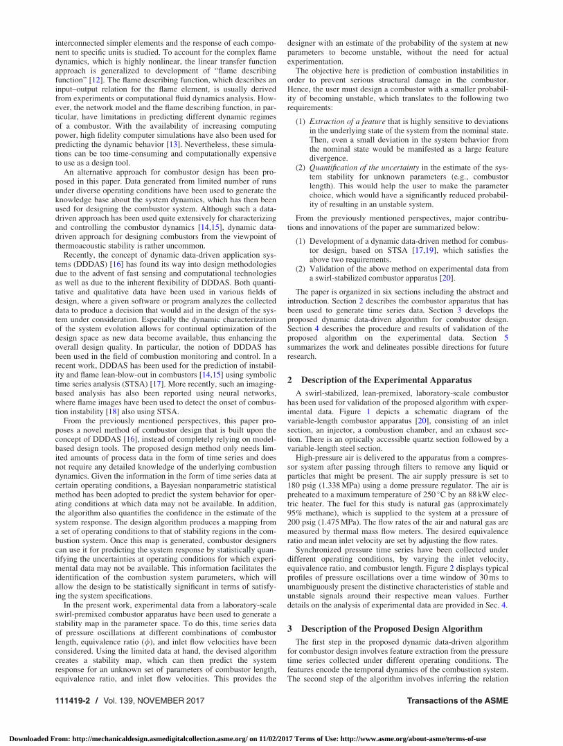
A swirl-stabilized, lean-premixed, laboratory-scale combustorhas been used for validation of the proposed algorithm with exper-imental data. Figure 1 depicts a schematic diagram of thevariable-length combustor apparatus [20], consisting of an inletsection, an injector, a combustion chamber, and an exhaust sec-tion. There is an optically accessible quartz section followed by avariable-length steel section.

High-pressure air is delivered to the apparatus from a compres-sor system after passing through filters to remove any liquid orparticles that might be present. The air supply pressure is set to180 psig (1.338 MPa) using a dome pressure regulator. The air ispreheated to a maximum temperature of 250 �C by an 88 kW elec-tric heater. The fuel for this study is natural gas (approximately95% methane), which is supplied to the system at a pressure of200 psig (1.475 MPa). The flow rates of the air and natural gas aremeasured by thermal mass flow meters. The desired equivalenceratio and mean inlet velocity are set by adjusting the flow rates.

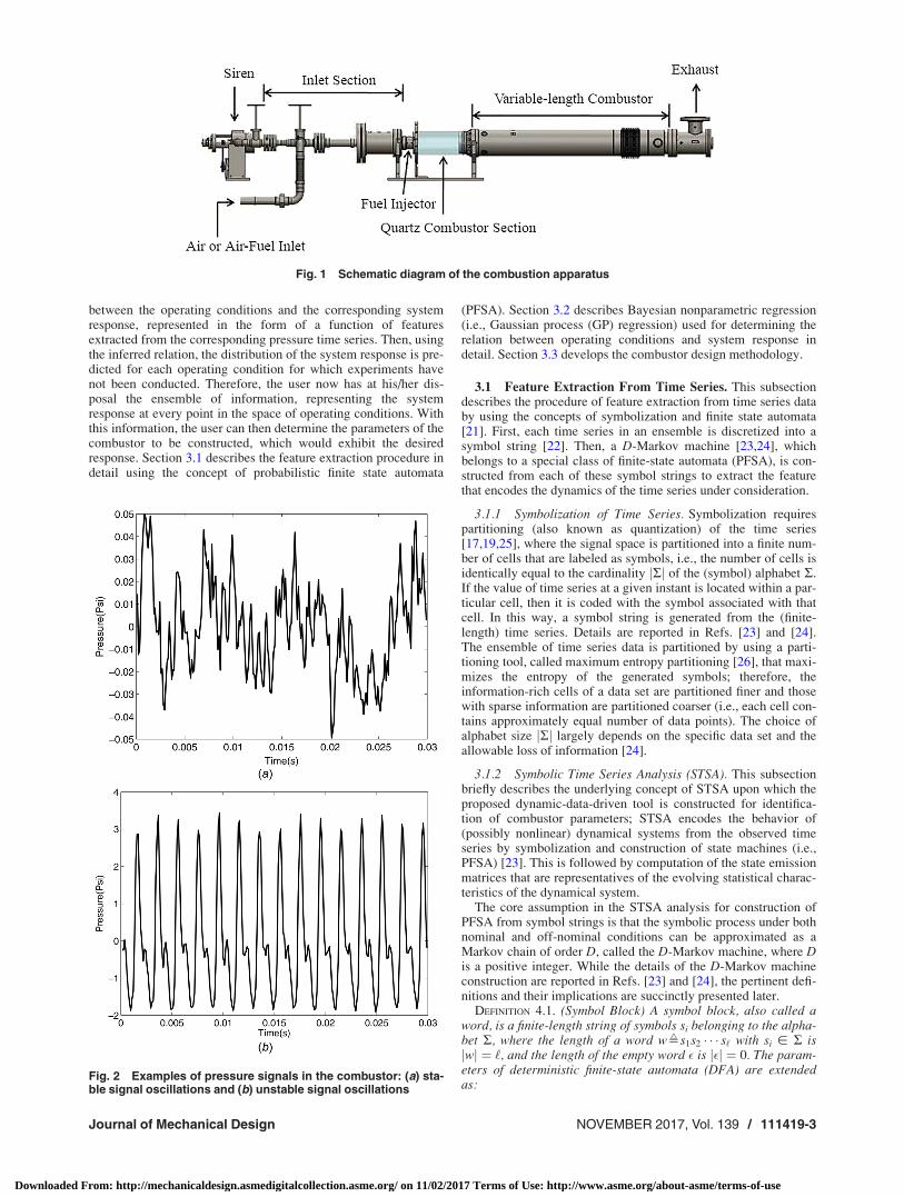
Synchronized pressure time series have been collected underdifferent operating conditions, by varying the inlet velocity,equivalence ratio, and combustor length. Figure 2 displays typicalprofiles of pressure oscillations over a time window of 30 ms tounambiguously present the distinctive characteristics of stable andunstable signals around their respective mean values. Furtherdetails on the analysis of experimental data are provided in Sec. 4.

3 Description of the Proposed Design Algorithm

The first step in the proposed dynamic data-driven algorithmfor combustor design involves feature extraction from the pressuretime series collected under different operating conditions. Thefeatures encode the temporal dynamics of the combustion system.The second step of the algorithm involves inferring the relation

111419-2 / Vol. 139, NOVEMBER 2017 Transactions of the ASME

Downloaded From: http://mechanicaldesign.asmedigitalcollection.asme.org/ on 11/02/2017 Terms of Use: http://www.asme.org/about-asme/terms-of-use

between the operating conditions and the corresponding systemresponse, represented in the form of a function of featuresextracted from the corresponding pressure time series. Then, usingthe inferred relation, the distribution of the system response is pre-dicted for each operating condition for which experiments havenot been conducted. Therefore, the user now has at his/her dis-posal the ensemble of information, representing the systemresponse at every point in the space of operating conditions. Withthis information, the user can then determine the parameters of thecombustor to be constructed, which would exhibit the desiredresponse. Section 3.1 describes the feature extraction procedure indetail using the concept of probabilistic finite state automata

(PFSA). Section 3.2 describes Bayesian nonparametric regression(i.e., Gaussian process (GP) regression) used for determining therelation between operating conditions and system response indetail. Section 3.3 develops the combustor design methodology.

3.1 Feature Extraction From Time Series. This subsectiondescribes the procedure of feature extraction from time series databy using the concepts of symbolization and finite state automata[21]. First, each time series in an ensemble is discretized into asymbol string [22]. Then, a D-Markov machine [23,24], whichbelongs to a special class of finite-state automata (PFSA), is con-structed from each of these symbol strings to extract the featurethat encodes the dynamics of the time series under consideration.

3.1.1 Symbolization of Time Series. Symbolization requirespartitioning (also known as quantization) of the time series[17,19,25], where the signal space is partitioned into a finite num-ber of cells that are labeled as symbols, i.e., the number of cells isidentically equal to the cardinality jRj of the (symbol) alphabet R.If the value of time series at a given instant is located within a par-ticular cell, then it is coded with the symbol associated with thatcell. In this way, a symbol string is generated from the (finite-length) time series. Details are reported in Refs. [23] and [24].The ensemble of time series data is partitioned by using a parti-tioning tool, called maximum entropy partitioning [26], that maxi-mizes the entropy of the generated symbols; therefore, theinformation-rich cells of a data set are partitioned finer and thosewith sparse information are partitioned coarser (i.e., each cell con-tains approximately equal number of data points). The choice ofalphabet size jRj largely depends on the specific data set and theallowable loss of information [24].

3.1.2 Symbolic Time Series Analysis (STSA). This subsectionbriefly describes the underlying concept of STSA upon which theproposed dynamic-data-driven tool is constructed for identifica-tion of combustor parameters; STSA encodes the behavior of(possibly nonlinear) dynamical systems from the observed timeseries by symbolization and construction of state machines (i.e.,PFSA) [23]. This is followed by computation of the state emissionmatrices that are representatives of the evolving statistical charac-teristics of the dynamical system.

The core assumption in the STSA analysis for construction ofPFSA from symbol strings is that the symbolic process under bothnominal and off-nominal conditions can be approximated as aMarkov chain of order D, called the D-Markov machine, where Dis a positive integer. While the details of the D-Markov machineconstruction are reported in Refs. [23] and [24], the pertinent defi-nitions and their implications are succinctly presented later.

DEFINITION 4.1. (Symbol Block) A symbol block, also called aword, is a finite-length string of symbols si belonging to the alpha-bet R, where the length of a word w¢s1s2 � � � s‘ with si � R isjwj ¼ ‘, and the length of the empty word � is j�j ¼ 0. The param-eters of deterministic finite-state automata (DFA) are extendedas:

Fig. 1 Schematic diagram of the combustion apparatus

Fig. 2 Examples of pressure signals in the combustor: (a) sta-ble signal oscillations and (b) unstable signal oscillations

Journal of Mechanical Design NOVEMBER 2017, Vol. 139 / 111419-3

Downloaded From: http://mechanicaldesign.asmedigitalcollection.asme.org/ on 11/02/2017 Terms of Use: http://www.asme.org/about-asme/terms-of-use

(1) The set of all words constructed from symbols in R, includ-ing the empty word �, is denoted as R?,

(2) The set of all words, whose suffix (respectively, prefix) isthe word w, is denoted as R?w (respectively, wR?).

(3) The set of all words of (finite) length ‘, where ‘> 0, isdenoted as R‘.

DEFINITION 4.2. A deterministic finite-state automaton (DFSA) Gis a triple R;Q; dð Þ [27], where:

(1) R is a (nonempty) finite alphabet with cardinality jRj;(2) Q is a (nonempty) finite set of states with cardinality jQj;(3) d : Q� R! Q is the state transition map.

DEFINITION 4.3. A probabilistic finite-state automaton (PFSA) isconstructed on the algebraic structure of deterministic finite stateautomata (DFA) G ¼ R;Q; dð Þ as a pair K¼ (G, P), i.e., thePFSA K is a four-tuple K ¼ R;Q; d;Pð Þ [23,24], where:

(1) R is a nonempty finite set, called the symbol alphabet, withcardinality jRj <1;

(2) Q ¼ fq1; q2;…; qjQjg is the state set with cardinality

jQj � jRjD, i.e., the states are represented by equivalenceclasses of symbol blocks of maximum length D correspond-ing to a symbol sequence S.

(3) d : Q� R! Q is the state transition mapping, whichgenerates the symbol sequences;

(4) P : Q� R! 0; 1½ � is the morph matrix of size jQj � jRj;the ijth element P(i, j) of the matrix P denotes the proba-bility of finding the symbol rj at next time step while mak-ing a transition from the state qi.

3.1.3 D-Markov Modeling. This subsection introduces a spe-cial class of PFSA, called D-Markov machine, which has a simplealgebraic structure and is computationally efficient for construc-tion and implementation [23,24].

DEFINITION 4.4. (D-Markov) A D-Markov machine [23] is aPFSA in which each state is represented by a (nonempty) finitestring of D symbols where

(1) D, a positive integer, is the depth of the Markov machine;(2) Q is the finite set of states with cardinality jQj � jRjD. The

states are represented by equivalence classes of symbolstrings of maximum length D, and each symbol in the stingbelongs to the alphabet R;

(3) d: Q�R! Q is the state transition map that satisfies thefollowing condition if jQj ¼ jRjD: There exist a, b � R ands � R? such that d(as, b)¼ sb and as, sb � Q.

Remark 4.1. It follows from Definition 4.4 that a D-Markovchain is treated as a statistically stationary stochastic processS ¼ � � � s�1s0s1 � � �, where the probability of occurrence of a newsymbol depends only on the last D symbols, i.e., P snj � � � sn�D½� � � sn�1� ¼ P snjsn�D � � � sn�1½ �.

The construction of a D-Markov machine is based on (i) statesplitting that generates symbol blocks of different lengths accord-ing to their relative importance and (ii) state merging that assimi-lates histories from symbol blocks leading to the same symbolicbehavior. Words of length D on a symbol string are treated as thestates of the D-Markov machine before any state-merging is exe-cuted. Thus, on an alphabet R, the total number of possible statesbecomes less than or equal to jRjD; and operations of state merg-ing may significantly reduce the number of states [24]. However,no state splitting or state merging is required for D¼ 1, which isthe simplest configuration of a D-Markov machine.

The PFSA states represent different combinations of blocks ofsymbols on the symbol string. In the graph of a PFSA, the direc-tional edge (i.e., the emitted event) that interconnects a state (i.e.,a node) to another state represents the transition probabilitybetween these states. Therefore, the “states” denote all possiblesymbol blocks (i.e., words) within a window of certain length, andthe set of all states is denoted as Q ¼ fq1; q2;…; qjQjg and jQj is

the number of (finitely many) states. The procedure for estimationof the emission probabilities is presented next.

Given a (finite length) symbol string S over a (finite) alphabet R,there exist several PFSA construction algorithms to discover theunderlying irreducible PFSA model K of S. These algorithms startwith identifying the structure of the PFSA K¢ Q;R; d;pð Þ. To esti-mate the state emission matrix, a jQj � jRj count matrix C is con-structed and each element ckj of C is computed as: ckj¢1þ Nkj,where Nkj denotes the number of times that a symbol rj is gener-ated from the state qk upon observing the symbol string S. Themaximum a posteriori probability estimates of emission probabil-ities for PFSA K are computed by frequency counting as

p rjjqk

� �¢

ckjP‘ ck‘¼ 1þ Nkj

jRj þP

‘ Nkj(1)

The rationale for initializing each element of the count matrix Cto 1 is that if no event is generated at a state q � Q, then thereshould be no preference to any particular symbol and it is logicalto have p rjqð Þ ¼ 1=jRjð Þ 8r 2 R, i.e., the uniform distribution ofevent generation at the state q. The above procedure guaranteesthat the PFSA, constructed from a (finite-length) symbol string,must have an (elementwise) strictly positive emissivity map P.

Having computed the emission probabilities p rjjqk

� �for j 2

f1; 2;…; jRjg and k 2 f1; 2;…; jQjg, the estimated jQj � jRjð Þemission probability matrix of the PFSA is obtained as

P¢

p r1jq1ð Þ … p rjRjjq1

� �� . .

.�

p r1jqjQj� �

� � � p rjRjjqjQj� �

2664

3775 (2)

Bahrampour et al. [25] presented a comparative evaluation ofCepstrum, principal component analysis (PCA) and STSA as fea-ture extractors for target detection and classification. The underly-ing algorithms of feature extraction were executed in conjunctionwith three different pattern classification algorithms, namely, sup-port vector machines (SVM), k-nearest neighbor, and sparse rep-resentation classifier. The results of comparison show consistentlysuperior performance of STSA-based feature extraction over bothCepstrum-based and PCA-based feature extraction in terms ofsuccessful detection, false alarm, and wrong detection and classifi-cation decisions. Similar results on superior performance of STSAover PCA have been reported by Mallapragada et al. [28] forrobotic applications. Rao et al. [29] reported a review of STSAand its performance evaluation relative to other classes of patternrecognition tools, such as Bayesian filters and artificial neuralnetworks.

Section 3.2 describes the methodology for determining themapping between operating conditions and system response as afunction of the estimated emission probability matrix P that istaken to be the extracted feature.

3.2 Gaussian Process Regression. This section describes thetechnique used for determining the relation between operatingconditions and the system responses as a function of the featuresextracted in Sec. 3.1. This relation is then used for predicting theresponses for operating conditions for which experiments havenot been conducted.

Given a set of operating conditions and the correspondingcontinuous-valued system responses, there exist several regressionalgorithms in the machine learning literature (e.g., see Ref. [30]),which infer the underlying relation between the conditions andresponse, under different assumptions on the characteristics of therelation. The inferred relation can then be used to predict theresponse of an unseen system condition (i.e., whose response isunknown). In contrast, Gaussian process (GP) regression [31] is anonparametric method that can model arbitrary relations betweenthe condition and response without making any specific

111419-4 / Vol. 139, NOVEMBER 2017 Transactions of the ASME

Downloaded From: http://mechanicaldesign.asmedigitalcollection.asme.org/ on 11/02/2017 Terms of Use: http://www.asme.org/about-asme/terms-of-use

assumptions on the relation. In addition, most regression algo-rithms only provide point estimates of the response, but they donot quantify the confidence in that estimate. Being a Bayesianmethod, GP also quantifies the uncertainties in the predictionsresulting from possible measurement noise and errors in theparameter estimation procedure. Hence, GP regression has beenadopted in this paper to infer the relation between the operatingconditions and the corresponding system response.

3.2.1 Theory of Gaussian Process Regression. This subsec-tion succinctly presents the underlying theory of Gaussian process(GP) regression. Further details are available in standard literature(e.g., see Ref. [31]).

A stochastic process is a collection of random variables,fn tð Þ : t 2 Tg, where T is an index set. A Gaussian process is a sto-chastic process such that any finite collection of random variableshas a multivariate jointly Gaussian distribution. In particular, acollection of random variables fn tð Þ : t 2 Tg is said to be drawnfrom a Gaussian process with mean function m(�) and covariancefunction k(�, �) if, for any finite set of elements t1,…, tl � T, thecorresponding random variables n(t1),…, n(tl) have multivariatejointly Gaussian distribution

n t1ð Þ::

n tlð Þ

24

35 � N

m t1ð Þ::m tlð Þ

24

35; k t1; t1ð Þ…k t1; tlð Þ

::k tl; t1ð Þ…k tl; tlð Þ

24

35

0@

1A

0@ (3)

where m tð Þ¢E n tð Þ½ � is the mean function and k t; t0ð Þ¢E n tð Þ � m tð Þð Þ n t0ð Þ � m t0ð Þ

� �� �is the covariance function.

Equation (3) is denoted in vector notation as: n � GP m;K� �

. The

GP regression algorithm is now described below.Let X¼ {xi} and Y ¼ fyig; i ¼ 1;…; n, be the training data set,

where X denotes a set of operating conditions and Y denotes thecorresponding set of system responses. The objective here is todetermine the relation between X and Y so that, given an unknownoperating condition x, the corresponding system response y can bepredicted. In the GP regression algorithm, it is assumed thaty¼ n(x)þ e, where e is independent and identically distributed(iid) (additive) noise, N(0, r2). That is, the response y is assumedto be a stochastic process that is a function of the operating condi-tion x with additive noise. Then, a zero-mean Gaussian processprior GP 0;K

� �is assumed for the function n. By the property of

GP in Eq. (3)), the marginal distribution over any set of operatingconditions belonging to X must be multivariate jointly Gaussian.Thus, given a set {xk1, xk2,…xkm}, the corresponding {n(xk1),n(xk2),…n(xkm)} has a multivariate jointly Gaussian distribution.Hence, by concatenating the training and testing sets of operatingconditions as: [X, Xtest], the marginal distribution of their respec-tive system responses [n(X), n(Xtest)] is also multivariate jointlyGaussian. Thus, the training and testing responses are jointly dis-tributed as

n Xð Þn Xtestð Þ

� �� N 0;

K X;Xð Þ K X;Xtestð ÞK Xtest;Xð Þ K Xtest;Xtestð Þ

� �� (4)

where n Xð Þ¼ n x1ð Þ;…;n xnð Þ� �0; n Xtestð Þ¼ n xtest

1

� �;…;n xtest

m

� �h i0;

K X;Xtestð Þ 2Rn�m such that K X;Xtestð Þð Þij¼ k xi;xtestj

�; K X;Xð Þ 2

Rn�n such that K X;Xð Þð Þij¼ k xi;xjð Þ; K Xtest;Xtestð Þ 2Rm�m such

that K Xtest;Xtestð Þð Þij¼ k xtesti ;xtest

j

�; K Xtest;Xð Þ 2Rm�n such that

K Xtest;Xð Þð Þij¼ k xtesti ;xj

� �.

Since the system responses Y and Ytest are contaminated with

additive iid Gaussian noise, i.e.,e

etest

� �� N 0;

r2I 0

0 r2I

� �� where e ¼ e1;…; en

� �0; and etest ¼ e1

test;…; emtest

� �0, it follows that

Y

Ytest

" #¼

n

ntest

" #þ

e

etest

" #

�N 0;K X;Xð Þ þ r2I K X;Xtestð ÞK Xtest;Xð Þ K Xtest;Xtestð Þ þ r2I

" # !(5)

where Ytest ¼ ytest1 ;…; ytest

m

� �0. The rules for conditioning on Gaus-

sians, YtestjY � N ltest;Rtest� �

yield

ltest ¼ K Xtest;X� �

K X;Xð Þ þ r2I� ��1

Y (6)

Rtest ¼ K Xtest;Xtest� �

þ r2I

�K Xtest;X� �

K X;Xð Þ þ r2I� ��1

K X;Xtest� �

(7)

Thus, the algorithm predicts the mean and variance of the systemresponse for every test condition. Instead of a zero-mean prior(i.e., E[n(x)]¼ 0), a mean function m(x) could also be incorpo-rated into the prior. In such a case

ltest ¼ m Xtestð Þ þ K Xtest;X� �

K X;Xð Þ þ r2I� ��1

Y � m Xð Þð Þ (8)

instead of Eq. (6), and Rtest remains unchanged in Eq. (7).

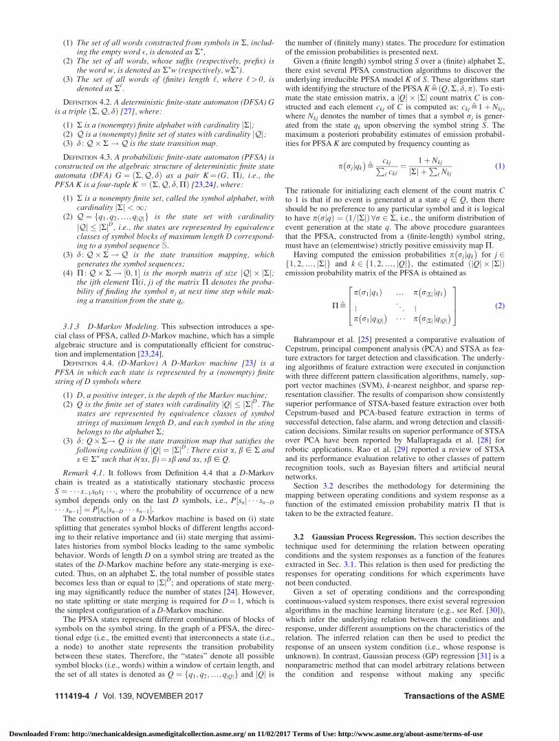
3.3 Development of the Design Methodology. This subsec-tion develops the combustor design methodology by combiningthe algorithms, described in Secs. 3.1 and 3.2. Figure 3 presents aflowchart of the proposed combustor design algorithm, whileSec. 4 explains the details along with a discussion on experimentalresults.

4 Experimental Validation of the Design Method

This section validates the algorithms, developed in Sec. 3, onthe data collected from an experimental apparatus that isdescribed in Sec. 2. Synchronized time series data of pressureoscillations have been collected under different operating condi-tions, by varying the following parameters:

(1) Inlet velocity from 25 to 50 m/s in steps of 5 m/s.(2) Equivalence ratio (/) as 0.525, 0.550, 0.600, and 0.650.(3) Combustor length from 25 to 59 in in steps of 1 in.

Time series data of pressure oscillations have been collected ata sampling rate of 8192 Hz for each of the above 6� 4� 35¼ 840distinct operating conditions. The time span of data collection hasbeen 8 s (i.e., 65,536 measurement data per channel) for each timeseries, which is within the safe limit of operation of the combustorapparatus and which is long enough to provide sufficient informa-tion for statistical analysis. The root-mean-square (rms) value,Prms, of pressure has been calculated for each time series. Forthis data set, an observed ground truth is that all systems withPrms 0.07 psi are unstable, while all those with Prms< 0.07 psiare stable. Although Prms appears to serve as a good indicator ofstability in this set of experiments, a natural question ariseswhether Prms could be universally adopted as a feature. SincePrms is the standard deviation of the signal in the statistical sense,it is sensitive to noise. Therefore, Prms may not be an ideal choiceas a feature, because of its lack of robustness to measurementnoise.

In the design of a real-life combustor, sufficiently long dura-tions of data acquisition might not be feasible due to various chal-lenges inflicted on the system performance and operability (e.g.,high-amplitude pressure and temperature oscillations, and localair–fuel ratio variations leading to flame blowout) specifically dur-ing combustion instabilities. Figure 4 shows representative plotsof Prms calculated for different durations of time series in incre-ments of 0.1 s for (a) a stable signal and (b) an unstable signal. It

Journal of Mechanical Design NOVEMBER 2017, Vol. 139 / 111419-5

Downloaded From: http://mechanicaldesign.asmedigitalcollection.asme.org/ on 11/02/2017 Terms of Use: http://www.asme.org/about-asme/terms-of-use

is shown in Fig. 4(a) that the threshold Prms of 0.07 psi isexceeded at time series window lengths ranging from about 2.5 sto 4 s. Although Prms over the entire 8 s window is less than thethreshold of 0.07 psi, an online stability criterion based on solely aPrms threshold may generate false alarms for those durations,where the threshold is exceeded. Similar conclusions can bedrawn from Fig. 4(b) where, for an actually unstable signal, Prmsdrops below 0.07 psi within several time windows between 1 s to3 s and close to 4 s. In both cases, a hard Prms threshold is likelyto yield misclassifications.

Remark 5.1. In general, stability decisions made on Prms-basedhard thresholding would not be robust relative to measurementnoise. In contrast, symbolic dynamics-based decisions areexpected to be significantly more robust as established by BiemGarben [19], which is the approach taken for feature extraction inthis design algorithm (see Sec. 3).

Next, it is demonstrated how the features extracted from timeseries can be used with confidence at relatively shorter time win-dows provided that they are sufficiently long to capture the systemdynamics.

Different durations of time series data (i.e., 2 s, 4 s, 6 s, and 8 s)have been considered for feature extraction. Approximately 80%of the feature vectors that are extracted from the correspondingpressure time series (see Sec. 3.1) along with their true stabilitylabels have been used for training a binary classifier in the settingof SVM [30,32]. The trained classifier is tested to predict the sta-bility labels with the remaining 20% of the data. The D-Markovmachine which yields the best classification accuracy by using aradial basis function kernel-based SVM classifier has been chosenfor each duration of data under consideration.

The classification error is defined in terms of the percent of mis-classified samples among the test data. Table 1 lists the classifica-tion accuracy using D-Markov machines, with D¼ 1, for timeseries data of different window lengths at a fixed sampling rate. Itis shown in Table 1 that the classification accuracy is very highand they are comparable for all different durations underconsideration.

4.1 Results and Discussion. The objective in this analysis isto determine the degree of stability/instability of the combustionsystem at different combustor lengths for a given inlet velocity uand equivalence ratio /, which would then be used for designingthe combustor. Accordingly, the entire data set has been dividedinto subsets of constant inlet velocity and equivalence ratio.Hence, each subset consists of a set of combustor lengths and thecorresponding pressure time series. The data in each subset arefirst randomly divided into training and the testing sets in the pro-portion of 80% and 20%, respectively. In the training phase, suffi-ciently long (e.g., 8 s duration) time-series data have been collectedfor each operating condition. Therefore, the most stable condition isdetermined based on Prms, which is calculated for each time series.The combustor length (in the training set) with the correspondinglowest Prms is taken to be the one representing the nominal state ofthe combustion system under the given input of u and /.

Each time series in a subset is first partitioned by maximumentropy partitioning [26]. The resulting symbol string is then com-pressed as a PFSA by assigning the states as symbol strings offinite length. The features chosen in this paper are the morph mat-rices of the PFSA (see Definition 4.3). This feature encodes thedynamics of the time series in the form of a morph matrix asdescribed in Sec. 3.1, where the feature extraction procedure isrepresented by the “STSA” block in the flowchart of Fig. 3. Themorph matrix feature, corresponding to the nominal combustorlength, is taken to be the nominal feature for this subset. For everycase (i.e., each combustor length) in the training set, the diver-gence of its corresponding feature from the nominal feature is cal-culated and is denoted as Fdiv, the Frobenius matrix norm of thedifference between the two morph matrices, which is an indicationof how far away the system is from the most stable operating con-dition; this is represented by the “computation of feature diver-gence block” in the flowchart of Fig. 3. This metric is introducedin order to have an estimate of the behavior of the predicted stateof the system at different lengths of the combustor. A higher valueof Fdiv indicates that the system is likely to be more unstable,while a lower value of Fdiv indicates that the system response is

Fig. 3 Flowchart of the combustor design algorithm

111419-6 / Vol. 139, NOVEMBER 2017 Transactions of the ASME

Downloaded From: http://mechanicaldesign.asmedigitalcollection.asme.org/ on 11/02/2017 Terms of Use: http://www.asme.org/about-asme/terms-of-use

closer to the most stable operating condition. The inputs to the GPregression algorithm (see Sec. 3.2.1) thus consist of (combustorlength, feature divergence) pairs (as represented in the inputs tothe block “training GP regression algorithm” in the flowchart ofFig. 3). For the GP regression algorithm, a variety of mean andcovariance functions can be used. Here, the following mean andcovariance functions are considered.

(1) Mean function: (i) constant m(x)¼ c, (ii) linear

m xð Þ ¼PJ

i¼1 aixi, and (iii) sum of the constant and linear

terms yields: m xð Þ ¼ cþPJ

i¼1 aixi, where J is the dimen-sion of the input space.

(2) Covariance function: (i) linear k xp; xqð Þ ¼ xp xqð Þ0, where* is matrix multiplication operation, and (ii) squared expo-

nential automatic relevance determination k xp; xqð Þ ¼ sf 2

exp� xp � xqð Þ0 P�1 xp � xqð Þ=2

�, where the P

matrix is diagonal with automatic relevance determination

parameters ‘21;…; ‘2

J , and sf2 is the signal variance [31].

The log likelihood of the training data for all combinations ofmean and covariance functions has been compared. It is observedthat the combination of constant mean function and squared expo-nential automatic relevance determination covariance functionresulted in highest likelihood; hence, these mean and covariancefunctions have been used for all subsequent analysis in the paper.

In addition, GP regression being a Bayesian algorithm, it is notnecessary to know the optimal values of the hyperparameters (i.e.,c, f‘2

i g and sf) in the mean and covariance function a priori. Thealgorithm identifies the optimal values of these hyperparametersby maximizing the log likelihood of training data.

For each subset of constant inlet velocity and equivalence ratio,GP regression algorithm is used to determine the mapping fromcombustor length to the system response (i.e., divergence Fdiv

from the nominal condition), represented by the block trained GPregression algorithm in the flowchart of Fig. 3. Using this map-ping, the algorithm then predicts the distribution of Fdiv for thecombustor lengths in the testing set. For each test case (i.e., com-bustor length), the GP algorithm predicts the mean l and variancer2 of the distribution of the system response at that point usingEqs. (7) and (8) under the Gaussian assumption. In other words,for a given combustor length, the GP regression algorithm pre-dicts how different the system response is expected to be from thenominal state. One of the reasons for using GP for systemresponse prediction is its ability to quantify the uncertainty in theestimate of the response. The proposed algorithm thus estimatesthe most likely response (i.e., mean) together with the variationsabout the mean, which may accrue from possible sources ofuncertainties in the estimation (e.g., measurement noise and insuf-ficient training data).

The difference between the predicted mean and true responsevalue for each test case is noted. In addition, the number of testcases for which the true test value does not fall in the predicted95% confidence intervals (i.e., [l� 2r, lþ 2r]) is recorded,which is represented by the block “error metric” in the flowchartof Fig. 3. The entire procedure has been repeated for 20 randomcombinations of training and testing sets, and their average per-formance is computed. For every combination of training and test-ing sets of combustor lengths under a given inlet velocity andequivalence ratio, four different sampling durations of the corre-sponding time series have been considered: 2 s, 4 s, 6 s, and 8 s.

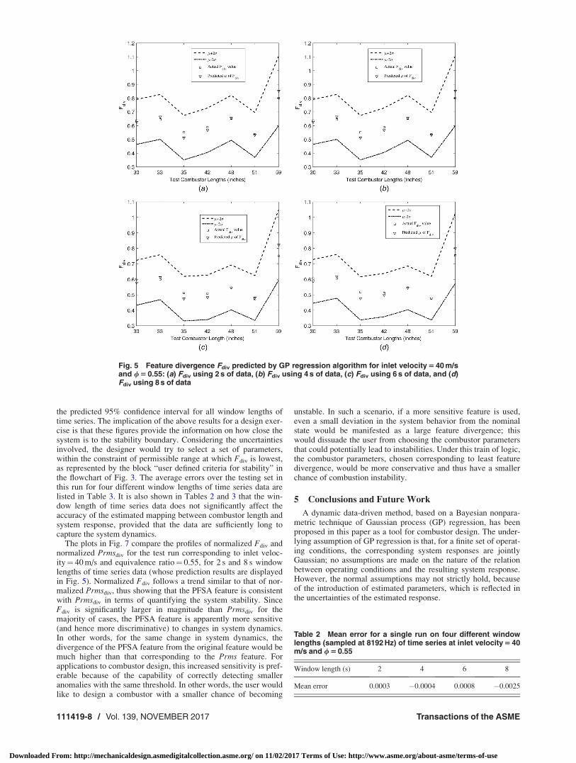
Figure 5 shows the mean (l) and the 95% confidence intervals(i.e., [l� 2r, lþ 2r) of Fdiv, predicted by the GP algorithm forall test cases, and the corresponding true values of Fdiv superim-posed on it, for a single run (i.e., a specific combination of trainingand testing data sets) for four different window lengths of timeseries: 2 s, 4 s, 6 s, and 8 s. The inlet velocity and equivalence ratiofor this subset are 40 m/s and 0.55, respectively. For this run, it isobserved that, for all test cases, the true value of Fdiv lies in thepredicted 95% confidence interval, for all four window lengths oftime series. In addition, for each widow length of time series, thedifference between predicted mean and true response value hasbeen noted for each test case, and the average is taken over all testcases in the testing set. The average errors over the testing set inthis run for the four different window lengths of time series dataare listed in Table 2.

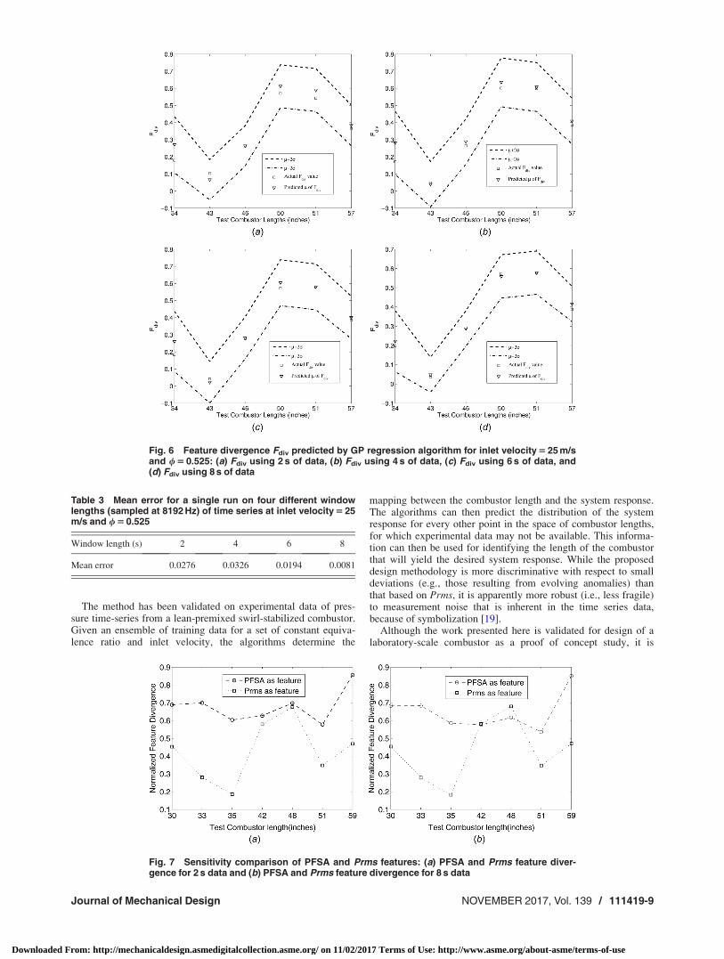
Figure 6 shows the mean (l) and the 95% confidence intervals(i.e., [l� 2r, lþ 2r]) of Fdiv, predicted by the GP algorithm forall test cases, and the corresponding true values of Fdiv superim-posed on it, for a single run (i.e., a specific combination of trainingand testing data sets) for four different window lengths of timeseries data (2 s, 4 s, 6 s, and 8 s), for another data set. The inletvelocity and equivalence ratio for this subset are 25 m/s and0.525, respectively. Similar to the results reported on the previoussubset, it is observed in this run that the true value of Fdiv lies in

Fig. 4 Effects of time series length on Prms profiles: (a) profileof Prms for a typical stable pressure signal and (b) profile ofPrms for a typical unstable pressure signal

Table 1 Classification accuracy for D-Markov machines (D 5 1)using SVM classifiers for different data lengths

Time series window length (s) 2 4 6 8

D-Markov parameters jRj ¼ 9 jRj ¼ 9 jRj ¼ 8 jRj ¼ 8Accuracy for linear kernel (%) 94 95 96 94Accuracy for radial basis functionKernel (r¼ 1) (%)

97 97 98 98

Journal of Mechanical Design NOVEMBER 2017, Vol. 139 / 111419-7

Downloaded From: http://mechanicaldesign.asmedigitalcollection.asme.org/ on 11/02/2017 Terms of Use: http://www.asme.org/about-asme/terms-of-use

the predicted 95% confidence interval for all window lengths oftime series. The implication of the above results for a design exer-cise is that these figures provide the information on how close thesystem is to the stability boundary. Considering the uncertaintiesinvolved, the designer would try to select a set of parameters,within the constraint of permissible range at which Fdiv is lowest,as represented by the block “user defined criteria for stability” inthe flowchart of Fig. 3. The average errors over the testing set inthis run for four different window lengths of time series data arelisted in Table 3. It is also shown in Tables 2 and 3 that the win-dow length of time series data does not significantly affect theaccuracy of the estimated mapping between combustor length andsystem response, provided that the data are sufficiently long tocapture the system dynamics.

The plots in Fig. 7 compare the profiles of normalized Fdiv andnormalized Prmsdiv for the test run corresponding to inlet veloc-ity¼ 40 m/s and equivalence ratio¼ 0.55, for 2 s and 8 s windowlengths of time series data (whose prediction results are displayedin Fig. 5). Normalized Fdiv follows a trend similar to that of nor-malized Prmsdiv, thus showing that the PFSA feature is consistentwith Prmsdiv in terms of quantifying the system stability. SinceFdiv is significantly larger in magnitude than Prmsdiv for themajority of cases, the PFSA feature is apparently more sensitive(and hence more discriminative) to changes in system dynamics.In other words, for the same change in system dynamics, thedivergence of the PFSA feature from the original feature would bemuch higher than that corresponding to the Prms feature. Forapplications to combustor design, this increased sensitivity is pref-erable because of the capability of correctly detecting smalleranomalies with the same threshold. In other words, the user wouldlike to design a combustor with a smaller chance of becoming

unstable. In such a scenario, if a more sensitive feature is used,even a small deviation in the system behavior from the nominalstate would be manifested as a large feature divergence; thiswould dissuade the user from choosing the combustor parametersthat could potentially lead to instabilities. Under this train of logic,the combustor parameters, chosen corresponding to least featuredivergence, would be more conservative and thus have a smallerchance of combustion instability.

5 Conclusions and Future Work

A dynamic data-driven method, based on a Bayesian nonpara-metric technique of Gaussian process (GP) regression, has beenproposed in this paper as a tool for combustor design. The under-lying assumption of GP regression is that, for a finite set of operat-ing conditions, the corresponding system responses are jointlyGaussian; no assumptions are made on the nature of the relationbetween operating conditions and the resulting system response.However, the normal assumptions may not strictly hold, becauseof the introduction of estimated parameters, which is reflected inthe uncertainties of the estimated response.

Fig. 5 Feature divergence Fdiv predicted by GP regression algorithm for inlet velocity 5 40 m/sand / 5 0.55: (a) Fdiv using 2 s of data, (b) Fdiv using 4 s of data, (c) Fdiv using 6 s of data, and (d)Fdiv using 8 s of data

Table 2 Mean error for a single run on four different windowlengths (sampled at 8192 Hz) of time series at inlet velocity 5 40m/s and / 5 0.55

Window length (s) 2 4 6 8

Mean error 0.0003 �0.0004 0.0008 �0.0025

111419-8 / Vol. 139, NOVEMBER 2017 Transactions of the ASME

Downloaded From: http://mechanicaldesign.asmedigitalcollection.asme.org/ on 11/02/2017 Terms of Use: http://www.asme.org/about-asme/terms-of-use

The method has been validated on experimental data of pres-sure time-series from a lean-premixed swirl-stabilized combustor.Given an ensemble of training data for a set of constant equiva-lence ratio and inlet velocity, the algorithms determine the

mapping between the combustor length and the system response.The algorithms can then predict the distribution of the systemresponse for every other point in the space of combustor lengths,for which experimental data may not be available. This informa-tion can then be used for identifying the length of the combustorthat will yield the desired system response. While the proposeddesign methodology is more discriminative with respect to smalldeviations (e.g., those resulting from evolving anomalies) thanthat based on Prms, it is apparently more robust (i.e., less fragile)to measurement noise that is inherent in the time series data,because of symbolization [19].

Although the work presented here is validated for design of alaboratory-scale combustor as a proof of concept study, it is

Fig. 6 Feature divergence Fdiv predicted by GP regression algorithm for inlet velocity 5 25 m/sand / 5 0.525: (a) Fdiv using 2 s of data, (b) Fdiv using 4 s of data, (c) Fdiv using 6 s of data, and(d) Fdiv using 8 s of data

Table 3 Mean error for a single run on four different windowlengths (sampled at 8192 Hz) of time series at inlet velocity 5 25m/s and / 5 0.525

Window length (s) 2 4 6 8

Mean error 0.0276 0.0326 0.0194 0.0081

Fig. 7 Sensitivity comparison of PFSA and Prms features: (a) PFSA and Prms feature diver-gence for 2 s data and (b) PFSA and Prms feature divergence for 8 s data

Journal of Mechanical Design NOVEMBER 2017, Vol. 139 / 111419-9

Downloaded From: http://mechanicaldesign.asmedigitalcollection.asme.org/ on 11/02/2017 Terms of Use: http://www.asme.org/about-asme/terms-of-use

envisioned that this method can be extended to more complexindustrial-scale combustors, because the input to this dynamicdata-driven approach is the pressure time series, which can be eas-ily generated in such combustors. In the initial stage of design, theactual experiments used to generate data in the present work maybe replaced by a limited number of high-fidelity simulations,involving unsteady Reynolds-averaged Navier–Stokes equation orlarge eddy simulations and state-of-the-art models for turbulentcombustion appropriate to the combustion mode at hand (e.g., pre-mixed, nonpremixed, or partially premixed). On the other hand,for modifications of existing combustors, knowledge acquiredfrom experiments can be used in the design. From these perspec-tives, topics of future research on the proposed design method aredelineated below.

(1) Theoretical and experimental research on how the proposeddynamic data-driven method can be gainfully integratedwith the current state-of-the-art (including the model-based) tools of combustor design.

(2) Performance comparison of the design algorithm withstate-of-the-art design methodologies not including usageof Prms.

(3) Evaluation of the design algorithm for different parameters(e.g., depth D> 1 instead of D¼ 1 (see Definition 4.4)).

(4) Testing of the design algorithm on combustors of differentgeometries and input parameters.

(5) Extension of the proposed methodology for design of com-bustors under active control.

Acknowledgment

The work reported in this paper has been supported in part bythe U.S. Air Force Office of Scientific Research (AFOSR) underGrant No. FA9550-15-1-0400. Any opinions, findings, and con-clusions or recommendations expressed in this publication arethose of the authors and do not necessarily reflect the views of thesponsoring agencies. The authors are thankful to ProfessorDomenic Santavicca at Pennsylvania State University, who hasprovided the experimental data.

References[1] Laera, D., 2015, “Nonlinear Combustion Instabilities Analysis of Azimuthal

Mode in Annular Chamber,” Energy Procedia, 82, pp. 921–928.[2] Lieuwen, T. C., and Yang, V., 2005, Combustion Instabilities in Gas Turbine

Engines: Operational Experience, Fundamental Mechanisms, and Modeling,American Institute of Aeronautics and Astronautics, Reston, VA.

[3] Lefebvre, A. H., 1999, Gas Turbine Combustion, 2nd ed., Taylor & Francis,Philadelphia, PA.

[4] Mattingly, J., Heiser, W., and Pratt, D., 2002, Aircraft Engine Design (AIAAEducation Series), 2nd ed., American Institute of Aeronautics and Astronautics,Reston, VA.

[5] O’Connor, J., Acharya, V., and Lieuwen, T., 2015, “Transverse CombustionInstabilities: Acoustic, Fluid Mechanic, and Flame Processes,” Prog. EnergyCombust. Sci., 49, pp. 1–39.

[6] Zahn, M., Schulze, M., Hirsch, C., and Sattelmayer, T., 2016, “Impact of Quar-ter Wave Tube Arrangement on Damping of Azimuthal Modes,” ASME PaperNo. GT2016-56450.

[7] Lei, L., Zhihui, G., Chengyu, Z., and Xiaofeng, S., 2010, “A Passive Method toControl Combustion Instabilities With Perforated Liner,” Chin. J. Aeronaut.,23(6), pp. 623–630.

[8] �Cosic, B., Bobusch, B. C., Moeck, J. P., and Paschereit, C. O., 2011, “Open-Loop Control of Combustion Instabilities and the Role of the Flame Responseto Two-Frequency Forcing,” ASME Paper No. GT2011-46503.

[9] Jones, C., Lee, J., and Santavicca, D., 1999, “Closed-Loop Active Control ofCombustion Instabilities Using Subharmonic Secondary Fuel Injection,” J. Propul.Power, 15(4), pp. 584–590.

[10] Paschereit, C. O., Gutmark, E. J., and Weisenstein, W., 1998, “Control of Ther-moacoustic Instabilities and Emissions in an Industrial Type Gas-TurbineCombustor,” Symp. Combust., 27(2), pp. 1817–1824.

[11] Bauerheim, M., Parmentier, J.-F., Salas, P., Nicoud, F., and Poinsot, T., 2014,“An Analytical Model for Azimuthal Thermo-Acoustic Modes in AnnularChamber Fed by an Annular Plenum,” Combust. Flame, 161(5), pp. 1374–1389.

[12] Bourgouin, J.-F., Durox, D., Moeck, J. P., Schuller, T., and Candel, S., 2015,“Characterization and Modeling of a Spinning Thermoacoustic Instability in anAnnular Combustor Equipped With Multiple Matrix Injectors,” ASME J. Eng.Gas Turbines Power, 137(2), p. 021503.

[13] Innocenti, A., Andreini, A., Facchini, B., and Cerutti, M., 2016, “NumericalAnalysis of the Dynamic Flame Response and Thermo-Acoustic Stability of aFull-Annular Lean Partially-Premixed Combustor,” ASME Paper No. GT2016-57182.

[14] Sarkar, S., Chakravarthy, S. R., Ramanan, V., and Ray, A., 2016,“Dynamic Data-Driven Prediction of Instability in a Swirl-StabilizedCombustor,” Int. J. Spray Combust. Dyn., 8(4), pp. 235–253.

[15] Sen, S., Sarkar, S., Chaudhari, R. R., Mukhopadhyay, A., and Ray, A., 2017,“Lean Blowout (LBO) Prediction Through Symbolic Time Series Analysis,”Combustion for Power Generation and Transportation: Technology, Chal-lenges and Prospects, A. K. Agarwal, S. De, A. Pandey, and A. P. Singh, eds.,Springer, Singapore, pp. 153–167.

[16] Darema, F., 2004, “Dynamic Data Driven Applications Systems: A New Para-digm for Application Simulations and Measurements,” International Confer-ence on Computational Science (ICCS), Krak�ow, Poland, June 6–9, pp.662–669.

[17] Daw, C., Finney, C., and Tracy, E., 2003, “A Review of Symbolic Analysis ofExperimental Data,” Rev. Sci. Instrum., 74(2), pp. 915–930.

[18] Hauser, M., Li, Y., Li, J., and Ray, A., 2016, “Real-Time Combustion StateIdentification Via Image Processing: A Dynamic Data-Driven Approach,”American Control Conference (ACC), Boston, MA, July 6–8, pp. 3316–3321.

[19] Beim Graben, P., 2001, “Estimating and Improving the Signal-to-Noise Ratioof Time Series by Symbolic Dynamics,” Phys. Rev. E, 64(5), p. 051104.

[20] Kim, K. T., Lee, J. G., Quay, B. D., and Santavicca, D. A., 2010, “Response ofPartially Premixed Flames to Acoustic Velocity and Equivalence RatioPerturbations,” Combust. Flame, 157(9), pp. 1731–1744.

[21] Sipser, M., 2012, Introduction to the Theory of Computation, Cengage Learn-ing, Boston, MA.

[22] Lind, D., and Marcus, B., 1995, An Introduction to Symbolic Dynamics andCoding, Cambridge University Press, Cambridge, UK.

[23] Ray, A., 2004, “Symbolic Dynamic Analysis of Complex Systems for AnomalyDetection,” Signal Process., 84(7), pp. 1115–1130.

[24] Mukherjee, K., and Ray, A., 2014, “State Splitting and Merging in ProbabilisticFinite State Automata for Signal Representation and Analysis,” Signal Process.,104, pp. 105–119.

[25] Bahrampour, S., Ray, A., Sarkar, S., Damarla, T., and Nasrabadi, N. M., 2013,“Performance Comparison of Feature Extraction Algorithms for Target Detec-tion and Classification,” Pattern Recognit. Lett., 34(16), pp. 2126–2134.

[26] Rajagopalan, V., and Ray, A., 2006, “Symbolic Time Series Analysis ViaWavelet-Based Partitioning,” Signal Process., 86(11), pp. 3309–3320.

[27] Vidal, E., Thollard, F., de la Higuera, C., Casacuberta, F., and Carrasco, R. C.,2005, “Probabilistic Finite-State Machines—Part I,” IEEE Trans. Pattern Anal.Mach. Intell., 27(7), pp. 1013–1025.

[28] Mallapragada, G., Ray, A., and Jin, X., 2012, “Symbolic Dynamic Filtering andLanguage Measure for Behavior Identification of Mobile Robots,” IEEE Trans.Sys. Man Cybern., Part B, 42(3), pp. 647–659.

[29] Rao, C., Ray, A., Sarkar, S., and Yasar, M., 2009, “Review and ComparativeEvaluation of Symbolic Dynamic Filtering for Detection of Anomaly Patterns,”Signal Image Video Process., 3(2), pp. 101–114.

[30] Bishop, C., 2006, Pattern Recognition and Machine Learning (Information Sci-ence and Statistics), Springer-Verlag, New York.

[31] Rasmussen, C., and Williams, C., 2005, Gaussian Processes for MachineLearning (Adaptive Computation and Machine Learning), MIT Press, Cam-bridge, MA.

[32] Cortes, C., and Vapnik, V., 1995, “Support-Vector Networks,” Mach. Learn.,20(3), pp. 273–297.

111419-10 / Vol. 139, NOVEMBER 2017 Transactions of the ASME

Downloaded From: http://mechanicaldesign.asmedigitalcollection.asme.org/ on 11/02/2017 Terms of Use: http://www.asme.org/about-asme/terms-of-use