Dynamic Simulation of a One Cylinder Engine Test...

IN THE FIELD OF TECHNOLOGYDEGREE PROJECT VEHICLE ENGINEERINGAND THE MAIN FIELD OF STUDYMECHANICAL ENGINEERING,SECOND CYCLE, 30 CREDITS

, STOCKHOLM SWEDEN 2017

Dynamic Simulation of a One Cylinder Engine Test RigImplementation of AVL Excite Designer for Durability Analysis of Power Transfer Components

PER CHRISTER SUNDSTRÖM

KTH ROYAL INSTITUTE OF TECHNOLOGYSCHOOL OF ENGINEERING SCIENCES

Dynamic Simulation of aOne-Cylinder Engine Test Rig

Implementation of AVL Excite Designer for Cardan Axleand Power Transfer Component Durability Analysis

Per Christer Sundstrom

A thesis presented as partial fulfilment for the degree ofMaster of Science in Engineering Mechanics

Department of Solid Mechanics

School of Engineering SciencesKTH Royal Institute of Technology

February 28, 2017

ABSTRACT

An engine test rig at AVL was redesigned with new components after afailure. The new system consists of a torsional vibration damper, a cardanaxle, a torque flange, and an adapter unit, together with a new dynamome-ter. To ensure another failure would not occur a study of the new systemwas conducted.

A general methodology for simulating the behaviour of a test rig powertrainwas developed using AVL Excite Designer and applied to the redesignedsystem. The simulated results were then used to evaluate the new compo-nents for durability. The loads obtained from AVL Excite were used for loadbased analysis, and used as boundary conditions in finite element models inAbaqus of components where load analysis was not su�cient.

Based on the results it was recommended that continuous operation at highloads in the RPM range below ⇡1650 is to be avoided to reduce the followingrisks:

• Overloading of the torsional vibration damper, which will result inexcessive wear of the unit shortening its life-span.

• Overloading of the torque flange, which can result in risk of fatiguefailure.

These results were e↵ects of an issue with excitation of a half-mode of thesystems eigenfrequency,

Possible alterations to shift the eigenfrequency of the system, and reduce theabove described issues, are increasing torsional compliance and/or increasingthe rotational inertia of certain components.

SAMMANFATTNING

En motortestrigg hos AVL har efter ett haveri blivit utrustad med nya kom-ponenter. Det nya systemet bestar av en, torsionssvangningsdampare, enkardan axel, en momentflans, och en adapterenhet, tillsammans med en nymotorbroms. For att forsakra sig om att ett nytt haveri inte skall intra↵autfordes en analys av det nya systemet.

En generell metod for att simulera beteendet hos drivlinan i en testriggutvecklades i AVL Excite Designer och tillampades sedan pa det nya sys-temet. Resultaten fran simuleringen anvande sedan for att utvardera hall-barheten hos de nya komponenterna. Belastningarna som beraknats i AVLExcite anvandes i belastningsbaserad analys, och som gransvarden i finitaelement modeller dar belastningsbaserad analys ej ansags tillracklig.

Baserat pa resultaten rekommenderades det att undvika korning av testriggenunder ⇡1650 RPM vid hog belastning da detta leder till risk for:

• Overbelastning av torsionssvangningsdamparen, vilket okar slitaget avkomponenten och forkortar dess livslangd.

• Overbelastning av momentflansen, vilket riskerar utmattningsbrott.

Dessa resultat var en e↵ekt av excitering av en halv-mod av systemets egen-frekvens.

Mojliga forandringar for att flytta denna egenfrekvens och minska dessaproblem ar att minska styvheten i systemet samt att oka troghetsmomentethos vissa komponenter.

ACKNOWLEDGEMENTS

I would like to extend my gratitude to Jonas Modin and Johannes Andersenat AVL who has given me the opportunity to do this thesis work as well asproviding supervision and support throughout the project.

I would also like to thank my supervisor at the Department of Solid Mechan-ics at KTH, Professor Soren Ostlund, for guidance, and Associate ProfessorArtem Kulachenko for giving valuable advice during the initial phase of theproject.

Finally, I would like to finish by thanking family and friends for supportand words of encouragement throughout my time at KTH Royal Instituteof Technology which comes to an end with the completion this thesis.

Per SundstromFebruary 28, 2017

CONTENTS

Abstract . . . . . . . . . . . . . . . . . . . . . . . . . . . . . . . . . . . i

Sammanfattning . . . . . . . . . . . . . . . . . . . . . . . . . . . . . . ii

Acknowledgements . . . . . . . . . . . . . . . . . . . . . . . . . . . . . iii

Contents . . . . . . . . . . . . . . . . . . . . . . . . . . . . . . . . . . iii

Notations . . . . . . . . . . . . . . . . . . . . . . . . . . . . . . . . . . vi

1. Introduction . . . . . . . . . . . . . . . . . . . . . . . . . . . . . . . 21.1 Problem . . . . . . . . . . . . . . . . . . . . . . . . . . . . . . 31.2 Objectives and Scope . . . . . . . . . . . . . . . . . . . . . . . 31.3 Limitations . . . . . . . . . . . . . . . . . . . . . . . . . . . . 3

2. Background and Theory of Methodology . . . . . . . . . . . . . . . 52.1 Test Rig Layout . . . . . . . . . . . . . . . . . . . . . . . . . 5

2.1.1 Component Specifics . . . . . . . . . . . . . . . . . . . 62.2 Failure Mechanics . . . . . . . . . . . . . . . . . . . . . . . . . 72.3 Solution Approach . . . . . . . . . . . . . . . . . . . . . . . . 82.4 AVL Excite Implementation . . . . . . . . . . . . . . . . . . . 9

2.4.1 Engine . . . . . . . . . . . . . . . . . . . . . . . . . . . 102.4.2 Torsional Vibration Coupling . . . . . . . . . . . . . . 152.4.3 Power Transfer Components . . . . . . . . . . . . . . . 162.4.4 Dynamometer . . . . . . . . . . . . . . . . . . . . . . . 162.4.5 Running Analysis . . . . . . . . . . . . . . . . . . . . . 16

2.5 Finite Element Analysis . . . . . . . . . . . . . . . . . . . . . 162.6 Validation of Models . . . . . . . . . . . . . . . . . . . . . . . 18

2.6.1 Torsion Model . . . . . . . . . . . . . . . . . . . . . . 182.6.2 Finite Element Models . . . . . . . . . . . . . . . . . . 19

3. Applied Methodology . . . . . . . . . . . . . . . . . . . . . . . . . 20

Contents v

3.1 Description of Installed System and Determination of Loads . 203.1.1 Engine . . . . . . . . . . . . . . . . . . . . . . . . . . . 203.1.2 Gearbox . . . . . . . . . . . . . . . . . . . . . . . . . . 213.1.3 Torsional Vibration Coupling . . . . . . . . . . . . . . 213.1.4 Cardan Axle . . . . . . . . . . . . . . . . . . . . . . . 223.1.5 Torque Flange and Adapter . . . . . . . . . . . . . . . 223.1.6 Dynanometer/Engine Brake . . . . . . . . . . . . . . . 22

3.2 Finite Element Model . . . . . . . . . . . . . . . . . . . . . . 233.3 Validation Procedures . . . . . . . . . . . . . . . . . . . . . . 263.4 Durability Analysis . . . . . . . . . . . . . . . . . . . . . . . . 27

4. Results . . . . . . . . . . . . . . . . . . . . . . . . . . . . . . . . . 294.1 Torsional System . . . . . . . . . . . . . . . . . . . . . . . . . 294.2 Durability Analysis . . . . . . . . . . . . . . . . . . . . . . . . 30

4.2.1 Load Based Analysis . . . . . . . . . . . . . . . . . . . 314.2.2 Finite Element Analysis . . . . . . . . . . . . . . . . . 314.2.3 Fatigue Analysis . . . . . . . . . . . . . . . . . . . . . 33

4.3 Parameter Study . . . . . . . . . . . . . . . . . . . . . . . . . 34

5. Discussion and Conclusions . . . . . . . . . . . . . . . . . . . . . . 38

6. Delimitations and Further Studies . . . . . . . . . . . . . . . . . . 40

References . . . . . . . . . . . . . . . . . . . . . . . . . . . . . . . . . . 40

Appendices . . . . . . . . . . . . . . . . . . . . . . . . . . . . . . . . . 43

NOTATIONS

Variables

F . . . . . . . . . . . . . . . Force [N]

r . . . . . . . . . . . . . . . Crank throw [m]

l . . . . . . . . . . . . . . . . Connecting rod length [m]

F

G

. . . . . . . . . . . . . . Force on piston caused by gas pressure [N]

F

S

. . . . . . . . . . . . . . Force from piston parallel to connecting rod [N]

F

N

. . . . . . . . . . . . . Force from piston on cylinder wall [N]

↵ . . . . . . . . . . . . . . . Crank angle [rad]

� . . . . . . . . . . . . . . . Connecting rod angle [rad]

F

T

. . . . . . . . . . . . . . Tangential force on crankshaft [N]

F

R

. . . . . . . . . . . . . . Radial force on crankshaft [N]

� . . . . . . . . . . . . . . . Crank throw over connecting rod length ratio [-]

x . . . . . . . . . . . . . . . Piston position [m]

x . . . . . . . . . . . . . . . Piston velocity [m/s]

x . . . . . . . . . . . . . . . Piston acceleration [m/s2]

m . . . . . . . . . . . . . . Mass [ kg ]

J . . . . . . . . . . . . . . . Mass moment of inertia [ kgm2]

a . . . . . . . . . . . . . . . Acceleration [m/s2]

. . . . . . . . . . . . . . . Damping ratio [-]

T . . . . . . . . . . . . . . . Torque [Nm]

Contents vii

W . . . . . . . . . . . . . . Polar moment of inertia [m4]

A . . . . . . . . . . . . . . . Area moment of inertia [m4]

Abbreviations

Dyno . . . . . . . . . . Dynamometer

RPM . . . . . . . . . . Revolutions Per Minute

FE . . . . . . . . . . . . . Finite Element

FEA . . . . . . . . . . . Finite Element Analysis

FEM . . . . . . . . . . . Finite Element Method

TDC . . . . . . . . . . . Top Dead Center

BDC . . . . . . . . . . . Bottom Dead Center

TVA . . . . . . . . . . . Torsional Vibration Analysis

TVS . . . . . . . . . . . Torsional Vibration System

TVD . . . . . . . . . . . Torsional Vibration Damper

DOF . . . . . . . . . . . Degrees of Freedom

MBS . . . . . . . . . . . Multi-Body Simulation

UTS . . . . . . . . . . . Ultimate Tensile Strength

PID . . . . . . . . . . . . Proportional-Integral-Derivative

SF . . . . . . . . . . . . . Safety Factor

1. INTRODUCTION

The purpose of this chapter is to serve as an introduction to the projectto describe in what context it exists as well as the specific problem that isaddressed.

The automotive engineering industry is under constant development in pur-suit of satisfying its customer’s needs as well as environmental requirementsfrom governing agencies. Due to strict regulations on emissions, powertraindevelopment has become a very important aspect when developing new ve-hicle platforms.

When developing combustion engines two separate fields of engineering,simulation and practical testing, are often utilized. While simulation hasbecome a very powerful and cost e↵ective tool when developing new con-cepts, companies still rely heavily on practical testing of the new conceptsto determine their validity in terms of proof of concept, functionality, anddurability.

Companies developing powertrains often do this by having test rigs wherea conceptual or fully developed engine can be tested for di↵erent settingsand loads while accurately measuring parameters of interest such as torque,power, emissions, fuel consumption, etc. simultaneously. These systems willdi↵er depending on what function the rig is supposed to serve. Generally,the setup of a system like this consists of the engine under developmentconnected to a dynamometer or dyno, which absorbs the engines poweroutput.

The test rig treated in this thesis consists of a one-cylinder natural gasengine, used for testing di↵erent combustion parameters for engines underdevelopment. The use of only one-cylinder makes it easier to monitor andrecord parameters specific to the processes of combustion and emissions,which in a multi-cylinder engine would be harder to distinguish in between.This because these parameters directly relate to each individual combustioncycle taking place in every cylinder for each stroke.

1. Introduction 3

1.1 Problem

The thesis project concluded by this report was conducted at AVL MTCAB in Sodertalje, where a test rig as described in the previous section hadsu↵ered a critical failure of its connection between the dyno and engine. Theengine was connected through a gearbox to a dyno by two cardan axles, ofwhich one failed, breaking the dyno as well as the gearbox housing.

To get the rig operational again a new dyno, as well as a new connectionbetween the dyno and engine was ordered. To avoid another critical failureAVL decided that a durability analysis was to be conducted on the newsystem connecting the dyno and engine.

1.2 Objectives and Scope

The purpose of the work conducted was to simulate the behaviour of thesystem with the new connection in place and to conduct durability analysison the new components. This was to result in finding the operational condi-tions under which the system will perform well and find possible limitationsof the new system that could be an issue under normal operation. Finally,this was to result in operational instructions and limitations to prevent an-other critical failure from occurring.

The expected contributions from this study were several, the main one beingensuring the durability of the new system design. It was also desired by AVLthat the software AVL Excite was to be used for the analysis of the system.The purpose of this was to increase knowledge of its possibilities as well asserving as a platform for further development of a model, which can be usedfor a variety of durability and vibration related simulations.

1.3 Limitations

Work presented in this thesis was based on studying the torsional vibra-tions and durability of the new powertrain components. The engine wasnot considered a part of this system. Therefore, no durability analysis orstudies were performed on the internal components of the engine, such asthe connecting rod and crankshaft, other than the analysis necessary forsatisfactory results in the analysis of the powertrain components.

1. Introduction 4

Due to some information treated in this thesis being under Non-DisclosureAgreement, certain parameters were unavailable or left out. These parame-ters have been estimated using outside sources and engineering judgement,and will for most cases be available if the developed method is to be usedon other systems.

2. BACKGROUND AND THEORY OF METHODOLOGY

The information presented in this chapter was condensed from a literaturestudy and intends to create a fundamental understanding of systems like theone treated as well as the mechanics of the failure observed, and describe ageneral approach to conduct the requested analysis.

2.1 Test Rig Layout

Test rigs are used in many stages of the process of developing new engines,and there is a multitude of di↵erent systems with di↵erent purposes due tothe advantages that the use of test rigs gives. When conducting tests theoperator has complete control of all external parameters which in the realworld would be varying, such as air temperature, load. etc. Additionally,the operation can be made completely automatic, meaning that long termtransient tests for durability can be conducted. The use of these systemsalso allow for close monitoring and measurement of many output parametersthat during normal operating conditions are not easily measurable, some-times not at all, and sometimes not with the same accuracy. Examples ofsuch parameters are exhaust emissions, which however are becoming moremeasurable with portable devices.

A test rig can simply be divided into three subsystems, a combustion engine,a dynamometer or dyno, usually consisting of an electric motor breaking theengine during testing, and a power transfer system usually consisting of adrive axle, connecting the two. Each of these subsystems will consist ofseveral components. In addition to this several sensor units will monitorcertain parameters of the system. A basic schematic can be seen in Figure2.1.

2. Background and Theory of Methodology 6

Fig. 2.1: Schematic test rig layout

2.1.1 Component Specifics

The most vital component of the power transfer system is usually an axle,with the main purpose of transferring the rotational motion of the engineto the dyno. Several di↵erent axle systems exist, all with di↵erent charac-teristics depending on the application. One thing that often needs to beaccounted for is relative motion between the engine and dyno. This kindof motion is common in automotive related applications, and can not berestricted by the drive axle. To allow for this kind of motion most axleshave a spline section allowing for axial movement and two joints allowing itto bend while rotating. The most common version of these joints are eitherconstant velocity (CV) or cardan/universal joints.

Fig. 2.2: Cardan/universal joint [1]


The main di↵erence between the two joints is how the rotational velocityis a↵ected by the joint. The geometry in a universal joint will create avariation in the rotational velocity whilst the CV joint will as the namesuggests maintain constant velocity, at the cost of complexity, price, andweight. A cardan joint can be seen in Figure 2.2.

To reduce the impulse e↵ect of the torque delivery from reciprocating en-gines, torsional vibration dampers can be used. The purpose of this compo-nent is to allow for torsional flexibility in the system between engine/flywheeland axle, which reduces the above described e↵ect. These are commonlyrubber components, a material with properties that allow for large displace-ments without permanent deformation.

To monitor the torque output, a component known as a torque flange canbe used, which utilizes string gauge technology This methods relies on de-formation of the component to calculate the the torque it transfers.

Sometimes adapter plates of di↵erent kinds are needed to connect the abovementioned components. This can be avoided by sticking to a standard con-nection, such as DIN or SAE, which both exist in several sizes for di↵erentkinds of components. This is not always a possibility, and in these instancesadapters between the two di↵erent components can be used.

Lastly, there is a dyno, with the purpose of absorbing the power output ofthe engine. In older systems other methods of absorbing the engines powerhave been utilized, such as adjustable resistance water pumps, but mostmodern dyno systems consist of an electric motor working as a generator tobrake the engine.

2.2 Failure Mechanics

When it comes to the durability of machine elements, fatigue is the numberone cause of failure. Up to 80 % of all failures can be attributed to fatigueand is therefore a phenomenon that can not be overseen in rotating andvibrating systems [2].

Fatigue is when a component fails or is damaged from repeated loadingand unloading at stress levels significantly lower than the materials yield-and ultimate strength. It can be seen as a wear of the material properties,resulting in phenomena such as micro cracks and other anomalies that couldresult in failure.


When discussing fatigue, it is often divided into two di↵erent mechanisms,high and low cycle fatigue. Low cycle fatigue results in failure after only afew load cycles and can be for example observed when bending a nail backand forth. High cycle fatigue is a more common issue in machine elementswhere loads are not near the maximum load capability, but where vibrationand variation of loads exist.

The mechanism behind fatigue is dependent on load history, and can forcomplex load scenarios become di�cult to describe accurately. In manycases it is deemed necessary to get an accurate estimate of the fatigue prop-erties. One example of this is in airplanes, where it is important that partsdo not brake mid-flight. A more simplistic approach is to assume a worstcase load scenario and determine the durability if loaded continuously likethis. This will give an underestimate of the fatigue durability, ensuring thatfailure will not occur before what is predicted.

Fatigue failure is especially common in systems containing reciprocating ma-chinery as a result of the cyclic loading introduced by the working principleof such machines, which also introduces the possibility of resonance [3]. Fa-tigue is also a common issue in cardan axles operating at large angles whichcause large fluctuations in rotational velocity of the axle, introducing cyclicloading. For axles operating at small angles, this issue is diminished, butthe issue connected with reciprocating engines still exist. Points that com-monly fail are the yokes and cross (see Figure 2.2) of the universal joints ina cardan axle, as well as the tube section [3]. These points are therefore ofspecific interest when conducting the present type of analysis.

Another mode of failure that must be considered for rotating systems in-volving long axles is the axles critical bending speed. When the rotationspeed of an axle reaches this limit it will begin to resonate, causing largevibrations and possibility of axle failure [4].

2.3 Solution Approach

When designing systems containing reciprocating machinery, the generalapproach is to conduct torsional vibration analysis to avoid issues like theones described in the previous section [5].

This serves as a first step in the process of determining the durability ofa powertrain, with the purpose of identifing the mode of operation thatwill yield the highest load on the system. This is the critical load that


the system must be able to endure under an extended period of time toavoid issues with fatigue. For most powertrains the largest torsional loadwill result from high load operation at certain RPM/frequencies [6] and theanalysis must therefore be conducted over a range of engine speeds.

When conducting torsional vibration analysis a common approach is to uti-lize modal analysis [6], as this is a time e↵ective method that does not requirefull explicit analysis while still giving the frequency response of transientloadings. This method does however come with the limitation of assum-ing linear behaviour of all components for a set frequency, meaning thatmodelling of complex behaviours are limited.

The software AVL Excite Designer consists of a module that utilizes thismethod for calculation of loads on engine and powertrain components. Thismethod will determine the dynamic response of the system under transientloading from the engine.

This response analysis will for some components be su�cient to determinetheir durability, as they have well defined specifications given from the manu-facturer on what loads they are built to sustain. For other components,further analysis will have to be conducted to determine their durability. Forthese components the loads will serve as boundary conditions in a model forfinite element analysis, to determine local stresses and subsequently the riskof failure.

These FE models also serve as a good base for determining the criticalbending speed of axles, where the first bending frequency multiplied with60 gives the critical bending speed in RPM.

2.4 AVL Excite Implementation

AVL Excite consists of several modules with di↵erent purposes, such assimulation of bearings, camshaft synchronization, NVH analysis, etcetera.Excite Designer can be seen as an analytical multi body simulation tool usedto determine boundary conditions for durability analysis of drivetrain com-ponents. AVL Excite Designer models the system as a mass-spring system,where each component is divided into and represented by inertia points andelements with torsional sti↵ness. It then calculates the eigenfrequencies andeigenmodes as well as the frequency response from the transient loading ofthe engine.


2.4.1 Engine

Excite begins by calculating the torque output from the engine. The work-ing principle for reciprocating engines relies on the burning of combustibleliquids or gases [7]. A mixture of oxygen and a flammable fuel such as gaso-line or diesel is injected into the combustion chamber. When the mixture iscompressed and then ignited, the combustion will cause the gases to expand,pushing the piston down. This process consisting of four cycles can be seenin Figure 2.3. A geometrical system consisting of a connecting rod and acamshaft will then convert this transversal piston motion to a rotationalmotion that can be used to drive the vehicle forward.

Fig. 2.3: Working principle of a four stroke engine [8]

The torque profile of the engine will be the result of certain processes in theengine, mainly the gas forces created by the combustion cycle and the massforces as a result of velocity changes in components with mass, such as thepiston [7].

Gas Forces

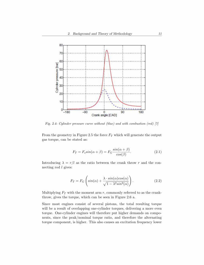
To calculate the torque generated by the gas forces the geometry of themechanical system created by the piston, crankshaft, and the connecting rodmust be considered. Initially the combustion process will create a pressureon the piston. A cylinder pressure curve for one-cylinder can be seen inFigure 2.4. The pressure shown will push down on the piston causing alateral force F

G

, which by the geometry of the crankshaft will cause it torotate.


Fig. 2.4: Cylinder pressure curve without (blue) and with combustion (red) [7]

From the geometry in Figure 2.5 the force FT

which will generate the outputgas torque, can be stated as:

F

T

= F

s

sin(↵+ �) = F

G

sin(↵+ �)

cos(�). (2.1)

Introducing � = r/l as the ratio between the crank throw r and the con-necting rod l gives:

F

T

= F

G

sin(↵) +

� · sin(↵)cos(↵)p1� �

2sin

2(↵)

!. (2.2)

Multiplying F

T

with the moment arm r, commonly referred to as the crank-throw, gives the torque, which can be seen in Figure 2.6 a.

Since most engines consist of several pistons, the total resulting torquewill be a result of overlapping one-cylinder torques, delivering a more eventorque. One-cylinder engines will therefore put higher demands on compo-nents, since the peak/nominal torque ratio, and therefore the alternatingtorque component, is higher. This also causes an excitation frequency lower


Fig. 2.5: Forces on the crank mechanism [7]

than that in multi-cylinder engines as well as high impact drive under heavyload. One-cylinder engines therefore have a load scenario more demandingthan most engines, increasing the risk of a failure that normally would notoccur in multi-cylinder systems.

Fig. 2.6: Alternating (blue) and nominal (red) for a one (left) and an inline four(right) cylinder engine [7]

Equation (2.2) is together with the definition of a pressure curve and thecomponent geometry used in Excite to calculate the gas forces of the en-gine.


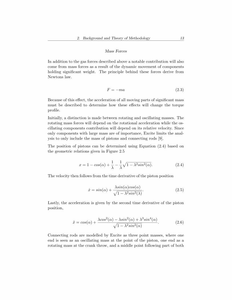
Mass Forces

In addition to the gas forces described above a notable contribution will alsocome from mass forces as a result of the dynamic movement of componentsholding significant weight. The principle behind these forces derive fromNewtons law.

F = �ma (2.3)

Because of this e↵ect, the acceleration of all moving parts of significant massmust be described to determine how these e↵ects will change the torqueprofile.

Initially, a distinction is made between rotating and oscillating masses. Therotating mass forces will depend on the rotational acceleration while the os-cillating components contribution will depend on its relative velocity. Sinceonly components with large mass are of importance, Excite limits the anal-ysis to only include the mass of pistons and connecting rods [9].

The position of pistons can be determined using Equation (2.4) based onthe geometric relations given in Figure 2.5

x = 1� cos(↵) +1

�

� 1

�

p1� �

2sin

2(↵). (2.4)

The velocity then follows from the time derivative of the piston position

x = sin(↵) +�sin(↵)cos(↵)p1� �

2sin

2(�). (2.5)

Lastly, the acceleration is given by the second time derivative of the pistonposition,

x = cos(↵) +�cos

2(↵)� �sin

2(↵) + �

3sin

4(↵)p1� �

2sin

2(↵). (2.6)

Connecting rods are modelled by Excite as three point masses, where oneend is seen as an oscillating mass at the point of the piston, one end as arotating mass at the crank throw, and a middle point following part of both


motions. Crankshaft counter weights are also modelled as rotating masses,with acceleration according to the following equation:

x

rot

= r!

2. (2.7)

where ! is the rotational velocity given by the engines RPM. These accelera-tions are multiplied with the mass of each respective component to calculatethe mass forces, and then by the torque arm to give the mass torque.

Crankshaft Flexibility

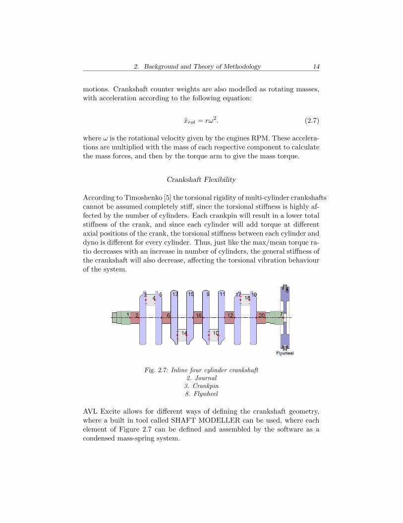
According to Timoshenko [5] the torsional rigidity of multi-cylinder crankshaftscannot be assumed completely sti↵, since the torsional sti↵ness is highly af-fected by the number of cylinders. Each crankpin will result in a lower totalsti↵ness of the crank, and since each cylinder will add torque at di↵erentaxial positions of the crank, the torsional sti↵ness between each cylinder anddyno is di↵erent for every cylinder. Thus, just like the max/mean torque ra-tio decreases with an increase in number of cylinders, the general sti↵ness ofthe crankshaft will also decrease, a↵ecting the torsional vibration behaviourof the system.

Fig. 2.7: Inline four cylinder crankshaft2. Journal3. Crankpin8. Flywheel

AVL Excite allows for di↵erent ways of defining the crankshaft geometry,where a built in tool called SHAFT MODELLER can be used, where eachelement of Figure 2.7 can be defined and assembled by the software as acondensed mass-spring system.


The inertia of bearing journals is calculated by putting measurements of di-ameters and lengths of each segment into the SHAFT MODELLER module.The sti↵ness of these elements is calculated by the program using Euler-Bernoulli beam theory [9]. The sti↵ness of the more complex geometries,mainly the crankpins, can be calculated in several ways. Timoshenko o↵ersseveral ways of estimating the sti↵ness of crankpins [5] but a Finite Ele-ment approach can also be utilized. When defining the sti↵ness in Excite,half of the bearing journal on each side of the crankpin is included in theanalysis, since this is where the inertia points are placed in the mass-springsystem.

Fig. 2.8: Condensed mass-spring crankshaft

2.4.2 Torsional Vibration Coupling

When modelling a torsional vibration damper in Excite, two main prop-erties must be accounted for, elasticity and damping of the component,respectively.

Defining fully accurate material models of rubber is a di�cult task whichoften results in highly complex and computationally time-consuming mod-els. Several methods of modelling damping exist [10], which all describedi↵erent kind of damping behaviour more or less accurately. However, whenmodelling rubber in systems like this one it is not a case of getting a per-fect dynamic representation of the material, which in this case would bevery hard since modal analysis relies on linear behaviour. Instead, one mustremember the limitations of the model and what this can result in.

Excite Designer o↵ers two ways of modelling the damping characteristics.The damping coe�cient v with units [Nms/rad] is velocity dependent, andthe damping ratio describes how much of the vibration energy that isabsorbed by the damper and converted into heat. The torsional sti↵ness ofthe damper can simply be defined as a value in [Nm/rad].


2.4.3 Power Transfer Components

All components in the path between the engine and dyno can be seen aspower transfer components as they all must be able to deal with the torquethe engine delivers. The number of components as well as their purpose canvary greatly depending on the system, and will all be a↵ecting the dynamicbehaviour of the assembled system. Here the system must be divided intoparts of inertia and sti↵ness defined as [kg/m2] and [Nm/rad], where gearratios from components like gearboxes also can be defined.

2.4.4 Dynamometer

Similarly to the power transfer components, the characteristic of the dynothat is important to have represented in the simulation software is theinertia, which just like for the power transfer components is defined in[kg/m2].

2.4.5 Running Analysis

When the entire system is defined in AVL Excite, the analysis can be runfor a range of RPM values which will calculate the forces each componentis subjected to under that mode of operation.

For many components this will be su�cient to determine the durability ofa component, as many products come with data sheets from the manufac-turer with information on what type of load the component is designed toendure.

2.5 Finite Element Analysis

While the durability of some components can be determined using datasheets from the manufacturer, some components will require further analy-sis to determine their durability. These are most commonly new designedcomponents or one-o↵ components designed for only one type of application.For these components, Finite Element Analysis can be used to determinetheir durability.


FEA is an approximative method which relies heavily on computer inten-sive calculations. The theory behind the method is to take a geometricallycomplex part and subdivide it into a mesh of small finite elements, wheresimple algebraic equations describe the behaviour of each element. Theseequations can be assembled to form a system of equations that can be solvedto describe the behaviour of the entire structure.

To reduce the time needed for computing the goal is always to have a modelthat is as simple as possible without losing accuracy. Added complexity interms of increased number of elements comes at the cost of simulation time,but will not always yield more accurate results. This is because the addedelements can be in areas where high resolution is not needed. Thereforeit is preferable to stepwise increase mesh resolution until a stabilization ofthe results is observed. This ensures that elements that do not improve theaccuracy of the results are not added unnecessarily.

When applying FE methodology on durability analysis of geometrically com-plex components, it is important that the virtual geometry used representsthe components well, as minor geometric di↵erences can cause large de-viances in the calculated stresses and strains. When conducting this typeof durability analysis the FE models are used to calculate the stresses andstrains in the geometry resulting from the boundary conditions calculatedby the AVL Excite MBS analysis. These stress values are then used for thefatigue analysis.

Good practice is to use the following rules:

Ensure good mesh quality: Low quality meshes will give unreliable re-sults.

Avoid excessive mesh refinement: A highly refined mesh will yield moreaccurate results. FE analysis is however a computer intensive task and itis therefore good practice to keep the model as simple as possible. Meshconvergence studies are often utilized to ensure this, where the element sizein areas of importance is successively decreased until consistent results areobserved.

Remove unnecessary complexity: Many components have features thatadd to the complexity of the meshed part. Examples of this can be sweptsurfaces, fillets, and holes. However, it must be noted that these features cannot always be removed. One must practice caution as to where these featurescan be considered not to a↵ect the final results. For example, the stress inan internal corner will be significantly a↵ected by the radii in the corner,


and can therefore not be removed. Other ways of simplifying FE models isto make use of shell elements when applicable, such as tubular segments ina cardan axle, as these are less computationally demanding.

To determine the first bending frequency for the critical bending speed, thedensity of elements must be defined, as this frequency is a↵ected by themass/sti↵ness ratio. This frequency is calculated using frequency analy-sis in Abaqus [11], where the first bending eigenfrequency can be deter-mined.

2.6 Validation of Models

When analysing complex systems it is always of good measure to start bysimplifying the system and studying the behaviour of the simplified version.This is done to determine if the results obtained are reasonable or not, sincethe results of a simple model is easier to derive from basic analytical theory.Complexity can then be added, and the results from the simplified modelcompared to the full model.

2.6.1 Torsion Model

A simplified analysis of a torsional vibration system is to find the eigenfre-quency of the first torsional mode. The process of simplifying the systemis done by condensing several components and modelling them as one, untilyou reach a point where the system can be analysed using basic theory. Thisprinciple is explained in Figure 2.9.

By identifying the most torsionally compliant component and condensingthe system around this point as a spring and two point masses with inertia,a simple system is defined. The first eigenmode will twist about this spring,and the frequency for this mode can be calculated. For most systems themost torsionally compliant component will be the torsional vibration cou-pling. To calculate the frequency the combined inertia on each side of thetorsional spring J1 and J2 as well as the spring sti↵ness K are used inEquation (2.8) [12]

f =1

2⇡

s(J1 + J2)K

J1J2. (2.8)


Fig. 2.9: Condensed torsional vibration model

This value can be compared to the first eigenmode calculated by Excite,which should be of similar magnitude.

2.6.2 Finite Element Models

Validation procedures will also have to be applied to the FE models usedin the analysis. These will however have di↵erent approaches depending onthe geometry of the part, and a general method can not be described. Forexample, many geometries can be simplified as generic beams and analysedusing Euler-Bernoulli beam theory. The results are preferred to be of thesame order of magnitude, but not necessarily identical.

3. APPLIED METHODOLOGY

The purpose of this chapter is to describe the exact methodology applied tothe system analysed at AVL. This means a more in-depth description of thesystem as a whole, as well as the specific methods used.

3.1 Description of Installed System and Determination of Loads

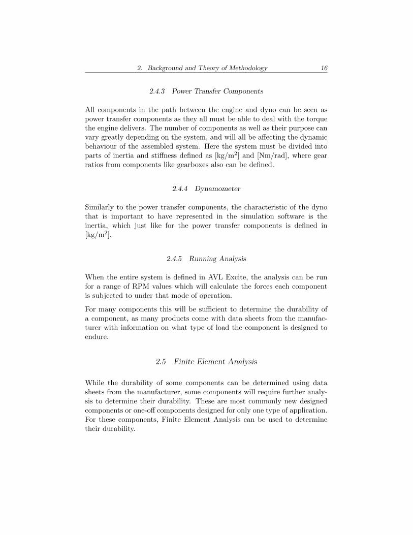
To determine the loads on each of the components in the system, themethodology described in the Chapter 2 was applied to the considered sys-tem. The torques transferred by each component was calculated using AVLExcite Designer, and used in the FE and durability analyses. The system isseen in Figure 3.1.

Fig. 3.1: Graphical schematic of AVL Excite Designer system

3.1.1 Engine

The engine installed in the rig at AVL is a one-cylinder natural-gas en-gine. This means that the issues described in Chapter 2 regarding a highpeak-nominal ratio will be present combined with a low excitation fre-quency.

Cylinder pressure data was imported into AVL Excite Designer, togetherwith the mass of the piston and the connecting rod. The crankshaft was

3. Applied Methodology 21

modelled using SHAFT MODELLER, where the sti↵ness of the crankpinswas determined using FE methodology.

3.1.2 Gearbox

The dyno mounted in the previous system had a maximum torque of 100 Nm,meaning that it could not deliver enough brake torque if connected directlyto the engine. It was therefore connected to a 1:4 ratio gearbox decreasingthe necessary peak RPM from the motor to the dyno. For the new systema stronger motor is used, and therefore a gearbox is not needed.

3.1.3 Torsional Vibration Coupling

The torsional vibration coupling used in the simulated system consists oftwo discs axially and radially connected to each other, along with a rubberring element between the two to transfer the torque (Figure 3.2).

Fig. 3.2: Stromag TVD [13]

Due to Excite Designers limitations of only utilizing linear theory for analysisof the dynamic behaviour, a fairly simple model was used to model this


component. The bahaviour of the coupling is from the manufacturer givenat a certain dynamic loading sequence. The elasticity is simply given asthe torsional sti↵ness, while the damping is given as the damping ratio described in Chapter 2 [13].

For the damping behaviour of rubber at low frequencies <200 Hz a decreasein damping is not expected [10]. This combined with the assumption thatthe amplitude dependence of the rubber damping can be neglected, resultedin a model requiring only the torsional sti↵ness, damping ratio, and inertiaof the two connected discs as input.

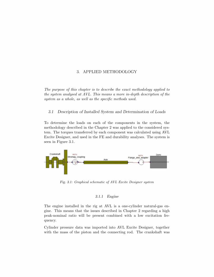
3.1.4 Cardan Axle

The data needed to set up a model as described in the previous chapter arethe inertia and sti↵ness properties of the axle. These are given in the datasheet of the installed axle [14].

Fig. 3.3: CAD drawing of cardan axle

3.1.5 Torque Flange and Adapter

The output axle of the dyno was connected to the torque flange using anadapter designed by AVL for the specific purpose. Since it was vital thatthe sti↵ness and inertia of all components in the system were present in themodel, these components were included. While the inertia and sti↵ness ofthe torque flange was available from the manufacturer [15], the adapter iner-tia was determined in the CAD software, and the sti↵ness using FEM.

3.1.6 Dynanometer/Engine Brake

Since the old dyno was damaged at the failure of the previous system anew dyno was ordered. The new motor is a Leroy Somer LSK 1604 C VL13brushless D.C. motor with a power rating of 130 kW and a maximum RPM of


Fig. 3.4: Adapter between torque flange and dyno

4000 capable of delivering a torque of 503 Nm [16]. The velocity and torqueof this type of motor is controlled through a PID controller using electroniccommutation to regulate the electric field surrounding the rotor.

The main contributor to the dynamic behaviour of the system from thedyno is its rotational inertia, listed at 0.64 kgm2, and the torque it developsto resist the torque of the engine, which maintains a constant rotationalvelocity of the system.

With a mean torque output from the engine just below 400 Nm at fullload, the dyno will output the same torque to maintain a constant speed.While complex ways of modelling dynos exist in the AVL Excite Power Unitmodule, Excite Designer only allows for simple mass/inertia modelling of thedyno. This is, however, a reasonable assumption considering the responsetime of the motor combined with the use of a PID controller with the purposeof trying to maintain a constant torque.

3.2 Finite Element Model

When developing finite element models of components it is vital that the ge-ometry used is accurately representing the physical parts. Since the adapterunit connecting the dyno to the torque flange is a component designed byAVL, an accurate description of the geometry of this component was avail-able. However, no accurate CAD geometry of the cardan axle existed, so thiscomponent was drafted based on physical measurements of the component.It is important to note that this is not the preferred method for obtainingthis type of data, and caution must be practised to make measurements as


accurate as possible. The axle geometry in Figure 3.3 was drafted in CatiaV5.

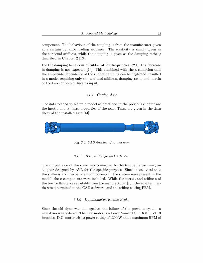
The components were then imported into the commercial FEM softwareAbaqus. To simplify the analysis, bearings and bearing cups were not anal-ysed to remove contact conditions. Separate models for each component wasinstead created. However, this required more complex modelling of the dis-tributed pressure created by the bearing in the cardan joint. The pressuredistribution had to represent how bearings distribute loads across the bear-ing surface. By creating a local coordinate system at each bearing center,the distribution described in Equation (3.1) was used to create the pres-sure distribution seen in Figure 3.5, a common approach when modellingbearings [17].

Pcos

2⇡X

2di

= F

r

(3.1)

Fig. 3.5: Bearing pressure distribution [17]

When meshing the components the seed size and consequently the numberof elements was increased until the results obtained were similar as for theprevious seed size. Since computation times at su�cient seed size was short,there was no need for local mesh refinements other than at the radii at theend of the bearing surface of the cardan cross.


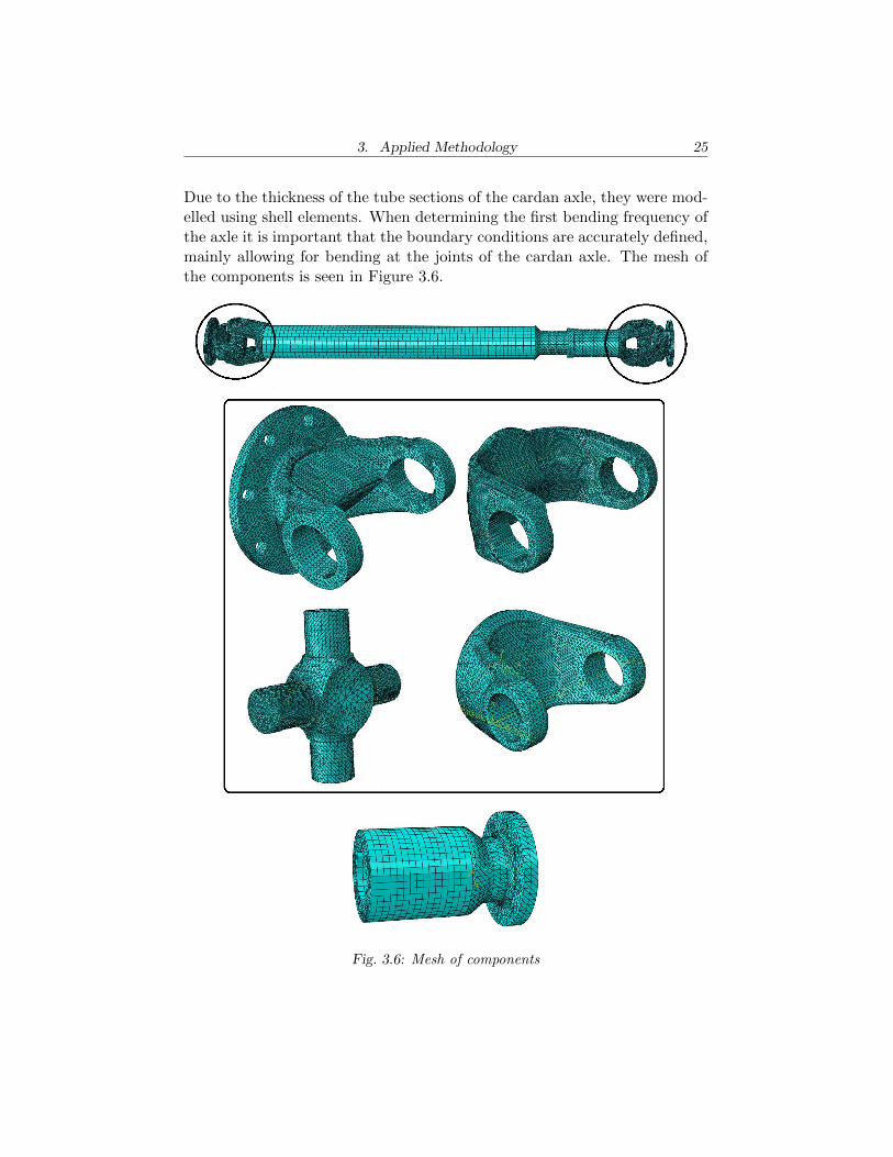
Due to the thickness of the tube sections of the cardan axle, they were mod-elled using shell elements. When determining the first bending frequency ofthe axle it is important that the boundary conditions are accurately defined,mainly allowing for bending at the joints of the cardan axle. The mesh ofthe components is seen in Figure 3.6.

Fig. 3.6: Mesh of components


3.3 Validation Procedures

The torsion model determined in AVL Excite was compared to the valueof the first eigenfrequency calculated using the methodology described inChapter 2 and Figure 2.9. Since the TVD was the most torsionally compliantcomponent, the inertia for the components on each side of the damper werelumped together.

To verify the results obtained from the FEA, the geometry of each modelwas simplified as basic shapes such as circular or rectangular beams, whereEuler-Bernoulli beam theory for standard load cases is applicable. The sameprinciple was used for the adapter component.

The tube section of the cardan axle was simplified as circular beams intorsion, where an estimate of the maximum normal stress could be estimatedusing Equation (3.2) where W is the torsion constant of the tube [18].

�

max

=p3⌧

max

=p3T

W

r (3.2)

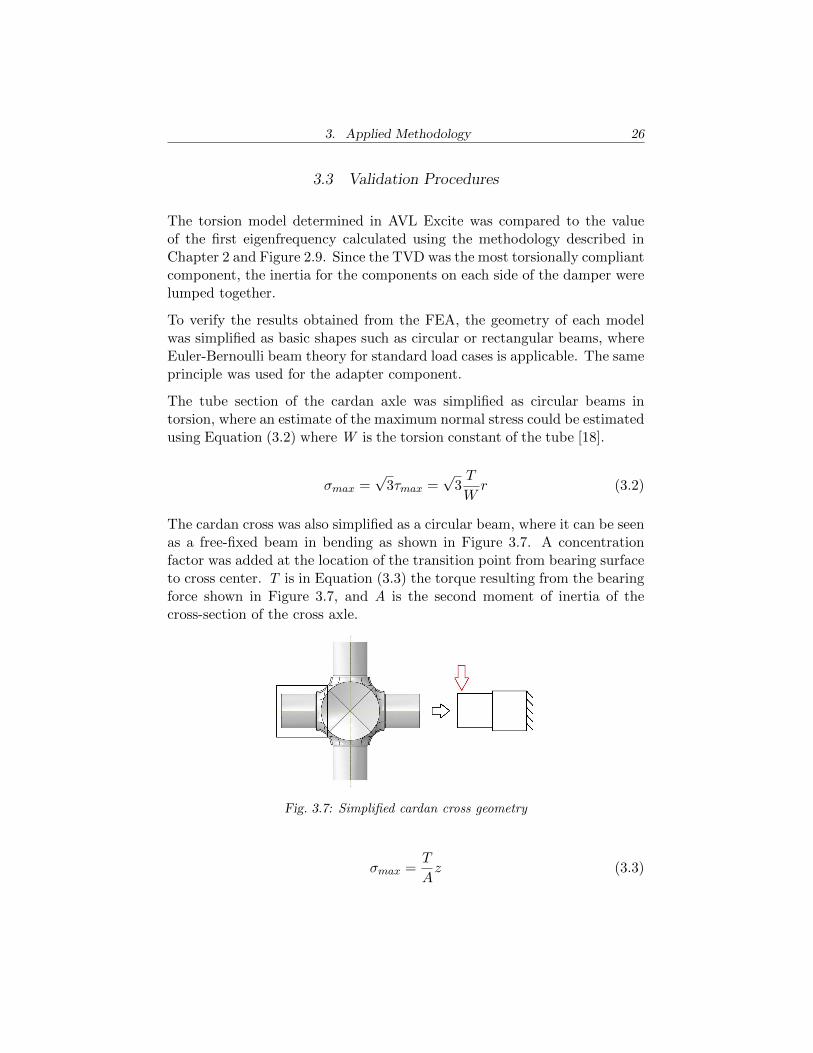
The cardan cross was also simplified as a circular beam, where it can be seenas a free-fixed beam in bending as shown in Figure 3.7. A concentrationfactor was added at the location of the transition point from bearing surfaceto cross center. T is in Equation (3.3) the torque resulting from the bearingforce shown in Figure 3.7, and A is the second moment of inertia of thecross-section of the cross axle.

Fig. 3.7: Simplified cardan cross geometry

�

max

=T

A

z (3.3)


The validation of the yoke components required major geometry simplifica-tions to be made. Each yoke arm was simplified as a fixed-free beam loadedin bending, yet again using Equation (3.3) for an estimate of the stress.Due to the simplifications made, a bigger di↵erence can be expected here.Furthermore, this method does not calculate the stress at its maximum lo-cation, and engineering judgement will have to be used to determine theplausibility of local stress concentrations.

3.4 Durability Analysis

As mentioned in Chapter 2, failure of machine elements is commonly due tofatigue, and must therefore be accounted for. For the TVD and the torqueflange, load magnitudes resulting in a durability risk are listed in data sheets[13, 15], making this analysis simple.

Such values does not exist for the adapter component, and the results fromthe FEA had to be used for a durability estimation. Although some dura-bility data for the cardan axle exists, the equations used for calculation ofthese values indicate unreliability when the component is subjected to thevarying load created by a one-cylinder engine, and a full FEA was thereforeconducted. The stress values obtained in the FEA were used in a Haighdiagram to determine a safety factor against fatigue failure.

Sf = Fatigue strength, Sy = Yield strength, SF = Fracture Strength

Fig. 3.8: Di↵erent finite life region limitations [19]


A Haigh diagram estimates the durability of a component by separating howdurable a material is when loaded statically and dynamically. As mentionedin Chapter 3, when a material is loaded with an alternating amplitude, itsdurability will show a significant decrease compared to its durability understatic loading. This can be accounted for and visualized in a Haigh diagramby putting static durability and load on the x-axis, and the alternatingequivalent on the y-axis.

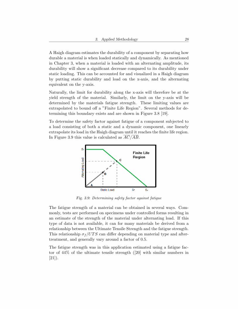
Naturally, the limit for durability along the x-axis will therefore be at theyield strength of the material. Similarly, the limit on the y-axis will bedetermined by the materials fatigue strength. These limiting values areextrapolated to bound o↵ a ”Finite Life Region”. Several methods for de-termining this boundary exists and are shown in Figure 3.8 [19].

To determine the safety factor against fatigue of a component subjected toa load consisting of both a static and a dynamic component, one linearlyextrapolate its load in the Haigh diagram until it reaches the finite life region.In Figure 3.9 this value is calculated as AC/AB.

Fig. 3.9: Determining safety factor against fatigue

The fatigue strength of a material can be obtained in several ways. Com-monly, tests are performed on specimens under controlled forms resulting inan estimate of the strength of the material under alternating load. If thistype of data is not available, it can for many materials be derived from arelationship between the Ultimate Tensile Strength and the fatigue strength.This relationship �

f

/UTS can di↵er depending on material type and after-treatment, and generally vary around a factor of 0.5.

The fatigue strength was in this application estimated using a fatigue fac-tor of 44% of the ultimate tensile strength ([20] with similar numbers in[21]).

4. RESULTS

This chapter describes the results obtained from the methodology describedin Chapter 3.

4.1 Torsional System

The analytical approach of calculating the eigenfrequency of the first tor-sional mode of the condensed system returned a value of 11.7 Hz. Thetorsional system represented by modelling in AVL Excite returned the firsttorsional mode with an eigenfrequency of 11.9 Hz.

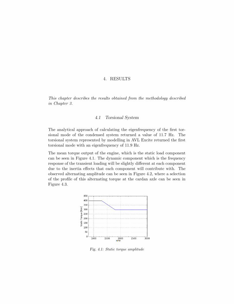
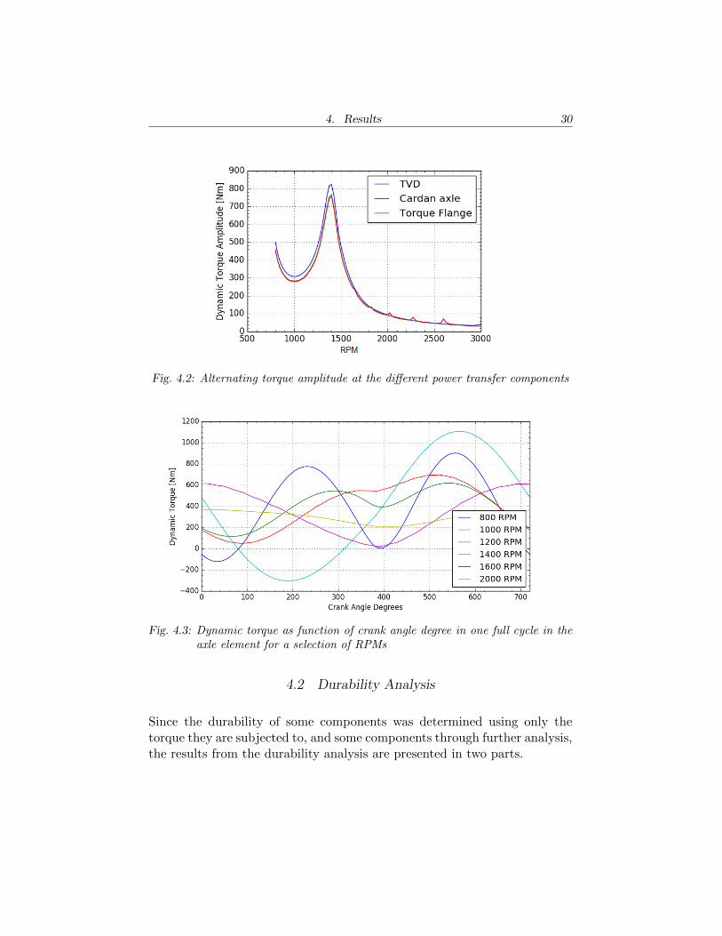
The mean torque output of the engine, which is the static load componentcan be seen in Figure 4.1. The dynamic component which is the frequencyresponse of the transient loading will be slightly di↵erent at each componentdue to the inertia e↵ects that each component will contribute with. Theobserved alternating amplitude can be seen in Figure 4.2, where a selectionof the profile of this alternating torque at the cardan axle can be seen inFigure 4.3.

Fig. 4.1: Static torque amplitude

4. Results 30

Fig. 4.2: Alternating torque amplitude at the di↵erent power transfer components

Fig. 4.3: Dynamic torque as function of crank angle degree in one full cycle in theaxle element for a selection of RPMs

4.2 Durability Analysis

Since the durability of some components was determined using only thetorque they are subjected to, and some components through further analysis,the results from the durability analysis are presented in two parts.

4. Results 31

4.2.1 Load Based Analysis

The torque flange is rated for a nominal torque of 500 Nm [15], a breakingtorque of 400% of the rated torque, a limit torque of 200% of the ratedtorque, and an oscillating peak-to-peak torque of 1000 Nm according toDIN 50100 measurement standards. The torque flange is under worst caseoperation according to the simulation results subjected to a static torque ofjust below 400 Nm and an alternating torque of 750 Nm, meaning that thelimit stated by the manufacturer is exceeded.

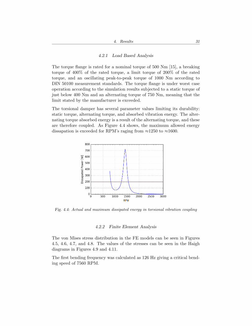
The torsional damper has several parameter values limiting its durability:static torque, alternating torque, and absorbed vibration energy. The alter-nating torque absorbed energy is a result of the alternating torque, and theseare therefore coupled. As Figure 4.4 shows, the maximum allowed energydissapation is exceeded for RPM’s raging from ⇡1250 to ⇡1600.

Fig. 4.4: Actual and maximum dissipated energy in torsional vibration coupling

4.2.2 Finite Element Analysis

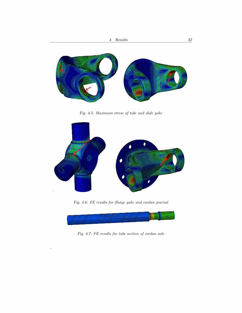
The von Mises stress distribution in the FE models can be seen in Figures4.5, 4.6, 4.7, and 4.8. The values of the stresses can be seen in the Haighdiagrams in Figures 4.9 and 4.11.

The first bending frequency was calculated as 126 Hz giving a critical bend-ing speed of 7560 RPM.

4. Results 32

Fig. 4.5: Maximum stress of tube and slide yoke

Fig. 4.6: FE results for flange yoke and cardan journal

Fig. 4.7: FE results for tube section of cardan axle

.

4. Results 33

Fig. 4.8: FE results for adapter between dyno and torque flange

4.2.3 Fatigue Analysis

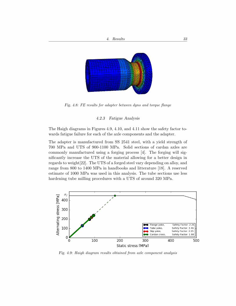
The Haigh diagrams in Figures 4.9, 4.10, and 4.11 show the safety factor to-wards fatigue failure for each of the axle components and the adapter.

The adapter is manufactured from SS 2541 steel, with a yield strength of700 MPa and UTS of 900-1100 MPa. Solid sections of cardan axles arecommonly manufactured using a forging process [4]. The forging will sig-nificantly increase the UTS of the material allowing for a better design inregards to weight[22]. The UTS of a forged steel vary depending on alloy, andrange from 800 to 1400 MPa in handbooks and litterature [18]. A reservedestimate of 1000 MPa was used in this analysis. The tube sections use lesshardening tube milling procedures with a UTS of around 320 MPa.

Fig. 4.9: Haigh diagram results obtained from axle component analysis

4. Results 34

Fig. 4.10: Haigh diagram of axle tube

Fig. 4.11: Haigh diagram of adapter between torque flange and dyno

4.3 Parameter Study

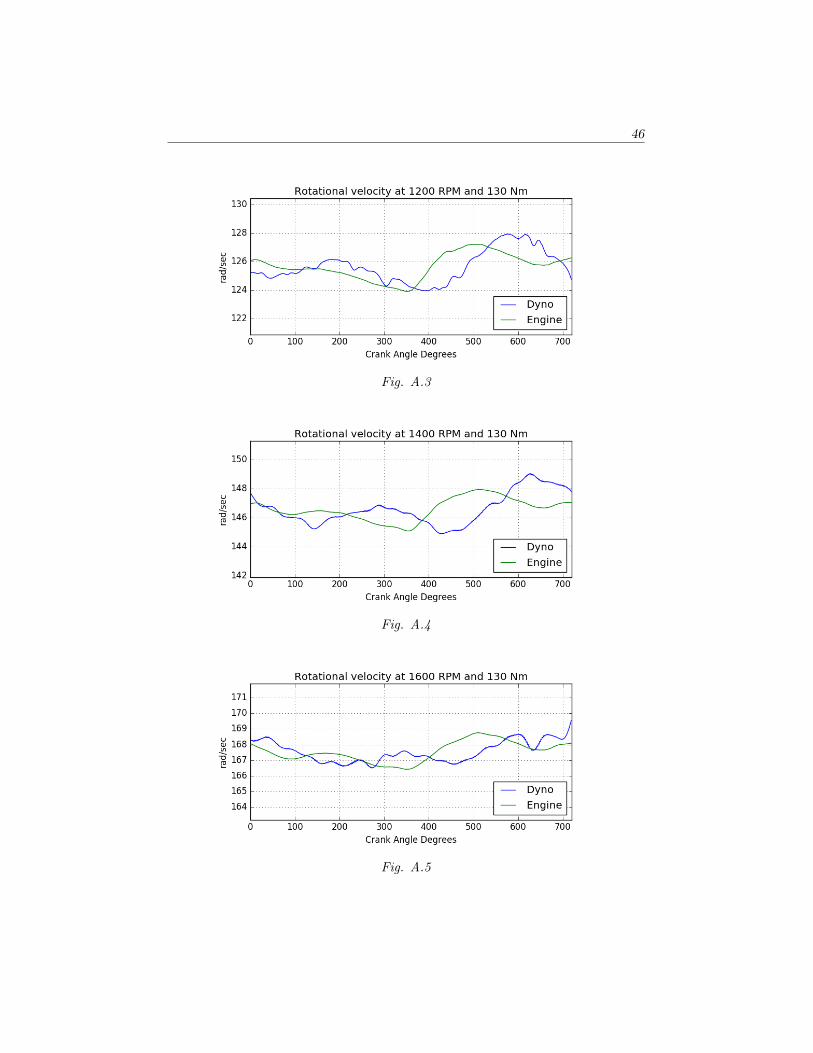
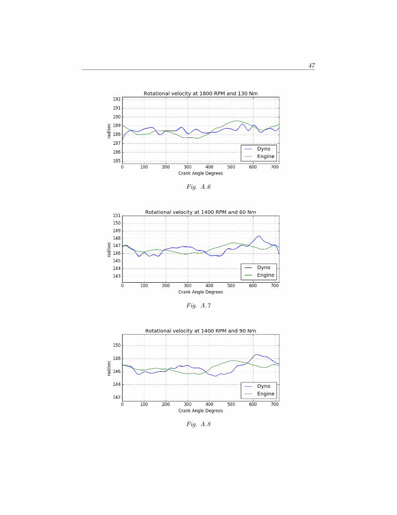
After the rig had been run and tested the results from these tests were com-pared to results obtained from the model. Since these test runs were notconducted at full power, pressure curves obtained for each run during thetesting were used in Excite for the comparison. The full procedure of testingis described in Appendix A.

4. Results 35

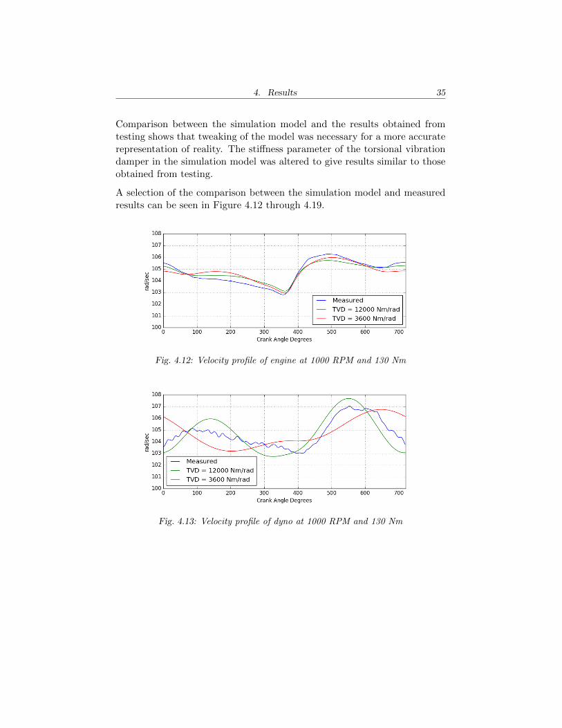
Comparison between the simulation model and the results obtained fromtesting shows that tweaking of the model was necessary for a more accuraterepresentation of reality. The sti↵ness parameter of the torsional vibrationdamper in the simulation model was altered to give results similar to thoseobtained from testing.

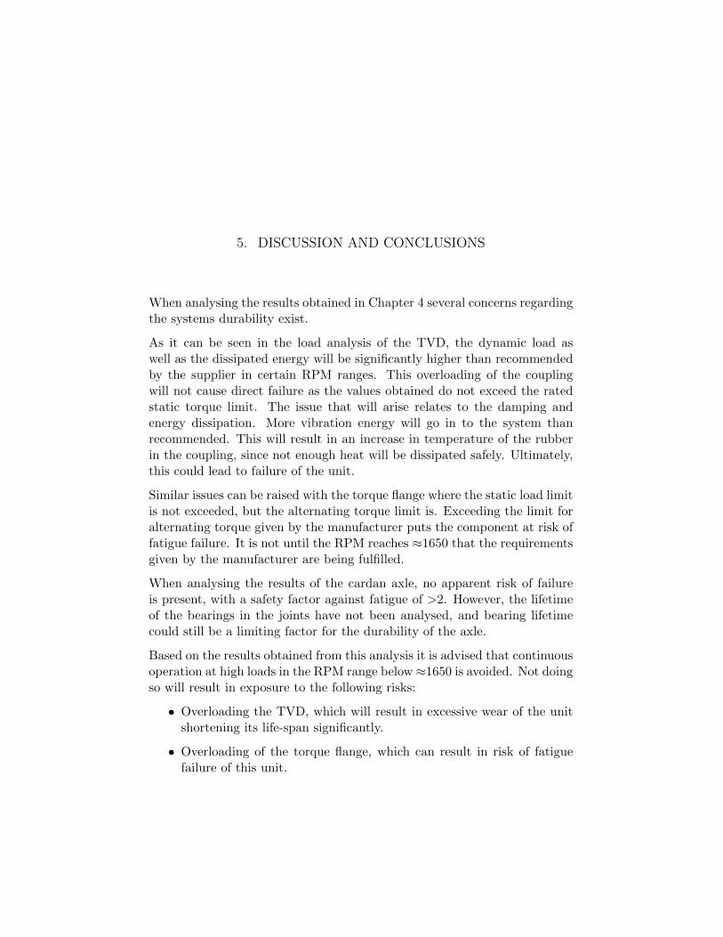
A selection of the comparison between the simulation model and measuredresults can be seen in Figure 4.12 through 4.19.

Fig. 4.12: Velocity profile of engine at 1000 RPM and 130 Nm

Fig. 4.13: Velocity profile of dyno at 1000 RPM and 130 Nm

4. Results 36

Fig. 4.14: Velocity profile of engine at 1400 RPM and 130 Nm



4. Results 37




5. DISCUSSION AND CONCLUSIONS

When analysing the results obtained in Chapter 4 several concerns regardingthe systems durability exist.

As it can be seen in the load analysis of the TVD, the dynamic load aswell as the dissipated energy will be significantly higher than recommendedby the supplier in certain RPM ranges. This overloading of the couplingwill not cause direct failure as the values obtained do not exceed the ratedstatic torque limit. The issue that will arise relates to the damping andenergy dissipation. More vibration energy will go in to the system thanrecommended. This will result in an increase in temperature of the rubberin the coupling, since not enough heat will be dissipated safely. Ultimately,this could lead to failure of the unit.

Similar issues can be raised with the torque flange where the static load limitis not exceeded, but the alternating torque limit is. Exceeding the limit foralternating torque given by the manufacturer puts the component at risk offatigue failure. It is not until the RPM reaches ⇡1650 that the requirementsgiven by the manufacturer are being fulfilled.

When analysing the results of the cardan axle, no apparent risk of failureis present, with a safety factor against fatigue of >2. However, the lifetimeof the bearings in the joints have not been analysed, and bearing lifetimecould still be a limiting factor for the durability of the axle.

Based on the results obtained from this analysis it is advised that continuousoperation at high loads in the RPM range below ⇡1650 is avoided. Not doingso will result in exposure to the following risks:

• Overloading the TVD, which will result in excessive wear of the unitshortening its life-span significantly.

• Overloading of the torque flange, which can result in risk of fatiguefailure of this unit.

5. Discussion and Conclusions 39

A suggestion of action to try to mitigate these issues is to attempt to a↵ectthe eigenfrequencies, for example by altering the system by adding inertiato certain points. An increase of the inertia at the dyno side of the TVDof around 2 kgm2 would move the eigenfrequency causing the peak at 1400significantly, allowing for operation at lower RPM.

What must be considered, when it comes to simulation of dynamic be-haviour, is the issue of determining the validity of the results. The sim-ulation described in this report is based on assumptions of the behaviour ofthe components that might not be accurate, which could a↵ect the outcomeof the analysis.

When looking at the results of the parameter study shown in Figure 4.12through 4.19, it can be seen that for adjusted values of the sti↵ness of theTVD results obtained from the simulation appear to be highly accurate,supporting the validity of the model. When studying these results, it canbe seen that as the load is increased, the sti↵ness yielding accurate resultsdecreases. As sti↵ness is a temperature dependent parameter, this indicatesthat for increased load the temperature of the damper will increase, andeventually reach the value given by the manufacturer of 3600 Nm/rad. Atthis temperature the results from the initial analysis can be expected, andthe conclusions drawn from this analysis deemed reasonable.

6. DELIMITATIONS AND FURTHER STUDIES

The first thing that should be done to verify the results of this simulationis to design an experiment that allows for comparison with experimentalresults. This would be a valuable way to confirm that some of the approxi-mations made are not detrimental to the results.

As discussed in Chapter 2 and 3, one of the assumptions made in the de-scribed method is the use of a completely linear behaviour of the torsionalvibration damper. Preferably, the rubber elasticity and damping constantsare evaluated at more data points to create a more accurate simulationbehaviour of the rubber.

Furthermore, the approach used for evaluation of the fatigue durability is anon-holistic, simplified approach that could be further developed for a moreaccurate description of the failure mode.

Specific calculations on the lifetime expectancy of needle bearings were notconducted due to time restrictions as well as being considered outside thescope of this project. It is recommended to follow the manufacturer recom-mendation regarding bearing lifetime to avoid factors a↵ecting any of theassumptions made in this thesis resulting in other possible causes of failure.The welds used to manufacture the cardan axle were also not accountedfor. However, since the axle was not close to being the weakest component,this is not the recommended first order of action if one were to continue theanalysis.

To develop the model further AVL Excite Power Unit can be used. Thismodule of the Excite interface does not require linear behaviour, whichallows for more complex modelling of joints, TVD parameters, and PIDcontrolled dyno behaviour. This could, especially for more complex systems,result in more accurate modelling, but will require a significantly larger e↵ortfrom the user to get a working model set up properly.

REFERENCES

[1] Figure: Cardan/universal joint [online] http://cdn.pearltrees.com/s/pic/la/cross-joint-72381115 (accessed 01.02.17).

[2] Hans Lundh. Grundlaggande hallfasthetslara. Instutitionen forHallfasthetslara, KTH, 2000.

[3] Huseyin Bayrakceken, Suleyman Tasgetiren, and Ibrahim Yavuz. Twocases of failure in the power transmission system on vehicles: A univer-sal joint yoke and a drive shafts, Engineering Failure Analysis, Volume14(4), p. 716-724, 2007.

[4] David E. Foster, David Crolla, Toshio Kobayashi, and N.D. Vaughan.Encyclopedia of Automotive Engineering. Wiley, International Federa-tion of Automotive Engineering Societies, 2015.

[5] Stephen Timoshenko. Vibration Problems in Engineering. D. Van Nos-trand Company Inc., 2nd edition, 1937.

[6] Troy Feese and Charles Hill. Guidlines for Preventing Torsional Vibra-tion Problems in Reciprocating Machinery. Gas Machinery Conference,Nashville, Tennessee, 7 October 2012.

[7] Bengt Johansson. Combustion Engines. Lunds Tekniska hogskola.

[8] Figure: Four stroke engine [online] https://i2.wp.com/mechstuff.com/wp-content/uploads/2015/10/4-stroke-engine.jpg

(accessed 04.01.17).

[9] AVL Excite Designer User’s Guide. AVL List GmbH, 2016.

[10] Anders K. Olsson. Finite Element Procedures in Modelling the DynamicProperties of Rubber. Doctoral Thesis, Lund University, 2007.

[11] Abaqus Analysis User’s Manual. Dassault Systems Simulia Corp., 2016.

references 42

[12] Anthony Sofranas. Case Histories in Vibration Analysis and MetalFatigue, for the Practicing Engineer. John Wiley and Sons Inc., 2012.

[13] Product Catalog: GKN Stromag highly flexible couplings for universalshafts. GKN Land Systems., 2016.

[14] Product Catalog: Driveline Solutions. GKN Land Systems., 2016.

[15] Data Sheet: T40B Torque Flange. Hottinger Baldwind MesstechnikGmbH, 2016.

[16] Technical Catalog: LSK D.C. motors 2 to 750 kW. Leroy Somer, 2016.

[17] Railway technical handbook, Bearing calculation. SKF Group, 2012.

[18] Bengt Sundstrom (red.). Handbok och formelsamling i hallfasthetslara.Instutitionen for Hallfasthetslara, KTH, 2005.

[19] Figure: Haigh diagram [online] https://becht.com/blog/shaft-

fatigue-failures-part-ii (accessed 15.02.17).

[20] Joseph E. Shigley, Charles R. Mischke, and Thomas H. Brown Jr. Stan-dard Handbook of Machine Design. McGraw-Hill, 3rd edition, 2014.

[21] Stephen R. Schmid, Bernard J. Hamrock, and Bo O. Jacobson. Funda-mentals of Machine Elements. CRC Press, 3rd edition, 2013.

[22] Friedrich Schmelz, Hans C. Seherr-Thoss, and Eirch Aucktor. Universaljoints and driveshafts: analysis, design, applications. Springer-Verlag,1992.

Appendices

43

APPENDIX A

This appendix describes the experimental methodology used to test a torsionalsystems dynamic behaviour and the results of this type of analysis appliedon a test rig at AVL MTC.

Theory and Methodology

This methodology for testing the dynamic behaviour of a torsional sys-tem is an adaptation of a method used for torsional analysis of crankshafts[1].

The analysis relies on measuring the movement of each end of the torsionalsystem using rotational encoders. A rotational encoder is used to convertangular position or motion into a signal that can be registered by a dataacquisition unit. Since one encoder is mounted on the engine for pressuredistribution plots as well as logging of other data and one encoder is mountedat the dyno for control of the RPM, the necessary inputs for the methoddescribed above is available.

The signals from these encoders were fed into a data acquisition unit reg-istering the time taken for each degree of rotation to pass. This value wasinverted to give the rotational velocity and converted into units of radi-ans/second.

Each measurement was run for 30 seconds and the data obtained was aver-aged for each crank angle degree in one full engine cycle (0-720 degrees ofrotation).

The analysis was run at 800 to 1800 RPM in 200 RPM increments with amean torque of 130 Nm, and at 1400 with mean torques ranging between 60and 235 Nm with a total of 6 steps.

[1] Miroslaw Dereszewski, Monitoring of Torsional Vibration of Crankshaftby Instantaneous Angular Speed Observations, Journal of KONES Powertrain and Transport, Volume 23, p. 99-106, 2016

45

Results

The results obtained from the measurement of the velocity profile on theengine as well as the dyno can be seen in Figures A.1 through A.11.

Fig. A.1

Fig. A.2

46

Fig. A.3

Fig. A.4

Fig. A.5

47

Fig. A.6

Fig. A.7

Fig. A.8

48

Fig. A.9

Fig. A.10

Fig. A.11

www.kth.se

Date post:	28-Mar-2018
Category:	Documents
Upload:	vophuc
View:	221 times
Download:	2 times

Dynamic Simulation of a One Cylinder Engine Test...

Documents