ORIGINAL PAPER

Dynamic Sliding Analysis of a Gravity Dam with Fluid-Structure-Foundation Interaction Using Finite Elements and Newmark’sSliding Block Analysis

Markus Goldgruber • Shervin Shahriari •

Gerald Zenz

Received: 7 July 2014 / Accepted: 18 January 2015 / Published online: 28 January 2015

� Springer-Verlag Wien 2015

Abstract To reduce the natural hazard risks—due to,

e.g., earthquake excitation—seismic safety assessments are

carried out. Especially under severe loading, due to maxi-

mum credible or the so-called safety evaluation earth-

quake, critical infrastructure, as these are high dams, must

not fail. However, under high loading local failure might be

allowed as long as the entire structure does not collapse.

Hence, for a dam, the loss of sliding stability during a short

time period might be acceptable if the cumulative dis-

placements after an event are below an acceptable value.

This performance is not only valid for gravity dams but

also for rock blocks as sliding is even more imminent in

zones with higher seismic activity. Sliding modes cannot

only occur in the dam-foundation contact, but also in

sliding planes formed due to geological conditions. This

work compares the qualitative possible and critical dis-

placements for two methods, the well-known Newmark’s

sliding block analysis and a Fluid-Foundation-Structure

Interaction simulation with the finite elements method. The

results comparison of the maximum displacements at the

end of the seismic event of the two methods depicts that for

high friction angles, they are fairly close. For low friction

angles, the results are differing more. The conclusion is

that the commonly used Newmark’s sliding block analysis

and the finite elements simulation are only comparable for

high friction angles, where this factor dominates the

behaviour of the structure. Worth to mention is that the

proposed simulation methods are also applicable to

dynamic rock wedge problems and not only to dams.

Keywords Sliding analysis � Gravity dam � Earthquake �Newmark � Fluid-structure-foundation interaction

List of Symbols

€arel Relative acceleration

t Time

a Acceleration

ay Yield acceleration

ls Friction coefficient

Hs Hydrostatic force

W Deadweight of the structure

G Gravity

Hd Hydrodynamic force

Phd Hydrodynamic pressure

z Water height variable from bottom to top of the

structure

mw Added mass according to the simplified

Westergaard formula

h Total water depth

qw Water density

f Friction force before the structure starts to slide

M Mass of the structure

U Uplift force in the structure-foundation plane

av Vertical acceleration

DN Newmark displacement according to empirical

formulas in centimeters

amax Maximum acceleration out of time history

IA Arias intensity

Td Duration of the ground motion

m�w Added mass according to the rigorous Westergaard

formula

M. Goldgruber (&) � S. Shahriari � G. Zenz

Institute of Hydraulic Engineering and Water Resources

Management, TU Graz, Stremayrgasse 10/II, 8010 Graz, Austria

e-mail: markus.goldgruber@tugraz.at

S. Shahriari

e-mail: shervin.shahriari@student.tugraz.at

G. Zenz

e-mail: gerald.zenz@tugraz.at

123

Rock Mech Rock Eng (2015) 48:2405–2419

DOI 10.1007/s00603-015-0714-1

n Mode number used for the added mass calculation

cn Constant factor for the added mass calculation

K Compressibility (Bulk modulus) of the water

T Eigenperiod of the reservoir

f Eigenfrequency of the reservoir

cw Wave propagation speed in the water

v Velocity vector

r Nabla operator

P Acoustic pressure

a Mass-proportional damping

b Stiffness-proportional damping

f Critical damping factor

xi First eigenfrequency for the Rayleigh damping

calculation

xj Second eigenfrequency for the Rayleigh damping

calculation

1 Introduction

Investigations of the sliding stability of gravity dams and

rock blocks at seismic loading depicts that many additional

factors are influencing the dynamic behaviour of the sys-

tem. Treating the gravity dam as rigid block may lead to

wrong results regarding stresses and displacements, due to

the self-oscillations of the structure. Additionally to the

dynamic load from the excited structure and water, there

are also static loads acting on the structure like the

hydrostatic water load and the pore water pressure in the

contact plane, which is also influenced by a grout curtain,

drainage systems and fault zones. Due to the self-weight,

we get the shear force and cohesion in the contact plane

according to the Mohr–Coulomb failure criterion, which

are the only two parameters against sliding of the model.

Gravity dam stability against sliding failure mechanism

(under seismic conditions/loading) can be assessed by

following different approaches:

• Limit equilibrium method considering the inertial

forces as static permanent loads.

• Newmark’s sliding block analysis or dynamic simpli-

fied approach, which computes the permanent displace-

ment of a rigid block under seismic excitation.

• True dynamic analyses with the finite elements method

(FEM).

The simplified and the true dynamic analyses lead to the

evaluation of the relative displacement of the gravity dam.

The relative displacement is the fundamental requirement

to assess the dam safety.

Newmark (1965) derived an analytical method to cal-

culate the possible displacements of embankments dams

based on a critical acceleration at which sliding starts. In the

past and now, this method is also used for rock sliding

evaluation for seismic loadings. Later, based on Newmark’s

Sliding Block Analysis, Chopra and Hall (1982) derived the

critical acceleration for gravity dam structures or more

generally speaking, structures which are also loaded by

water pressures and uplift and not just by deadweight.

Besides the analytical ways, contact modelling with

finite elements is a complicated numerical procedure. It

gets even harder if the problem is dynamic. Many param-

eters, e.g., time integration schemes and time integration

factors may be influencing the results significantly.

Therefore, dynamic investigations of structures with con-

tact modelling must be examined critically.

For the Fluid–structure interaction (FSI) simulation in

the finite elements method, one has several possibilities to

do that. The added mass technique is still commonly used

by consultants, because of its easy way to implement and

its conservative results, compared to more sophisticated

ways to model the water. Another popular way to model

the interaction problem with resting water, e.g., a reservoir,

is to do it with acoustic elements, with pressure as their

only variable. Other possibilities of discretisation are the

eulerian or lagrangian approach, fluid elements (CFD) or

the smoothed particle hydrodynamics method (SPH).

This work should give a comparison between the

Newmark based sliding block method published by Chopra

and Hall (1982), different empirical formulas like those

from Jibson (1993), Jibson, Harp and Michael (1998) and

Ambrasey and Menu (1988), and the finite elements

method utilizing added masses and acoustic elements. It

should also show the applicability of these different

methods to sliding problems of gravity dams and rock

blocks interacting with the water.

1.1 Gravity Dam Model

The structure of interest is a concrete gravity dam. The

focus of this work is the sliding safety of such a structure

on a horizontal rock foundation due to seismic loading.

The geometry of the gravity dam is based on the

dimensions of the Birecik dam (Fig. 1) and has, therefore, a

height of 62.5 m. The base of the dam has a width of

45.0 m. A grout curtain is situated 7 m in distance from the

upstream surface of the dam and it reaches 30 m into the

foundation. This leads to an uplift pressure decrease to 2/3

of the maximum pressure (Fig. 2) from the reservoir water

level, which is a common assumption for safety assess-

ments of concrete dams for simplified methods.

In the case of a seismic event, it cannot be ensured that

the grout curtain is still working properly. So, the conser-

vative assumption was made that the pore water pressure

distribution will be linear from the upstream to the

2406 M. Goldgruber et al.

123

downstream side. Such a distribution can be assumed as a

post-earthquake case.

Additional investigations of the whole model have been

done with a scale factor of 2.0. This means that the height

of the dam is increased to 125 m. This is done to evaluate

the influence of scaling effects of the modelling techniques

explained in Sect. 2.2.3.

1.2 Earthquake Acceleration Records

Acceleration time histories are based on design spectra

according to the peak ground acceleration (PGA) and the

normalized spectra for a specific area. To define such a

spectrum, mostly empirical methods are used. Some of

them are:

• The Newmark method for spectra,

• the US-NRC spectra from the United States,

• the HSK-spectra from Switzerland and

• a study on spectra by McGuire (1974).

The one used in the Austrian guideline for earthquake

assessment of dams by the Bundesministerium fur Land-

und Forstwirtschaft (2001) is based on the study by

McGuire (1974), which is only applicable to rock foun-

dations and alluvium. These spectra are not applicable to

underground conditions where significant amplifications

due to sediments are expected. In this case, further studies

on the influence of the underground have to be done.

For nonlinear assessments of structures time-histories of

the ground acceleration are needed. The two orthogonal

independent acceleration time histories used in this study are

shown in Fig. 3 and generated according to the spectra from

the Austrian guideline mentioned above, by using the program

SIMQKE from Massachusetts Institute of Technology (1976).

From a practical point of view, using just one artificial

acceleration record has the drawback that it only covers one

specific frequency range; therefore, the use of several different

records for the practical assessment of seismic excited struc-

tures is recommended, because the exact amplitude or fre-

quency of an earthquake is not predictable. A simplification

often done by engineers is to scale the records to increase or

decrease the amplitude, without changes in the frequency

range. However, measurements of real earthquakes have

shown that the frequency changes with the intensity. There-

fore, the applied motion can lead to conservative or under

estimated results. This means that the consideration of the

expected amplitude in coherence with the frequency is

unconditionally recommended for the assessment.

The accelerations in the model are applied in both

directions, horizontal (x) and vertical (y), on the foundation

boundaries in normal direction with a maximum acceler-

ation of 1.0 m/s2.

2 Methods

2.1 Newmark’s Sliding Block Analysis

The pseudo-static method of analysis provides the factor of

safety but no information on deformations associated with

Fig. 1 Gravity dam model and dimensions

Fig. 2 Uplift distribution with (left) and without grout curtain (right)

Fig. 3 Acceleration time history records

Dynamic Sliding Analysis of a Gravity 2407

123

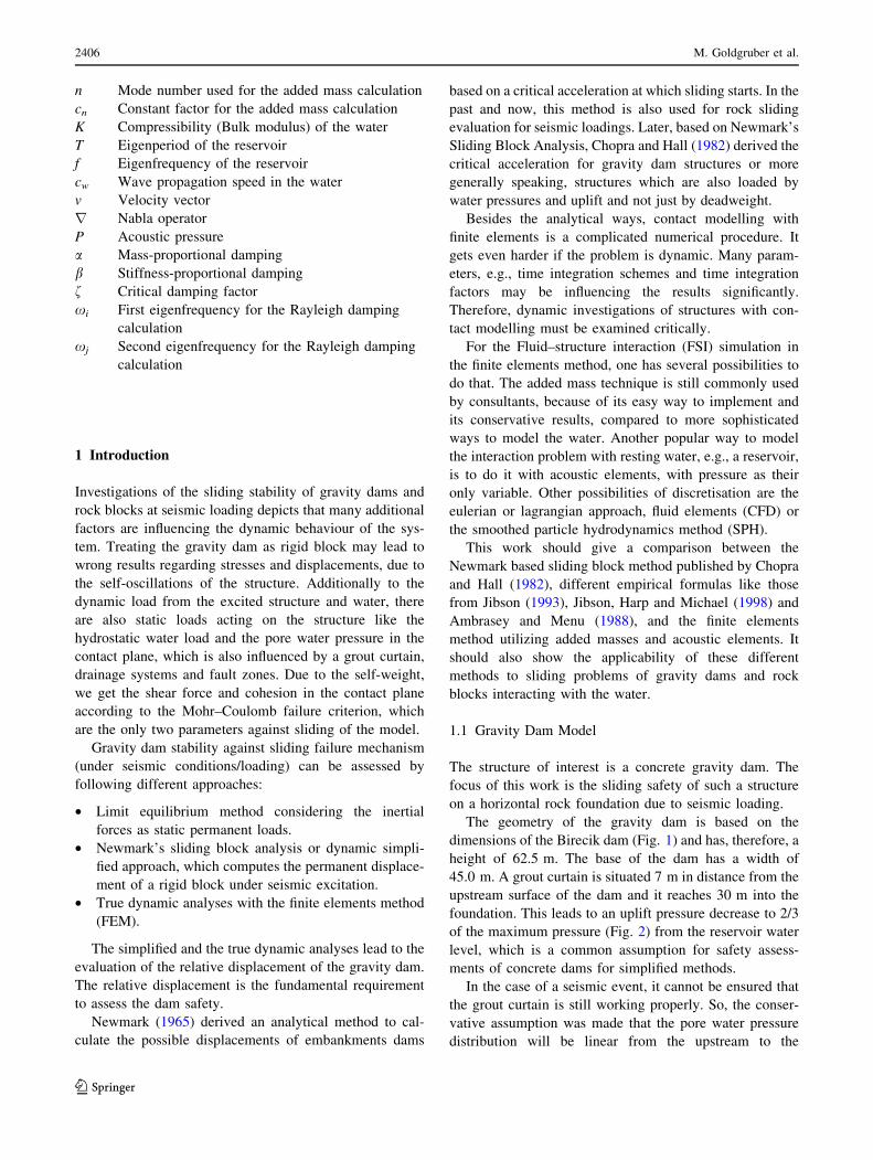
the failure. Since earthquake-induced accelerations vary

with time, the pseudo-static factor of safety will vary

throughout a ground motion. Newmark (1965) proposed a

method of analysis that estimates the permanent displace-

ment of a slope subjected to ground motions by assuming a

rigid block resting on an inclined plane. When a block is

subjected to a pulse of acceleration that exceeds the yield

acceleration, the block will move relative to the ground.

The relative acceleration is given by:

€arel tð Þ ¼ a tð Þ � ay

where €arel is the relative acceleration of the block, a(t) is

the ground acceleration at time t and ay is the yield

acceleration. By integrating the relative acceleration twice

and assuming linear variation of acceleration the relative

velocity and displacement at each time increment can be

obtained (Fig. 4).

Sliding is initiated in the downstream direction when the

upstream ground acceleration a(t) exceeds the yield

acceleration ay. Downstream sliding ends when the sliding

velocity €arel is zero and the ground acceleration drops

below the yield acceleration.

2.1.1 Yield Accelerations

Conducting a Newmark analysis requires characterization

of two key elements. The first element is the dynamic

stability of the rigid block and it can be quantified as the

yield or critical acceleration ay. This parameter is the

threshold ground acceleration necessary to overcome slid-

ing resistance force and initiate permanent block move-

ment. The second parameter is the ground motion record to

which the block will be subjected.

To perform a Newmark analysis, the gravity dam

assumed to be a rigid body of mass M and weight W sup-

ported on horizontal ground that is subjected to accelera-

tion a(t). In reality, the dam is bonded to the foundation;

however, in this study the dam is assumed to rest on hor-

izontal ground without any mutual bond and the only force

against sliding of the dam is the friction force between the

base of the dam and the ground surface. Selecting an

appropriate friction coefficient ls is complicated because

after earthquake forces overcome the bond between dam

and foundation rock, the cracked surface will be rough and

the friction coefficient for such a surface is significantly

higher than for a planar dam-foundation interface.

The hydrostatic force Hs acting on the face of the dam is

always pushing the dam in the downstream direction.

The inertia force associated with the mass of the dam is

-(W/g)a(t) and it is acting opposite to the acceleration

direction. The hydrodynamic force can be determined as

below:

Hd tð Þ ¼ �a tð ÞZ

Phd zð Þdz ¼ �mwðzÞa tð Þ;

where Phd(z) is the hydrodynamic pressure on the upstream

face of the dam due to unit acceleration in the upstream

direction and mw(z) is the added mass which moves with the

dam and produces inertia force. The added massmw(z) can be

determined by Westergaard’s (1933) equation as below:

mwðzÞ ¼Zh

0

7

8qw

ffiffiffiffiffihz

pdz ¼ 0:583qh2;

where qw is the density of water.

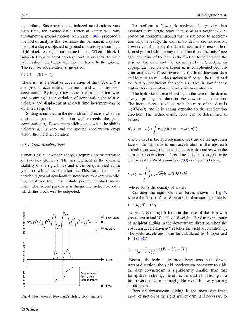
Consider the equilibrium of forces shown in Fig. 5,

where the friction force F before the dam starts to slide is:

F ¼ ls W � Uð Þ;

where U is the uplift force at the base of the dam with

grout curtain and W is the deadweight. The dam is in a state

of incipient sliding in the downstream direction when the

upstream acceleration a(t) reaches the yield acceleration ay.

The yield acceleration can be calculated by Chopra and

Hall (1982):

ay ¼1

M þ mwðzÞls W � Uð Þ � Hs½ �

Because the hydrostatic force always acts in the down-

stream direction, the yield acceleration necessary to slide

the dam downstream is significantly smaller than that

for upstream sliding; therefore, the upstream sliding in a

full reservoir case is negligible even for very strong

earthquakes.

Because downstream sliding is the most significant

mode of motion of the rigid gravity dam, it is necessary toFig. 4 Illustration of Newmark’s sliding block analysis

2408 M. Goldgruber et al.

123

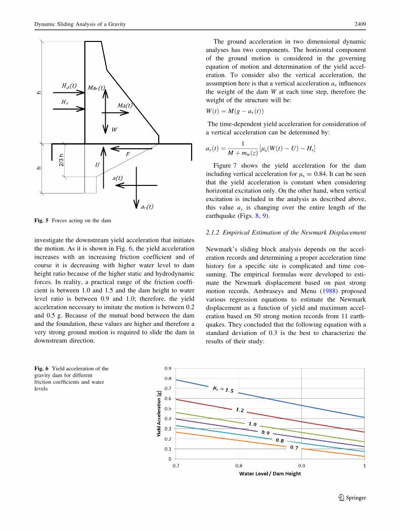
investigate the downstream yield acceleration that initiates

the motion. As it is shown in Fig. 6, the yield acceleration

increases with an increasing friction coefficient and of

course it is decreasing with higher water level to dam

height ratio because of the higher static and hydrodynamic

forces. In reality, a practical range of the friction coeffi-

cient is between 1.0 and 1.5 and the dam height to water

level ratio is between 0.9 and 1.0; therefore, the yield

acceleration necessary to imitate the motion is between 0.2

and 0.5 g. Because of the mutual bond between the dam

and the foundation, these values are higher and therefore a

very strong ground motion is required to slide the dam in

downstream direction.

The ground acceleration in two dimensional dynamic

analyses has two components. The horizontal component

of the ground motion is considered in the governing

equation of motion and determination of the yield accel-

eration. To consider also the vertical acceleration, the

assumption here is that a vertical acceleration av influences

the weight of the dam W at each time step, therefore the

weight of the structure will be:

W tð Þ ¼ M g� av tð Þð Þ

The time-dependent yield acceleration for consideration of

a vertical acceleration can be determined by:

ayðtÞ ¼1

M þ mwðzÞls W tð Þ � Uð Þ � Hs½ �

Figure 7 shows the yield acceleration for the dam

including vertical acceleration for ls = 0.84. It can be seen

that the yield acceleration is constant when considering

horizontal excitation only. On the other hand, when vertical

excitation is included in the analysis as described above,

this value ay is changing over the entire length of the

earthquake (Figs. 8, 9).

2.1.2 Empirical Estimation of the Newmark Displacement

Newmark’s sliding block analysis depends on the accel-

eration records and determining a proper acceleration time

history for a specific site is complicated and time con-

suming. The empirical formulas were developed to esti-

mate the Newmark displacement based on past strong

motion records. Ambraseys and Menu (1988) proposed

various regression equations to estimate the Newmark

displacement as a function of yield and maximum accel-

eration based on 50 strong motion records from 11 earth-

quakes. They concluded that the following equation with a

standard deviation of 0.3 is the best to characterize the

results of their study:

Fig. 5 Forces acting on the dam

Fig. 6 Yield acceleration of the

gravity dam for different

friction coefficients and water

levels

Dynamic Sliding Analysis of a Gravity 2409

123

logDN ¼ 0:90 þ log 1 � ay

amax

� �2:53ay

amax

� ��1:09 !

� 0:30;

where ay is the yield acceleration, amax is the maximum

acceleration and DN is the Newmark displacement in

centimeters. Different forms of equations have been pro-

posed in other studies with additional parameters to esti-

mate Newmark’s displacement. Jibson (1993), proposed

the following regression equation which is known as Jib-

son93 and it is based on 11 acceleration records which are

suitable for ay values of 0.02, 0.05, 0.10, 0.20, 0.30 and

0.40 g with a standard deviation of 0.409:

logDN ¼ 1:460 log IA � 6:641ay þ 1:546 � 0:409;

where ay is the yield acceleration in g’s, IA is the Arias

intensity in meters per second and DN is the Newmark

displacement in centimeters. The Arias intensity (Arias

1970) is a measure of the strength of a ground motion and

can be determined by the equation

IA ¼ p2g

ZTd

0

a2ðtÞdt;

where g is the gravity, a(t) is the ground motion accelera-

tion and Td is the duration of the ground motion. The Arias

intensity measures the total acceleration content of the

records and it provides a better parameter for describing the

content of the strong motion record than does the peak

acceleration. In the Jibson93 equation, ay is a linear term

and it makes the model overly sensitive to small changes of

yield acceleration. Jibson et al. (1998) modified the equa-

tion to make all terms logarithmic and then performed a

rigorous analysis of 555 strong motion records from 13

earthquakes for the same ay values as indicated for Jib-

son93 to generate the following regression equation:

logDN ¼ 1:521 log IA � 1:993ay � 1:546 � 0:375

2.2 The Numerical Method

2.2.1 2D Structural Finite Element Model

The 2D structural model contains three parts, the gravity

dam, the foundation and the reservoir, which are assembled

together by specific interaction conditions. The finite ele-

ments dam model is discretized with linear quadrilateral

and triangular elements. The linear triangular elements are

only used near the contact surface between dam and

foundation, because of the mesh refinement, due to the use

of linear elements. The finite element foundation model has

a total length of 300.0 m and a height of 100.0 m. The

boundaries are fixed normal to their surface for static

loading conditions. This model is fully discretized with

linear quadrilateral elements.

Furthermore, to evaluate the effects of the interaction

with the added mass method compared to the model with

the acoustic volume according to Sect. 2.2.3, a second

model has been made and scaled by the factor of 2.0,

resulting in a height of 125.0 m.

2.2.2 Contact Modelling

Besides the structural modelling, the contacts between the

different parts have to be defined. For the interaction of the

gravity dam and the reservoir, the coupling is set to ‘‘tie

constraint’’, so no relative movement is possible.

The interaction modelling between the dam and the

foundation is more complicated. The contact modelling

parameters have been chosen as simple as possible to get

proper and converging results, which could not be that easy

to achieve in a transient dynamic simulation. The contact in

ABAQUS/CAE is defined as finite sliding with a ‘‘surface

to surface’’ discretization. For the tangential behaviour, the

penalty formulation is used, which means that the friction

angle and a maximum elastic slip have to be specified. The

friction angle is changed in each simulation separately and

Fig. 7 Yield acceleration

including vertical acceleration

for a case with ls = 0.884

2410 M. Goldgruber et al.

123

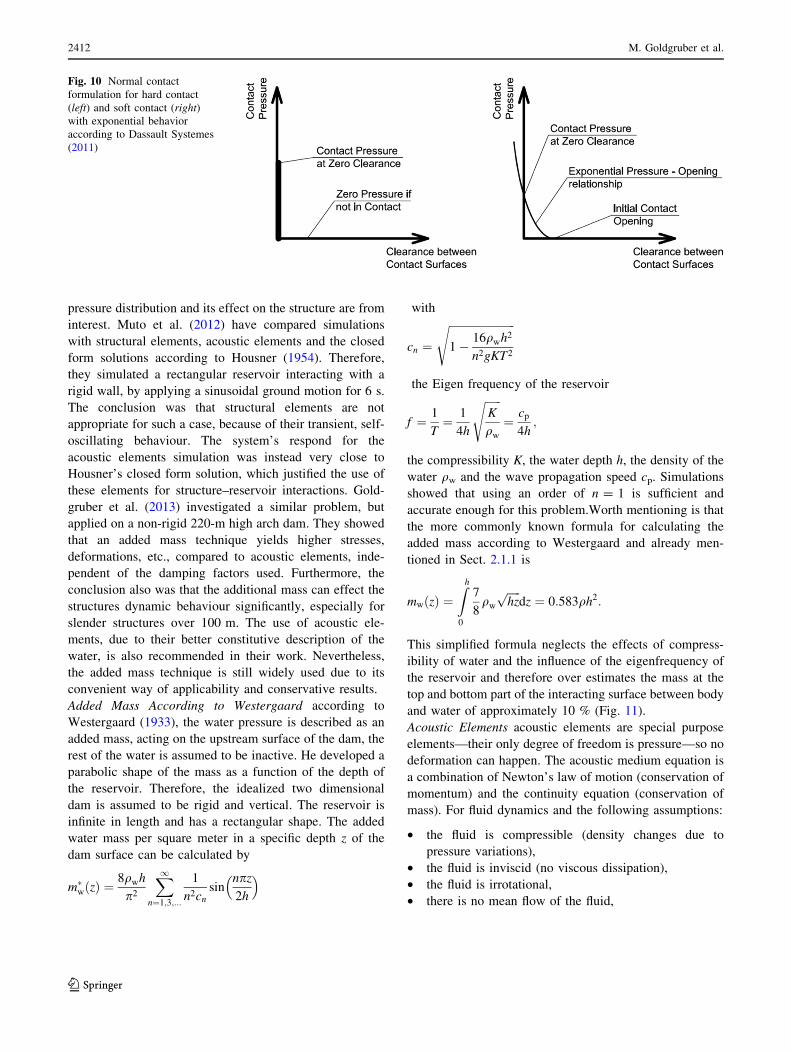
for the elastic slip, the default value for the slip tolerance of

0.005 (0.5 %) is used. This value is defined as the ratio of

allowable maximum elastic slip to characteristic contact

surface face dimension. An exceedance of this value results

in permanent displacement. One can increase this value for

better computational efficiency, but therefore losing

accuracy.

The cohesion is neglected in these simulations, so the

friction angles used, can be understood as the residual

friction angle.

The normal contact formulation is set to ‘‘Hard Contact’’

(Fig. 10). Additionally to these parameters, any separation

of the contact surfaces is neglected, to reach convergence

more easily. Another possibility would be the use of the

‘‘Soft Contact’’ formulation with, e.g., ‘‘Exponential Pres-

sure–Opening relationship’’ shown in Fig. 10, but hasn’t

been used for these simulations. The contact modelling and

the accompanying convergence problems are also the main

reason for using linear elements instead of quadratic ones.

The simulations of the models with a height of 62.5 and

125.0 m, respectively, and also for the two reservoir

modelling techniques described in Sect. 2.2.3 are per-

formed for different friction angles and zero inclination in

the contact plane. The friction coefficient starts at 1.0 (45�)and is reduced in 5 steps until the displacement is getting

progressive. Table 2 shows the friction coefficients and

corresponding friction angles used for the simulations.

2.2.3 Reservoir Modelling

The first and the easiest way to model the water is to treat it

as an additional attached mass onto the upstream surface of

the dam. The water mass is increasing with the depth of the

reservoir. Two different ways to calculate the added water

mass are used. For the application of these masses in the

ABAQUS/CAE model of the dam, a user subroutine called

UEL (User Element) was written. This subroutine calcu-

lates the mass for every node of an element surface, e.g.,

three nodes for a quadratic formulation and two nodes for a

linear shell element, and distributes it evenly. To define the

element surface on which the mass is acting, a Python

script was written, which extracts the nodes of the specific

surfaces automatically and writes it back to input file of the

model. The added mass technique used in this work is the

one proposed by Westergaard (1933), which is the most

common. Usually, engineers are using the simplified for-

mula, which neglects the compressibility. This work will

show some major differences between the application of

the simplified and rigorous formula.

Additionally to the added mass techniques by West-

ergaard (1933), the Fluid-Structure Interaction is also

modelled with so-called Acoustic Elements. These ele-

ments are commonly used in pressure and sound wave

simulations, but give some major advantages for problems

where a volume of water is excited moderately (e.g., water

reservoirs, cooling tanks, etc.). For such problems the

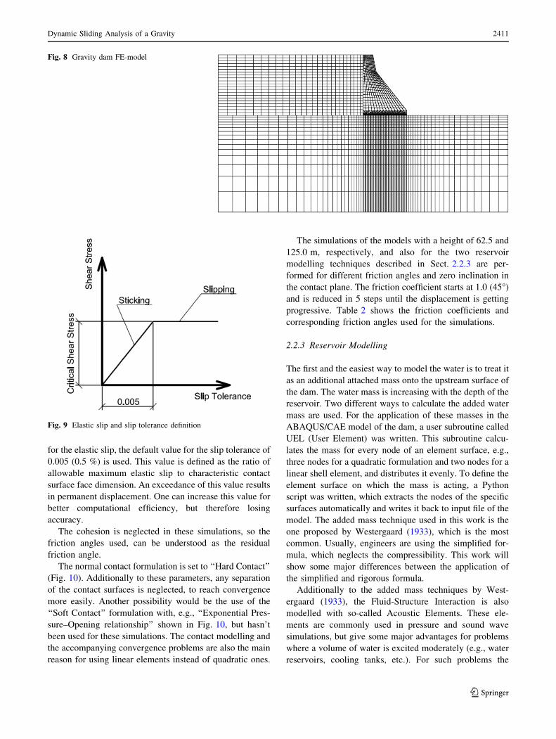
Fig. 8 Gravity dam FE-model

Fig. 9 Elastic slip and slip tolerance definition

Dynamic Sliding Analysis of a Gravity 2411

123

pressure distribution and its effect on the structure are from

interest. Muto et al. (2012) have compared simulations

with structural elements, acoustic elements and the closed

form solutions according to Housner (1954). Therefore,

they simulated a rectangular reservoir interacting with a

rigid wall, by applying a sinusoidal ground motion for 6 s.

The conclusion was that structural elements are not

appropriate for such a case, because of their transient, self-

oscillating behaviour. The system’s respond for the

acoustic elements simulation was instead very close to

Housner’s closed form solution, which justified the use of

these elements for structure–reservoir interactions. Gold-

gruber et al. (2013) investigated a similar problem, but

applied on a non-rigid 220-m high arch dam. They showed

that an added mass technique yields higher stresses,

deformations, etc., compared to acoustic elements, inde-

pendent of the damping factors used. Furthermore, the

conclusion also was that the additional mass can effect the

structures dynamic behaviour significantly, especially for

slender structures over 100 m. The use of acoustic ele-

ments, due to their better constitutive description of the

water, is also recommended in their work. Nevertheless,

the added mass technique is still widely used due to its

convenient way of applicability and conservative results.

Added Mass According to Westergaard according to

Westergaard (1933), the water pressure is described as an

added mass, acting on the upstream surface of the dam, the

rest of the water is assumed to be inactive. He developed a

parabolic shape of the mass as a function of the depth of

the reservoir. Therefore, the idealized two dimensional

dam is assumed to be rigid and vertical. The reservoir is

infinite in length and has a rectangular shape. The added

water mass per square meter in a specific depth z of the

dam surface can be calculated by

m�wðzÞ ¼

8qwh

p2

X1n¼1;3;...

1

n2cnsin

npz2h

� �

with

cn ¼

ffiffiffiffiffiffiffiffiffiffiffiffiffiffiffiffiffiffiffiffiffiffiffiffi1 � 16qwh

2

n2gKT2

s

the Eigen frequency of the reservoir

f ¼ 1

T¼ 1

4h

ffiffiffiffiffiffiK

qw

s¼ cp

4h;

the compressibility K, the water depth h, the density of the

water qw and the wave propagation speed cp. Simulations

showed that using an order of n = 1 is sufficient and

accurate enough for this problem.Worth mentioning is that

the more commonly known formula for calculating the

added mass according to Westergaard and already men-

tioned in Sect. 2.1.1 is

mwðzÞ ¼Zh

0

7

8qw

ffiffiffiffiffihz

pdz ¼ 0:583qh2:

This simplified formula neglects the effects of compress-

ibility of water and the influence of the eigenfrequency of

the reservoir and therefore over estimates the mass at the

top and bottom part of the interacting surface between body

and water of approximately 10 % (Fig. 11).

Acoustic Elements acoustic elements are special purpose

elements—their only degree of freedom is pressure—so no

deformation can happen. The acoustic medium equation is

a combination of Newton’s law of motion (conservation of

momentum) and the continuity equation (conservation of

mass). For fluid dynamics and the following assumptions:

• the fluid is compressible (density changes due to

pressure variations),

• the fluid is inviscid (no viscous dissipation),

• the fluid is irrotational,

• there is no mean flow of the fluid,

Fig. 10 Normal contact

formulation for hard contact

(left) and soft contact (right)

with exponential behavior

according to Dassault Systemes

(2011)

2412 M. Goldgruber et al.

123

• the mean density and pressure are uniform throughout

the fluid,

• no body forces and

• a homogeneous medium

the equation of motion for an acoustic medium can be

written as

q0

ov

otþrpðtÞ ¼ 0

and the continuity equation gives

oqðtÞot

þ q0r � v ¼ 0

The constitutive law and hence the relationship between

the pressure and density for an acoustic medium is defined

as

op tð Þ ¼ c2woq tð Þ;

with cw as the wave propagation speed in the water, which

is assumed to be constant.Combining these three equations

finally results in the linear acoustic wave equation, with the

only degree of freedom p(t)

o2pðtÞot2

� c2wr2p tð Þ ¼ 0:

The acoustic volume has a length of 150.0 m (300.0 m for the

two times scaled model) and the same height as the gravity

dam model. The same elements are used as for the foundation.

The boundary condition on the upstream end of the reservoir is

set to non-reflecting, which means that the pressure is com-

pletely absorbed, this boundary formulation is described by

Lysmer and Kuhlemeyer (1969). Furthermore, on the water

surface, the acoustic pressure is set to zero.

2.2.4 Grout Curtain and Pore Water Pressure

The grout curtain is situated 7 m away from the upstream

surface of the dam and reaches 30 m into the rock

foundation. The distribution of the pore water pressure in

the foundation is simulated in a steady-state step for full

reservoir conditions (62.5 and 125.0 m) on the upstream

side and zero on the downstream side. The permeability of

the rock and the grout is written down in Table 1. In an

earthquake scenario, one cannot necessarily assume that

the grout curtain will still be fulfilling its purpose. For this

case the pore water pressure distribution under the structure

is assumed linear. This effect on the systems behaviour is

also examined.

2.2.5 Structural Damping

For all simulations Rayleigh Damping is applied to the

model. According to the fact that tests on existing dam

structures showed that the critical damping factor can vary

between 3 and 10 % according to Selecting Seismic

Parameters for Large Dams Guidelines (2010), the critical

damping factor used is 5 %. For the damping of the rock

mass, the simplification has been made, that the same

Rayleigh damping factors are used as for the dam structure.

The mass-proportional factor for two specific Eigen

frequencies and the critical damping is calculated with

a ¼ f2xixj

xi þ xj

and the stiffness-proportional damping with

b ¼ f2

xi þ xj

For the two different heights, 62.5 and 125.0 m, and two

different modelling techniques of the water, one gets 4

models to calculate the Rayleigh damping factors. The

frequencies and corresponding modes of the structure cal-

culated with a numerical software must be examined in

detail. Some modes, especially when acoustic elements are

used, are not contributing to the structures behavior. This

modes and frequencies have been filtered based on the

Fig. 11 Westergaard added

mass behaviour between the

simplified and the rigorous

formula

Dynamic Sliding Analysis of a Gravity 2413

123

participating factors and mass contribution. This means,

modes with a low effective mass contribution have been

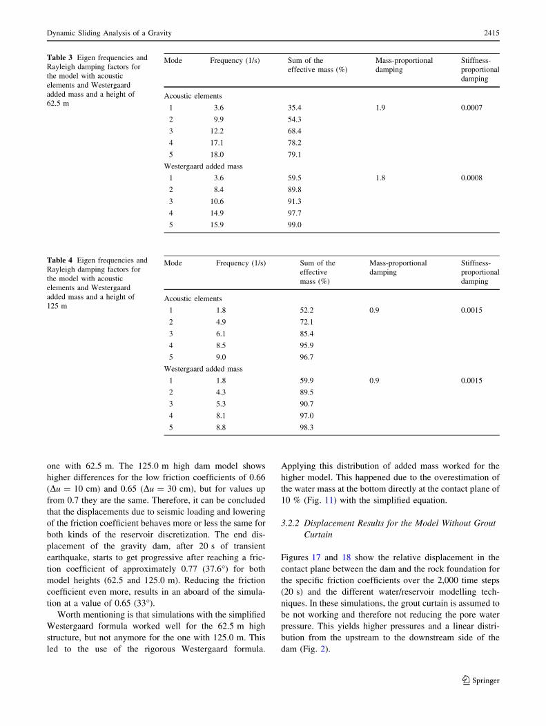
neglected. In Tables 3 and 4, the frequencies and the cor-

responding Rayleigh damping factors for the four models

are listed. The mass and stiffness-proportional damping

factors have been calculated for the 1st and 5th eigenfre-

quency for each of the four models, based on the sum of the

effective mass. All models but the one with acoustic ele-

ments and a height of 62.5 m are reaching a percentage of

more than 90 %. The two used frequencies for the damping

factors are left the same to make it more comparable to the

one with the Westergaard added mass (Table 4).

2.2.6 Dynamic Modelling

In the final step of the simulation, the seismic loading is applied.

The accelerations are acting in horizontal (x) and vertical

(y) direction on the foundation boundaries. For solving the

equation of motion, implicit direct time integration according to

Hilber et al. (1977) is used. Because of convergence issues in

the contact modelling, the time integration parameter a is set to

-0.333. This value accounts for maximum numerical damp-

ing, which means that the high frequency responses of the

structure are neglected and convergence is reached more easily.

The accelerations in the time histories are defined for every

0.01 s. Therefore, for each simulation one has 2,000 time steps

for the 20 s seismic event. The acceleration time histories are

depicted in Fig. 3 in Sect. 1.2.

3 Results and Discussion

3.1 Results of Newmark’s Sliding Block Analysis

The first part of the study was to perform a rigorous rigid

block analysis for the gravity dam for various friction

coefficients. The integration procedure was programed in

MATLAB for friction coefficients of 0.84, 0.77, 0.7, 0.66,

and 0.65.

Figure 12 shows the displacements of the dam for dif-

ferent friction coefficients. The yield acceleration corre-

spondent to friction coefficient 1.0 is well above the peak

acceleration 0.1 g and no displacement occurred. On the

other hand, the total displacements of lower friction coef-

ficients changed dramatically from 0.7 to 0.65.

In the second part, empirical relations have been

investigated for different yield accelerations and the results

are compared with the rigorous Newmark analysis. It can

be seen from Fig. 13, that from yield acceleration

0.06–0.01 g where we have significant displacements, the

Jibson98 regression equation estimated the total displace-

ments fairly close to those from rigorous analysis.

Although we have a negligible displacements for yield

acceleration larger than 0.06, the results from the rigorous

sliding block analysis are close to the results from Am-

braseys and menu equation.

3.2 Results of the Numerical Method

3.2.1 Displacement Results for the Model with Grout

Curtain

Figures 14 and 15 show the relative displacement in the

contact plane between the dam and the rock foundation for

the specific friction coefficients over the 2,000 time steps

(20 s) and the different water/reservoir modelling tech-

niques. In these simulations, the grout curtain is assumed to

be still intact.

Figure 16 is showing the cumulative displacements

between the acoustic elements and the Westergaard added

mass for the two investigated heights of the dam and the

differing friction coefficients.

Using two different modelling techniques of the reser-

voir, the acoustic elements and the Westergaard added

mass approach, showed that the results of displacement

over time are not differing much. The higher the friction

coefficient gets the more similar both results are. For lower

values, the increased mass due to the use of the Westerg-

aard method, compared to the acoustic elements, is also

increasing the movement. This behaviour can be observed

in Fig. 14 (height of 62.5 m) and even better in Fig. 15

(height of 125.0 m). No significant difference in the

cumulative displacement can be seen between the two

modelling techniques of the reservoir, especially for the

Table 2 Friction coefficients and friction angles

Friction angle 45.0� 40.0� 37.6� 35.0� 33.4� 33.0�

Friction coefficient 1.00 0.84 0.77 0.70 0.66 0.65

Table 1 Material properties Density (kg/m3) Permeability (m/s) Poisson-ratio [-] Youngs/bulk modulus (MPa)

Gravity dam 2,500 0 0.17 25,000

Foundation 0 10-4 0.2 30,000

Grout curtain 0 10-8 0.2 27,000

Reservoir 1,000 – – 2,200

2414 M. Goldgruber et al.

123

one with 62.5 m. The 125.0 m high dam model shows

higher differences for the low friction coefficients of 0.66

(Du = 10 cm) and 0.65 (Du = 30 cm), but for values up

from 0.7 they are the same. Therefore, it can be concluded

that the displacements due to seismic loading and lowering

of the friction coefficient behaves more or less the same for

both kinds of the reservoir discretization. The end dis-

placement of the gravity dam, after 20 s of transient

earthquake, starts to get progressive after reaching a fric-

tion coefficient of approximately 0.77 (37.6�) for both

model heights (62.5 and 125.0 m). Reducing the friction

coefficient even more, results in an aboard of the simula-

tion at a value of 0.65 (33�).Worth mentioning is that simulations with the simplified

Westergaard formula worked well for the 62.5 m high

structure, but not anymore for the one with 125.0 m. This

led to the use of the rigorous Westergaard formula.

Applying this distribution of added mass worked for the

higher model. This happened due to the overestimation of

the water mass at the bottom directly at the contact plane of

10 % (Fig. 11) with the simplified equation.

3.2.2 Displacement Results for the Model Without Grout

Curtain

Figures 17 and 18 show the relative displacement in the

contact plane between the dam and the rock foundation for

the specific friction coefficients over the 2,000 time steps

(20 s) and the different water/reservoir modelling tech-

niques. In these simulations, the grout curtain is assumed to

be not working and therefore not reducing the pore water

pressure. This yields higher pressures and a linear distri-

bution from the upstream to the downstream side of the

dam (Fig. 2).

Table 3 Eigen frequencies and

Rayleigh damping factors for

the model with acoustic

elements and Westergaard

added mass and a height of

62.5 m

Mode Frequency (1/s) Sum of the

effective mass (%)

Mass-proportional

damping

Stiffness-

proportional

damping

Acoustic elements

1 3.6 35.4 1.9 0.0007

2 9.9 54.3

3 12.2 68.4

4 17.1 78.2

5 18.0 79.1

Westergaard added mass

1 3.6 59.5 1.8 0.0008

2 8.4 89.8

3 10.6 91.3

4 14.9 97.7

5 15.9 99.0

Table 4 Eigen frequencies and

Rayleigh damping factors for

the model with acoustic

elements and Westergaard

added mass and a height of

125 m

Mode Frequency (1/s) Sum of the

effective

mass (%)

Mass-proportional

damping

Stiffness-

proportional

damping

Acoustic elements

1 1.8 52.2 0.9 0.0015

2 4.9 72.1

3 6.1 85.4

4 8.5 95.9

5 9.0 96.7

Westergaard added mass

1 1.8 59.9 0.9 0.0015

2 4.3 89.5

3 5.3 90.7

4 8.1 97.0

5 8.8 98.3

Dynamic Sliding Analysis of a Gravity 2415

123

Figure 19 shows the cumulative displacement compar-

ison between the models with and without grout curtain for

the reservoir discretization with the acoustic elements.

Investigations of the displacement behaviour for con-

ditions where the grout curtain is not working anymore,

which means that the pore water pressure in the contact

plane is linear from the upstream to the downstream side of

the dam, the simulation did not converge anymore already

at a friction coefficient of 0.7 (35�) for all models. In

Figs. 17 and 18, only the results up from a friction coef-

ficient of 0.77 are shown. The Westergaard added mass

method for both heights at this value after a time step 250

(2.5 s) is resulting in a continuous sliding of the dam and

therefore a failure. This is not observed for the acoustic

elements method. Comparing the end displacements

between the models with and without grout curtain for the

coefficient of 0.77 shows a rather significant increase. The

displacement of the model with a height of 62.5 m is raised

by a factor 10 and for the higher model, it even raises up by

a factor of 15. In the case that the grout curtain is not

working properly anymore, the displacement starts to get

progressive after reaching a friction coefficient of approx-

imately 0.84 (40�). Worth mentioning that the modelling

technique of the reservoir isn’t influencing the end dis-

placement significantly for values up from 0.84 in the case

of a ruptured grout curtain. The Westergaard added mass

Fig. 12 Gravity dam

displacements for different

friction coefficients

Fig. 13 Comparison of

empirical equations and

rigorous sliding block analysis

Fig. 14 Gravity dam

displacement for different

friction coefficients between

acoustic elements and

Westergaard added mass for a

height of 62.5 m

2416 M. Goldgruber et al.

123

technique is providing slightly higher values and is there-

fore conservative.

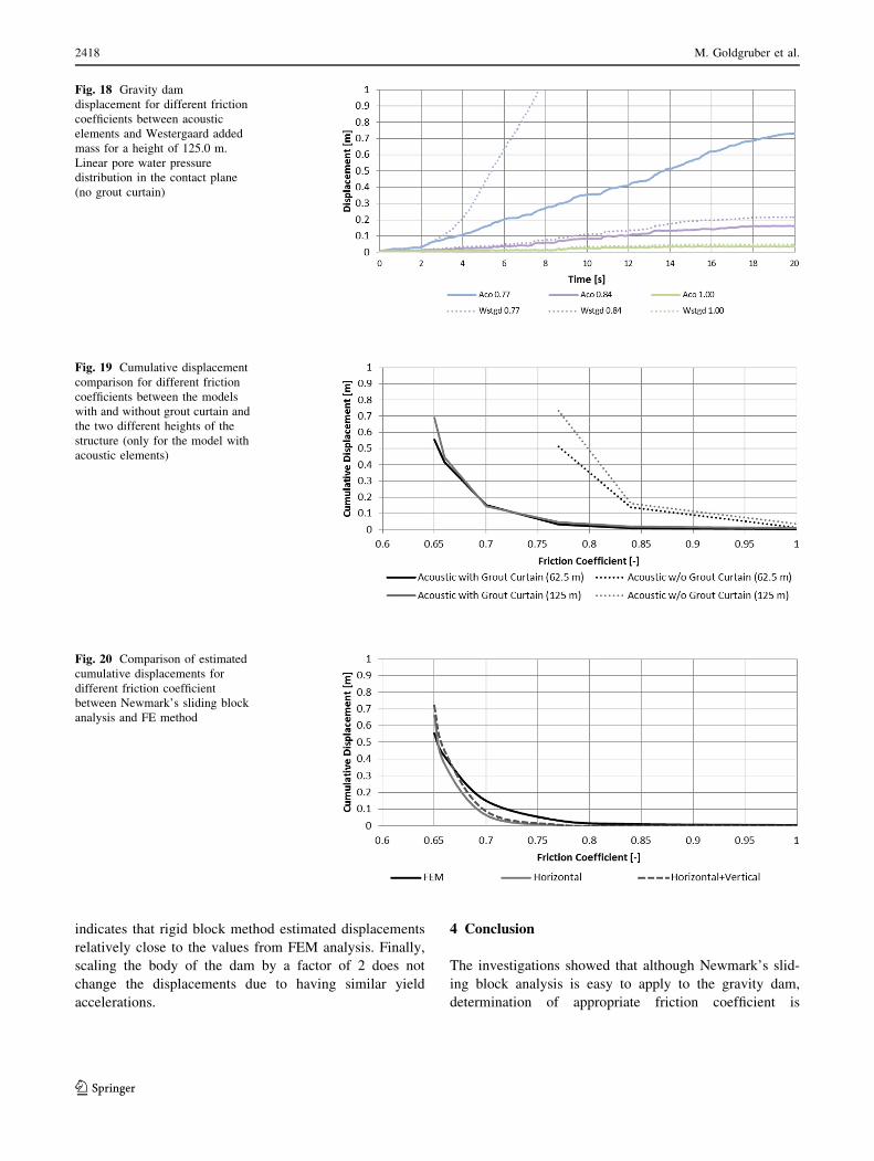
3.3 Results Comparison Between Newmark’s Sliding

Block Analysis and FEM

The cumulative displacements which were calculated with

the rigorous rigid block method are compared with those

calculated by the finite element method for different fric-

tion coefficients (Fig. 20). Including vertical acceleration

in the rigid block method increased the cumulative dis-

placements by increasing sliding phases. Furthermore, the

analysis which takes into account the flexibility of the dam

(FEM) shows higher sliding displacements for friction

coefficient between 0.66 and 0.77. Comparison of cumu-

lative displacements for higher friction angles (ls C 0.77)

Fig. 15 Gravity dam

displacement for different friction

coefficients between acoustic

elements and Westergaard added

mass for a height of 125.0 m

Fig. 16 Cumulative displacement

comparison for different friction

coefficients between the models

with acoustic elements,

Westergaard added mass and the

two different heights of the

structure

Fig. 17 Gravity dam

displacement for different friction

coefficients between acoustic

elements and Westergaard added

mass for a height of 62.5 m.

Linear pore water pressure

distribution in the contact plane

(no grout curtain)

Dynamic Sliding Analysis of a Gravity 2417

123

indicates that rigid block method estimated displacements

relatively close to the values from FEM analysis. Finally,

scaling the body of the dam by a factor of 2 does not

change the displacements due to having similar yield

accelerations.

4 Conclusion

The investigations showed that although Newmark’s slid-

ing block analysis is easy to apply to the gravity dam,

determination of appropriate friction coefficient is

Fig. 18 Gravity dam

displacement for different friction

coefficients between acoustic

elements and Westergaard added

mass for a height of 125.0 m.

Linear pore water pressure

distribution in the contact plane

(no grout curtain)

Fig. 20 Comparison of estimated

cumulative displacements for

different friction coefficient

between Newmark’s sliding block

analysis and FE method

Fig. 19 Cumulative displacement

comparison for different friction

coefficients between the models

with and without grout curtain and

the two different heights of the

structure (only for the model with

acoustic elements)

2418 M. Goldgruber et al.

123

complicated for the dam and foundation interface. Because

very small changes in friction coefficients can lead to very

large differences in displacements. The other key element

in this analysis is choosing appropriate ground motion

records. Choosing a ground motion record with low peak

value can lead to underestimation of the displacements.

Further investigation is required for choosing appropriate

friction coefficient and earthquake records.

Comparison of empirical regression equations and rig-

orous Newmark analysis has shown that in this study, the

Jibson98 equation can estimate the sliding displacements

for low friction coefficients (ls B 0.77) fairly close to

those from the rigorous sliding block. The problem with the

empirical formulas is that the user can not include vertical

acceleration in the calculation of the cumulative

displacements.

The investigation of the problem with the numerical

method showed that different modelling techniques of the

reservoir do not have a considerable impact on the results

of the displacement. The same applies also for different

heights of the structure if the friction coefficient does not

reach a low and critical value. Nevertheless, one should be

aware of the fact that this just holds for the relative dis-

placements between two parts, but can influence stresses,

velocities, accelerations, deformations, etc., significantly.

Having a look at the resultant displacements of the struc-

ture for different friction coefficients it is shown, that by

reaching a specific value, in this case 0.77 with and 0.84

without grout curtain, the displacement gets progressive.

Using the simplified formula of the Westergaard added

mass for such problems may lead to overestimated results,

wrong system behaviour and a divergent behaviour of the

numerical procedure. Contrary the use of the rigorous

formula did work out for simulations where the simplified

one failed to converge. Assuming a linear pore water

pressure states that the functionality of a grout curtain is a

prerequisite, because otherwise the structure may fail even

much faster. Nevertheless, in practice, the grout curtain

may crack and leak during a seismic event and therefore

the uplift will be increased. The assumed linear distribution

is a conservative approach in this case, because the pore

water pressure will not propagate like that in just a few

seconds of the earthquake.

The negligence of the cohesion in the simulations leads

to conservative results and a remaining safety margin;

however, it can be concluded that the failure of such a

structure will happen suddenly after reaching a specific

value of resistance.

Though this work is focused on the investigation of a

concrete dam, the proposed methods can also be applied on

problems regarding rock wedges in abutments of structures

interacting with surrounded water.

References

Ambraseys NN, Menu JM (1988) Earthquake-induced ground

displacements. Earthquake Eng Struct Dynam 16:985–1006

Arias A (1970) A measure of earthquake intensity. Seismic Design for

Nuclear Power Plants. Massachusetts Institute of Technology

Press, Cambridge, pp 438–483

Bundesministerium fur Land- und Forstwirtschaft (2001) Erdbeben-

berechnungen von Talsperren. Band 1, Grundlagen

Chopra AK, Hall JF (1982) Earthquake-induced base sliding of

concrete gravity dams. J Struct Eng 117:3698–3719

Dassault Systemes (2011) Abaqus 6.11-EF2 documentation. Dassault

systemes. Providence, USA

Goldgruber M, Shahriari S, Zenz G (2013) Influence of damping and

different interaction modelling on a high arch dam. Vienna

congress on recent advances in earthquake engineering and

structural dynamics, VEESD

Hilber HM, Hughes TJR, Taylor RL (1977) Improved numerical

dissipation for time integration algorithms in structural dynam-

ics. Earthquake Eng Struct Dynam 5:583–584

Housner GW (1954) Earthquake pressures on fluid containers. Report

EERL-1954-3, Earthquake Engineering Research Laboratory,

California Institute of Technology, Pasadena

Jibson RW (1993) Predicting earthquake-induced landslide displace-

ments using Newmark’s sliding block analysis. Transp Res Rec

1411:9–17

Jibson RW, Harp EL, Michael JM (1998) A method for producing

digital probabilistic seismic landslide hazard maps: an example

from the Los Angeles, California area. US Geological Survey

Open-File Report, pp 98–113

Lysmer J, Kuhlemeyer RL (1969) Finite dynamic model for infinite

media. J Eng Mech Div 95:859–876

Massachusetts Institute of Technology (1976), SIMQKE, A program

for artificial motion generation. Department of Civil Engineer-

ing, NISEE

McGuire RK (1974) Seismic Structural Response Risk Analysis,

Incorporating Peak Response Regressions on Earthquake Mag-

nitude and Distance. Massachusetts Institute of Technology,

Department of Civil Engineering, Research Report 74–51

Muto M, von Gersdorf N, Duron Z, Knarr M (2012) Effective

modelling of dam-reservoir interaction effects using acoustic

finite elements. 32nd annual USSD conference, innovative dam

and levee design and construction for sustainable water

management, pp 1161–1167

Newmark N (1965) Effects of earthquakes on dams and embank-

ments. Geotechnique 15:139–160

Selecting Seismic Parameters for Large Dams Guidelines (2010)

ICOLD, Bulletin 72, Revision 5.3.1

Westergaard HM (1933) Water pressure on dams during earthquakes.

Trans Am Soc Civ Eng 98:418–472

Dynamic Sliding Analysis of a Gravity 2419

123