Earnings Management and the Cost of Capital · It is clearly noted that account manipulation is...

2009 Erasmus University Rotterdam

Faculty: School of Economics. Section: Accounting, Audit & Control Name: Shaun A. Balvers (307621sb) Date: 20 August 2009 Instructor: E. A. de Knecht RA Co-Reader: Dr. sc. ind. A. H. v.d. Boom

[EARNINGS MANAGEMENT AND THE COST OF CAPITAL] The economic scientific literature contains much attention focusing on the incentives of the use of earnings management. This research will investigate whether firms manage earnings to profit from a lower cost of capital. Firms face two forms of cost for capital and two different parties, based on different assumptions, demand the rewards for capital. The cost of debt is the paid interest by the firm to the lenders. The payment for the cost of equity is the dividend payout of the firm. It is reasonable to understand that if a firm presents positive earnings, debt holders are less reluctant to grant a loan. One of the proxies used to determine the interest rate is the risk profile of the firm. The lower the risk profile the lower the interest rate. Concerning the cost of equity, investors qualify firms that produce steady earnings as less risky. Consequently based on this assumption, do investors require a lower payout, in reply to this lower risk? Is the cost of capital another incentive for managers to manage earnings?

Earnings Management and the Cost of Capital

Page 1

Table of Contents

1. Introduction .................................................................................................................................... 4

1.1.1 Research Question .......................................................................................................... 4

1.1.2 Literature......................................................................................................................... 5

1.1.3 Contributions .................................................................................................................. 5

1.1.4 Sample and Method ........................................................................................................ 6

1.1.5 Limitations ....................................................................................................................... 6

1.1.6 Structure ......................................................................................................................... 6

2 Earnings Management .................................................................................................................... 8

2.1 What is earnings management? ............................................................................................. 9

2.2 In which way are earnings managed? ................................................................................... 10

2.2.1 Account choice .............................................................................................................. 11

2.2.2 Activity manipulation .................................................................................................... 12

2.3 Why do firms engage in earnings management? ................................................................. 12

2.4 Summary ............................................................................................................................... 14

3 Cost of Capital ............................................................................................................................... 15

3.1 What is the content of the term the cost of capital? ........................................................... 15

3.2 What influences the cost of capital?..................................................................................... 16

3.3 The cost of capital structure ................................................................................................. 17

3.3.1 Cost of Equity ................................................................................................................ 17

3.3.2 Cost of Debt .................................................................................................................. 18

3.4 What is the relation between the use of earnings management and the cost of capital .... 19

3.4.1 Earnings (management) and risk .................................................................................. 20

3.5 Summary ............................................................................................................................... 20

4 Prior research and Hypothesis development ............................................................................... 22

4.1.1 Accrual models .............................................................................................................. 22

4.1.2 Industry model .............................................................................................................. 26


Page 2

4.1.3 Income smoothing ........................................................................................................ 26

4.2 Hypothesis Development ...................................................................................................... 26

4.2.1 Equity Capital ................................................................................................................ 27

4.2.2 Debt Capital ................................................................................................................... 27

4.2.3 Income smoothing ........................................................................................................ 28

4.3 Summery ............................................................................................................................... 28

5 Research Design ............................................................................................................................ 30

5.1 Research approach................................................................................................................ 30

5.2 Sample size ............................................................................................................................ 31

5.3 Method ................................................................................................................................. 31

5.3.1 Outcome variable .......................................................................................................... 32

5.3.2 Predictor variable .......................................................................................................... 34

5.3.3 Control Variables ........................................................................................................... 34

6 Empirical Research ........................................................................................................................ 37

6.1 Industry specific parameters................................................................................................. 37

6.2 Descriptive statistics ............................................................................................................. 39

6.2.1 Results from an uncontrolled model ............................................................................ 40

6.2.2 Results from controlled model ..................................................................................... 42

6.2.3 Industrial influence ....................................................................................................... 44

6.3 Results accrual approach ...................................................................................................... 46

6.3.1 Preliminary results ........................................................................................................ 46

6.3.2 Generalization ............................................................................................................... 47

6.4 Hypotheses results and Summary ........................................................................................ 48

7 Conclusion ..................................................................................................................................... 50

7.1 Conclusions and Limitations ................................................................................................. 50

7.1.1 Earnings management and the cost of equity .............................................................. 50

7.1.2 Earnings management and the cost of debt ................................................................. 51

7.2 Further research ................................................................................................................... 51


Page 3

Bibliography .......................................................................................................................................... 53

Appendix ............................................................................................................................................... 56


Page 4

1. Introduction

Earnings management for decades has been a subject of discussion, modern definitions of earning

management going back to 19871. Since then studies have been carried out to explain incentives for

the use of earnings management. It is clear; earnings management is a complicated subject that is

not caused by one or two incentives.

It is clearly noted that account manipulation is frowned upon; however detecting it is not easy. The

following citation presents a good explanation for earnings management.

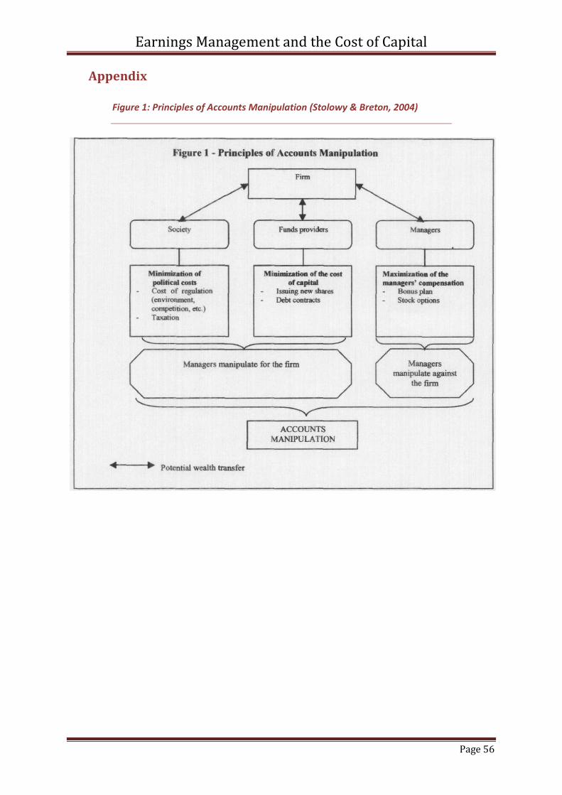
“Accounts manipulation is defined at the use of management’s discretion to make accounting

choices or design transactions so as to affect the possibilities of wealth transfer...”(Stolowy &

Breton, 2004, p. 6)

The focus on the definition of earnings management is irrelevant at this stage. Unlike most

definitions of earnings management, this quote states the possibilities of wealth transfer. Stolowy

and Breton continue to signal three forms of wealth transfer (Appendix, Figure 1).

“...wealth transfer between company and society (political costs), funds providers (cost of

capital) and managers (compensation plans).”(Stolowy & Breton, 2004, p. 6)

Studies that have been performed concerning earnings management often focus on either the

political cost or the cost of the managers, i.e. compensation costs. This research will investigate

whether or not firms manage earnings to profit from a lower cost of capital. Stakeholders use

accounting numbers in debt covenants; therefore, managers have an incentive to manage these

numbers (Beneish, 2001, p. 8). However, debt issuers are not the only parties that expect a return on

their invested capital. Besides an increased market value, investors also expect a cash return from

firms, in the form of a dividend.

1.1.1 Research Question

The purpose of this research is to provide better insight into the incentives that drive earnings

management. As explained before, earnings management is a complex term that has no clear

existence. Although most researchers agree that debt contracts are one of these incentives, they

focus their attention on the violation of debt covenants. This ex-post view of the issue assumes that

distributors of capital (i.e. equity or liabilities) have already assessed the firm’s risk, and calculated

the risk profile into their expected/ required payout. Debt covenant violations are based on existing

information. With expected earnings only being based on presumption, passed earnings presents an

indication for future profits.

1 Davidson, Stickney and Weil, cited by Beneish 2001


Page 5

This research will investigate whether a lower cost of capital has any influence on the managers’

incentives to manage earnings. Therefore, the research question is as follows:

Do managers of firms use earnings management to benefit from a lower cost of capital for the firm?

The research question is supported by two sub questions:

1. What is the content of term earnings management?

2. What is the content of the term cost of capital?

3. What is the relation between earnings management and the cost of capital?

With the explanation of these sub questions, the research question will be supported. The term

earnings management is a complex term. A scientific view on this subject will present greater

insights into the possible incentives that surround earnings management.

1.1.2 Literature

When researching the topic of the cost of capital, it is relevant to indicate that the cost of capital

exist in two forms, i.e. cost of equity and the cost of debt. Literature that researches the cost of debt

concerning earnings management is often ex-post. Dichev and Skinner (2000) investigate the

likelihood that manager’s choice accounting standards that best reduce the likelihood that their firm

will violate debt covenants.

The issue on the cost of capital is also well documented. Yet, authors seem to either look at

accounting choice, more often seem to investigate the quality or the quantity of disclosures (Francis,

Nanda, & Olsson, 2008). It is assumed that earnings announcements are a form of disclosure. This is

not far from the truth, as earnings are part of a very important aspect of the firm’s disclosure to

stakeholders. Concerning the use of earnings management, accounting choice is perceived as one of

the tools managers employ to manage earnings. However, conventional models used for exploring

the possibility of earnings management are discretionary accrual models.

1.1.3 Contributions

This topic is interesting for a number of reasons. Firstly, within the accounting and audit profession

this subject also reflects the usefulness of reported information. If firms report information that can

be manipulated, then how useful is the information. Misleading financial reports negatively affect

allocation resources (Healy & Wahlen, A Review of the earnings management literature, 1999). Audit

reports are designed to add value to the publicized information. However audit technology is

imperfect (Ronen, Tzur, & Yaari, 2006) and managers can move within the boundaries set by


Page 6

regulators. Nonetheless, auditors should be aware of the incentive by mangers. It is apparent that

stakeholders regard the information as useful and reliable.

Furthermore, from an academic point of view, both subjects (the use of earnings management and

the cost of capital) have been well researched. Papers investigating the use of earnings

management, assume that earnings management only harms the interest of the firm. However,

mangers that manipulate accounts to achieve a better (lower) cost of capital benefit the firm.

According to Watts and Zimmerman (1978), this is one of the two cases2 in which the firm benefits

by managers manipulating earnings(Stolowy & Breton, 2004). Most researchers agree that debt

covenant violations are an incentive for managers to manipulate earnings. However, they assume

that the debt has been granted. Is it not plausible that lenders assess the risk of lending capital, and

process this risk in the desired interest rate?

1.1.4 Sample and Method

This research will use Dutch stock exchange quoted firms on the EuroNext Amsterdam. The top 50

firms of the Amsterdam EuroNext are noted in the Amsterdam Exchange Index (AEX) and in the

Amsterdam Midcap Index (AMX). Preceding researches focus their research on the firms in the

United States. The dependant variable will be the use of earnings management. To detect a

possibility of earnings management the Modified Jones model (Dechow, Sloan, & Sweeney, 1995)

will be used. For the independent variable, the focus will be on the cost of capital. Two costs aspects

will be considered, i.e. the cost of equity and the cost of debt.

1.1.5 Limitations

The data selected comes from the Dutch stock exchange. Therefore, they represent the situation in

the Netherlands. Due to the difference in law, the outcome may not be applicable for global

application. However, cross-country analysis could take place to evaluate differences. Further

limitations include the data availability. As dividend is need as a variable to calculate the cost of

equity, firms that do not structurally release dividend will be excluded. However, firms that

periodically neglect to pay dividend sporadically, will remain included.

1.1.6 Structure

The structure of this paper will continue as follows. Chapters two and three will give a literature

review on the subject earnings management and the cost of capital, respectively. In chapter four the

relationship between the two main elements will be discussed. Prior research and the hypothesis

development will be addressed in chapter five. In chapter six the complete research design will be

2 Stolowy and Berton (2004) use the three aspects that were created by Watts and Zimmerman (1978) in stating their definition of account manipulation (Appendix, figure 1). Therefore, the other case in which earnings manage benefits the firm is when it affects society (Political costs). According to Watts and Zimmerman (1978) only compensation plans to managers, act against the best will of the firm.


Page 7

given, paying attention to the type of research, the method for testing, variables, control variables

and data sampling. In chapter seven the result from the research will be presented. The limitations

and recommendation will be laid out in chapter eight, ending with the conclusion.


Page 8

2 Earnings Management

This chapter contains, background information concerning the use of earnings management.

Paragraph 2.1 elaborates on the content of the term earnings management and describes what

earnings management implies. Paragraph 2.2 comments in which way earnings are managed. Firms

have different ways of managing earnings. Activity manipulation as a form of earnings management

will also briefly be commented on. The last paragraph will investigate why firms engage in earnings

management and what incentives exist for the use of earnings management.

Inefficient Market

Throughout this paper, the asymmetric information gap between the principal and the agent is

noted. This supports the notion that markets are not efficient in the strong form3. According to the

Efficient Market Theory (EMT), the strong form states that all information (public and private) are

included in the market price. This entails that insider information (e.g. information known to

management) is reflected in the share price. If this were true, reported information would not affect

the stock price, as the stock price would already reflect this information. The incentive for

management to manipulate earnings would be void. If managers reported manipulated earnings and

the market was efficient in the strong form, investors would not be deceived. Managers would

therefore not be able to manipulate the capital markets. (Levy & Post, 2004)

Earnings management

In the light of past accounting scandals and the current world economics, the credit crunch, the

subject of the use of earnings management has been receiving great attention. In 2001, the

investment world was shocked when the smartest guys in the room4 were caught manipulating

accounts. The Enron affair bought to daylight the significant effects of earnings manipulation.

Unfortunately, the Enron affair does not stand on its own. Since 2002 there has been a number of

accounting scandal were earnings have been overstated (e.g. Royal Ahold, Parmalat and more

recently Satyam Computer Services).

It is not always clear when firms operate outside the boundaries set by regulators. However, a fine

line exists between earnings management and fraud. The definition of fraud is “one or more

intentional acts designed to deceive other persons and cause them financial loss” (National

Association of Certified Fraud Examiners, 1993, p. 6). Within the economic scientific literature, fraud

3 The three forms of the Efficient Market Theory (EMT) are, the weak form, the semi-strong form and the strong form. In the weak form, only historical data reflects the price of a share. In the semi-strong form, all relevant public information is reflected in the share price. The strong form states that all information (public and private) is reflected in the stock prices (Levy & Post, 2004).

4 A documentary about the Enron corporation, its faulty and corrupt business practices


Page 9

is considered as moving outside the boundaries that have been set by standard setters. Earnings

management on the other hand, is misleading users based on an optimistic or a pessimistic bias by

managers (Vander Bauwhede, 2003, p. 197). Managers that operate outside the boundaries set by

regulators, reveal a corrupt view on the issue. However, earnings management operates more often

than not within the guidelines set by the reporting authorities. Standard setters have granted

managers a certain degree of discretion in reporting financial information. This is granted to allow

managers to reflect information only know within the firm, which is of value to outsiders (Palepu,

Healy, Bernard, & Peek, 2007, p. 7). It is this form of earnings management that will be considered

throughout this paper.

2.1 What is earnings management?

Healy and Wahlen (1999) state earnings management as follows:

“Earnings management occurs when managers use judgment in financial reporting and in

structuring transactions to alter financial reports to either mislead some stakeholders about

the underlying economic performance of the company or to influence contractual outcomes

that depend on reported accounting numbers.” (Healy & Wahlen, A Review of the earnings

management literature, 1999, p. 368)

In this definition, Healy and Wahlen state a judgement criterion, as well as the goal of the use of

earnings management.

The judgement criterion implies that earnings management is an activity that is purposely

undertaken by the management. This judgement criterion is cited in a number of articles as moving

within the boundaries set by regulators (e.g. (Daniel, Denis, & Narveen, 2008, p. 4) and (Beneish,

2001, p. 3)). This criterion implies that the management does not intentionally manipulate accounts.

However, it implies the use of professional discernment used by management and granted by

authorities. This discernment addresses the main challenge researches face (Beneish, 2001, p. 3).

Graham et al. (2005, p. 5) notes however, that in the “post-Enron environment”, managers are

reluctant to utilize the liberty presented to them to create adjustments within accounting

standards5. According to Bergstresser and Philoppon (2006, p. 514), earnings management arises,

when reported income includes cash flows and changes in the firm value. Since cash flows are not

difficult to establish and trace, changes in the firm value requires a greater deal of management

discernment.

5 Since the Enron case, the U.S. government past the Sarbanes-Oxley Act. Violation of this act can result in 20- year imprisonment and a monetary fine.


Page 10

Healy and Wahlen also state the goal for the use of earnings management. On the one hand

misleading stakeholders, and on the other hand influencing contractual outcomes. In general,

earnings management is aimed at wealth transfer (Stolowy & Breton, 2004).

2.2 In which way are earnings managed?

Financial reports convey earnings that have occurred throughout the past period. These earnings are

based on cash flow plus changes in the firm value (Bergstresser & Philippon, 2006, p. 514). Whilst

cash flows are easily determined, changes in the firm value are more challenging. It is in determining

this change in the firm value that managers are granted some slack by standard setters. Cash flows

(cash accounting) are easily measured and defined. However, they fail to reflect the complete value

change needed in periodic reports. To reflect the true change in the firm value, accrual accounting is

implemented. Common accounts used to manipulate earnings are the accrual accounts. The accrual

account is a product, designed by standard setters, to express valuation changes that have not yet

resulted in cash flows(Gao & Shrieves, 2002, pp. 3-4). It is in these accounts, where earnings

management is likely to be used (Beneish, 2001, p. 3). However, the aim of the standard setters was

not to provide managers with a possibility for using earnings management, but to express a

professional judgement.

Not all accruals are inferior and superfluous, as they were created for specific purpose. This poses

the problem that not all the accruals are related to earnings management. Non-discretionary

accruals are based on expectations from management and are determined based on subjective

assumptions. An unwarranted bias when determining accruals, leads to the use of earnings

management. The last form of accruals is considered the discretionary component and relevant to

earnings management (Beneish, Earnings Management: A Perspective, 2001, p. 3).

All firms, based on their sales and assets, are expected to have a certain level of accruals (Vander

Bauwhede, 2003). However when these accruals exceed non-discretionary levels, they could indicate

an inclination to manage earnings.

Methods

Over the years, to detect the use of earnings management, a number of methods have been

developed. Healy (1985) and DeAngelo (1986)6 developed methods that were very dependent on

years where no earnings management was suspected. That was the biggest weakness in these

models. They would expect discretionary accruals to be revealed in the difference between accruals

in a year where earnings had been managed and a year where no earnings management had been

suspected(Vander Bauwhede, 2003, pp. 198-199).

6 Cited from Vander Bauwhede (2003, p. 199)


Page 11

The Jones model (Jones, 1991) and the modified Jones model (Dechow, Sloan, & Sweeney, 1995)

were created to try eliminate the discretionary element of the accruals, by taking into consideration

changes in the economic environment (Beneish, 2001). However, like most models these models

have various limitations. Further elaboration will be noted in chapter five, prior research. Studies

have also shown that changes in inventory and in accounts receivables can resemble earnings

manipulation(Roychowdhury, 2006; Stolowy & Breton, 2004).

Rational minds would suggest that investors, being able to detect the use of earnings management,

would punish firms that violate the freedom granted to them by the standard setters. Studies

performed by Teoh Welch and Wong (1998b) and Teoh and Wong(2002) suggest that investors are

“naïve” in detecting earnings manipulations, due to the asymmetric information gap. Although

models exist that can predict the possibilities of the use of earnings management, an accurate

forecast remains difficult.

It should be noted, that most of the performed researches assume that the market is not aware of

the tendency by managers to alter the earnings. However according to a study by Stein (1989)

investors rationally expect managers to manage the earnings. Consequently in pricing stocks,

analysts expect managers to inflate earnings. The market knowingly cannot prevent this from

happening so anticipates this behaviour and expects earnings that have been managed (Cheng &

Warfield, 2005). This would be consistent with the efficient market assumption. The share price

reflexes all information, i.e. public and private. The share price therefore portrays a true view of the

firm, where managed earnings are processed in the market price.

Coles et al. (2006) suggest that investors are well informed and sophisticated in their awareness of

earnings deception. Nevertheless, the transparency into incentives and account manipulation is

limited. Even though models might be available, these models face limitations and can only indicate

the possible use of earnings management.

2.2.1 Account choice

Earnings management by means of accruals, seem to invoke a thought that last minute accruals are

only used once the result is known. When figures disappoint income inflating accruals are formed,

and when figures over satisfy expectation, income deflating accruals are used. However, research

exists suggesting that managers do not only use the slack presented to them by the standard setters

to create accruals. To evaluate the firm value, the standard setters require mangers to choose

appropriate accounting policies to valuate firm value. Research by Skinner (1993, p. 408) concludes

that highly levered firms have a bigger chance in choosing favourable accounting policies that

increased income. This could also be concluded when considering accounting-based bonus plans.

Initial studies focussing on account policies suggest that, firms systematically choose favourable


Page 12

accounting policies7(Vander Bauwhede, 2003, p. 198). The standard setters try to reduce the effect

policy changes incur in accounting figures. Auditors should also be aware of the inclination of

management to change accounting policies. Although firms have the possibility to alter policies, one

might suggest that investors would punish firms that too frequently change their accounting policies.

2.2.2 Activity manipulation

The most performed studies focus on account manipulation, however Roychowdhury (2006) suggest

that in comparison to activity manipulation, the effects of direct account manipulation are relatively

lower. The former is characterized by a deviation from the normal operation with the primary

objective to meet certain earnings thresholds (Roychowdhury, 2006). One might argue that activities

that increase earnings are only good for the firm. Roychowdhury notes an increase in sales by means

of temporary discounts. This certainly cannot harm the interest of the firm. Investors might

appreciate a certain degree of entrepreneurship to meet earnings targets, given that long-term

objectives are not jeopardized. However, earnings manipulation is notorious for its short-term

interests. Managers manipulate earnings to mislead investors and benefit from the wealth transfer

between investors and management (Stolowy & Breton, 2004). Activity manipulation does not

support this notion, because it does not mislead investors. Reported earnings by management are

correctly stated, and do not present an untrue view of the value of the company. In the core,

earnings management through account manipulation does not always materialize and produce cash

flows, therefore not benefiting investors. Cash flows alter the capacity of firms to pay out dividend.

DeAngelo and DeAngelo (2006a) research suggests that dividend payouts are important to investors.

Further research has shown that dividend cuts are unforgiving punished at the stock market (Pettit,

1972; Aharony & Swary, 1980; Grullon, Michaely, & Swaminathan, 2002). Therefore earnings that do

not materialise into cash flow, damage the cash position of the firm.

2.3 Why do firms engage in earnings management?

Although throughout the economic significant literature, different incentives have been presented

regarding the existence of earnings management, Stolowy and Berton (2004) state that the use of

earnings management exists to profit from the possibilities of wealth transfer. Beneish (2001)

distinguished between four possible motives for earnings management.

1. Debt contracts;

2. Compensation Agreements;

3. Equity Offerings;

4. Insider trading.

7 Examples of favourable accounting policies are activating expense and depreciating them in year to come.


Page 13

Debt covenants often use accounting information to regulate firms’ performance and incorporated

dividend restrictions in them(Bradley & Roberts, 2004)8. Cash flows that exit the firm in a form of

dividend, weaken the position of the debt providers. When earnings fall short of dividend levels (i.e.

income is greater than the proposed dividend), constraints within debt contracts restrict payout

(Daniel, Denis, & Narveen, 2008, p. 3). Beneish (2001, p. 8) summarizes studies that reveal mixed

results for the use of earnings management to avoid defaults on loans. The main objection of using

earnings management to influence debt covenants’ is that it is not clear if these actions postpone

the inevitable. Do firms that apply earning management to avoid defaults, eventually default?

Although some firms may not default on their loans, they profit from a relatively cheap form of

capital (Stolowy & Breton, 2004, p. 6). Due to higher earnings, companies could seem more

profitable than in reality. This subject will be addressed more in depth in the next chapter.

Compensation contracts seem to provide more evidence for the existence of earnings management

than debt contract. Extensive studies (e.g. (Bergstresser & Philippon, 2006; Bauman & Shaw, 2006;

Ronen, Tzur, & Yaari, 2006; Healy, 1985)) have shown that in general the self-interest motivation of

management is a great incentive using earnings management, than that of the debt covenants.

Managers receive compensation based on their performance. The compensation theory is based on

the agency theory. The principal (stakeholders) and the agent (management) both want to increase

their wealth. The principal can align the two incentives by increasing the wealth of the agent, when

his own wealth increases. However, not all performance indicators are financial and quantitative.

Creating uncomplicated, unbiased and clear performance indicators is not easy. Consequently, most

performance indicators are financial figures. In a Towers Perrin survey, 65 of the 68 sample

companies using single performance measurement used accounting indicators as performance

measurement. 62% of the selected companies using multiple performance measurements used

accounting indicators. Performance can be measured in a number of ways from total earnings to

growth rates9.

Equity offerings offer a great opportunity to manage earnings. Due to the information asymmetry,

managers are known to inflate earnings to receive a better price for new equity (Beneish, 2001). This

is consistent with the notion that management aspire to receive a relatively low cost of capital.10

Rangan(1998); Teoh, Wong and Rao(1998); and Teoh et al.(1998a; 1998b) have performed extensive

8 In a research performed by Bradley and Robert (2004), they found that a great majority (84%) of all private debt contracts have dividend restrictions

9 Cited from (van Winsen, 2008)

10 If the cost of equity (CoE) is measured by 𝐶𝑜𝐸 =

𝐷𝑖𝑣𝑖𝑑𝑒𝑛𝑑

𝐸𝑞𝑢𝑡𝑖𝑦. A larger denominator will reduce CoE, ceteris

paribus.


Page 14

studies into earnings management and equity offerings. Their evidence suggests that earnings are

managed before equity offerings subsequently disappoint expectations.

Insider trading has also been documented (Beneish, Earnings Management: A Perspective, 2001),

(Ronen, Tzur, & Yaari, 2006), however the evidence supplied is less persuasive. Insider trading could

be regarded as a form of management compensation. Management receives equity compensation

throughout the years. However, knowing the true state of the firm, managers have more incentive

to cash in holdings when they know the firm is overstated (Beneish, 1999). Beneish(2001, p. 10) even

argues: “If managers act as informed traders, I expect them to use their information about earnings

overstatement to trade for their own benefit...”. (Ronen, Tzur, & Yaari, 2006, p. 362) study supports

recommendation to ban insider trading.

2.4 Summary

In this chapter, the term earnings management was discussed. From the definition presented, it is

clear that the use of earnings management differs from fraud. The former being considered over

optimism instead of outright disregard for accounting standards. Furthermore, the difference forms

of earnings management were noted. This paper will focus on the accrual method. However, activity

manipulation and account manipulation were also stated as possibilities for earnings management.

The last paragraph in this chapter, states the reasons why firms or managers engage in earnings

management. Four distinctive reasons were noted, i.e. debt contracts, compensation agreements,

Equity offerings and insider trading.

The next chapter will focus on an issue that derives from debt contract. Although the cost of capital

is not only limited to debt contracts, it is certainly a term that is related to capital agreements. The

content of the cost of capital is outlined in the next chapter.


Page 15

3 Cost of Capital

In the previous chapter, the content of the term earnings management has been examined. This

term derives its existence from accounting principles. The cost of capital, however, is more often

used within finance related subjects. Every firm faces some sort of capital cost. In this chapter, a

literature overview will be presented of the cost of capital. In the first section, a definition will be

supplied about the content of this term. In the second section, an overview will be presented

concerning the issues that influence the cost of capital. A quick examination will be provided

concerning the issues relevant to this study. In the final section of the paragraph, the cost of capital

will be further explained in a more direct approach. The two elements that create the total cost of

capital will be addressed. The chapter will end with a summary of the commented issues.

3.1 What is the content of the term the cost of capital?

Essentially, the cost of capital is the price a firm pays for the use of capital. However, this is not the

only purpose the cost of capital has for a firm. Modern corporate decisions are based on the rate at

which a firm is able to attract capital from the capital markets. Investment decisions are made and

cash flows discounted based on the weight average cost of capital(Easley & O'Hara, 2004, p. 1553).

Capital that firms hold are debt or shareholders equity, the costs are respectively interest and

dividend. However the price of these forms of capital differs in that, generally the costs of debt are

lower than that of equity. The greatest primary reason for this difference is that, the risk debt

distributors are exposed to are inferior to that of equity distributors. In other words, the amount of

risk an investor is willing to take depicts the return he expects to make. Modern finance theories

associate return with the risk profile of an investment product. The Capital Assets Pricing Model

(CAPM)11 calculates the expected return rate of a portfolio based on the risk profile in relation to the

market risk. This model is a classic portrayal of the relationship between the risk of an investment

product and the expected return.

Investors have a different return on investment than the firms cost of capital, subsequently investors

can also achieve a change in the market value whilst a firm only pays its dividend or interest.

However, a clear relation exists between the risk of doing business and the returns it presents. Risk

is influenced by numerous factors. For this research, the focus will mainly be on the information risk.

Information risk.

The agency theory is the foundation behind the information risk. An information gap exists between

the agent and principle. The principal requires the agent, being well informed, to reduce this gap.

11

The CAPM states that the sum of the market risk premium 𝑟𝑚 − 𝑟𝑓 , sensitive to market movements 𝛽𝑖

and the risk free premium 𝑟 can estimate the expected return on a well-diversified investment portfolio. (Brealey, Myers, & Allen, 2006, p. 189)


Page 16

However, the principal cannot judge the quality of the conveyed information. Francis et al. (2005, p.

296) defines the information risk as follows:

“... the likelihood that firm specific information that is pertinent to investor pricing decisions is

of poor quality.”

Within the finance theory, risk has two components, i.e. systematic risk and specific risk. The former

is non-diversifiable and is inherent to investments in general. The latter is diversifiable and can be

eliminated by a well-diversified portfolio12(Brealey, Myers, & Allen, 2006, pp. 147-181). A number of

researches that have shown that information risk is a part of the non-diversifiable risk factor(Easley

& O'Hara, 2004; Francis, LaFond, Olsson, & Schipper, 2005). As a result, diversification will not

eliminate the information risk, and classifying the information risk as a price risk factor(Francis,

LaFond, Olsson, & Schipper, 2005, p. 296). Therefore when engaging in investments, the information

risk is firm specific and not a general risk taken. Being a firm specific risk, the information risk differs

per firm. Investors have great advantages in identifying this risk. According to the definition provided

by Francis et al. (2005), the information risk exists when information (disclosure) is of poor quality.

Arther Levitt, chairman of the Security and Exchange Commission, stated that:

“Quality information is the lifeblood of strong vibrant markets. Without it, ... Fair and efficient

markets cease to exist.”(Levitt, 2000)13

The quality of the disclosure is dependent on many aspects. Yet modern pricing models do not take

the information issue into account(Easley & O'Hara, 2004).

3.2 What influences the cost of capital?

The cost of capital is a reflection of the risk that is taken by the investor. As stated before, a part of

this risk is the information risk. Francis et al. (2005) has provided empirical support that information

risk is associated with the cost of capital. Furthermore, Easley and O’Hara (2004) investigate the role

of the private and the public information in determining the cost of capital. Two aspects are mainly

associated with the information risk. Francis et al. (2008) investigates the influence of voluntary

disclosure and the earnings quality, the latter being prodominantly driven by the accural quality14.

Two different predictions are noted with regards to the earning quality and the disclosure published

by a firm, i.e. a substitutive and a complementary connection (Francis, Nanda, & Olsson, 2008).

12

H. Markowitz was one of pioneers of the portfolio. His work proved that portfolio selection could reduce the standard deviation (risk) of an investment. His work has proved to be the cornerstone of modern risk-return relationships.

13 Cited from: (Easley & O'Hara, 2004), speech: (Levitt, 2000)

14 Francis et al. (2008) mentions three measures in establishing earnings quality, i.e. accrual quality, earnings variability and the absolute value of abnormal accruals.


Page 17

However, it is not certain which one of these aspects are th emost essential in determining the cost

of capital. On the one hand, research performed by Diamond and Verrecchia(1991) suggests that

greater disclosure results in lower information risk and therefore in a lower payoff. On the other

hand, Kim and Verrecchia(1995) researched that greater disclosure results in even greater

information assymetry, leading to an increase in the expeceted payoff. This owing to an increase in

the assymetric information gap that new information can create. These two effects counterbalance

each other and lead to an aggregated payoff. Likewise, accruals produce both a possitive (true

performance measures) as well as a negative signal (over optimism). These effects both existing

simultaneously and producing an average cost of capital(Francis, LaFond, Olsson, & Schipper, 2005,

p. 296).

3.3 The cost of capital structure

The capital structure of the firm has become an important issue, since the publication of the

theorem develop by F. Modigliani and M. Miller (M&M)15. As indicated before, generally debt is

relatively less expensive than equity. Before the notion on M&M, debt was regarded as unavoidable.

The cost of debt, interest, was regarded as a cost. Yet, under the proposals published by M&M, no

sense existed in managing a firm’s capital structure. This notion is however, based on a world

without taxes and transaction costs. Once these elements are added to the equation, the capital

structure is an important issue, creating possibilities for firms to benefit from their capital structure.

Firms are however restricted in their capital ratio. Debt holders are sceptical towards excessive

unfavourable debt-equity ratios.

Although equity holders and debt holders both receive returns from the firms, between the two

groups a shareholder-bondholder conflict exists (Wald, 1999, p. 194). Bradley and Roberts (2004)

researched debt contracts, and found that a great majority stated dividend restrictions. These

restrictions are intended to eliminate possible wealth transfers between debt holders and equity

holders. In a research performed by Wald(1999), dividend restrictions are intended to maximize firm

value, and not the value of equity. Without these restrictions, possible debt holders would not grant

firms debt, as firms would prefer dividend payout to investing decisions (Wald, 1999, p. 195).

3.3.1 Cost of Equity

A firms cost of equity consists of a dividend payout. A study by Brav et al. (2005) showed that CFO’s

are willing to make great internal changes, from laying off personal to avoiding profitable projects,

just to avoid dividend cuts. DeAngelo and DeAngelo (2006a) concluded that dividends are vital to

investors, based upon negative share price reactions found around dividend cut announcements.

15

Modigliani and Miller, The Cost of Capital, Corporation Finance and the Theory of Investment, American Economic Review, 48 (June), pp.261-297


Page 18

The fact that equity holders do not always expect to receive a dividend, is shown in the fact that

some shares do not pay dividend. The share price accounts for a zero dividend payout. This is

however corporate strategy that is taken by the management. It is when investors expect a dividend

payout and are disappointed, that markets react with discontent. Dividend cuts alter expected

returns from investors. This last being one of the reasons the expected return on equity, thus the

cost of equity, is higher than that of debt. Equity holders risk the uncertainty that future profits will

not add (expected) value to holder’s investments. Moreover, cash flows from return on equity are

less certain. Debt holders also have a payout advantage, over equity holders. Interest is always

expensed, whereas dividend is reliant on positive (average) results. These two factors increase the

systematic risk (non-diversifiable risk) equity holders have above debt holders. Moreover, in the

event of discontinuity debt holders have a payment priority over equity holders. It is relevant to

state though, that in a case of discontinuity, debt holders are often deprived of any payback as well.

They run the same risks as equity holders, risking their initial participation. Why then would

investors want to hold firms equity? According to the CAPM, diversifiable portfolios are negatively

correlated to risks. The better the diversification the closer the correlation coefficient (𝜌)

approaches -1.

3.3.2 Cost of Debt

The realised cost of debt consists of interest payment. Studies have been carried out using the

marginal cost of debt(Prevost, Skousen, & Rao, 2008). Prevost et al. focus on corporate bonds, and

compare the yield spread on a corporate bond with that of a Treasury yield spread. This however

does not focus on the real interest expense of a firm. Prevost et al. (2008) does however contribute

to debt issued through bonds, reflecting accrual quality in the bond market. Bond market see

through manager’s intentions to inflate earnings, as higher marginal costs of debt are associated

with higher accruals (Prevost, Skousen, & Rao, 2008). Thus, the market expects a premium for

disclosure quality and for the information risk(Francis, LaFond, Olsson, & Schipper, 2005; Prevost,

Skousen, & Rao, 2008).

Although, equity holders are faced with specific risks that are inherent to their investment, debt

holders bear other risks. If debt being cheaper than equity, rational minds would suggest that firms

would, in a world with no restrictions, dump all equity and only take on debt. However, legislation

prohibits this and recently corporate statutes prevent this from happening(Wald, 1999, p. 195).

Moreover, if a firm only has equity, all risks are borne by the equity holders. Among these risks are

the risk of discontinuity and the risk of failing profits. When the firm take on debt, the first risk is

proportionally shared by all capital holders. The more debt a firm has the greater the proportion of

risk is shifted onto the debt holders. Considering the risk-return theory, debt holders would expect a

higher return. Nevertheless, firms aim for an optimal ratio between debt and equity. The optimal


Page 19

debt ratio in a firm is dependent on its production function16(Wald, 1999, p. 194). An optimal debt-

to-equity ratio would not only decrease capital costs, they would also achieve a lower weighted

average cost of capital (WACC17). Debt holders are also aware of the possibility of wealth transfer to

the equity holders, and impose restrictions on firms through debt covenants. In contradiction to

equity holders, once a covenant has been agreed upon, debt holder will have great difficulty

influencing firms operations.

Equity holders on the other hand, seem to appreciate a healthy capital structure and adopt

guidelines in corporate statues(Wald, 1999). Equity holders are aware of the payout advantage that

debt holders possess. However, debt confers advantages to equity holders. When taxes are included

in an M&M theorem, a firm increases it value by attracting debt. Greater firm value increases equity

holder’s value. Empirical research shows that firms with a lower debt-to-equity ratio are more

profitable, and have a respectively greater return on equity. In addition, those firms with a greater

credit rating and a lower cost of capital (Francis, LaFond, Olsson, & Schipper, 2005, p. 297).

3.4 What is the relation between the use of earnings management and the

cost of capital

Extensive testing exists concerning the use of earnings management. However, the majority of these

researches investigates the incentive schemes of manager’s as a cause for the use of earnings

management (e.g. (Gao & Shrieves, 2002; Ronen, Tzur, & Yaari, 2006; Bergstresser & Philippon,

2006)). This is just one of the explanations regarding the use of earnings management(Stolowy &

Breton, 2004, p. 6).

The primary reason concerning the use of earnings management is to influence the reported

earnings. A personal incentive for the management to manage earnings is the incentive schemes.

However, concerning the firm, the incentive is to reduce real expenses and maximize real profits (i.e.

cash flows). Research has been performed with regards to income increasing accounting policies

(e.g. (Skinner, 1993; Gietzmann & Ireland, 2005)).

In this paragraph, the relation between the use of earnings and risk will be described. The cost of

capital is derived from the risk related to an investment. Therefore, a negative association between

earnings and risk would depict a negative correlation between earnings and the cost of capital.

16

Production function portrays the optimal output (production) of a firm given its input. 17

𝑊𝐴𝐶𝐶 = 𝑟𝐷𝐷

𝑉+ 𝑟𝑒

𝐸

𝑉, where: 𝑟𝐷= return on debt, 𝑟𝐸= return on equity, D=Debt, E=Equity and V= Firm value

(Brealey, Myers, & Allen, 2006, p. 461)


Page 20

3.4.1 Earnings (management) and risk

In the previous paragraph, the relation between the risk of an investment product and the expected

return was explained. To calculate the risk18 (𝜎) of an investment, the standard deviation is

calculated between the expected return (𝑟 ) and the actual return (𝑟). Therefore earnings that fall

below the expected amounts, increase the risk. The previous chapter established that the cost of

capital, both debt as equity, are related to the risk of that an investment.

Smoothing

An earnings management strategy that has stood the test of time is income smoothing(Ronen &

Yaari, 2008, p. 319). Not all earnings management is aimed at achieving a maximum income.

Earnings benchmarks are often the cause of smoothed earnings. Graham et al.(2005, p. 20) mentions

that 51% of CFO’s regard earnings the most essential in reporting performance to stakeholders, and

not cash flows (Appendix, Figure 2). When earnings reach a certain level, excess earnings will not

return proportional stock movements. Bauman and Shaw(2006) mention that firms have even a

greater incentive to beat analysts forecast by small amounts. Cheng and Warfield (2005, p. 21) also

notice this event happening. Although they research earnings management towards management

incentive schemes, Cheng and Warfield note an important reason for the existence of smoothing

income19. Increasing income upwards constantly, is nearly impossible. However when income

reaches benchmark levels, residual earnings can be saved for future periods.

A survey carried out by Graham et al. (2005) asked managers why they preferred smooth earnings20.

The number one response (88,7%) was because investors perceive smooth earnings as less risky. A

great majority found that it reduced the return demanded by investors. Apparently, investors reduce

the risk premium built into the cost of equity and demand a low return when earnings are

smoothed. Graham et al.(2005, p. 5) further states rigorous stock movement when benchmarks are

missed, even slightly. Investors become weary when firms are unable to reach targets. Moreover,

investors’ associate benchmark misses with firms that are incapable of predicting their own future.

3.5 Summary

The capital position of the firm is essential. Although Modigliani and Miller first stated that, the

structure of a firm did not matter, when taxes and other impurities are added, capital structure

18 𝜎 =

1

𝑁−1 (𝑟 − 𝑟)2𝑁𝑡=1 , where

1

𝑁−1 represents the degree of freedom; 𝑁 is number of observations and 𝑡

the number of periods. (Brealey, Myers, & Allen, 2006, p. 156) 19

Cheng and Warfield note two issues. Only one is relevant to this paper. However Cheng and Warfield note that the second issue is that incentive contracts recurring and managers care about stock prices in the future (Cheng & Warfield, 2005, p. 21).

20 Appendix Table 1 gives an overview of the result to the question: “Rank the three most important measures report to outsiders”.


Page 21

matters. The costs for the different causes of capital are essential for this difference. The cost of

capital is driven by the risks that are taken. In diverse finance model, return is related to the risk

taken. CAPM states that some risks are diversifiable (specific risk) by means of a well divers portfolio,

but that a non-diversifiable (systematic risk) component still exists. Information risk is a systematic

risk, and consequently that risk is non-diversifiable. Francis (2005) states that with regards to the

information risk both voluntary disclosure and earnings quality are essential.

Furthermore, the cost of capital consists of the cost of debt and the cost of equity. These two forms

of cost differ, due to the different risks the holders face. The cost of debt is driven by the amount of

risk that the equity holders transfer to the debt holders. In turn, the equity holders also transfer

profits (interest expense) to the debt holders.

A firm faces many risks in doing business. However, the performance risk could be considered the

biggest of them all. According to modern finance theory, the standard deviation from the expected

return and the actual return is the risk. Therefore if a firm deviates from their expected returns, they

increase their risks. With a firms risk increasing, capital owners expect high returns. Earnings that

fluctuate too much are complicated in predicting future earnings. For research, it is possible to state

that smoothed earnings are considered less risky than high fluctuating earnings. To avoid a firm’s

risk profile increasing, mangers have the incentive to manger their earnings. This would not only

decrease the risk profile, but also improve net profits.

In the next paragraph methods developed of the past decade that detect the possible use of

earnings management, will be discussed. Furthermore, a number of hypotheses are derived that will

be the tested in following chapters.


Page 22

4 Prior research and Hypothesis development

In Chapter 2, the definition of earnings management was simplified as the difference between the

cash flow from operations (CFO) and the reported income(Bergstresser & Philippon, 2006, p. 514;

Vander Bauwhede, 2003, p. 198). Although the definition of Healy and Wahlen (1999, p. 368) is more

comprehensive, Bergstresser and Philippon highlight one of the aspects of earnings management,

i.e. accrual reporting21. Standard setters allow the use of accruals to improve reporting. Static

reporting standards hamper real valuation of assets and liabilities. Therefore, the use of accruals

allows management to provide vital information that could otherwise be lost in static reporting

standards. Accruals that distort reporting quality are known as discretionary accruals. The size of

these accruals is a benchmark for the use of earnings management.

In this chapter, prior research that has been developed over the years will be explained. An overview

is presented of developments into accruals based models. The chapter will furthermore, present the

developed hypotheses that are derived from existing economics scientific literature.

Cash flow versus earnings.

Fundamentally, firm value is based on discounting future cash flows. If a firm can produce a certain

output in the past, the output in the future should either be the same or preferably increase.

Consequently, the present cash flow is important. However, if cash flows do not contain the true

firm performance, can they still reliably be used for valuation purposes for a firm? The income

statement is used to portray periodic fluctuations in firm value. Firm value is more than net cash

flows, as some firm value is not yet recognized in the current cash flow(Bergstresser & Philippon,

2006, p. 514). They are however, part of the change in firm value. These changes are recorded in

accruals. Accruals that represent true value adjustments are non-discretionary (innate) accruals.

Determining these accruals is not always easy and require management’s expectations(Ronen &

Yaari, 2008, p. 320). When these expectations are unrealistic or unfounded, they create false value

to the firm. Specifically, value is created without the realistic expectation of future cash flows. These

types of accruals are regarded as discretionary accruals. Isolating this form of accruals is the

toughest challenge for researches(Beneish, 1999, p. 3)

4.1.1 Accrual models

Models that detect earnings management are continually evolving. The biggest contribution to the

accrual approach is the Jones model (Jones, 1991). However, in the first section a brief overview will

be presented into the development of the accrual model until Jones. Followed by a description of

21

Vander Bauwhede refers to two aspects that can be used to manage earnings, i.e. accrual studies and accounting method. The latter has more long lasting effects, as management cannot change accounting method annually. Therefore a preference for the former aspect. (Vander Bauwhede, 2003, p. 197)


Page 23

the Jones model (Jones, 1991) and the modification made to the model by Dechow et al. (1995),

known as the modified Jones model.

If accruals can be divided into two discretionary and non-discretionary components, the following

relation exists between these two components:

(4-1)

𝐷𝐴𝑡 = 𝑇𝐴𝑡 −𝑁𝐷𝐴𝑡

Where:

𝐷𝐴𝑡 Discretionary Accruals in year t

𝑇𝐴𝑡 Total Accruals in year t

𝑁𝐷𝐴𝑡 Non-Discretionary Accruals in year t

Equation 5-1 is the base of the assumptions throughout this paper. Based on the definition that

accruals are the difference between cash flow and earnings, the total accruals (TA) are calculated as

follows:

𝑇𝐴𝑡 = 𝐶𝐹𝑂𝑡 − 𝐸𝐵𝑋𝐼𝑡

Where:

𝐶𝐹𝑂𝑡 Cash flow from operations in year t

𝐸𝐵𝑋𝐼𝑡 Earnings before extra-ordinary income in year t

Pre- Jones models

The greatest difference between all the noted models, are their ability to isolate the discretionary

accruals. Only the total accruals are observable in financial statements, determining the

discretionary accruals are not straightforward. Accruals are either income increase (managed

upwards) or income decreasing (managed downwards). Healy (1985) states that over time accruals

are managed upwards and downwards. This creates an average accruals amount, which is equal to

the non-discretionary accruals. The Healy model calculates the non-discretionary component as

follows:

(4-2)

𝑁𝐷𝐴𝑡 =1

𝑛

𝑇𝐴𝑖𝐴𝑖−1

𝑛

𝑖=𝑡

Where:

𝐴𝑖−1 Lagged Assets in year t-1

𝑛 Total number of years in calculation


Page 24

In essence, Healy (1985) calculates the long-term average of the TA. Computing the NDA from the

average TA in equation 5.2, discretionary accruals were accruals that differ from the long-term

average total accruals (Equation 5.1).

Limitations to this method include the value of n. How many years in the past would be reasonable

to go back? When testing 𝑡 − 0, what would be a realistic value of 𝑛. Most research assumes that

n=5(Ronen & Yaari, 2008, p. 397). In addition, Healy’s model assumes that in comparison to assets,

innate accruals remain unchanged. Firm are expected to grow, over the years the composition of a

company could have changed. As innate accruals are a firm’s value outside of the present cash flow,

they are expected to grow with the firm. Moreover, accruals are controlled by the total assets.

Knowledge based firms use in general less assets. This causes the control variable of assets to

become less accurate(Stolowy & Breton, 2004, p. 22).

DeAngelo (1986) tried to simplify the Healy model. If accruals contain the firm value that have not

yet been realized in the CFO (Cash Flow from Operations) in the current period (𝑡), future cash flows

should flow from the accruals in the future periods (𝑡 = 1). Based on this, DeAngelo (1986) assumes

that NDA of 𝑡 = 0 is equal to the total accruals with 𝑡 = −1.

4-3

𝑁𝐷𝐴𝑡+1 =𝑇𝐴𝑡−1

𝐴𝑡−1

This did indeed eliminate the problem of trying to find a year were discretionary accruals did not

exist. However, as DeAngelo(1986) assumes that the total accruals for 𝑡 = −1 are free of

discretional accruals, the accuracy is lost.

The Jones Model (1991)

Healy (1985) and DeAngelo (1986) assume that NDA are constant. Therefore, any changes in the TA

will result t changes (larger and smaller) in DA. Jones (1991) ignores this assumption slightly.

According to Jones (1991), when calculating accruals, changes in economic environment should be

taken into consideration. All accruals may be open to the discretional component(Stolowy & Breton,

2004, p. 22). However, the firms level of activity, controlled by the total assets, determines the non-

discretionary component in the accruals. The following calculation is used to determine the level of

non-discretionary accruals (NDA):

4-4

𝑁𝐷𝐴𝑡 = 𝛼1 1

𝐴𝑡−1 + 𝛼2

Δ𝑅𝐸𝑉𝑡𝐴𝑡

+ 𝛼3 𝑃𝑃𝐸𝑡𝐴𝑡

Where:

Δ𝑅𝐸𝑉t Revenue in year t minus revenues in year t-1

𝑃𝑃𝐸𝑡 Gross Plant, Property, and Equipment in year t


Page 25

𝛼1 ,𝛼2 ,𝛼3 Industry-specific parameters

The Jones model is preformed in two stages. In the first stage, the estimation stage, Jones assumes

that the total accruals are equal to the nondiscretionary accruals in the control year. This presumes

that in the control year no discretionary accruals exist. Stating that for the estimation period the

following relation exists:

4-5

𝑁𝐷𝐴𝑡 =𝑇𝐴𝑡𝐴𝑡−1

One of the objections to Healy (1985) and DeAngelo (1986) was that assets do not influence all firms

in the same way and to the same extent. Therefore, if all firms were calculated with the same

parameters, industry differences would exist. To offset these differences and to indicate in which

way firm’s assets influence a firm, Jones (1991) uses industry parameters (𝛼1 ,𝛼2 ,𝛼3). These should

hold for the entire industry and are estimated in the estimation period.

During the second period, the test period, the estimated value of 𝛼1 ,𝛼2 ,𝛼3 is entered into the

model (equation 5-4) and the NDA is calculated.

As with the Healy (1985)and DeAngelo (1986) model, in the reference period no discretionary

accruals are expected. However, with the Jones (1991) model it is unclear if the TA in the reference

period is earnings management free (i.e. free of discretionary accruals)(Ronen & Yaari, 2008, p. 408).

The modified Jones model(Dechow, Sloan, & Sweeney, 1995)

Jones (1991) assumes that in the estimation period no earnings management has taken place.

Furthermore, that the elements PPE and revenues do not account towards earnings management, as

both elements are added to nondiscretionary accruals (NDA). However, earnings management is

easily achieved by using discretion over revenue recognition(Dechow, Sloan, & Sweeney, Detecting

earnings management, 1995, p. 199). Based on this assumption, Dechow et al. (1995) adds the

changes in credit sales to the changes in revenue. The follow formula exists, with regards to the

Modified Jones model(Dechow, Sloan, & Sweeney, 1995):

4-6

𝑁𝐷𝐴𝑡 = 𝛼1 1

𝐴𝑡−1 + 𝛼2

Δ𝑅𝐸𝑉𝑡 − ∆𝐴𝑅𝑡𝐴𝑡

+ 𝛼3 𝑃𝑃𝐸𝑡𝐴𝑡

Where:

Δ𝐴𝑅t Changes in Account Receivables in year t

Like the Jones model (Jones, 1991) the modified Jones model (Dechow, Sloan, & Sweeney, Detecting

earnings management, 1995) uses a two stage approach. The main comment however, is that the

modified Jones model (Dechow, Sloan, & Sweeney, Detecting earnings management, 1995) uses two

differences approaches in the different stages. In the first stage (the estimation stage), the original


Page 26

Jones model is employed (equation 5-4). However in stage two (the test stage), the modified version

is applied (equation 5-6). As a result, in the estimation stage Dechow et al. (1995) do not keep into

account the credit sales (AR).

Limitations of the Jones and of the Modified Jones model.

The greatest limitation to the Jones and the Modified Jones model is that of the firm or industry

specific parameters (𝛼1 ,𝛼2 ,𝛼3). Although the use of these parameters is not without purpose, the

estimation of these parameters is assumed constant over the years. This conveys a sense that firms

are taut and unable to adapt their business policies over time(Ronen & Yaari, 2008, p. 412). Research

by Dechow et al. (1995, p. 199) shows that firms exceed an average of 20 years. Adapting the same

parameters for all business years would undermine business’ ability to adapt over years.

4.1.2 Industry model

The industry model was initiated by Dechow and Sloan (1991). Unlike the models described before

the industry model does not directly try model the accruals, however they model the variation of

accruals across firms in the same industry. Like the Jones model (Jones, 1991) and the Modified

Jones model(Dechow, Sloan, & Sweeney, 1995), the industry model does not assume that

nondiscretionary accruals are static over time(Dechow, Sloan, & Sweeney, 1995).

4.1.3 Income smoothing

Another proxy for the use of earnings management is the measure of income smoothing. As income

smoothing is the variation between reported earnings and true earnings. The greater this variation,

the greater the smoothed income.

4.2 Hypothesis Development

In this paragraph, the development of the hypothesis will be introduced. These hypotheses will be

the foundation for the rest of the research that will follow. Based on the hypotheses, the research

question will be addressed and answered.

Earnings management has been researched for decades. Throughout literature (e.g. (Stolowy &

Breton, 2004; Beneish, 2001) signals exist of debt covenants as a possible cause regarding the use

earnings management. Studies complied by Francis et al. (2005) and Easley and O’Hara(2004) note

that the cost of capital is positively related to the information risk. Easley and O’Hara suggest that

firms that decrease their accounting information towards investors can achieve a reduced cost of

capital. Based on risk-return theory in finance, investors will expect a higher return if the firm risks

increases.


Page 27

Capital exists in two categories. The greatest difference between debt and equity is the payment

preference towards the former. Furthermore, debt investors contractually arrange payment

conditions, e.g. interest rate and payment period. An additional advantage towards debt is that

interest expenses are tax deductible.

4.2.1 Equity Capital

Due to the inferior payment preference of equity investors, they risk receiving no payout. A long-

term lack of profits jeopardises equity payout. Risk being calculated by variance between expected

return and actual returns, cuts in dividends poses a risk for investors. Although investors can achieve

market gains, these costs are not paid by the firm. Moreover, in an efficient market, share price

represents average expected returns. Sudden cuts in dividend have in an impact on the markets

expected returns. Firms realise that dividend cuts and earnings drop influence the firms risk.

Therefore, firms have an incentive to ensure that long-term earnings are positive. Earnings contain

cash flows less accruals. As the cash flow component is reasonably fixed, the accrual component is

subject to judgment and estimation. Therefore, firms are more likely to influence the accrual

component, as cash flows are realized. Within the accrual component, a distinction made between

the discretionary element and that which is innate to true business. The former regarded as a proxy

for over-eager management intervention. Based on discretionary accruals being a proxy for earnings

management, and high earnings seen as a sign of low risk, the following hypothesis is derived:

H1: Firms manage their earnings through discretionary accruals to profit from a relatively low cost

of equity

The null hypothesis for H1 therefore stating that firms with low discretionary accruals have a low

cost of equity.

4.2.2 Debt Capital

In comparison with equity holders, debt holders also face the risk that failing profits could jeopardize

payouts. Debt holders, however, profit from a payout preference over those of the equity holders.

Moreover, debt holders have contractually fixed terms and conditions to which debt is granted to

firms. This contractual agreement arranges fixed payout, eliminating the risk of cuts in return. Due to

these risk-mitigating actions, in general, returns on debt are lower than those of equity. Debt

holders however do face the risk of premature foreclosure. Investments are made to profit from the

rewards offered to them, by taking risks involved with investments. Premature foreclosure limits

future expected cash flows. Moreover, invested funds are not guaranteed to be paid back.

Consequently, debt holders risk their initial investment as well as their expected profits.


Page 28

Assumed contractual agreements are created prior to fund transfer. Debt holders calculate the risk

taken and returns required based on the current information. If firms manage earnings to provide

positively biased information, debt holders are mislead. Returns are based on information that is

biased towards firms. Bases on discretionary accruals being a proxy for earnings management, and

high earning seen as a sign of low risk, the following hypothesis is derived:

H2: Firms manage their earnings through discretionary accruals to profit from a relatively low cost

of debt

The null hypothesis for H2 therefore stating that firms with low discretionary accruals have a low

cost of debt.

Debt and equity have been consciously separated in measuring. The primary reason is that debt

holders have contractually fixed their conditions and return rates, contrary to equity holders that

rely on a firm’s policy for dividend payout.

4.2.3 Income smoothing

Risks are uncertainties in future events, the greater the uncertainty the greater the risk. When

certain procedures are periodically stable, they are considered less troublesome. However, volatile

proceedings are more challenging. The greater the predictability factor, the less risky the prediction.

As stated earlier in this chapter, equity holders risk dividend payout cuts. Long-term profits that fail

to reach expectations can jeopardize dividend payments. Firms that report a stable earnings growth

project a healthy image of the firm’s performance. Stable earnings are considered less risky due to a

relatively large predictability factor. When earnings are stable, expectation are timely lined up with

predictions. This reduces the gap between expectations and predictions, mitigating risk.

Firms that have a stable earnings pattern could be considered predictable, and therefore

expectations can better fit predictions. Stable earnings being considered less risky, the following

hypotheses have been created:

H3: Firms smooth income to profit from a relatively low cost of equity

H4: Firms smooth income to profit from a relatively low cost of debt

4.3 Summery

Detecting earnings management is not an exact science. However, models are created to measure

vital figures that contribute to detecting the use of earnings management. Models by Healy(1985)

and DeAngelo (1986) create a relatively straightforward view on detecting earnings management.

These models further refined by Jones (1991) and Dechow et al. (1995) create a more direct method

in detecting earnings management. Healy and DeAngelo measure the size of the accrual and the


Page 29

maturity of time. However due to insufficient information, assumptions are used that do not reflect

business reality.

Jones (1991) and Dechow et al.(1995) adopt a more direct method, i.e. the factors that influence the

accruals are modelled. These models will be used in measuring earnings management in the

developed hypothesis. In the next chapter, an overview is presented of the research design. The

method of testing, sampling, as well as the needed variables that will be needed to continue the

research, will be examined.


Page 30

5 Research Design

In this chapter the research presented in this paper will be further explained. In the first paragraphs

the sample taken will be explained, and where the sample was retrieved from. This will be followed

by the introduction of the outcome variable and predictor variable22. The method used to measure

these two proxies will be explained. Furthermore, the control variables will be introduced and

discussed.

5.1 Research approach

Social sciences know two main types of research, i.e. quantitative research and qualitative research.

Almost all researches have a qualitative element. This ensures that researchers can evaluate the

outcomes of non-numerical data. Quantitative research is done to “make observations more

explicit”(Babbie, 2007, p. 23). The main advantage of quantitative research is that complex models

can be analysed. Qualitative research requires the researcher to investigate and interpret the

information, lacking a certain degree of objectivity.

This does not qualify qualitative research as insignificant. Qualitative research interprets numeric

data into concepts, and definitions, giving definition to numeric outcomes(Babbie, 2007, p. 23).

Where quantitative research uses numeric data to evaluate be means of statistical analysis,

qualitative research reads these results are forms concepts.

The research will take archived numeric data and use a predictor variable (the forms of the cost of

capital) to explain an outcome variable (earnings management). For this type of research the

quantitative research is best used (Hopkins, 2000). Data is acquired through annual financial reports,

and exposed to statistical analysis (experiments). As this data is relatively easy to come by, this form

of research is not as time consuming as a qualitative approach. However, the main reason for a

quantitative approach is the characteristic of the predictor outcome. Earnings management is

somewhat frown upon. A qualitative approach would require interviews to taken (surveys).

However, a reasoning mind would guess that managers would be reluctant to admit managing

earnings. Furthermore, they would not willingly state their motivations for the use of earnings

management.

Another motivation for the use of a quantitative approach is that our predictor variable is the cost of

capital. This is often given as a percentage of the capital form, making data analysis useful.

22

The outcome and the predictor variable are often noted as the dependant and the independent variable, respectively. Within the social sciences, the dependant variable is almost never totally dependent on the independent variable. Therefore, in this study the terms outcome variable and predictor variable will be used (Field, 2005, p. 144).


Page 31

The majority of the researches carried out on earnings management make use of a quantitative

research approach(Easley & O'Hara, 2004; Prevost, Skousen, & Rao, 2008; Francis, Nanda, & Olsson,

2008; Gray, Koh, & Tong, 2009).

5.2 Sample size

A sample will be used to test the hypotheses. The sample needed for testing will be taken from firms

listed on the EuroNext Amsterdam Stock Exchange (ASE). From the ASE the top 50 firms existing in

two indices, Amsterdam Exchange Index (AEX) and Amsterdam Midkap Index (AMX). Data will be

collected between 2001-2007, creating 7 years that will be tested. All data is retrieved from the

Compustat database, accessed from the Erasmus University Rotterdam’s Library. Table 5-1 gives an

overview of the sample size.

Table 5-1 : Overview of sample size

5.3 Method

In this paragraph, the variables will be presented. A detailed overview will be taken into how the

variables are measured. This research will measure earnings management through an accrual

approach, entailing that earnings management is shown in the value of the absolute discretionary

accruals 𝐷𝐴𝑖,𝑡 (Jones, 1991; Francis, LaFond, Olsson, & Schipper, 2005, p. 302). As earnings can be

managed up and down, deviations from the expected accrual amount (either positive or negative)

are signs of earnings management. The primary concept is that earnings are transferred from one

period to another. Therefore, earnings can be positive in one period, and negative in another period,

based on management discretion(Bergstresser & Philippon, 2006, p. 517).

25 25 350

-5 -5

20 20 280

-2 0

-2 -1

16 19 245 Sample Size

AMX

Frim

Years1

Firms removed due to insufficent

firm years.

Total Firms

AEX

Financial institutions.

(7000 - Financials) 2

Firms removed due to insufficient /

inappropriate data

1 Total of 7 years2 ISB Classification


Page 32

5.3.1 Outcome variable

This research wishes to explain earnings management. Given the incentives supplied by literature,

the aim of this research is to clarify the existence of earnings management. Therefore, the outcome

variable (dependent variable) is the proxy for earnings management. Throughout the literature,

there is no fixed approved measure for calculating abnormal accruals. In the research, a model will

be used from Dechow et al. (1995), which is derived from the Jones model (Jones, 1991). A similar

approach was adopted by Bergstresser and Philippon (2006); Francis et al. (2005) and Francis et al.

(2008). The wide use of the Modified Jones model (Dechow, Sloan, & Sweeney, 1995) is an

advantage for the use of the model. However, the main reason for the use of this model is that the

Modified Jones model (Dechow, Sloan, & Sweeney, 1995) has correctly identified the firms selected

by the Security and Exchange Commission (SEC) that have managed earnings.

The fundamental accrual relation is as follows:

5-1

𝐷𝐴𝑖,𝑡 = 𝑇𝐴𝑖 ,𝑡 −𝑁𝐷𝐴𝑖,𝑡

Where:

𝐷𝐴𝑖,𝑡 Discretionary Accruals for firm i in year t

𝑇𝐴𝑖,𝑡 Total Accruals for firm i in year t

𝐷𝐴𝑖,𝑡 Non-discretionary Accruals for firm i in year t

The difference in operating cash flows and earnings is calculated, to determine the value of the total

accruals (TA). Resulting in the following relation:

5-2

𝑇𝐴𝑖,𝑡 =EXBIi,t − CFOi,t

𝐴𝑖 ,𝑡−1

Where:

EXIBi,t Earning before Extra Ordinary Items. for firm i in year t

𝐶𝐹𝑂i,t Operating Cash flows for firm i in year t

Ai,t−1 Total Assets for firm i in year t

In accordance with the Modified Jones model (Dechow, Sloan, & Sweeney, 1995), the TA must be rid

of the nondiscretionary components as the discretionary component is of interest only for this

research. The TA will be calculated in the initial estimation stage and is used as a benchmark. As the

original Jones model (Jones, 1991) assumes that DA is zero in the estimation period(Ronen & Yaari,

2008, p. 404). The Modified Jones model (Dechow, Sloan, & Sweeney, 1995) does imply that changes

in revenue Δ𝑅𝐸𝑉 should be corrected with changes in accounts receivables Δ𝐴𝑅 . The NDA

component is measure by the following formula:


Page 33

5-3

𝑁𝐷𝐴𝑖,𝑡 = 𝛼0 + 𝛼1

1

𝐴𝑖 ,𝑡−1+ 𝛼2

Δ𝑅𝐸𝑉i,t − Δ𝐴𝑅i,t

𝐴𝑖 ,𝑡−1 + 𝛼3

𝑃𝑃𝐸𝑖,𝑡𝐴𝑖 ,𝑡−1

Where:

𝑅𝐸𝑉𝑖,𝑡 Revenue for firm i in year t

𝐴𝑅𝑖 ,𝑡 Accounts Receivables for firm i in year t

𝑃𝑃𝐸𝑖 ,𝑡 Plant, Property & Equipment for firm i in year t

𝛼0 , 𝛼1 ,𝛼2 & 𝛼3 Industry specific indicators

The Delta (Δ) indicates a one year change in the variable. The estimated coefficients (𝛼) are used to

calculate the nondiscretionary component in TA. These coefficients are the level at which the

associated variable influences the NDA. It is reasonable to say that these coefficients differ per

industry. To estimate these coefficients the following formula exists:

5-4

𝐸(𝑇𝐴)𝑖 ,𝑡 = 𝛼0 + 𝛼1

1

𝐴𝑖 ,𝑡−1+ 𝛼2

Δ𝑅𝐸𝑉i,t

𝐴𝑖,𝑡−1 + 𝛼3

𝑃𝑃𝐸𝑖,𝑡𝐴𝑖,𝑡−1

Where:

𝐸(𝑇𝐴)𝑖 ,𝑡 Estimate for the total accruals for firm i in year t

As the coefficients are estimated, the NDA reflects an estimated figure. This estimated figure

presumes that the DA is therefore also estimated.

Smoothing

For H4 and H5 the outcome variable is income smoothing a proxy for the use of earnings

management. To measure this proxy the following calculation is made:

5-5

𝑆𝑚𝑜𝑜𝑡𝑕𝑖𝑛𝑔𝑖,𝑡 = 𝐼𝐵𝑖,𝑡 − 𝐼𝐵 𝑖

2

𝐶𝐹𝑂𝑖,𝑡 − 𝐶𝐹𝑂 𝑖

2

Where:

𝑆𝑚𝑜𝑜𝑡𝑕𝑖𝑛𝑔 The degree of smoothing for firm i in year t

𝐼𝐵𝑖 ,𝑡 Earnings before taxes for firm i in year t

𝐼𝐵 𝑖 Average earnings before taxes for firm i

𝐶𝐹𝑂𝑖,𝑡 Cash flow from operations for firm i in year t

𝐶𝐹𝑂 𝑖 Average cash flow from operations for firm i

The average is taken from the data for 2000-2007. Measuring the variance of the earnings against

the cash flow has been adopted in a number of studies(Ronen & Yaari, 2008, p. 318).


Page 34

5.3.2 Predictor variable

The predictor variable will be the cost of capital. The cost of capital will be noted in a percentage. As

mentioned throughout this research, the cost of capital is divided into two proxies. The cost of debt

(CostDebt) is the price a firms pays for their debt, formulated as follows:

5-6

𝐶𝑜𝑠𝑡𝐷𝑒𝑏𝑡𝑖,𝑡 =𝐼𝑛𝑡𝐸𝑥𝑝𝑖,𝑡

(𝐼𝐵𝐷𝑖,𝑡 − 𝐼𝐵𝐷𝑖,𝑡−1) 2

Where:

𝐶𝑜𝑠𝑡𝐷𝑒𝑏𝑡𝑖,𝑡 Cost of Debt for firm i in year t

𝐼𝑛𝑡𝐸𝑥𝑝𝑖,𝑡 Interest expense for firm i in year t

𝐼𝐵𝐷𝑖,𝑡 Interest Bearing Debt for firm i in year t

For the cost of equity (CostEquity) the dividend payments are essential. The financial result created

at the end of the year is theoretically the reward of the equity holders, and equity holders can

dispose of the whole profit. The dividends paid out to the investors are the real income to the

investors. Firms often require some profit to remain in the firm to finance new investments, and to

keep dividend levels consistent. The optimal firm leverage is a corporate decision(Brealey, Myers, &

Allen, 2006, pp. 415-435). Furthermore, firms that are growing require extra capital to accompany

growth. It is a costly activity to pay out dividends to investors, and then return to the capital market

to attract more capital. Therefore, dividend payout is weighed up against the firms internal

investment needs.

The cost of Equity is calculated as follows:

5-7

𝐶𝑜𝑠𝑡𝐸𝑞𝑢𝑖𝑡𝑦𝑖,𝑡 =𝐷𝑖𝑣𝑖,𝑡

(𝑂𝐸𝑖 ,𝑡 − 𝑂𝐸𝑖 ,𝑡−1)/2

Where:

𝐶𝑜𝑠𝑡𝐸𝑞𝑢𝑖𝑡𝑦𝑖 ,𝑡 Cost of Equity for firm i in year t

𝐷𝑖𝑣𝑖,𝑡 Dividends for firm i in year t

𝑂𝐸𝑖 ,𝑡 Owners Equity for firm i in year t

5.3.3 Control Variables

Natural explanation exists that could determine the size of the discretionary accrual (|DA|). These

could influence the size of the accruals. In the next section, the control variables will be explained.

Leverage

According the M&M theorem, the capital structure of a firm does not produce any advantages to the

firm. However, this theorem was in a perfect world with no taxes. In a world with taxes, the capital


Page 35

structure of a firm is an important corporate decision. Francis et al. (2005, p. 308) states that

leverage has an effect on the cost of capital. Furthermore, the capital structure also has an effect on

the business risk. In general, the greater the relative risk, the high the business risk is. Leverage

compares interest bearings debt with total assets. The expected direction of the leverage is

considered positive (+). A high leverage indicates a higher relative debt portion, and high cost of

capital. (Francis, LaFond, Olsson, & Schipper, 2005, p. 310)

Size

Francis et al. (2005, p. 308) also uses size as control variable. Prior research has noted a negative

correlation between systematic risk and firm size, i.e. a low systematic risk to a higher firm

size(Palepu, Healy, Bernard, & Peek, 2007). (Watts & Zimmerman, 1978, p. 132). Furthermore, firm

size is one of the most commonly used control variables in earning management

studies(Bergstresser & Philippon, 2006; Cheng & Warfield, 2005; Francis, LaFond, Olsson, &

Schipper, 2005; Francis, Nanda, & Olsson, 2008; Gray, Koh, & Tong, 2009). The expected direction for

the size of a firm is considered negative (-). (Francis, LaFond, Olsson, & Schipper, 2005, p. 316)

Return on assets

The return on Assets (ROA), measures the performance of a firm (Francis, Nanda, & Olsson, 2008, p.

70). Firms that meet or perform above expectation reduce their investment risk(Palepu, Healy,

Bernard, & Peek, 2007). Studies that incorporate ROA as a control variable are (Gray, Koh, & Tong,

2009; Francis, Nanda, & Olsson, 2008). The expected direction of the ROA is considered negative (-).

Reasoning that the a firm that performs better, will receive a better (lower) cost of capital.

Interest Coverage

Interest coverage is the relation between the earnings generated before interest and taxes (EBIT),

and the interest expenses. An outcome of 1 suggests that interest payments are equal to the EBIT.

An outcome greater than 1 would suggest that a firm is well capable of fulfilling its interest

payments. Firms with low interest coverage will endure higher costs of capital than firms with high

interest coverage, as issues of capital are aware of a heighted risk of foreclosure. This reasoning

ensures interest coverage as a useful control variable in this study. Studies that use the interest

coverage as a control variable are (Francis, Nanda, & Olsson, 2008). The expected direction for the

control variable interest coverage is considered negative (-).

Industry

Financial reports differ per firm, even across industries. However, in general, a firm within the same

industry faces the same incentives, and report on the same information. Earnings management

works differently throughout different industries.


Page 36

Growth

Firms with high profits can use these superfluous cash flows to increase future profits. However,

from these profits, dividend payouts are also made, decreasing the available cash flows for

management. A key element is the amount of dividend paid to the expected return on future

investments. Equity holders will want to see higher return on investments from the firm than they

(investors) can reproduce, resulting in a growth in the firm’s equity. Firms that fail to meet investors’

growth expectations will be expected to return profits to investors, in a form of dividend. Growth as

a control variable is used in the following studies: (Francis, LaFond, Olsson, & Schipper, 2005). The

expected direction for the control variable growth is considered negative (-). Firms that have a

healthily growth are expected to be rewarded with a lower cost of capital.

To ensure that the predictor variables remain a good predictor for the outcome variable, the control

variables create the following formula exists:

5-8

𝐷𝐴 = 𝛽0 + 𝛽1𝐶𝑜𝑠𝑡𝐷𝑒𝑏𝑡𝑖,𝑡 + 𝛽2𝐶𝑜𝑠𝑡𝐸𝑞𝑢𝑡𝑖𝑦𝑖,𝑡 + 𝛽3𝐿𝑒𝑣𝑒𝑟𝑎𝑔𝑒𝑖,𝑡 + 𝛽4𝑆𝑖𝑧𝑒𝑖.𝑡 + 𝛽5𝑅𝑂𝐴𝑖,𝑡

+ 𝛽6𝐼𝑛𝑡𝐶𝑜𝑣𝑖,𝑡 + 𝛽7𝐺𝑟𝑜𝑤𝑡𝑕𝑖,𝑡 + 𝛽8𝐼𝑛𝑑𝑢𝑠𝑡𝑟𝑦𝑖,𝑡

Equation 5-8 is used to measure the first two hypotheses. These hypotheses use the absolute value

of the discretionary accruals to measure earnings management. For the third and fourth hypotheses

this outcome variable is replaced by a proxy for smoothing. The following formula exists:

5-9

𝑆𝑚𝑜𝑜𝑡𝑕𝑖𝑛𝑔 = 𝛽0 + 𝛽1𝐶𝑜𝑠𝑡𝐷𝑒𝑏𝑡𝑖,𝑡 + 𝛽2𝐶𝑜𝑠𝑡𝐸𝑞𝑢𝑡𝑖𝑦𝑖,𝑡 + 𝛽3𝐿𝑒𝑣𝑒𝑟𝑎𝑔𝑒𝑖,𝑡 + 𝛽4𝑆𝑖𝑧𝑒𝑖.𝑡 + 𝛽5𝑅𝑂𝐴𝑖,𝑡

+ 𝛽6𝐼𝑛𝑡𝐶𝑜𝑣𝑖,𝑡 + 𝛽7𝐺𝑟𝑜𝑤𝑡𝑕𝑖,𝑡 + 𝛽8𝐼𝑛𝑑𝑢𝑠𝑡𝑟𝑦𝑖,𝑡

However prior to testing equation 5-8 and 5-9, a model will be tested without the control

variable 𝐼𝑛𝑑𝑢𝑠𝑡𝑦. This suggesting the following model:

5-10

𝑂𝑢𝑡𝑐𝑜𝑚𝑒 = 𝛽0 + 𝛽1𝐶𝑜𝑠𝑡𝐷𝑒𝑏𝑡𝑖,𝑡 + 𝛽2𝐶𝑜𝑠𝑡𝐸𝑞𝑢𝑡𝑖𝑦𝑖,𝑡 + 𝛽3𝐿𝑒𝑣𝑒𝑟𝑎𝑔𝑒𝑖,𝑡 + 𝛽4𝑆𝑖𝑧𝑒𝑖.𝑡 + 𝛽5𝑅𝑂𝐴𝑖,𝑡

+ 𝛽6𝐼𝑛𝑡𝐶𝑜𝑣𝑖,𝑡 + 𝛽7𝐺𝑟𝑜𝑤𝑡𝑕𝑖,𝑡


Page 37

6 Empirical Research

In this chapter, the empirical research for this paper will be carried out and presented. The first

paragraph explores the industry specific parameters. The data will be explored using statistical

analysis. Once the industry specific parameters have been determined, the outcome and predictor

variables will be explored.

6.1 Industry specific parameters

To determine the proxy for earnings management, the modified Jones model (Dechow, Sloan, &

Sweeney, 1995) is adopted. This model (Equation 5-4) contains four industry specific parameters.

Determining the value of these parameters will be the subject of this paragraph.

Outliers are first removed from the sample. Outliers can cause a model to be biased due to their

effect on the estimated parameters(Field, 2005, p. 162). As the sample is not normally distributed,

using z-scores to extract outliers is not advised. No direct measure is used to determine whether a

distribution is normal23. A conclusion that the variables are not normally distributed is based on a

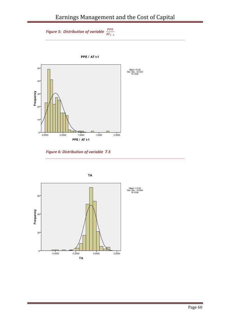
deviation in the skewness and kurtosis24 measures (Table 6-1). Furthermore data is plotted and an

informed decision is adopted (Appendix Figure 3-6)(Field, 2005, p. 93). Outliers based on z–scores

total

Table 6-1: Descriptive Statistics for the variables 𝟏𝑨𝑻𝒕−𝟏

, 𝜟𝑹𝑬𝑽𝑨𝑻𝒕−𝟏

, 𝑷𝑷𝑬𝑨𝑻𝒕−𝟏

& 𝑇𝐴

23

The Kolmotorov-Smirnov and Shapiro-Wilk tests are designed to measure whether data is normally distributed. However, they seem less significant when sample size is great (N>200). (Field, 2005, p. 93)

24 A distribution that is not normal is either not symmetric (skewness) or too pointy (kurtosis). Statistical tests can be performed to measure the degree of kurtosis or skewness. Values that deviate from 1 indicate a deviation from a normal distribution (Field, 2005, pp. 8-10).


Page 38

Table 6-2: Parameter values for the variables used in the Modified Jones

model(Dechow, Sloan, & Sweeney, Detecting earnings management, 1995)

In accordance with Bergstresser and Philippon (2006) and Francis et al. (2005, p. 303), 98%

Winsorizing will be applied to determine outliers. This entails that 2% of the data is considered an

outlier. All the data lower than the 1 percentile and above the 99 percentile will be transformed.

(Field, 2005, p. 78). Outliers are not deleted, as this would distort the data. Nevertheless, they are

transformed. Data that is greater than the 99 percentile is transformed to the highest value within

the 99 percentile. Data lower than the 1 percentile is transformed to the lowest value above the 1

percentile.

Industry Model B Std. Error β t

(Constant) α0 0.281 0.115 2.443 ***

1 / AT t-1 α1 -159.133 45.034 -1.140 -3.534 **

R2 = .583 ΔREV / AT t-1 α2 0.089 0.162 0.143 0.550

PPE / AT t-1 α3 -0.639 0.253 -0.921 -2.526 ***

(Constant) α0 -0.008 0.023 -0.326

1 / AT t-1 α1 85.527 134.718 0.136 0.635

R2 = .256 ΔREV / AT t-1 α2 0.033 0.015 0.677 2.133 ***

PPE / AT t-1 α3 -0.085 0.042 -0.630 -2.011

(Constant) α0 -0.013 0.013 -0.992

1 / AT t-1 α1 -7.952 6.374 -0.129 -1.248

R2 = .078 ΔREV / AT t-1 α2 -0.010 0.019 -0.054 -0.512

PPE / AT t-1 α3 -0.068 0.029 -0.244 -2.326 ***

(Constant) α0 -0.028 0.018 -1.518

1 / AT t-1 α1 34.285 22.662 0.234 1.513

R2 = .129 ΔREV / AT t-1 α2 0.023 0.035 0.113 0.671

PPE / AT t-1 α3 -0.098 0.056 -0.289 -1.749

(Constant) α0 -0.067 0.011 -6.298 *

1 / AT t-1 α1 34.467 10.943 0.587 3.150 **

R2 = .437 ΔREV / AT t-1 α2 -0.032 0.017 -0.309 -1.828

PPE / AT t-1 α3 -0.022 0.022 -0.176 -1.005

(Constant) α0 -0.879 0.198 -4.445 ***

1 / AT t-1 α1 -2575.217 8212.831 -0.294 -0.314

R2 = .887 ΔREV / AT t-1 α2 7.959 3.361 0.764 2.368

PPE / AT t-1 α3 2.403 1.343 1.717 1.789

(Constant) α0 -0.122 0.031 -3.878 *

1 / AT t-1 α1 3.254 5.363 0.093 0.607

R2 = .315 ΔREV / AT t-1 α2 0.207 0.056 0.591 3.692 *

PPE / AT t-1 α3 0.197 0.176 0.183 1.119

The significance of 0.001; 0,01 and 0,05 are respectively denoted by *; ** and ***

Unstandardized

Coefficients

Standardized

Coefficient

0001 - Oil & Gas

1000 - Basic Materials

6000 - Telecommunications

9000 - Technology

2000 - Industrials

3000 - Consumer Goods

5000 - Consumer Services


Page 39

The sample of firms has been categorized according to the ICB classification25. A model has been

created from the first stage of the Jones model (Jones, 1991), where the estimated accruals (𝐸 𝑇𝐴 )

are calculated. Table 6-2 presents the value (𝛽) for the industry relevant parameters that will be

used in the modified Jones model (Dechow, Sloan, & Sweeney, 1995). At this stage it must be noted

that slitting the sample into industry, reduces the reliability. Field (2005, p. 172) notes that the

stronger the correlation between predictor variables and the outcome variables, the bigger the

sample.

Table 6-3: Sample size per industry

Unfortunately there is no exact calculation that determines the sample size. Field (2005, pp. 172-

173)26 states that two common benchmarks are used, i.e. 10 or 15 cases per predictor variable.

Using the former, this would entail a sample size per industry of 30 cases (10×3). As seen in table 6-

3, four industries fail to meet the 30 cases needed for a reliable outcome. This should be noted as a

possible limitation to the results.

6.2 Descriptive statistics

Based on the previous paragraph’s outcome, the industry parameters are entered into equation 5-3.

This determines the |𝐷𝐴| variable, and completes the necessary variables for further study. In

coherence to the previous paragraph, outliers are detected and transformed by means of

Winsorizing. In table 6-3, an overview is provided of the variables used throughout this research. The

average cost of debt is 4.96%, and the average cost of equity is 6.11%.

25

ICB classification uses four levels of classification. For this research, only the first level will be used, due to sample size. Dividing companies into further sub-sections would reduce the sample size per section.

26 According to Field, there is no real calculation in determining sample size. Among the two measures used in this research, Field notes a number of other calculations that can be made. However this “oversimplifies the problem”, leaving the determination of the sample size up to the researcher. (Field, 2005, pp. 172-174)

Industry Firm years

0001 - Oil & Gas 14

1000 - Basic Materials 21

2000 - Industrials 91

3000 - Consumer Goods 42

5000 - Consumer Services 27

6000 - Telecommunications 7

9000 - Technology 35

Total 237


Page 40

Table 6-4: Overview of variables.

The central equation in this research, equation 5-8 and equation 5-9 will be calculated. Prior to

calculating these equations, the effect of the predictor variables have on the outcome variable |𝐷𝐴|

and 𝑆𝑚𝑜𝑜𝑡𝑕𝑖𝑛𝑔 must be measured. Therefore, the control variables are initially ignored.

6.2.1 Results from an uncontrolled model

Discretionary model (|𝑫𝑨|)

Concluded from the model summary (Table 2, Appendix), 𝐶𝑜𝑠𝑡𝐷𝑒𝑏𝑡 and 𝐶𝑜𝑠𝑡𝐸𝑞𝑢𝑖𝑡𝑦 only account

for 1.6% of the change in |𝐷𝐴|.𝑅2 for model 𝐷𝐴 = 𝛽0 + 𝛽1 × 𝐶𝑜𝑠𝑡𝐷𝑒𝑏𝑡 + 𝛽2 × 𝐶𝑜𝑠𝑡𝐸𝑞𝑢𝑖𝑡𝑦 is

.016. The values of the parameters 𝛽0 ,𝛽1 ,𝛽2 are respectively .051, .109, .106 (Table 6-5).

Table 6-5: Coefficients for uncontrolled model

The information above concludes that, the predictor variables in themselves do not explain the

changes in outcome variable. Only 1.6% of the change in |𝐷𝐴| can be allocated to the predictor

variables 𝐶𝑜𝑠𝑡𝐷𝑒𝑏𝑡 and 𝐶𝑜𝑠𝑡𝐸𝑞𝑢𝑖𝑡𝑦. The F-ratio for the model without control variables is greater

than one (F change =3.622), indicating that the model does predict |𝐷𝐴| better than the mean.

Moreover, the F-change ratios is greater than .05 significant (p = .058), rendering the value as

unsuitable to model on |𝐷𝐴|.

Model B Std. Error β

(Constant) β0 0.051 0.010 *

CostDebt β1 -0.109 0.165 -0.043

CostEquity β2 -0.106 0.056 -0.125


R2 = .016

Standardized

Coefficient

Unstandardized

Coefficients


Page 41

Coefficients of the model also indicate that there is no strong relation between the predicator

variable and the outcome variable. 𝐶𝑜𝑠𝑡𝐷𝑒𝑏𝑡 and 𝐶𝑜𝑠𝑡𝐸𝑞𝑢𝑖𝑡𝑦 only influence |𝐷𝐴| by -.109 and -

.106, respectively. However, it must be said that the coefficients are not significant.

It is also worth noticing the direction of the coefficients used in the model (Table 6-4). Although the

predictors are not significant, the operator gives an indication of the relation between the predictor

variables and the outcome variables. The (-) indicates that the negative relation between the

variables. This would suggest that the greater the cost of debt or the greater the cost of equity, the

less earnings management would be suspected.

𝑺𝒎𝒐𝒐𝒕𝒉𝒊𝒏𝒈

In Table 3 (Appendix), an overview is given of a model using the smoothing proxy as an outcome

variable. The model has must less predictor power on 𝑆𝑚𝑜𝑜𝑡𝑕𝑖𝑛𝑔 than |𝐷𝐴|. 𝑅2 is .008, indicating

that the model explains 0.8% of the variation in 𝑆𝑚𝑜𝑜𝑡𝑕𝑖𝑛𝑔. The predictor variables are not a better

variable than the mean. The F-ratio is smaller than one, suggesting that the mean explains the

variation in 𝑆𝑚𝑜𝑜𝑡𝑕𝑖𝑛𝑔 better than the two predictor variables used in this model.

Table 6-6: Coefficients for uncontrolled model, with 𝑺𝒎𝒐𝒐𝒕𝒉𝒊𝒏𝒈 as outcome

Unlike the previous model, the influences of the two variables differ a great deal. 𝐶𝑜𝑠𝑡𝐷𝑒𝑏𝑡 and

𝐶𝑜𝑠𝑡𝐸𝑞𝑢𝑖𝑡𝑦 respectively have coefficients of 21.907 and-8.803. Although both 𝐶𝑜𝑠𝑡𝐷𝑒𝑏𝑡 and

𝐶𝑜𝑠𝑡𝐸𝑞𝑢𝑖𝑡𝑦 have a great influence on the model, the results are not significant. Moreover, they

influence a model that in itself fails to explain 𝑆𝑚𝑜𝑜𝑡𝑕𝑖𝑛𝑔

Besides the influence the models have on the regression, the direction of the predictor variables

differ. The variable direction of 𝐶𝑜𝑠𝑡𝐸𝑞𝑢𝑖𝑡𝑦 is unchanged compared to the previous model

(equation 5-8). However, 𝐶𝑜𝑠𝑡𝐷𝑒𝑏𝑡 has changed. The previous model indicated a negative

correlation between the predictor and outcome variable. When the outcome variable changed

to 𝑆𝑚𝑜𝑜𝑡𝑕𝑖𝑛𝑔, the correlation is positive.


(Constant) β0 2.554 1.582

CostDebt β1 21.907 27.459 0.052

CostEquity β2 -8.803 9.243 -0.063


R2 = .008

Standardized

Coefficient

Unstandardized

Coefficients


Page 42

6.2.2 Results from controlled model

Discretionary model (|𝑫𝑨|)

The results that were given from the uncontrolled model were not significant to conclude any

reasonable conclusion. The negative correlation between the predictor variables and the outcome

variables was as expected. In the next model all the controlled variable are added, except for

industry (equation 5-10). The reason for this is that, first a general impression will be given of the

model. Further in this research the model will be presented per industry and differences analyzed27.

Table 6-7: Model summary of model with control variables, |𝑫𝑨|

Table 6-7 gives an overview of the model as difference control variables are added. The model has

improved, compared to the model where no control variables were used. However, the

improvement is not radically enhanced. 𝑅2 has improved from .016 to .087. This suggests that the

model explains 8.7% of the change in |𝐷𝐴|. Although the model explains a small portion of the

changes in |𝐷𝐴|, the F-ratio shows a significant improvement to the mean (Sig. F-Change < .05). The

model models |𝐷𝐴| more than seven times better that the mean.

27

Another reason for excluding industry for the time being is the type of variable industry is. Whereas the control variable𝑠 𝐿𝑒𝑣𝑒𝑟𝑎𝑔𝑒, 𝑆𝑖𝑧𝑒, 𝑅𝑂𝐴, 𝐼𝑛𝑡𝑒𝑟𝑒𝑠𝑡𝐶𝑜𝑣𝑒𝑟𝑎𝑔𝑒 and 𝐺𝑟𝑜𝑤𝑡𝑕 are numeric ration measures, 𝐼𝑛𝑑𝑢𝑠𝑡𝑟𝑦 is a nominal measure. This implies that the latter level of measurement is used for categorizing information. The former level of measurement has structural characteristics, i.e. mathematical attributes. (Babbie, 2007, pp. 137-139)


Page 43

Table 6-8: Coefficients for model with control variables, |𝑫𝑨|

In accordance to the previous model (without control variables), the relation between the predictor

variable and the outcome variable is the same. However, the values have no significant impact on

the model. The only significant coefficients are the control variables 𝑅𝑂𝐴 and 𝐺𝑟𝑜𝑤𝑡𝑕.

Notable is table 6-8 is the direction of the coefficient 𝐵. In accordance to the model with no control

variables, the variables 𝐶𝑜𝑠𝑡𝐷𝑒𝑏𝑡 and 𝐶𝑜𝑠𝑡𝐸𝑞𝑢𝑖𝑡𝑦 are both negatively correlated to |𝐷𝐴|.

Furthermore the control variables 𝐿𝑒𝑣𝑒𝑟𝑎𝑔𝑒 and 𝑅𝑂𝐴 are also negatively correlated.

Smoothing

Table 6-9: Model summary of model with control variables, 𝑺𝒎𝒐𝒐𝒕𝒉𝒊𝒏𝒈

The model considerably improves once the control variables have been added to the equation. The

model improved to explain 3% of the variation in 𝑆𝑚𝑜𝑜𝑡𝑕𝑖𝑛𝑔. However, the improvement of the

model is derived from the significance of the model (𝑝 < .05). The previous model predicted next to


(Constant) 0.066 0.019 *

CostDebt -0.079 0.169 -0.031

CostEquity -0.075 0.060 -0.088

Leverage -0.037 0.020 -0.124

Size 0.001 0.004 0.016

ROA -0.164 0.054 -0.207 **

InterestCoverage 0.001 0.001 0.072

Growth 0.021 0.008 0.175 **


R2 = .087

Unstandardized

Coefficients

Standardized

Coefficient


Page 44

nothing and was not significant. A model with control variables shows a significant influence on the

outcome variable. Furthermore, the model is a better fit to 𝑆𝑚𝑜𝑜𝑡𝑕𝑖𝑛𝑔 than the mean.

In accordance to the uncontrolled model, the difference between the variables 𝐶𝑜𝑠𝑡𝐷𝑒𝑏𝑡 and

𝐶𝑜𝑠𝑡𝐸𝑞𝑢𝑖𝑡𝑦 remain relatively high. 𝐶𝑜𝑠𝑡𝐷𝑒𝑏𝑡 has a relatively large influence on the outcome

variable 𝑆𝑚𝑜𝑜𝑡𝑕𝑖𝑛𝑔. Apparent is that in contradiction to the previous models, 𝐶𝑜𝑠𝑡𝐷𝑒𝑏𝑡 has a

positive effect on the outcome. Prior models show a negative correlation between the outcome

variable and the two predictors.

Table 6-10: Coefficients for model with control variables, 𝑺𝒎𝒐𝒐𝒕𝒉𝒊𝒏𝒈

6.2.3 Industrial influence

Discretionary model |𝑫𝑨|

The outcome for the industry control variable is presented in Table 3 of the Appendix. In all

industries, 𝑅2 has improved, exceeding .087. Though, it does not result in a significant improvement

for all industries. Only two industries profit from a significant result, i.e. 2000 and 3000. However

looking at table 6-11, it is notable that the value for industry 6000 – Telecommunications, i.e. 𝑅2 =

1. This would entail a perfect correlation (multicollinearity )28 between the model and |𝐷𝐴|,

generating an undesirable effect (Field, 2005, p. 174). An explanation for the high residual variant is

the small sample used in this industry sample (Table6-3), rendering the value as not significant.

Examining table 6-8 further, 𝑅2 differs between the industries, generally improving the model

stated in equation 5-8. However, the model is not always a better fit than the mean. Suggesting that

28

Multicollinearity occurs when there is a strong correlation between predictor variables and outcome variable. This occurrence poses a number of threats to a regression analysis: (1) limits 𝑅2, (2) difficult to determine the measure of important of independent variables and (3) creates unstable variables. (Field, 2005, p. 174)


(Constant) 0.783 3.312

CostDebt 28.004 28.752 0.067

CostEquity -8.046 10.194 -0.057

Leverage 0.763 3.471 0.016

Size 0.452 0.762 0.043

ROA 1.150 9.266 0.009

InterestCoverage -0.073 0.198 -0.026

Growth -2.729 1.306 -0.141 ***


R2 = .030

Unstandardized

Coefficients

Standardized

Coefficient


Page 45

deviation from the average |𝐷𝐴| could be a better signal for the use earnings management. Only

industries 1000, 2000 and 3000 produce an improved model, however is must be noted that only in

industry 2000 – Industrials is this improvement significant.

Table 6-11: 𝑹𝟐 F-ratio and Mean per industry, |𝑫𝑨|

It is worth noticing the direction of the two predictor variables. In a model were no concern was

taken for the different industries, a negative correlation was found between the predictors and the

outcome. However, when controlling for industries, not one industry finds both predictors

negatively correlated to the outcome. Industries 0001 and 3000 perceive 𝐶𝑜𝑠𝑡𝐷𝑒𝑏𝑡 as positively

related to |𝐷𝐴|. Industry 9000, considers 𝐶𝑜𝑠𝑡𝐸𝑞𝑢𝑖𝑡𝑦 as positively correlated. The remaining three

industries 1000; 2000 and 5000, regard both 𝐶𝑜𝑠𝑡𝐷𝑒𝑏𝑡 and 𝐶𝑜𝑠𝑡𝐸𝑞𝑢𝑖𝑡𝑦 as positively correlated to

|𝐷𝐴|. The influence on the model differs per industry (Table 4, Appendix). However, in general the

mean 𝐶𝑜𝑠𝑡𝐸𝑞𝑢𝑖𝑡𝑦 is higher than the mean 𝐶𝑜𝑠𝑡𝐷𝑒𝑏𝑡 (Table 6-11).


Consistent with the previous model, adding 𝐼𝑛𝑑𝑢𝑠𝑡𝑟𝑦 as control variable improves the predictive

power of most industries. However none of the industries report significant results. Table 5

(Appendix) gives a good overview of the results per industry. A remarkable result is the change in the

F-ratio. Before the model was controlled by industry, the F-ratio was 4.367. This indicates that the

model was a better fit than the mean. Once Industry was introduced as control variable, this ratio

has declined in all industries. In table 6-12 it is apparent that three of the six valid values is below

one.

Consistent with the previous model with the outcome variable of |𝐷𝐴|, the industry 6000 returns

invalid results. Further research into the reason for the void results, predicts limitations with the

sample. Adapted models have been applied to the current sample, but return non significant results.

CostDebt CostEquity

0001 - Oil & Gas .628 .129 .731 .044 .081

1000 - Basic Materials .515 4.015 .066 .038 .075

2000 - Industrials .197 16.152 .000 .049 .058

3000 - Consumer Goods .433 4.935 .033 .049 .056

5000 - Consumer Services .323 .153 .700 .050 .041

6000 - Telecommunications 1.000 N/A N/A .050 .098

9000 - Technology .254 .761 .391 .051 .053

Industry Sig. F ChangeF ChangeR 2 Mean


Page 46

Table 6-12: 𝑹𝟐 F-ratio and Mean per industry, 𝑺𝒎𝒐𝒐𝒕𝒉𝒊𝒏𝒈

6.3 Results accrual approach

In this paragraph, the result will be presented that were achieved through statistical analysis. First

the preliminary results will be presented. Consequently, some insight will be provided into whether

the results hold for the population and can be generalized. Based on the outcome of the

generalization, the final results for the model are noted.

6.3.1 Preliminary results

The models containing only the predictor and outcome variables do not provide a good explanation

for |𝐷𝐴| or 𝑆𝑚𝑜𝑜𝑡𝑕𝑖𝑛𝑔. The cost of debt and the cost of equity seem to have better predicting

power over |𝐷𝐴| than 𝑆𝑚𝑜𝑜𝑡𝑕𝑖𝑛𝑔. However, none of these models seem significant. The first model

was only able to support 1.6% of the variation in 𝐷𝐴 , i.e. accrual based earnings management.

Although the model was does not explain |𝐷𝐴| that well, it seems to be a better fit of a model than

the mean. The second model was only able predict 0.08% of the outcome, 𝑆𝑚𝑜𝑜𝑡𝑕𝑖𝑛𝑔. However,

the F-ratio29 was below zero ensuring that the model was not a better fit than the mean.

𝐶𝑜𝑠𝑡𝐷𝑒𝑏𝑡 has the most influence on the model relating to 𝑆𝑚𝑜𝑜𝑡𝑕𝑖𝑛𝑔, compared with 𝐶𝑜𝑠𝑡𝐸𝑞𝑢𝑖𝑡𝑦.

However, in contradiction to the |𝐷𝐴| model, 𝐶𝑜𝑠𝑡𝐷𝑒𝑏𝑡 is positively correlated to 𝑆𝑚𝑜𝑜𝑡𝑕𝑖𝑛𝑔.

Unlike the 𝑆𝑚𝑜𝑜𝑡𝑕𝑖𝑛𝑔 model, the cost of debt and the cost of equity have an equal influence on

|𝐷𝐴|. Despite all these results, both models reveal no significant answers.

Controlled Model

An improvement was noted when the initial five control variables were introduced. The controlled

model was able to predict the outcome variable better. In the model with the outcome variable

|DA|, the explanatory power improved to 8.7%. Furthermore, the F-ratio increased to over seven.

More specifically, this model explains |DA| seven times better than the mean. An uncontrolled

29

The F-ratio measures improved outcome of the model compared to the inaccuracy. A value greater than 1 suggests an improved outcome greater than the inaccuracy. (Field, 2005, p. 150)

CostDebt CostEquity

0001 - Oil & Gas .786 1.023 .351 .044 .081

1000 - Basic Materials .283 .828 .379 .038 .075

2000 - Industrials .048 2.449 .121 .049 .058

3000 - Consumer Goods .231 1.840 .184 .049 .056

5000 - Consumer Services .401 .333 .570 .050 .041

6000 - Telecommunications 1.000 N/A N/A .050 .098

9000 - Technology .084 .139 .712 .051 .053

Industry Sig. F ChangeF ChangeR 2 Mean


Page 47

model only 3.6 times the mean. Moreover, the predictability powers of the model are significant.

(𝑝 = .008 < .05).

An improvement on the model with the outcome variable 𝑆𝑚𝑜𝑜𝑡𝑕𝑖𝑛𝑔 was also noted. The

explanatory power was not as great as in other model (outcome variable = |𝐷𝐴|). However

compared to the uncontrolled model, the predictability powers increase to 3%. Furthermore, the

model became a better fit (F-ratio = 4.367). The results about this model are also significant

(𝑝 = .038 < .05). It should be noted though that, the coefficient for 𝐶𝑜𝑠𝑡𝐷𝑒𝑏𝑡 increased, and

remained positive. Although an increase would suggest a better model for the predictor variables,

𝐶𝑜𝑠𝑡𝐸𝑞𝑢𝑖𝑡𝑦 remained relatively unchanged.

Industry influence

The control variable 𝐼𝑛𝑑𝑢𝑠𝑡𝑦 allows the model to be view per industry. As stated above, different

industries have different instruments and incentives to apply the use of earnings management. From

the statistical research, it is evident that different industries are affected by different variables.

Furthermore, it is evident that industries react differently to different models. Although not all

variables are significant, there are vast differences in how the control variables affect the outcome.

Using industries to control our model, has drastically improved the explanatory power of the model.

Table 4 and Table 5 (Appendix) provide an overview of 𝑅2 per industry. Nevertheless, the increase in

𝑅2 is not significant. The influence of the proxy 𝐶𝑜𝑠𝑡𝐷𝑒𝑏𝑡 and 𝐶𝑜𝑠𝑡𝐸𝑞𝑢𝑖𝑡𝑦 seem to vary over the

industries. The direction of the variables differ enormously though the different industries. Not

controlling for 𝐼𝑛𝑑𝑢𝑠𝑡𝑟𝑦, 𝐶𝑜𝑠𝑡𝐷𝑒𝑏𝑡 and 𝐶𝑜𝑠𝑡𝐸𝑞𝑢𝑖𝑡𝑦 were both negatively correlated to |𝐷𝐴|.

However with the introduction of industries, not one industry had the same correlation direction as

the uncontrolled model. With regards to 𝑆𝑚𝑜𝑜𝑡𝑕𝑖𝑛𝑔, only three of the six industries portrayed the

same correlation.

6.3.2 Generalization

It is important that the results acquired from our sample are relevant to the whole population. This

ensures that the statements made based on the sample used, can be valid for the population. When

performing a statistical test, certain assumptions are made. Field (2005, pp. 169-175) explains a

number of aspects that should be addressed to improve the quality of the results. This sub-

paragraph will address these relevant issues that will address these assumptions.

Cross-validation

In assessing the cross-validation, the value of the adjusted 𝑅2 will be considered. The adjusted 𝑅2

indicates whether 𝑅2 will change if the results were valid to the population. Therefore the adjusted

𝑅2 indicates a modification in the predictive power or the shrinkage in the population (Field, 2005,


Page 48

p. 171)30. The uncontrolled model was neither highly explanatory of our outcome, nor significant and

will not be considered. Our first model with control variables presents a very small predictive power,

indicating that the model had low predicting power in the sample. However, when modeling the

|𝐷𝐴| variable, the adjusted 𝑅2 decreased. The value of the adjusted 𝑅2 is .059, indicating that a

predictability factor of 5.9% on the population. Although this value is still significant, the adjusted 𝑅2

decreases by 32% compared to the original 𝑅2.

With regards to 𝑆𝑚𝑜𝑜𝑡𝑕𝑖𝑛𝑔, the model has a significant 𝑅2 value. However, the adjusted value

descends to .000, losing all predictability in the population.

When industry is introduced as control variable, the adjusted 𝑅2 was generally lower than 𝑅2.

Nevertheless, none of the industry models significantly predict the outcome variable. As the models

cannot predict the sample significantly, a robustness test on the fit in the population seems

insignificant.

Multicollinearity

It is important that the variables used to explain the outcome variable do not have a perfect

correlation. However in industry 6000 – Telecommunications, 𝑅2 is 1. This would suggest that the

model perfectly correlates to |𝐷𝐴| and 𝑆𝑚𝑜𝑜𝑡𝑕𝑖𝑛𝑔. It might sound appeasing to know that the

perfect model is found to predict the outcome, however is comes with some statistical short fall.

Although the model might suit the sample well, it limits any conclusion about effects on the

population. Furthermore, high collinearity limits the explanatory value 𝑅2 and increases the

standard error (Field, 2005, p. 174). According to Field there is not much that can be done about a

perfect correlation. However, increasing the size of the sample in this industry could help the

problem.

6.4 Hypotheses results and Summary

In chapter four, four hypotheses were presented. These hypotheses will be reevaluated, based on

the empirical evidence presented in above. This presents a summary for the chapter

Discretionary accruals

A model with no control variables does little to predict the use of earnings management. Within the

boundaries of the discretionary accrual model, the cost of equity does not prove to have a great

influence on the outcome. The effects of cost of equity and the cost of debt are not significant for

detecting the use of earnings management by itself. Based on the initial statistical research, H-01 and

H-02 cannot be rejected.

30

When assessing the adjusted 𝑅2, the difference between the original 𝑅2 and the adjusted value must be evaluated.


Page 49

A better view is presented using control variables. However the predictor power of these models

decreased when controlled for industries. With regards to the discretionary accruals, the effects of

the cost of equity are relatively similar to those of the cost of debt. Therefore, the influence on the

cost of equity and the cost of debt are comparable. Although the variables could only predict a small

relation, it is was highly significant (p=.038). The association between the cost of debt and the

discretionary accruals did decline when controlling for other aspects. Performance measures have a

greater association with discretionary accruals. As expected the cost of equity is negatively

correlated with discretionary accruals. Based on the above, it is possible to reject the H-01 and H-02,

and accept H1 and H2. Therefore, once controlled for leverage; size; ROA; interest coverage and

growth, the cost of equity and the cost of debt are negatively correlated to the discretionary

accruals.

Smoothing

With regards to smoothing, a relatively smaller correlation was noted. Although the 3% correlation is

smaller than on discretionary accruals, it is found significant. Unlike the discretionary accrual model,

the cost of equity has less common properties with the cost of debt. The cost of debt is noted to be

positively correlated, compared to the negative correlation observed by the cost of equity.

Furthermore, the cost of debt has a far greater influence on smoothing than the cost of equity. The

coefficients for the cost of debt are 28.004 compared to the -8.046 coefficient by the cost of equity.

A disadvantage of the discretionary accrual model is the drop in coefficient values once control

variables are added. The smoothing models either increase their coefficients or remain the same.

This indicates the strength of the variables. Based upon the above the H-02 and H-04 can be rejected.

Once controlled for leverage; size; ROA; interest coverage and growth, the cost of equity is

negatively correlated to smoothed earnings and the cost of debt positively correlated to smoothed

earnings.

The next chapter will present the conclusion for this research. The main research question will be

answered. Furthermore, limitations to the research will be presented, with suggestions for further

research.


Page 50

7 Conclusion

In the previous chapter the results related to the hypotheses were noted. In this chapter, the main

research question that was stated in the first chapter will be answered. Throughout this paper,

different aspects of the research question have been addressed. Firstly, a literature study was done

to support a framework for in which further study was made possible. Within the literature research

two main subjects were addressed i.e. the use of earnings management and the cost of capital. In

general the cost of capital addressed as one category; thereafter two separate forms were

distinguished. Based on the literature framework, four hypotheses were developed. These were

followed by the research design and the empirical research. In contrast to prior research, this

research focused on Dutch stock listed companies.

In addition to answering the main research question, limitation that this research faced will be noted

and explained. During this study the focus was on explaining incentives for the use of earnings

management. For this reason, the outcome (dependant) variable was the use of earnings

management, with proxies 𝐷𝐴 and 𝑆𝑚𝑜𝑜𝑡𝑕𝑖𝑛𝑔. Previous studies conducted by Francis et al.

(2005); Francis et al. (2008); and Prevost et al.(2008) are related to the subject that concerns this

paper.

7.1 Conclusions and Limitations

7.1.1 Earnings management and the cost of equity

Francis et al. (2005) suggests that investors are aware of the management’s incentive to manage

earnings through accruals. However, Francis et al. (2005) only associated inflated discretionary

accruals with a greater equity beta. This insinuates that high beta’s are associated with high returns.

According to financial theory, this relation is apparent.

In this research no evidence was found to substantiate that the cost of capital was not associated

with earnings management (null-hypothesis). Only in a controlled environment was a connection

found between the cost of capital and earnings management. A strong factor in the research of

Francis et al. (2005) is the sample size used to investigate earnings management. Francis et al. (2005)

took a sample of US firms between 1970 and 2001, totaling 76,195 firm years. This highlights one of

the reasons this study fail to make any significant statement about the relation between earnings

management and the cost of equity. Although in a controlled environment a significant relation was

found, the model was only able to capture 8.7% of discretional earnings management and 3% of

smoothed income. Firms that are controlled by industry codes seem to loss their predictability for

the use of earnings management. The relation is greater; however the results are not significant.

Gray et al. (2009) performed a similar study with Australian firms. A conclusion that derived from

that study was that the cost of equity is not necessarily driven by the discretionary component of the


Page 51

accrual. Gray et al. states that due to constitutional differences, Australian firms are more likely to

associate the cost of capital to the innate element of the accruals.

7.1.2 Earnings management and the cost of debt

An extensive study on the cost of debt was performed by Prevost et al. (2008). They concluded that

investors see though the intentions of optimistic managers. Prevost et al. further states that, there is

evidence to support the notion that earnings management increases the cost of debt. Although this

is measure using marginal debt obtained in the bonds market, these conclusions are supported by

other researches (Francis, LaFond, Olsson, & Schipper, 2005).

This study however presents a less apparent view on the issue. Investors seem to be unaware of

earnings management through discretionary accruals. Greater accruals result in lower return rates

on debt. If investors were aware of the possibilities of inflated earnings, they would incorporate this

in their expected return. However, there is a great difference on the form of earnings management.

Accrual inflation is indeed associated with a lower cost of debt. On the other hand, smoothing is

positively associated with high cost of capital. Therefore, investors are aware of a firm’s intention to

smoothing earnings over time. A rational reason would be that detecting smoothed earnings is less

complicated. There are numerous ways in which discretional accruals can be measured. It must be

stated though, that these conclusion are only valid in a controlled environment.

The relation between the cost of capital and earnings management is significant. However as stated

in chapter 2, there are numerous incentive for managers to manage earnings. The cost of capital is

one of these, however not the most important. Studies carried out prove that a much stronger

relation can be found between earnings management and incentive packages offered to mangers.

Nonetheless, investors should be aware of intentions of firms. The influence between the cost of

equity (dividend payout) and the cost of debt (interest expenses) differs. In general, equity has a

lower influence on the earnings management proxies. This could be a result of the initiators of the

dividend payout. Returns from debt are contractually fixed and agreed upon. Formally the dividend

payout is determined by the equity holders, however in reality the firm decides the amount it is

willing to pay.

7.2 Further research

The majority of researches performed on earnings management are held in the US. Gray et al.

(2009)performed a study in Australia, highlighting the institutional differences between the two

countries. Although this study demonstrates the situation in the Netherlands, institutional difference

could be thought for further studies.


Page 52

A great limitation of this study is the limited sample size. Francis et al. (2005)used a sample of 76,195

firm years, spread over 30 years. This sample size might be too ambitious for the Netherlands;

however a greater sample over time would improve the results. This accompanied by a greater

understanding of the institutional settings, could shed more light in the incentives firms have to

manage earnings.


Page 53

Bibliography

Aharony, J., & Swary, I. (1980). Quarterly Dividend and Earnings Announcements and Stockholders' Returns:

An Empirical Analysis. The Journal of Finance , 35 (1), 1-12.

Babbie, E. (2007). The practise of social research (11th ed.). Belmont: Thomson Wadsworth.

Bauman, M. P., & Shaw, K. W. (2006). Stock option compensation and the likelihood of meeting analysts’

quarterly earnings targets. Review of quantitative finance and Accounting , 26, 301-319.

Beneish, M. D. (2001). Earnings Management: A Perspective. Managerial Finance , 27 (12), 3-17.

Beneish, M. D. (1999). Incentives and Penalties Related to Earnings Overstatements That Violate GAAP. The

Accounting Review , 74 (4), 425-457.

Bergstresser, D., & Philippon, T. (2006). CEO incentives and earnings management. Journal of Financial

Economics , 511-529.

Bradley, M., & Roberts, M. (2004). The structure and pricing of corporate debt covenants. Working Paper, Duke

University.

Brav, A., Harvey, C. R., & Michaely, R. (2005). Payout policy in the 21st century. Journal of Financial Economics ,

77 (3), 483-527.

Brealey, R. A., Myers, S. C., & Allen, F. (2006). Corporate Finance (8th ed.). Ney York: McGraw-Hill Irwin.

Cheng, Q., & Warfield, T. (2005). Equity incentives and earnings management. Accounting Review , 80, 441–

476.

Coles, J. L., Hertzel, M., & Kalpathy, S. (2006). Earnings management around employee stock option reissues.

Journal of Accounting and Economics , 41 (1-2), 173-200.

Daniel, N. D., Denis, D. J., & Narveen, L. (2008). Do firms manage earnings to meet dividend thresholds?

Journal for Accounting and Economics , 45, 2-26.

DeAngelo, H., & DeAngelo, L. (2006a). The irrelevance of the MM dividend irrelevance theorem. Journal of

Financial Economics , 79 (2), 293-315.

DeAngelo, L. E. (1986). Accounting Numbers as Market Valuation Substitutes: A Study of Management Buyouts

of Public Stockholders. The Accounting Review , 61 (3), 400-420.

Dechow, P. M., & Sloan, R. G. (1991). Executive incentives and the horizon problem: An empirical investigation.

Journal of Accounting and Economics , 14, 51-89.

Dechow, P. M., Sloan, R. G., & Sweeney, A. P. (1995). Detecting earnings management. The Accounting Review

, 70, 193-225.

Deschow, P. M., & Skinner, D. J. (2000). Earnings management reconciling the views of accounting academics,

practitioners and regulators. Accounting Horizons , 14 (2), 235-250.

Diamond, D., & Verrecchia, R. (1991). Disclosure, Liquidity, and the Cost of Capital. Journal of Finance , 46

(September), 1325-1359.

Easley, D., & O'Hara, M. (2004). Information and the Cost of Capital. The Journal of Finance , 59 (4), 1553-1583.

Field, A. (2005). Discovering Statistics Using SPSS. London: SAGE Publications Ltd. .

Francis, J., LaFond, R., Olsson, P., & Schipper, K. (2005). The pricing of accruals. Journal of Accounting

Economics , 39, 295-327.


Page 54

Francis, J., Nanda, D., & Olsson, P. (2008). Volentary disclosure, earning quality and cost of capital. Journal of

Accounting Research , 46 (1), 53-99.

Gao, P., & Shrieves, R. (2002). Earnings Management and Executive Compensation: A Case of Overdose of

Option and Underdose of Salary? Working Paper, University of Tennessee, Knoxville.

Gietzmann, M., & Ireland, J. (2005). Cost of Capital, Strategic Disclousure and Accounting Choice. Journal of

Business Finance & Accounting , 32 (April/May), 599-634.

Graham, J. R., Harvey, C. R., & Rajgopal, S. (2005). The economic implications of corporate financial reporting.

Journal of Accounting and Economics , 40, 3-73.

Gray, P., Koh, P., & Tong, Y. H. (2009). Accruals Quality, Information Risk and Cost of Capital: Evidence from

Australia. Journal of Business Finance & Accounting , 36 (1 & 2), 51-79.

Grullon, G., Michaely, R., & Swaminathan, B. (2002). Are Dividend Changes a Sign of Firm Maturity? The Journal

of Business , 75 (3), 387–424.

Healy, P. M. (1985). The effect of bonus schemes on accounting decisions. Journal of Accounting and

Economics , 7 (1-3), 85-107.

Healy, P. M., & Wahlen, J. M. (1999). A Review of the earnings management literature. Accounting Horizons ,

13 (4), 355-.

Hopkins, W. G. (2000, May 4). Quantitive research design. Retrieved Aug 4, 2009, from Sportscience:

http://www.sportsci.org/jour/0001/wghdesign.html

Jones, J. J. (1991). Earnings Management During Import Relief Investigations. Journal for Accounting Research ,

29 (1-2), 193-228.

Kim, O., & Verrecchia, R. E. (1995). Market liquidity and volume around earnings announcements. Journal of

Accounting and Economics , 17, 41–67.

Levitt, A. (2000, April 6). SEC Speech: Remarks at the Economic Club in Washington. Retrieved June 17, 2009,

from U.S. Security and Exchange Commission: http://www.sec.gov/news/speech/spch362.htm

Levy, H., & Post, T. (2004). Investments. Prentice Hall.

National Association of Certified Fraud Examiners. (1993). Cooking the books: What every accountant should

know about fraud. New York: NASBA.

Palepu, K. G., Healy, P. M., Bernard, V. L., & Peek, E. (2007). Business Analysis and Valuation, IFRS edition.

London: Cengage Learning EMEA.

Pettit, R. R. (1972). Dividend Announcements, Security Performance, and Capital Market Efficiency. The Journal

of Finance , 27 (5), 993–1007.

Prevost, A. K., Skousen, C. J., & Rao, R. P. (2008). Earnings Management and the Cost of Debt. Working paper,

Ohio State University, Department of Finance, Stillwater.

Rangan, S. (1998). Earnings arround seaconed equity offerings: Are they overstated? Journal of Financial

Economics , 50 (October), 101-122.

Ronen, J., & Yaari, V. (2008). Earnings Management; Emerging Insights in Theory, Practice, and Research. (First,

Ed.) New York: Springer.

Ronen, J., Tzur, J., & Yaari, V. L. (2006). The effect of directors’ equity incentives on earnings management.

Journal of Accounting and Public Policy , 25, 359-389.


Page 55

Roychowdhury, S. (2006). Earnings management through real activities manipulation. Journal of Accounting

and Economics , 42 (3), 335-370.

Skinner, D. J. (1993). The investment opportunity set and accounting procedure choice. Journal of Accounting

and Economics , 16 (4), 407-445.

Stein, J. C. (1989). Efficient Capital Markets, Inefficient Firms: A Model of Myopic Corporate Behavior. The

Quarterly Journal of Economics , 104 (4), 655-669.

Stolowy, H., & Breton, G. (2004). Accounts Manipulation: A Literature review and Proposed Conceptual

Framework. Review of Accounting & Finance , 3 (1), 5-66.

Teoh, S. H., & Wong, T. J. (2002). Why new issues and high accrual firms underperform: The role of analysts'

credulity. The Review of Financial Studies , 15 (3), 869–900.

Teoh, S. H., Welch, I., & Wong, T. J. (1998a). Earnings management and the long-run market performance of

initial public offerings. Journal of Finance , 53 (December), 1935-1974.

Teoh, S. H., Welch, I., & Wong, T. J. (1998b). Earnings management and the underperformance of seasoned

equity offerings. Journal of Finance , 50, 63-99.

Teoh, S. H., Wong, T. J., & Rao, G. R. (1998). Are Accruals during Initial Public Offerings Opportunistic? Review

of Accounting Studies , 3 (March), 175-208.

van Winsen, K. (2008). Executive compensation and earnings management. Working Paper, Erasmus University

Rotterdam, Rotterdam.

Vander Bauwhede, H. (2003). Resultaatsturing en kapitaalmarkten. Maandblad voor Accountancy en

Bedrijfseconomie , mei, 196-204.

Wald, J. (1999). Capital structure with dividend restrictions. Journal of Corporate Finance , 5, 193-208.

Watts, R. L., & Zimmerman, J. L. (1978). Positive accounting Theory of the determination of accounting

standards. The Accounting Review , 56 (January), 112-134.


Page 56

Appendix

Figure 1: Principles of Accounts Manipulation (Stolowy & Breton, 2004)


Page 57

Table 1: Survey responses to the question: Do the following factors contribute

to your company preferring a smooth earnings path? (Graham, Harvey, &

Rajgopal, 2005, p. 45)

Agree or

strongly

agree (%)

1 is perceived as less risky by investors 88.70

2 Makes it easier for analysts/investors to predict future 79.70

3 Assures customers/suppliers that business is stable 66.20

4 Reduces the return that investors demand (i.e. smaller risk premium) 57.10

5 Promotes a reputation for transparent and accurate 46.50

6 Conveys higher future growth prospects 46.30

7 Achieves or preserves a desired credit rating 42.20

8 Clarifies true economic performance 24.30

9 Increases bonus payments 15.60

Question: A smooth earnings path is preferred because it…


Page 58

Figure 2: Responses to the question: ‘‘Rank the three most important

measures report to outsiders’’ (Graham, Harvey, & Rajgopal, 2005, p. 20)


Page 59

Figure 3: Distribution of variable 𝟏

𝑨𝑻𝒕−𝟏

Figure 4: Distribution of variable 𝜟𝑹𝑬𝑽

𝑨𝑻𝒕−𝟏


Page 60

Figure 5: Distribution of variable 𝑷𝑷𝑬

𝑨𝑻𝒕−𝟏

Figure 6: Distribution of variable 𝑻𝑨


Page 61

Table 2: Model summary without control variables, outcome variable |𝑫𝑨|

Table 3: Model summary without control variables, outcome variable



Page 62

Table 4: Coefficients with industry as control variable, |𝑫𝑨|

Industry Model B Std. Error β

(Constant) 0.408 0.576

CostDebt 6.225 3.463 1.202

R2 = .628 CostEquity -0.570 1.023 -0.387

Leverage -0.714 0.665 -1.142

Size -0.006 0.073 -0.114

ROA -2.075 1.142 -1.086


Growth -0.023 0.065 -0.161

(Constant) -0.040 0.054

CostDebt 0.287 0.465 0.169

R2 = .515 CostEquity 0.079 0.123 0.330

Leverage 0.000 0.026 -0.003

Size 0.013 0.013 0.282

ROA -0.161 0.177 -0.494


Growth 0.015 0.008 0.594

(Constant) 0.049 0.037

CostDebt 0.085 0.228 0.041

R2 = .197 CostEquity 0.014 0.106 0.014

Leverage -0.028 0.032 -0.092

Size 0.000 0.011 0.004

ROA -0.174 0.098 -0.179


Growth 0.052 0.013 0.410 *

(Constant) 0.013 0.054

CostDebt 0.036 0.443 0.013

R2 = .433 CostEquity -0.146 0.090 -0.272

Leverage -0.032 0.047 -0.132

Size 0.010 0.012 0.211

ROA -0.090 0.141 -0.121


Growth -0.043 0.019 -0.320 ***

(Constant) -0.012 0.121

CostDebt 0.105 0.788 0.037

R2 = .323 CostEquity 0.433 0.401 0.411

Leverage -0.156 0.138 -0.559

Size 0.036 0.038 0.557

ROA -0.757 0.449 -0.679


Growth 0.008 0.022 0.083

(Constant) -0.083 0.125

CostDebt -0.294 0.594 -0.112

R2 = .254 CostEquity 0.346 0.401 0.273

Leverage -0.369 0.146 -0.753 ***

Size 0.089 0.042 0.598 ***

ROA -0.213 0.142 -0.294


Growth -0.029 0.033 -0.174



9000 - Technology

Unstandardized

Coefficients

Standardized

Coefficient

0001 - Oil & Gas


2000 - Industrials



Page 63

Table 5: Coefficients with industry as control variable, 𝑺𝒎𝒐𝒐𝒕𝒉𝒊𝒏𝒈

Industry Model B Std. Error β

(Constant) 31.834 17.800

CostDebt -217.176 107.042 -1.028

R2 = .786 CostEquity 13.025 31.626 0.217

Leverage -35.190 20.539 -1.380

Size -2.889 2.248 -1.287

ROA -23.383 35.290 -0.300


Growth -2.037 2.013 -0.344

(Constant) -19.665 38.632

CostDebt 633.461 332.617 0.634

R2 = .283 CostEquity -19.993 88.179 -0.141

Leverage -21.481 18.912 -0.402

Size 0.626 9.084 0.023

ROA 52.126 126.437 0.272


Growth -5.000 5.495 -0.328

(Constant) 2.085 8.362

CostDebt -12.940 51.004 -0.031

R2 = .048 CostEquity -29.051 23.735 -0.144

Leverage -0.342 7.181 -0.006

Size 0.978 2.502 0.047

ROA 13.642 21.834 0.068


Growth -4.513 2.884 -0.174

(Constant) -3.802 12.559

CostDebt 188.199 103.298 0.349

R2 = .231 CostEquity -13.749 21.083 -0.128

Leverage -3.598 11.013 -0.074

Size 0.508 2.710 0.051

ROA -28.112 32.812 -0.189


Growth -6.052 4.461 -0.228

(Constant) -9.531 10.994

CostDebt -46.630 71.347 -0.172

R2 = .401 CostEquity 16.233 36.284 0.160

Leverage 14.676 12.509 0.547

Size 1.057 3.408 0.169

ROA 60.923 40.625 0.568


Growth -1.126 1.951 -0.115

(Constant) 9.865 16.644

CostDebt 43.436 79.315 0.137

R2 = .084 CostEquity -64.206 53.552 -0.420

Leverage 8.597 19.461 0.145

Size -2.942 5.556 -0.165

ROA 3.021 19.029 0.035


Growth -1.659 4.454 -0.082



9000 - Technology

Unstandardized

Coefficients

Standardized

Coefficient

0001 - Oil & Gas


2000 - Industrials



Page 64

Author(s) Year Title paper Journal Object of study

Sample (sample size, country,

research period)

Methodology Results

#1 Beneish M.D.

2001 Earnings Management: A perspective

Managerial Finance

Provide a prospective on earnings management.

Not applicable - literature review



#2 Lang M., J.S. Raedy, W. Wilson

2006 Earnings management and cross listing: Are reconciled earnings comparable to US earnings?

Journal of Accounting and Economics

To provide evidence whether firms in countries with weaker investor protection show more evidence of earnings management

181 non-US. Firms trading on different US stock markets between 1991 and 2002. In total 689 firm years. Compared against a sample of US firms, matched on year, industry and growth

US firms are cross listed with global firms on industry and growth and controlled with firm characteristics. They do not state the specific firm characteristics, but refer to a paper written by Pagano et al. (2002).

The authors do not make any statement about the quality of the data, they do however find it apparent that there is a difference in informativeness in accounting data. They also conclude that firms in a weaker investor protected environment show more evidence of earnings management.

#3 Skinner D.J. 1994 The investment opportunity set and accounting procedure choice


Cross-sectional relation between firms' investment opportunities their debt and compensation contracts, their size and financial leverage and their accounting choices.

All unregulated industrial firms between1985 and 1987 within the U.S. Accounting choice variables are taken from the end of 1987.

All financial data is gathered between 1985 and 1987. The average of these figures is used as a variable. A cross section analysis is made of three independent variables, i.e. Investment opportunity, firm size and financial leverage, and accounting ROA. There after the link is laid between the independent variables and managerial compensation contracts and accounting choice.

The main results are that larger firms are more likely to select income-decreasing accounting procedures. Highly levered firms and firms with bonus plans are more likely to choose income-increasing accounting choices. Investment opportunities in general affect the nature of the firms contracts. Firms with more assets are more likely to have accounting based debt covenants and manager bonus' based on accounting earnings.


Page 65

#4 Gray P., P.S. Koh, Y.H. Tong

2009 Accruals Quality, Information Risk and Cost of Capital: Evidence from Australia

Journal of Business Finance & Accounting

Re-examines the interplay of accruals quality, information risk and cost of capital in Australia

A few samples are taken. However, samples fall between 1992 and 2006. The study focuses it attention to Australian listed companies.

To compute accrual quality the Dechow-Dichev model is used. The relation between accrual quality and cost of capital is examined using a regression models that controls for other factors known to affect the cost of capital.

In Australian debt markets, the innate component of AQ exerts an economically significant influence on cost of debt. There is no association between discretionary AQ and cost of debt. The same can be said for the equity markets.

#5 Daniel N.D., D.J. Denis, L. Naveen

2008 Do firms manage earnings to meet dividend thresholds?


Whether firms manage earnings to meet dividend thresholds.

The sample consists of 1500 firms listed in the Standard & Poor's ExecuComp database for the period 1992 to 2005.

First, the non-discretionary and discretionary components of total accruals are estimated. Second, regressions are estimated separately for each two-digit SIC industry for each year. Finally, the dollar valuesof discretionary and non-discretionary components are obtained by multiplying the values calculated aboveby the firm’s lagged assets.

Dividend-paying firms tend to manage earnings upward when their earnings would otherwise fall short of expected dividend levels. This earnings management behaviour appears to impact significantly the likelihood of a dividend cut. The findings imply that managers treat expected dividend levels as an important earnings threshold.

#6 Francis J., D. Nanda, P. Olsson

2008 Voluntary Disclosure, Earnings Quality, and Cost of Capital

Journal of Accounting Research

Investigates the relations among voluntary disclosure, earnings quality, and cost of capital

The following variables are used: size, book-to-market ratio, analyst following, number of segments the firms operates in and firm performance (ROA). There are 677 firms that meet all these requirements. The firms data is retrieved between 1991 an 2001.

Three variables are calculated based on the information gained, i.e. voluntary disclosure, earnings quality, and cost of capital. These variables are regressed to investigate the hypotheses.

Firms with better earnings quality have more voluntary disclosures. Furthermore, the cost of capital effect for voluntary disclosure is substantially reduced or disappears completely when we condition on earnings quality.


Page 66

#7 Dichev,I.D., D. J. Skinner

2001 Large-sample evidence on the debt covenant hypothesis

Working paper

Due to the advantages of the available data, the authors want to contract test that support the debt covenant hypothesis, using debt covenant slack.

The authors make use of two databases. Dealscan provides the debt covenant information and Compustat that of the accounting information. From these two G5databases a sample of 8,004 loans are found between the years1989 and 1999.

The authors first want to see if the proxy leverage (which is commonly used as covenant constraint) is valid or as strong as covenant slack. Furthermore, they investigate the nature and the frequency of the debt covenant violations.

The authors find strong evidence that managers take actions to avoid debt covenant violations. The authors also find that a large amount (30%) of debt covenants are violated, however they are not associated with financial distress.

#8 Jaggi B., P.Lee

2002 Earnings management response to debt covenant violations and debt restructuring

Journal of Accounting Auditing & Finance

The study investigates whether the choice of discretionary accruals is related to the severity of financial distress and whether this choice is also influenced by the creditors' waivers of debt covenants violations.

US firms are examined to identify financially distressed firms with debt covenant violations and debt restructuring. The period of research is between 1989 and 1996. In total 216 firms have been found.

The sample is split into to groups, i.e. technical default (135) and debt restructuring (102). Using four different discretionary accrual models to detect earnings management. The outcome of the accrual model is regressed against the debt violation group.

Managers use positive discretionary accruals when financially distressed firms are granted waivers for debt covenants violations, negative discretionary accruals are used when no waiver is granted.


Page 67

#9 Gietzmann M. and J. Ireland

2005 Cost of Capital, Strategic Disclosures and Accounting Choice

Journal of Business Finance & Accounting

The relationship between timely strategic disclosures and the expected cost of equity capital

Quoted UK firms in the IT industry, a total of 164 firms. Data is collected between 1993 and 2002.

A model will be used that uses a number of variables (Disclosure, Size, Beta, Book-to-Market ratio's, analysis forecasts, leverage, Growth rate, number of analyst forecast and a year modification). This model is run twice, first with all the above-mentioned variables, second with an extra variable, estimated discretionary accrual).

A significant negative relationship is found between timely disclosure and the cost of capital. Companies that disclose more benefit from lower costs of capital. This relationship persists regardless of for choice accounting.

#10 Shivakumar, L.

2000 Do firms mislead investors by overstating earnings before seasoned equity offerings?


To examine earnings management around seasoned equity offerings

The sample of equity offerings consists of 2995 seasoned underwritten primary and secondary offerings between January 1983 and December 1992. Based on a few criteria firms are eliminated that do not accomplish these criteria's.

Based on whether or not an equity offering has taken place, the authors based on discretionary accrual-based models determine if accruals are normal or unexpected and therefore determined by the discernment of the management.

Net income and accruals are abnormally high around equity offerings and pre-offerings abnormal accruals predict subsequent declines in net income. However, investors appear to infer rationally this earnings management at equity offerings announcements.

Date post:	08-Aug-2018
Category:	Documents
Upload:	vonguyet
View:	216 times
Download:	0 times

Earnings Management and the Cost of Capital · It is clearly noted that account manipulation is...

Documents