Efficient integration of large stiff systems of ODEs with exponential propagation iterative (EPI) methods M. Tokman * Department of Mathematics, University of California, Berkeley, 1091 Evans Hall, Berkeley, CA 94720-3840, United States School of Natural Sciences, University of California, Merced, CA 95344, United States Received 31 August 2004; received in revised form 12 August 2005; accepted 29 August 2005 Available online 10 October 2005 Abstract A new class of exponential propagation techniques which we call exponential propagation iterative (EPI) methods is introduced in this paper. It is demonstrated how for large stiff systems these schemes provide an efficient alternative to standard integrators for computing solutions over long time intervals. The EPI methods are constructed by reformulating the integral form of a solution to a nonlinear autonomous system of ODEs as an expansion in terms of products between special functions of matrices and vectors that can be efficiently approximated using Krylov subspace projections. The methodology for constructing EPI schemes is presented and their performance is illustrated using numerical examples and comparisons with standard explicit and implicit integrators. The history of the exponential propagation type integra- tors and their connection with EPI schemes are also discussed. Ó 2005 Elsevier Inc. All rights reserved. MSC: 34-xx; 65-xx Keywords: Exponential propagation iterative methods; EPI schemes; Exponential time differencing schemes; Krylov projections; Fast time integrators; Stiff systems; Numerical methods 1. Introduction The presence of a wide range of temporal scales in a system of differential equations poses a major difficulty for their integration over long time intervals. Such stiff systems are routinely encountered in scientific appli- cations from plasma modeling to chemical kinetics. The development of numerical techniques which provide computational savings over commonly used algorithms can allow one to solve problems faster and access pre- viously unattainable parameter regimes. A major difficulty in solving large stiff systems of nonlinear differential equations is choosing an efficient time integration scheme. Typically one has to make a decision whether to use an explicit or an implicit 0021-9991/$ - see front matter Ó 2005 Elsevier Inc. All rights reserved. doi:10.1016/j.jcp.2005.08.032 * Tel.: +1 510 381 8295; fax: +1 510 486 6199. E-mail address: [email protected]. Journal of Computational Physics 213 (2006) 748–776 www.elsevier.com/locate/jcp
Transcript
Journal of Computational Physics 213 (2006) 748–776
www.elsevier.com/locate/jcp
Efficient integration of large stiff systems of ODEswith exponential propagation iterative (EPI) methods
M. Tokman *
Department of Mathematics, University of California, Berkeley, 1091 Evans Hall, Berkeley, CA 94720-3840, United States
School of Natural Sciences, University of California, Merced, CA 95344, United States
Received 31 August 2004; received in revised form 12 August 2005; accepted 29 August 2005Available online 10 October 2005
Abstract
A new class of exponential propagation techniques which we call exponential propagation iterative (EPI) methods isintroduced in this paper. It is demonstrated how for large stiff systems these schemes provide an efficient alternative tostandard integrators for computing solutions over long time intervals. The EPI methods are constructed by reformulatingthe integral form of a solution to a nonlinear autonomous system of ODEs as an expansion in terms of products betweenspecial functions of matrices and vectors that can be efficiently approximated using Krylov subspace projections. Themethodology for constructing EPI schemes is presented and their performance is illustrated using numerical examplesand comparisons with standard explicit and implicit integrators. The history of the exponential propagation type integra-tors and their connection with EPI schemes are also discussed.� 2005 Elsevier Inc. All rights reserved.
The presence of a wide range of temporal scales in a system of differential equations poses a major difficultyfor their integration over long time intervals. Such stiff systems are routinely encountered in scientific appli-cations from plasma modeling to chemical kinetics. The development of numerical techniques which providecomputational savings over commonly used algorithms can allow one to solve problems faster and access pre-viously unattainable parameter regimes.
A major difficulty in solving large stiff systems of nonlinear differential equations is choosing an efficienttime integration scheme. Typically one has to make a decision whether to use an explicit or an implicit
0021-9991/$ - see front matter � 2005 Elsevier Inc. All rights reserved.
M. Tokman / Journal of Computational Physics 213 (2006) 748–776 749
method. Explicit schemes require the least amount of computation per time step but the allowable time step isseverely restricted by the stability requirements. Implicit schemes have much better stability properties andallow significantly larger time steps compared to explicit integrators. However, this advantage comes at theexpense of a significant increase in the amount of computation needed at each time iteration. In particular,a typical choice for solving such problems is a Newton–Krylov implicit integrator. For large-scale stiff systemsthe cost of this method is dominated by the solutions of large linear systems at each Newton iteration. Expe-rience shows that for general large-scale nonsymmetric problems GMRES is a natural choice for solving thelinear systems; however, unless one can exploit the structure of the problem and develop a good precondi-tioner for these matrices, a Newton–Krylov method can become prohibitively expensive [1]. If it is possibleto construct a good preconditioner for a particular problem the Newton–Krylov method becomes a very effi-cient way to solve the stiff system and is difficult to outperform. But for many problems constructing an effec-tive preconditioner is a non-trivial task and one would like to have an alternative method that would providesavings compared to both explicit schemes and implicit Newton–Krylov integrators and would not requiredeveloping a preconditioner. These are the classes of problems where exponential propagation method canbecome advantageous.
The idea to use exponential time differencing (ETD) to construct an effective integrator for stiff systemshas a long history and has been introduced and reintroduced in the literature many times (see Section 3).However, only when it was suggested to combine this idea with the Krylov subspace approximation offunctions of matrices has it become viable to use ETD to construct time integrators for large-scale nonlin-ear stiff systems – the effort to construct such methods is a relatively new development. Due to the noveltyof these ideas, limited understanding of their performance, and lack of well tested schemes which comparefavorably to standard integrators, these methods have not yet been widely used. In fact, to our knowledgenone of the previously developed exponential integrators have been clearly demonstrated to outperform theNewton–Krylov implicit integrators which are methods of choice when a large stiff nonlinear system ofODEs has to be solved.
In this paper, we introduce a new class of exponential propagators which we call exponential propagationiterative (EPI) methods. The methods are based on a key observation: if a Krylov projection is used to approx-imate a product f(A)b between a function f of a large stiff matrix A and a vector b then the convergence rate ofthe Krylov iteration will depend on the properties of the function that has to be approximated. Specifically, ifa Newton–Krylov implicit integrator is used to solve a large stiff system of ODEs then at each Newton iter-ation the Krylov projections are used to approximate the product f(A)b = (I � A)�1b, where A is the Jacobianmatrix multiplied by a time step, I is the identity matrix and b is a vector. So in this case the Krylov projectionsare used to approximate products of a rational function f(x) = 1/(1 � x) of a matrix and a vector. If one usescurrently available exponential integrators then the Krylov projections are used to approximate productsbetween a vector and an exponential of the matrix eAb or an expression (eA � I)A�1b. To get an accurateapproximation to the solution these operations have to be performed several times per time step. We approachthe construction of an exponential integrator by expressing the solution in terms of a set of special functionsgk(x) or /ck(x), k = 0,1,2, . . .,c (see (28) and (29)). The advantage of an EPI method comes from the fact thatthe number of Krylov iterations needed to approximate products of these functions of a matrix with a vectordecreases as the index k increases, and for each of these function the number of needed Krylov projection stepsis in general smaller than the number of such steps required to approximate f(A)b with f(x) = 1/(1 � x) andf(x) = ex. Thus we are able to achieve computational savings compared to an implicit integrator while allow-ing much larger time steps than explicit schemes.
Below we will (i) describe the ideas behind constructing EPI methods and give an overview of otherexponential integrators, (ii) introduce new EPI methods and a methodology for their construction, (iii) dis-cuss the efficient implementation of these techniques, and (iv) based on some test problems provide guid-ance as to what computational savings one can expect compared to standard explicit and implicit methods.In Section 2, we present the history and the ideas behind exponential propagation methods. A procedurefor constructing EPI schemes is given in Section 3. Here we introduce several new methods and discusshow the schemes should be formulated and implemented to be efficient. Finally, in Section 4 severalnumerical examples are used to illustrate the performance of the schemes; a discussion of their appropriateapplication is included.
750 M. Tokman / Journal of Computational Physics 213 (2006) 748–776
2. History and development of exponential propagation techniques
We begin with a general overview of exponential integrators. Consider an initial-value problem for a largenonlinear autonomous system of ordinary differential equations
dUdt
¼ F ðUÞ;
Uðt0Þ ¼ U 0;
ð1Þ
where U(t) = (u1(t),u2(t), . . .,uN(t))T is the solution of (1) at time t and F(U) = (f1(U), f2(U), . . ., fN(U))T. If such
system comes from a discretization of a partial differential equation, F(U) is the discrete representation of aspatial differential operator and the elements of U contain solution values at each grid point. The solutionU of the system at time t0 + h can be also written in integral form
Uðt0 þ hÞ ¼ Uðt0Þ þZ t0þh
t0
F ðUðsÞÞ ds. ð2Þ
The standard approach to approximating the solution of (1) over a time interval [t0,T] is to discretize the inter-val over a set of nodes t0 < t1 < t2 <� � �< tn <� � �< T and to construct a quadrature approximationP
jbjF ðUðsjÞÞ to the integral in (2)
Z t0þh
t0
F ðUðsÞÞ ds �Xj
bjF ðUðsjÞÞ. ð3Þ
The system is then integrated over each time interval [tn, tn + hn], where hn is the time step at the nth timeiteration.
Typically two major choices have to be made to select a time integrator for (1). First, the quadrature nodessj in (3) have to be picked. If the approximations to the solution at previous times are used the resulting schemeis of multistep type. A Gaussian quadrature results in a Runge–Kutta type integrator. Second, it has to bedecided whether at the nth time step the solution U(tn + hn) will be used as one of the nodes in the quadratureformula. If it is not used the resulting scheme is explicit. If U(tn + hn) is one of the quadrature nodes an implicitintegrator is obtained and each time step requires solving a nonlinear system of equations.
It is well known (see for instance [2]) that while explicit methods require the least number of computationsper time step their stability properties restrict their applicability to solving stiff problems. Roughly speaking,the time step h of an explicit method is bounded by Dtstab = C/|kmax| where C is a constant which is usually notlarge (e.g., C is 1 for the Euler method and �2.7853 for the fourth-order explicit Runge–Kutta method) andkmax is the eigenvalue of the Jacobian of (1) with the largest absolute value. In many stiff problems, however,the time step Dtacc determined by accuracy considerations far exceeds Dtstab. Thus the stability restrictionforces an unreasonably small time step and consequently a prohibitively large amount of computation.
Implicit methods, on the other hand, have much better stability properties. The time step for some implicitintegrators is restricted only by accuracy requirements. However, the amount of computation per time step isdrastically increased compared to an explicit method since a large nonlinear system of equations has to besolved at each time iteration. The cost of solving the nonlinear system also grows with increasing stiffnessof the problem. Thus the goal of developing more efficient time integrators for stiff systems is to provide alter-native methods which have better stability properties than explicit schemes and require fewer arithmetic oper-ations per time step than implicit methods. Below we describe how EPI methods accomplish this task.
Construction of a time integrator for the system (1) and (2) can be approached in a different way. Supposethat a Jacobian of the system DF
DUðUÞ exists and we can expand the right-hand side of (1) as
F ðUðtÞÞ ¼ F ðUnÞ þDFDU
ðUnÞðUðtÞ � UnÞ þ RðUðtÞÞ; ð4Þ
where Un = U(tn) and
RðUðtÞÞ ¼ F ðUðtÞÞ � F ðUnÞ �DF ðUnÞðUðtÞ � UnÞ. ð5Þ
DU
M. Tokman / Journal of Computational Physics 213 (2006) 748–776 751
Let An be the Jacobian
An ¼DFDU
ðUnÞ ð6Þ
and let Fn = F(Un); we can rewrite (1) as
dUdt
ðtÞ ¼ F n þ AnðUðtÞ � UnÞ þ RðUðtÞÞ. ð7Þ
The use of an integrating factor e�Ant in (7) yields
d
dtðe�AntUðtÞÞ ¼ e�AntðF n � AnUnÞ þ e�AntRðUðtÞÞ. ð8Þ
Integration of (8) over the time interval [tn, tn + hn] and multiplication by eAnðtnþhnÞ leads to its integral form
Uðtn þ hnÞ ¼ Un þ ðeAnhn � IÞA�1n F n þ
Z tnþhn
tn
eAnðtnþhn�tÞRðUðtÞÞ dt. ð9Þ
Eq. (9) is the starting point in developing an exponential propagation iterative scheme. To construct such ascheme we need to (i) formulate an efficient algorithm for computing the second term on the right-hand sideof Eq. (9) and the products of matrices eAnðtnþhn�tÞ and vectors R(U(t)) in the third term and (ii) use a quadra-ture to approximate the integral in (9). In EPI schemes task (i) is accomplished using Krylov subspace pro-jections and (ii) can be done by either a multistep type or a Runge–Kutta type approach.
The idea of constructing a time integrator using Eq. (9) by formulating a quadrature rule for the integral, orexponential time differencing, have appeared in many publications since the 1960�s. Cox has attempted to tracethe most notable introductions (and reintroductions) of ETD on his website [3]. Some of the earliest attemptsto construct ETD schemes can be found in papers by Certaine [4], Pope [5], Lawson [6] and Nørsett [7]. Thesepapers dealt with task (i) by either considering problems with a diagonal Jacobian matrix or using algorithmslike Taylor or Pade expansions to approximate an exponential or another function of a Jacobian. The latterapproach is only appropriate for problems for which approximating a function of a matrix does not impose asignificant computational overhead. This condition holds trivially for small systems, where any of the algo-rithms from [8,9] can be used. For large N this can also be true if the stiffness of the problem comes exclusivelyfrom the linear terms of F(U). In this case the system (1) is reduced to the initial-value problem
dUdt
¼ LU þ NðUðtÞÞ;
Uðt0Þ ¼ U 0;
ð10Þ
where L is an N · N constant matrix and N(U(t)) is the nonlinear term. The corresponding integral form ofthis equation is
UðtÞ ¼ eðt�t0ÞLU 0 þZ t
t0
eðt�sÞLNðUðsÞÞ ds. ð11Þ
A particular case of such problems is a linear system of equations with a forcing term, i.e., N(U(t)) = r(t)where r(t) is a known function of t.
Exponential time differencing schemes for problems of type (10) were proposed in a number of papers [10–16]. These methods employed various algorithms to compute an exponential and other functions of the matrixL. Beylkin et al. [12] scale the matrix and compute its exponential by Taylor expansion, then obtain otherneeded functions of L using a recurrence relation. Kassam and Trefethen [14] use the Cauchy formula
f ðLÞ ¼ 1
2pi
ZCf ðtÞðtI � LÞ�1 dt; ð12Þ
where the integral is approximated by the trapezoidal rule. Cox and Matthews [13] simply diagonalize thematrix L to compute eLh. All of these approaches are limited to problems where L is constant and computinga function of L has to be done only once as opposed to every time step.
752 M. Tokman / Journal of Computational Physics 213 (2006) 748–776
A more general approach to approximating an exponential or other functions of a large matrix comes fromcomputational linear algebra. Krylov projection methods have been crucial for the development of efficientalgorithms to approximate an inverse of a large matrix and find its eigenvalues and eigenvectors [17]. For largeODE systems Krylov methods are used to solve the linear systems that come from Newton method used withinimplicit integrators [18].
In 1983 Nauts and Wyatt [19] successfully utilized a Krylov projection method for symmetric matrices(i.e., the Lanczos algorithm) to compute the exponentials of discrete Hamiltonian operators for an appli-cation in chemical physics. Later the technique was used by Park and Light [20] to exponentially propagatethe Schrodinger equation. The idea of approximating general functions of matrices using Krylov subspaceprojection has been proposed by Van der Vorst [21]. Friesner et al. [22] suggested combining exponentialtime differencing and Krylov projections to develop a time integrator for general systems of nonlinearODEs. They proposed a method that used a Chebyshev series approximation to the integrand and an iter-ative procedure to refine the approximate solution at each time step. Later Gallopoulos and Saad [10] pre-sented their version of an exponential propagation iterative method for linear parabolic equations with aforcing term
dUdt
¼ LU þ rðtÞ; ð13Þ
Uðt0Þ ¼ U 0; ð14Þ
and proved some results on the accuracy and stability of these methods. Lawson et al. [11] also considered thisclass of problems but suggested different quadrature rules for the evaluation of the integral. Since in thesemethods the computationally expensive Krylov subspace projection had to be performed many times per timestep it remained unclear whether these exponential propagation iterative methods offer computational savingscompared to standard integrators. These developments were important since they offered a framework whichcould be used to construct more efficient techniques.
To get an idea of the computational cost of such methods consider possible approximations to the integralin (9). Suppose we choose S nodes to interpolate either the whole integrand e�AntRðUðtÞÞ or only the functionR(U(t)). Then the quadrature formula is either
XSi¼1
e�AnsiRðUðsiÞÞ orXSi¼1
/iðAnsiÞRðUðsiÞÞ; ð15Þ
where functions /i(z) are the sums of integrals of typeR 1
0ezttj dt (see the detailed derivation below). Thus to
evaluate (9) we need to compute S + 1 products of a matrix function and a vector. Recall that An is a largeN · N matrix and therefore even if the products are evaluated using Krylov subspace projections the wholemethod becomes computationally expensive. To reduce these computational costs it was proposed in [22]to use Krylov subspace projections with a small fixed number of Krylov vectors. However, in [23] it wasshown that this formulation of the algorithm could lead to large errors since there was no check whetherfor a given time step and a fixed number of Krylov vectors approximations to the matrix–vector productswere sufficiently accurate. The global residual that was minimized at each time step consisted of the sum oferrors incurred by each approximation including every Krylov projection. Cancellations between theseerrors could occur so that the actual error could still be significant even though the residual was small.Tokman [23] suggested that each component error has to be minimized separately to make the methodaccurate. However, since this modification makes each Krylov projection more expensive it is unclearhow it will affect the efficiency of the whole method and whether the scheme will still be competitive withstandard integrators.
A method which addressed the issues discussed above was developed in two excellent papers by Hochbrucket al. [24,25]. The authors used Krylov subspace projections and a Rosenbruck-type methods framework [2,vol. II] to construct exponential propagation iterative methods. They derived analytical error estimates for theconvergence of the Krylov projection iteration and general order conditions for exponential Rosenbruck-typemethods. They also provided some comparisons of the schemes with explicit and implicit methods. These testsshowed the savings the exponential Rosenbruck-type schemes offered compared to explicit algorithms. The
M. Tokman / Journal of Computational Physics 213 (2006) 748–776 753
question of whether these algorithms can compete with implicit schemes was not directly addressed. However,the results of [24] on the convergence of Krylov iterations suggested that it can be accomplished. To ourknowledge the explicit Rosenbruck-type methods represent the first successful attempt to create efficient expo-nential type schemes for general large systems of type (1).
Finally, we address the question of the application of exponential propagation based methods to large-scalescientific computing problems. As noted above the novelty of exponential propagation based techniques andthe lack of understanding of what precisely are the computational savings these schemes provide and whattype of problems can benefit from this approach resulted in a very limited use of these techniques. Only a sim-ple second-order exponential propagation method (see (79)) can be found in some applications orientedpapers, e.g. [20]. Since this method simply ignores the nonlinear integral in (9) its accuracy is not sufficientto capture the solution of the general nonlinear system (1). To our knowledge none of the other methods havebeen used and compared to standard techniques in the context of large-scale applications. The only exceptionsare the application of the Friesner et al. methods to solve Navier–Stokes equations by Edwards et al. and thenumerical integration of resistive magnetohydrodynamics equations to model the solar coronal plasma byTokman and Bellan [23,26]. In the latter work the fourth-order exponential propagation method of Hoch-bruck et al. [25] was used, tested and shown to be more efficient than fourth-order explicit Runge–Kuttamethod [23].
3. Construction of the exponential propagation iterative methods
We begin developing an exponential propagation iterative method from the integral form of the solution to(1)
Uðtn þ hnÞ ¼ Un þ ðeAnhn � IÞA�1n F n þ
Z tnþhn
tn
eAnðtnþhn�tÞRðUðtÞÞ dt. ð16Þ
Recall that in this formula
Un ¼ UðtnÞ 2 RN is the solution of the system (1) at time tn,F n ¼ F ðUnÞ 2 RN is the right-hand side of the system (1) evaluated at time tn,An ¼ DF ðUnÞ
DU 2 RN�N and RðUðtÞÞ ¼ F ðUðtÞÞ � F n � AnðUðtÞ � UnÞ 2 RN
is the nonlinear remainder of the expansion of F(U) around Un. To construct a time integrator we need tochoose a quadrature to approximate the integral in (16). Note that the evaluation of both the second andthe third right-hand side terms in (16) requires computation of a product between a function of a largeN · N matrix and a vector in RN . Thus first we address the question of computing this product using an iter-ative algorithm.
3.1. Evaluation of f(As)b via Krylov subspace projections
Suppose A 2 RN�N , b 2 RN , and h is a positive constant. Consider the problem of approximating the prod-uct f(As)b where f(z) is analytic in a complex domain C which includes the eigenvalues of A. In particular,f(z) = (1 � z)�1, f(z) = ez, f(z) = (ez � 1)/z and some other related functions will be of interest to us. If A isdiagonalizable and can be written as A = EKE�1, where K is a diagonal matrix with eigenvalues ki of A onthe main diagonal and E is the matrix with corresponding eigenvectors of A as its columns, then f(As) canbe calculated as
f ðAsÞ ¼ Ef ðKsÞE�1; ð17Þ
where f(Ks) is a diagonal matrix with values f(kis) on the main diagonal. For non-diagonalizable matricesf(As) can be defined using the Taylor expansion of an analytic function f(z). For example, if I is the N · Nidentity matrix then
754 M. Tokman / Journal of Computational Physics 213 (2006) 748–776
eAsb ¼ I þ Asþ ðAsÞ2
2!þ ðAsÞ3
3!þ � � � þ ðAsÞn
n!þ � � �
!b; ð19Þ
eAs � IAs
b ¼ I þ As2!
þ ðAsÞ2
3!þ � � � þ ðAsÞn
ðnþ 1Þ!þ � � � !
b. ð20Þ
To approximate these products we use projections of A and b onto a Krylov subspace
KmðA; bÞ ¼ spanfb;Ab;A2b; . . . ;Am�1bg;
i.e., we project A and b onto Km(A,b) and calculate the product f(As)b in this subspace. This is accomplishedas follows. First an orthonormal basis {v1,v2, . . .,vm} in the subspace Km(A,b) along with the projector Pm
onto Km(A,b) and a Krylov subspace representation Hm of the matrix A are constructed. Then the obtainedresults are used to evaluate the approximation to f(As)b in Km(A,b).
The orthonormal basis {v1,v2, . . .,vm} of Km(A,b) is constructed using an algorithm based on the Gram–Schmidt orthogonalization of the vectors Akb which was proposed by Arnoldi in 1951 [27]. A numericallypreferable version of this algorithm is the Arnoldi modified Gram–Schmidt procedure [17] given below.
Algorithm 1 (Arnoldi modified Gram–Schmidt algorithm to construct an orthonormal basis of a Krylov subspace
Km(A,b)).
INPUT: Matrix A 2 RN�N , vector b 2 RN and constant sOUTPUT: Orthonormal basis {v1,v2,. . .,vm} of Km(A,b) and an upper Hessenberg matrix Hm ¼ V T
msAV m,where V m ¼ ½v1 v2 � � � vm� 2 RN�m.1: v1 = b/ibi22: forj = 1,2,. . .,m do
3: wj = sAvj4: for i = 1,. . .,j do5: hij = (wj,vi)6: wj = wj � hij vi7: end for
The Arnoldi modified Gram–Schmidt algorithm can be also written in a matrix form
sAV m ¼ V mHm þ hmþ1;mvmþ1eTm; ð21Þ
where em is the mth unit vector in Rm, {v1,v2, . . .,vm,vm + 1} is an orthonormal basis of Km(A,b),V m ¼ ½v1 v2 � � � vm� 2 RN�m, andHm is an upper Hessenberg matrix which can be calculated using the orthog-onality of the vectors vi by
Hm ¼ V TmsAV m. ð22Þ
Since Vm is the matrix containing vectors of the orthonormal basis of Km(A,b) as its columns it defines a pro-jector onto the Krylov subspace Pm ¼ V mV T
m. Thus if we were to project f(As) and b onto the Krylov space wewould obtain Pm f(As) and Pmb so that the approximation to f(As)b in Km is
f ðAsÞb � V mV Tmf ðAsÞV mV T
mb. ð23Þ
Recalling (22) we make another approximation in order to compute the right-hand side of (23)
M. Tokman / Journal of Computational Physics 213 (2006) 748–776 755
V Tmf ðAsÞV m � f ðHmÞ. ð24Þ
Noting that v1 = b/ibi2 we have V Tmb ¼ kbk2e1 and the Krylov subspace approximation is obtained
f ðAsÞb � kbk2V mf ðHmÞe1. ð25Þ
As can be seen from a power series definition of the matrix f(As) the accuracy of the approximation (25) de-pends on m, the number of Krylov vectors constructed, the eigenvalues of A, the magnitude of s, and the func-tion f that is being approximated. For example, one can expect that fewer Arnoldi iterations will be needed forfunctions f with a faster converging Taylor expansion. In fact, this is precisely the feature we will exploit inconstructing EPI methods. In addition, the error of the approximation (25) is also influenced by the magnitudeof b (e.g., if b = 0 the approximation immediately exact). Some general error bounds for the approximation(25) can be found in [24,28]. However, these error bounds cannot be used to estimate a priori how many Kry-lov vectors are needed to achieve specified accuracy for an arbitrary A, b and f. In practice to implement theKrylov projection approximation of f(As) b to within a prescribed tolerance we need a measure of the errorcomputed at every Arnoldi iteration. In general, the method will be efficient if the number of Arnoldi vectorsm is small compared to N. If m� N then Hm 2 Rm�m is a small matrix and the task – of approximating f(Hm)is computationally inexpensive and can be done using standard techniques. Such algorithms for the casef(z) = ez are reviewed in [8]. Thus to complete construction of the Krylov approximation to f(As)b we needto specify (i) a stopping criteria for Algorithm 1 and (ii) an algorithm for computing f(Hm).
Task (i) can be accomplished using the residuals computed in the course of the Arnoldi iteration. Saad [29]proposed using
qm ¼ kbk2hmþ1;m½f ðHmÞ�m;1vmþ1. ð26Þ
Later Hochbruck et al. [25] presented a more convincing derivation of this residual using a Cauchy integralformula. The stopping criteria for the Arnoldi iteration can then be iqmi < e where e is a prescribed tolerancegiven by the accuracy requirements on the solution. From the formulas of Algorithm it should be clear thatthe value of s will influence the number of iterations required for convergence. If s is reduced the residual (26)will also be smaller and since in a general exponential propagation iterative method s is the time step, the smal-ler value of s means less computations per time step. Thus the key to constructing an efficient exponentialpropagation iterative scheme is keeping the time step small enough so that Krylov projections are cheapand at the same time much larger than the maximum allowed time step for explicit schemes so that theEPI method offers overall savings.
Note also that most elements of the residual (26) are side products of the Arnoldi iteration but [f(Hm)]m,1 isnot. Since computing f(Hm) requires O(m3) operations it might be more efficient not to compute it at each Kry-lov iteration but to check the residual only at fixed values of m. These values of m can be chosen based oncomputational cost and on the size of the available memory, since all Krylov vectors v1, . . .,vm must bestored before computing (25). In [25], for instance, it was proposed to evaluate f(Hm) only whenm 2 {1,2,3,4,6,8,11,15,20,27,36,48} to ensure that computing f(Hm) is about as expensive as the calculationof all the previously computed f(Hj). Other strategies can also be employed, e.g., one can simply limit the num-ber of Krylov vectors to the maximum needed for convergence of the slowest Arnoldi iteration during a timestep.
If the structure of A guarantees that Hm is diagonalizable then f(Hm) can be computed using formula (17).This happens, for instance, when A is Hermitian and consequently Hm is Hermitian tridiagonal. In general,alternative algorithms have to be used to approximate f(Hm). One of the most popular methods is Pade expan-sion. When f(z) = ez or f(z) = (ez�1)/z this method can be coupled to scaling the matrix as 2�kHm to reducethe number of computations. For a detailed description of this technique as applied to these two functions werefer the reader to [8,9,25]. Evaluation of f(z) = ez and f(z) = (ez�1)/z using Pade approximation is imple-mented in the software package expokit [30] which is publicly available at http://www.maths.uq.edu.au/expokit. In Matlab several approximation methods for the exponential function are provided including theroutine expm which uses scaling and Pade expansion.
It is clear from the definition of a matrix function (e.g., see Eqs. (18)–(20)) that the rate of convergenceof a Krylov projection iteration depends on three factors: the spectrum of As, the magnitude of b, and the
756 M. Tokman / Journal of Computational Physics 213 (2006) 748–776
magnitude of the error in approximating f(z) by a polynomial of degree m. One indicator for the lattercriteria can be the magnitude of the remainder of the first m terms of a Taylor series for f(z). Thus wecan expect that given A and b, the Krylov projection iteration to approximate f(A)b for the functionsez and (ez � 1)/z converges faster than the same iteration procedure but with f(z) = (1�z)�1. The numericalexamples in Section 4 support this conclusion. This feature of Arnoldi iteration is at the base of the com-putational savings offered by the exponential propagation iterative methods compared to implicit schemes.However, we emphasize that each Krylov subspace projection is a computationally expensive procedureand an EPI method has to be constructed with care so that the number of Krylov projections per timestep is minimal and the functions f(z) and vectors b are chosen so that each projection requires the leastnumber of iterations. In the following section we illustrate these points and construct new methods whichsatisfy this criteria.
3.2. Constructing quadrature-based EPI time integrators
In order to complete the construction of an exponential propagation iterative scheme we have to develop aquadrature rule to approximate the nonlinear integral in (16), i.e., to estimate
Z tnþhn
tn
eAnðtnþhn�tÞRðUðtÞÞ dt. ð27Þ
First we have to decide whether to use a polynomial approximation to (i) the function R(U(t)) alone or (ii) tothe complete integrand eAnðtnþhn�tÞRðUðtÞÞ. If we choose route (i) and construct a multistep type or Runge–Kutta-type scheme the Krylov projection algorithm will have to be used to approximate
gkðAnhnÞrkRðUðtnÞÞ ¼ ð�1ÞkZ 1
0
eAnhnð1�sÞ �sk
� �dsrkRðUðtnÞÞ ð28Þ
or
/kðAnhnÞDkRðUðtnÞÞ ¼Z 1
0
eAnhnð1�sÞ csk
� �dsDkRðUðtnÞÞ; ð29Þ
where k = 0,1,2, . . .,c and c is the number of nodes used in an interpolatory polynomial. The integration var-iable has been changed from t to s with t = tn + shn,
sk
� �¼ sðs� 1Þ � � � ðs� k þ 1Þ=k! is the binomial coefficient,
and $k and Dk are correspondingly the Newton backward- and forward-difference operators. In case (ii) wehave to use Arnoldi iteration to estimate terms of type
eAnhnð1�skÞRðUðskÞÞ; ð30Þ
where we used t = tn + skhn and sk specifies an interpolation node.
Recalling the factors that influence the convergence rate of an Arnoldi iteration (see Section 3.1) we canargue that using an interpolatory polynomial for R(U(t)) is a better choice than expanding the full inte-grand of (27). First consider the magnitude of vector b in f(A)b which in case (i) is represented by a New-ton forward-divided difference of the remainder R(U(t)) and in case (ii) is given by the function R(U(t))itself. Since the divided differences are constructed on the nodes within a small time interval we can expectthe magnitude of DkR(U(tn)) to become smaller as k increases. Therefore, from the perspective of the mag-nitude of b, approach (i) will be preferable over (ii). This conclusion is also supported by consideringapproximations of functions gk(z) and /k(z) by polynomials. As indicated above, faster convergence ofa Taylor expansion of f(z) corresponds to faster convergence of the Arnoldi iteration to approximatef(A)b. As demonstrated in Section 4 with increasing k the functions gk(z) and /k(z) are better approxi-mated by a polynomial of a fixed degree n. Thus if our method involves Arnoldi iterations applied to esti-mate matrix–vector products for several such functions, e.g., /k1(z),/k2(z),/k3(z) with k1 < k2 < k3 we willexpect the amount of computation per time step to be less than for a scheme which uses the same numberof Krylov projections but applied to a single function /k1(z). Given these considerations supported by ournumerical experiments of Section 4 we choose to use the polynomial approximation of R(U(t)) to constructquadrature rules.
M. Tokman / Journal of Computational Physics 213 (2006) 748–776 757
3.2.1. Multistep type exponential propagation methods
Multistep type exponential propagation schemes can be constructed using quadrature on equally spacednodes for the integral in (16). Specifically, we discretize the time interval ti = t0 + ih and construct an interpo-lating polynomial approximation to R(U(t)) over each interval [tn, tn + h] using c nodes tn, tn � 1, . . ., tn � (c � 1).Let t = tn + sh with 0 < s < 1, Ri = R(U(ti)) and $k be a kth Newton backwards difference operator. The non-linear integral in (16) can be approximated as
Z tnþhn
tn
eAnðtnþh�tÞRðUðtÞÞ dt � hZ 1
0
eAnhð1�sÞXc�1
k¼0
ð�1Þk �sk
� �rkRn
!ds
¼ hXc�1
k¼0
ð�1ÞkZ 1
0
eAnhð1�sÞ �sk
� �ds
� �rkRn. ð31Þ
This approximation gives a multistep type exponential propagation scheme of order O(hc)
Uðtn þ hnÞ ¼ Un þ ðeAnhn � IÞA�1n F n þ h
Xc�1
k¼0
ð�1ÞkZ 1
0
eAnhð1�sÞ �sk
� �ds
� �rkRn; ð32Þ
or
Uðtn þ hnÞ ¼ Un þ ðeAnhn � IÞA�1n F n þ h
Xc�1
k¼0
ð�1ÞkgkðAnhÞrkRn; ð33Þ
where
gkðzÞ ¼Z 1
0
ezð1�sÞ �sk
� �ds. ð34Þ
In the context of exponential time differencing schemes for equations of type (10) where An = L is timeindependent these types of methods were suggested in [13]. From the perspective of exponential propaga-tion iterative schemes the efficiency of such methods comes from the observation that for a fixed number mas k increases the error of approximating gk(z) by a polynomial of degree m decreases. For example, for athird-order method at each time step three Krylov subspace projections must be performed to approximateðeAnhn � IÞA�1
n F n, ðR 1
0eAnhð1�sÞ �s
1
� �dsÞrRn and ð
R 1
0eAnhð1�sÞ �s
2
� �dsÞr2Rn, where we have used Rn = R(Un) =
F(Un) � F(Un) � An(Un � Un) = 0. We can expect the number of required Arnoldi iterations to decreasefor each subsequent term. To prove this claim rigorously we need to consider projections of the functionsgk(z) onto a space of polynomials of fixed degree and show that the distance becomes smaller as k in-creases. This analysis is outside the scope of this paper and will be explored in future publications. Herewe limit this discussion to a numerical demonstration of this claim in Section 4 and by the followingobservation.
Consider the remainder of the first m terms of a Taylor expansion of gk(z) around z = 0 given by
the remainder for the next function gk + 1(z) can be written as
Gkþ1m ¼
Z 1
0
hðz; sÞ sþ kk þ 1
ds� �
zðmþ 1Þ! . ð37Þ
Since h(z, s) P 0 and 0 < (s + k)/(k + 1) < 1 for any real or complex number z and 0 6 s 6 1 we have
jGkþ1m j 6 jGk
mj. ð38Þ
758 M. Tokman / Journal of Computational Physics 213 (2006) 748–776
Thus we can expect the approximation to gk + 1(Anh)b in an m-dimensional Krylov subspace Km to be betterthan the approximation of gk(Anh)b in the same subspace. Noting also that for a multistep type EPI scheme weneed to approximate gk + 1(Anh)b2 and gk(Anh)b1 where b1 and b2 are Newton divided differences of increasingorder, we conclude that estimating gk + 1(Anh)b2 will require fewer Arnoldi iterations than approximatinggk(Anh)b1.
By examining Taylor expansions of the exact solution and the approximation scheme built using quadra-ture on the nodes tn, tn � 1 we were also able to construct an additional third-order method which does notfollow from formula (32). This method is preferable to a third-order scheme that can be constructed bystraightforward application of formula (32) since it requires fewer Krylov projections. This two-step third-order method which we label EPI3 is given by
Unþ1 ¼ Un þ g0ðAnhÞhF n þ2
3g1ðAnhÞhRn�1; ð39Þ
where
g0ðzÞ ¼ez � 1
z;
g1ðzÞ ¼ez � ð1þ zÞ
z2;
An ¼DFDU
ðUnÞ;
Rn�1 ¼ F ðUn�1Þ � F ðUnÞ � AnðUn�1 � UnÞ.
ð40Þ
We do not know if other higher-order methods of this type exist and plan to investigate it in the future.While multistep type schemes are very easy to derive and program using them to design an adaptive step
method is costly. The problem, of course, lies in the necessity to re-compute solutions at several previous timeiterations if the time step size h is changed. Typically, Runge–Kutta-type schemes yield a cheaper way to buildan adaptive time step method. In the next subsection we present a way to derive Runge–Kutta exponentialpropagation methods and introduce several new schemes of this type.
To construct a Runge–Kutta-type EPI scheme we begin by approximating R(U(t)) over the interval[tn,tn + h] by an interpolating polynomial defined on c equally spaced nodes tn; tn þ h
c; tn þ 2hc ; . . . ; tn þ
ðc�1Þhc
RðUðtÞÞ ¼ RðUðtn þ shÞÞ � Rn þXc�1
k¼1
ðt � tnÞ � � � ðt � tnþk�1cÞ
k!ðhc Þk DkRn ¼ Rn þ
Xc�1
k¼1
csk
� �DkRn; ð41Þ
where 0 6 s 6 1 and Rn = R(U(tn)). Combining this formula with Eq. (16) we obtain
Uðtn þ hÞ ¼ Un þ heAnh � IAnh
F n þ hXc�1
k¼0
�Z 1
0
eAnhð1�sÞ csk
� �ds�DkRn. ð42Þ
To complete the construction of a method we need to approximate the unknown vectors R(U(tn + k/c)). Thisis achieved by reusing the formula (42) on a smaller number of nodes, i.e., to approximate R(U(tn + (c � 1)/c))we construct quadrature on the nodes tn,tn + h/c, . . ., tn + (c � 1)/c, to get R(U(tn + (c � 2)/c)) we use nodestn, tn + h/c, . . ., tn + (c � 2)/c, etc. The quadrature weights in these formulas should be computed to ensurethe method is of a required order. This procedure is clarified in the following paragraphs where we constructRunge–Kutta EPI methods of order two, three, and four and give general order conditions for the coefficientsof those schemes.
Denoting
/ckðzÞ ¼Z 1
0
ezð1�sÞ csk
� �ds; ð43Þ
we can write a two-stage Runge–Kutta-type exponential propagation scheme as
M. Tokman / Journal of Computational Physics 213 (2006) 748–776 759
r1 ¼ Un þ a11/c0 Anhc
� �hcF n;
Unþ1 ¼ Un þ /c0ðAnhÞhF n þ b1/c1ðAnhÞhRðr1Þ.ð44Þ
Using Taylor expansions of the numerical and exact solutions we find that the method is second order for anycoefficients a11,b1,c. Clearly the computationally cheapest scheme has a11 = b1 = 0, i.e., it is the second-orderEPI2 scheme
Unþ1 ¼ Un þeAnh � I
AnF n. ð45Þ
To obtain a third-order method the following conditions must be satisfied by the coefficients c,a11,b1
c ¼ 2;
3a211bc2
¼ 1.ð46Þ
If (46) hold, the functions /ck(z) used in (44) are
/20ðzÞ ¼Z 1
0
ezð1�sÞ 2s0
� �ds ¼ ez � 1
z;
/21ðzÞ ¼Z 1
0
ezð1�sÞ 2s1
� �ds ¼ 2
ez � ð1þ zÞz2
.
ð47Þ
Thus an example of a third-order method is a scheme with c = 2, a11 = 2, and b = 1/3 which we label EPIRK3.In the future we will investigate what coefficients yield the smallest error constant.
The general formulas for the third- and fourth-order methods can be developed starting from the followingformulation:
r1 ¼ Un þ a11/c0 Anhc
� �hcF n;
r2 ¼ Un þ a21/c0 An2hc
� �2hcF n þ a22/c1 An
2hc
� �2hcRðr1Þ;
Unþ1 ¼ Un þ /c0ðAnhÞhF n þ b1/c1ðAnhÞhRðr1Þ þ b2/c2ðAnhÞhð�2Rðr1Þ þ Rðr2ÞÞ;
ð48Þ
where we used Rn = R(Un) = 0 and the definition (43). Once again we interpret c as the number of nodes in theinterpolatory polynomial and set it to c = 3. Then the functions /ck(z) used in (48) are
/30ðzÞ ¼ez � 1
z;
/31ðzÞ ¼ 3ez � ð1þ zÞ
z2;
/32ðzÞ ¼3
2
ezð6� zÞ � ð6þ 5zþ 2z2Þz3
.
ð49Þ
Expanding the numerical and exact solutions in Taylor series with the help of the symbolic computation soft-ware Mathematica we obtain the order conditions for the coefficients in the method. Specifically, we find thatthe coefficients of all third-order methods of type (48) must satisfy
a211b1 � a211b2 þ 2a221b2 ¼ 2. ð50Þ
In order for the method to be of order 4, in addition to condition (50), the coefficients must alsosatisfy
4a211b1 � 3a211b2 þ 10a221b2 ¼ 12;
2a3 b1 � 2a3 b2 þ 8a3 b2 ¼ 9.ð51Þ
11 11 21
760 M. Tokman / Journal of Computational Physics 213 (2006) 748–776
First we observe that the order conditions are independent of the coefficient a22. Therefore, to decrease theamount of required computations per time step we can set a22 = 0. Now to simplify the conditions and findparticular methods of order four we denote c1 ¼ a211b1, c2 ¼ a211b2, and c3 ¼ a221b2. Then the system of Eqs. (50)and (51) can be written as a linear system for c1,c2,c3
TableCoeffic
Metho
Ordera11
a21
a22b1
b2
c1 � c2 þ 2c3 ¼ 2;
4c1 � 3c2 � 10c3 ¼ 12;
2a11c1 � 2a11c2 þ 8a21c3 ¼ 9.
ð52Þ
Solving this system for c1,c2,c3 we obtain
c1 ¼ a211b1 ¼9þ 2a11 � 12a21
a11 � 2a21;
c2 ¼ a211b2 ¼9þ 4a11 � 16a212ða11 � 2a21Þ
;
c3 ¼ a221b2 ¼�9þ 4a11
4ða11� 2a21Þ. cr
ð53Þ
A compatibility condition can be derived from (53) by noticing that we must have b2 ¼ c2=a211 ¼ c3=a221. Substi-tuting the expressions in (53) into this identity and simplifying the resulting expression we obtain
This is a cubic equation with respect to either a11 or a21 so its roots can be computed exactly. However, it isconvenient to have coefficients of a method as rational numbers and to find pairs of rational numbers satis-fying (54) is a more difficult task. We used Mathematica to search for rational numbers that obey (54) andfound the following pairs (a11, a21) = (9/4,9/8), (11/16,55/64), (27/28,27/28), (27/76,27/38). Once a11 anda21 have been determined, the construction of a fourth-order Runge–Kutta exponential propagation methodis completed by computing the coefficients b1,b2 from
b1 ¼9þ 2a11 � 12a21a211ða11 � 2a21Þ
;
b2 ¼�9þ 4a11
4a221ða11 � 2a21Þ.
ð55Þ
Note that this procedure also yields a convenient way to construct an adaptive time step scheme since to forma third-order method b1,b2 can be picked to satisfy only condition (50), i.e.,
b2 ¼a211b1 � 2
a211 � 2a221. ð56Þ
Table 1 lists the coefficients for several methods of type (48). The third- and fourth-order methods can beembedded to create an adaptive time stepping scheme, in particular, methods EPIRK3A and EPIRK4Acan be efficiently used as embedded methods.
1ients for the third- and fourth-order EPIRK methods of type (48) with c = 3
d�s label 4A 4B 4C 4D 3A 3B
4 4 4 4 3 394
1116
2728
2776
94
1116
98
5564
2728
2738
98
5564
0 0 0 0 0 0160243
�5123993
15682187
�577606561
3281
512121
128243
81923993
31362187
231046561 0 0
Fig. 1. The graphs show that methods EPIRK3, EPIRK3A, EPIRK3B are indeed third-order exponential propagation Runge–Kuttaschemes by plotting the logarithm of the error logð�ðhÞÞ of an approximation to the solution of y 0 = �(y + 1)(y + 3) at time t = 5 vs.logarithm of a time step logðhÞ used for the time integration. Since if the order of a method is p then we expect �(h) � Chp so that the slopeof the line logð�Þ ¼ p logðhÞ þ logðCÞ in the graphs gives an approximation to the order of the method.
M. Tokman / Journal of Computational Physics 213 (2006) 748–776 761
In Figs. 1 and 2 we confirm the order of the methods using a simple one-dimensional autonomous ODEy 0 = �(y + 1)(y + 3) on the time interval t 2 [0.1,5] with the exact solution y(t) = �3 + 2/(1 + e�2t).
The procedure outlined above can also be used to construct higher-order exponential Runge–Kutta methods.However, it would probably be more efficient to adapt the theory of Butcher�s trees [31,32] to derive thegeneral structure of the order conditions for these schemes. We plan to investigate this option in our futurework.
3.3. Some properties and implementation of EPI methods
First we comment on the stability of the exponential propagation methods. Note that any exponentialpropagation method of either multistep or Runge–Kutta type is trivially A-stable. Recall that the linearpart of the integrated system of ODEs is computed explicitly in the method as an exponential of the Jaco-bian. Thus if the products of the Jacobian exponential and vectors are computed exactly the methods areexact for linear systems of ODEs. A-stability trivially follows from the exactness of the methods for linearsystems. The nonlinear stability of the methods is a more difficult question and will be the subject of futureinvestigations. In this paper, we demonstrate the performance of the methods on numerical examples ofSection 4.
Another issue that has to be discussed is the efficiency of the implementation of the EPI techniques. Sinceusing Arnoldi iterations to compute terms of type /ck(Ankh/c)b can be expensive one has to be careful inimplementing EPI schemes in a way that would still yield a computationally efficient method. Consider, forinstance, methods of type (48). Note that since the Arnoldi algorithm is scale-invariant (i.e., if for a matrix
Fig. 2. The graphs show that methods EPIRK4A, EPIRK4B, EPIRK4C and EPIRK4D are indeed fourth-order exponential propagationRunge–Kutta schemes by plotting the logarithm of the error logð�ðhÞÞ of an approximation to the solution of y 0 = �(y + 1)(y + 3) at timet = 5 vs. the logarithm of the time step logðhÞ used for the time integration. Since if the order of a method is p, we expect �(h) � Chp so thatthe slope of the line logð�Þ ¼ p logðhÞ þ logðCÞ in the graphs gives an approximation to the order of the method.
762 M. Tokman / Journal of Computational Physics 213 (2006) 748–776
A we have H = VTAV then for the matrix rA we have rH = VT(rA)V) all of the terms /c0(Anh/c)(h/c)Fn,/c0(An2h/c)(2h/c)Fn, /c0(Anh)hFn can be computed using only one Arnoldi iteration. Since the residual ofthe Krylov projection depends on the factor that multiplies both A and b the last of these terms /c0(Anh)hFn
should be computed first to make sure that the residuals for all three products are within the required toler-ance. Based on these considerations we can also conclude that once the Krylov projection of /c1(Anh)hR(r1) isperformed the same Krylov basis can be used to compute /c2(Anh)h(�2R(r1)). However, the residual alsoscales with the norm of b in /ck(A)b. Since the vector �2R(r1) + R(r2) is a Newton forward-difference itcan be much smaller than R(r2). Thus Arnoldi iteration to estimate /c2(Anh)h(�2R(r1) + R(r2)) could be muchcheaper than using the previously computed Krylov basis to calculate /c2(Anh)h (�2R(r1)) along with execut-ing another Arnoldi iteration to calculate /c2(Anh)hR(r2). These issues have to be judged based on the appli-cation, and systematic procedures should be developed to adaptively decide the course of action, e.g., we cancheaply compute the norm of �2R(r1) + R(r2) and decide what would be a more efficient way to compute thesolution at the next time step.
Let us address the question of the efficiency of EPI methods compared to explicit schemes. To decidewhether using an EPI method will be beneficial for a particular problem one has to evaluate whether the addedcomputational cost per time step will be compensated by the savings provided by a larger time step. Surely, iffor a particular problem the stability bound time step Dtstab is nearly equal to the size of the time step Dtaccgiven by accuracy requirements, the explicit methods must be used rather than either implicit or exponentialpropagation schemes. Now suppose Dtacc � Dtstab, then we can estimate at what value of the ratio Dtacc/DtstabEPI schemes become more efficient than an explicit method. We derive an estimate of this ratio for an explicitscheme and an EPI method both of order p. Assume that an explicit method requires NRHS operations to
M. Tokman / Journal of Computational Physics 213 (2006) 748–776 763
evaluate the right-hand side F(U), then the number of operations needed by the explicit method per time stepcan generally be approximated by pNRHS. Thus the total number of operations to integrate the system up tosome time T with the explicit method is approximately CEXPL = pNRHST/Dtstab. The computational cost ofeach time step of an EPI method will be dominated by Arnoldi iterations. Computation of the orthonormalbasis of a Krylov subspace of dimension m requires 2m(NJ + mN) operations, where NJ is the number of oper-ations it takes to evaluate Jacobian-vector products and N is dimensionality of the original system of ODEs.Once the basis is computed the evaluation of functions of m · mmatrixH requires O(m3) operations. As notedabove even if several Arnoldi iterations are needed by the straightforward formulation of a method, carefulimplementation can allow us to reuse the Krylov basis and significantly reduce the amount of computation.However, here we consider the worst case scenario where we need to perform p � 1 Krylov projections for amethod of order p. Then the total number of operations needed to integrate a system up to time T by the EPIscheme can be approximated as
where C is a constant. In order for the EPI method to be more efficient than the explicit scheme we needCEXPL ’ CEPI which is equivalent to
DtaccDtstab
’1þ ðp � 1Þð2mðNJ þ mNÞ þ Cm3ÞpNRHS
. ð58Þ
While this, of course, is a very rough estimate the procedure we outlined can be used as guidance for evalu-ating whether an EPI scheme can be used more efficiently than an explicit method.
Finally, note that exponential propagation methods are as parallelizable as the implicit methods withNewton–Krylov solvers, i.e., if efficient parallel codes can be developed to evaluate the right-hand sideoperator of the ODE system F(U) and products between a Jacobian matrix and a vector, then the wholemethod can be efficiently used on a parallel computer. Just like the Newton–Krylov methods, the EPI tech-niques are matrix free schemes where the Jacobian matrix does not have to be computed and stored explic-itly. Instead a function which evaluates the Jacobian-vector products must be implemented. Therefore, theextensive experience of parallelizing implicit methods with Newton–Krylov solvers can be easily used toparallelize an EPI method.
4. Numerical examples
To test the EPI methods and compare them with explicit and implicit schemes we consider the followingthree problems commonly used to test numerical methods for stiff systems. Since we are only interested inthese problems from the perspective of testing the performance of our numerical methods we will discuss nei-ther the applications associated with these differential equations nor the full spectrum of the behavior exhib-ited by their solutions. In fact, where possible we will set initial and boundary conditions and the parametersto the values given in previously published numerical tests [2].
All calculations presented in this section were done using Matlab programs on a dual 3 GHz-processor Pen-tium PC with 2Gb memory. When an inverse or an exponential of a small matrix Hm had to be evaluated weused the Matlab functions inv or expm which implements scaling and squaring algorithm with a Padeapproximation. Note that a general implementation of these methods will require more careful treatmentof the computations involving Hm. In particular, it has to be checked whether matrix Hm is close to a singularmatrix and in case it is the functions /ck(Hm) might have to be computed using Taylor expansions. We havenot encountered such cases in practice. However, one can argue that since the Taylor series for functions /ck
converge rapidly and the matrix Hm is small, such computation should not be much more expensive than thenon-singular case.
We investigate the performance of the EPI methods using the following example problems.BRUSS – these are the Brusselator equations [33] which model multimolecular reactions using the laws of
chemical kinetics:
764 M. Tokman / Journal of Computational Physics 213 (2006) 748–776
ouot
¼ 1þ uv2 � 4uþ ao2uox2
;
ovot
¼ 3u� u2vþ ao2vox2
.
ð59Þ
Following [2] we choose 0 6 x 6 1 with initial and boundary conditions
uð0; tÞ ¼ uð1; tÞ ¼ 1; vð0; tÞ ¼ vð1; tÞ ¼ 3;
uðx; 0Þ ¼ 1þ sinð2pxÞ; vðx; 0Þ ¼ 3.
We discretize the diffusive terms in (59) using second-order centered finite-differences on the spatial grid xi =i/(N + 1) with the node spacing Dx = 1/(N + 1) and obtain a system of 2N ODEs
duidt
¼ 1þ u2i vi � 4ui þa
ðDxÞ2ðui�1 � 2ui þ uiþ1Þ;
dvidt
¼ 3ui � u2i vi þa
ðDxÞ2ðvi�1 � 2vi þ viþ1Þ; i ¼ 1; . . . ;N ;
ð60Þ
with u0(t) = uN + 1(t) = 1, v0(t) = vN + 1(t) = 3 and initial values
M. Tokman / Journal of Computational Physics 213 (2006) 748–776 765
CUSP – As explained in [2] this system is the combination of threshold-nerve-impuls mechanism of Fitz-Hugh and Nagumo nerve conduction equation [34,35], the cusp catastrophe ‘‘with smooth return’’ [36], andthe Van der Pol oscillator
oyot
¼ � 1
eðy3 þ ay þ bÞ þ r
o2yox2
;
oaot
¼ bþ 0:07vþ ro2aox2
;
obot
¼ ð1� a2Þb� a� 0:4y þ 0:035vþ ro2box2
;
ð67Þ
where
v ¼ uuþ 0:1
; u ¼ ðy � 0:7Þðy � 1:3Þ. ð68Þ
These equations are considered on the domain 0 6 x 6 1 and discretized on a grid of N points xi = i/Nwith spacing Dx = 1/N. Periodic boundary conditions are imposed on y,a,b and the initial conditionsare set to
In discrete form these equations constitute a system of 3N ODEs
dyidt
¼ � 1
eðy3i þ aiyi þ biÞ þ
r
ðDxÞ2ðyi�1 � 2yi þ yiþ1Þ;
daidt
¼ bi þ 0:07vi þr
ðDxÞ2ðai�1 � 2ai þ aiþ1Þ;
dbidt
¼ ð1� a2i Þbi � ai � 0:4yi þ 0:035vi þr
ðDxÞ2ðbi�1 � 2bi þ biþ1Þ
ð69Þ
for i = 1, . . .,N with
vi ¼ui
ui þ 0:1; ui ¼ ðyi � 0:7Þðyi � 1:3Þ; ð70Þ
and
y0 ¼ yN ; a0 ¼ aN ; b0 ¼ bN ;
yNþ1 ¼ y1; aNþ1 ¼ a1; bNþ1 ¼ b1.
The parameters in the problem are chosen so that the stiffness comes from both the spatial discretiza-tion of the diffusive terms as well as the small factor e which multiplies the nonlinear term of the right-hand side in the equation for y, i.e., e = 10�4 and r = 1/144. The Jacobian matrix of this system (69) is
JCUSP ¼
diagðð�1=eÞð3y2i þ aiÞÞ diagðð�1=eÞyiÞ diagð�1=eÞ
diag 0:014 yi�1
ðy2i �2yiþ1:01Þ2
� �diagð0Þ diagð1Þ
diag �0:4þ 0:007 yi�1
ðy2i �2yiþ1:01Þ2
� �diagð�1� 2biaiÞ diagð1� a2i Þ
0BBBBB@
1CCCCCAþ r
ðDxÞ2
Kp 0 0
0 Kp 0
0 0 Kp
0B@
1CA;
ð71Þ
where Kp is the matrix resulting from a second-order centered finite difference discretization of the diffusiveterm given periodic boundary conditions, i.e.,
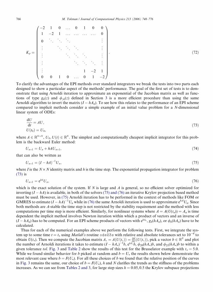
766 M. Tokman / Journal of Computational Physics 213 (2006) 748–776
Kp ¼
�2 1 0 . . . 0 1 0 0
1 �2 1 . . . . . . . . . . . . 0
0 . .. . .
. . .. ..
.
..
. . .. . .
. . .. ..
.
..
. . .. . .
. . .. ..
.
..
. . .. . .
. . .. ..
.
..
.1 �2 1
0 0 1 0 . . . 0 1 �2
0BBBBBBBBBBBBBBBBB@
1CCCCCCCCCCCCCCCCCA
. ð72Þ
To clarify the advantages of the EPI methods over standard integrators we break the tests into two parts eachdesigned to show a particular aspect of the methods� performance. The goal of the first set of tests is to dem-onstrate that using Arnoldi iteration to approximate an exponential of the Jacobian matrix as well as func-tions of type gk(z) and /ck(z) defined in Section 3 is a more efficient procedure than using the sameArnoldi algorithm to invert the matrix (I � hAn). To see how this relates to the performance of an EPI schemecompared to implicit methods consider a simple example of an initial value problem for a N-dimensionallinear system of ODEs:
dUdt
¼ AU ;
Uðt0Þ ¼ U 0;
ð73Þ
where A 2 RN�N , U 0;UðtÞ 2 RN . The simplest and computationally cheapest implicit integrator for this prob-lem is the backward Euler method:
Unþ1 ¼ Un þ hAUnþ1; ð74Þ
that can also be written as
Unþ1 ¼ ðI � hAÞ�1Un; ð75Þ
where I is the N · N identity matrix and h is the time step. The exponential propagation integrator for problem(73) is
Unþ1 ¼ ehAUn; ð76Þ
which is the exact solution of the system. If N is large and A is general, so no efficient solver optimized forinverting (I � hA) is available, in both of the solvers (75) and (76) an iterative Krylov projection based methodmust be used. However, in (75) Arnoldi iteration has to be performed in the context of methods like FOM orGMRES to estimate (I � hA)�1Un while in (76) the same Arnoldi iteration is used to approximate ehAUn. Sinceboth methods are A-stable the time step is not restricted by the stability requirement and the method with lesscomputations per time step is more efficient. Similarly, for nonlinear systems where A = A(U(tn)) = An is timedependent the implicit method involves Newton iteration within which a product of vectors and an inverse of(I � hAn) has to be computed. For an EPI scheme products of vectors with ehAn , gk(hAn), or /k(hAn) have to becalculated.
Thus for each of the numerical examples above we perform the following tests. First, we integrate the sys-tem up to some time t = t* using Matlab�s routine ode23s with relative and absolute tolerances set to 10�6 toobtain U(t*). Then we compute the Jacobian matrix A� ¼ AðUðt�ÞÞ ¼ DF
DUðUðt�ÞÞ, pick a vector b 2 RN and plotthe number of Arnoldi iterations it takes to estimate (I � hA*)
�1b, ehA�b, /20(hA*)b, and /21(hA*)b to within agiven tolerance tol. Fig. 3 and Table 2 show the results of this test for the Brusselator example with t* = 5.0.While we found similar behavior for b picked at random and b = U* the results shown below demonstrate themost relevant case where b = F(U*). For all these choices of b we found that the relative position of the curvesin Fig. 3 remains the same, our choice of b = F(U*), h and N clarifies the trends as the stiffness of the problemsincreases. As we can see from Tables 2 and 3, for large step sizes h = 0.05,0.5 the Krylov subspace projections
Fig. 3. We plot the 2-norm of the error in the Krylov subspace approximation of (i) (I � hA*)�1b using GMRES, (ii) (I � hA
*)�1b using
FOM, (iii) ehA�b, (iv) /20(hA*)b, and (v) /21(hA*
)b vs. the number of Arnoldi iterations it took to obtain this error for the BRUSS example.In these runs N = 200 and t
*= 5.0.
Table 2This table lists the number of Arnoldi iterations it took to approximate the expressions (i) (I � hA
*)�1b using GMRES, (ii) (I � hA
*)�1b
using FOM, (iii) ehA�b, (iv) /20(hA*)b, and (v) /21(hA*
)b for the Brusselator example to within tol = 10�5
Problem size, 2N (I � hA*)�1b via GMRES (I � hA
*)�1b via FOM ehA�b /20(hA*
)b /21(hA*)b
200 10 9 5 4 4400 21 18 8 4 4800 43 37 13 5 4
In this example h = 0.05, t*= 5, grid sizes N = 100,200,400, and b = F(U
*). Note that the Courant–Friedrichs–Levy (CFL) condition
restricted time steps corresponding to the grid sizes N = 100,200,400 are Dtstab = 1.22 · 10�3, 3.09 · 10�4, 7.77 · 10�5.
Table 3This table lists the number of Arnoldi iterations it took to approximate the expressions (i) (I � hA
*)�1b using GMRES, (ii) (I � hA
*)�1b
using FOM, (iii) ehA�b, (iv) /20(hA*)b, and (v) /21(hA*
)b for the Brusselator example to within tol = 10�5
In this example h = 0.5, t*= 5, grid sizes N = 100,200,400, and b = F(U
*).
M. Tokman / Journal of Computational Physics 213 (2006) 748–776 767
can be more efficiently used to complete the intermediate steps in EPI schemes (i.e., calculation of expressionsof type ehA�b, /20(hA*)b, and /21(hA*)b) compared to the intermediate steps that have to be performed withinthe Newton iteration of an implicit scheme (i.e., using Arnoldi iteration to approximate (I � hA*)
�1b). This
768 M. Tokman / Journal of Computational Physics 213 (2006) 748–776
trend remains the same as N or h increase and consequently the problems becomes more stiff (Fig. 3, Tables 2and 3).
Figs. 3–5 show plots of the 2-norm of the error vs. the corresponding number of Arnoldi iterations for dif-ferent time step sizes. We found that the relative positions of the curves do not change as the grid size N is
Fig. 4. These graphs plot the 2-norm of the error in the Krylov subspace approximation of (i) (I � hA*)�1b using GMRES, (ii)
(I � hA*)�1b using FOM, (iii) ehA�b, (iv) /20(hA*
)b, and (v) /21(hA*)b vs. the number of Arnoldi iterations it took to obtain this error for
the BURGERS example. For this calculation N = 1000, t*= 1.0.
Fig. 5. These graphs plot the 2-norm of the error in the Krylov subspace approximation of (i) (I � hA*)�1b using GMRES, (ii)
(I � hA*)�1b using FOM, (iii) ehA�b, (iv) /20(hA*
)b, and (v) /21(hA*)b vs. the number of Arnoldi iterations it took to obtain this error for
the CUSP example. In these runs N = 32,96, h = 5 · 10�5, t*= 10�5.
M. Tokman / Journal of Computational Physics 213 (2006) 748–776 769
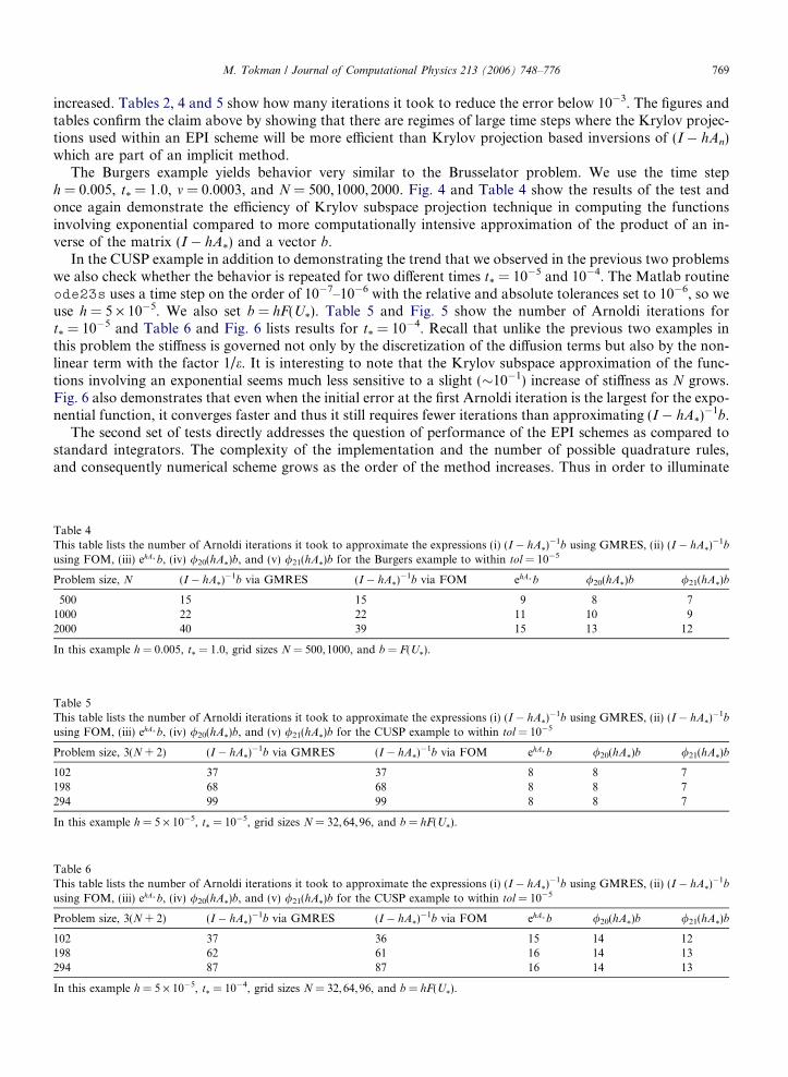
increased. Tables 2, 4 and 5 show how many iterations it took to reduce the error below 10�3. The figures andtables confirm the claim above by showing that there are regimes of large time steps where the Krylov projec-tions used within an EPI scheme will be more efficient than Krylov projection based inversions of (I � hAn)which are part of an implicit method.
The Burgers example yields behavior very similar to the Brusselator problem. We use the time steph = 0.005, t* = 1.0, m = 0.0003, and N = 500,1000,2000. Fig. 4 and Table 4 show the results of the test andonce again demonstrate the efficiency of Krylov subspace projection technique in computing the functionsinvolving exponential compared to more computationally intensive approximation of the product of an in-verse of the matrix (I � hA*) and a vector b.
In the CUSP example in addition to demonstrating the trend that we observed in the previous two problemswe also check whether the behavior is repeated for two different times t* = 10�5 and 10�4. The Matlab routineode23s uses a time step on the order of 10�7–10�6 with the relative and absolute tolerances set to 10�6, so weuse h = 5 · 10�5. We also set b = hF(U*). Table 5 and Fig. 5 show the number of Arnoldi iterations fort* = 10�5 and Table 6 and Fig. 6 lists results for t* = 10�4. Recall that unlike the previous two examples inthis problem the stiffness is governed not only by the discretization of the diffusion terms but also by the non-linear term with the factor 1/e. It is interesting to note that the Krylov subspace approximation of the func-tions involving an exponential seems much less sensitive to a slight (10�1) increase of stiffness as N grows.Fig. 6 also demonstrates that even when the initial error at the first Arnoldi iteration is the largest for the expo-nential function, it converges faster and thus it still requires fewer iterations than approximating (I � hA*)
�1b.The second set of tests directly addresses the question of performance of the EPI schemes as compared to
standard integrators. The complexity of the implementation and the number of possible quadrature rules,and consequently numerical scheme grows as the order of the method increases. Thus in order to illuminate
Table 4This table lists the number of Arnoldi iterations it took to approximate the expressions (i) (I � hA
*)�1b using GMRES, (ii) (I � hA
*)�1b
using FOM, (iii) ehA�b, (iv) /20(hA*)b, and (v) /21(hA*
In this example h = 5 · 10�5, t*= 10�4, grid sizes N = 32,64,96, and b = hF(U
*).
Fig. 6. These graphs plot the 2-norm of the error in the Krylov subspace approximation of (i) (I � hA*)�1b using GMRES, (ii)
(I � hA*)�1b using FOM, (iii) ehA�b, (iv) /20(hA*
)b, and (v) /21(hA*)b vs. the number of Arnoldi iterations it took to obtain this error for
the CUSP example. In these runs N = 32,96, h = 5 · 10�5, t*= 10�4.
770 M. Tokman / Journal of Computational Physics 213 (2006) 748–776
relative performance of explicit, implicit, and exponential methods we will compare the simplest second-ordermethods of each type. We will also show that even the third-order EPI schemes can be less costly than thesecond-order explicit and implicit integrators. In these tests we integrate each of the three examples aboveusing the following methods.
AB2 is the second-order explicit Adams–Bashforth method
Unþ1 ¼ Un þh2ð3F n � F n�1Þ. ð77Þ
Since the method is two-step we use the second-order Runge–Kutta (Midpoint) method to obtain the startingvalues for the scheme. Obviously, AB2 requires the least amount of computations per time step out of all themethods we test but the time step of this method is limited by the stability requirement.
AM2 is the second-order implicit Adams–Moulton method (or Trapezoidal rule)
Unþ1 ¼ Un þh2ðF n þ F nþ1Þ. ð78Þ
It is well known that this method is A-stable and therefore the time step size is only restricted by accuracy.However, since system (78) is nonlinear the good stability properties of this method come at the expense ofan increase in the number of computations per time step. Thus at each time step we will employ a Newtonmethod to solve for Un + 1 and a Krylov subspace projection method, GMRES, to invert the matrixðI � ðh=2ÞDFDUðUÞÞ within each Newton iteration. Therefore at each time step the number of Newton iterationsrequired to achieve a given tolerance is equal to the number of times the Arnoldi algorithm has to be executed.
EPI2 is the second-order multistep type EPI scheme
Unþ1 ¼ Un þ g ðAnhÞhF n; ð79Þ
0
M. Tokman / Journal of Computational Physics 213 (2006) 748–776 771
where g0(z) = (ez � 1)/z. Out of all possible second -order exponential propagation schemes this methodrequires the least amount of computation per times step since only one evaluation of F(U) and one Krylovprojection have to be performed.
EPI3: this third-order multistep type EPI method was introduced in Section 3.2.1:
TableThis tawith a
Time s
10�4
2 · 10�
4 · 10�
8 · 10�
1.6 · 13.2 · 16.4 · 11.28 ·2.56 ·5.12 ·1.024 ·
In thes
Unþ1 ¼ Un þ g0ðAnhÞhF n þ2
3g1ðAnhÞhRn�1; ð80Þ
where
g0ðzÞ ¼ez � 1
z;
g1ðzÞ ¼ez � ð1þ zÞ
z2.
ð81Þ
This two step method requires at most one evaluation of F(U) (the value of Fn � 1 can be saved from the pre-vious time step) and two Krylov subspace projections to compute g0(Ahh)hFn and g1(Anh)hRn � 1 at each timestep. As noted earlier, in general if the residuals allow to do so, it is possible to optimize the scheme by reusingthe Krylov basis from the evaluation of g0(Ahh)hFn to calculate g1(Anh)hRn � 1. However, in this implementa-tion we consider the worst case scenario and perform two Krylov projections at each time step.
EPIRK3: this third-order Runge–Kutta type EPI method was introduced in Section 3.2.2 and is given by
r1 ¼ Un þ 2/20ðAnh2Þ h2F n;
Unþ1 ¼ Un þ /20ðAnhÞhF n þ1
3/21ðAnhÞhRðr1Þ;
ð82Þ
where
/20ðzÞ ¼ez � 1
z;
/21ðzÞ ¼ 2ez � ð1þ zÞ
z2.
ð83Þ
This method has about the same operations count per time step as the scheme EPI3 above plus one additionalfunction evaluation F(r1). Note that only one Krylov projection is needed to compute both /20(Anh/2)(h/2)Fn
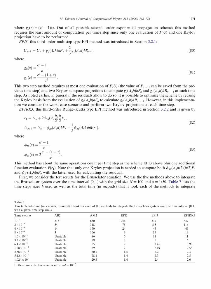
and /20(Anh)hFn with the latter used for calculating the residual.First, we consider the test results for the Brusselator equation. We use the five methods above to integrate
the Brusselator system over the time interval [0,1] with the grid size N = 100 and a = 1/50. Table 7 lists thetime steps sizes h used as well as the total time (in seconds) that it took each of the methods to integrate
7ble lists time (in seconds, rounded) it took for each of the methods to integrate the Brusselator system over the time interval [0,1]given time step size h
Fig. 7. The graphs show the 2-norm of the error vs. the time step size h for integration of the Brusselator system with methods AM2, EPI2,EPI3, and EPIRK3. In these runs the tolerance is set to tol = 10�7.
772 M. Tokman / Journal of Computational Physics 213 (2006) 748–776
the system over the given time interval. In these calculations the tolerance used for both the Newton iterationas well as for all Krylov projections is set to 10�7. Fig. 7 shows the 2-norm of the corresponding errors whichare calculated using the solution computed with Matlab�s ode15s routine with 10�13 relative and absolutetolerances as reference. Note that while for large values of the time step the graphs in Fig. 7 exhibit the ex-pected order of the methods, for small values of the time step the graphs for schemes EPI3 and EPIRK3 showa curious peak in error (Fig. 7). This is explained by looking at the results of the same calculations with thelowered tolerance of tol = 10�9 in Figs. 8(a) and (b). As we can see from these graphs the peak is shifted tothe left. The reason for this phenomenon is that in the range of time step values where the peak is located theglobal error is dominated by the error of the Krylov subspace approximations. When the tolerance is loweredand the exponential functions are computed with more precision the time discretization error prevails in thisrange as can by see by comparing Figs. 7(a) and (b) and 8(a) and (b). In either of these cases, however, theexponential propagation schemes are shown to be more efficient than the implicit Trapezoidal Rule methodAM2 as can be seen from the results in Table 7 and more efficient than the explicit method AB2 whichbecomes unstable for time steps larger than h � 0.0012.
Let us also examine the effect the magnitude of the tolerances has on the comparative performance of theimplicit and EPI methods above. For this test we are interested in the large time step regimes and therefore weset h = 0.0512. Since very loose tolerances are used sometimes in the Krylov projections step of a Newton–Krylov method to improve efficiency, we will vary the value of tol and record the integration time and theerror for the schemes AM2, EPI2, EPI3, and EPIRK3. First, we tried to lower the tolerance on the Krylovprojection step in AM2 but leave the tolerance for the outer Newton iteration at tol = 10�6. However, we
Fig. 8. The graphs show the 2-norm of the error vs. the time step size h for integration of the Brusselator system with methods AM2, EPI2,EPI3 and EPIRK3. In these runs the tolerance is set to tol = 10�9.
M. Tokman / Journal of Computational Physics 213 (2006) 748–776 773
found that in this case the Newton iteration in AM2 stops converging and the solution cannot be obtained.Thus we ran tests where the tolerances for both the Krylov projections and the Newton iteration are set to arange of values tol = 10�3,10�4,10�5. The AM2 algorithm consists of a straightforward implementation of theNewton–Krylov iteration with fixed values of tolerances for both the Newton and Krylov iterations. Suchimplementation provides the most direct way to compare the implicit and EPI methods. However, the Newtonmethod has existed for a long time and various improvements to the basic algorithm has been developed. Inparticular, for large systems an inexact Newton iteration has been introduced and shown to be more cost effi-cient for many problems [37]. In the future it might be possible to develop similar improvements for the EPImethods. If so comparing such improved EPI schemes with the implicit scheme with inexact Newton methodwould be more fair. However, for the sake of completeness we have also implemented and included in ourcomparison study a version of the implicit Adams–Moulton method with embedded inexact Newton methodas it is described in [38]. The inexact Newton iteration replaces the original algorithm for solving G(x) = 0 withiteration xk + 1 = xk + sk where G 0(xk)sk = � G(xk) + rk, k = 1,2, . . . and rk satisfies condition iG(xk) +G 0(xk)ski 6 gkiG(xk)i. Thus to fully specify an inexact Newton algorithm one has to choose the forcing termgk. We follow [38] and choose gk to be
TableThis taeach o
Metho
AM2AM2INEPI2EPI3EPIRK
The to
TableThis tasize h
Time s
10�4
2 · 10�
4 · 10�
8 · 10�
1.6 · 13.2 · 16.4 · 1
In thes
gk ¼kGðxkÞ � Gðxk�1Þ � G0ðxk�1Þsk�1k
kGðxk�1Þk. ð84Þ
Table 8 summarizes the results of these tests. As we can see even for low tolerances the EPI schemes still out-perform the implicit method both in speed and in the accuracy of the obtained solution. In fact, the EPIschemes also outperform the implicit method AM2IN although by a smaller compared to AM2. While thegoal of this paper is primarily to introduce EPI schemes and demonstrate their performance, further fine tun-ing of these methods and comparisons with other state-of-the-art implicit algorithms will be addressed in ourfuture work.
As we can see from Table 9 and Fig. 9 performance of the methods for the BURG example is very similar tothe case of the Brusselator system. Parameters used for the Burgers equation were the grid size N = 500,
8ble compares performance of the methods AM2, AM2IN, EPI2, EPI3 and EPIRK3 with respect to different values of tolerance; inf the tests the Brusselator system was integrated up to time t = 1 with N = 100 and h = 0.0512
Fig. 9. The graphs show the 2-norm of the error vs. the time step size h for integration of the BURG system with methods AM2, EPI2,EPI3, and EPIRK3. In these runs the tolerance is set to tol = 10�7.
Table 10The table shows results of the comparison of the methods for integrating the CUSP example over the time interval [0,10�4] with time stepsh = 10�5 and h = 5 · 10�6
h = 1E � 5 Execution time Error h = 5E � 6 Execution time Error
774 M. Tokman / Journal of Computational Physics 213 (2006) 748–776
m = 3 · 10�4, the time interval [0,0.5] and the tolerance tol = 10�7. A slight difference with the Brusselatorexample is that in this case it appears that an explicit method is more efficient than any other technique. How-ever, as N increases and so does the stiffness the stability bound becomes severely restrictive, while as we cansee from the table the EPI schemes remain efficient at high values of h. The results of the table also clearlyindicate the superior efficiency of the EPI schemes compared to the implicit solver AM2.
In the CUSP example the methods exhibit a different behavior which is instructive to consider. We performthe calculations with grid size N = 32, parameter values e = 10�4, r = 1/144, tol = 10�7 over the time interval[0,10�4]. Here we find that the accuracy considerations outweigh those of stability (Table 10). The stabilitybound on the time step for the explicit scheme AB2 in this case is of the order 10�5. For time steps smallerthan this bound the comparison of the total time of integration of the CUSP system by implicit and EPIschemes shows the same results as for the previous two examples. The errors in this case are also comparableeven though the exponential propagation schemes give a somewhat larger error. However, when the time stepexceeds the stability bound we find that not only AB2 goes unstable, but the Newton iteration within the im-plicit method AM2 no longer converges to within a given tolerance and the EPI schemes also yield unreason-ably large errors. Thus for this problem an explicit method will always be the fastest way to compute thesolution as confirmed by our numerical experiments and integration with either implicit or exponential prop-agation schemes is not appropriate.
5. Conclusions
In this paper, we have introduced a new class of exponential integrators which we called exponential prop-agation iterative (EPI) methods. We have discussed the methodology for the construction of these schemesand studied their performance on several test problems. We have demonstrated that the faster convergenceof Arnoldi iterations needed by EPI schemes provide computational savings compared to standard implicitNewton–Krylov integrators with no preconditioning. It is not clear at this point whether EPI schemes canbe used in conjunction with a preconditioner and we plan to investigate this question in the future. We have
M. Tokman / Journal of Computational Physics 213 (2006) 748–776 775
also showed the superior stability properties of these methods compared to explicit schemes. Thus the EPIschemes can provide an efficient alternative to standard integrators if no good preconditioner is availablefor a large-scale stiff problem, its time integration is challenging because of a stability bound on the time stepand the accuracy requirement allows a time step far exceeding that bound, While the numerical examples inthis paper provide some guidance as to what type of problems can benefit from the use of EPI schemes moreresearch is needed to determine the classes of systems for which the EPI methods are advantageous. The studyof the performance and application of the higher-order EPI methods proposed in this paper will be presentedelsewhere.
Acknowledgments
The author thanks Prof. Alexandre Chorin and Prof. G.I. Barenblatt for introducing her to an inspiringand supportive scientific environment, Prof. Ole Hald and Dr. David Bernstein for helpful discussions, andMr. John Barber for advice on Mathematica software. This work was supported in part by the NSF VIGREGrant DMS-9819728, NSF/DOE partnership in plasma physics Grant DMS-0317511, and University of Cal-ifornia President�s Postdoctoral Fellowship Program.
References
[1] D.A. Knoll, D.E. Keyes, Jacobian-free Newton–Krylov methods: a survey of approaches and applications, J. Comput. Phys. 193(2004) 357–397.
[2] E. Hairer, S.P. Nørsett, G. Wanner, Solving Ordinary Differential Equations, Springer, Berlin, 1987.[3] S.M. Cox, Exponential time differencing (ETD) references. Available from: <www.maths.adelaide.edu.au/people/scox/etd.html>.[4] J. Certaine, The solution of ordinary differential equations with large time constants, in: A. Ralston, H.S. Wilf (Eds.), Mathematical
Methods for Digital Computers, 1960, pp. 128–132.[5] D.A. Pope, An exponential method of numerical integration of ordinary differential equations, Commun. ACM 6 (8) (1963) 491–493.[6] J.D. Lawson, Generalized Runge–Kutta processes for stable systems with large Lipschitz constants, SIAM J. Numer. Anal. 4 (1967)
372–380.[7] S.P. Nørsett, An A-stable modification of the Adams–Bashforth methods, Lecture Notes Math. 109 (1969) 214–219.[8] C.B. Moler, C.F. Van Loan, Nineteen dubious ways to compute the exponential of a matrix, SIAM Rev. 20 (4) (1978) 801–836.[9] C.B. Moler, C.F. Van Loan, Nineteen dubious ways to compute the exponential of a matrix, twenty-five years later, SIAM Rev. 45 (1)
(2003) 3–49.[10] E. Gallopoulos, Y. Saad, Efficient solution of parabolic equations by Krylov approximation methods, SIAM J. Sci. Stat. Comp. 13
(1992) 1236–1264.[11] J.D. Lawson, S.J. Thomas, R.V.M. Zahar, Weighted quadrature in Krylov methods, Utilitas Mathematica 51 (1997) 165–182.[12] G. Beylkin, J.M. Keiser, L. Vozovoi, A new class of time discretization schemes for the solution of nonlinear PDEs, J. Comput. Phys.
147 (1998) 362–387.[13] S.M. Cox, P.C. Matthews, Exponential time differencing for stiff systems, J. Comput. Phys. 176 (2002) 430–455.[14] A.K. Kassam, L.N. Trefethen, Fourth-order time stepping for stiff PDEs, SIAM J. Sci. Comp. (2004).[15] S. Krogstad, Generalized integrating factor methods for stiff PDEs, J. Comput. Phys. 203 (1) (2005) 72–88.[16] M. Hochbruck, A. Ostermann, Exponential Runge–Kutta methods for parabolic problems, Appl. Numer. Math. 53 (2005) 323–339.[17] Y. Saad, Iterative Methods for Sparse Linear Systems, PWS Publishing Company, 1996.[18] C.W. Gear, Y. Saad, Iterative solution of linear equations in ODE codes, SIAM J. Sci. Stat. Comput. 4 (4) (1983) 583–601.[19] A. Nauts, R.E. Wyatt, New approach to many-state quantum dynamics: the recursive-residue-generation method, Phys. Rev. Lett. 51
(5) (1983) 2238–2241.[20] T.J. Park, J.C. Light, Unitary quantum time evolution by iterative Lanczos reduction, J. Chem. Phys. 85 (1986) 5870–5876.[21] H.A. Van der Vorst, An iterative solution method for solving f(a)x = b using Krylov subspace information obtained for the symmetric
positive definite matrix a, J. Comput. Appl. Math. 18 (1987) 249–263.[22] R.A. Friesner, L.S. Tuckerman, B.C. Dornblaser, T.V. Russo, A method for exponential propagation of large systems of stiff
nonlinear differential equations, J. Sci. Comput. 4 (1989) 327–354.[23] M. Tokman, Magnetohydrodynamic modeling of solar coronal arcades using exponential propagation methods, Ph.D. Thesis,
Caltech, 2000.[24] M. Hochbruck, Ch. Lubich, On Krylov subspace approximations to the matrix exponential operator, SIAM J. Numer. Anal. 34
(1997) 1911–1925.[25] M. Hochbruck, Ch. Lubich, H. Selhofer, Exponential integrators for large systems of differential equations, SIAM J. Sci. Comput. 19
(1998) 1552–1574.[26] M. Tokman, P.M. Bellan, Three-dimensional model of the structure and evolution of coronal mass ejections, Astrophys. J. 567 (2)
776 M. Tokman / Journal of Computational Physics 213 (2006) 748–776
[27] W.E. Arnoldi, The principle of minimized iteration in the solution of the matrix eigenvalue problem, Quart. Appl. Math. 9 (1951) 17–29.
[28] L.A. Knizhnerman, Calculation of functions of unsymmetric matrices using Arnoldi method, Comput. Math. Math. Phys. 31 (1)(1991) 1–9.
[29] Y. Saad, Analysis of some Krylov subspace approximations to the matrix exponential operator, SIAM J. Numer. Anal. 29 (1992)209–228.
[30] R.B. Sidje, Expokit: a software package for computing matrix exponentials, ACM T. Math. Software 24 (1) (1998) 130–156.[31] R.H. Merson, An operational method for the study of integration processes, in: Proceedings of the Symposium on Data Processing,
Weapons Research Establishment, Salisbury, Australia, 1957, pp. 110-1–110-25.[32] J.C. Butcher, Coefficients for the study of Runge–Kutta integration processes, J. Austr. Math. Soc. 3 (1963) 185–201.[33] R. Lefever, G. Nicolis, Chemical instabilities and sustained oscillations, J. Theor. Biol. 30 (1971) 267–284.[34] R. FitzHugh, Mathematical models of excitation and propagation in nerve, in: H.P. Schwan (Ed.), Biological Engineering, McGraw-
Hill, New York, 1969, pp. 1–85.[35] J. Nagumo, S. Arimoto, S. Yoshizawa, An active pulse transmission line simulating nerve axon, Proc. IRE 50 (1962) 2061–2070.[36] E.C. Zeeman, Differential equations for the heartbeat and nerve impulse, in: C.H. Waddington (Ed.), Towards a Theoretical Biology,
vol. 4, Edinburgh University press, 1972, pp. 8–67.[37] R.S. Dembo, S.C. Eisenstat, T. Steihaug, Inexact Newton methods, SIAM J. Numer. Anal. 19 (2) (1982) 400–408.[38] S.C. Eisenstat, H.F. Walker, Choosing the forcing terms in an inexact Newton method, SIAM J. Sci. Comput. 17 (1) (1996) 16–32.