Ecography E7773Roquet, C., Thuiller, W. and Lavergne, S. 2012. Building megaphylogenies for macroecology: taking up the challenge. – Ecography 35: xxx–xxx.

Supplementary material

  1  

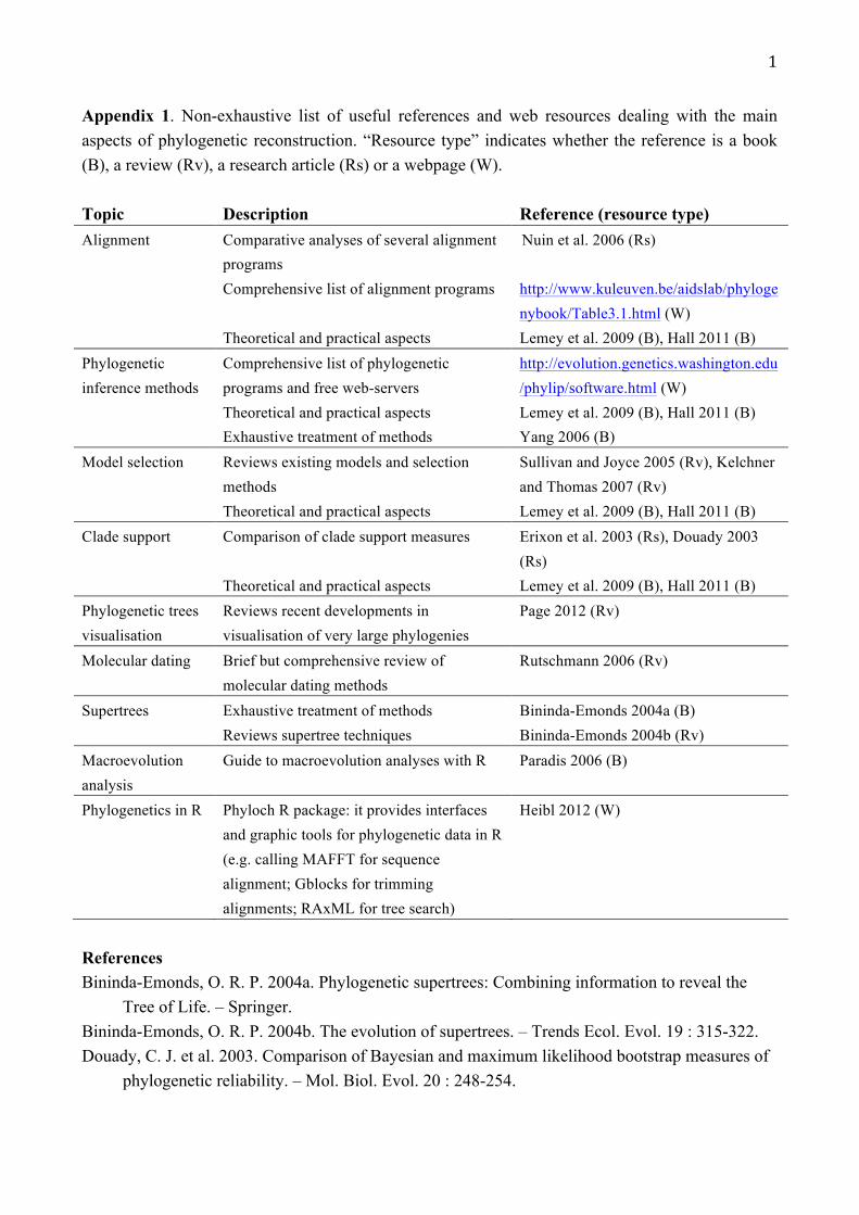
Appendix 1. Non-exhaustive list of useful references and web resources dealing with the main aspects of phylogenetic reconstruction. “Resource type” indicates whether the reference is a book (B), a review (Rv), a research article (Rs) or a webpage (W). Topic Description Reference (resource type) Alignment Comparative analyses of several alignment

programs Nuin et al. 2006 (Rs)

Comprehensive list of alignment programs http://www.kuleuven.be/aidslab/phylogenybook/Table3.1.html (W)

Theoretical and practical aspects Lemey et al. 2009 (B), Hall 2011 (B) Phylogenetic inference methods

Comprehensive list of phylogenetic programs and free web-servers

http://evolution.genetics.washington.edu/phylip/software.html (W)

Theoretical and practical aspects Exhaustive treatment of methods

Lemey et al. 2009 (B), Hall 2011 (B) Yang 2006 (B)

Model selection Reviews existing models and selection methods

Sullivan and Joyce 2005 (Rv), Kelchner and Thomas 2007 (Rv)

Theoretical and practical aspects Lemey et al. 2009 (B), Hall 2011 (B) Clade support Comparison of clade support measures Erixon et al. 2003 (Rs), Douady 2003

(Rs) Theoretical and practical aspects Lemey et al. 2009 (B), Hall 2011 (B) Phylogenetic trees visualisation

Reviews recent developments in visualisation of very large phylogenies

Page 2012 (Rv)

Molecular dating Brief but comprehensive review of molecular dating methods

Rutschmann 2006 (Rv)

Supertrees Exhaustive treatment of methods Bininda-Emonds 2004a (B) Reviews supertree techniques Bininda-Emonds 2004b (Rv) Macroevolution analysis

Guide to macroevolution analyses with R Paradis 2006 (B)

Phylogenetics in R Phyloch R package: it provides interfaces and graphic tools for phylogenetic data in R (e.g. calling MAFFT for sequence alignment; Gblocks for trimming alignments; RAxML for tree search)

Heibl 2012 (W)

References Bininda-Emonds, O. R. P. 2004a. Phylogenetic supertrees: Combining information to reveal the

Tree of Life. – Springer. Bininda-Emonds, O. R. P. 2004b. The evolution of supertrees. – Trends Ecol. Evol. 19 : 315-322. Douady, C. J. et al. 2003. Comparison of Bayesian and maximum likelihood bootstrap measures of

phylogenetic reliability. – Mol. Biol. Evol. 20 : 248-254.

  2  

Erixon, P. et al. 2003. Reliability of Bayesian posterior probabilities and bootstrap frequencies in phylogenetics. – Syst. Biol. 52: 665-73.

Hall, B. G. 2011. Phylogenetic Trees Made Easy: A How - To Manual, 4th edition. – Sinauer Associates.

Heibl, C. 2012. Tools for phylogenetics and taxonomy. http://www.christophheibl.de/Rpackages.html

Kelchner, S. A. and Thomas, M. A. 2007. Model use in phylogenetics : nine key questions. – Trends Ecol. Evol. 22 : 87-94.

Lemey, P. et al. 2009. The Phylogenetic Handbook: A Practical Approach to Phylogenetic Analysis and Hypothesis Testing. – Cambridge University Press.

Nuin, P. A. S. et al. 2006. The accuracy of several multiple sequence alignment programs for proteins. – BMC Bioinformatics 7: 471.

Page, R. D. M. Space, time, form : viewing the Tree of Life. – Trends Ecol. Evol. 27 : 113-120. Paradis, E. 2006. Analysis of Phylogenetics and Evolution with R. - Springer-Verlag. Rutschmann, F. 2006. Molecular dating of phylogenetic trees : a brief review of current methods

that estimate divergence times. – Diversity Distrib. 12 : 35-48. Sullivan, J. and Joyce, P. 2005. Model selection in phylogenetics. – Annu. Rev. Ecol. Evol. Syst.

36 : 445-466. Yang, Z. 2006. Computational Molecular Evolution. – Oxford Series in Ecology and Evolution.

Appendix 2. Detailed protocol to build megaphylogenies

Cristina Roquet, Wilfried Thuiller and Sebastien Lavergne

June 27, 2012

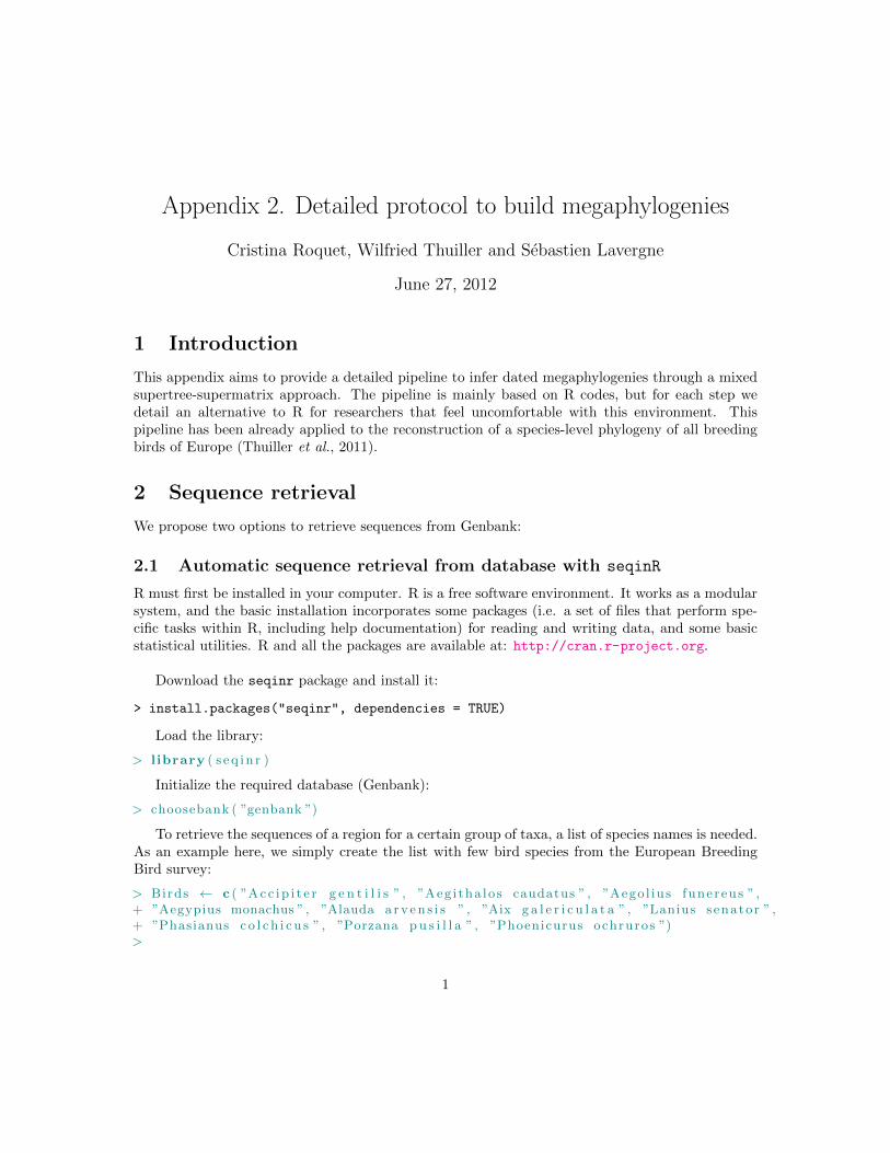
1 Introduction

This appendix aims to provide a detailed pipeline to infer dated megaphylogenies through a mixedsupertree-supermatrix approach. The pipeline is mainly based on R codes, but for each step wedetail an alternative to R for researchers that feel uncomfortable with this environment. Thispipeline has been already applied to the reconstruction of a species-level phylogeny of all breedingbirds of Europe (Thuiller et al., 2011).

2 Sequence retrieval

We propose two options to retrieve sequences from Genbank:

2.1 Automatic sequence retrieval from database with seqinR

R must first be installed in your computer. R is a free software environment. It works as a modularsystem, and the basic installation incorporates some packages (i.e. a set of files that perform spe-cific tasks within R, including help documentation) for reading and writing data, and some basicstatistical utilities. R and all the packages are available at: http://cran.r-project.org.

Download the seqinr package and install it:

> install.packages("seqinr", dependencies = TRUE)

Load the library:

> l ibrary ( s e q i n r )

Initialize the required database (Genbank):

> choosebank ( ”genbank ”)

To retrieve the sequences of a region for a certain group of taxa, a list of species names is needed.As an example here, we simply create the list with few bird species from the European BreedingBird survey:

> Birds ← c ( ”Acc i p i t e r g e n t i l i s ” , ”Aeg i tha lo s caudatus ” , ”Aego l ius funereus ” ,+ ”Aegypius monachus ” , ”Alauda a rv en s i s ” , ”Aix g a l e r i c u l a t a ” , ”Lanius senator ” ,+ ”Phasianus c o l c h i c u s ” , ”Porzana p u s i l l a ” , ”Phoenicurus ochruros ”)>

1

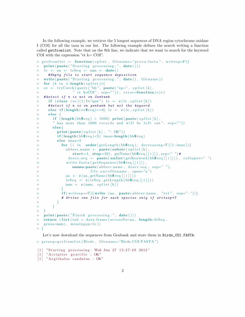
In the following example, we retrieve the 5 longest sequences of DNA region cytochrome oxidaseI (COI) for all the taxa in our list. The following example defines the search writing a functioncalled getfromlist. Note that on the 9th line, we indicate that we want to search for the keywordCOI with the expression ”et k= COI”:

> g e t f r om l i s t ← function ( s p l i s t , f i l ename=”p rova . f a s t a ” , wr i t e sp=F){+ print (paste ( ”S ta r t i ng p ro c e s s i ng : ” , date ( ) ) )+ l e ← aa ← l eSeq ← nam ← date ( )+ #Empty file to start sequence deposition

+ write (paste ( ”S ta r t i ng p ro c e s s i ng : ” , date ( ) , f i l ename ) )+ for ( k in 1 : length ( s p l i s t ) ){+ ee ← tryCatch ( query ( ”bb ” , paste ( ”sp=”, s p l i s t [ k ] ,+ ” et k=COI ” , sep=””) ) , e r r o r=function ( e ) e )+ #detect if n is not on Genbank

+ i f ( class ( ee ) [ 1 ] !=”qaw ”) l e ← c ( l e , s p l i s t [ k ] )+ #detect if n is on genbank but not the keyword

+ else i f ( length ( ee$ req )==0) l e ← c ( l e , s p l i s t [ k ] )+ else {+ i f ( length (bb$ req ) > 1000) print (paste ( s p l i s t [ k ] ,+ ” has more than 1000 r e co rd s and w i l l be l e f t out ” , sep=””) )+ else {+ print (paste ( s p l i s t [ k ] , ”: OK”) )+ i f ( length (bb$ req )<5) imax=length (bb$ req )+ else imax=5+ for ( i in order ( getLength (bb$ req ) , de c r ea s ing=T) [ 1 : imax ] ) {+ abbrev.name ← paste ( substr ( s p l i s t [ k ] ,+ start=1, stop=20) , getName (bb$ req [ [ i ] ] ) , sep=” ”)#+ de s c r . s e q ← paste ( unlist ( getKeyword (bb$ req [ [ i ] ] ) ) , c o l l a p s e=” ”)+ w r i t e . f a s t a ( getSequence (bb$ req [ [ i ] ] ) ,+ names=paste ( abbrev.name , de s c r . s eq , sep=” ”) ,+ f i l e . o u t=f i l ename , open=”a ”)+ aa ← c ( aa , getName (bb$ req [ [ i ] ] ) )+ leSeq ← c ( leSeq , getLength (bb$ req [ [ i ] ] ) )+ nam ← c (nam, s p l i s t [ k ] )+ }+ i f ( wr i t e sp==T){write ( aa , paste ( abbrev.name , ”txt ” , sep=”. ”) )}+ # Writes one file for each species only if writesp=T

+ }+ }+ }+ print (paste ( ”F in i sh p ro c e s s i ng : ” , date ( ) ) )+ return ( l i s t ( tab = data . f rame ( accessNo=aa , length=leSeq ,+ genus=nam) , miss ingsp=l e ) )+ }

Let’s now download the sequences from Genbank and store them in Birds_COI.FASTA:

> get seq=g e t f r om l i s t ( Birds , f i l ename=”Birds COI.FASTA ”)

[ 1 ] ”S ta r t i ng p ro c e s s i ng : Wed Jun 27 15 : 27 : 49 2012 ”[ 1 ] ”Acc i p i t e r g e n t i l i s : OK”[ 1 ] ”Aeg i tha lo s caudatus : OK”

2

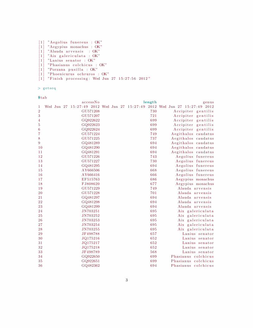
[ 1 ] ”Aego l ius funereus : OK”[ 1 ] ”Aegypius monachus : OK”[ 1 ] ”Alauda a rv en s i s : OK”[ 1 ] ”Aix g a l e r i c u l a t a : OK”[ 1 ] ”Lanius senator : OK”[ 1 ] ”Phasianus c o l c h i c u s : OK”[ 1 ] ”Porzana p u s i l l a : OK”[ 1 ] ”Phoenicurus ochruros : OK”[ 1 ] ”F in i sh p ro c e s s i ng : Wed Jun 27 15 : 27 : 56 2012 ”

> get seq

$tabaccessNo length genus

1 Wed Jun 27 15 : 27 : 49 2012 Wed Jun 27 15 : 27 : 49 2012 Wed Jun 27 15 : 27 : 49 20122 GU571208 730 Acc i p i t e r g e n t i l i s3 GU571207 721 Acc i p i t e r g e n t i l i s4 GQ922622 699 Acc i p i t e r g e n t i l i s5 GQ922623 699 Acc i p i t e r g e n t i l i s6 GQ922624 699 Acc i p i t e r g e n t i l i s7 GU571224 749 Aeg i tha lo s caudatus8 GU571225 737 Aeg i tha lo s caudatus9 GQ481289 694 Aeg i tha lo s caudatus10 GQ481290 694 Aeg i tha lo s caudatus11 GQ481291 694 Aeg i tha lo s caudatus12 GU571226 743 Aego l ius funereus13 GU571227 730 Aego l ius funereus14 GQ481295 694 Aego l ius funereus15 AY666506 668 Aego l ius funereus16 AY666416 666 Aego l ius funereus17 EF515763 686 Aegypius monachus18 FJ808620 677 Aegypius monachus19 GU571229 749 Alauda a rv en s i s20 GU571228 701 Alauda a rv en s i s21 GQ481297 694 Alauda a rv en s i s22 GQ481298 694 Alauda a rv en s i s23 GQ481299 694 Alauda a rv en s i s24 JN703251 695 Aix g a l e r i c u l a t a25 JN703252 695 Aix g a l e r i c u l a t a26 JN703253 695 Aix g a l e r i c u l a t a27 JN703254 695 Aix g a l e r i c u l a t a28 JN703255 695 Aix g a l e r i c u l a t a29 JF498788 657 Lanius senator30 JQ175216 652 Lanius senator31 JQ175217 652 Lanius senator32 JQ175218 652 Lanius senator33 JF498789 568 Lanius senator34 GQ922650 699 Phasianus c o l c h i c u s35 GQ922651 699 Phasianus c o l c h i c u s36 GQ482362 694 Phasianus c o l c h i c u s

3

37 GQ482363 694 Phasianus c o l c h i c u s38 GQ482364 694 Phasianus c o l c h i c u s39 JQ342131 914 Porzana p u s i l l a40 JQ342132 914 Porzana p u s i l l a41 GU571546 751 Phoenicurus ochruros42 GQ482384 694 Phoenicurus ochruros43 GQ482385 694 Phoenicurus ochruros44 GQ482386 694 Phoenicurus ochruros45 GQ482387 694 Phoenicurus ochruros

$miss ingsp[ 1 ] ”Wed Jun 27 15 : 27 : 49 2012 ”

Once the search is finished, getseq contains the list of accession numbers and the length ofsequences retrieved for each taxa, and the missing taxa. At the end of the search we will obtain aFASTA file (see below) containing all the sequences retrieved. It is a good idea to repeat the queryseveral times with different search terms for the region(s) of interest, because databases such asGenbank are only partly standardized. When composing queries, the symbol @ can be used as awild card for any string of characters at the end of the search term.

2.2 Manual sequence retrieval from database with Geneious

Those who do not feel comfortable with R can retrieve sequences by hand, which will take longer.Geneious is a program with a nice-user interface that makes the retrieval easier and quicker thanretrieving directly the sequences from the Genbank webpage. Geneious Basic (available for allplatforms) is free and can be downloaded from http://www.geneious.com/download. Open theprogram and select Nucleotide under the NCBI menu on the left-side framework, the Source Panel.Introduce your parameters of search using the flags available (e.g. Organism and keyword) and runthe search, the symbol * can be used as a wild card. When results are returned, order the sequencesretrieved by length, select the ones of interest and drag them to a folder on the left framework,under the Local menu. Repeat the process for each taxon, go to the folder where you dragged allthe sequences, and export all together to a unique FASTA file by clicking on Export under the Filemenu.

3 Common formats of sequence and alignment files

We briefly present here the 3 most common formats. The format can easily be changed to anotherone with the program Readseq (Gilbert 2001), which is able to read almost all the existing typesof alignment file formats, and available at the free web-server http://www.ebi.ac.uk/cgi-bin/

readseq.cgi.

3.1 FASTA

The FASTA format is the simplest one: it begins with a single-line sequence description precededby >; the next line contains the sequence. If the sequence is aligned, gaps are indicated with -.Almost all phylogenetic programs can read or import this type of file:

4

>Taxon1AAATTTGGCCGGTTAAATTGGAACCCCTTATGCCATAGCCTTGCCAATGCGTCAACCCAATTGCAACA>Taxon2AATTATATCCGCTTAACCTGGAATTCCTGATGCCGGAGCCTTGCAAATGCGTTAACCCAATTGCCACA>Taxon3AATTATGCCAGGTTATATGAGAACCCCTGGTGCCAGGACCTTGCCAATGCGTAAACTCAATTGCAACA

3.2 PHYLIP

The first line of the input file contains the number of taxa and the number of sequence charactersseparated by a blank. The taxon name needs to be restricted to ten characters. The name hasto be on the same line as the first character of the sequence for that taxon. The PHYLIP formatcan be interleaved or sequential. In sequential format, all the information of one sequence is givenbefore the next starts:

3 68Taxon1 AAATTTGGCCGGTTAAATTGGAACCCCTTATGCCATAGCCTTGCCAATGCGTCAACCCAATTGCAACATaxon2 AATTATATCCGCTTAACCTGGAATTCCTGATGCCGGAGCCTTGCAAATGCGTTAACCCAATTGCCACATaxon3 AATTATGCCAGGTTATATGAGAACCCCTGGTGCCAGGACCTTGCCAATGCGTAAACTCAATTGCAACA

In interleaved format, the first part of the file contains the first part of each of the sequences,then optionally a line containing nothing but a carriage-return character, then the second part ofeach sequence, and so on. Only the first parts of the sequences are preceded by names:

3 68Taxon1 AAATTTGGCCGGTTAAATTGGAACCCCTTATGCCATAGCCTTGCCAATGCTaxon2 AATTATATCCGCTTAACCTGGAATTCCTGATGCCGGAGCCTTGCAAATGCTaxon3 AATTATGCCAGGTTATATGAGAACCCCTGGTGCCAGGACCTTGCCAATGCGTCAACCCAATTGCAACAGTTAACCCAATTGCCACAGTAAACTCAATTGCAACA

3.3 NEXUS

A Nexus file must begin with the string #NEXUS in the first line. This is a modular format and cancontain both sequence data and phylogenetic trees in block units (Maddison et al., 1997). Eachblock starts with Begin block_name; and finishes with End;. Comments can be added in the fileusing [ ]. The sequences block is called DATA, and some information must be specified at the be-

5

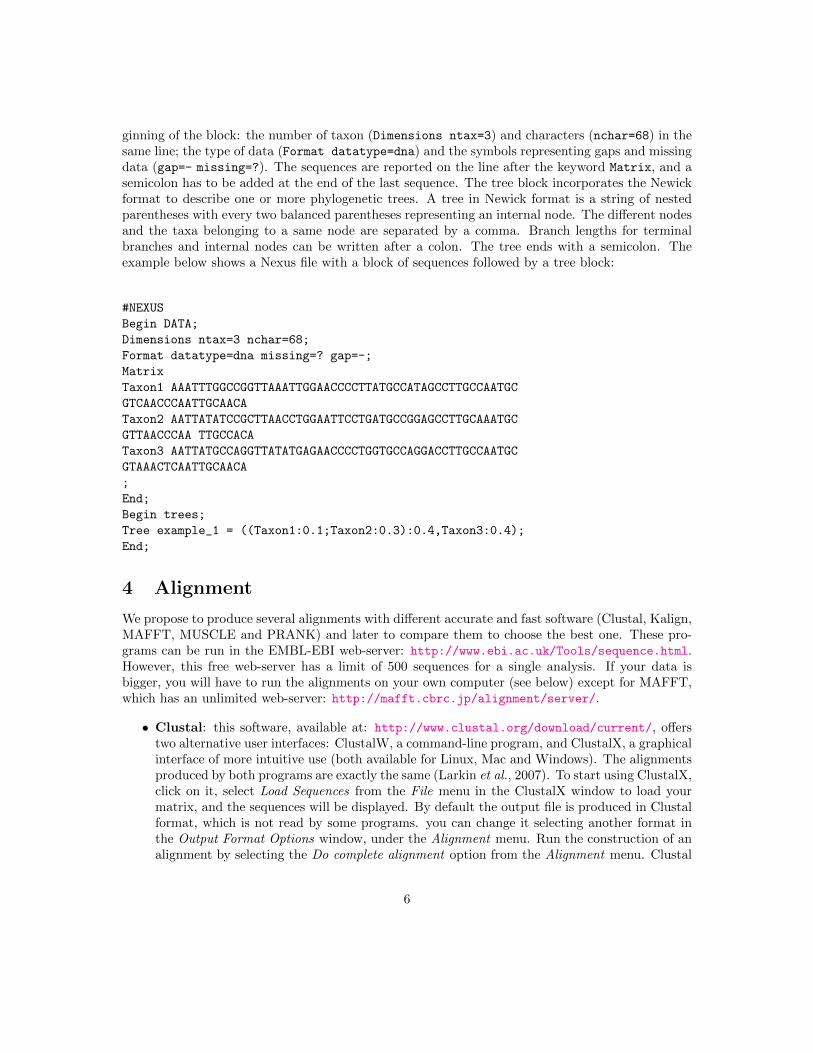
ginning of the block: the number of taxon (Dimensions ntax=3) and characters (nchar=68) in thesame line; the type of data (Format datatype=dna) and the symbols representing gaps and missingdata (gap=- missing=?). The sequences are reported on the line after the keyword Matrix, and asemicolon has to be added at the end of the last sequence. The tree block incorporates the Newickformat to describe one or more phylogenetic trees. A tree in Newick format is a string of nestedparentheses with every two balanced parentheses representing an internal node. The different nodesand the taxa belonging to a same node are separated by a comma. Branch lengths for terminalbranches and internal nodes can be written after a colon. The tree ends with a semicolon. Theexample below shows a Nexus file with a block of sequences followed by a tree block:

#NEXUS

Begin DATA;

Dimensions ntax=3 nchar=68;

Format datatype=dna missing=? gap=-;

Matrix

Taxon1 AAATTTGGCCGGTTAAATTGGAACCCCTTATGCCATAGCCTTGCCAATGC

GTCAACCCAATTGCAACA

Taxon2 AATTATATCCGCTTAACCTGGAATTCCTGATGCCGGAGCCTTGCAAATGC

GTTAACCCAA TTGCCACA

Taxon3 AATTATGCCAGGTTATATGAGAACCCCTGGTGCCAGGACCTTGCCAATGC

GTAAACTCAATTGCAACA

;

End;

Begin trees;

Tree example_1 = ((Taxon1:0.1;Taxon2:0.3):0.4,Taxon3:0.4);

End;

4 Alignment

We propose to produce several alignments with different accurate and fast software (Clustal, Kalign,MAFFT, MUSCLE and PRANK) and later to compare them to choose the best one. These pro-grams can be run in the EMBL-EBI web-server: http://www.ebi.ac.uk/Tools/sequence.html.However, this free web-server has a limit of 500 sequences for a single analysis. If your data isbigger, you will have to run the alignments on your own computer (see below) except for MAFFT,which has an unlimited web-server: http://mafft.cbrc.jp/alignment/server/.

• Clustal: this software, available at: http://www.clustal.org/download/current/, offerstwo alternative user interfaces: ClustalW, a command-line program, and ClustalX, a graphicalinterface of more intuitive use (both available for Linux, Mac and Windows). The alignmentsproduced by both programs are exactly the same (Larkin et al., 2007). To start using ClustalX,click on it, select Load Sequences from the File menu in the ClustalX window to load yourmatrix, and the sequences will be displayed. By default the output file is produced in Clustalformat, which is not read by some programs. you can change it selecting another format inthe Output Format Options window, under the Alignment menu. Run the construction of analignment by selecting the Do complete alignment option from the Alignment menu. Clustal

6

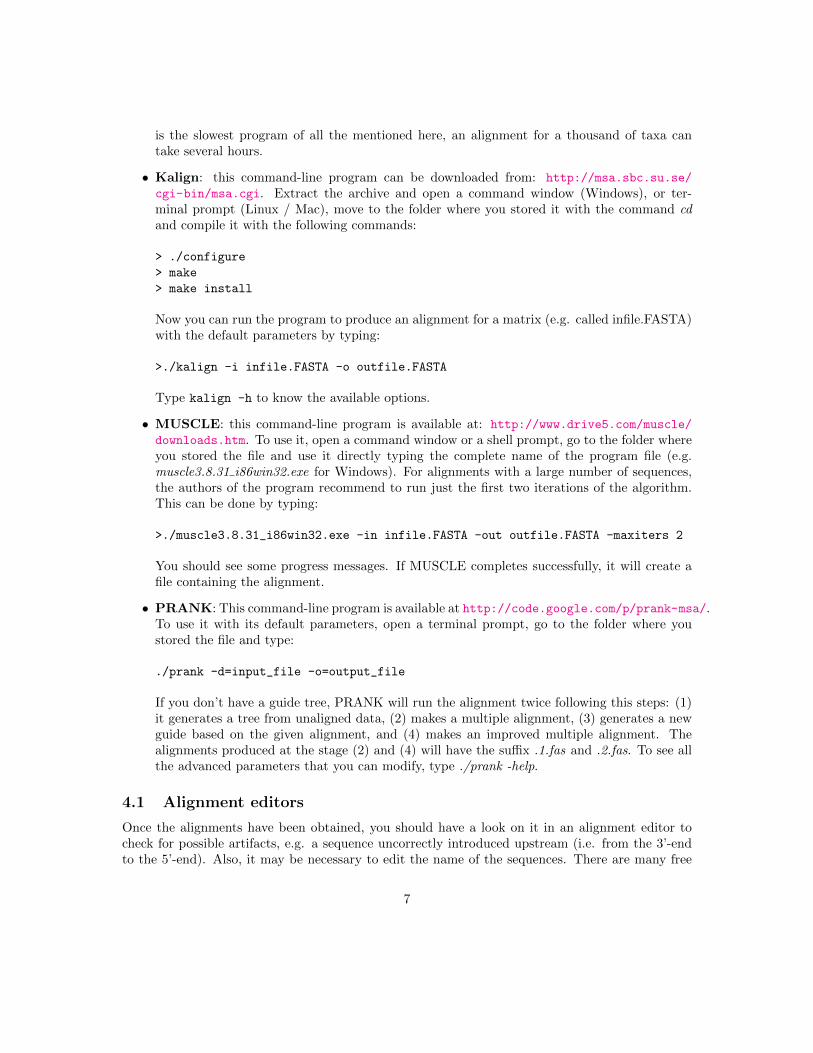
is the slowest program of all the mentioned here, an alignment for a thousand of taxa cantake several hours.

• Kalign: this command-line program can be downloaded from: http://msa.sbc.su.se/

cgi-bin/msa.cgi. Extract the archive and open a command window (Windows), or ter-minal prompt (Linux / Mac), move to the folder where you stored it with the command cdand compile it with the following commands:

> ./configure

> make

> make install

Now you can run the program to produce an alignment for a matrix (e.g. called infile.FASTA)with the default parameters by typing:

>./kalign -i infile.FASTA -o outfile.FASTA

Type kalign -h to know the available options.

• MUSCLE: this command-line program is available at: http://www.drive5.com/muscle/

downloads.htm. To use it, open a command window or a shell prompt, go to the folder whereyou stored the file and use it directly typing the complete name of the program file (e.g.muscle3.8.31 i86win32.exe for Windows). For alignments with a large number of sequences,the authors of the program recommend to run just the first two iterations of the algorithm.This can be done by typing:

>./muscle3.8.31_i86win32.exe -in infile.FASTA -out outfile.FASTA -maxiters 2

You should see some progress messages. If MUSCLE completes successfully, it will create afile containing the alignment.

• PRANK: This command-line program is available at http://code.google.com/p/prank-msa/.To use it with its default parameters, open a terminal prompt, go to the folder where youstored the file and type:

./prank -d=input_file -o=output_file

If you don’t have a guide tree, PRANK will run the alignment twice following this steps: (1)it generates a tree from unaligned data, (2) makes a multiple alignment, (3) generates a newguide based on the given alignment, and (4) makes an improved multiple alignment. Thealignments produced at the stage (2) and (4) will have the suffix .1.fas and .2.fas. To see allthe advanced parameters that you can modify, type ./prank -help.

4.1 Alignment editors

Once the alignments have been obtained, you should have a look on it in an alignment editor tocheck for possible artifacts, e.g. a sequence uncorrectly introduced upstream (i.e. from the 3’-endto the 5’-end). Also, it may be necessary to edit the name of the sequences. There are many free

7

programs for editing alignments that read most of the commonly used formats. To our opinion,the most complete and flexible one to date is BioEdit (available at: http://www.mbio.ncsu.

edu/BioEdit/bioedit.html, Hall, 1999), specially to obtain consensus sequences, but it is onlyavailable for Windows. Two more programs (good but less complete) to view and edit sequencesis Se-Al (Rambaut, 2002, http://tree.bio.ed.ac.uk/software/seal/) for Mac users, and Base-by-base (Brodie et al., 2004, http://athena.bioc.uvic.ca/tools/BaseByBase), available for allplatforms.

4.2 Choosing the best alignment for each region

Once the different alignments for one region have been obtained, MUMSA can be used to selectwhich is the best one, and to confirm that the sequences are not too divergent to be alignedtogether. It is available at the free web-server http://msa.sbc.su.se/cgi-bin/msa.cgi, whereyou just have to load the files of the different alignments and press Submit. Be aware that allalignments have to be in FASTA format and contain the sequences in the same order (sequencescan be sorted by name with an alignment editor). Once submitted, two scores will be displayedon the window’s browser: the average overlap score (AOS), and the multiple overlap score (MOS).The AOS score should be higher than 0.5; otherwise, the sequences are too divergent to be alignedconsistently, and in that case we recommend splitting the sequences in clusters going a step downin the taxonomic hierarchy, treating each cluster as a region in the final supermatrix, with missingdata for all the taxa that do not belong to the cluster. The alignment with the highest MOS is themost consistent one, and therefore the one that we will keep for the next step.

4.3 Alignment trimming

We suggest to trim the alignment selected for each region (i.e. to remove poorly aligned positions)with TrimAl, a program that automatically adjusts the parameters, based on the characteristicsof each alignment, to optimize the phylogenetic signal-to-noise ratio. TrimAl is a command-lineprogram available for the main operating systems (Linux, Mac, Windows). Download it from:http://trimal.cgenomics.org/downloads.

For Windows’ users, the program is already compiled in the bin directory. Linux and Mac usershave to compile the program. Open a terminal prompt and move to the directory containing thepackage’s source code and type make to compile it in the current directory. Suppose you have analignment called infile.fasta and you want to obtain a file (outfile.fasta) with the trimmed alignment.Drop the alignment file in the bin directory and type in the command line (substitute trimal bytrimal.exe if you are using Windows):

> trimal -in infile.FASTA -out outfile.FASTA -automated1

The option -automated1 will remove columns from the input alignment using the heuristicautomated1 method to decide which is the best method to trim the alignment between gappyoutand strict ones. The output file will be created in the bin directory.

4.4 Concatenating regions in a single supermatrix

We propose two options to concatenate different alignment matrices in a single supermatrix:

8

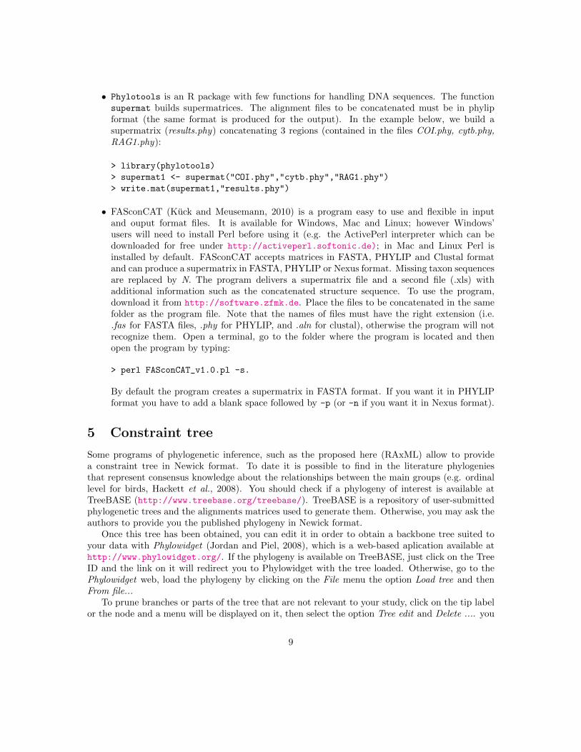
• Phylotools is an R package with few functions for handling DNA sequences. The functionsupermat builds supermatrices. The alignment files to be concatenated must be in phylipformat (the same format is produced for the output). In the example below, we build asupermatrix (results.phy) concatenating 3 regions (contained in the files COI.phy, cytb.phy,RAG1.phy):

> library(phylotools)

> supermat1 <- supermat("COI.phy","cytb.phy","RAG1.phy")

> write.mat(supermat1,"results.phy")

• FASconCAT (Kuck and Meusemann, 2010) is a program easy to use and flexible in inputand ouput format files. It is available for Windows, Mac and Linux; however Windows’users will need to install Perl before using it (e.g. the ActivePerl interpreter which can bedownloaded for free under http://activeperl.softonic.de); in Mac and Linux Perl isinstalled by default. FASconCAT accepts matrices in FASTA, PHYLIP and Clustal formatand can produce a supermatrix in FASTA, PHYLIP or Nexus format. Missing taxon sequencesare replaced by N. The program delivers a supermatrix file and a second file (.xls) withadditional information such as the concatenated structure sequence. To use the program,download it from http://software.zfmk.de. Place the files to be concatenated in the samefolder as the program file. Note that the names of files must have the right extension (i.e..fas for FASTA files, .phy for PHYLIP, and .aln for clustal), otherwise the program will notrecognize them. Open a terminal, go to the folder where the program is located and thenopen the program by typing:

> perl FASconCAT_v1.0.pl -s.

By default the program creates a supermatrix in FASTA format. If you want it in PHYLIPformat you have to add a blank space followed by -p (or -n if you want it in Nexus format).

5 Constraint tree

Some programs of phylogenetic inference, such as the proposed here (RAxML) allow to providea constraint tree in Newick format. To date it is possible to find in the literature phylogeniesthat represent consensus knowledge about the relationships between the main groups (e.g. ordinallevel for birds, Hackett et al., 2008). You should check if a phylogeny of interest is available atTreeBASE (http://www.treebase.org/treebase/). TreeBASE is a repository of user-submittedphylogenetic trees and the alignments matrices used to generate them. Otherwise, you may ask theauthors to provide you the published phylogeny in Newick format.

Once this tree has been obtained, you can edit it in order to obtain a backbone tree suited toyour data with Phylowidget (Jordan and Piel, 2008), which is a web-based aplication available athttp://www.phylowidget.org/. If the phylogeny is available on TreeBASE, just click on the TreeID and the link on it will redirect you to Phylowidget with the tree loaded. Otherwise, go to thePhylowidget web, load the phylogeny by clicking on the File menu the option Load tree and thenFrom file...

To prune branches or parts of the tree that are not relevant to your study, click on the tip labelor the node and a menu will be displayed on it, then select the option Tree edit and Delete .... you

9

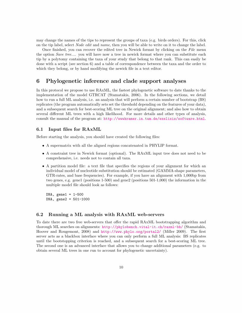
may change the names of the tips to represent the groups of taxa (e.g. birds orders). For this, clickon the tip label, select Node edit and name, then you will be able to write on it to change the label.

Once finished, you can recover the edited tree in Newick format by clicking on the File menuthe option Save tree.... you will have now a tree in newick format where you can substitute eachtip by a polytomy containing the taxa of your study that belong to that rank. This can easily bedone with a script (see section 6) and a table of correspondence between the taxa and the order towhich they belong, or by hand modifying the newick file in a text editor.

6 Phylogenetic inference and clade support analyses

In this protocol we propose to use RAxML, the fastest phylogenetic software to date thanks to theimplementation of the model GTRCAT (Stamatakis, 2006). In the following sections, we detailhow to run a full ML analysis, i.e. an analysis that will perform a certain number of bootstrap (BS)replicates (the program automatically sets set the threshold depending on the features of your data),and a subsequent search for best-scoring ML tree on the original alignment; and also how to obtainseveral different ML trees with a high likelihood. For more details and other types of analysis,consult the manual of the program at: http://wwwkramer.in.tum.de/exelixis/software.html.

6.1 Input files for RAxML

Before starting the analysis, you should have created the following files:

• A supermatrix with all the aligned regions concatenated in PHYLIP format.

• A constraint tree in Newick format (optional). The RAxML input tree does not need to becomprehensive, i.e. needs not to contain all taxa.

• A partition model file: a text file that specifies the regions of your alignment for which anindividual model of nucleotide substitution should be estimated (GAMMA-shape parameters,GTR-rates, and base frequencies). For example, if you have an alignment with 1,000bp fromtwo genes, e.g. gene1 (positions 1-500) and gene2 (positions 501-1,000) the information in themultiple model file should look as follows:

DNA, gene1 = 1-500

DNA, gene2 = 501-1000

6.2 Running a ML analysis with RAxML web-servers

To date there are two free web-servers that offer the rapid RAxML bootstrapping algorithm andthorough ML searches on alignments: http://phylobench.vital-it.ch/raxml-bb/ (Stamatakis,Hoover and Rougemont, 2008) and http://www.phylo.org/portal2/ (Miller 2009). The firstserver acts as a blackbox interface where you can only perform a full ML analysis: BS replicatesuntil the bootstopping criterion is reached, and a subsequent search for a best-scoring ML tree.The second one is an advanced interface that allows you to change additional parameters (e.g. toobtain several ML trees in one run to account for phylogenetic uncertainty).

10

6.2.1 Blackbox interface server

To run your analysis in the http://phylobench.vital-it.ch/raxml-bb/web-server, go to thiswebpage, load the supermatrix in PHYLIP format, the constraint tree in Newick format (if avail-able), and the partitioned model file; write the names of the outgroup, and check the option Maxi-mum likelihood search before clicking the Run button. A full analysis (BS replicates and search fora best-scoring ML tree) will be done. Once the job is finished, you will receive a mail with a linkto a webpage where you can download the output files.

6.2.2 Advanced interface server

If you run your analysis in http://www.phylo.org/portal2/ you will have to create first a useraccount, and then create a folder where you will host the data and tasks. Click on Create newfolder, give it a name (label). Now, go to the menu on the left side and click on Data and then toEnter data, to upload all the input files required for a RAxML analysis and click on Save. Click onTasks in your folder menu to run a job: click on create a new task, load the required files by clickingon select input data and then on select tool, choose the program RAxML-HPC2 on Abe (7.2.6), andclick on parameters to adjust the settings for the run. There are 34 parameters, most of them havea default setting that works well. However you should at least adjust the following ones:

• Maximum Hours to Run: change it to 168 (the maximum) if your are handling big data,otherwise the run may be killed before it ends.

• Number of chars in your dataset : write the number of base pairs of your alignment for onetaxa.

• Outgroup: indicate the name of the outgroups, separating them with a comma.

• Constraint : select the file containing your constraint tree.

• Use a mixed/partitioned model : If you want RAxML to estimate the model parameters foreach region, load the partition model file here.

Then, if you click on Save parameters and Submit, the web-server will do a typical full ML analysis(BS replicates and search for a best-scoring ML tree). To obtain more than one single best MLtree, go to the Advanced parameters section, uncheck the option Conduct rapid bootstraping andthen check Specify the number alternative runs on distinct starting trees and write the number ofML trees you want to obtain in Enter the number of alternative runs. Once the job is finished, youwill receive a mail with a link to your user account, where you can download the output files (seeOutput files section below) going to the Tasks folder, clicking on View Output.

6.3 Running a ML analysis with RAxML in a personal computer

You may need to run the RAxML analysis on your personal computer; e.g. if your data is really hugeit may take more than 7 days (which is the current limit time for the web-servers). The programis available at: http://wwwkramer.in.tum.de/exelixis/software.html. Below we detail how toinstall and run an analysis with RAxML directly, but you can also call RAxML from R with thephyloch package, available at: http://www.christophheibl.de/Rpackages.html.

11

• Installing and compiling RAxML for Linux and Mac users: Open a terminal prompt, go to thedirectory containing the downloaded file, type bunzip2 RAxML-7.2.6.tar.bz2 (if it does notwork write the full path for the downloaded file) and then tar xf RAxML-7.2.6.tar. Thiswill create a directory called RAxML-7.2.6. Move to this directory. Compile the RAxMLexecutable for the standard sequential version by typing: make -f Makefile.gcc. This willgenerate an executable called raxmlHPC. If you have a multi-core computer, you may prefer tocompile the Pthreads-parallelized version of RAxML (raxmlHPC-PTHREADS). To compileit, type -f Makefile.PTHREADS or make -f Makefile.PTHREADS.MAC on Mac.

• Installing RAxML for Windows’ users: Unzip the file raxml-win32-100315.tar.gz. To runthe program, you just have to open a command window and go to the directory where youallocated the extracted files (raxmlHPC.exe and raxmlHPC-PTHREADS.exe), and write thename of the version of the program preferred (raxmlHPC.exe is the sequential version, whileraxmlHPC-PTHREADS.exe is the Pthreads-parallelized version for multi-core computers)followed by the necessary commands (see next section).

• Running a full ML analysis (bootstrapping and search for the best-scoring ML tree): Firstof all, place the input files in the same folder where the executable file of raxml is allocated.Open a command window (or a shell prompt), go to the directory containing the programand the input files. Then you should type:

>./raxmlHPC -s infile.phy -n result -g multiConstraint.txt

-q DNApartition.txt -o outgroup -f a -m GTRCAT -x 12345 -#100

where infile.phy is the name of the concatenated alignment in PHYLIP format, result is thename that the program will give to the output, multiConstraint.txt is a file containing aconstraint tree written in Newick format, DNApartition.txt is a text file where you specifythe first and last position of each region included in your analysis, outgroup is the namethat your choosen outgroup has in the matrix. To allow RAxML automatically determine asufficient number of BS replicates, replace -# 100 by one of the BS convergence criteria: -#autoFC, -# autoMRE, -# autoMR, -# autoMRE IGN (for more information on the differentcriteria, see Pattengale et al. 2010). If you do not have one of the inputs (e.g. a constrainttree), eliminate the flag before the name of the file (in that case, you would not write -g

multiConstraint.txt). Note that if you are using the P-Threads version of RAxML formulti-core computers you should write raxmlHPC-PTHREADS instead of raxmlHPC, and makesure to specify the exact number of CPUs available on your system with the -T flag, e.g. ifyou have 4 cores, your command line should start as raxmlHPC-PTHREADS -T 4. If you useWindows add .exe at the end of the name of the program.

• Obtaining several ML trees: To obtain several ML trees in a single run, specify a number ofalternative runs on distinct starting trees with the flag -N. For example, if -f d -N 100 isspecified, RAxML will compute 100 distinct ML trees starting from 100 distinct randomizedmaximum parsimony starting trees with the rapid hill climbing algorithm (Stamatakis et al.2008). To set this, type:

> ./raxmlHPC -f d -N 100 -g multiConstraint.txt -m GTRMIX

-q DNApartition.txt -s infile.phy -o outgroup

12

• Computing clade support by means of rapid bootstrapping analysis: To set e.g. a BS analysisof 100 replicates with a random seed number (e.g. 12345), type:

> ./raxmlHPC -x 12345 -g multiConstraint.txt -m GTRGAMMA

-q DNApartition.txt -s infile.phy -# 100 -o outgroup

To allow RAxML automatically determine a sufficient number of BS replicates, replace -#100 by one of the BS convergence criteria: -# autoFC, -# autoMRE, -# autoMR or -#autoMRE IGN.

6.4 Output files

After running a full ML analysis, the following output files will be produced:

• a single file with the bootstrapped trees in Newick format (called raxml bootstrap.result)

• the consensus tree of the BS trees in Newick (outtree)

• the best-scoring ML tree with branch lengths corresponding to the number of substitutionsper branch estimated (raxml bestTree.result)

• the best-scoring ML tree with branch lengths and BS support values (raxml bipartitions.result)

• a text with the job report (raxml info.result), which contains information about the modelparameters inferred, algorithm used and how RAxML was called, and the final likelihood

If you run an analysis to obtain several ML trees, you will obtain one file for each ML treeproduced, with the ending .run followed by a number.

7 Estimation of divergence times

To convert phylograms (i.e. branch lengths proportional to evolutionary change) into chronograms(i.e. branch lenghts indicating time), several methods exist. We explain here how to use two meth-ods: the Penalized-Likelihood approach with r8s (Sanderson, 2003), which it is computationally lessdemanding than bayesian methods; and the Mean Path Lengths method implemented in PATHd8(Britton et al., 2007), which can date huge trees in a very short time. For those interested in thebayesian method implemented in Multidivtime, a detailed step-by-step manual has been writtenby Rutschmann (2005), and a implementation in R of this approach (Lagopus) has been developedby Heibl and Cusimano (2008), available at: http://www.christophheibl.de/mdt/mdtinr.html.

7.1 Penalized-likelihood with r8s

To estimate divergence times with r8s, you need a tree with branch-lengths and fossil calibrationsor constraints to convert relative to absolute ages. The procedure is composed of two steps: across-validation analysis to find the best smoothing value and a divergence analysis in which the

13

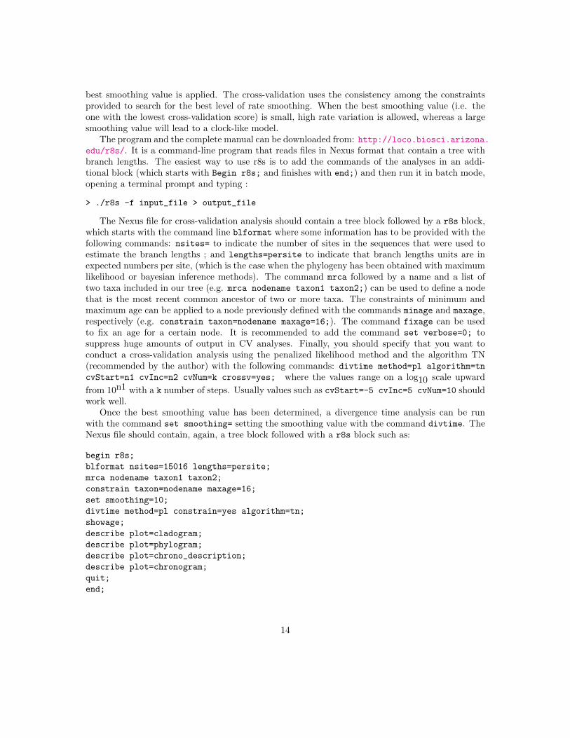
best smoothing value is applied. The cross-validation uses the consistency among the constraintsprovided to search for the best level of rate smoothing. When the best smoothing value (i.e. theone with the lowest cross-validation score) is small, high rate variation is allowed, whereas a largesmoothing value will lead to a clock-like model.

The program and the complete manual can be downloaded from: http://loco.biosci.arizona.edu/r8s/. It is a command-line program that reads files in Nexus format that contain a tree withbranch lengths. The easiest way to use r8s is to add the commands of the analyses in an addi-tional block (which starts with Begin r8s; and finishes with end;) and then run it in batch mode,opening a terminal prompt and typing :

> ./r8s -f input_file > output_file

The Nexus file for cross-validation analysis should contain a tree block followed by a r8s block,which starts with the command line blformat where some information has to be provided with thefollowing commands: nsites= to indicate the number of sites in the sequences that were used toestimate the branch lengths ; and lengths=persite to indicate that branch lengths units are inexpected numbers per site, (which is the case when the phylogeny has been obtained with maximumlikelihood or bayesian inference methods). The command mrca followed by a name and a list oftwo taxa included in our tree (e.g. mrca nodename taxon1 taxon2;) can be used to define a nodethat is the most recent common ancestor of two or more taxa. The constraints of minimum andmaximum age can be applied to a node previously defined with the commands minage and maxage,respectively (e.g. constrain taxon=nodename maxage=16;). The command fixage can be usedto fix an age for a certain node. It is recommended to add the command set verbose=0; tosuppress huge amounts of output in CV analyses. Finally, you should specify that you want toconduct a cross-validation analysis using the penalized likelihood method and the algorithm TN(recommended by the author) with the following commands: divtime method=pl algorithm=tn

cvStart=n1 cvInc=n2 cvNum=k crossv=yes; where the values range on a log10 scale upward

from 10n1 with a k number of steps. Usually values such as cvStart=-5 cvInc=5 cvNum=10 shouldwork well.

Once the best smoothing value has been determined, a divergence time analysis can be runwith the command set smoothing= setting the smoothing value with the command divtime. TheNexus file should contain, again, a tree block followed with a r8s block such as:

begin r8s;

blformat nsites=15016 lengths=persite;

mrca nodename taxon1 taxon2;

constrain taxon=nodename maxage=16;

set smoothing=10;

divtime method=pl constrain=yes algorithm=tn;

showage;

describe plot=cladogram;

describe plot=phylogram;

describe plot=chrono_description;

describe plot=chronogram;

quit;

end;

14

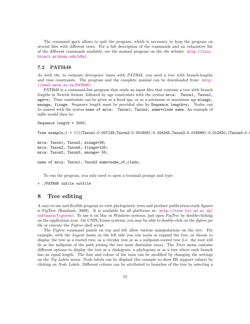
The command quit allows to quit the program, which is necessary to loop the program onseveral files with different trees. For a full description of the commands and an exhaustive listof the different commands available, see the manual program on the r8s website: http://loco.

biosci.arizona.edu/r8s/.

7.2 PATHd8

As with r8s, to estimate divergence times with PATHd8, you need a tree with branch-lengthsand time constraints. The program and the complete manual can be downloaded from: http:

//www2.math.su.se/PATHd8/.PATHd8 is a command-line program that reads an input files that contains a tree with branch

lengths in Newick format, followed by age constraints with the syntax mrca: Taxon1, Taxon2,

age=x;. Time constraints can be given as a fixed age, or as a minimum or maximum age minage,

maxage, fixage. Sequence length must be provided also by Sequence length=x;. Nodes canbe named with the syntax name of mrca: Taxon1, Taxon2, name=clade name. An example ofinfile would then be:

Sequence length = 2000;

Tree example_1 = ((((Taxon1:0.007148,Taxon2:0.001808):0.024345,Taxon3:0.016588):0.012920,(Taxon4:0.018119,Taxon5:0.006232):0.004708):0.028037,Taxon6:0.005244);

mrca: Taxon1, Taxon2, minage=26;

mrca: Taxon2, Taxon6, fixage=125;

mrca: Taxon2, Taxon3, maxage= 55;

name of mrca: Taxon1, Taxon2 name=name_of_clade;

To run the program, you only need to open a terminal prompt and type:

> ./PATHd8 infile outfile

8 Tree editing

A easy-to-use and flexible program to view phylogenetic trees and produce publication-ready figuresis FigTree (Rambaut, 2009). It is available for all platforms at: http://tree.bio.ed.ac.uk/

software/figtree/. To use it on Mac or Windows systems, just open FigTree by double-clickingon the application icon. On UNIX/Linux systems, you may be able to double-click on the figtree.jarfile or execute the Figtree shell script.

The Figtree command panels on top and left allow various manipulations on the tree. Forexample, with the Layout menu on the left side you can zoom or expand the tree, or choose todisplay the tree as a rooted tree, as a circular tree or as a midpoint-rooted tree (i.e. the root willlie at the midpoint of the path joining the two most dissimilar taxa). The Trees menu containsdifferent options to display the tree as a cladogram, a phylogram or as a tree where each branchhas an equal length. The font and colour of the taxa can be modified by changing the settingson the Tip Labels menu. Node labels can be displaid (for example to show BS support values) byclicking on Node Labels. Different colours can be attributed to branches of the tree by selecting a

15

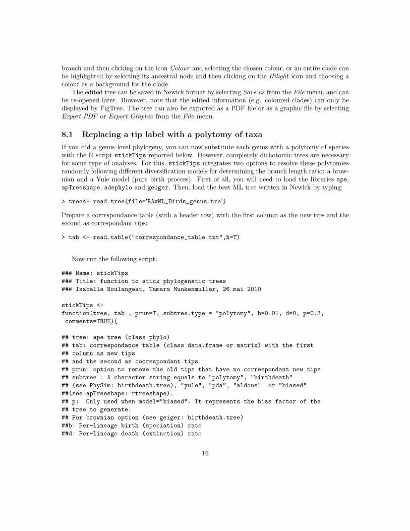
branch and then clicking on the icon Colour and selecting the chosen colour, or an entire clade canbe highlighted by selecting its ancestral node and then clicking on the Hilight icon and choosing acolour as a background for the clade.

The edited tree can be saved in Newick format by selecting Save as from the File menu, and canbe re-opened later. However, note that the edited information (e.g. coloured clades) can only bedisplayed by FigTree. The tree can also be exported as a PDF file or as a graphic file by selectingExport PDF or Export Graphic from the File menu.

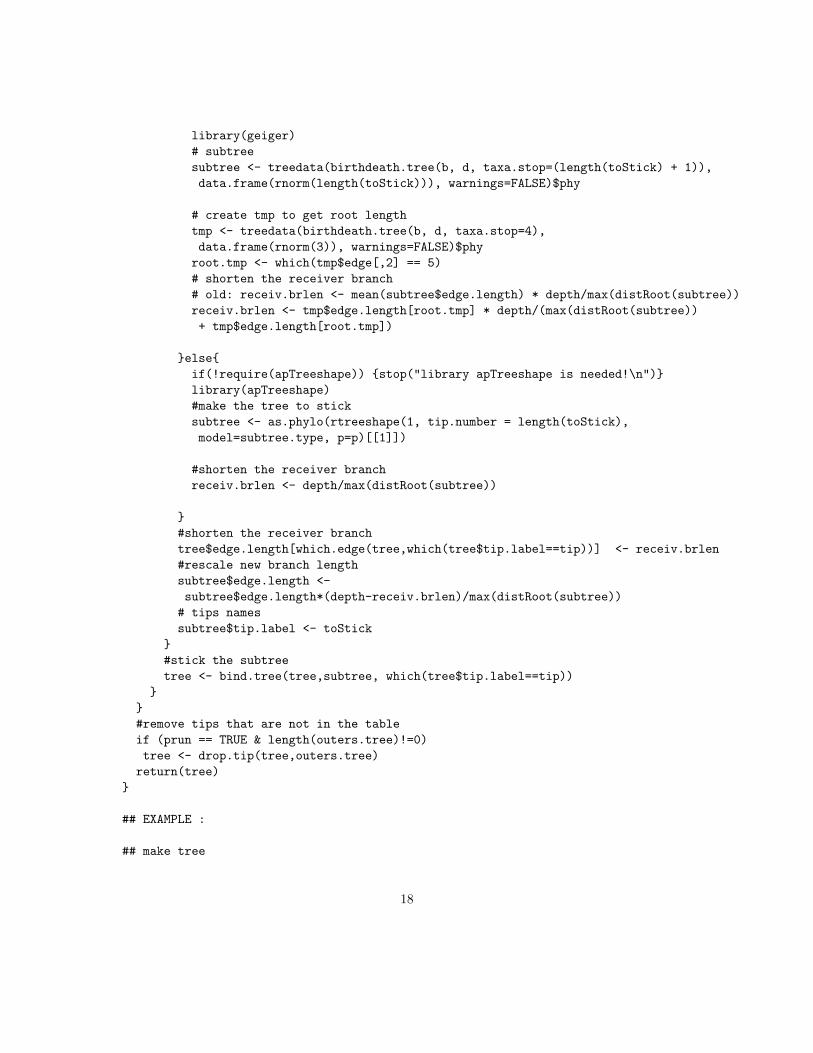
8.1 Replacing a tip label with a polytomy of taxa

If you did a genus level phylogeny, you can now substitute each genus with a polytomy of specieswith the R script stickTips reported below. However, completely dichotomic trees are necessaryfor some type of analyses. For this, stickTips integrates two options to resolve these polytomiesrandomly following different diversification models for determining the branch length ratio: a brow-nian and a Yule model (pure birth process). First of all, you will need to load the libraries ape,apTreeshape, adephylo and geiger. Then, load the best ML tree written in Newick by typing:

> tree<- read.tree(file='RAxML_Birds_genus.tre')

Prepare a correspondance table (with a header row) with the first column as the new tips and thesecond as correspondant tips:

> tab <- read.table("correspondance_table.txt",h=T)

Now run the following script:

### Name: stickTips

### Title: function to stick phylogenetic trees

### Isabelle Boulangeat, Tamara Munkenmuller, 26 mai 2010

stickTips <-

function(tree, tab , prun=T, subtree.type = "polytomy", b=0.01, d=0, p=0.3,

comments=TRUE){

## tree: ape tree (class phylo)

## tab: correspondance table (class data.frame or matrix) with the first

## column as new tips

## and the second as coorespondant tips.

## prun: option to remove the old tips that have no correspondant new tips

## subtree : A character string equals to "polytomy", "birthdeath"

## (see PhySim: birthdeath.tree), "yule", "pda", "aldous" or "biased"

##(see apTreeshape: rtreeshape).

## p: Only used when model="biased". It represents the bias factor of the

## tree to generate.

## For brownian option (see geiger: birthdeath.tree)

##b: Per-lineage birth (speciation) rate

##d: Per-lineage death (extinction) rate

16

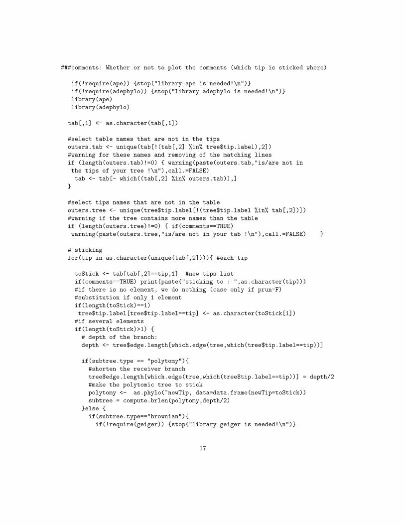
###comments: Whether or not to plot the comments (which tip is sticked where)

if(!require(ape)) {stop("library ape is needed!\n")}

if(!require(adephylo)) {stop("library adephylo is needed!\n")}

library(ape)

library(adephylo)

tab[,1] <- as.character(tab[,1])

#select table names that are not in the tips

outers.tab <- unique(tab[!(tab[,2] %in% tree$tip.label),2])

#warning for these names and removing of the matching lines

if (length(outers.tab)!=0) { warning(paste(outers.tab,"is/are not in

the tips of your tree !\n"),call.=FALSE)

tab <- tab[- which((tab[,2] %in% outers.tab)),]

}

#select tips names that are not in the table

outers.tree <- unique(tree$tip.label[!(tree$tip.label %in% tab[,2])])

#warning if the tree contains more names than the table

if (length(outers.tree)!=0) { if(comments==TRUE)

warning(paste(outers.tree,"is/are not in your tab !\n"),call.=FALSE) }

# sticking

for(tip in as.character(unique(tab[,2]))){ #each tip

toStick <- tab[tab[,2]==tip,1] #new tips list

if(comments==TRUE) print(paste("sticking to : ",as.character(tip)))

#if there is no element, we do nothing (case only if prun=F)

#substitution if only 1 element

if(length(toStick)==1)

tree$tip.label[tree$tip.label==tip] <- as.character(toStick[1])

#if several elements

if(length(toStick)>1) {

# depth of the branch:

depth <- tree$edge.length[which.edge(tree,which(tree$tip.label==tip))]

if(subtree.type == "polytomy"){

#shorten the receiver branch

tree$edge.length[which.edge(tree,which(tree$tip.label==tip))] = depth/2

#make the polytomic tree to stick

polytomy <- as.phylo(~newTip, data=data.frame(newTip=toStick))

subtree = compute.brlen(polytomy,depth/2)

}else {

if(subtree.type=="brownian"){

if(!require(geiger)) {stop("library geiger is needed!\n")}

17

library(geiger)

# subtree

subtree <- treedata(birthdeath.tree(b, d, taxa.stop=(length(toStick) + 1)),

data.frame(rnorm(length(toStick))), warnings=FALSE)$phy

# create tmp to get root length

tmp <- treedata(birthdeath.tree(b, d, taxa.stop=4),

data.frame(rnorm(3)), warnings=FALSE)$phy

root.tmp <- which(tmp$edge[,2] == 5)

# shorten the receiver branch

# old: receiv.brlen <- mean(subtree$edge.length) * depth/max(distRoot(subtree))

receiv.brlen <- tmp$edge.length[root.tmp] * depth/(max(distRoot(subtree))

+ tmp$edge.length[root.tmp])

}else{

if(!require(apTreeshape)) {stop("library apTreeshape is needed!\n")}

library(apTreeshape)

#make the tree to stick

subtree <- as.phylo(rtreeshape(1, tip.number = length(toStick),

model=subtree.type, p=p)[[1]])

#shorten the receiver branch

receiv.brlen <- depth/max(distRoot(subtree))

}

#shorten the receiver branch

tree$edge.length[which.edge(tree,which(tree$tip.label==tip))] <- receiv.brlen

#rescale new branch length

subtree$edge.length <-

subtree$edge.length*(depth-receiv.brlen)/max(distRoot(subtree))

# tips names

subtree$tip.label <- toStick

}

#stick the subtree

tree <- bind.tree(tree,subtree, which(tree$tip.label==tip))

}

}

#remove tips that are not in the table

if (prun == TRUE & length(outers.tree)!=0)

tree <- drop.tip(tree,outers.tree)

return(tree)

}

## EXAMPLE :

## make tree

18

#tre <- rtree(10)

#tre <- compute.brlen(chronogram(tre))

#tre$tip.label <- paste("genus",1:10, sep="")

#plot(tre)

#

## make correspondance table

#

#ctab <- data.frame(species = paste("sp",1:50,sep=""),

#Genus = sample(tre$tip.label[-1], 50, replace=T))

#

## stick tips

#

#par(mfrow=c(1,3))

#tre2 <- stickTips(tre, ctab, prun=F)

#plot(tre2) ; title("polytomy")

#tre3 <- stickTips(tre, ctab, prun=F, subtree.type="yule")

#plot(tre3) ; title("yule")

#tre4 <- stickTips(tre, ctab, prun=F, subtree.type="brownian")

#plot(tre4) ; title("brownian")

#

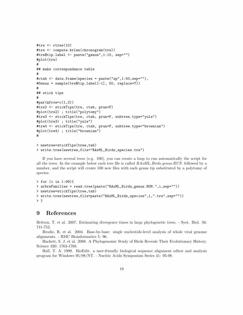
> newtree=stickTips(tree,tab)

> write.tree(newtree,file="RAxML_Birds_species.tre")

If you have several trees (e.g. 100), you can create a loop to run automatically the script forall the trees. In the example below each tree file is called RAxML Birds genus.RUN. followed by anumber, and the script will create 100 new files with each genus tip substituted by a polytomy ofspecies:

> for (i in 1:99){

> arbreFamilles = read.tree(paste("RAxML_Birds_genus.RUN.",i,sep=""))

> newtree=stickTips(tree,tab)

> write.tree(newtree,file=paste("RAxML_Birds_species",i,".tre",sep=""))

> }

9 References

Britton, T. et al. 2007. Estimating divergence times in large phylogenetic trees. - Syst. Biol. 56:741-752.

Brodie, R. et al. 2004. Base-by-base: single nucleotide-level analysis of whole viral genomealignments. - BMC Bioinformatics 5: 96.

Hackett, S. J. et al. 2008. A Phylogenomic Study of Birds Reveals Their Evolutionary History.Science 320: 1763-1768.

Hall, T. A. 1999. BioEdit: a user-friendly biological sequence alignment editor and analysisprogram for Windows 95/98/NT. - Nucleic Acids Symposium Series 41: 95-98.

19

Heibl, C. and Cusimano, N. 2008. LAGOPUS - Divergence time estimation in R using themultidivtime approach.

Jordan, G. E. and Piel, W. H. 2008. PhyloWidget: web-based visualizations for the tree of life.- Bioinformatics 24: 1641-1642.

Kuck, P. and Meusemann, K. 2010. FASconCAT: Convenient handling of data matrices. -Molecular Phylogenetics and Evolution 56: 1115-1118.

Larkin, M. A. et al. 2007. Clustal W and Clustal X version 2.0. - Bioinformatics 23: 2947-2948.Lemey, P. et al. 2010. The phylogenetic handbook. A practical approach to phylogenetic

analysis and hypothesis testing. - Cambridge University Press.Maddison, D. R. et al. 1997. NEXUS: An Extensible file format for Systematic Information. -

Systematic Biology 46: 590-621.Miller, M. A. et al. 2009. The CIPRES Portals. http://www.phylo.org/sub_sections/

portal.Paradis, E. 2006. Analysis of Phylogenetics and Evolution with R. - Springer-Verlag.Pattengale, N. et al. 2010. How many bootstrap replicates are necessary? - J. Comp. Biol 17:

337-354.Rambaut, A. 2002. Se-Al v.2.0.http://evolve.zoo.ox.ac.uk/software/Rambaut, A. 2009. FigTree v1.3.1. http://tree.bio.ed.ac.uk/software/figtree/Sanderson, M. J. 2003. r8s: inferring absolute rates of molecular evolution and divergence times

in the absence of a molecular clock. - Bioinformatics 19: 301-302.Stamatakis, A. 2006. RAxML-VI-HPC: maximum likelihood-based phylogenetic analyses with

thousands of taxa and mixed models. - Bioinformatics 22: 2688-2690.Stamatakis, A. et al. 2008. A Rapid Bootstrap Algorithm for the RAxML Web-Servers. Sys-

tematic Biology 75: 758-771.Thuiller, W. et al. 2011. Consequences of climate change on the Tree of Life in Europe. Nature

470: 531-534.

20