Download: SimpleMaxentPLact.xlsx SimpleMaxentPPunct.xlsx SimpleMaxentTableE1.xlsx

Ecography E7872Merow, C., Smith, M. J. and Silander, Jr J. A. 2013. A practical guide to MaxEnt for modeling species’ distributions: what it does, and why inputs and settings matter. – Ecography 36: xxx–xxx.

Supplementary material

  

42 

Appendix 1: Glossary

Background sample: A sample from the landscape of locations that are considered to be a priori

equally likely to contain individuals. Presence/absence is unknown at these locations. MaxEnt

contrasts the features at the occupied locations to those in the background sample.

Biased background method: A biased background uses a uniform prior but modifies the selection of

background points to have the same sampling bias as the presences. This is often done with target

group sampling.

Biased prior method: Using a biased prior gives a nonuniform weighting to a given set of

background points to account for sampling bias. The user provides an estimate of the relative

search effort in each location on the landscape, which is used as the prior (Q(z(xi)). The biased

prior has the same multinomial probabilistic interpretation as the predictions in geographic space

and reflects the assumption that the relative probability of observing an individual in a given

location is based on the search effort there.

Clamping: When projecting models fit on one landscape onto another landscape, the new landscape

may encompass environmental conditions beyond the range of the conditions observed in the

fitting landscape. In this case, the response curve may be clamped beyond the range of the fitting

data by setting it at a constant value equal to the predicted value at the range edge.

Entropy: A measure of uncertainty. In the context of the MaxEnt software package, one maximizes

the uncertainty (entropy) of the predicted distribution in order to obtain the most conservative

estimate possible, given the data. Therefore, the predicted contains as little information as possible

about which cell is most likely to contain an individual, which corresponds to a prediction that is as

uniform as possible in geographic space.

  

43 

Environmental space: MaxEnt models can be described in terms of the probability densities of

environmental covariates (Elith et al. 2011). This formulation is helpful for thinking about how the

data are used to build response curves (Figs. 1, 3). This contrasts with the geographic space

formulation, wherein the model is described in terms of a probability density over the landscape.

Feature: A mathematical function of an environmental predictor. Each environmental predictor can

generate multiple features; linear, quadratic, product, threshold and hinge features can be

constructed from a single environmental predictor.

Feature Classes: A functional form of an environmental predictor.

Linear – These constrain the mean of environmental predictors.

Quadratic – These constrain the variance of environmental predictors when linear features are also

used.

Product – Interaction terms for pairwise combinations of environmental predictors. These constrain

the covariance of environmental predictors when linear features are also used.

Threshold – A step function. One is produced between each successive pair of data points.

Hinge – Like a threshold feature, but linear above the threshold value. Hinges are piecewise

combinations of a line with slope zero and one with slope nonzero. These should not be used

with linear features as linear features are a special case of hinge features. Forward hinges have

the constant piece to the left of the linear piece and reverse hinges have the constant piece to

the right of the linear piece.

  

44 

Threshold Functions Forward Hinge Functions Reverse Hinge Functions

Gain: The penalized likelihood function maximized by MaxEnt. Exponentiating the gain gives the

likelihood ratio of an average presence to an average background point.

Geographic space: MaxEnt models can be described in terms of a multinomial probability density

over cells of a landscape. This formulation is helpful for thinking about prior distributions,

particularly related to sampling bias. This contrasts with the environmental space formulation,

wherein the model is described in terms of probability densities of environmental covariates (Elith

et al. 2011).

k-fold cross validation: K-fold cross validation splits the data into k independent subsets, and for each

subset, trains the model with k-1 subsets and evaluates the model on the kth subset.

Mask: A term for a GIS layer used to withhold certain locations on the landscape from an analysis. A

mask is fake predictor with a value of 1 (or any constant) at locations to be included in the analysis

and NA at locations to be excluded. This can be useful for constrain how background points are

selected.

Multinomial distribution: A multinomial distribution is a generalization of a binomial distribution,

where more than two categories are possible. There are a finite number of localities (xi) in the

landscape and each locality represents a different category in the multinomial distribution. MaxEnt

  

45 

assigns a probability to each locality and rescales them such that all the probabilities across the

landscape sum to unity.

Normalization: The process to ensure that MaxEnt’s predicted RORs (raw output) sum to one. This

ensures that MaxEnt’s prediction is a proper multinomial distribution in geographic space.

Normalization is performed by dividing the predicted probability in a cell by the sum of predicted

probabilities across the landscape; this is done automatically by MaxEnt over the training data set

(but not when projecting models).

Occurrence rate: A prediction of the abundance of a species in a cell (i.e. the rate parameter of a

Poisson distribution).

Relative Occurrence Rate (ROR): The occurrence rate, normalized to sum to unity over the

landscape. Given that an individual was observed, the ROR is interpreted as the relative probability

that the sample derived from each cell on the landscape. In other words, the ROR is the relative

probability that a cell is contained in a collection of presence samples. The ROR corresponds to

Maxent’s raw output.

Output type:

Raw – A multinomial probability density (in geographic space) produced by MaxEnt whose values

sum to unity over the landscape.

Cumulative– Cumulative output assigns a location the sum of all raw values less than or equal to

the raw value in the location and rescales this to lie between 0 and 100. A cumulative value of c

gives the percentage of locations with a value lower than c. Cumulative output can be

interpreted in terms of an omission rate because thresholding at a value of c to create a

presence/absence surface will omit approximately c% of presences (if the model is reasonably

accurate).

  

46 

Logistic – A logistic transformation of the raw output that does not sum to one. This relies on

arbitrarily assigning a value of tau=0.5. This is the default output of MaxEnt.

P(z): The empirical probability of the distribution of environmental conditions (z) at presence

locations.

P*(z): The predicted relative occurrence rate.

Poisson distribution: A Poisson distribution is typically used to model count data and predicts the

number of counts as an exponential function of rate parameters (λ).

Predictor variable: or simple ‘predictor’; an environmental covariate supplied by the user; contrast

with ‘feature’, which is a mathematical function of a predictor variable.

Prevalence: the proportion of locations in the landscape that contain the species, or equivalently, the

average probability of presence across the landscape. This quantity cannot be estimated by MaxEnt

due to the exponential form of the model (Royle et al. 2012).

Prior distribution: Denoted Q(z) or Q(x) in the text. A prior distribution reflects a null hypothesis, the

user’s expectation about the species’ distribution before accounting for the data. Two examples are

the distribution of environmental conditions over the landscape and the sampling effort surface in

geographic space.

Probability density: For the random variable Z, the probability density P(z) gives the probability of Z

taking on a particular value. More formally, the probability of the Z lying on the interval [a,b] is

given by:

Prob(b < Z < a) = P(z)dzb

a

!

Probability of presence: The probability of that the species occurs in a cell, assuming random

sampling of cells. If there were 10 discrete locations with identical conditions and their absolute

  

47 

probability of presence was 0.2, then we would expect to find the species in two of the locations.

This is analogous to the probability of a heads from a series of coin flips.

Pseudoabsence: An ambiguous term used to refer to locations where it is unknown whether the

species is present or absent. Some authors equate pseudoabsences with MaxEnt’s background

sample, while others use modeling strategies to choose locations that are expected to be unlikely to

contain the species. We suggest avoiding this term.

Q(z): (or Q(xi)) A prior distribution, which represents a null hypothesis for occurrence.

Regularization: a means of preventing MaxEnt from overfitting by adding a term to the likelihood

function being maximized. The function constituting the likelihood plus the regularization term is

called the gain function.

Regularization coefficients: A user defined parameter to adjust the strength of the regularization

penalty. Larger values lead to stronger penalties and few features retained.

Response curve: The ROR as a function of a predictor; typically univariate. When there are

interaction terms in the model, a marginalized response curve is often obtained by setting all

predictors to their mean values except the predictor of interest.

Sampling bias: Empirical occurrence data sets typically exhibit some sampling bias, wherein some

environmental conditions are more heavily than others. This leads to samples that over- or

underestimate the amount that a habitat type is used.

Samples with data format: A means of manually specifying the background samples to use; see

MaxEnt’s tutorial.

Target group sampling: Target group sampling uses the presence locations of taxonomically similar

species to estimate search effort, under the assumption that those surveys would have recorded the

focal species had it occurred there.

  

48 

Test Data: Data used to evaluate the model that were not used during fitting.

Thresholding: Thresholding makes continuous output binary by choosing a value of occurrence rate

below which a species is considered absent and above which it is considered present.

Training Data: Data used to fit the model (terminology derived from machine learning).

Appendix 2: Data

We built species distribution models to understand the predictors limiting the ranges of P.

lacticolor and P. punctata across the Cape Floristic Region (CFR) of South Africa. Unless otherwise

specified, background points were sampled from the entire CFR. Sampling bias was not a problem for

this spatial extent (Fig. E2). We began with the set of 24 predictors used by Latimer et al. (2007) to

model Proteaceae distributions (Table C1). We removed roughness, elevation, enhanced vegetation

index and percent transformed (by humans) a priori because they did not represent direct or resource

gradients at the scale of the CFR (cf. Guisan and Zimmerman 2000). We used correlation analysis on

the remaining predictors and removed the minimum subset necessary to ensure that all predictors had

|r| < 0.64 (mean = 0.20, sd = 0.16). This left the following predictors, used as candidates for all models:

mean annual precipitation, maximum January temperature, minimum July temperature, rain

concentration (an index of rainfall seasonality), number of winter ‘soil moisture days’, % moderately

low fertility, % moderately high fertility, % acidic soil, % alkaline soil, % fine texture soil, %

moderately fine texture soil, % moderately coarse texture soil, % coarse texture soil (see spatial

patterns in Fig. B1 and descriptions in Table B1).

Table B1. Descriptions of environmental predictors

Reproduced from Latimer et al. (2007).

Data Layer Symbol in Text Description

  

49 

Roughness --- Maximum minus minimum elevation within each grid cell.

Elevation --- Elevation above mean sea level. Potential Evapotranspiration --- Estimated annual total potential evapotranspiration.

Interannual C.V. Precipitation --- Coefficient of variation of total precipitation across years

(reflects reliability of rainfall). Frost Season Length --- Number of days from average first to average last frost date. Heat Units --- Sum of degrees above heat stress threshold for one year. January Maximum Temperature max01 Maximum temperature of hottest month.

July Minimum Temperature min07 Minimum temperature of coldest month.

Mean Annual Precipitation map Mean total precipitation per year.

Seasonal Concentration of Precipitation (Rainfall Concentration)

rain conc

Index of how concentrated is precipitation during one season of the year; lower index value indicates more even precipitation.

Summer Soil Moisture Days ---

Number of days in summer when soil moisture estimated adequate for plants to maintain positive water balance (calculated from climate layers, not direct soil measurements).

Winter Soil Moisture Days smdwin

Number of days in winter when soil moisture estimated adequate for plants to maintain positive water balance (calculated from climate layers, not direct soil measurements).

Enhanced Vegetation Index (EVI) ---

A greenness index derived from satellite-based infrared measurements; proxy for density of chlorophyll and thus primary productivity.

Low Fertility (Fert1) --- Percent of grid cell that is covered with low fertility soils. Moderately Low Fertility (Fert2) fert2 Percent of grid cell that is covered with moderately low

fertility soils. Moderately High Fertility (Fert3) fert3 Percent of grid cell that is covered with moderately high

fertility soils. High Fertility (Fert4) --- Percent of grid cell that is covered with high fertility soils. Fine Texture (Text1) text1 Percent of grid cell that is covered with fine textured soils. Moderately Fine Texture (Text2) text2 Percent of grid cell that is covered with moderately fine

textured soils. Moderately Coarse Texture (Text3) text3 Percent of grid cell that is covered with moderately coarse

textured soils. Coarse Texture (Text4) text4 Percent of grid cell that is covered with coarse textured

soils. Acidic Soils (pH1) ph1 Percent of grid cell that is covered with acidic soils. Neutral Soils (pH2) --- Percent of grid cell that is covered with neutral soils.

  

50 

Alkaline Soils (pH3) ph3 Percent of grid cell that is covered with alkaline soils.

Percent Transformed --- Percent of grid cell that has been transformed by human activities, including agriculture, urbanization, forestry and alien vegetation. Based on satellite imagery.

Figure B1. Map of predictors

Plots of the subset of 24 predictors from (Latimer et al. 2007) with correlation <0.64 used as

candidates for all models. Grids are shown at 1’ resolution. Predictors have been rescaled to lie on

[0,1]. This rescaling is performed by MaxEnt to make coefficients comparable to one another.

  

51 

Figure B2. Presences

Sampling locations of the Protea Atlas and the presence data used for model fitting for P. lacticolor

and P. punctata. Black dots represent

presences.

  

52 

Appendix 3: Background Selection

Consider a landscape consisting of six locations. All six locations constitute the background

sample. The spatial arrangement of the locations is ignored by MaxEnt. Consider a single

environmental predictor, say Minimum July Temperature (MJT), which takes the values of 1, 2, and 3

in two locations each (Fig. C1 a-e). A priori, we assume that the species is equally likely to occur in

any location, yielding a prior probability of occurrence of p=1/6 in each location, shown in (Fig. C1a).

Four presences are observed: one with MJT=1, two with MJT=2, and one with MJT=3, denoted by ‘+’

symbols. Given this information, MaxEnt predicts the ROR in each location. To build a linear model

with these data, MaxEnt uses two constraints: (1) the predicted RORs must sum to unity, (Σi=1:6 pi =1),

and (2) the average value of MJT (weighted by the predicted RORs) over the landscape must equal the

observed mean MJT (Σi=1:6 piMJTi =2). Many distributions could fulfill these constraints; any

distribution which assigns the same probability to locations with MJT = 1 and MJT = 3 would qualify.

In fig. C1b the maximum entropy principle selects a perfectly uniform distribution that assigns equal

probability to each location, which happens to be the same as the prior. Figures C1c-d show other

solutions exist that fulfill the constraints, with entropy below the maximum. Figures C1c-d highlight

seemingly unreasonable predictions, to illustrate why maximizing entropy is a conservative procedure.

Figure C1e shows the maximum entropy prediction when including an additional constraint on the

variance (Σi=1:9 piMJTi2 =4.5). Figure C1f shows how predictions change when different background

locations (two locations with MJP=0) are used, highlighting the need to choose background samples to

properly reflect ecological hypotheses.

The background sample affects the predicted values of P*(z) through the rescaling of features and

the normalization constraint. The value of each feature is rescaled to the interval [0,1] over the

  

53 

background sample to make the values of the coefficients comparable. Background samples that cover

different extents of environmental gradients will therefore rescale features and their associated

coefficients differently. The predicted ROR at one location therefore depends on which other locations

are in the background sample and the number of points in the sample. A location where the species is

present may have a higher ROR in a model built with the background drawn from a large spatial extent

(containing unsuitable locations beyond the species range) than in a model built with background from

the known range (compare Figs. C1e-f).

The spatial scale of the ecological processes in question should be used to determine the

appropriate spatial extent of the background for any given study. Background locations are interpreted

to represent the environmental conditions a priori equally likely to contain the species (Elith et al.

2011), which can depend on spatial scale and assumptions about dispersal, recruitment or suitable

habitat (e.g. human transformed locations may not be available even if they possess suitable climatic

conditions). The background should be chosen to characterize the environmental conditions that one is

interested in discriminating among.

An important distinction is when choosing background is whether one is interested in modeling

suitable habitats or occupied habitats. To model occupied habitats background samples should only be

chosen from locations that are accessible to the species via dispersal. Examples (1) and (2) below

constitute models for occupied habitat. To model suitable (but not necessarily occupied habitat),

background can be chosen from locations that are not accessible via dispersal but which the user is

interested in contrasting against presences. This is shown in examples (3)-(5) below. Note that some

authors have argued that background should not be selected from regions that are inaccessible due to

dispersal limitation when modeling potential distribution, in order to avoid a false negative signal

(Anderson and Raza 2010; Anderson 2012). To predict a potential distribution these authors suggest

  

54 

fitting the model in region where there is not dispersal limitation and projecting that model onto the

region where dispersal is limited. While this is surely a valuable approach for presence-absence

models, which treat background points as absences, further research is needed to determine whether

this is a concern for MaxEnt. MaxEnt estimates a relative occurrence rate; that is, relative to other

locations in the background. Thus including inaccessible locations in MaxEnt’s background can still

identify whether these locations are similar or dissimilar to presence locations without biasing

predictions of probability of occurrence.

Consider five possible questions that one might ask, and how the background might be selected for

each, using the narrow-ranging, dispersal-limited fynbos species, P. punctata as an example.

(1) Where is P. punctata most likely to be found currently?

To model the locations occupied by P. punctata, background could be chosen from the Cedarburg

to the Kouga mountains circumscribing P. punctata’s known range, with the goal of modeling

occupied areas within this region (i.e. from a relatively small portion of the ecological gradients,

compared to the CFR). This can be helpful for predicting the location of new existing populations and

assumes that dispersal is not a limiting factor over the study region.

(2) What environmental conditions define range boundaries?

Background could be chosen from the entire CFR to understand how habitat differs from non-

habitat. This could be useful for studies of niche conservatism (cf. Warren et al. 2008), understanding

broad scale differences in predictors that limits range boundaries, or predicting where the species

might persist in the absence of dispersal barriers.

(3) Where might the species occur under climate change?

Since humans have transformed many parts of the CFR, it may be important to include only

locations that contain suitable fynbos habitat. Background could be chosen only from locations that

  

55 

include fynbos vegetation to reflect available habitat since P. punctata is strictly a fynbos species (Fig.

C3e; by using a ‘mask’ to eliminate non-fynbos habitat from the model). A fynbos mask could help to

better understand the spatial pattern of available habitat.

(4) If P. punctata were a species invading the CFR, which regions are at the highest risk?

Background could be chosen from areas to which P. punctata could potentially disperse over some

user-specified time interval (cf. Elith et al. 2010). Often this range must be assumed based on expert

opinion of dispersal, unless as spread model has been calibrated using a time series (cf. Engler and

Guisan 2009; Elith et al. 2010; Merow et al. 2011). Such models are best interpreted as ranking which

locations are at the highest risk.

(5) If P. punctata were invading other Mediterranean climate regions, which regions are at the

highest risk?

Background could be chosen from all Mediterranean climate regions worldwide to understand

which locations are broadly similar to places where P. punctata occurs. This approach can be useful

for exploring the range of species for which little is known (Giovanelli 2010), although such models

should not be interpreted as realized distributions. Choosing background from a very large contiguous

region may also be effective for generalist species.

(6) If P. punctata were a globally invasive species where are the highest risk regions?

Background could be chosen from all accessible terrestrial landscapes.

The number of background locations can substantially alter predictions (Fig. C3a-c). By default,

MaxEnt uses 10,000 background points, and we are unaware of any cases in which this is too few.

However, it may not always be possible to use 10,000 background points if (1) one uses target groups

samples for background to account for sampling bias (see section III.D), or (2) there are too few

locations in the study area because the spatial resolution in course or the spatial extent is small. By

  

56 

default, presence samples are included in the background, and this can bias the estimate of available

environmental conditions if too few background locations are used. With a very small background

sample, the conditions at presence locations can dominate the sample, which leads to more uniform

predictions because P*(x) will look very similar to P(x), and the species will appear to use this space

indiscriminately (Fig. C3a). A heuristic check for whether the number of background samples is

sufficient involves comparing models fit models with different numbers of background samples. The

number of background points should be increased until predictions do not change appreciably (e.g.

comparing Figs. C3c and C3d suggest 10,000 background points are sufficient). In the case of (a), one

should consider building a model for sampling bias that produces a continuous bias surface (see

section III.D), while for (b) there are few alternatives. It is not appropriate to expand the background

extent to obtain more points for the reasons outlined above.

 

Figure C1. 

An illustration of how MaxEnt fits models, and how background can affect this prediction. On a 

six cell landscape, four presences are observed: one with MJT=1, two with MJT=2, and one with

MJT=3, denoted by ‘+’ symbols. Given this information, MaxEnt predicts the ROR in each location. 

  

57 

!!"#$%&

&!"#$%&&

&!"#$%&&

&!"#$%&&

&!"#$%&&

&!"#$%&&

' & & & &&&&&( & & & &&&&&&&&)&!!!"#$*&

&!"#$*&&

!&!"+&

!&!"+&&

&!"#$*&&

!&!"#$*&&

!&!"+&

&!"+&&

!&!"#$,&&

!&!"#$,&&

&!"+&&

!&!"+&&

- & & &&&&&&&&&&&&&&. & & & &&&&&&&&&/&

+&&#&&,&&0&

1232454&6578&9.4!.:';5:.&

!&!"#$<&

&!"#$<&&

!&!"#$*&&

!&!"#$*&&

&!"#$<&&

!&!"#$<&&

" =:.>.3).&

" !!"#$%&

&!"#$%&&

!&!"#$%&&

!&!"#$%&&

&!"#$%&&

!&!"#$%&&

!

pii" MJTi = 2

!

pii" MJTi = 2

!

pii" MJTi = 2

!

pii" MJTi = 2

pii" MJT 2

i = 4.5

!&!"+?#*&

&!"+?+,&&

!&!"+?0#&&

!&!"+?0#&&

&!"+?+,&&

!&!"+?,#&&

!

pii" MJTi = 2

pii" MJT 2

i = 4.5

Figure C2. A counterintuitive example

The background sample can interact with the constraints in counterintuitive ways, which

emphasizes the need to consider which locations are truly a priori equally likely. Consider the two

landscapes below; the same presences are observed in both, however two background locations that

have MJT=2 in (a) have MJT=0 in (b). Since the observed mean value of MJT is 2 at presence

locations, one might expect that locations with MJT=2 will have the highest probability. However, in

(b) locations with MJT= 2 do not have the highest probability because a large probability must be

assigned to the warmest location to offset the value in the coldest locations. This anomaly reflects the

equal a priori probability assumption assigned to each location and suggests that alternative priors

  

58 

might be appropriate in some cases. Neither case is right or wrong, except in to the extent that the

background accurately reflects the ecological or evolutionary questions appropriately.

! " " " """""# " " " """"""""

$""%""&""'"

()*)+,+"-,./"01+213!4,31"

!"#$%%&' !"#$%%&'

!'!"#$%()'

!'!"#$%()'

!'!"#$%%&''

'!"#$%%&'

'!"#$#&#'

!'!"#$#&#'

! 53161*71"

pii! MJTi =1.75

!"#$#(#' !"#$#(#'

!'!"#$%%#'

!'!"#$%%#''

!'!"#$%*)''

'!"#$%*)'

'!"#$%+)'

!'!"#$%+)'

pii! MJTi =1.75

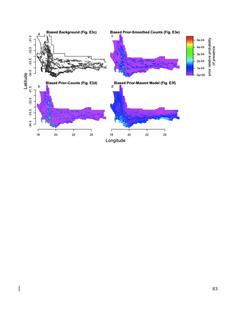
Figure C3. Background selection

The effect of different choice of background points for P. punctata using the 13 relatively uncorrelated

predictors described in Appendix 2. All settings not related to background sample selection were left

at default values for simplicity. Different numbers of background points for (a-c) were selected from

the entire CFR to illustrate how predictions can be sensitive to background selection: (a) 100; (b)

1,000; (c) 5000; (d) 10,000 (MaxEnt’s default). Using too few background points can be an issue when

(1) there are few locations in the study region (the geographic extent is small or spatial resolution is

coarse), (2) there are many locations, and the default value of 10,000 background samples does not

sufficiently cover the ecological gradients, or (3) using a biased background sample based on target

group sampling to account for sampling bias. In (e-f), background was selected from (e) a convex hull

encompassing P. punctata’s range; (f) fynbos in Cape Floristic Region. AUC values are provided to

indicate each model’s ability to discriminate presences from background locations but should not be

  

59 

compared among models because different data sets are used to calculate AUC for each model. It is not

appropriate to evaluate models with different backgrounds with a single data set when those

backgrounds represent different hypotheses. Note how predictions become more uniform when using

fewer background points or when background is selected from a larger spatial extent.

  

60 

Appendix 4: Feature Selection and Regularization

MaxEnt is designed to use all features from a given feature class or none at all. If interest lies in

using only a handful of specific nonlinear features, these features can be constructed outside of the

MaxEnt software package and provided to MaxEnt as if they were predictors. Selecting only linear

features in MaxEnt’s settings and setting the regularization coefficients to zero ensures that only these

features will be used in model construction.

For complex models, the coefficients in eqn. (6) cannot be found analytically, so MaxEnt uses a

numerical algorithm to approximate the solution. To maximize the gain, MaxEnt begins with all

coefficients set to zero and uses a greedy stepwise algorithm that at each step: (1) approximates the

lower bound for the increase in gain for each possible feature (Steven Phillips; pers. com.); (2) selects

the feature that is most likely to increase the gain; (3) proposes a new coefficient value for this feature;

(4) accepts the value if it increases the gain (Dudik et al. 2004). In principle, this approach will find the

best possible model given sufficient time. But to reduce computation time, MaxEnt uses a convergence

threshold to terminate the search procedure when changes in the gain fall below a specified threshold.

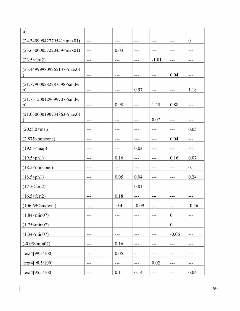
Table D1. Coefficients for models of different complexity

Models correspond to those in Figure D3. Five-fold cross-validation was used for each model; the

results from the first fold of the model with only linear and quadratic features is shown while the

results for all five folds from the model with default features is shown. By comparing the features

retained in each model, it is apparent that very different features and coefficients are chosen for models

with different complexity. Note that coefficients change considerably among models fit to different

subsets of the data (obtained during 5-fold cross validation), which is a sign of overfitting. The model

  

61 

uses many fewer features with linear and quadratic terms compared to the models with default features,

although the spatial predictions are rather similar (Fig. D3). Coefficients with values of 0 in the table

were retained by the model but had values <0.01 and were rounded to 0 for simplicity of presentation.

Feature naming follows conventions in the MaxEnt ‘lambdas file’ (see MaxEnt’s documentation for

details), except that hinge features use brackets to indicate the lower and upper bounds on the hinges.

Predictor names are explained in Table B1.

  

62 

Feature

Linear, Quadratic Features

Linear, Quadratic, Product, Threshold, Hinge Features

fold=1 fold = 1

fold = 2

fold = 3

fold = 4

fold = 5

text4^2 --- 0.05 0.18 0.42 0.24 ---

text4 --- 0.07 --- -0.09 0.18 0.1

text3^2 --- --- --- --- --- 0.22

text3*text4 --- -0.16 -0.18 -0.27 -0.23 -0.27

text3 -0.39 0.17 --- --- --- ---

text2^2 -0.01 --- --- --- --- ---

text2*text4 --- -0.64 -0.86 -0.44 -0.65 -0.69

text2*text3 --- -0.42 --- -0.25 -0.51 -0.47

text2 2.51 --- --- --- --- ---

text1^2 -0.49 0.32 --- -0.22 --- ---

text1*text4 --- -0.37 -0.58 --- -0.25 -0.38

text1*text3 --- 0.07 --- 0.25 0.15 0.13

text1*text2 --- 0.6 0.42 0.34 0.69 0.44

text1 4.16 --- --- 0.15 --- ---

smdwin^2 --- 0.21 --- 0.39 0.28 ---

smdwin*text4 --- --- --- --- --- 0.25

smdwin*text2 --- --- --- 0.62 1.43 0.36

smdwin*text1 --- 0.4 0.24 --- 1.13 0.24

smdwin 1.88 --- --- --- --- ---

rainconc^2 -2.36 -0.9 -1.22 -0.77 -0.85 -1.58

rainconc*text4 --- --- --- --- --- 0.18

rainconc*text3 --- -1.09 -0.43 -1.41 -1.02 -0.77

  

63 

rainconc*text2 --- -0.46 --- 0.46 --- 0.36

rainconc*text1 --- -4.86 -4.22 -4.02 -4.46 -4.1

rainconc 0.67 --- --- -0.21 -0.04 ---

ph3^2 -3.77 -1.44 2.88 -0.89 -5.39 -3.6

ph3*text4 --- --- -4.26 --- -9.34 -9.64

ph3*text3 --- -2.68 --- 6.24 --- ---

ph3*text2 --- 3.73 7.15 11.61 7.17 19.55

ph3*text1 --- 0.54 1.61 --- --- 3.12

ph3*smdwin --- --- --- -6.18 -0.88 ---

ph3*rainconc --- -13.29 -21.51 -15.68 -17.98 -25.56

ph3 0.54 --- --- --- 1.21 ---

ph1^2 -2.31 --- 0.21 0.33 --- 0.52

ph1*text4 --- -0.26 --- --- 0.02 0.08

ph1*text3 --- --- --- -0.15 --- ---

ph1*text2 --- 0.81 --- --- --- ---

ph1*text1 --- --- 0.47 --- 0.29 ---

ph1*smdwin --- --- 0.34 -0.08 --- ---

ph1*rainconc --- --- --- 0.07 --- ---

ph1*ph3 --- 2.34 4.79 3.51 3.89 6.09

ph1 6.59 --- 0.71 0.05 0.56 0.13

min07^2 -13.01 -10.78 -11.71 -12.44 -12.14 -12.46

min07*text3 --- -2.25 -1.44 -0.43 -1.44 -1.44

min07*text2 --- -1.44 --- -1.99 -0.49 -0.84

min07*text1 --- -2.06 --- --- --- ---

min07*smdwin --- 4.68 4.3 4.36 2.64 4.03

min07*ph3 --- -1.05 -12.17 -15.46 -10.37 -33.03

  

64 

min07 -0.19 --- -0.69 --- --- -1.96

max01^2 -2 -0.7 --- --- -0.44 ---

max01*text4 --- 0.6 --- --- --- ---

max01*text2 --- --- -0.06 --- -0.28 ---

max01*text1 --- --- 0.39 0.52 0.32 0.78

max01*rainconc --- --- --- -0.06 --- ---

max01*ph3 --- --- --- --- 2.53 0.9

max01*min07 --- -3.54 -1.7 -3.48 -1.79 -0.56

max01 --- --- -0.23 --- -0.51 -1.07

map^2 -1.8 --- --- --- --- ---

map*text4 --- -2.12 -1.71 -1.49 -1.82 -1.53

map*text3 --- 1.2 0.69 1.75 1.64 0.81

map*text2 --- 0.93 1.21 -0.22 --- 1.02

map*text1 --- 6.11 5.82 5.24 4.42 5.33

map*rainconc --- --- --- --- 0.15 0.33

map*ph3 --- --- --- --- 3.35 ---

map*ph1 --- --- --- --- -0.4 -1.01

map -0.3 --- --- --- --- ---

fert3^2 -2.49 --- --- -0.31 -0.62 -0.83

fert3*text4 --- 1.8 3.23 0.52 3.04 1.08

fert3*text3 --- -3 -4.06 -4.41 -1.73 -3.13

fert3*text2 --- -1.08 -0.49 -1.14 -1.58 -1.32

fert3*text1 --- 0.87 2.51 --- 0.38 -1.99

fert3*rainconc --- -1.4 --- -1.86 -2.12 -0.36

fert3*ph3 --- 9.52 11.84 10.14 10.45 11.58

fert3*ph1 --- 0.98 1.17 1.41 1.52 0.29

  

65 

fert3*min07 --- 4.31 --- 5.21 5.9 5.33

fert3*max01 --- --- --- --- -0.48 ---

fert3*map --- --- 0.92 1.1 0.4 1.5

fert3 3.82 --- --- --- --- ---

fert2^2 -11.14 -2.75 -5.69 -3.65 -8.78 -7.41

fert2*text4 --- 4.21 4.44 --- --- 4

fert2*text3 --- --- -4 3.22 --- ---

fert2*text2 --- --- 0.92 --- --- ---

fert2*text1 --- -4.24 -5.64 -5.25 -4.17 -12.41

fert2*smdwin --- --- --- --- -1.62 ---

fert2*rainconc --- --- 2.21 --- --- ---

fert2*ph3 --- -48.39 -53.32 -32.56 -20.47 -21.73

fert2*ph1 --- --- -0.74 -1.9 -1.36 -3.3

fert2*min07 --- -2.02 --- --- --- ---

fert2*max01 --- -0.28 --- --- --- ---

fert2*map --- 3.07 7.04 2.77 13.39 11.14

fert2*fert3 --- -1.55 --- 1.1 -7.02 -4.9

fert2 3.63 -0.39 -0.28 --- --- ---

`text4[0/6.5] --- --- --- --- -0.06 ---

`text3[0/0.5] --- --- --- --- --- 0.02

`smdwin[14.839/48.061] --- -0.18 --- --- --- ---

`smdwin[14.839/47.831] --- --- --- --- --- -0.18

`smdwin[14.839/47.806] --- --- --- --- -0.12 -0.2

`smdwin[14.839/47.794] --- --- --- --- -0.31 ---

`smdwin[14.839/28.728] --- --- --- 0.12 --- ---

`rainconc[0/7.875] --- -1.04 -1.21 -1.23 -0.68 -0.47

  

66 

`rainconc[0/5.667] --- --- -0.68 -0.44 --- ---

`rainconc[0/5.167] --- --- --- --- --- -0.75

`rainconc[0/4.833] --- --- --- --- -0.94 -1.01

`rainconc[0/2.875] --- -0.98 -1.19 --- --- ---

`ph3[0/0.5] --- -0.05 --- --- --- ---

`ph1[0/38.5] --- --- --- --- --- -0.16

`ph1[0/30.5] --- --- --- --- --- -0.16

`ph1[0/29.5] --- --- --- -0.15 -0.08 -0.38

`ph1[0/28.5] --- --- --- -0.26 --- ---

`ph1[0/22.5] --- --- -0.14 --- --- ---

`ph1[0/20.5] --- --- -0.1 --- --- ---

`ph1[0/2.5] --- -0.8 --- --- --- ---

`ph1[0/1.5] --- -0.26 -0.31 -0.41 -0.25 -0.38

`min07[-3/-2.8] --- --- --- 0.57 0.49 ---

`min07[-3/-0.95] --- --- --- 0.12 --- ---

`min07[-3/-0.85] --- --- 0.19 --- --- 0.23

`max01[18/24.583] --- --- --- -1.09 --- ---

`map[60/402.5] --- --- --- --- --- -0.13

`map[60/398.5] --- -0.53 --- --- --- ---

`map[60/396.5] --- --- --- -0.27 --- ---

`map[60/395.5] --- --- --- -0.26 -0.56 ---

`map[60/394.5] --- --- --- --- -0.68 ---

`map[60/384.5] --- --- -1.08 --- -0.31 ---

`fert3[0/0.5] --- -0.13 -0.2 -0.23 -0.08 -0.27

`fert2[0/2.5] --- 0 --- --- --- 0.02

`fert2[0/0.5] --- --- 0.01 --- --- ---

  

67 

(75.5<fert3) --- --- --- -0.01 --- ---

(560.5<map) --- --- -0.03 --- --- ---

(555.5<map) --- -0.06 -0.01 -0.08 -0.03 ---

(52.15299987792969<smdwin) --- --- -0.02 --- --- ---

(5.549999952316284<min07) --- --- --- -0.75 -0.35 -0.6

(5.450000047683716<min07) --- -0.06 -0.53 --- --- ---

(429.5<map) --- --- -0.07 --- -0.02 ---

(40.00699996948242<smdwin) --- --- --- 0.03 --- ---

(4.75<min07) --- -0.07 --- --- --- ---

(4.450000047683716<min07) --- -0.33 --- --- --- ---

(39.5<rainconc) --- 0 --- --- --- ---

(39.44500160217285<smdwin) --- 0.02 --- --- --- ---

(39.24749946594238<smdwin) --- 0.02 --- --- --- ---

(38.25<rainconc) --- --- --- 0 --- ---

(36.95450019836426<smdwin) --- 0 --- --- --- ---

(36.29249954223633<smdwin) --- --- 0.09 0.07 0.01 ---

(350.5<map) --- 0.15 --- --- --- ---

(35.26550102233887<smdwin) --- --- 0.03 --- --- ---

(346.5<map) --- --- 0.06 0.14 --- 0.19

(343.5<map) --- --- 0.01 --- --- ---

(341.5<map) --- --- 0.05 --- --- ---

(34.60900115966797<smdwin) --- --- --- 0 --- ---

(330.5<map) --- --- 0.01 --- --- ---

(322.5<map) --- --- 0.03 --- --- ---

(32.16200065612793<smdwin) --- 0.21 --- --- --- ---

(32.13850021362305<smdwin) --- --- 0.06 0.01 --- 0.1

  

68 

(31.513999938964844<smdwin) --- 0.1 --- --- --- ---

(31.41849994659424<smdwin) --- --- --- 0.17 --- ---

(31.25<max01) --- --- -0.33 -0.38 --- -0.07

(31.016499519348145<smdwin) --- --- --- --- 0.1 0.1

(30.949999809265137<max01) --- -0.17 --- --- --- ---

(30.75<max01) --- -0.17 -0.03 --- --- ---

(3.8333334922790527<min07) --- -0.03 --- 0 --- -0.11

(3.3833335638046265<min07) --- --- --- --- 0.01 ---

(29.75<max01) --- --- --- --- 0.01 ---

(28.5<ph1) --- --- --- --- 0.05 ---

(28.321499824523926<smdwin) --- -0.24 -0.04 --- --- ---

(28.00349998474121<smdwin) --- -0.05 --- --- -0.36 -0.15

(27.480000495910645<smdwin) --- --- --- -0.06 --- ---

(26.91249942779541<max01) --- --- -0.02 -0.31 -0.06 -0.02

(26.65000057220459<max01) --- -0.03 --- --- --- -0.04

(26.541665077209473<max01) --- --- -0.01 --- --- ---

(26.5166654586792<max01) --- -0.17 -0.07 -0.05 --- -0.03

(26.5<fert2) --- --- -0.66 --- --- ---

(26.324999809265137<max01) --- --- --- --- -0.02 ---

(26.033334732055664<max01) --- --- --- --- -0.02 ---

(25.5<ph1) --- --- --- 0.17 --- ---

(25.483500480651855<smdwi --- --- --- -0.01 --- ---

  

69 

n)

(24.34999942779541<max01) --- --- --- --- --- 0

(23.65000057220459<max01) --- 0.03 --- --- --- ---

(23.5<fert2) --- --- --- -1.01 --- ---

(23.449999809265137<max01) --- --- --- --- 0.04 ---

(21.779000282287598<smdwin) --- --- 0.97 --- --- 1.18

(21.751500129699707<smdwin) --- 0.98 --- 1.25 0.88 ---

(21.050000190734863<max01) --- --- --- 0.07 --- ---

(2025.0<map) --- --- --- --- --- 0.05

(2.875<rainconc) --- --- --- --- 0.04 ---

(192.5<map) --- --- 0.03 --- --- ---

(19.5<ph1) --- 0.16 --- --- 0.16 0.07

(18.5<rainconc) --- --- --- --- --- 0.1

(18.5<ph1) --- 0.05 0.04 --- --- 0.24

(17.5<fert2) --- --- 0.01 --- --- ---

(16.5<fert2) --- 0.18 --- --- --- ---

(106.69<smdwin) --- -0.4 -0.09 --- --- -0.56

(1.84<min07) --- --- --- --- 0 ---

(1.75<min07) --- --- --- --- 0 ---

(1.34<min07) --- --- --- --- -0.06 ---

(-0.05<min07) --- 0.16 --- --- --- ---

'text4[99.5/100] --- 0.05 --- --- --- ---

'text4[98.5/100] --- --- --- 0.02 --- ---

'text4[95.5/100] --- 0.11 0.14 --- --- 0.04

  

70 

'text3[97.5/100] --- --- -0.26 -0.07 --- -0.25

'text2[98.5/100] --- -1.35 -3.17 -1.55 -1.39 ---

'text2[97.5/100] --- --- --- -0.27 --- -1.09

'text2[96.5/100] --- --- --- --- --- -0.25

'text2[87.5/100] --- --- 0.16 --- --- ---

'text2[86.5/100] --- 0.55 --- 0.84 --- ---

'text2[85.5/100] --- --- 0.65 --- --- ---

'text1[96.5/100] --- --- --- 0.98 0.76 ---

'text1[95.5/100] --- --- 0.27 --- --- 1.11

'text1[94.5/100] --- 1.1 --- --- --- ---

'smdwin[80.507/110.885] --- --- --- --- 0.01 ---

'smdwin[80.484/110.885] --- 0 --- --- --- ---

'rainconc[55.125/69] --- --- 0.54 --- --- 0.65

'ph1[98.5/100] --- -0.09 --- --- -0.04 ---

'ph1[97.5/100] --- -0.05 -0.14 -0.21 --- ---

'ph1[92.5/100] --- -0.02 --- --- --- -0.32

'ph1[91.5/100] --- --- --- --- -0.02 ---

'min07[3.667/9.2] --- -1.95 --- --- --- ---

'min07[3.617/9.2] --- --- -1.62 --- --- -0.69

'min07[3.55/9.2] --- --- --- --- -1.73 ---

'max01[30.183/33.5] --- --- --- --- --- -0.17

'max01[30.09/33.5] --- --- --- --- -0.52 ---

'max01[25.817/33.5] --- --- -0.57 --- --- ---

'max01[25.71/33.5] --- --- --- --- --- -0.27

'map[1779/3152] --- --- --- 0.29 --- ---

  

71 

Table D2. Number of Features The number of features derived from each predictor. The first and second columns indicate the

possible feature classes and their interpretations for models based on continuous predictor variables.

The third and fourth columns show the number of features from each feature class that are possible

when using default settings in a model with 19 predictors (the number of Bioclim predictors (Hijmans

et al. 2005)) and 100 presences (a representative number). The fifth column shows the number of

features retained in a default model for P. punctata (Fig. 4) using default feature selection. The number

of features is substantially lower than the number of potential features, but substantially higher than

many regression-based statistical models.

Feature

class

Constrains

the…

Bioclim

Feature

counting

# Potential

Bioclim

Features

# Features retained

in default

P. punctata model

Linear Mean 19 * 1 19 3

Quadratic Variance 19 * 1 19 8

Product Covariance 19!/17!2! 171 43

Threshold Quantiles 19*99 1881 25

Hinge Piecewise Mean 19*99*2 3762 19

  

72 

Figure D1. Examining different regularization coefficients

Plots of a number of different fit metrics versus the regularization coefficient values (β) to determine

optimal. β is a constant that MaxEnt multiplies the regularization penalty by (third term in eqn. (9)).

Dashed grey lines indicate default regularization coefficient values. All models use the 13 relatively

uncorrelated predictors to model the distribution of for P. punctata with default feature classes (Fig.

D3b). Models have optimal fit with regularization coefficients from 1-5 due to balancing overfitting

with generality; notably, higher regularization coefficients can improve fit to training data in this data

set. Similar patterns were observed by Phillips and Dudik (2008; their Fig. 2). Note that the

regularization coefficients cannot be increased indefinitely, or empirical constraints will not be

matched by the predictions (Fig. D2).

  

73 

Figure D2. Consequences of increasing regularization coefficients

Plot of the difference between predicted and observed constraints for different regularization values.

Dashed grey lines indicate default regularization coefficient values. All models use the 13 relatively

uncorrelated predictors to model the distribution of for P. punctata. Only linear features were allowed,

for the sake of simplifying the illustration. Features have been rescaled to [0,1] to make values

comparable. Constraints are not necessarily enforced when regularization coefficients are increased, as

with MAX01 or TEXT2. Regularization is valuable to ensure that constraints are not enforced too

precisely (to avoid overfitting) but because MaxEnt uses it simultaneously for feature selection, it may

be tempting to simply increase the regularization coefficients to produce simpler models. This can be

done to a point (e.g. regularization coefficients =5-10 in our experiments) but eventually constraints

may not be enforced. Since constraints interact with one another due to covariation among predictors,

it is possible for some constraints to be more precisely enforced as other constraints are relaxed, as

with MIN07 or RAINCONC here, which may be a sign of overly correlated predictors.

  

74 

● ● ●

●●

●●

●

●

●

●

0 1 0 5 2 0 10 0 50 0

0 086

0 087

0 088

0 089

0 090

fert3

●● ●

●

●

●

●

●

●

●

●

0 1 0 5 2 0 10 0 50 0

0 3765

0 3770

0 3775

0 3780

0 3785

0 3790

map

● ● ●●

●

●

●●

●

●

●

0 1 0 5 2 0 10 0 50 0

0 385

0 390

0 395

0 400

0 405

0 410

min07

● ● ●●

●

●●

●

●

●

●

0 1 0 5 2 0 10 0 50 0

0 388

0 390

0 392

0 394

0 396

rainconc

●● ●

●●

● ●

●

●

●

●

0 1 0 5 2 0 10 0 50 0

0 631

0 632

0 633

0 634

smdwin

● ● ●●

●

●

●●

●

●

●

0 1 0 5 2 0 10 0 50 0

0 08

0 09

0 10

0 11

max01

● ● ● ● ●● ●

●

●

●

●

0 1 0 5 2 0 10 0 50 0

0 001

0 002

0 003

0 004

fert2

●●

●●

●

●●● ●

●●

0 1 0 5 2 0 10 0 50 0

0 2975

0 2980

0 2985

0 2990

0 2995

0 3000

0 3005

ph1

● ● ●●

●

●

●

●

●

●

●

0 1 0 5 2 0 10 0 50 0

0 006

0 007

0 008

0 009

0 010

0 011

0 012

ph3

● ● ● ●●

●●

●

●

●

●

0 1 0 5 2 0 10 0 50 0

0 004

0 005

0 006

0 007

0 008

0 009

0 010

text1

● ● ● ● ●●

●

●

●

●

●

0 1 0 5 2 0 10 0 50 0

0 010

0 015

0 020

0 025

0 030

0 035

text2

● ● ●

●

●

●

●●

●

●

●

0 1 0 5 2 0 10 0 50 0

0 152

0 154

0 156

0 158

0 160

0 162

text3

● ●●

●

●

●

●●

●

●

●

0 1 0 5 2 0 10 0 50 0

0 160

0 162

0 164

0 166

0 168

0 170

0 172

text4

  

75 

Figure D3. Predicted Distribution with Different Feature Classes

MaxEnt predictions for P. punctata (a-b) and P. lacticolor (c-d). (a) and (c) show models using only

linear and quadratic features while (b) and (d) use all feature classes. Mean (standard deviation) AUC

was calculated on test and training data using 5-fold cross validation. Predictions are very similar

between the simpler and more complex models. More complex models often have a larger difference

between test and training AUC values than simpler models, which is an indication of overfitting. Note

that the relative probability values are much lower for a more wide-ranging species like P. punctata

than a narrow-ranging species like P. lacticolor, because much of the probability is concentrated in just

a few locations in the latter case. This illustrates a challenge in comparing MaxEnt models for different

species unless the predictions are transformed (see section III.E), which carries with it additional

assumptions.

  

76 

  

77 

Appendix 5: Sampling Bias

Sampling bias is defined with respect to the landscape of interest. For example, the Protea

distributions from our case study are well sampled across large climatic gradients (e.g. Southern

Africa, or the CFR) that accurately define the distribution, but may still be poorly sampled at fine

(<1km) spatial scales, for a few species that are narrowly confined to small areas of limestone or shale

outcrops (cf. Rebelo 2001). Since the landscape is defined by the background extent, which should be

chosen based on ecological questions (Section III.A), the importance of sampling bias can be

intertwined with the study objectives (Anderson 2012).

Table E1. Biased Prior

Demonstration of accounting for sampling bias with the biased prior method. Models were built using

only the linear and quadratic features shown, with regularization turned off. Let s(x) denote the

sampling effort in location x. s(x) is a multinomial distribution in geographic space that describes the

proportion of the total sampling effort in each location. If s(x) is taken as the prior (in eqn. 6 in the

main text), it reflects the null hypothesis that the species is equally likely to occur everywhere and that

the relative probability of finding the species is only related to the search effort in the location (and not

the environment). When the prior is set equal to s(x), MaxEnt predicts the distribution P*(z(x))s(x)

rather than P*(z(x)) (Dudik et al. 2005). Sampling bias can be factored out of this result and, once

normalized, provide an estimate of P*(z(x)). Consider the landscape and occurrence data in Fig. 2f.

The table shows how different predictions emerge had four different sampling schemes produced these

data. Sampling Scheme 1 corresponds to no sampling bias, and produces MaxEnt’s default prediction.

For Sampling Scheme 2, we assume that sampling was biased toward warmer locations, and find that

predicted probability in colder locations increases relative to sampling scheme 1. Sampling Scheme 3

  

78 

is biased toward colder locations, which upweights the predictions at warmer locations. Sampling

Scheme 4 represents the scenario where locations with MJT = 0 were not sampled or sampled much

less than other locations. In such cases it is necessary to assign arbitrarily small values of sampling to

these locations because the prior appears in the denominator of eqn. 1 and values of zero are not

permitted. These values should be chosen cautiously, however, because dividing by a very small

number can substantially upweight predictions to produced nonsensical results. Note that the

predictions are highest in locations with MJT = 0, in spite of the fact that no presences have been

observed there. Further research is needed to determine the best way to deal with locations with little

or no sampling effort.

  

79 

Data Sampling Scheme 1 Sampling Scheme 2 Sampling Scheme 3 Sampling Scheme 4

Loc

atio

n

Feat

ure

1 (M

JT)

Feat

ure

2 (M

JT2 )

Pres

ence

Prio

r s(

z)

P*(z

(x))*s(z)

Pred

ictio

n

P*(z

(x)

Prio

r

s(z)

P*( z

(x)*s(z)

Pred

ictio

n

P*(z

(x)

Prio

r s(

z)

P*( z

(x)*s(z)

Pred

ictio

n

P*(z

(x)

Prio

r

s(z)

P*( z

(x)*s(z)

Pred

ictio

n

P*(z

(x)

1 0 0 0 0.167 0.019 0.019 0.100 0.031 0.057 0.300 0.024 0.008 0.001 0.017 0.434 2 0 0 0 0.167 0.019 0.019 0.100 0.031 0.057 0.300 0.024 0.008 0.001 0.017 0.434 3 1 1 1 0.167 0.137 0.137 0.100 0.063 0.116 0.100 0.109 0.112 0.100 0.149 0.038 4 2 4 1 0.167 0.307 0.307 0.300 0.343 0.211 0.100 0.321 0.331 0.399 0.300 0.019 5 2 4 1 0.167 0.307 0.307 0.300 0.343 0.211 0.100 0.321 0.331 0.399 0.300 0.019 6 3 9 1 0.167 0.212 0.212 0.100 0.188 0.347 0.100 0.203 0.209 0.100 0.216 0.055

  

80 

Figure E1. Distribution of predictors at CFR and Protea Atlas locations

Comparing the distribution of environmental conditions across the CFR to those sampled during the

Protea Atlas enables assessment of sampling bias. The predictor variables represent the suite of

candidate predictors with correlation <0.64. This approach relies on the assumption of target group

sampling: the Protea Atlas locations represent the suite of locations searched for P. punctata and P.

lacticolor. With the exception of fertility class 2 and PH class 1, the sampling appears unbiased, based

on visual inspection. Note that we have not evaluated the multivariate environmental surface, so it is

possible that unique combinations of the predictors that exist in the CFR have not been well sampled

by the Protea Atlas. Existing studies have relied on visual comparisons among TGS and landscape

locations, however quantification is possible using Ali-Silvey distances (a.k.a. f-divergences; Ali and

Silvey 1966) designed to measure the overlap of two probability distributions (of which relative

entropy is one example). Predictor’s codes are described in Table B1.

  

81 

  

82 

Figure E2. Bias background and priors

Shown here is the information used to account for sampling bias in Figure E3. (a) Biased background;

points represent the locations of sampled locations. (b) Biased prior; locations sampled during the

Protea Atlas were used to construct a prior distribution to reflect sampling effort, based on the number

of Atlas records in each location (counts). By using the number of records in a grid cell (rather than

simply indicating sampled versus unsampled) we modeled variation sampling effort among sampled

cells. To build this model, we used the number of observations in the Protea Atlas database in each

grid cell, and divided this value by the total number of counts to produce a normalized surface. (c)

Biased prior; same as (b) but using smoothing the surface by averaging the value in a location with its

eight nearest neighbors. This approach might be desirable to account for nearby locations (d) Biased

prior; using a model for search effort based on elevation and distance to urban centers and distance to

roads.

  

83 

  

84 

Figure E3. Predictions for different sampling bias methods

All models were built using the suite of 13 relatively uncorrelated features described in Appendix 2.

Sampling bias was not a problem for the Protea Atlas data at the 1’ scale (Fig. E1), so we subsampled

the Atlas locations (background) and P. punctata presences to artificially create bias in the presence

sample along the minimum July temperature gradient. See Fig. E4 for an illustration of the artificial

sampling bias and more detailed methods. Since this artificial sampling scheme tends to omit the

eastern part of P. punctata’s range, we zoom in on the predictions there to compare how

accounting/ignoring sampling bias there affects predictions. (a) The best model (the ‘truth’), using the

complete, unbiased data set. The various methods of accounting for bias in (b)-(f) can do no better than

(a), so we measured the difference between each model and (a) using the Kullback-Leibler divergence

(denoted KL). A value of 0 indicates perfect agreement, with larger values indicating increasing

disagreement. (b) Model built with biased presences that ignores sampling bias, illustrating the

incorrect predictions that can emerge when bias is ignored. (c-e) Various methods to incorporate

sampling bias based on target group sampling. (c) Biased background; only locations sampled during

the Protea Atlas are used as background. Note that these background locations were artificially

subsampled to contain the same bias as the presence data, so we expect that they should be suitable for

accounting for sampling bias. (d) Biased prior; locations sampled during the Protea Atlas were used to

construct a prior distribution to reflect sampling effort, based on the number of Atlas samples recorded

in each location (counts). (e) Biased prior; same as (d) but smoothing the surface by averaging the

value in a location with its eight nearest neighbors. (f) Biased prior; using a model for search effort

built with MaxEnt. We used the (artificially biased) background sample from the Protea Atlas to model

the search effort as a function of the environmental predictors. This model accurately characterized our

  

85 

artificial subsampling scheme along the MJT gradient, as indicated by a value of 84 for the

permutation importance of MJT provided by MaxEnt. It is not surprising that the method to account

for sampling bias was the most successful because our artificial subsampling scheme was explicitly

biased along the MJT gradient; such bias may not be so simple to model in real data sets. All methods

to account for bias improve predictions over the model that ignores bias.

  

86 

Figure E4. P. punctata bias histograms

To illustrate the consequences of ignoring sampling bias we subsampled the P. punctata presences and

Protea Atlas locations in biased fashion to simulate a biased data set. A biased sample was selected

along the Minimum July Temperature (MJT) gradient because P. punctata exhibits a strong response

to it. To bias the sample toward warmer MJT, a sample was obtained from randomly selecting

locations with probability proportion to the MJT raised to the fourth power. The bias is illustrated by

the histograms, which compare the distribution of MJT at background locations in the true and biased

samples to their distribution among the presence locations. Both the biased background and presence

sample exhibit a similar shift toward warmer MJT compared to the true samples, so we expect that by

predictions can be improved for the biased sample using target groups sampling (Fig. E3).

  

87 

Finally, we note a few technical points that may be helpful for understanding sampling bias. First,

one should not expect the gain to improve by incorporating bias in to the model. Phillips et al. (2009)

observed that gain often decreases when sampling bias is incorporated, but that AUC on test data

increases. When sampling is highly correlated with a predictor, that predictor will have a large

coefficient in a model where sampling bias is ignored. However, if this predictor does not actually

influence the species distribution, factoring out sampling bias will reduce this coefficient and reduce

MaxEnt’s ability to differentiate the presences from the background in training data. Accounting for

sampling bias should improve prediction on test data because it removes spurious features that are

related to the sampling bias, and not the species distribution.

  

88 

Appendix 6: Types of Output

Note that if raw output is generated using different numbers of background points across the same

landscape (cf. Fig. A1), the values must be normalized to make comparisons among models.

Figure F1. Variation in predictions using different values of τ

The value of tau is related to the prevalence of the species (the proportion of locations in the landscape

where the species occurs; Phillips and Dudik (2008)). By default, MaxEnt uses tau = 0.5 to produce

logistic output. Phillips and Dudik (2008) propose interpreting the logistic output as the absolute

probability of presence, be we caution against this because predictions are very sensitive to the

assumption that tau = 0.5.

  

89 

Figure F2. Variation in visual appearance of different output formats

Five different displays of model output for the same model for P. lacticolor. The left column shows

output on a linear color scale, while the right column shows coloration on a log scale. The first row

shows raw output, the second row show cumulative output and the third row shows logistic output.

Notice how relatively minimal difference among the best locations under raw output (in red) are

stretched out over the color scale using cumulative output, making the range appear substantially

larger.

!"#$%&'()*)&'+,%*$'' ' ' ' ' '!)-'()*)&'+,%*$ ''

''

''./01/

0'2)&3%0'

!)-"45,

''

''(/3

/*%5

6$'

''7%8

''

  

90 

Appendix References

Ali, S. and Silvey, S. 1966. A general class of coefficients of divergence of one distribution from

another. — Journal of the Royal Statistical Society. Series B (Methodological) 28: 131-142.

Anderson, R. P. 2012. Harnessing the world's biodiversity data: promise and peril in ecological niche

modeling of species distributions. — Annals of the New York Academy of Sciences 1260:66–

80.

Elith, J. et al. 2010. The art of modelling range-shifting species. — Methods in Ecology and Evolution

1: 330-342.

Engler, R. and Guisan, A. 2009. MigClim: Predicting plant distribution and dispersal in a changing

climate. — Diversity and Distributions 15: 590-601.

Guisan, A. and Zimmermann, N. 2000. Predictive habitat distribution models in ecology. —

Ecological Modelling 135: 147-186.

Latimer, A. et al. 2006. Building statistical models to analyze species distributions. — Ecological

Applications 16: 33-50.

Merow, C. et al. 2011. Developing Dynamic Mechanistic Species Distribution Models: Predicting

Bird-Mediated Spread of Invasive Plants across Northeastern North America. — The American

Naturalist 178: 30-43.

Phillips, S. and Dudik, M. 2008. Modeling of species distributions with MaxEnt: new extensions and a

comprehensive evaluation. — Ecography 31: 161.

Phillips, S. et al. 2009. Sample selection bias and presence-only distribution models: implications for

background and pseudo-absence data. — Ecological Applications 19: 181-197.

  

91 

Warren, D. L. et al. 2008. Environmental niche equivalency versus conservatism: quantitative

approaches to niche evolution. — Evolution; international journal of organic evolution 62: 2868-2883.