ECON 497 Final Exam Page 1 of 12
ECON 497: Economic Research and Forecasting Name:________________
Spring 2008 Bellas
Final Exam
Return this exam to me by 4:00 on Wednesday, April 23. It may be e-mailed to me. It
may be delivered to my office in Minneapolis or faxed to me before 4:00 on the 25th
at
612-659-7268. You could even drop it by my house if you like, and I’d be pleased to
introduce you to my wife and my kids. You can also send it to my office through the
regular post or to my home via regular post, but it should be post-marked by the 23rd.
You may consult any written source you like regarding the answers to these questions but
you may not ask any person other than me any questions about this test. Questions to me
must be sent via e-mail and responses will be sent to the entire class.
Answer all questions, and explain your answers. Fifty points total, points per part
indicated in parentheses.
1. It will probably come as no surprise to you that economists love a good fight.
Graduate school was a long series of scuffles, brawls and flat out donnybrooks. Happily,
we always noted who was involved and, more importantly, who won. We estimated a
binomial logit model of the fight outcomes and came up with the following:
𝑙𝑛 𝑃 𝑖
1−𝑃 𝑖 = −1.9 + 0.4𝐹𝑖 + 0.2𝑀𝐼𝑖 + 0.01𝐴𝑖
Where Fi is a female dummy variable, MIi is a microeconomist dummy and Ai is the age
of the participant in question.
A. Without knowing any of the characteristics of his opponent (an admitted weakness of
the model) calculate the probability that a 40 year old male microeconomist will win a
fight. (3)
1
1 + 𝑒−(−1.9+0.4 0 +0.2 1 +0.01 40 )=
1
1 + 𝑒1.3=
1
1 + 3.7= 0.2128
B. This is a bit trickier. Based on this model and assuming that no econ fight ever ended
in a tie, discuss how you might arrive at the probability a 25 year old male
macroeconomist would win a fight against a 50 year old female microeconomist.
Remember, and this is the trick, that there are no ties and that the probability of all
possible outcomes must sum to one. (2)
𝟏
𝟏 + 𝒆−(−𝟏.𝟗+𝟎.𝟒 𝟎 +𝟎.𝟐 𝟎 +𝟎.𝟎𝟏 𝟐𝟓 )=
𝟏
𝟏 + 𝒆𝟏.𝟔𝟓=
𝟏
𝟏 + 𝟓.𝟐𝟎𝟕= 𝟎.𝟏𝟔𝟏𝟏
𝟏
𝟏+ 𝒆−(−𝟏.𝟗+𝟎.𝟒 𝟏 +𝟎.𝟐 𝟏 +𝟎.𝟎𝟏 𝟓𝟎 )=
𝟏
𝟏+ 𝒆𝟎.𝟖=
𝟏
𝟏+ 𝟐.𝟐𝟐𝟓𝟓= 𝟎.𝟑𝟏𝟎𝟎
ECON 497 Final Exam Page 2 of 12
You might say that the probability that either one of these economists wins the fight
is equal to their probability divided by the sum of the predicted probabilities. So,
for the 25 year old male macroeconomist, the predicted probability would be:
𝟎.𝟏𝟔𝟏𝟏
𝟎.𝟏𝟔𝟏𝟏+𝟎.𝟑𝟏𝟎𝟎=
𝟎.𝟏𝟔𝟏𝟏
𝟎.𝟒𝟕𝟏𝟏= 𝟎.𝟑𝟒𝟐
2. Use the coffee data from assignment #2 to estimate the attendance elasticity of coffee
demand (basically
𝑑𝐶𝑡𝐶𝑡𝑑𝐴 𝑡𝐴𝑡
or, if you prefer, %∆𝐶
%∆𝐴 ). You should also include the other
explanatory variables in your model.
To do this you need to regress the natural log of coffee sales on the natural log of
attendance. You should also include the other explanatory factors as well.
A. Present your results. (2)
SUMMARY OUTPUT
Regression Statistics Multiple R 0.643815 R Square 0.414497 Adjusted R Square 0.391686 Standard Error 0.102851 Observations 81
ANOVA df SS MS F
Regression 3 0.576638 0.192213 18.17032
Residual 77 0.814536 0.010578 Total 80 1.391174
Coefficients Standard
Error t Stat P-value
Intercept 8.565642 0.420669 20.36193 9.9E-33
lnA 0.250342 0.036715 6.818522 1.83E-09
lnT -0.22716 0.060034 -3.78389 0.000304
N 0.01227 0.024091 0.509322 0.611983
The elasticity is the estimated coefficient on ln(A), which is 0.250342. You might
also have done this with T instead of lnT as an explanatory variable and gotten the
following:
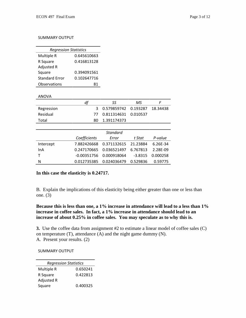
ECON 497 Final Exam Page 3 of 12
SUMMARY OUTPUT
Regression Statistics Multiple R 0.645610663 R Square 0.416813128 Adjusted R
Square 0.394091561 Standard Error 0.102647716 Observations 81
ANOVA df SS MS F
Regression 3 0.579859742 0.193287 18.34438
Residual 77 0.811314631 0.010537 Total 80 1.391174373
Coefficients Standard
Error t Stat P-value
Intercept 7.882426668 0.371132615 21.23884 6.26E-34
lnA 0.247170665 0.036521497 6.767813 2.28E-09
T -0.00351756 0.000918064 -3.8315 0.000258
N 0.012735385 0.024036479 0.529836 0.59775
In this case the elasticity is 0.24717.
B. Explain the implications of this elasticity being either greater than one or less than
one. (3)
Because this is less than one, a 1% increase in attendance will lead to a less than 1%
increase in coffee sales. In fact, a 1% increase in attendance should lead to an
increase of about 0.25% in coffee sales. You may speculate as to why this is.
3. Use the coffee data from assignment #2 to estimate a linear model of coffee sales (C)
on temperature (T), attendance (A) and the night game dummy (N).
A. Present your results. (2)
SUMMARY OUTPUT
Regression Statistics Multiple R 0.650241 R Square 0.422813 Adjusted R
Square 0.400325
ECON 497 Final Exam Page 4 of 12
Standard Error 2780.661 Observations 81
ANOVA df SS MS F
Regression 3 4.36E+08 1.45E+08 18.80188
Residual 77 5.95E+08 7732074 Total 80 1.03E+09
Coefficients Standard
Error t Stat P-value
Intercept 24876.39 2006.804 12.39602 4.99E-20
N 412.3307 651.3658 0.633025 0.528593
T -86.5844 24.74468 -3.49911 0.000779
A 0.253492 0.036882 6.872992 1.44E-09
B. Do a Park test for heteroskedasticity and discuss the results of this test. (3)
To do a Park test you need to save the residuals from the original regression and
then square them and take the natural log of the squared residuals and then regress
the log of the squared residuals on the explanatory factor that you think is
responsible for the heteroskedasticity, which, in this case, is likely to be attendance.
So, we estimate the model: ln(ei2) = B0 + B1*ln(A) + ε
Here are the results.
SUMMARY OUTPUT
Regression Statistics Multiple R 0.358803 R Square 0.128739 Adjusted R
Square 0.117711 Standard Error 1.597605 Observations 81
ANOVA df SS MS F
Regression 1 29.794 29.794 11.6732
Residual 79 201.635 2.552342 Total 80 231.429
ECON 497 Final Exam Page 5 of 12
Coefficients Standard
Error t Stat P-value
Intercept -4.63092 5.746775 -0.80583 0.42276
lnA 1.92464 0.563319 3.416607 0.001004
The estimated coefficient on lnA is significantly different from zero which suggests
that there is heteroskedasticity.
4. The best way to determine if there is multicollinearity in your model is to calculate (or
ask a software package to calculate) VIFs for the explanatory variables. Explain
carefully where these VIF numbers come from. (3)
A VIF is derived from the R-squared value that results from regressing one
explanatory variable on all other explanatory variables. The VIF is equal to
𝑽𝑰𝑭 =𝟏
𝟏−𝑹𝟐
5. There is data on real personal consumption spending (in billions of year 2000 dollars)
and population for the U.S. available on the course web site. The data are from
Microeconomics: Principle and Policy, 10th
edition, by William J. Baumol and Alan S.
Blinder. Use this data to do the following.
A. Estimate a linear model of real consumption spending as a function of population and
year. Briefly discuss your results. (2)
SUMMARY OUTPUT
Regression Statistics Multiple R 0.995448 R Square 0.990917 Adjusted R
Square 0.990349 Standard Error 149.0443 Observations 35
ANOVA df SS MS F
Regression 2 77550865 38775432 1745.523
Residual 32 710854.8 22214.21 Total 34 78261719
Coefficients Standard t Stat P-value
ECON 497 Final Exam Page 6 of 12
Error
Intercept 211092.1 53692.6 3.931493 0.000424
Year -116.363 28.35483 -4.10381 0.000261
Population 100.1613 10.80105 9.273298 1.39E-10
Population is in hundred millions, so this suggests that an additional hundred
million people will increase spending by about 100 billion dollars, or that an extra
person will increase spending by about $1000 and that, adjusting for population,
spending decreases by about 116 billion dollars per year.
B. Is there evidence of serial correlation in your model in part A? Offer three different
pieces of supporting evidence. (3)
Here is a scatterplot of the residuals:
This suggests that there is serial correlation because there are long periods of either
positive or negative residuals.
Here are the results of a regression of residuals on lagged residuals:
SUMMARY OUTPUT
Regression Statistics Multiple R 0.83709 R Square 0.70072 Adjusted R
Square 0.691066 Standard Error 82.68103
-300
-200
-100
0
100
200
300
400
1965 1970 1975 1980 1985 1990 1995 2000 2005 2010
ECON 497 Final Exam Page 7 of 12
Observations 33
ANOVA df SS MS F
Regression 1 496181.5 496181.5 72.58197
Residual 31 211920.7 6836.153 Total 32 708102.2
Coefficients Standard
Error t Stat P-value
Intercept 7.79131 14.43508 0.539748 0.593227
Lag Resid 0.896052 0.105177 8.519506 1.27E-09
The significant estimated coefficient suggests that there is serial correlation.
You could also calculate a Durbin-Watson statistic. Here is the output from doing
this in the statistical analysis package Stata:
. reg consumption year population
Source | SS df MS Number of obs = 35
-------------+------------------------------ F( 2, 32) = 1745.52
Model | 77550861.9 2 38775431 Prob > F = 0.0000
Residual | 710855.15 32 22214.2234 R-squared = 0.9909
-------------+------------------------------ Adj R-squared = 0.9903
Total | 78261717.1 34 2301815.21 Root MSE = 149.04
------------------------------------------------------------------------------
consumption | Coef. Std. Err. t P>|t| [95% Conf. Interval]
-------------+----------------------------------------------------------------
year | -116.3628 28.35483 -4.10 0.000 -174.1197 -58.60591
population | 100.1613 10.80105 9.27 0.000 78.16029 122.1623
_cons | 211091.9 53692.59 3.93 0.000 101723.7 320460.1
------------------------------------------------------------------------------
. estat dwatson
Durbin-Watson d-statistic( 3, 35) = .3147575
The D-W value of 0.3147575 is close to zero, suggesting that there is positive serial
correlation.
C. Estimate a semi-log model in which the dependent variable is the natural log of per
capita consumption spending and the explanatory variable is year. Present your results.
(2)
Here are the results from Stata:
. reg lnpercap year
Source | SS df MS Number of obs = 35
ECON 497 Final Exam Page 8 of 12
-------------+------------------------------ F( 1, 33) = 3363.12
Model | 1.71362853 1 1.71362853 Prob > F = 0.0000
Residual | .016814676 33 .000509536 R-squared = 0.9903
-------------+------------------------------ Adj R-squared = 0.9900
Total | 1.73044321 34 .050895389 Root MSE = .02257
------------------------------------------------------------------------------
lnpercap | Coef. Std. Err. t P>|t| [95% Conf. Interval]
-------------+----------------------------------------------------------------
year | .0219091 .0003778 57.99 0.000 .0211405 .0226777
_cons | -40.6672 .7506831 -54.17 0.000 -42.19448 -39.13992
------------------------------------------------------------------------------
D. What is the interpretation of the estimated coefficient on year in the model in part C?
(2)
The interpretation is that per capita consumption increases by about 2.19%
annually.
E. Estimate a generalized least squares (GLS) model to correct for the serial correlation
in your model from part C. Show clearly how you estimate the GLS model and present
your results. (2)
Starting with the D-W stat of 0.3147575 we can calculate an estimate of rho….
𝝆 = 𝟏 −𝑫𝑾
𝟐= 𝟏 −
𝟎.𝟑𝟏𝟒𝟕𝟓𝟕𝟓
𝟐= 𝟎.𝟖𝟒𝟐𝟔
So we recalculate the dependent variable as 𝒍𝒏𝒑𝒆𝒓𝒄𝒂𝒑𝒕 − 𝟎.𝟖𝟒𝟐𝟔 ∙ 𝒍𝒏𝒑𝒆𝒓𝒄𝒂𝒑𝒕−𝟏
and we recalculate the explanatory variable, year, as 𝒚𝒆𝒂𝒓𝒕 − 𝟎.𝟖𝟒𝟐𝟔𝒚𝒆𝒂𝒓𝒕−𝟏 and
then re-do the regression with these new dependent and explanatory variables.
Here are the results as reported in Stata:
. reg glsdepvar glsexplvar
Source | SS df MS Number of obs = 34
-------------+------------------------------ F( 1, 32) = 156.09
Model | .039263451 1 .039263451 Prob > F = 0.0000
Residual | .008049591 32 .00025155 R-squared = 0.8299
-------------+------------------------------ Adj R-squared = 0.8245
Total | .047313042 33 .001433729 Root MSE = .01586
------------------------------------------------------------------------------
glsdepvar | Coef. Std. Err. t P>|t| [95% Conf. Interval]
-------------+----------------------------------------------------------------
glsexplvar | .0220064 .0017614 12.49 0.000 .0184185 .0255944
_cons | -6.430733 .5525263 -11.64 0.000 -7.556193 -5.305274
------------------------------------------------------------------------------
ECON 497 Final Exam Page 9 of 12
. estat dwatson
Durbin-Watson d-statistic( 2, 34) = 1.248493
The new Durbin-Watson statistic of 1.248 suggests that serial correlation is less of a
problem than it was before. The estimated coefficient on year (the GLS explanatory
variable, glsexplvar) is still 0.022 but the t-stat has fallen to 12.49.
6. Use the Age-Wisdom data that is available on the web site to do some stuff.
A. Estimate a pooled model in which wisdom is the dependent variable and age is the
explanatory variable. Present your results. (3)
SUMMARY OUTPUT
Regression Statistics Multiple R 0.578256 R Square 0.33438 Adjusted R
Square 0.32926 Standard Error 7.588247 Observations 132
ANOVA df SS MS F
Regression 1 3760.458 3760.458 65.30671
Residual 130 7485.594 57.5815 Total 131 11246.05
Coefficients Standard
Error t Stat P-value
Intercept 1.824308 2.387246 0.76419 0.446139
Age 0.673956 0.083397 8.081256 3.85E-13
B. Briefly discuss your results from part A. (3)
The pooled results suggest that wisdom increases with age.
C. Estimate a fixed-effects model in which wisdom is the dependent variable. Present
your results. (3)
To do this in SPSS or Excel, you need to create a dummy variable for each person.
SUMMARY OUTPUT
ECON 497 Final Exam Page 10 of 12
Regression Statistics Multiple R 0.999727 R Square 0.999455 Adjusted R
Square 0.991218 Standard Error 0.543076 Observations 132
ANOVA df SS MS F
Regression 10 65945.22 6594.522 22359.51
Residual 122 35.98163 0.294931 Total 132 65981.2
Coefficients Standard
Error t Stat P-value
Intercept 0 #N/A #N/A #N/A
Age -0.01807 0.007413 -2.4381 0.016206
P1 17.50767 0.232744 75.22298 4.5E-104
P2 8.375287 0.249541 33.56277 1.86E-63
P3 11.62167 0.239407 48.54362 1.23E-81
P4 23.73529 0.247506 95.89773 1E-116
P5 5.956638 0.284551 20.93344 3.38E-42
P6 34.45026 0.2692 127.9727 7.3E-132
P7 14.33466 0.233115 61.49169 1.14E-93
P8 18.38238 0.233453 78.74116 1.9E-106
P9 6.271066 0.284551 22.03844 2.34E-44
Here are the fixed-effects results from Stata:
. xtreg wisdom age , fe
Fixed-effects (within) regression Number of obs = 132
Group variable: person Number of groups = 9
R-sq: within = 0.0465 Obs per group: min = 5
between = 0.9905 avg = 14.7
overall = 0.3344 max = 33
F(1,122) = 5.94
corr(u_i, Xb) = -0.5894 Prob > F = 0.0162
------------------------------------------------------------------------------
wisdom | Coef. Std. Err. t P>|t| [95% Conf. Interval]
-------------+----------------------------------------------------------------
age | -.0180745 .0074134 -2.44 0.016 -.03275 -.003399
_cons | 20.86039 .2093302 99.65 0.000 20.446 21.27478
ECON 497 Final Exam Page 11 of 12
-------------+----------------------------------------------------------------
sigma_u | 9.2367329
sigma_e | .54307583
rho | .99655503 (fraction of variance due to u_i)
------------------------------------------------------------------------------
F test that all u_i=0: F(8, 122) = 3157.35 Prob > F = 0.0000
D. Explain the important difference between the results of the pooled and the fixed
effects models. Discuss what these results mean in a couple of plain old, English
language sentences that don’t have any numbers in them. (3)
The fixed effects results suggest that, when you adjust for individual differences,
wisdom doesn’t really increase with age. In fact, it seems to decrease with age. The
secret is that people with more wisdom live longer, so it seems that wisdom increases
with age. In fact, there’s no fool like an old fool.
7. Use the Metropolitan State University library resources to access the article “Do
Students Go to Class? Should They?” by David Romer which appeared in The Journal of
Economic Perspectives, Vol. 7, No. 3, (Summer, 1993), pp. 167-174. Answer the
following questions.
A. In which types of economics courses is the rate of student attendance higher? (3)
From Table 1, absenteeism is lower in classes that are smaller, mathematical
and,usually, are upper division courses requiring only principles courses as
prerequisites.
B. According to the paper, does attending class more often help students do better, or is
it simply the case that better students generally attend class more often and attending
doesn’t really seem to matter to a student’s grade given her pre-existing level of talent?
Support your answer with material from the paper. (3)
Table 2, models 4 and 5 suggest that even when you correct for previous GPA
(which is a measure of how good a student a person is) attending class does improve
performance.
8. What three bits of advice would you offer to students who take this course in the
future? They should be three distinct things, please.
A. (1)
B. (1)
C. (1)