EE-606: Solid State Devices Lecture 9: Fermi-Dirac - nanoHUB

www.nanohub.orgNCN

EE‐606: Solid State DevicesEE‐606: Solid State DevicesLecture 9: Fermi‐Dirac Statistics

Muhammad Ashraful [email protected]

Alam ECE‐606 S09 1

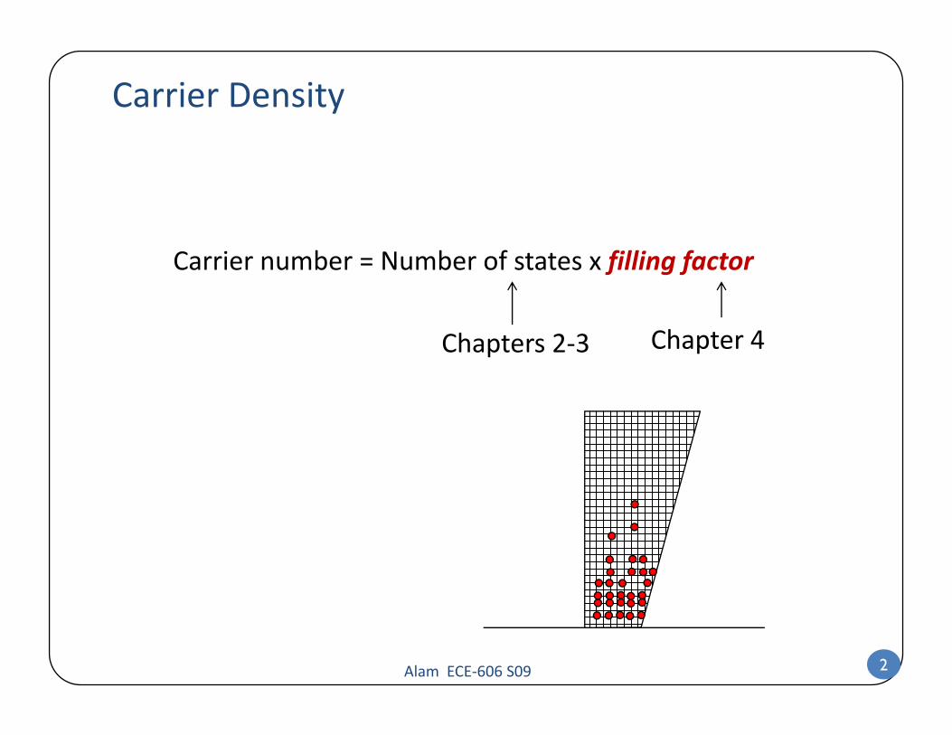
Carrier Density

Carrier number = Number of states x filling factor

Chapters 2‐3 Chapter 4


Outline

1) Rules of filling electronic states1) Rules of filling electronic states

2) Derivation of Fermi‐Dirac Statistics: three techniques

)3) Intrinsic carrier concentration

4) Conclusion

Reference: Vol 6 Ch 4 (pages 96‐105)


Reference: Vol. 6, Ch. 4 (pages 96 105)

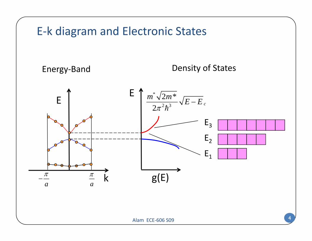
E‐k diagram and Electronic States

Energy‐Band Density of States

EE

2 3

22

−*

cm m* E E2 32π

E

E3

E1

E2

kaπ

aπ

− g(E)


Rules for filling up the States

E3E2

3

E11

Pauli Principle: Only one electron per state

Total number of electrons is conserved T iiN N=∑

Total energy of the system is conserved

T ii∑T i ii

E E N=∑


Outline

1) R l f l i l t i t t1) Rules of placing electronic states


3) Intrinsic carrier concentration

4) Conclusion

In 1926, Fowler studied collapse of a star to white dwarf by F‐D statistics, before Sommerfeld used the F‐D statistics to develop a theory of


electrons in metals in 1927. Wikipedia has a nice article on this topic.

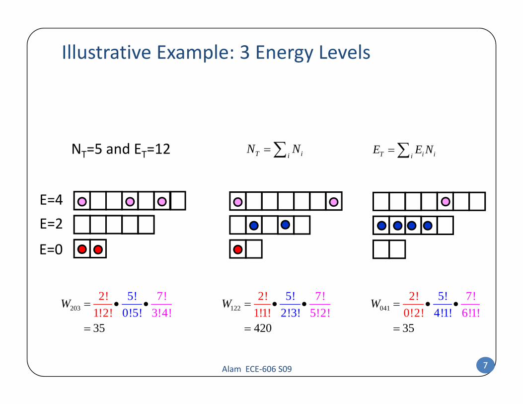
Illustrative Example: 3 Energy Levels

T iiN N=∑ T i ii

E E N=∑NT=5 and ET=12

E=2

E=4

E=0

E 2

2035!

0!5!2!

1!27!

3!5

4!3

!W = • •

=

1225!

2!3!72!

1!1!

5!2!!420

W = • •

=

0415!

4!1!2!

0!27!

6!5

1!3

!W = • •

=


53= 420= 53=

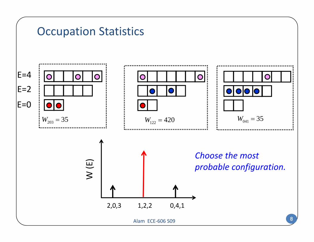
Occupation Statistics

E=4

E=0

E=2

E=4

E=0

122 420W = 041 35W =203 35W =

(E) Choose the most

probable configuration

W ( probable configuration.


2,0,3 1,2,2 0,4,1

Occupation Statistics

E=4 * 2f = E

E=0

E=2

E=4 3

*2

725

f

f

=

=

E

E=0

122 420W =*

1 21f =

f(E)

(E)

W (


2,0,3 1,2,2 0,4,1

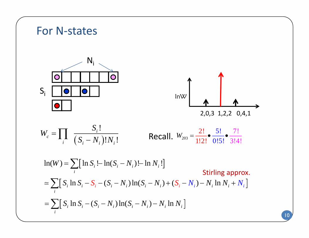
For N‐states

Ni

lnWSi

!iSW =∏

2,0,3 1,2,2 0,4,1

5!2! 7!WR ll( )! !ci i i i

WS N N

=−∏ 203 0!51 ! 3!4!!2!

= • •WRecall.

[ ]ln( ) ln ! ln( )! ln != − − −∑W S S N N

[ ]ln ( ) ln( ) ( ) ln− − − − + − − +∑ i i i i i i i ii i i ii

NS S S N N NS NS N SStirling approx.

[ ]ln( ) ln ! ln( )! ln !=∑ i i i ii

W S S N N

10

[ ]ln ( ) ln( ) ln= − − − −∑ i i i i i i i ii

S S S N S N N N

Optimization with Lagrange‐Multiplierh hChoose the most

probable configuration.

lnWlnln( ) ii i

WW dNN

δ ∂=

∂∑configurations

i

ln 1ii i i i

S dN dN E dNN

α β⎡ ⎤⎛ ⎞

− − −⎢ ⎥⎜ ⎟⎢ ⎥⎝ ⎠⎣ ⎦

∑ ∑ ∑

l 1iS E dNβ⎡ ⎤⎛ ⎞⎢ ⎥⎜ ⎟∑

T i iiE E N=∑

i i iiN⎢ ⎥⎝ ⎠⎣ ⎦∑ ∑ ∑

ln 1ii i

i i

S E dNN

α β⎛ ⎞

= − − −⎢ ⎥⎜ ⎟⎢ ⎥⎝ ⎠⎣ ⎦

∑T ii

N N=∑

i∑


i

Final steps …

ln 1 0ii

S EN

α β⎡ ⎤⎛ ⎞

− − − =⎢ ⎥⎜ ⎟⎢ ⎥⎝ ⎠ E

1iN

iiN

β⎢ ⎥⎜ ⎟⎢ ⎥⎝ ⎠⎣ ⎦

E

EF1( )1 α β+≡ =+

iE

i

Nf ES e

1f(E)

fmax(E)=1EF

1At , ( ) 02FF FE f EE Eα β= ≡ ⇒ + =

1( ) iNf E1

1β

( )1( )

1 F

iE

iE

Nf ES eβ −

= =+

/A ( ) E k Tf A

( ) /1 BFE kE Te −=

+


Bk Tβ⇒ =/At , ( ) BE k T

BoltzmanE f E Ae−→ ∞ =

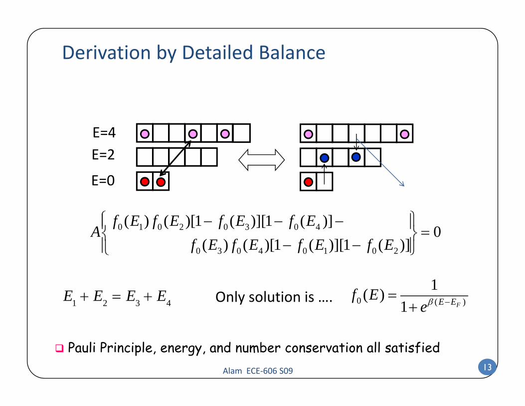
Derivation by Detailed Balance

E 0

E=2E=4

0 1 0 2 0 3 0 4( ) ( )[1 ( )][1 ( )]0

f E f E f E f EA⎧ ⎫− − −⎪ ⎪⎨ ⎬

E=0

0 1 0 2 0 3 0 4

0 3 0 4 0 1 0 2

( ) ( )[ ( )][ ( )]0

( ) ( )[1 ( )][1 ( )]f f f f

Af E f E f E f E

⎪ ⎪ =⎨ ⎬− −⎪ ⎪⎩ ⎭

1 E1 + E2 = E3 + E4 Only solution is …. 0 ( )

1( )1 β −=+ FE Ef E

e


Pauli Principle, energy, and number conservation all satisfied

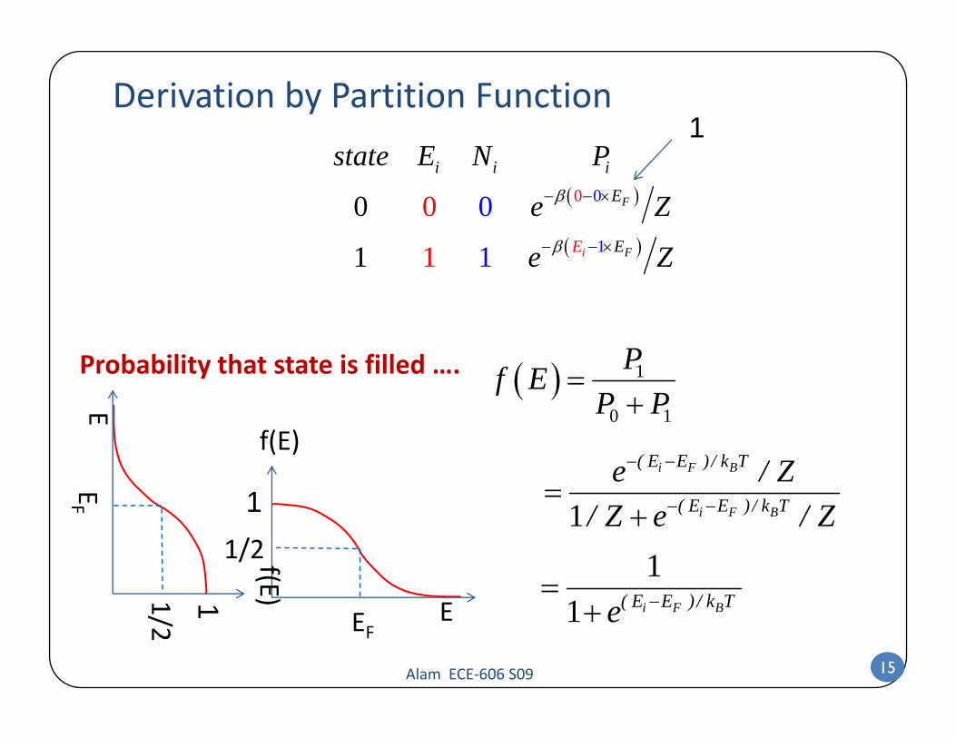
Derivation by Partition Function

β β− − − −F Fiiii( E ) ( E )NE E Ne eP β− −= ≡∑ i i Fi ( E N E )

i

e ePe Z

E=2E=4

E=0 1β = Bk T

( )0000 0 β− − × F

i i i

E

state E N P

e Z( )1

00

11

0

1 β− − ×i FE E

e Z

e ZEi


Derivation by Partition Function1

( )0000 0 β− − × F

i i i

E

state E N P

e Z

1

( )111 1 β− − ×i FE Ee Z

( ) 1

0 1

=+Pf E

P PProbability that state is filled ….

E 0 1

1

− −

− −=i F B

i F B

( E E ) / k T

( E E ) / k T

e / Z/ Z / Z1

f(E)

EF

E

1 + i F B( E E ) / k T/ Z e / Z1

1 −= ( E E ) / k T

11/2f(E)

F


1 −+ i F B( E E ) / k TeEFE

1 )1/2

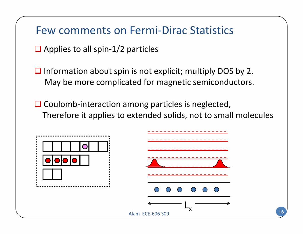
Few comments on Fermi‐Dirac Statistics

Applies to all spin‐1/2 particles

Information about spin is not explicit; multiply DOS by 2Information about spin is not explicit; multiply DOS by 2. May be more complicated for magnetic semiconductors.

C l b i t ti ti l i l t dCoulomb‐interaction among particles is neglected,Therefore it applies to extended solids, not to small molecules

Alam ECE‐606 S09 16Lx

Outline

1) Rules of placing electronic states1) Rules of placing electronic states


3) I i i i i3) Intrinsic carrier concentration

4) Conclusion


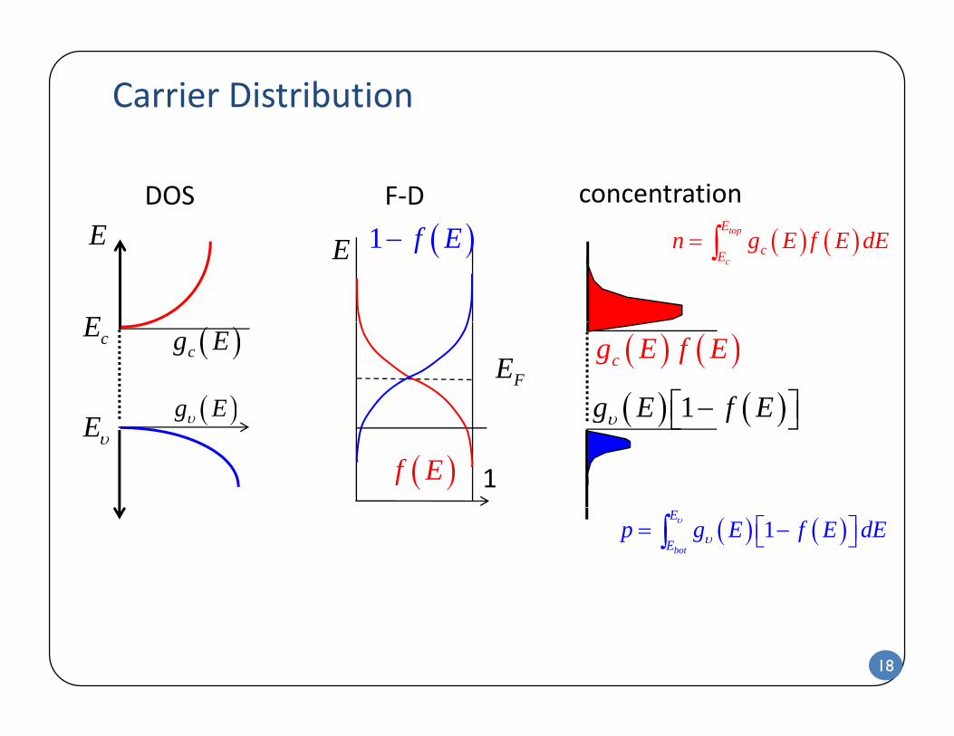
Carrier Distribution

( )1 f E ( ) ( )tE

∫DOS F‐D concentration

E

E

( )1 f E− ( ) ( )top

c

E

cEn g E f E dE= ∫E E

( )cg EFE

( )g E

cE( ) ( )cg E f E

( ) ( )1g E f E⎡ ⎤−⎣ ⎦Eυ( )g Eυ

( )f E

( ) ( )1g E f Eυ ⎡ ⎤⎣ ⎦

1

( ) ( )1bot

E

Ep g E f E dEυ

υ ⎡ ⎤= −⎣ ⎦∫

18

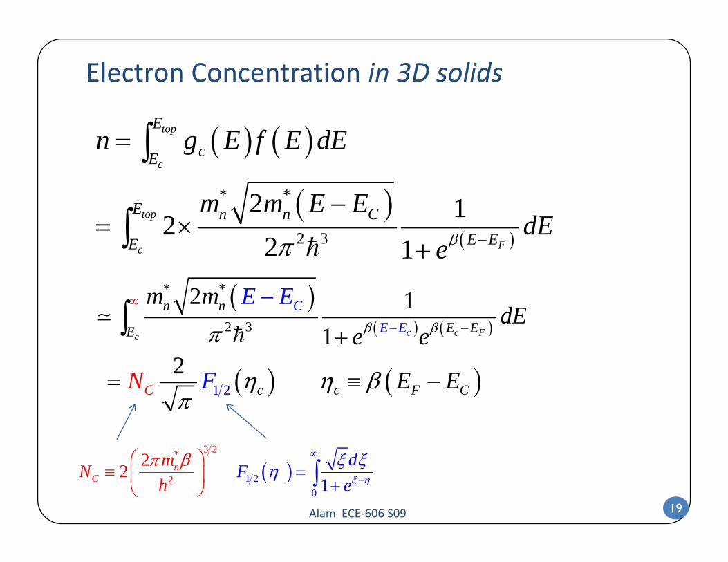
Electron Concentration in 3D solids

( ) ( )= ∫top

c

E

cEn g E f E dE

( )( )2 3

2 122 1 βπ −

−= ×

+∫top

F

* *E n n C

E EE

m m E EdE( )2 1 βπ +∫ FcE e

( )2 1∞ −∫

*Cn

*nm m

dEE E

( ) ( )2 3 1 β βπ − −+∫ c Fc cE E EE E dEe e

( ) ( )1 22 η η β= ≡ −FC CF EN E

3 22 * dmπ β ξ ξ∞⎛ ⎞

( ) ( )1 2 η η βπ c c FC CF EN E


( )2 1 20 1

22 nC

dF

emNh ξ η

π β ξ ξη −=

⎛ ⎞≡ ⎜ ⎟

⎝ ⎠ +∫

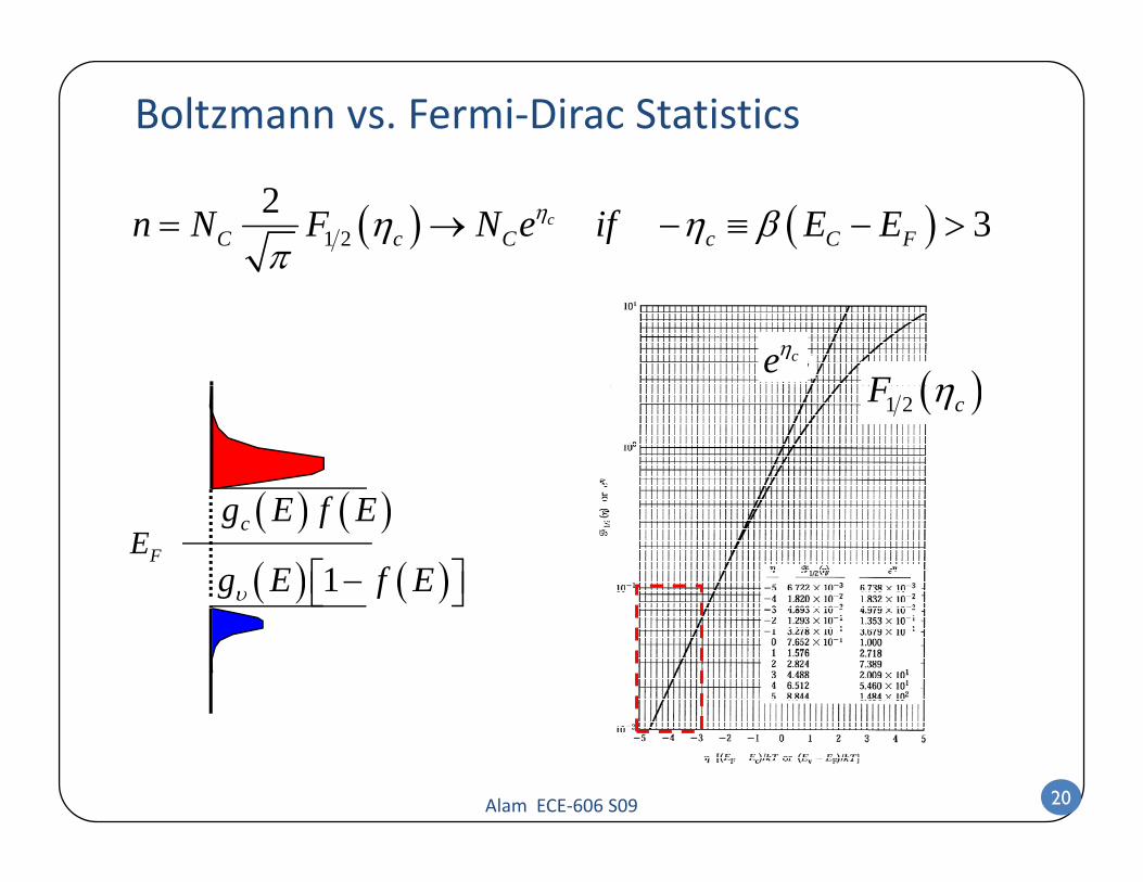
Boltzmann vs. Fermi‐Dirac Statistics

( ) ( )1 22 3ηη η βπ

= → − ≡ − >cC c C c C Fn N F N e if E E

ηce( )ηF

( ) ( )f

( )1 2 ηcF

( ) ( )cg E f E

( ) ( )1g E f Eυ ⎡ ⎤−⎣ ⎦FE


Effective Density of States

( )2 E Eβ( ) ( )1 2

2 3c FE EC c C c Fn N F N e if E Eβη β

π− −= → − >

( ) ( )fCN

( ) ( )cg E f E

( ) ( )1g E f Eυ ⎡ ⎤−⎣ ⎦ VNFE

FE

V

As if all states are at a single level E


As if all states are at a single level EC

Law of Mass‐Action

( )β− −= c FE En N e

( )β+

= C

E E

n N e

( )β+ −= v FE EVp N e

FE

( )β

β

− −× = c vE EC V

E

n p N N eβ−= gE

C VN N e


Fermi‐Level for Intrinsic Semiconductors

2 β

= = i

E

p nn

2βEFE

2 β−= gV

Ei C Nn eN

2β−=

≡

gEi

F

V

i

Cn eE

NE

N≡F iE E

( ) ( )β β− − + −= ⇒ =c i v iE E E En p e eNN E

12 2β

= ⇒ =

= +Gi

V

VCn p e eEE ln

NN

N

N

3


2 2β CNk

2

Conclusions

We discussed how electrons are distributed in electronic states defined by the solution of Schrodinger equationstates defined by the solution of Schrodinger equation.

Since electrons are distributed according to their energy,irrespective of their momentum states, the previously developed concepts of constant energy surfaces, density of states etc. turn out to be very useful.y

We still do not know where EF is for general semiconductors … If we did we could calculate electron concentrationIf we did, we could calculate electron concentration.


Date post:	18-Mar-2022
Category:	Documents
Upload:	others
View:	4 times
Download:	0 times

EE-606: Solid State Devices Lecture 9: Fermi-Dirac - nanoHUB

Documents