EE365 and MS&E251: Introduction

About the course

Optimization

Dynamical systems

Stochastic control

1

About the course

2

About the course

I EE365 is the same as MS&E251

I created by Stephen Boyd, Sanjay Lall, and Ben Van Roy in 2012

I taught by Sanjay Lall this year

3

Control

I multi-step decision making, in an uncertain dynamic environment

I observe, act, observe, act, . . .

I your current action affects the future

I there is uncertainty in what the effect of your action will be

I goal is to find policy

I (computational) map from what you know to what you do

I called recourse or feedback, a richer concept than optimization

4

Applications

I multi-period investment

I automatic control

I supply chain optimization

I internet ad display

I revenue management

I operation of a smart grid

I data center operation

. . . and many, many others. What is the common abstraction?

5

Approach

I how to formulate and solve problems

I solution is usually an algorithm

I focus on ideas, not technicalities of corner cases

I similar style to ee263

I practical homeworks with extensive coding

I Matlab, not Julia, Python, . . .

6

Dynamics

intellectual components

I observe: statistical inference

I decide: optimization

I repeat: dynamics, with uncertainty

this course focuses on the consequences of dynamics, specifically:

I dynamic programming

I for Markov decision processes

7

Prerequisites

I linear algebra (EE263 or MS&E211; more than Math 51)

I probability (EE178/278A or MS&E220)

I not dependencies, but may increase appreciation:

I other classes in control

I artificial intelligence, Markov chains, optimization

8

Curriculum

I MS&E251 in the MS core, and in decision and risk analysis

I EE&365 satisfies MS breadth, and in two depth sequences:

I control and system engineering

I dynamical systems and optimization

9

Administration

I TAs: Samuel Bakouch and Alex Lemon

I the website ee365.stanford.edu

I piazza, coursework

I you have some grace days for homework

I 70% final, 30% homework

I 24-hour take-home final exam, only 6/6, 6/7, 6/8, 6/9, 6/10 or 6/11

10

Books

I Puterman, Markov Decision Processes: Discrete Stochastic Dynamic Pro-gramming (online)

I Bertsekas, Dynamic Programming and Optimal Control, vol. 1

11

Optimization

12

Optimization problem

minimize f(x)subject to x ∈ X

I x is decision variable (discrete, continuous)

I X is constraint set

I f : X → R is objective (cost function)

I x is feasible if x ∈ X

I x is optimal (or a solution) if f(x) = infz∈X f(z)

I f and X can depend on parameters (data)

I can maximize by minimizing −f (reward, utility, profit, . . . )

I standard trick: allow f(x) =∞ (to embed further constraints in objective)

13

Solving optimization problems

I a solution method or algorithm computes a solution, given parameters

I difficulty of solving optimization problem depends on

I mathematical properties of f , XI problem size (e.g., dimension of x when x ∈ Rn)

I a few problems can be solved ‘analytically’

I but this is not particularly relevant, since we adopt algorithmic approach

14

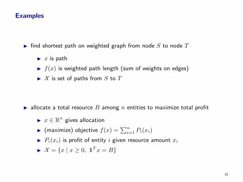
Examples

I find shortest path on weighted graph from node S to node T

I x is path

I f(x) is weighted path length (sum of weights on edges)

I X is set of paths from S to T

I allocate a total resource B among n entities to maximize total profit

I x ∈ Rn gives allocation

I (maximize) objective f(x) =∑n

i=1 Pi(xi)

I Pi(xi) is profit of entity i given resource amount xi

I X = {x | x ≥ 0, 1Tx = B}

15

Dynamical systems

16

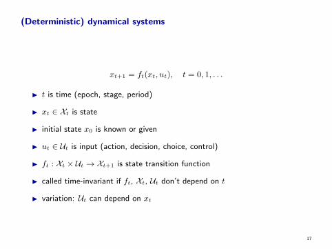
(Deterministic) dynamical systems

xt+1 = ft(xt, ut), t = 0, 1, . . .

I t is time (epoch, stage, period)

I xt ∈ Xt is state

I initial state x0 is known or given

I ut ∈ Ut is input (action, decision, choice, control)

I ft : Xt × Ut → Xt+1 is state transition function

I called time-invariant if ft, Xt, Ut don’t depend on t

I variation: Ut can depend on xt

17

Idea of state

I current action affects future states, but not current or past states

I current state depends on past actions

I state is link between past and future

I if you know state xt and actions ut, . . . , us−1, you know xs

I u0, . . . , ut−1 not relevant

I state is sufficient statistic (summary) for past

18

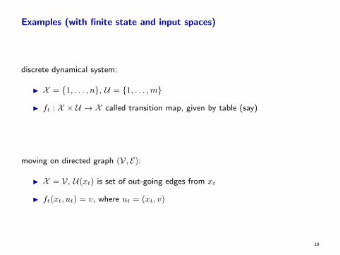
Examples (with finite state and input spaces)

discrete dynamical system:

I X = {1, . . . , n}, U = {1, . . . ,m}

I ft : X × U → X called transition map, given by table (say)

moving on directed graph (V, E):

I X = V, U(xt) is set of out-going edges from xt

I ft(xt, ut) = v, where ut = (xt, v)

19

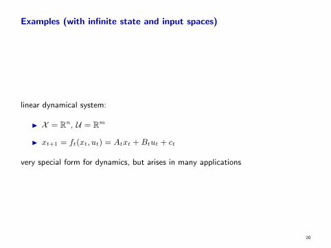
Examples (with infinite state and input spaces)

linear dynamical system:

I X = Rn, U = Rm

I xt+1 = ft(xt, ut) = Atxt +Btut + ct

very special form for dynamics, but arises in many applications

20

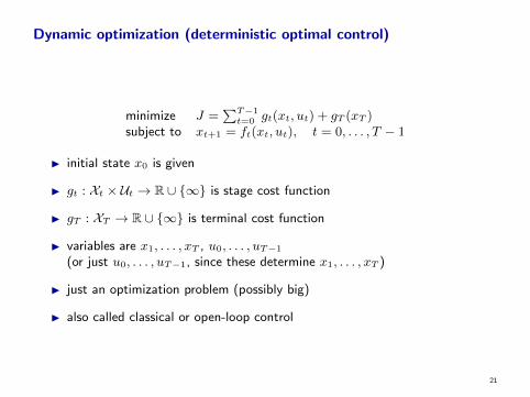
Dynamic optimization (deterministic optimal control)

minimize J =∑T−1

t=0 gt(xt, ut) + gT (xT )subject to xt+1 = ft(xt, ut), t = 0, . . . , T − 1

I initial state x0 is given

I gt : Xt × Ut → R ∪ {∞} is stage cost function

I gT : XT → R ∪ {∞} is terminal cost function

I variables are x1, . . . , xT , u0, . . . , uT−1

(or just u0, . . . , uT−1, since these determine x1, . . . , xT )

I just an optimization problem (possibly big)

I also called classical or open-loop control

21

Deterministic optimal control

I addresses dynamic effect of actions across time

I no uncertainty or randomness in model

I is widely used (often, by simply ignoring uncertainty in the application)

22

Stochastic control

23

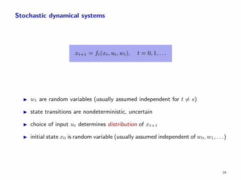
Stochastic dynamical systems

xt+1 = ft(xt, ut, wt), t = 0, 1, . . .

I wt are random variables (usually assumed independent for t 6= s)

I state transitions are nondeterministic, uncertain

I choice of input ut determines distribution of xt+1

I initial state x0 is random variable (usually assumed independent of w0, w1, . . .)

24

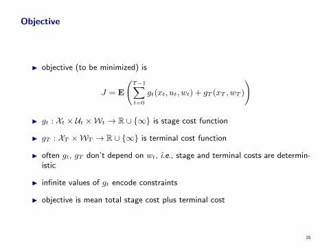
Objective

I objective (to be minimized) is

J = E

(T−1∑t=0

gt(xt, ut, wt) + gT (xT , wT )

)

I gt : Xt × Ut ×Wt → R ∪ {∞} is stage cost function

I gT : XT ×WT → R ∪ {∞} is terminal cost function

I often gt, gT don’t depend on wt, i.e., stage and terminal costs are determin-istic

I infinite values of gt encode constraints

I objective is mean total stage cost plus terminal cost

25

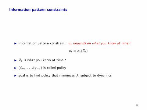
Information pattern constraints

I information pattern constraint: ut depends on what you know at time t

ut = φt(Zt)

I Zt is what you know at time t

I (φ0, . . . , φT−1) is called policy

I goal is to find policy that minimizes J , subject to dynamics

26

Information patterns

I full knowledge (prescient): Zt = (w0, . . . , wT−1)

I for each realization, reduces to deterministic optimal control problem

I no knowledge: Zt = ∅

I reduces to an optimization problem; called open-loop

I in between: Zt = xt (called state feedback)

I a little more: Zt = (xt, wt)

these are very different problems!

27

Example: Stochastic shortest path

I move from node S to node T in directed weighted graph

I minimize expected total weight along path

I edge weights are random variables, independent in each time period

information patterns:

I no knowledge: commit to path beforehand(knowing distributions of weights, but not actual values)

I full knowledge: weights on all edges at all times are revealed before path ischosen

I local knowledge: at each node, at each time, weights of out-going edges arerevealed before next edge on path is chosen

28

Example: Optimal disposition of stock

I sell a total amount S of a stock in T periods

I price (and transaction cost) varies randomly

I maximize expected revenue

information patterns:

I no knowledge: commit to sales amounts beforehand

I in each time period, the price and transaction cost is known before amountsold is chosen

29