Lehrstuhl f¨ ur Entwurfsautomatisierung der Technischen Universit¨ at M ¨ unchen Efficient Quadratic Placement of VLSI Circuits Peter Spindler Vollst¨ andiger Abdruck der von der Fakult¨ at f¨ ur Elektrotechnik und Informationstechnik der Technischen Universit¨ at M ¨ unchen zur Erlangung des akademischen Grades eines Doktor-Ingenieurs genehmigten Dissertation. Vorsitzender: Univ.-Prof. Dr. techn. Josef A. Nossek Pr¨ ufer der Dissertation: 1. Univ.-Prof. Dr.-Ing. Frank M. Johannes 2. Univ.-Prof. Dr.-Ing. Jens Lienig Technische Universit¨ at Dresden Die Dissertation wurde am 20.12.2007 bei der Technischen Universit¨ at M ¨ unchen eingereicht und durch die Fakult¨ at f¨ ur Elektrotechnik und Informationstechnik am 05.06.2008 angenom- men.
Vollstandiger Abdruck der von der Fakultat fur Elektrotechnik und Informationstechnik derTechnischen Universitat Munchen zur Erlangung des akademischen Grades eines
Doktor-Ingenieurs
genehmigten Dissertation.
Vorsitzender: Univ.-Prof. Dr. techn. Josef A. Nossek
Prufer der Dissertation:
1. Univ.-Prof. Dr.-Ing. Frank M. Johannes2. Univ.-Prof. Dr.-Ing. Jens Lienig
Technische Universitat Dresden
Die Dissertation wurde am 20.12.2007 bei der Technischen Universitat Munchen eingereichtund durch die Fakultat fur Elektrotechnik und Informationstechnik am 05.06.2008 angenom-men.
Acknowledgment
This thesis is the result of my work and all the help and advicethat has been provided tome through all of my years at the Institute for Electronic Design Automation, TechnischeUniversitat Munchen, Germany.
The person who deserves most of my credit is undoubtedly my adviser Professor FrankM. Johannes. With the prolific discussions, not only about the field of research, and hiscontinuous encouragement, he gave the essential requirements for successful research. I amalso very grateful for the constant support and inspirationof Professor Ulf Schlichtmann. Iwould also like to thank Professor Jens Lienig and ProfessorJosef A. Nossek for their interestin my thesis and their job as reviewers.
The many interesting discussions with my colleagues contributed much to this thesis.Amongst others, I would like to thank Martin Strasser, Dr. Helmut Grab, and my predecessorin the layout group, Dr. Bernd Obermeier. Special thanks go to Dr. Hans Eisenmann, who laidwith his work the basis for this thesis. I owe respect to Dr. Bernd Finkbein, Getraude Kall-weit, Hans Ranke, Werner Tolle, Susanne Werner, and JurgenZenz for their administrativeand technical support.
Finally, I would like to thank with all my heart my girlfriendKatrin Mayer-Arnold, whoalways stands behind me and supports me under all circumstances.
Integrated circuits (ICs) are part of our daily live as they are the hearts of MP3 players, cellphones, personal digital assistants (PDAs), laptops, and even cars have a high number ofintegrated circuits. Also the industry mainly depends on integrated circuits in different appli-cations, ranging from simulations of complex processes on main-frame computers to efficientcontrol of production lines.
The history of integrated circuits started around 1960, when analog components wereintegrated on a piece of silicon for the first time. In 1971, Intel presented the 4004, the firstmicroprocessor of the world with about 2300 transistors. Atthe time this thesis was written,integrated circuits can have billions of transistors. Hence, integrated circuits are today mostlycalled VLSI circuits, with VLSI standing for very large scale integration. This enormouscomplexity of integrated circuits can only be handled if thecircuits are designed not by hand,but by algorithms, executed on computers. The usage of such computer algorithms in orderto design integrated circuits is called electronic design automation (EDA).
In the year 1965, Gordon Moore [Moo65] detected that the numbers of transistors inan integrated circuit is doubling every 18 months (approximately). Still today, Moore’s lawis valid [SEM], which means that the complexity of integrated circuit is steadily growing.Therefore, fast and efficient algorithms are necessary for the EDA of future circuits.
1.1 Electronic Design Automation
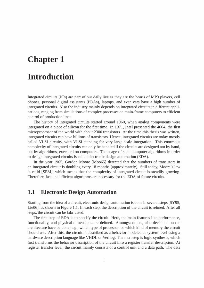
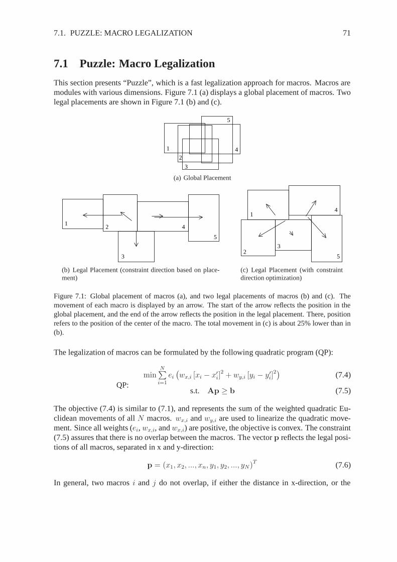
Starting from the idea of a circuit, electronic design automation is done in several steps [SY95,Lie06], as shown in Figure 1.1. In each step, the descriptionof the circuit is refined. After allsteps, the circuit can be fabricated.
The first step of EDA is to specify the circuit. Here, the main features like performance,functionality, and physical dimensions are defined. Amongst others, also decisions on thearchitecture have be done, e.g., which type of processor, orwhich kind of memory the circuitshould use. After this, the circuit is described as a behavior modeled at system level using ahardware description language like VHDL or Verilog. The next step is logic synthesis, whichfirst transforms the behavior description of the circuit into a register transfer description. Atregister transfer level, the circuit mainly consists of a control unit and a data path. The data
1
2 CHAPTER 1. INTRODUCTION
&&
≥1
&
=1≥1
Final Placement
Routing
Global Placement
Specification
Logic Synthesis
Simulation/Verification
Layou
tSyn
thesis
Polygone Level
Gate Level
System Level
Th
isT
hes
is
Simulation/Verification
Idea
Fabrication
wait until clock’event and clock=’1’
variable x,y,u,x1,y1,u1: fixpnt := 0;
wait until start’event and start=’1’;
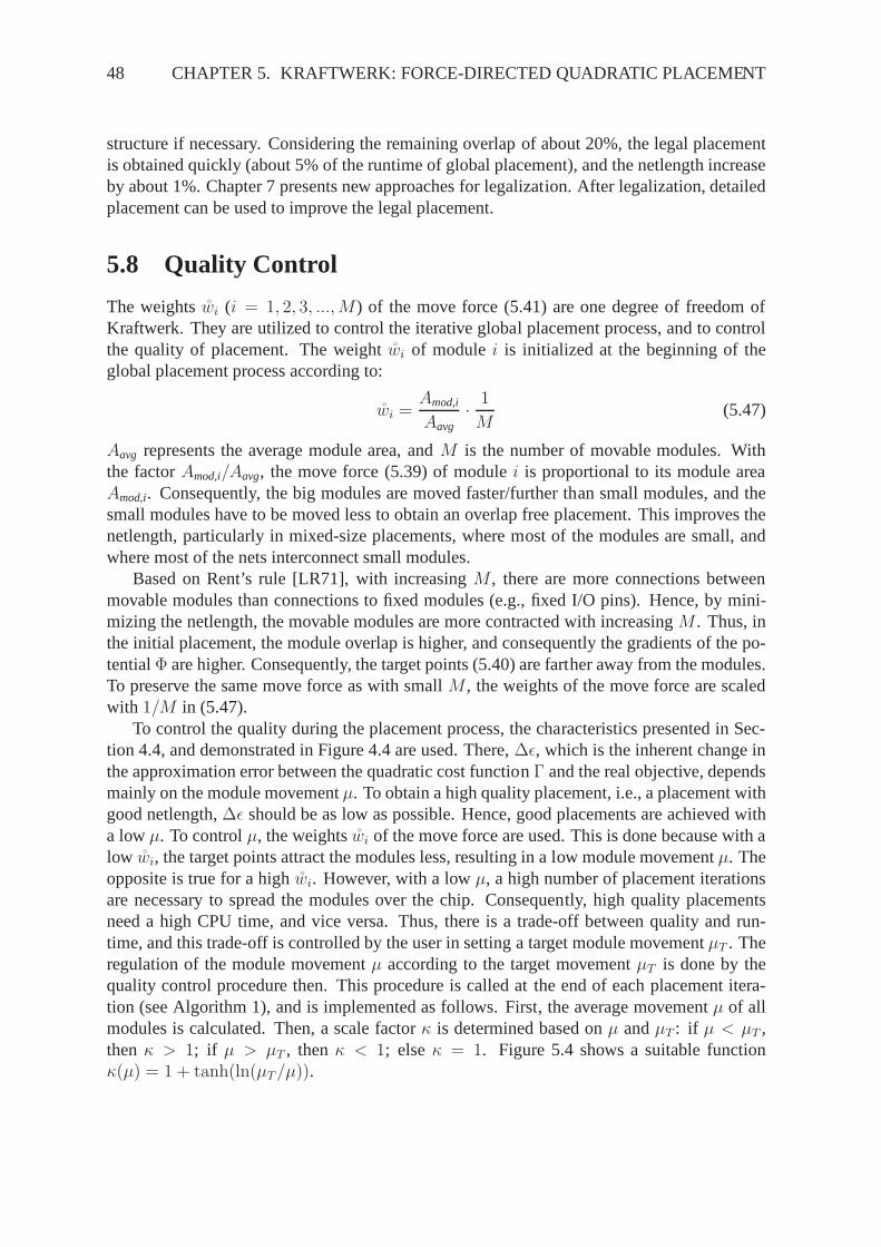
architecture BEHAVIOR of DIFFEQ isbeginprocess
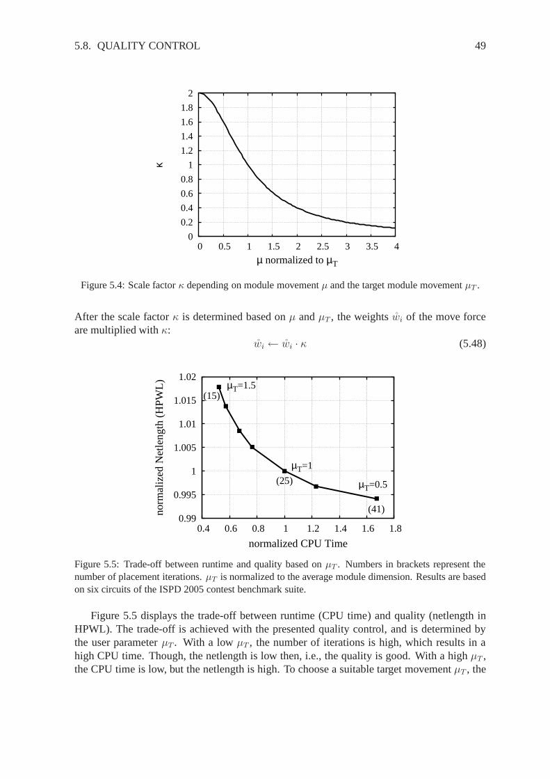
variable c: bit := false;
x:=x0; y:=y0; u:=u0;loop
x1:=x+dx;y1:=y+u*dx;
begin
u1:=u-3*x*u*dy - 3*y*dx;c:=x1 < xe;
x:=x1; y:=y1; u:=u1;end loop;y out <= y;
end process;end BEHAVIOR;
exit when not c
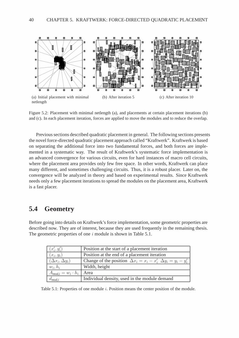
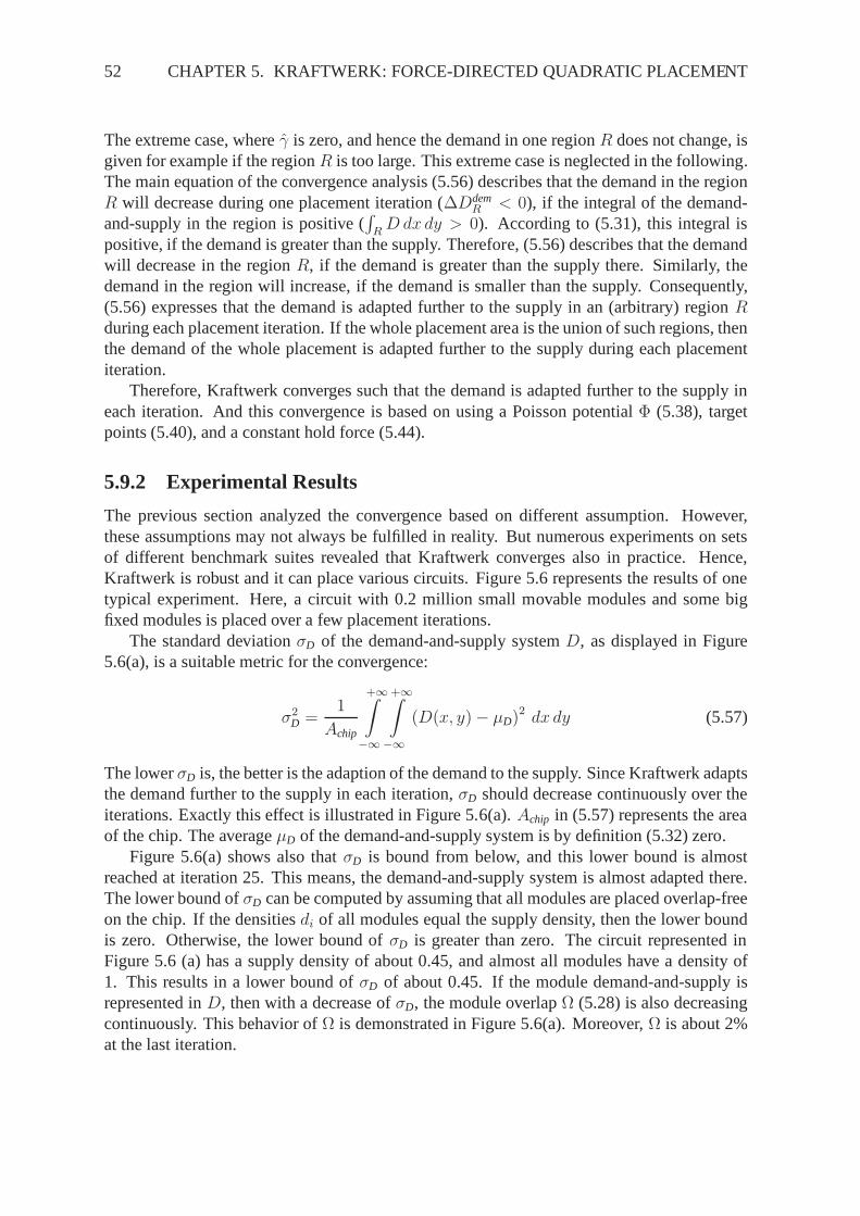
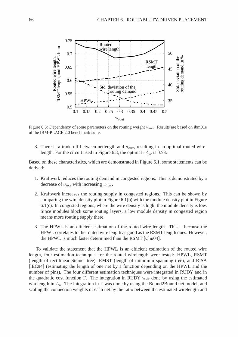
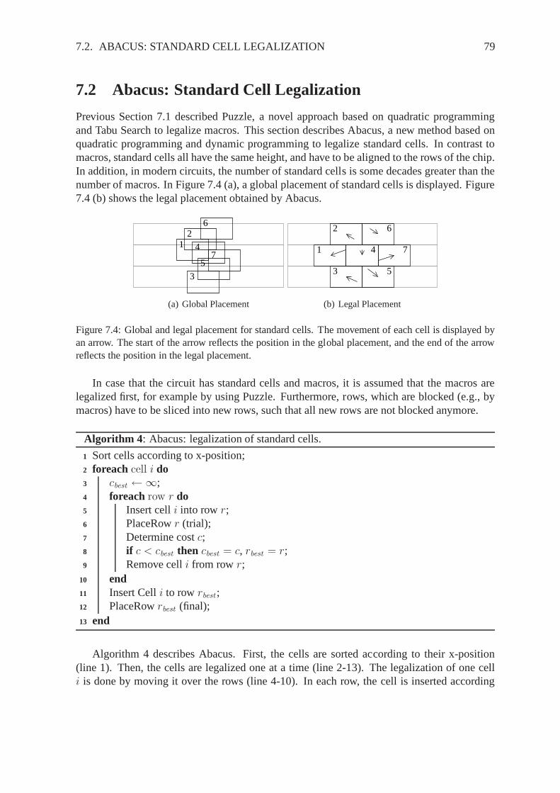
Figure 1.1: Design Flow of Integrated Circuits
1.2. TYPES OF INTEGRATED CIRCUITS 3
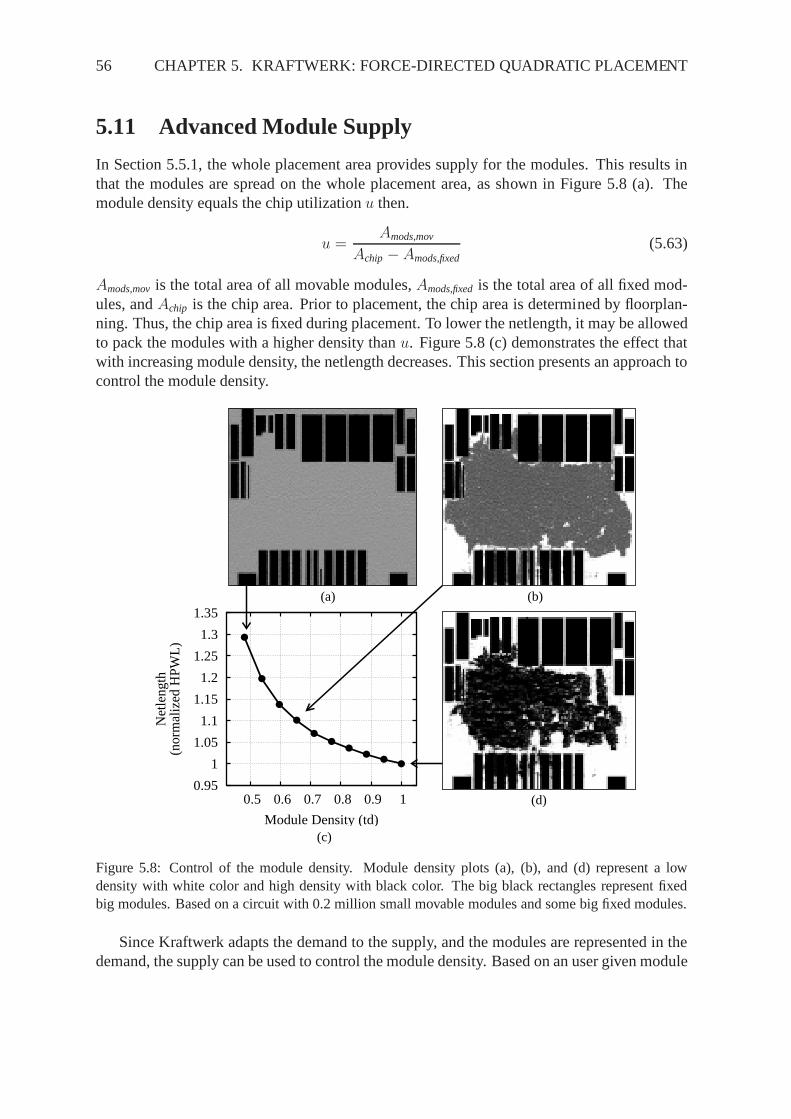
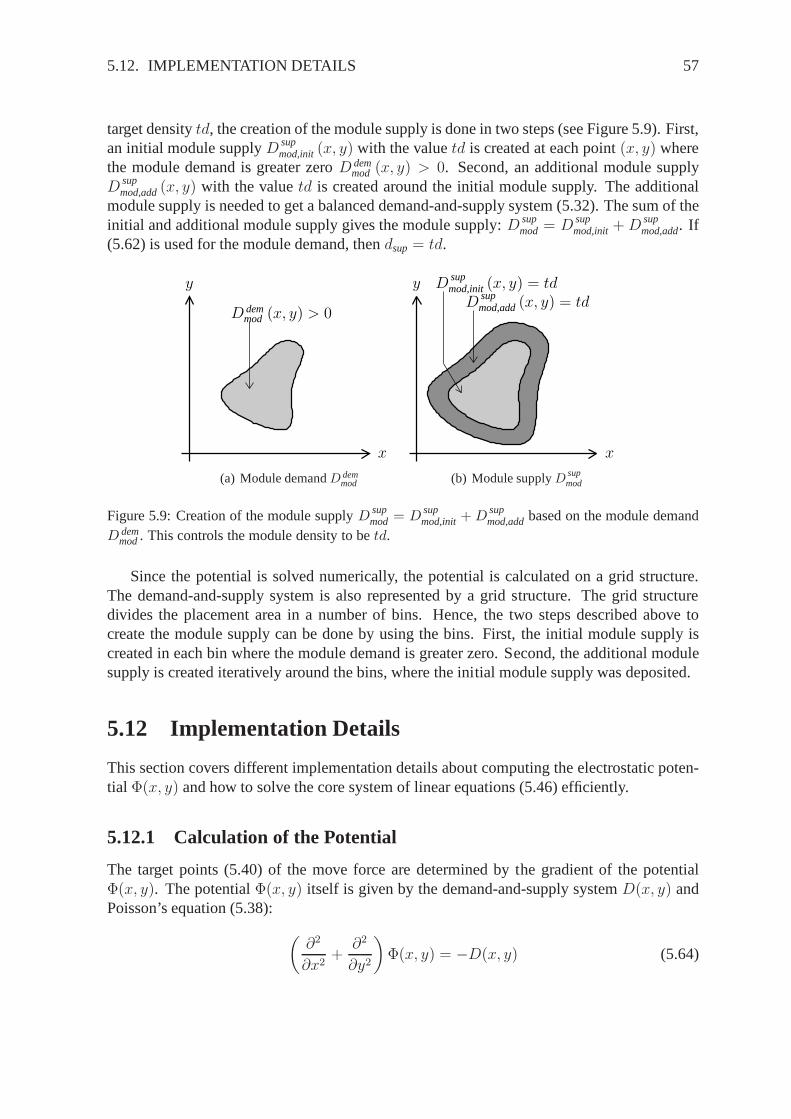
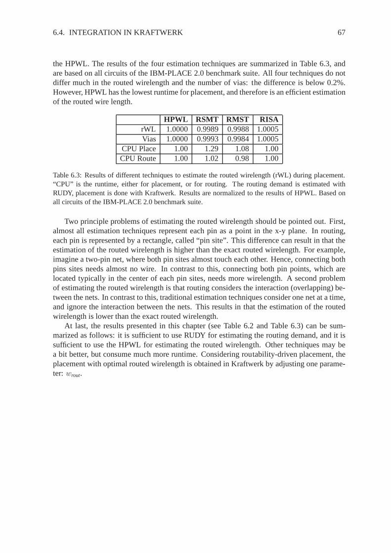
path includes registers and functional blocks like arithmetic logic units. Moreover, the data aredescribed as bit vectors. Based on the register transfer model of the circuit, the logic synthesisconstructs the gate level description then. At gate level, the circuit consists of gates likeinverters, and-gates, or-gates, flip-flops, etc. The gates themselves consists of transistors. Thedata are described as single bits. After logic synthesis, the gate level description of the circuitis simulated, and different specifications are verified, e.g., the maximal clock frequency. If thespecifications are not met, the logic synthesis is done again. If the circuit is working correctlyat gate-level, layout synthesis is done next. The main stepsof layout synthesis is placement ofthe gates, and routing of the nets, which interconnect the gates. However, prior to placement,floorplanning is invoked to determine the positions of the I/O pins, the dimensions of biggates, and the dimensions of the chip. Due to the high numbersof gates, placement itselfis done in two steps: global placement and final placement. During global placement, thegates are roughly spread on the chip. Final placement then removes the remaining overlap,aligns the gates to a given row/grid structure. There, different design rules are considered,like minimal distances between the gates. This thesis presents novel approaches for globaland final placement. After the gates are placed, the nets, which interconnect the gates, arerouted. After routing, the polygon level of the circuit is reached, i.e., the circuit is describedonly by polygons now. At polygon level, the circuit is simulated again, and it is checked if allgiven specifications are met. If not, the EDA is started from previous steps, and if necessary,it is even started again with logic synthesis. At the end of EDA, the lithography masks arecreated, and the circuit is fabricated using these masks.
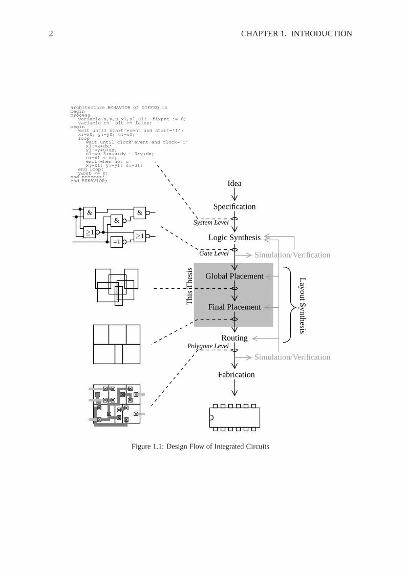
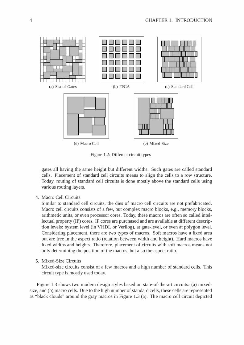
1.2 Types of Integrated Circuits
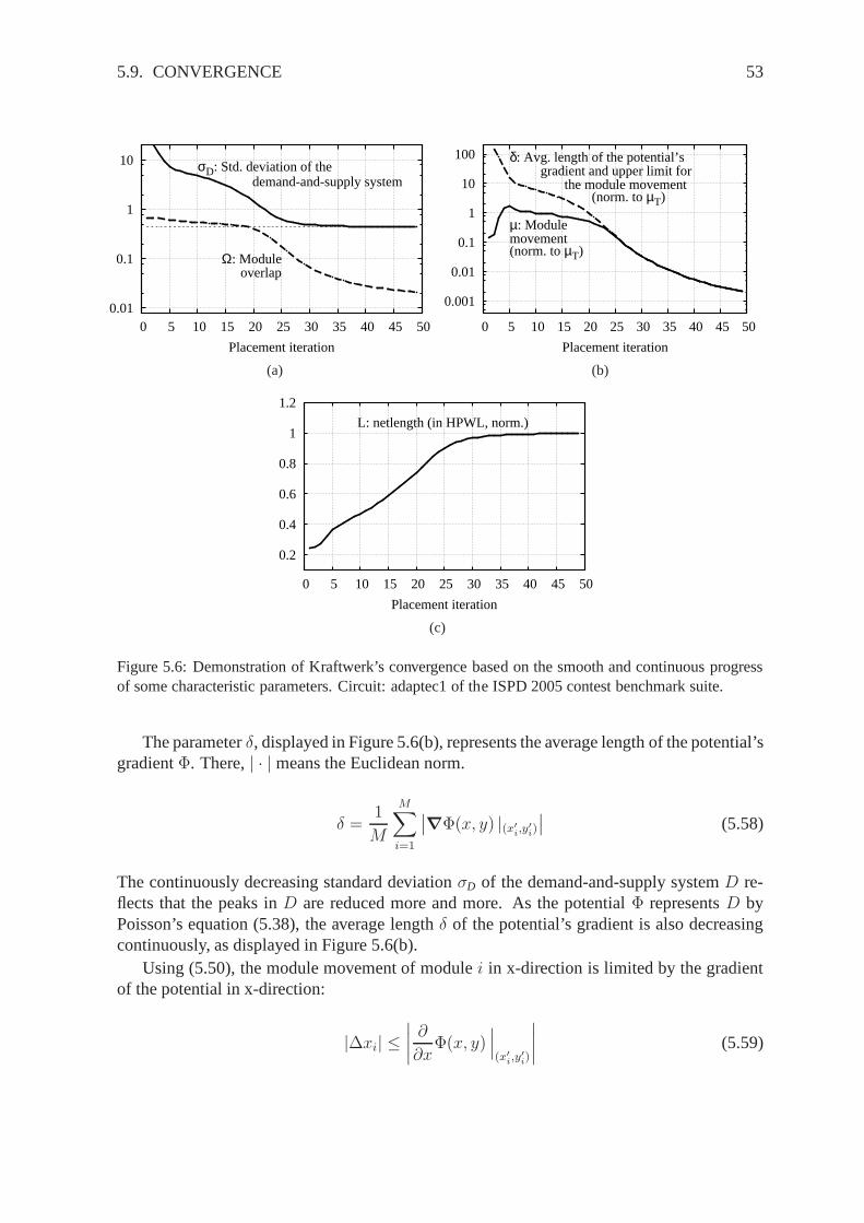
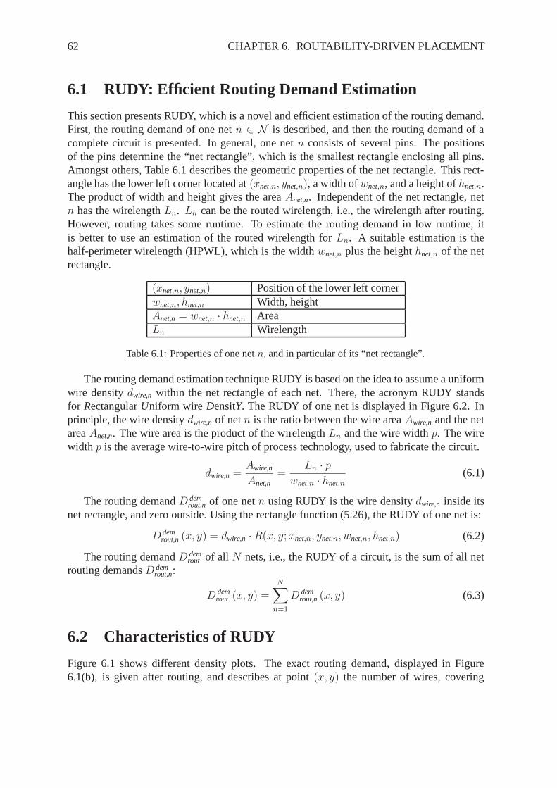
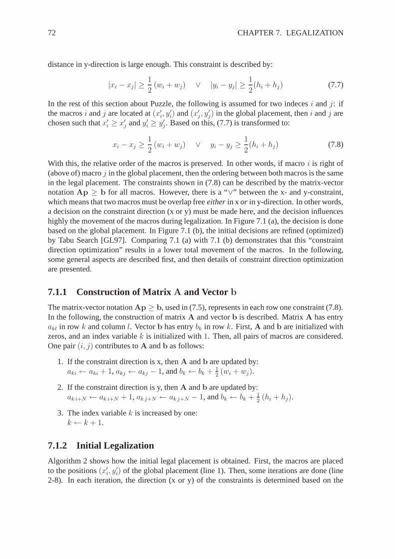
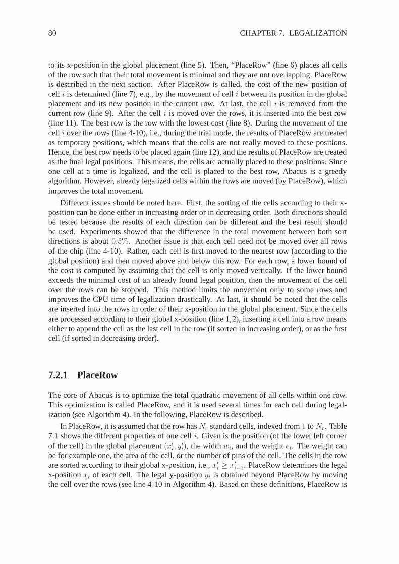
Figure 1.2 displays different types of integrated circuitsused today. Each circuit type reflectone design style. The differences between them is mainly thetype of gates, and how theyare implemented on the “die”. “Die” here means the piece of silicon which implements thecircuit.
1. Mask-Programmable Gate-Arrays/Sea-of-GatesThe dies of mask-programmable gate-arrays and the dies of sea-of-gates have prefab-ricated transistors, aligned in a regular pattern. To implement circuits with such dies,the gates of the circuit are broken down to transistors first.Then, the gates as groups oftransistors are assigned (placed) to the prefabricated transistors of the die. The routingis done in metal layers, either in channels between the transistors (mask-programmablegate-arrays), or above the transistors (sea-of-gates).
2. Field-Programmable Gate-Arrays (FPGA)The die of a FPGA is completely prefabricated, and consists of a regular matrix of pro-grammable logic blocks and interconnect blocks. Placementof FPGAs means to assigngates of the circuit to the logic blocks of the FPGA. Routing is done by configuring theinterconnect blocks.
3. Standard Cell CircuitsThe die of a standard cell circuit is not prefabricated. The circuit is implemented with
4 CHAPTER 1. INTRODUCTION
(a) Sea-of-Gates (b) FPGA (c) Standard Cell
(d) Macro Cell (e) Mixed-Size
Figure 1.2: Different circuit types
gates all having the same height but different widths. Such gates are called standardcells. Placement of standard cell circuits means to align the cells to a row structure.Today, routing of standard cell circuits is done mostly above the standard cells usingvarious routing layers.
4. Macro Cell CircuitsSimilar to standard cell circuits, the dies of macro cell circuits are not prefabricated.Macro cell circuits consists of a few, but complex macro blocks, e.g., memory blocks,arithmetic units, or even processor cores. Today, these macros are often so called intel-lectual property (IP) cores. IP cores are purchased and are available at different descrip-tion levels: system level (in VHDL or Verilog), at gate-level, or even at polygon level.Considering placement, there are two types of macros. Soft macros have a fixed areabut are free in the aspect ratio (relation between width and height). Hard macros havefixed widths and heights. Therefore, placement of circuits with soft macros means notonly determining the position of the macros, but also the aspect ratio.
5. Mixed-Size CircuitsMixed-size circuits consist of a few macros and a high numberof standard cells. Thiscircuit type is mostly used today.
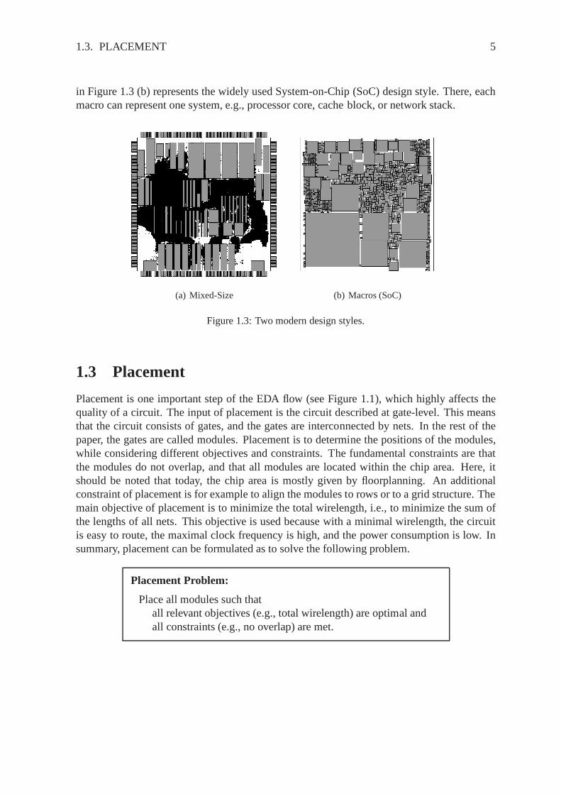
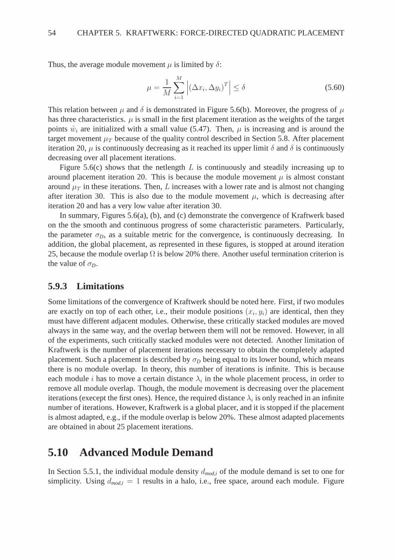
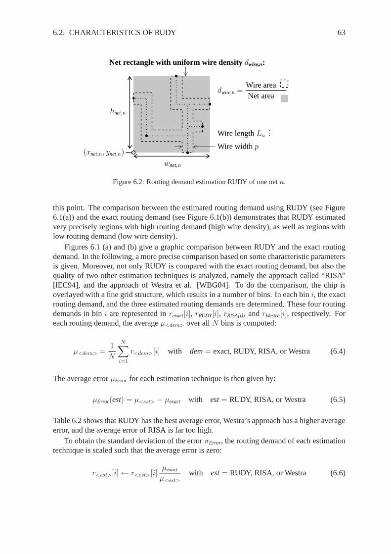
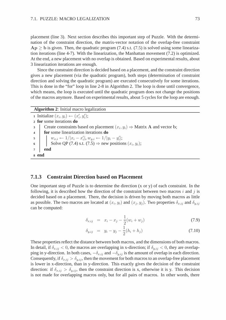
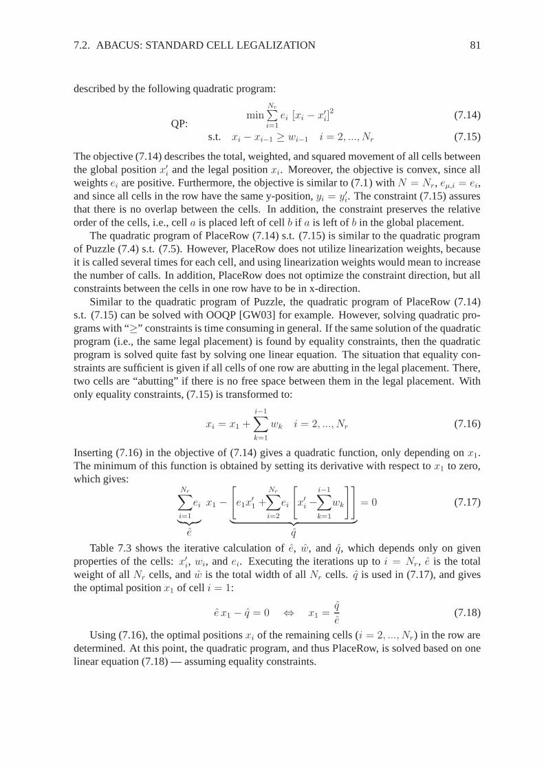
Figure 1.3 shows two modern design styles based on state-of-the-art circuits: (a) mixed-size, and (b) macro cells. Due to the high number of standard cells, these cells are representedas “black clouds” around the gray macros in Figure 1.3 (a). The macro cell circuit depicted
1.3. PLACEMENT 5
in Figure 1.3 (b) represents the widely used System-on-Chip(SoC) design style. There, eachmacro can represent one system, e.g., processor core, cacheblock, or network stack.
(a) Mixed-Size (b) Macros (SoC)
Figure 1.3: Two modern design styles.
1.3 Placement
Placement is one important step of the EDA flow (see Figure 1.1), which highly affects thequality of a circuit. The input of placement is the circuit described at gate-level. This meansthat the circuit consists of gates, and the gates are interconnected by nets. In the rest of thepaper, the gates are called modules. Placement is to determine the positions of the modules,while considering different objectives and constraints. The fundamental constraints are thatthe modules do not overlap, and that all modules are located within the chip area. Here, itshould be noted that today, the chip area is mostly given by floorplanning. An additionalconstraint of placement is for example to align the modules to rows or to a grid structure. Themain objective of placement is to minimize the total wirelength, i.e., to minimize the sum ofthe lengths of all nets. This objective is used because with aminimal wirelength, the circuitis easy to route, the maximal clock frequency is high, and thepower consumption is low. Insummary, placement can be formulated as to solve the following problem.
Placement Problem:
Place all modules such thatall relevant objectives (e.g., total wirelength) are optimal andall constraints (e.g., no overlap) are met.
6 CHAPTER 1. INTRODUCTION
Chapter 2
State of the Art
Although the placement problem proposed in the previous section sounds easy, it is a combi-natorial problem, which is known to be a NP-complete problem[GJ79, Don80, SB80, Len88,Len90]. This means, there exists no algorithm up to date, which solves the problem optimalwith polynomial runtime complexity. In the extreme case, all feasible placements have tobe inspected, in order to find the optimal placement. With millions of modules (which is thenumber of modules in modern VLSI circuits), the number of feasible placements is quite high,i.e., the runtime is not practicable.
Hence, to get good solutions in polynomial runtime, the placement problem is solved byheuristics. One traditional method is to use two steps for placement: global and final place-ment. In global placement, the modules are spread roughly onthe chip, with few overlapremaining. In final placement, the overlap is removed, and the modules are aligned to thegrid/row structure. This thesis covers novel solutions forboth placement steps. In the fol-lowing, the state-of-the-art in global placement is described first, including different aspectsas net models and routability optimization. Second, the state-of-the-art in final placement ispresented.
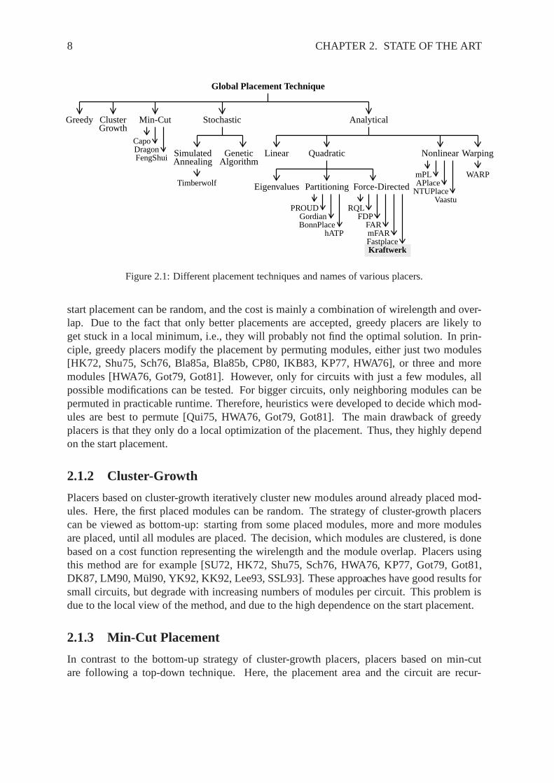
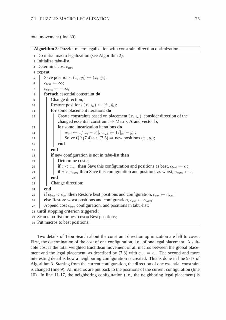
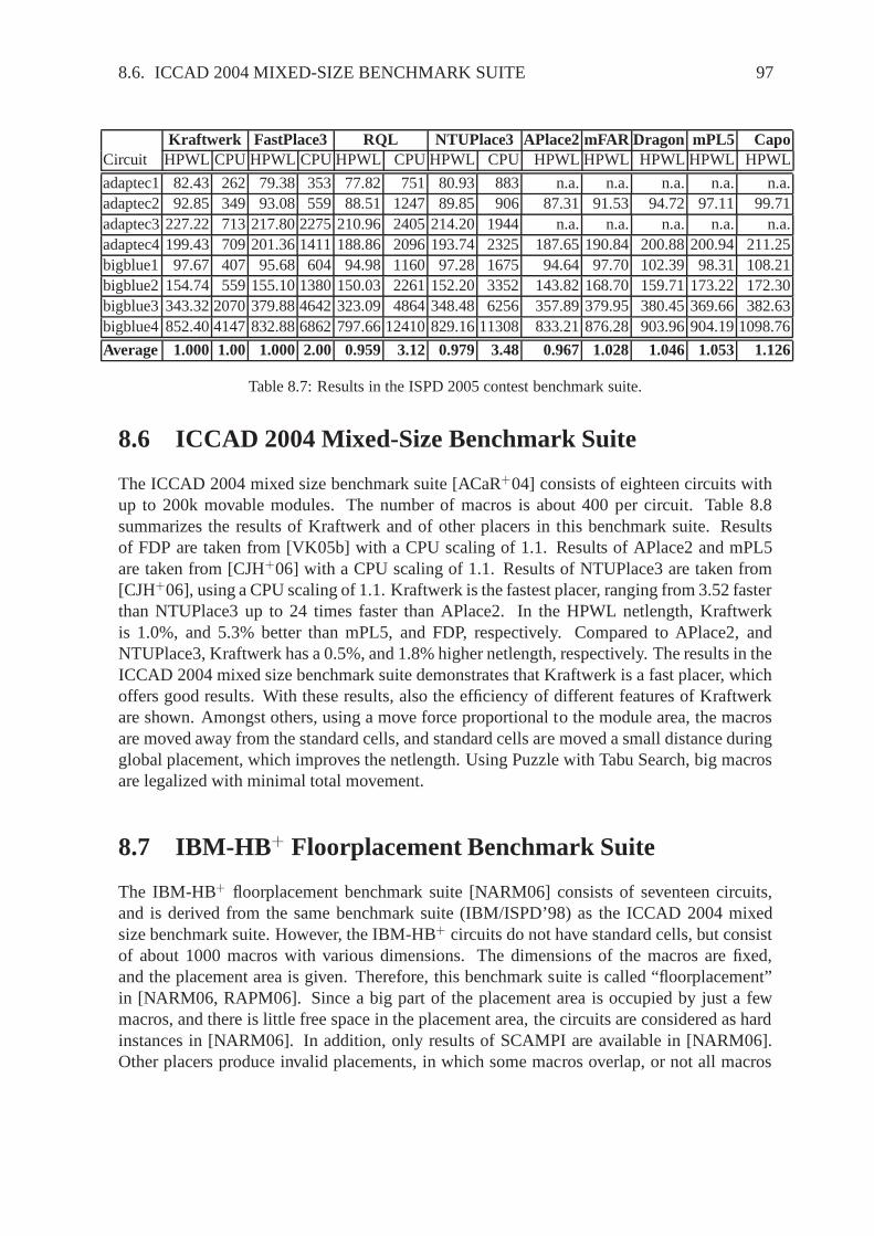
2.1 Global Placement
Global placement means to spread the modules roughly on the chip, resulting in a placementwith few overlaps. In the previous decades, different algorithms for global placement weredeveloped. They differ mainly in the way how the wirelength is minimized, and how themodules are spread on the chip. Figure 2.1 categorizes different techniques, and lists thenames of different state-of-the-art placers. Some of thesetechniques are able to spread themodules without any overlap on the chip. However, they are mostly stopped if there is onlylittle overlap remaining. This overlap is removed in final placement then.
2.1.1 Greedy Placement
Placers based on greedy methods have in common to modify a given start placement over asequence of iterations, and accept only better placements according to their cost. Here, the
7
8 CHAPTER 2. STATE OF THE ART
Timberwolf
AlgorithmSimulatedAnnealing
GeneticCapoDragonFengShui
Min-Cut
Partitioning
BonnPlacehATP
GordianPROUD
Quadratic
Force-Directed
RQLFDP
FARmFARFastplaceKraftwerk
mPLAPlace
NTUPlaceVaastu
Nonlinear
Global Placement Technique
StochasticGreedy ClusterGrowth
Analytical
Linear
Eigenvalues
Warping
WARP
Figure 2.1: Different placement techniques and names of various placers.
start placement can be random, and the cost is mainly a combination of wirelength and over-lap. Due to the fact that only better placements are accepted, greedy placers are likely toget stuck in a local minimum, i.e., they will probably not findthe optimal solution. In prin-ciple, greedy placers modify the placement by permuting modules, either just two modules[HK72, Shu75, Sch76, Bla85a, Bla85b, CP80, IKB83, KP77, HWA76], or three and moremodules [HWA76, Got79, Got81]. However, only for circuits with just a few modules, allpossible modifications can be tested. For bigger circuits, only neighboring modules can bepermuted in practicable runtime. Therefore, heuristics were developed to decide which mod-ules are best to permute [Qui75, HWA76, Got79, Got81]. The main drawback of greedyplacers is that they only do a local optimization of the placement. Thus, they highly dependon the start placement.
2.1.2 Cluster-Growth
Placers based on cluster-growth iteratively cluster new modules around already placed mod-ules. Here, the first placed modules can be random. The strategy of cluster-growth placerscan be viewed as bottom-up: starting from some placed modules, more and more modulesare placed, until all modules are placed. The decision, which modules are clustered, is donebased on a cost function representing the wirelength and themodule overlap. Placers usingthis method are for example [SU72, HK72, Shu75, Sch76, HWA76, KP77, Got79, Got81,DK87, LM90, Mul90, YK92, KK92, Lee93, SSL93]. These approaches have good results forsmall circuits, but degrade with increasing numbers of modules per circuit. This problem isdue to the local view of the method, and due to the high dependence on the start placement.
2.1.3 Min-Cut Placement
In contrast to the bottom-up strategy of cluster-growth placers, placers based on min-cutare following a top-down technique. Here, the placement area and the circuit are recur-
2.1. GLOBAL PLACEMENT 9
sively partitioned. In doing so, parts of the circuit are assigned to parts of the placementarea. The recursive process is done until each module is assigned to a unique part of theplacement area, which results in a placement with no or just little overlap. The partition-ing of the circuit is driven by minimizing the wirelength. Inprinciple, this is achievedby minimizing the number of nets cut (⇒ min-cut) by a partition. However, partitioninga circuit is a NP-hard problem [SH86]. Therefore, differentheuristics were developed forthis task [KL70, SK72, FM82, GB83, Kri84, Saa93, LLLC96, DD96b, DD96a, KAKS97,AHK97, CLL+97, ACH+97]. Beside the improvement in partitioning the circuit, the par-titioning of the placement area was also improved. The first min-cut placers divided theplacement area in two parts (bi-partitioning) in each step of the recursive placement process.[Bre77a, Bre77b, Cor79, Lau79, SH80, BH83, DK83, DK85, LD86, Zim88, SC88]. Lateron, four parts [SK87, SK88, Apt90, HK97], and even eight parts [San89, Vij89, ML90] wereused. Modern min-cut placers are for example Capo [RPA+05], Dragon [TYC05], and Feng-Shui [AOL+05].
2.1.4 Stochastic Placement
Stochastic placers combine the wirelength and the module overlap in one cost function, andminimize this cost function with stochastic methods. Stochastic methods means to createrandomly sets of placements in a sequence of iterations. In the end, the placement with thelowest cost function is chosen as the result. Stochastic placers can easily extend the costfunction in order to consider different objectives or various constraints. Moreover, stochasticplacers are able to escape from local minima, and are even able to find the optimal solution forthe placement problem. However, stochastic optimization in general needs a lot of samples(placements), and thus, stochastic placers are only practicable for circuits with a low numberof modules. In principle, there are two main methods of stochastic optimization: simulatedannealing and evolutionary algorithms.
Simulated Annealing
Simulated Annealing [KGV83] follows the annealing processin metallurgy: a hot metal iscooled (over time) such that in the end, it is most perfect (one crystal, no defects). As anoptimization method, Simulated Annealing starts with an arbitrary start configuration (place-ment). Over the iterations, new configurations are created randomly by so called “moves”. Amove for a placement can be to choose randomly a module, and tochange randomly its loca-tion. Each new configuration is given a cost, and a decision ismade if the new configurationis accepted, and thus replaces the best-so-far configuration. This decision is done based on thecost of both configurations, and based on the current temperature. The temperature is high atthe start, and is decreasing over the iterations. As a result, worse configurations are acceptedat the start of the optimization process, in order to escape from local minima. At the end, onlybetter configurations are accepted. The method of decreasing the temperature affects highlythe quality of the solution [Whi84, HRSV86, LD88, BKT93].
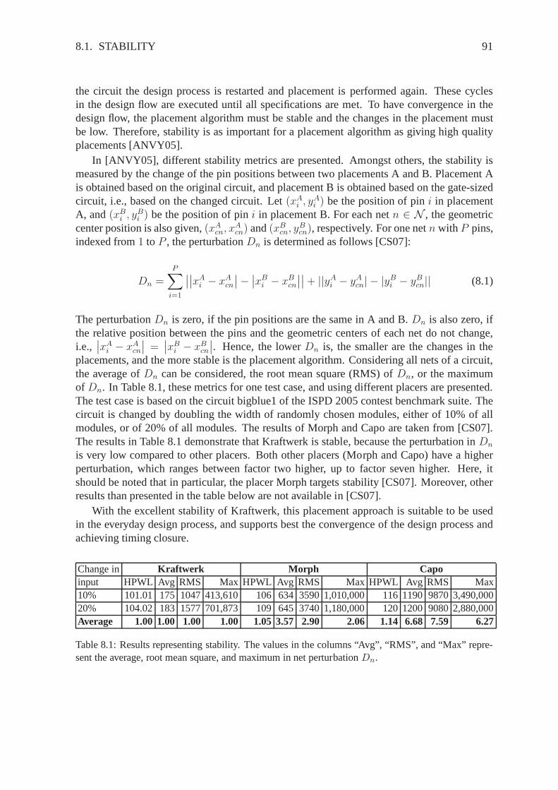
The authors of [RSV85, vLA87, Sec88, OvG89, AK89] showed that simulated anneal-ing is able to find the global optimum. Moreover, the basic operations of the optimization
10 CHAPTER 2. STATE OF THE ART
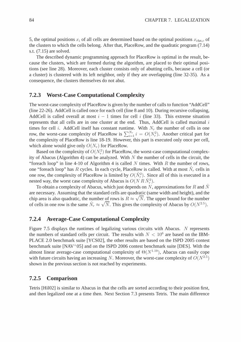
techniques are easy to implement. Hence, this technique wasvery popular for placement inthe past [SSV85, NSS85, SSV86, WL86, Sec88, WLL88, MFNK96, NFMK96]. However,the number of configurations necessary to find the optimum increases dramatically with thecomplexity, i.e., the number of modules per circuit. Therefore, different heuristics were usedalong with simulated annealing to cope with the increasing number of modules per circuit[MG88, HCC92, SKK+93, SS95, SW97]. A typical representative of a stochastic placer isTimberwolf [SS93]. Today, simulated annealing is rarely used to place circuits with millionsof modules.
Evolutionary Algorithms
Evolutionary algorithms use mechanisms inspired by biological evolution: heredity, mutation,selection, and survival of the fittest. In placement, evolutionary algorithms start by creating aset of random placements. In an iterative process, new placements are created based on currentplacements (heredity), and based on random changes (mutation). Then, the new placementare selected according to their cost. Over the iterations, the better placements survive, andat the end, a good placement is found. In principle, the basicoperations of evolutionaryalgorithms are simple, and the optimization can be run in parallel using numbers of computers.However, the runtime is still high for modern circuits. Evolutionary algorithms for placementare presented in [CP86, CP87, KB89, SM90, KB91, RR96, EK97].
2.1.5 Analytical Placement
Analytical placers are based on an analytical cost function, which is continuous and in mostcases differentiable. The minimum of the analytical cost function is determined by numericaloptimization. Mostly, the cost function represents the wirelength, and sometimes it is a com-bination of wirelength and overlap. Depending on the cost function, analytical placers can besubdivided in linear, quadratic and non-linear placers.
Linear Placement
Linear placers are using a linear cost function, and remove the module overlap by linearconstraints between the modules. This gives a linear program. However, such programs havea high computational complexity. Hence, linear placers like [WM87, HWM86, WM88, JK89,RC06] can only be used for circuits with a low number of modules. The analytical costfunction in linear placement can be non differential (e.g.,using the absolute value function).In all other analytical placement approaches, the cost function is differentiable.
Quadratic Placement
All quadratic placers represent the wirelength in a quadratic cost functionΓ:
Γ =1
2
∑
i,j
wx,ij(xi − xj)2 + wy,ij(yi − yj)
2 (2.1)
2.1. GLOBAL PLACEMENT 11
pi = (xi, yi) is the position of modulei. Γ is the sum of the weighted quadratic Euclideandistances between pairs of modules (i andj). The pairwise connections are called two-pinconnections. To represent the wirelength by two-pin connections inΓ, a net model is neces-sary in quadratic placement. Next Section 2.3 gives an overview on net models in general, andon state-of-the-art net models for quadratic placement. Amongst others, this thesis presents anovel net model for quadratic placement.
Representing the positions of allN movable modules in vectorp =(x1, x2, ..., xN , y1, y2, ...yN)T , the sum notation of the quadratic cost function (2.1) can berepresented in a matrix-vector notation:
Γ =1
2pT Cp + pTd + const (2.2)
Matrix C represents the connections between movable modules, and vector d reflects theconnections between movable and fixed modules. Fixed modules are for example I/O pins(input/output pins). By minimizingΓ, quadratic placers obtain the module positionsp withminimal netlength, which is the optimal placement. Since minimizing just the netlength re-sults in a lot of module overlap, quadratic placers need a method to reduce the overlap. De-pending on this method, quadratic placers can be subdividedinto three categories: based oneigenvalues, based on partitioning, and based on forces.
Eigenvalue-Based Quadratic Placement
Quadratic placers based on Eigenvalues assume that all modules are movable, i.e.,d = 0 in(2.2). To reduce the module overlap, and to spread the modules on the placement area, theseplacers are using the constraintpTp = const. Combining this constraint with the quadraticcost functionΓ by Lagrangian relaxation gives a new function, whose minimum is found bysetting its derivative (with respect toxi andyi) to zero. This results inCp − λp = 0, whichis similar to determining the Eigenvalues and Eigenvectorsof C. Then, the module positionsare given by the Eigenvectors with the lowest Eigenvalues. Eigenvalue quadratic placers arefor example [Hal70, Ott82a, Ott82b, FYSK83, Bla85a, Bla85b, FK86]. Since computingEigenvalues and Eigenvectors is complex, quadratic placers based on this technique are rarelyused to place state-of-the-art circuits with millions of modules.
Partitioning-Based Quadratic Placement
In order to reduce the module overlap, partitioning-based quadratic placers divide recursivelythe circuit and the placement area, and assign parts of the circuit to parts of the placement area.In contrast to min-cut placers, which use a similar technique for placement, partitioning-basedquadratic placers minimize a quadratic cost function in each step of the recursive placementprocess. In quadratic placement based on partitioning, different techniques are used to par-tition the placement area, to partition the circuit, and to hold the modules in the placementregion to which they are assigned.
The authors of [WWM82, Wip85] presented a placer, which firstplaces the modules byminimizing the quadratic cost function, and then assigns modules to placement regions us-
12 CHAPTER 2. STATE OF THE ART
ing a technique similar to min-cut. In [CK83, CK84], a methodis described, which recur-sively partitions the placement area in two regions. In eachiteration of recursion, the posi-tions of the modules are used to partition the circuit, and toassign the modules to placementregions. To place the modules in one region, the modules of the other regions are fixed,and linear constraints (center-of-mass constraints) are used to spread the modules. PROUD[TKH88a, TKH88c, TKH88b] is similar to this technique, but does not utilize linear con-straints. To spread the modules in one region, the fixed modules of the other regions areprojected to the border of the current region. With the recursion, the placement regions, andthe number of modules assigned to them are continuously decreasing. By placing only themodules in one region, and fixing all other modules, the placement problem is solved moreand more locally. This will decrease the quality of the solution. In contrast to this, Gor-dian [KSJ88, KSJ89, Kle89, KSJA91] places all modules concurrently in all iterations ofthe recursive partitioning process. The partitioning is driven by the module positions. Tohold the modules, which are assigned to one placement region, in this region, Gordian usescenter-of-mass constraints. GordianL [SDJ91, Sig92] improves the method for partitioningthe placement area, and introduces weights in the quadraticcost function, which are used forlinearization the quadratic wirelength.
BonnPlace [Vyg97, BS05], and hATP [NRA+06] partition the placement area in four re-gions in each step of recursive placement process. A min-cost-max-flow is used to partitionthe circuit, and to assign modules to placement regions. To hold the modules in their place-ment regions, BonnPlace and hATP use center-of-mass constraints, and so called “terminals”.These terminals arise while cutting the nets by partitioning. In other words, the terminals con-nect two nets of two partitions, which where formerly one netin one partition. The terminalsare located at the border between two partitions, are treated as fixed modules, and results inthat the modules in each placement partition stay within itspartition. In addition, with thefixed terminals, each placement partition can be placed concurrently using different CPUs.This improves runtime, but advanced methods for positioning the terminals are necessary inorder to prevent a decline in the placement quality.
In general, partitioning quadratic placers are able to place modern circuits in reasonableruntime. Since they reduce the module overlap by partitioning, and mostly ignore the moduledimension here, they are problematic if the modules are of different dimension like in mixed-size circuits.
Force-Directed Quadratic Placement
The two-pin connections used in (2.1) for the quadratic costfunction Γ can be viewed aselastic springs. This creates a spring system, andΓ represents the total energy of the springsystem. The derivative ofΓ is the “net” force, created by the springs:Fnet = Cp+d. Settingthis force to zero gives the module positions with minimal wirelength, which equals the equi-librium state of the spring system. In other words, the springs, i.e., the two-pin connections,of quadratic placement create a force, which attracts the modules. Force-directed quadraticplacers utilize an additional forceFadd to spread the modules on the placement area. Thisspreading is done in a sequence of placement iterations. Each iteration starts with a givenplacement. Then, an additional force is determined. Setting the sum of the net force and the
2.1. GLOBAL PLACEMENT 13
additional force to zero results in a system of linear equations. This system can be solvedefficiently with respect top. At the end of each placement iteration, the modules are placedto the positions described byp.
Different approaches exist for the additional forces. In [FCW67], the additional force ismodeled in that all modules are repelling each other. However, this results in a high number ofadditional forces. To reduce the computational complexity, other approaches utilize repellingforces only between unconnected modules. In [Sca71, Qui75,QB79, AJK82, JJA83, Kir84,For87, Jus87], the repelling force is constant over the distance between the not connectedmodules. In [FCW67, QB79, Kir82, Waw88], the repelling force is reciprocal to the distance.Another modification is to model the overlaps between the modules rather than the modulesthemselves as the source for the repelling force. In [Sca71,Shu75, Rob83, SD85, SB87,AA88, KKM91] overlaps between modules are repelling each other. The overlap betweenmodules and the border of the placement region is modeled in [FCW67, Shu75, KKM91] asthe source for the repelling force. In [Joh87], the triangulation of the placement area based onthe module positions is used to determine a force, which spreads the modules on the placementarea.
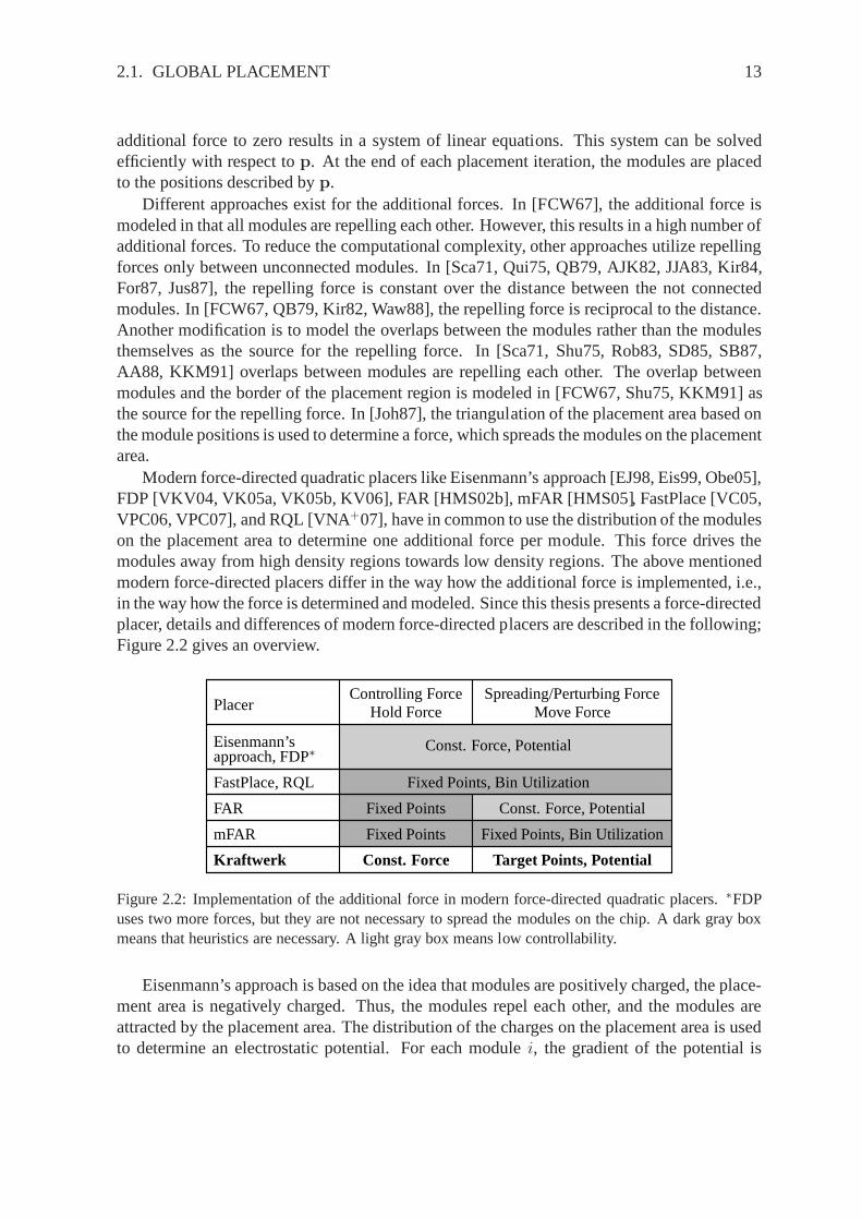
Modern force-directed quadratic placers like Eisenmann’sapproach [EJ98, Eis99, Obe05],FDP [VKV04, VK05a, VK05b, KV06], FAR [HMS02b], mFAR [HMS05], FastPlace [VC05,VPC06, VPC07], and RQL [VNA+07], have in common to use the distribution of the moduleson the placement area to determine one additional force per module. This force drives themodules away from high density regions towards low density regions. The above mentionedmodern force-directed placers differ in the way how the additional force is implemented, i.e.,in the way how the force is determined and modeled. Since thisthesis presents a force-directedplacer, details and differences of modern force-directed placers are described in the following;Figure 2.2 gives an overview.
Spreading/Perturbing ForceMove Force
approach, FDP∗
FastPlace, RQL
FAR
mFAR
Kraftwerk
Controlling ForceHold Force
Fixed Points
Const. Force
Fixed Points
Const. Force, Potential
Fixed Points, Bin Utilization
Placer
Fixed Points, Bin Utilization
Target Points, Potential
Const. Force, Potential
Eisenmann’s
Figure 2.2: Implementation of the additional force in modern force-directed quadratic placers.∗FDPuses two more forces, but they are not necessary to spread themodules on the chip. A dark gray boxmeans that heuristics are necessary. A light gray box means low controllability.
Eisenmann’s approach is based on the idea that modules are positively charged, the place-ment area is negatively charged. Thus, the modules repel each other, and the modules areattracted by the placement area. The distribution of the charges on the placement area is usedto determine an electrostatic potential. For each modulei, the gradient of the potential is
14 CHAPTER 2. STATE OF THE ART
determined, and the gradients are accumulated in the additional force over the placement it-erations. The additional force in Eisenmann’s approach is modeled as constant force, i.e., theforce does not depend onp.
Using a constant force is one way to model a force. Another wayto model a force is touse fixed points (each located atpi), and connect each module to its fixed point by an elasticspring having the strengthsi. This spring creates the force then.
Fspring
i = si (pi − pi) (2.3)
The authors of [HMS02b] showed that using fixed points are a generalization of using aconstant force, and they showed that fixed points control theplacement better than constantforces do. In principle, the controllability is improved because each module is moved at mostto its fixed point in each placement iteration. Using a constant force, the movement is notlimited.
FDP is similar to Eisenmann’s approach in that the gradientsof the potential are accumu-lated in a constant force to spread the modules on the chip. Inaddition, FDP used two forcesto stabilize the placement algorithm, and to improve the netlength. These two forces are mod-eled by fixed points in FDP. Similar to Eisenmann’s approach,FAR utilizes an electrostaticpotential to determine a force, which spreads the modules onthe chip. This additional force ismodeled as a constant force. Instead of accumulating the spreading force over the iterations,FAR uses a second additional force for each module to controlthe placement process. Thisforce is modeled by fixed points and is determined by achieving force equilibrium at the startof each placement iteration. The main difference between FAR and mFAR is that mFAR usesa local bin utilization to determine the spreading force, and the spreading force is modeled byfixed points. Using a local bin utilization, the spreading force has a local view, as the forceof one module depends only on the surrounding modules. In contrast to this, the (spreading)force in Eisenmanns’ approach, FAR, and FDP has a global view, i.e., the force of one moduledepends on all modules. This is because the force is based on potential formulation there, andthe potential represents all modules.
Instead of accumulating one additional force over the placement iterations, or using twoadditional forces, FastPlace and RQL are using a different method to spread the modules. Ineach placement iteration, a local bin utilization is determined similar to mFAR. The addi-tional force for one modulei is then determined as follows. Modulei is temporary placed tothe position determined by the local bin utilization. This can be viewed as a local diffusionprocess. Then, the force is determined, which holds modulei at its temporary position. Afterthat, modulei is put back to its original position. After determining the additional force forall modules, the new positions for all modules are obtained by setting the sum of the net forceand the additional force to zero. The additional force is modeled by fixed points. In FastPlace,the fixed points are located at the border of the placement regions. RQL uses a location be-tween the border and the module position. In addition, RQL modulates the additional force,which means that for some modules, the additional force is ignored. With this, the modulesare reordered during placement, which can improve the netlength. On the other hand, theconvergence of the placement algorithm can be harmed.
In summary, fixed points are widely used in modern force-directed quadratic placers. Thelocations of the fixed points are all determined in that a force is given. This force is to be
2.1. GLOBAL PLACEMENT 15
represented by the spring connection between each module and its fixed point. In this case,where the force is given, a good heuristic is necessary to obtain suitable locations of thefixed points. This is a well-known critical problem of using fixed points [HMS02b, HMS05,VNA+07].
Fspring
i
∣∣∣pi=p′
i
= ei ⇔ pi = p′i −
1
si
ei (2.4)
In (2.4), the forceei of modulei is given, and the module is located atp′i, i.e.,pi = p′
i.If the strengthsi of the spring is too low, the fixed pointpi is too far away from the modulepositionp′
i, and the force is modeled like a constant force, resulting inlow controllability. Ifthe strengthsi is too high, the fixed point is too near to the module, and the module movementis highly limited. Thus, all modern force-directed placers, using fixed points, rely on heuristicsfor good values ofsi. The force-directed quadratic placer Kraftwerk, as presented in thisthesis, also uses fixed points (called “target points”), butdoes not depend on critical heuristics.Rather, the locations of the target points are directly given by the gradients of an electrostaticpotential. In other words, not the force is given, but the location of the target points. InKraftwerk, two forces are used: a moving force, modeled by target points, and a hold force,modeled as a constant force. The constant hold force does notreduce controllability of theplacement process, but enforces the convergence.
Nonlinear Placement
Nonlinear placers are based on a nonlinear cost function, which is even not quadratic. Plac-ers based on nonlinear cost functions have appeared in the recent years, after developing anefficient representation of the wirelength by a log-sum-expfunction [NDS01]. The majordrawback of nonlinear placers is that nonlinear numerical optimization takes high runtimes.Nonlinear placers differ mainly in the way how the module overlap is removed.
Density-Driven Nonlinear PlacementDensity-driven nonlinear placers are using the distribution of the modules on the placementarea (i.e., the module density at various points) to determine a nonlinear function, whichrepresents the module overlap, and which is continuous and differentiable. This function iscombined with the wirelength function in a total cost function, and the total cost functionis minimized by nonlinear numerical optimization. In this way, the modules are iterativelyspread over the placement area. Examples for density-driven nonlinear placers are APlace[KW05a, KRW05], mPL [CCS05], and NTUPlace [CJH+06].
Nonlinear Placement Based on Pseudo NetsNonlinear placers based on pseudo nets are using additional“pseudo” nets (one for each mod-ule). This is similar to the fixed point approach used in force-directed quadratic placement.Minimizing the wirelength of the nets and the pseudo nets, the modules are spread iterativelyover the placement area. In each placement iteration, Vaastu [AM07] is using a min-cost-max-flow to assign modules to placement regions. Then, the pseudo nets are created betweeneach module and the center position of the placement region to which the module is assigned.In other words, and considering force-directed quadratic placement, the fixed points of the
16 CHAPTER 2. STATE OF THE ART
pseudo nets are determined by a min-cost-max-flow approach in Vaastu. Other nonlinearplacers using pseudo nets are not known up to now.
2.1.6 Warping Placement
Placers based on warping start with an initial placement, and are using approaches of com-putational geometry to deform the placement area, and thus moving the modules indirectly.The deformation of the placement area is driven by minimizing the wirelength and the mod-ule overlap. Placers based on warping are for example [XMFR04, XR07, CS07]. To obtainthe initial placement, warping placers usually follow quadratic placement and minimize thequadratic wirelength.
2.2 Multilevel Approach
To place “large” circuits, i.e., circuits with a high numberof modules, some placement ap-proaches are following a hierarchical approach. Min-cut placers, placers based on cluster-growth, and some partitioning placers are per se hierarchical, because not all modules of thecircuit are placed simultaneously in all placement iterations.
A general hierarchical approach to cope with “large” circuits is the multilevel approach,which can be used for all placement techniques. Starting from the “flat” circuit, which consistsof all modules, the modules are clustered over a few levels during the coarsening phase. Then,the coarsest circuit is placed. In the refinement phase, the placement of the previous levelis used as input, the clusters are declustered, and the new “refined” circuit is placed. Therefinement is done until the flat circuit is placed. Since onlysome placement iterations arespent in each level of refinement, and in particular only someiterations for the flat circuit,the runtime decreases with the multilevel approach. However, the major drawback of themultilevel approach, and of all hierarchical approaches ingeneral, is that a good heuristic isnecessary to partition or cluster the circuit. This is because optimal partitioning is an NP-hard problem [SH86]. In addition, using a hierarchical approach, the placement problem issolved more locally then using a flat approach, where all modules are placed concurrently inall placement iterations.
2.3 Net Models
The previous sections described different techniques to solve the placement problem. Thegeneral objective of the placement problem is to minimize the total length of all nets. Thisobjective is used because a placement with minimal netlength is usually optimal also in otherobjectives like area consumption, routability, timing (length of the critical path), etc. Thissection describes how to measure the length of one net. There, the net is represented bygraphs, different net metrics are shown, and net models necessary for quadratic placement arepresented.
2.3. NET MODELS 17
2.3.1 Graphs and Metrics
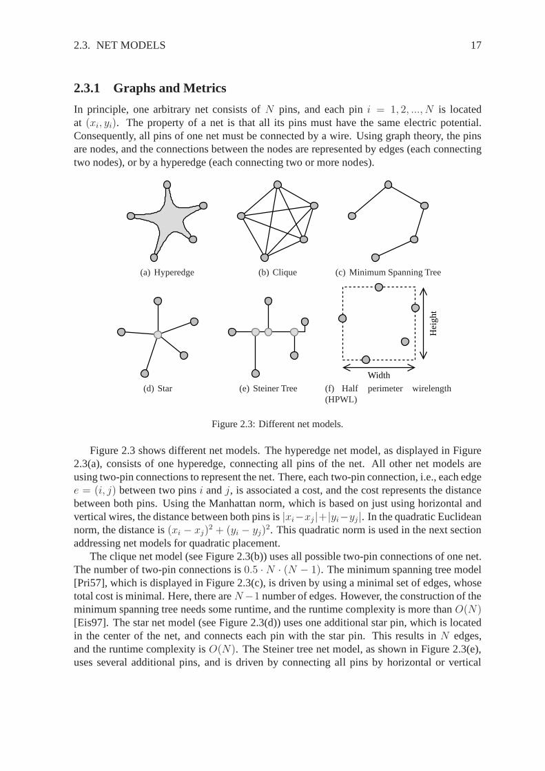
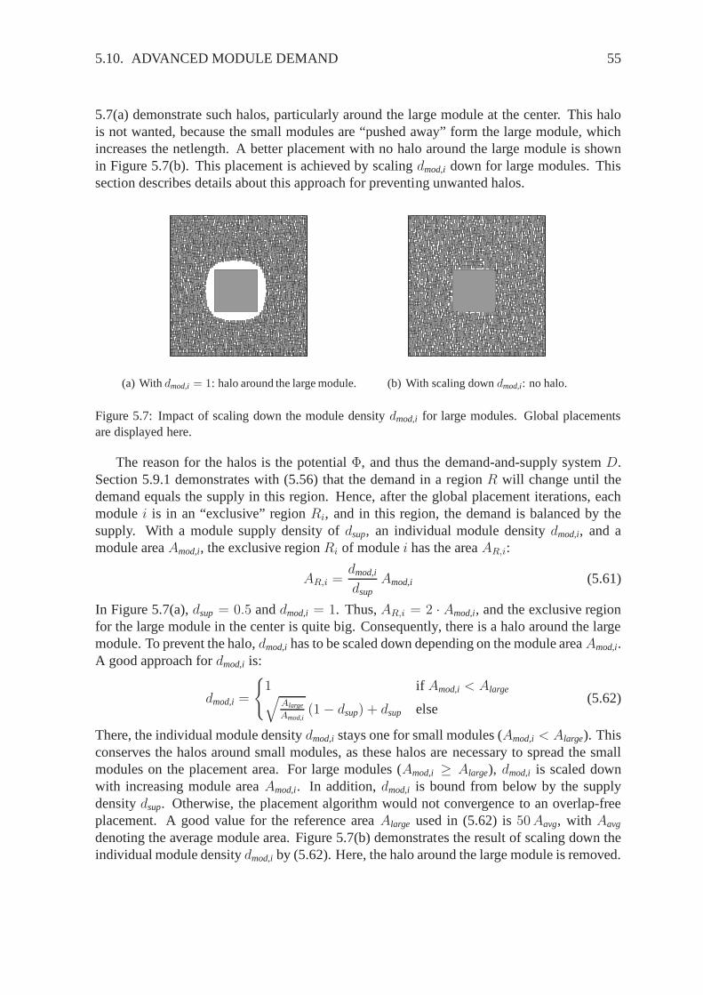
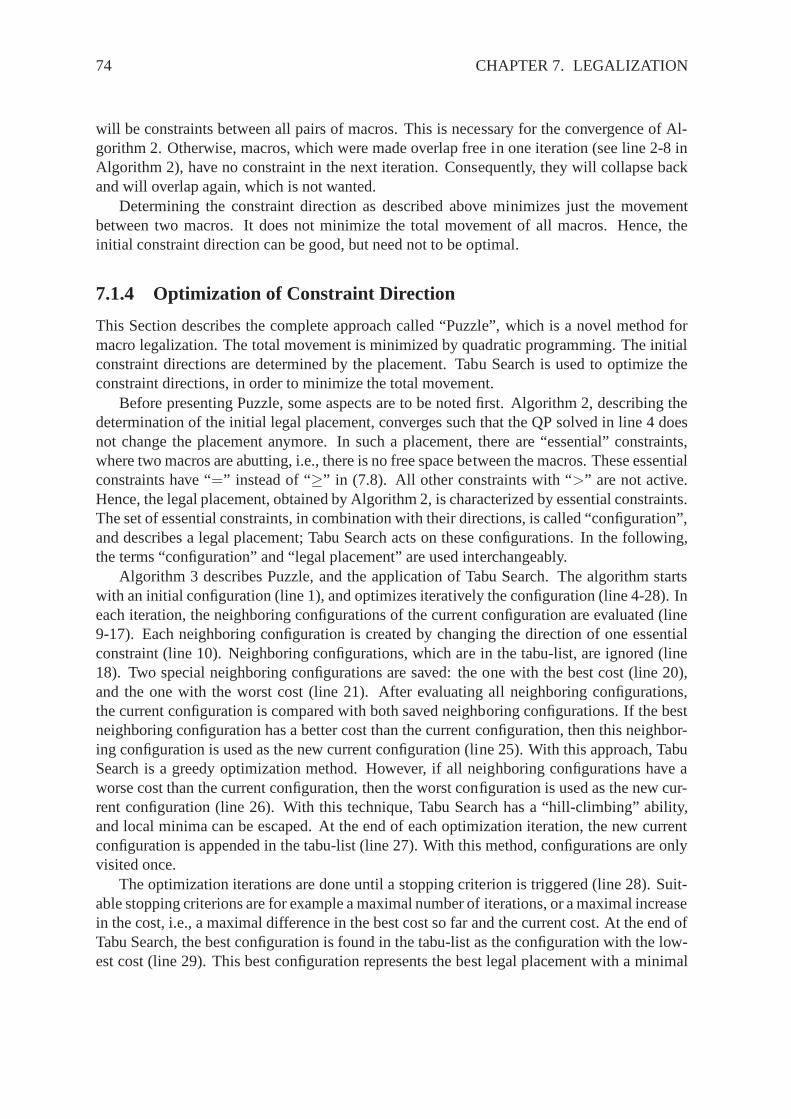
In principle, one arbitrary net consists ofN pins, and each pini = 1, 2, ..., N is locatedat (xi, yi). The property of a net is that all its pins must have the same electric potential.Consequently, all pins of one net must be connected by a wire.Using graph theory, the pinsare nodes, and the connections between the nodes are represented by edges (each connectingtwo nodes), or by a hyperedge (each connecting two or more nodes).
(a) Hyperedge (b) Clique (c) Minimum Spanning Tree
(d) Star (e) Steiner Tree
Width
Hei
gh
t
(f) Half perimeter wirelength(HPWL)
Figure 2.3: Different net models.
Figure 2.3 shows different net models. The hyperedge net model, as displayed in Figure2.3(a), consists of one hyperedge, connecting all pins of the net. All other net models areusing two-pin connections to represent the net. There, eachtwo-pin connection, i.e., each edgee = (i, j) between two pinsi andj, is associated a cost, and the cost represents the distancebetween both pins. Using the Manhattan norm, which is based on just using horizontal andvertical wires, the distance between both pins is|xi−xj |+|yi−yj |. In the quadratic Euclideannorm, the distance is(xi − xj)
2 + (yi − yj)2. This quadratic norm is used in the next section
addressing net models for quadratic placement.The clique net model (see Figure 2.3(b)) uses all possible two-pin connections of one net.
The number of two-pin connections is0.5 ·N · (N − 1). The minimum spanning tree model[Pri57], which is displayed in Figure 2.3(c), is driven by using a minimal set of edges, whosetotal cost is minimal. Here, there areN−1 number of edges. However, the construction of theminimum spanning tree needs some runtime, and the runtime complexity is more thanO(N)[Eis97]. The star net model (see Figure 2.3(d)) uses one additional star pin, which is locatedin the center of the net, and connects each pin with the star pin. This results inN edges,and the runtime complexity isO(N). The Steiner tree net model, as shown in Figure 2.3(e),uses several additional pins, and is driven by connecting all pins by horizontal or vertical
18 CHAPTER 2. STATE OF THE ART
edges only. In the minimal Steiner tree, the edges are chosensuch that the total cost of alledges is minimal. Finding such an optimal Steiner tree is known to be a NP-hard problem[GJ77]. However, there exist numbers of algorithms, which find a near-optimal Steiner treein practicable runtime [Han66, Hwa79, Ser81, CRS88, HVW90,GRSZ94, Chu04]. Sincerouting of a net is similar to constructing the minimal Steiner tree, the routed wirelength,i.e., the wirelength after routing, is best approximated bylength of the minimal Steiner tree.However, routing is more complex than just constructing theminimal Steiner tree, as morethings have to taken into account in routing. For example, there is only a limited numberof routing tracks available in a chip, which limits the resources for routing. Or not only thewirelength is to be minimized in routing, but also the numberof vias.
The half-perimeter wirelength (HPWL), as illustrated in Figure 2.3(f), is rather a metricfor the netlength, than a net model. Here, “half-perimeter”means the half-perimeter of thesmallest rectangle enclosing all pins of the net. The width of this rectangle is given byw =max xi − min xi, and the height is given byh = max yi − min yi. Then, the HPWL isw + h. The HPWL equals the length of the minimal Steiner tree for nets with two or threepins [Han66]. For nets with four and more pins, the HPWL is a lower bound. Since mostof the nets of a circuit are two and three pin nets, the HPWL is an efficient estimation ofthe length of the minimal Steiner tree [Chu04], and consequently, it is an efficient estimationof the routed wirelength [Ser81, SKAS88]. Here, efficient means that the HPWL offers lowruntime and good approximation.
2.3.2 Net Models for Quadratic Placement
Quadratic placement is based on two-pin connections, and minimizing a quadratic cost func-tion (2.1), which represents the sum of the quadratic lengths of the two-pin connections.Since the runtime complexity of determining suitable two-pin connections is practicable inthe clique and the star net model, these net models are used widely in quadratic placement.Traditionally, the weights of the two-pin connections are used to linearize the quadratic length,and to approximate the quadratic cost function to the HPWL metric.
Considering one net withN pins, a weight of1/N in the clique net model adapts itsquadratic costs to the cost of the corresponding star net model [Sig92, VC05]. Hence, cliqueand star net model can be used interchangeably. The authors of [Vyg97, BS05] use an addi-tional weight of1/N − 1 for each net, in order to prevent that nets with a high number of pinsare dominating the quadratic cost function. In [SDJ91, Sig92], the additional weight for eachnet is2/N , and a linearization weight for each two-pin connection is used, in order to adaptthe quadratic cost to the HPWL.
Since the clique and the star net models have different characteristics, and both can beused concurrently, there is a trade-off between both net models [EJ98, Eis99, VC05]. Theclique net model has no additional star pin, but a complexityof O(N2) in the number of two-pin connections. The star net model introduces one additional star pin per net, but has onlyO(N) two-pin connections. To minimize the quadratic cost function in short runtime, thenumber of two-pin connections, and the number of pins shouldbe as low as possible. In anaverage circuit, most of the nets have two or three pins, and nets with a high number of pinsare rare. Hence, the clique model is used for small nets, i.e., for nets with a about six or less
2.4. ROUTABILITY-DRIVEN PLACEMENT 19
pins, as the number of two-pin connections is reasonable here. For big nets, the star net modelis used, as the number of two-pin connection is low here, and the number of additional starpins is reasonable. Using clique and star net models concurrently in a circuit gives the hybridclique/star net model.
The authors of [BS05] propose a net model suitable for partitioning quadratic placers,which is based on the star net model, but introduces additional pins (so called “terminals”) forthose nets, which cross the border of two placement partitions. In [OJ04a, Obe05], a methodis described, which integrates the minimal Steiner tree in the quadratic cost function. This isused to obtain better timing-driven placements. However, determining a minimal Steiner treeis time consuming.
This thesis presents a new net model, which accurately represents the HPWL in thequadratic cost function. Compared to a hybrid clique/star net model, the new net model offersbetter placements in lower runtime.
2.4 Routability-Driven Placement
In the layout synthesis of an integrated circuit, the modules are placed first, and the nets arerouted then. These are two separate steps, mostly done by twodifferent computer programs.Placement traditionally targets to minimize the total wirelength, which in general improvesroutability. However, the placed circuit may not be routable, because there are so called“congested regions” on the chip, where too many wires are necessary to route the nets thanrouting tracks are available. In other words, the routing demand, created by the nets, exceedsthe routing supply, given by the routing layers. Due to such congested regions, the circuithas a high routed wirelength, or is even not routable. Therefore, besides minimizing the totalwirelength, placement has to be driven by routability, which means to remove the congestionsduring placement. To do routability-driven placement, twoproblems have to be solved. First,a fast and accurate method to estimate the congestions is necessary. This is because the exactinformations about congested regions would be given after routing, but routing itself takesenormous runtime. Second, the congestion estimation has tointegrated effectively in theplacer. This thesis presents novel solutions for both problems. Therefore, the state-of-the artin congestion estimation and in the integration in placement is described next.
2.4.1 Congestion Estimation
Assuming a constant routing supply, congestion estimationmeans to estimate the routingdemand. Most published methods to estimate the routing demand are using a grid structure todivide the chip area into a number of bins, and estimate the routing demand in each bin.
Based on the bounding box of one net, i.e., the smallest rectangle enclosing all pins of onenet, the authors of [lEC94] presented a simple method to estimate the routing demand in onebin: the routing demand of one net in one bin depends on the overlap between the boundingbox of the net and the bin. Another simple technique to estimate the routing demand in onebin is to use the pin density within this bin [BR02, ZD02]. A widely applied technique toestimate the routing demand is to use a routing model, which models possible routes of each
20 CHAPTER 2. STATE OF THE ART
net. The number of possible routes crossing the border of a bin reflects the routing demandin the bin. In most approaches based on routing models, multi-pin nets are broken down intotwo-pin connections by using a minimum spanning tree. Then,for each two-pin connection,different routes with different number of bends are modeled. The authors of [LKS02] useall possible routes for each two-pin connection. This probabilistic routing model is improvedin [KX03, SZJ06] by adjusting its result to the result obtained by routing. The authors of[WBG04] state that one- and two-bend routes are enough to model the routing demand. In[PC06], a fast global router is proposed, which uses different Steiner Trees to model thepossible routes of each net. In [YKS01, YKS02, HMS02a], the maximal routing demand of acircuit is estimated based on Rent’s Rule [LR71]. Another technique to estimate the routingdemand is the analysis of the distribution of the number of nets per bin [WYES00].
2.4.2 Integration in Placement
Estimating the routing demand in an efficient way is the first step to optimize routability dur-ing placement. The second step is to integrate the estimation of the routing demand in theplacement algorithm, in order to remove the congestions andto improve routability. Sincethe congested regions are characterized that the routing demand of the nets is higher than thesupply by the routing layers, there exist two main approaches to optimize routability. Thedirect approach reduces the routing demand in congested regions, and the indirect approachincreases the routing supply in congested regions. The routing supply can be increased, be-cause modules block some routing layers, and with a lower module density, more free spaceis available in the routing layers. The routing demand can bedecreased by replacing modules,such that the nets connected to the modules are moved out of the congested regions. The directapproach is often used as a post-process to tune an already placed circuit for routability. Apost-process utilizing Simulated Annealing is described in [lEC94, HMS02a, WS99]. A flow-based method is presented in [WYS00, WS00]. Linear programming is used in [LWH03].
The indirect approach to optimize routability is mostly used during placement. In [HYH+01,BR02], a quadratic placer is described, which inflates modules in congested regions. Theauthors of [PBS98] present a quadratic placer, which reduces module density in congestedregions by growing these regions. In [YCS03], a min-cut placer is shown, which allocateswhite space, i.e., reduces module density, in congested regions during top-down placement.
In the following, routability optimization in state-of-the-art placers is described. mPL[LXK +04, LXK+07] is a multilevel analytical placer based on non-linear optimization. mPLestimates the routing demand based on a two-pin connection routing model developed in[CCPY02]. Routability is optimized in global placement by moving certain modules out ofcongested regions in order to reduce the routing demand there. In final placement, a whitespace allocation (WSA) method is used, which is based on recursively partitioning the place-ment area, and shifting the cut lines according to the routing demand. Thus, mPL utilizesthe direct approach during global placement, and the indirect approach after wards in detailedplacement.
ROOSTER [RLM06], as a feature of Capo 10, is a min-cut placer.The placer modelsnets by Steiner trees [Chu04], and estimates the routing demand by a probabilistic routingmodel [WBG04]. The cut lines are shifted during global placement based on the routing de-
2.5. FINAL PLACEMENT 21
mand. During final placement, the WSA method of [LXK+04] is used. Therefore, ROOSTERapplies the indirect approach to optimize routability.
APlace [KW05b] is a multilevel analytical placer based on non-linear optimization. APlaceestimates the routing demand by a probabilistic routing model [KX03]. Routability is opti-mized during global placement by decreasing module densityin congested areas, i.e., by theindirect approach.
2.5 Final Placement
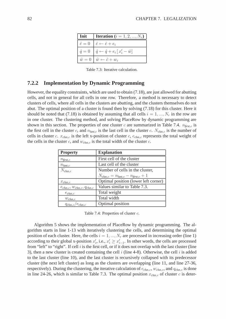
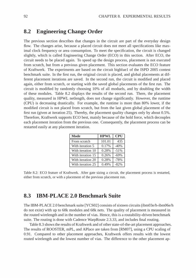
The global placement approaches proposed in Section 2.1 spread the modules roughly on thechip, while considering different objectives like total wirelength and routability. After globalplacement, final placement is done. Final placement itself consists mostly of two consecutivesteps: legalization and detailed placement. In legalization, the remaining overlap of the globalplacement is removed, and the modules are aligned to a row or grid structure if necessary.In detailed placement, the legal placement is improved suchthat the total wirelength is fur-ther reduced, or more complex objectives like design for manufacturing (DFM) [GKP05] ordesign for yield (DFY) [ABD+07] are considered. The common approach in detailed place-ment is to use small sliding windows in order to capture a low number of modules (about10 modules), and to do different transformations on this setof modules. For example, singlemodules are rotated, pairs of modules are exchanged, or all modules in the set are permuted[CKM00, CX06, LXK+07, PVC05, RPA+07]. In [KTZ99, BV00], a detailed placement ap-proach suitable for standard cell circuits is described. There, the modules in each row areplaced such that their total HPWL netlength is minimized. The ordering of the modules is notchanged here.
Since this thesis describes new approaches for legalization, this section focuses on thestate-of-the-art techniques for legalizing a global placement. To preserve the global placementas far as possible, the common objective of legalization is to move the modules as little aspossible. While most global placement approaches can deal with different circuit types likestandard cell circuits, macro cell circuits, and mixed sizecircuits, legalization approachesdiffer in the circuit type for which they are applicable. This difference in legalization isbecause of the different “design rules” for each circuit type. So, the modules of FPGA circuits,and the modules of sea-of-gates circuit have to aligned to a grid structure. The modules ofstandard cell circuits have to be aligned to rows. And the modules of macro cell circuits havenot to be aligned to rows. These design rules are mostly ignored during global placement asthe modules are spread just roughly on the placement area. Because of the difference in theapplication of the legalization approaches, the modules ofglobal placement are now calledstandard cells, or macros. In the following, state-of-the-art approaches for legalizing standardcell circuits are proposed. Most of the approaches are also applicable for FPGA circuits, andfor sea-of-gates circuits. In addition, modern methods forlegalizing macros are described. InChapter 7, novel approaches for legalizing these two circuit types are presented.
22 CHAPTER 2. STATE OF THE ART
12
3
47
5
6
(a) Global Placement
2
1
3
4
6
7
5
(b) Legal Placement
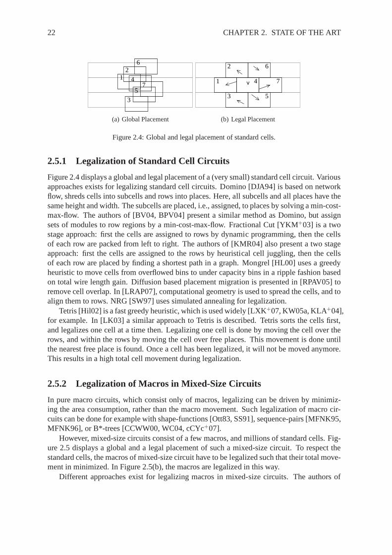
Figure 2.4: Global and legal placement of standard cells.
2.5.1 Legalization of Standard Cell Circuits
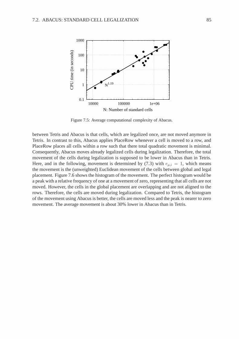
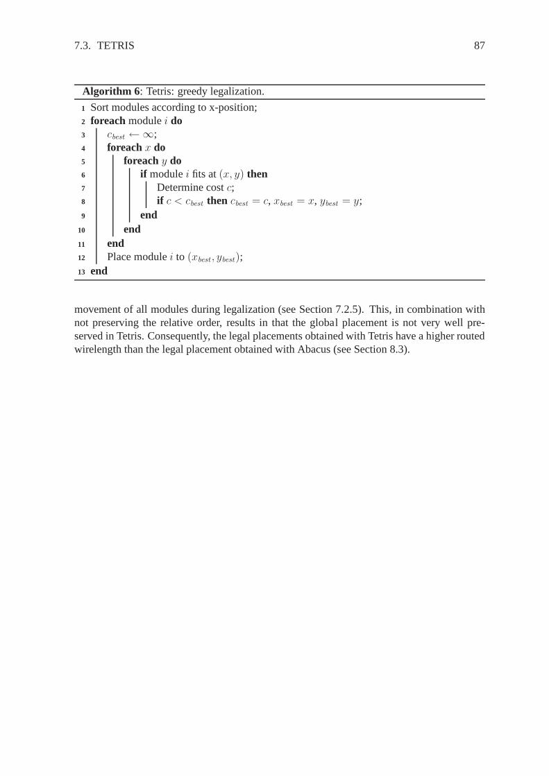
Figure 2.4 displays a global and legal placement of a (very small) standard cell circuit. Variousapproaches exists for legalizing standard cell circuits. Domino [DJA94] is based on networkflow, shreds cells into subcells and rows into places. Here, all subcells and all places have thesame height and width. The subcells are placed, i.e., assigned, to places by solving a min-cost-max-flow. The authors of [BV04, BPV04] present a similar method as Domino, but assignsets of modules to row regions by a min-cost-max-flow. Fractional Cut [YKM+03] is a twostage approach: first the cells are assigned to rows by dynamic programming, then the cellsof each row are packed from left to right. The authors of [KMR04] also present a two stageapproach: first the cells are assigned to the rows by heuristical cell juggling, then the cellsof each row are placed by finding a shortest path in a graph. Mongrel [HL00] uses a greedyheuristic to move cells from overflowed bins to under capacity bins in a ripple fashion basedon total wire length gain. Diffusion based placement migration is presented in [RPAV05] toremove cell overlap. In [LRAP07], computational geometry is used to spread the cells, and toalign them to rows. NRG [SW97] uses simulated annealing for legalization.
Tetris [Hil02] is a fast greedy heuristic, which is used widely [LXK +07, KW05a, KLA+04],for example. In [LK03] a similar approach to Tetris is described. Tetris sorts the cells first,and legalizes one cell at a time then. Legalizing one cell is done by moving the cell over therows, and within the rows by moving the cell over free places.This movement is done untilthe nearest free place is found. Once a cell has been legalized, it will not be moved anymore.This results in a high total cell movement during legalization.
2.5.2 Legalization of Macros in Mixed-Size Circuits
In pure macro circuits, which consist only of macros, legalizing can be driven by minimiz-ing the area consumption, rather than the macro movement. Such legalization of macro cir-cuits can be done for example with shape-functions [Ott83, SS91], sequence-pairs [MFNK95,MFNK96], or B*-trees [CCWW00, WC04, cCYc+07].
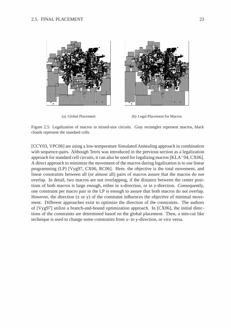
However, mixed-size circuits consist of a few macros, and millions of standard cells. Fig-ure 2.5 displays a global and a legal placement of such a mixed-size circuit. To respect thestandard cells, the macros of mixed-size circuit have to be legalized such that their total move-ment in minimized. In Figure 2.5(b), the macros are legalized in this way.
Different approaches exist for legalizing macros in mixed-size circuits. The authors of
2.5. FINAL PLACEMENT 23
(a) Global Placement (b) Legal Placement for Macros
Figure 2.5: Legalization of macros in mixed-size circuits.Gray rectangles represent macros, blackclouds represent the standard cells.
[CCY03, VPC06] are using a low-temperature Simulated Annealing approach in combinationwith sequence-pairs. Although Tetris was introduced in theprevious section as a legalizationapproach for standard cell circuits, it can also be used for legalizing macros [KLA+04, CX06].A direct approach to minimize the movement of the macros during legalization is to use linearprogramming (LP) [Vyg97, CX06, RC06]. Here, the objective is the total movement, andlinear constraints between all (or almost all) pairs of macros assure that the macros do notoverlap. In detail, two macros are not overlapping, if the distance between the center posi-tions of both macros is large enough, either in x-direction,or in y-direction. Consequently,one constraint per macro pair in the LP is enough to assure that both macros do not overlap.However, the direction (x or y) of the constraint influences the objective of minimal move-ment. Different approaches exist to optimize the directionof the constraints. The authorsof [Vyg97] utilize a branch-and-bound optimization approach. In [CX06], the initial direc-tions of the constraints are determined based on the global placement. Then, a min-cut liketechnique is used to change some constraints from x- to y-direction, or vice versa.
24 CHAPTER 2. STATE OF THE ART
Chapter 3
This Thesis
This thesis presents novel approaches for quadratic placement, both for global placement andfor legalization1. All these approaches are driven by minimizing a quadratic cost function,which results in low runtime. In global placement, the totalwirelength is minimized, while inlegalization the total movement is minimized. In the following, different enhancements of thenew quadratic placement approaches are summarized.
The force-directed quadratic (global) placer “Kraftwerk”, as presented in this thesis, is char-acterized by the following enhancements over other force-directed quadratic placement ap-proaches:
• The placement is represented in a general demand-and-supply system. Therefore, dif-ferent circuit types are supported, e.g., standard cell circuits, macro cell circuits, mixed-size circuits, and circuits with fixed modules. In addition,the demand-and-supply sys-tem is used to optimize the routability of a placement.
• The additional force is separated into a hold force and a moveforce. This is new com-pared to Eisenmann’s approach, FDP, FastPlace, and RQL, butsomewhat similar toFAR and mFAR.
• Both additional forces are implemented in a novel and systematic way. The move forceis modeled by target points, and the locations of the target points are directly determinedby the gradient of the potential of the demand-and-supply system. The hold force ismodeled as a constant force, and decouples each placement iteration from its precedingiteration.
• Compared to other placement approaches, no heuristics are necessary in Kraftwerk todetermine the locations of the target points. In addition, the target points enforce thecontrol of the module movement. Since the potential represents all modules, and the
1Some content of this thesis is pre-published in [SJ06, SJ07a, SJ07b, SSJ08a, SSJ08b].
25
26 CHAPTER 3. THIS THESIS
potential gives the target points of the move force, the moveforce has a global view.This means that the move force of one module depends on all modules. Furthermore,the constant hold force does not reduce controllability, but enforces convergence.
• As a result of the systematic force implementation, Kraftwerk converges such that thedemand is adapted further to the supply in each placement iteration. This in principlemeans that the module overlap is reduced in each iteration. The consequence of theconvergence is a fast, robust, and stable placement algorithm. In this thesis, the conver-gence is analyzed in theory and demonstrated by experimental results. In addition, thestability is shown by experimental results.
• A flat placement approach is followed, which means that the complete circuit is consid-ered in each placement iteration. Compared to a multilevel approach, no heuristic forpartitioning or clustering the circuit is necessary in the flat placement approach, and thesolution space is not narrowed.
3.2 “Bound2Bound” Net Model
Besides a force-directed quadratic placer, this thesis also presents the new “Bound2Bound”net model, which can be used universally in all quadratic placers. The advantages of theBound2Bound net model are:
• Exact representation of the half-perimeter wire length (HPWL) in the quadratic costfunction. Based on experimental result in routability-driven benchmark suites, theHPWL is an efficient metric for the routed wire length.
• Compared to the clique net model, the number of two-pin connections is lower.
• Compared to the star net model, no additional star pins are introduced.
• Based on experimental results, the Bound2Bound net model offers lower runtime andbetter netlength than a hybrid clique/star net model.
3.3 Routability-Driven Placement
An important objective for global placement is to optimize routability. For this, two problemshave to be solved. First, an efficient estimation of the congestions based on routing demandis necessary. Second, an effective integration of the congestion estimation in the placer isneeded. Solutions for both problems are presented in this thesis.
3.3.1 “RUDY”: Routing Demand Estimation
The advantages of the routing demand estimation called “RUDY” is as follows:
• No grid structure is necessary, which means the placement area is not divided into bins.
3.4. “ABACUS” AND “PUZZLE”: LEGALIZATION 27
• No routing model is used, which means the estimation is independent of the router.
• The estimation is accurate.
• The runtime is low.
3.3.2 Integration in Placement
The enhancements of the presented integration of RUDY in Kraftwerk are:
• Straight-forward integration by extending the demand-and-supply system of Kraftwerk.
• Concurrent reduction of the routing demand and increment ofthe routing supply incongested regions.
• One parameter models the characteristics of the router.
3.4 “Abacus” and “Puzzle”: Legalization
In addition to novel global placement techniques, including a net model and routability opti-mization, this thesis also addresses new approaches for legalizing standard cell circuits, andfor legalizing macros in mixed-size circuits. The enhancements over other legalization ap-proaches are as follows:
• The total quadratic movement is minimized. Other approaches are targeting the linearmovement. Using the quadratic norm, the placement with minimal movement is foundin low runtime.
• The relative order of the macros/standard cells is preserved. This means that consideringtwo macros/standard cellsa andb, with a left of b in the legal placement, thena wasleft of b in the global placement.
• “Abacus” determines the legal placement of standard cells by using efficient dynamicprogramming.
• “Puzzle” determines the legal placement of macros by quadratic programming. In ad-dition, Tabu Search approach is used to determine if two macros are made overlap-freein x-direction, or in y-direction.
28 CHAPTER 3. THIS THESIS
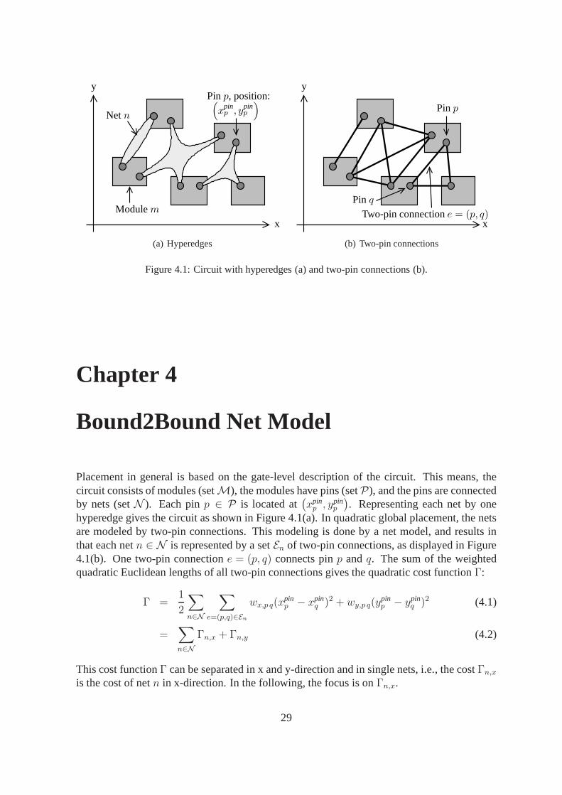
Netn
y
x
(
xpinp , ypin
p
)Pinp, position:
Modulem
(a) Hyperedges
y
x
Pin q
Two-pin connectione = (p, q)
Pinp
(b) Two-pin connections
Figure 4.1: Circuit with hyperedges (a) and two-pin connections (b).
Chapter 4
Bound2Bound Net Model
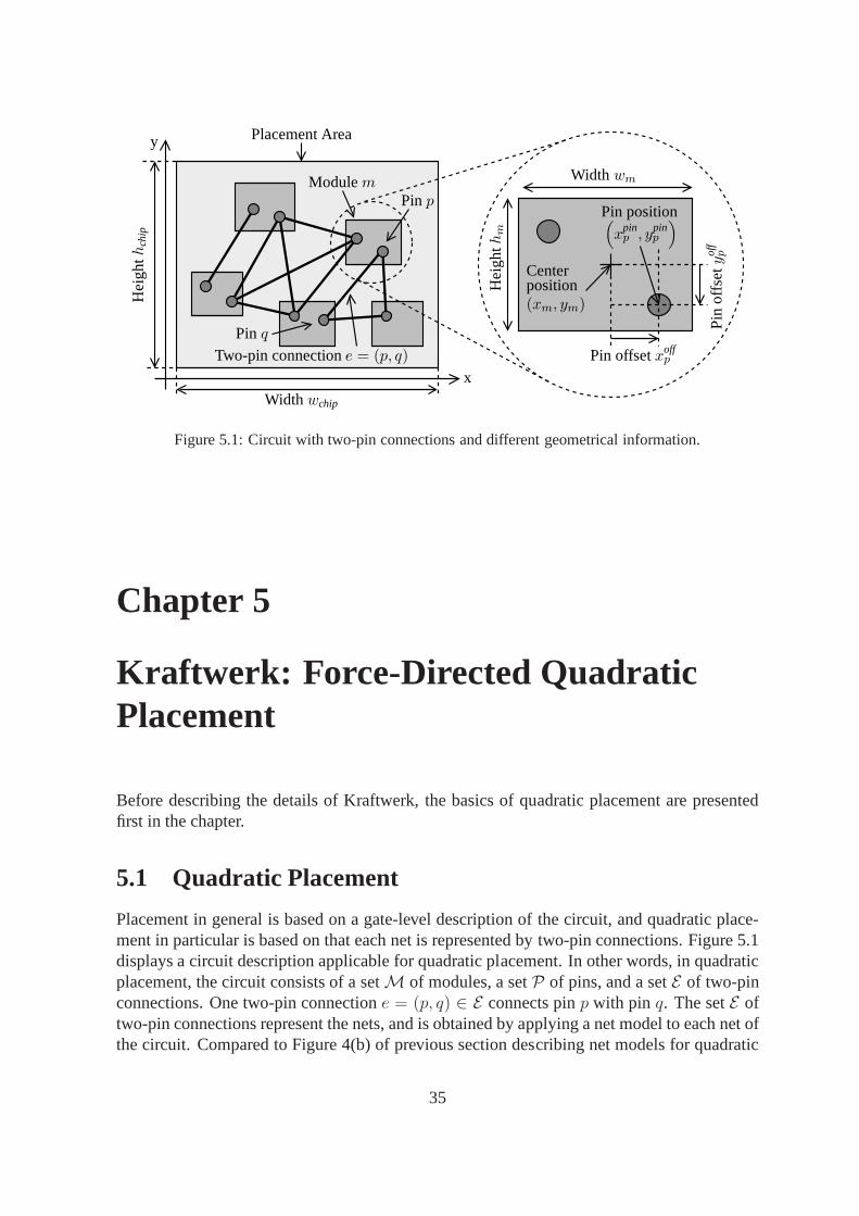
Placement in general is based on the gate-level descriptionof the circuit. This means, thecircuit consists of modules (setM), the modules have pins (setP), and the pins are connectedby nets (setN ). Each pinp ∈ P is located at
(xpin
p , ypinp
). Representing each net by one
hyperedge gives the circuit as shown in Figure 4.1(a). In quadratic global placement, the netsare modeled by two-pin connections. This modeling is done bya net model, and results inthat each netn ∈ N is represented by a setEn of two-pin connections, as displayed in Figure4.1(b). One two-pin connectione = (p, q) connects pinp andq. The sum of the weightedquadratic Euclidean lengths of all two-pin connections gives the quadratic cost functionΓ:
Γ =1
2
∑
n∈N
∑
e=(p,q)∈En
wx,p q(xpinp − xpin
q )2 + wy,p q(ypinp − ypin
q )2 (4.1)
=∑
n∈N
Γn,x + Γn,y (4.2)
This cost functionΓ can be separated in x and y-direction and in single nets, i.e., the costΓn,x
is the cost of netn in x-direction. In the following, the focus is onΓn,x.
29
30 CHAPTER 4. BOUND2BOUND NET MODEL
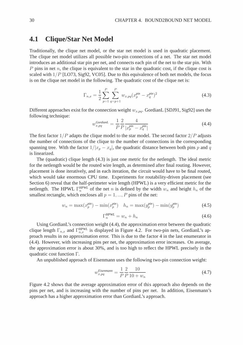
4.1 Clique/Star Net Model
Traditionally, the clique net model, or the star net model isused in quadratic placement.The clique net model utilizes all possible two-pin connections of a net. The star net modelintroduces an additional star pin per net, and connects eachpin of the net to the star pin. WithP pins in netn, the clique is equivalent to the star in the quadratic cost, if the clique cost isscaled with1/P [LO73, Sig92, VC05]. Due to this equivalence of both net models, the focusis on the clique net model in the following. The quadratic cost of the clique net is:
Γn,x =1
2
P∑
p=1
P∑
q=p+1
wx,pq(xpinp − xpin
q )2 (4.3)
Different approaches exist for the connection weightwx,pq. GordianL [SDJ91, Sig92] uses thefollowing technique:
wGordianLx,pq =
1
P
2
P
4
|xpinp − xpin
q |(4.4)
The first factor1/P adapts the clique model to the star model. The second factor2/P adjuststhe number of connections of the clique to the number of connections in the correspondingspanning tree. With the factor1/|xp − xq|, the quadratic distance between both pinsp andqis linearized.
The (quadratic) clique length (4.3) is just one metric for the netlength. The ideal metricfor the netlength would be the routed wire length, as determined after final routing. However,placement is done iteratively, and in each iteration, the circuit would have to be final routed,which would take enormous CPU time. Experiments for routability-driven placement (seeSection 6) reveal that the half-perimeter wire length (HPWL) is a very efficient metric for thenetlength. The HPWLΓHPWL
n of the netn is defined by the widthwn and heighthn of thesmallest rectangle, which encloses allp = 1, ..., P pins of the net:
wn = max(xpinp )−min(xpin
p ) hn = max(ypinp )−min(ypin
p ) (4.5)
ΓHPWLn = wn + hn (4.6)
Using GordianL’s connection weight (4.4), the approximation error between the quadraticclique lengthΓn,x andΓHPWL
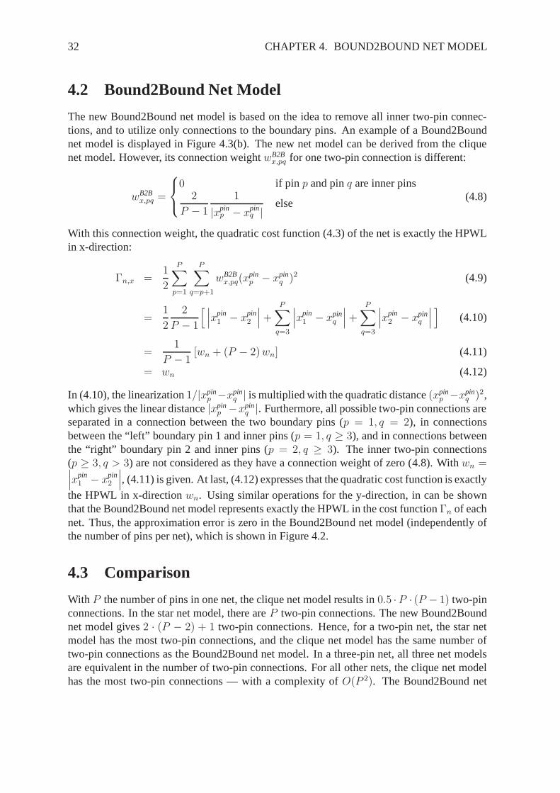
n,x is displayed in Figure 4.2. For two-pin nets, GordianL’s ap-proach results in no approximation error. This is due to the factor 4 in the last enumerator in(4.4). However, with increasing pins per net, the approximation error increases. On average,the approximation error is about 30%, and is too high to reflect the HPWL precisely in thequadratic cost functionΓ.
An unpublished approach of Eisenmann uses the following two-pin connection weight:
wEisenmannx,pq =
1
P
2
P
10
10 + wn
(4.7)
Figure 4.2 shows that the average approximation error of this approach also depends on thepins per net, and is increasing with the number of pins per net. In addition, Eisenmann’sapproach has a higher approximation error than GordianL’s approach.
4.1. CLIQUE/STAR NET MODEL 31
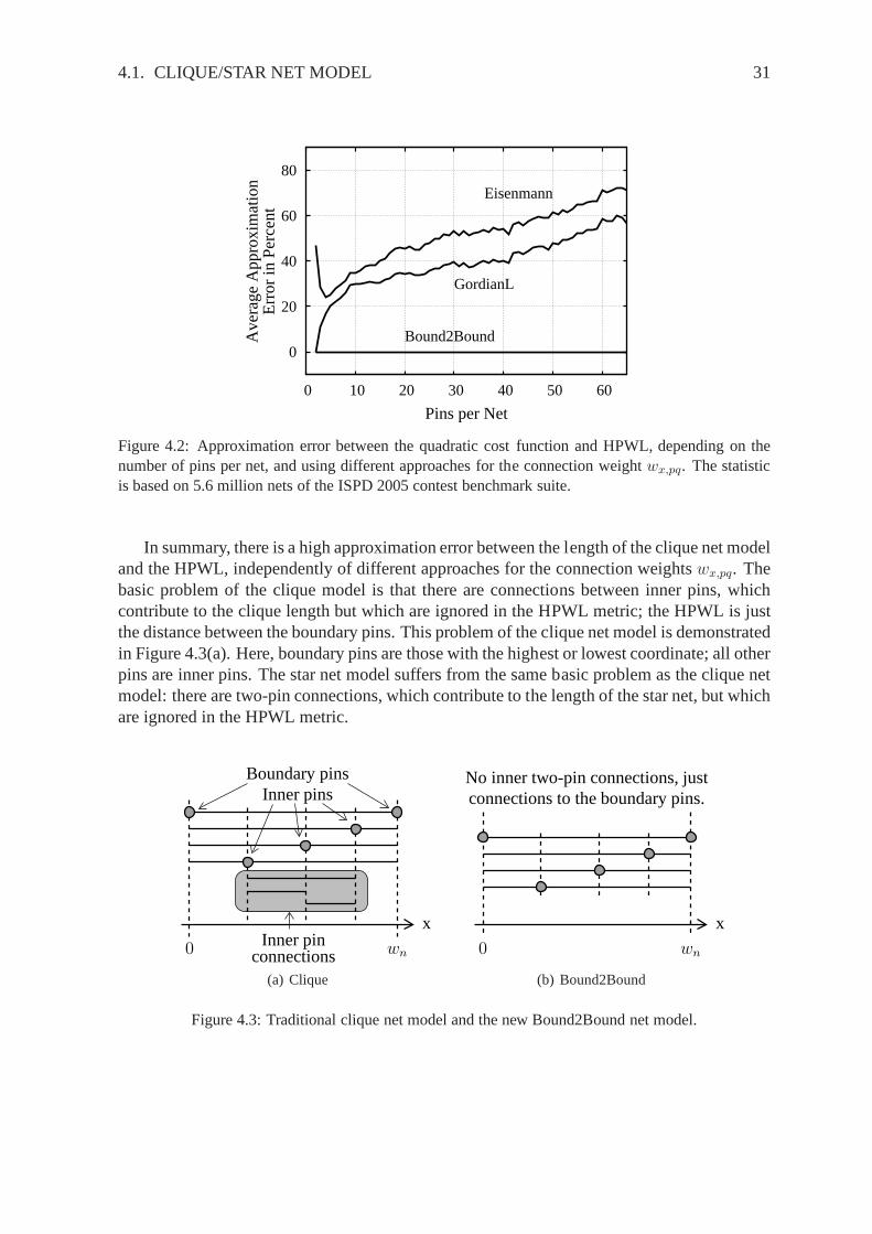
0
20
40
60
80
0 10 20 30 40 50 60
Ave
rage
App
roxi
mat
ion
Err
or in
Per
cent
Pins per Net
Bound2Bound
GordianL
Eisenmann
Figure 4.2: Approximation error between the quadratic costfunction and HPWL, depending on thenumber of pins per net, and using different approaches for the connection weightwx,pq. The statisticis based on 5.6 million nets of the ISPD 2005 contest benchmark suite.
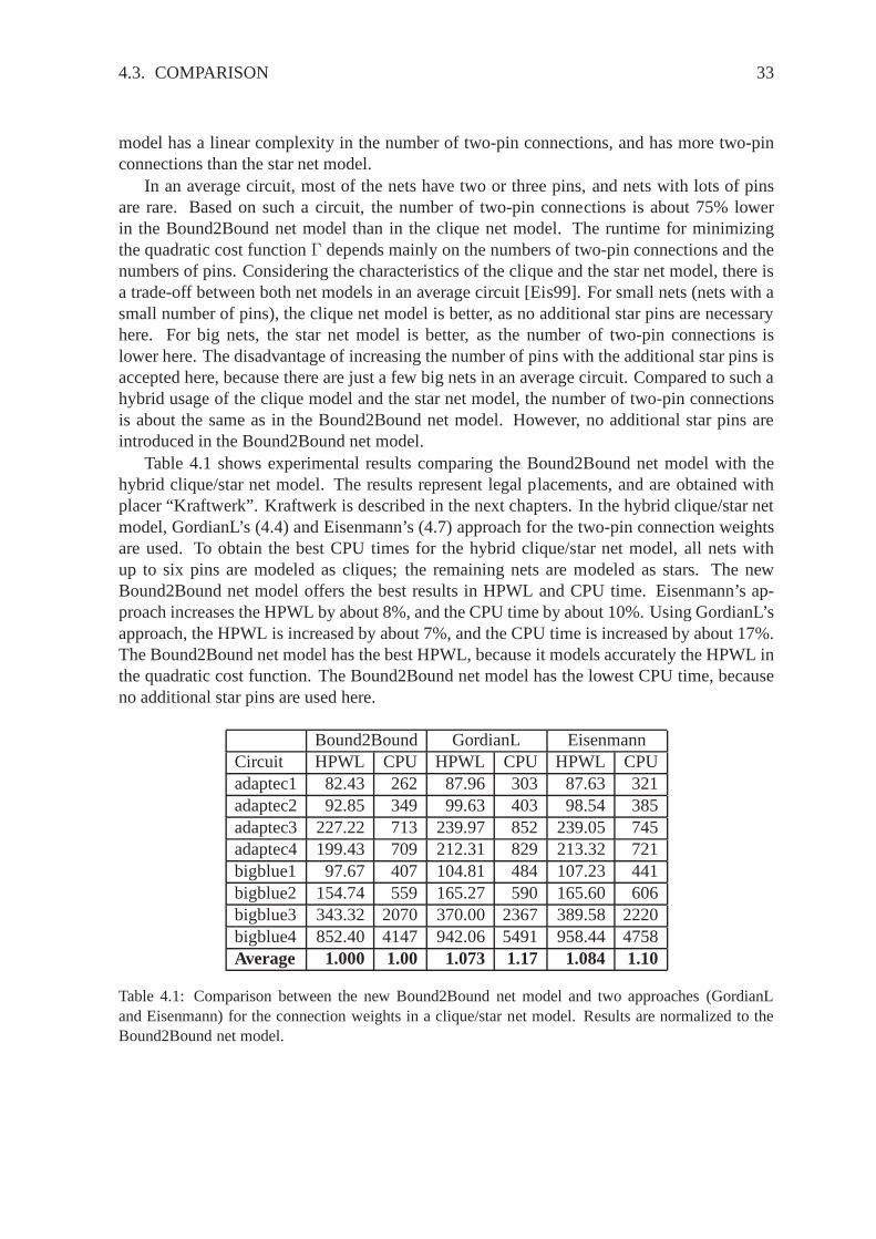
In summary, there is a high approximation error between the length of the clique net modeland the HPWL, independently of different approaches for theconnection weightswx,pq. Thebasic problem of the clique model is that there are connections between inner pins, whichcontribute to the clique length but which are ignored in the HPWL metric; the HPWL is justthe distance between the boundary pins. This problem of the clique net model is demonstratedin Figure 4.3(a). Here, boundary pins are those with the highest or lowest coordinate; all otherpins are inner pins. The star net model suffers from the same basic problem as the clique netmodel: there are two-pin connections, which contribute to the length of the star net, but whichare ignored in the HPWL metric.
wn0 Inner pinx
Inner pins
connections
Boundary pins
(a) Clique
wn0
x
connections to the boundary pins.No inner two-pin connections, just
(b) Bound2Bound
Figure 4.3: Traditional clique net model and the new Bound2Bound net model.
32 CHAPTER 4. BOUND2BOUND NET MODEL
4.2 Bound2Bound Net Model
The new Bound2Bound net model is based on the idea to remove all inner two-pin connec-tions, and to utilize only connections to the boundary pins.An example of a Bound2Boundnet model is displayed in Figure 4.3(b). The new net model canbe derived from the cliquenet model. However, its connection weightwB2B
x,pq for one two-pin connection is different:
wB2Bx,pq =
0 if pin p and pinq are inner pins2
P − 1
1
|xpinp − xpin
q |else
(4.8)
With this connection weight, the quadratic cost function (4.3) of the net is exactly the HPWLin x-direction:
Γn,x =1
2
P∑
p=1
P∑
q=p+1
wB2Bx,pq(x
pinp − xpin
q )2 (4.9)
=1
2
2
P − 1
[ ∣∣∣x
pin1 − xpin
2
∣∣∣ +
P∑
q=3
∣∣∣x
pin1 − xpin
q
∣∣∣ +
P∑
q=3
∣∣∣x
pin2 − xpin
q
∣∣∣
]
(4.10)
=1
P − 1[wn + (P − 2)wn] (4.11)
= wn (4.12)
In (4.10), the linearization1/|xpinp −xpin
q | is multiplied with the quadratic distance(xpinp −xpin
q )2,which gives the linear distance|xpin
p −xpinq |. Furthermore, all possible two-pin connections are
separated in a connection between the two boundary pins (p = 1, q = 2), in connectionsbetween the “left” boundary pin 1 and inner pins (p = 1, q ≥ 3), and in connections betweenthe “right” boundary pin 2 and inner pins (p = 2, q ≥ 3). The inner two-pin connections(p ≥ 3, q > 3) are not considered as they have a connection weight of zero (4.8). Withwn =∣∣∣x
pin1 − xpin
2
∣∣∣, (4.11) is given. At last, (4.12) expresses that the quadratic cost function is exactly
the HPWL in x-directionwn. Using similar operations for the y-direction, in can be shownthat the Bound2Bound net model represents exactly the HPWL in the cost functionΓn of eachnet. Thus, the approximation error is zero in the Bound2Bound net model (independently ofthe number of pins per net), which is shown in Figure 4.2.
4.3 Comparison
With P the number of pins in one net, the clique net model results in0.5 ·P · (P − 1) two-pinconnections. In the star net model, there areP two-pin connections. The new Bound2Boundnet model gives2 · (P − 2) + 1 two-pin connections. Hence, for a two-pin net, the star netmodel has the most two-pin connections, and the clique net model has the same number oftwo-pin connections as the Bound2Bound net model. In a three-pin net, all three net modelsare equivalent in the number of two-pin connections. For allother nets, the clique net modelhas the most two-pin connections — with a complexity ofO(P 2). The Bound2Bound net
4.3. COMPARISON 33
model has a linear complexity in the number of two-pin connections, and has more two-pinconnections than the star net model.
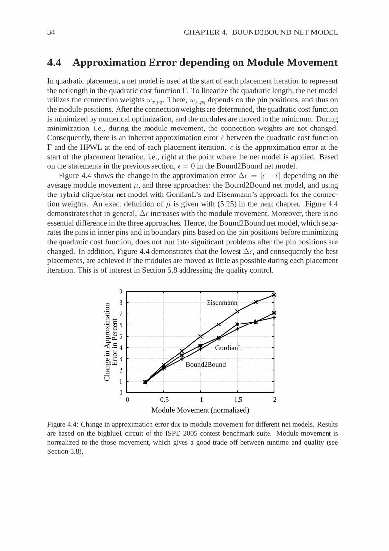
In an average circuit, most of the nets have two or three pins,and nets with lots of pinsare rare. Based on such a circuit, the number of two-pin connections is about 75% lowerin the Bound2Bound net model than in the clique net model. Theruntime for minimizingthe quadratic cost functionΓ depends mainly on the numbers of two-pin connections and thenumbers of pins. Considering the characteristics of the clique and the star net model, there isa trade-off between both net models in an average circuit [Eis99]. For small nets (nets with asmall number of pins), the clique net model is better, as no additional star pins are necessaryhere. For big nets, the star net model is better, as the numberof two-pin connections islower here. The disadvantage of increasing the number of pins with the additional star pins isaccepted here, because there are just a few big nets in an average circuit. Compared to such ahybrid usage of the clique model and the star net model, the number of two-pin connectionsis about the same as in the Bound2Bound net model. However, noadditional star pins areintroduced in the Bound2Bound net model.
Table 4.1 shows experimental results comparing the Bound2Bound net model with thehybrid clique/star net model. The results represent legal placements, and are obtained withplacer “Kraftwerk”. Kraftwerk is described in the next chapters. In the hybrid clique/star netmodel, GordianL’s (4.4) and Eisenmann’s (4.7) approach forthe two-pin connection weightsare used. To obtain the best CPU times for the hybrid clique/star net model, all nets withup to six pins are modeled as cliques; the remaining nets are modeled as stars. The newBound2Bound net model offers the best results in HPWL and CPUtime. Eisenmann’s ap-proach increases the HPWL by about 8%, and the CPU time by about 10%. Using GordianL’sapproach, the HPWL is increased by about 7%, and the CPU time is increased by about 17%.The Bound2Bound net model has the best HPWL, because it models accurately the HPWL inthe quadratic cost function. The Bound2Bound net model has the lowest CPU time, becauseno additional star pins are used here.
Table 4.1: Comparison between the new Bound2Bound net modeland two approaches (GordianLand Eisenmann) for the connection weights in a clique/star net model. Results are normalized to theBound2Bound net model.
34 CHAPTER 4. BOUND2BOUND NET MODEL
4.4 Approximation Error depending on Module Movement
In quadratic placement, a net model is used at the start of each placement iteration to representthe netlength in the quadratic cost functionΓ. To linearize the quadratic length, the net modelutilizes the connection weightswx,pq. There,wx,pq depends on the pin positions, and thus onthe module positions. After the connection weights are determined, the quadratic cost functionis minimized by numerical optimization, and the modules aremoved to the minimum. Duringminimization, i.e., during the module movement, the connection weights are not changed.Consequently, there is an inherent approximation errorǫ between the quadratic cost functionΓ and the HPWL at the end of each placement iteration.ǫ is the approximation error at thestart of the placement iteration, i.e., right at the point where the net model is applied. Basedon the statements in the previous section,ǫ = 0 in the Bound2Bound net model.
Figure 4.4 shows the change in the approximation error∆ǫ = |ǫ − ǫ| depending on theaverage module movementµ, and three approaches: the Bound2Bound net model, and usingthe hybrid clique/star net model with GordianL’s and Eisenmann’s approach for the connec-tion weights. An exact definition ofµ is given with (5.25) in the next chapter. Figure 4.4demonstrates that in general,∆ǫ increases with the module movement. Moreover, there is noessential difference in the three approaches. Hence, the Bound2Bound net model, which sepa-rates the pins in inner pins and in boundary pins based on the pin positions before minimizingthe quadratic cost function, does not run into significant problems after the pin positions arechanged. In addition, Figure 4.4 demonstrates that the lowest ∆ǫ, and consequently the bestplacements, are achieved if the modules are moved as little as possible during each placementiteration. This is of interest in Section 5.8 addressing thequality control.
0
1
2
3
4
5
6
7
8
9
0 0.5 1 1.5 2
Cha
nge
in A
ppro
xim
atio
nE
rror
in P
erce
nt
Module Movement (normalized)
Bound2Bound
GordianL
Eisenmann
Figure 4.4: Change in approximation error due to module movement for different net models. Resultsare based on the bigblue1 circuit of the ISPD 2005 contest benchmark suite. Module movement isnormalized to the those movement, which gives a good trade-off between runtime and quality (seeSection 5.8).
Modulem
Two-pin connectione = (p, q)
Pin
offs
ety
off
p
Pin offsetxoffp
Width wchip
He
igh
thch
ip
x
y Placement Area
He
igh
thm
Width wm
(xm, ym)positionCenter
Pin position
Pin q
(
xpinp , ypin
p
)
Pinp
Figure 5.1: Circuit with two-pin connections and differentgeometrical information.
Chapter 5
Kraftwerk: Force-Directed QuadraticPlacement
Before describing the details of Kraftwerk, the basics of quadratic placement are presentedfirst in the chapter.
5.1 Quadratic Placement
Placement in general is based on a gate-level description ofthe circuit, and quadratic place-ment in particular is based on that each net is represented bytwo-pin connections. Figure 5.1displays a circuit description applicable for quadratic placement. In other words, in quadraticplacement, the circuit consists of a setM of modules, a setP of pins, and a setE of two-pinconnections. One two-pin connectione = (p, q) ∈ E connects pinp with pin q. The setE oftwo-pin connections represent the nets, and is obtained by applying a net model to each net ofthe circuit. Compared to Figure 4(b) of previous section describing net models for quadratic
placement, the figure above displays additional geometric information necessary for place-ment. So, modulem ∈ M is characterized by its widthwm, its heighthm, and its centerposition(xm, ym). The placement area, i.e., the chip area, is described by itswidth wchip andits heighthchip. Similar to previous section, pinp ∈ P is located at position(xpin
p , ypinp ).
In quadratic placement, the length of all nets is represented in the quadratic cost functionΓ, the sum of the weighted quadratic Euclidean lengths of all two-pin connections:
Γ =1
2
∑
e=(p,q)∈E
wx,pq(xpinp − xpin
q )2 + wy,pq(ypinp − ypin
q )2 (5.1)
Placement determines the positions of all modules, such that the netlength is minimal.In quadratic placement, the quadratic cost functionΓ is minimized. However,Γ depends in(5.1) on the pin positions, and not on the module positions. Hence, a transformation from pinposition to module position is necessary. To do this transformation, the functionπ(p) = mmaps the pinp ∈ P to the modulem ∈ M, according to the relation between modulem andpin p:
π : P →M π(p) = m: pin p ∈ P belongs to modulem ∈M (5.2)
The pin offset(xoffp , yoff
p ) (see Figure 5.1) describes the difference between the module positionand the pin position:
xoffp = xpin
p − xm yoffp = ypin
p − ym (5.3)
Using (5.2) and (5.3), the pin position is described by the pin offset and the correspondingmodule position:
xpinp = xπ(p) − xoff
p ypinp = yπ(p) − yoff
p (5.4)
Placement also separates the modules in movable and fixed ones, because only the positionsof the movable modules have to be determined by placement. The positions of theM movablemodules are represented in vectorx for x-direction, and in vectory for y-direction:
x = (x1, x2, x3, ..., xM)T (5.5)
y = (y1, y2, y3, ..., yM)T (5.6)
Using (5.2), (5.4), (5.5), and (5.6), the quadratic cost functionΓ represented as a sum in (5.1),can be transformed in a matrix-vector notation:
Γ =1
2xTCxx + xTdx +
1
2yTCyy + yTdy + const (5.7)
MatricesCx andCy represent the connectivity between movable modules, and vectorsdx
anddy reflect the connections between movable and fixed modules. Detailed steps to createthe matrices and the vectors are described later on. If thereare no modules fixed, matricesCx
andCy are positive semidefinite [Hal70]. With some modules fixed, the matrices are positivedefinite [KV06]. In both cases,Γ is convex, and its minimum is obtained by setting its firstderivative to zero. The first derivatives in x- and in y-direction are described by the nabla
5.2. CREATION OF MATRIXCX AND VECTORDX 37
operators∇x and∇y:
∇x =
(∂
∂x1,
∂
∂x2, ...,
∂
∂xM
)T
(5.8)
∇y =
(∂
∂y1,
∂
∂y2, ...,
∂
∂yM
)T
(5.9)
Using these nabla operators, the derivatives ofΓ in x- and y-direction are given:
∇xΓ = Cxx + dx (5.10)
∇yΓ = Cyy + dy (5.11)
Setting these derivatives to zero gives two systems of linear equations:
Cxx + dx = 0 (5.12)
Cyy + dy = 0 (5.13)
Solving these systems with respect tox andy gives the module positionsx andy with min-imal netlength. (5.12) and (5.13) demonstrate thatx andy are determined separately. More-over, both directions (x and y) or obtained similarly. Hence, the focus is on the x-direction inthe following. The y-direction is obtained analogously.
5.2 Creation of Matrix Cx and Vector dx
This section describes how matrixCx and vectordx of the quadratic cost functionΓ (5.7)are created. Using (5.2) and (5.3), the cost function in x-directionΓx can be written in sumnotation, depending on the module positionsxi, i = 1, 2, ..., M + F . M is the number ofmovable modules, andF the number of fixed modules.
Γx =1
2
∑
e=(p,q)∈E
wx,pq(xπ(p) − xoffp − xπ(q) + xoff
q )2 (5.14)
The cost of one two-pin connection is given by:
Γx,pq =wx,pq
2
(xπ(p) − xoff
p − xπ(q) + xoffq
)2(5.15)
With this cost, the sum notation of (5.14) can be rewritten:
Vectorx represents the x-position of theM movable modules (5.5). MatrixCx = [cx,ij] is atwo-dimensional matrix withM rows andM columns.cx,ij is the entry ofCx in row i andcolumnj. Vectordx = [dx,i] is a column vector withM entries.dx,i is the entry ofdx in rowi.
The creation ofCx and vectordx is described at best by using the derivative ofΓx:
∇xΓx = Cxx + dx (5.18)
A small part of the system of linear equation (5.18) looks like:
...∂
∂xi
...∂
∂xj
...
Γx =
......
......
.... . . cx,ii . . . cx,ij . . ....
.... . .
......
. . . cx,ji . . . cx,jj . . ....
......
......
...xi
...xj
...
+
...dx,i
...dx,j
...
(5.19)
The i-th row in this system of linear equations (5.19) represents the derivative ofΓx withrespect toxi. In the sum notation (5.16), this derivative is:
∂
∂xi
Γx =∑
e=(p,q)∈E
∂
∂xi
Γx,pq (5.20)
Depending oni, p, andq, the derivative of the cost ofΓx,pq of one two-pin connectione =(p, q) is:
∂
∂xi
Γx,pq =
wx,pq(xi − xoffp − xπ(q) + xoff
q ) if i = π(p)
−wx,pq(xπ(q) − xoffp − xi + xoff
q ) if i = π(q)
0 else
(5.21)
Using all of this, the contribution of one two-pin connection e = (p, q) to the matrixCx andvectordx is as follows (with the substitutioni = π(p) andj = π(q)):
1. i, j ≤ M , which means that both modulesi andj are movable.The diagonal entriescx,ii and cx,jj of the matrix are increased bywx,pq, and the off-diagonal entriescx,ij andcx,ji are decreased bywx,pq. The entrydx,i of vectordx isincreased bywx,pq(−xoff
p + xoffq ), and the entrydx,j is decreased bywx,pq(−xoff
p + xoffq ).
2. i ≤M ∧ j > M , which means that modulei is movable andj is fixed.The entrycx,ii of the matrixCx is increased bywx,pq. In the vectordx, the entrydx,i isincreased bywx,pq(−xoff
p − xπ(q) + xoffq ).
3. i > M ∧ j ≤ M , which means that modulei is fixed andj is movable.The entrycx,jj of the matrixCx is increased bywx,pq. In the vectordx, the entrydx,j isdecreased bywx,pq(xπ(p) − xoff
p + xoffq ).
4. i > M ∧ j > M , which means that both modulesi andj are fixed.Matrix Cx and vectordx do not change.
5.3. FORCE-DIRECTED QUADRATIC PLACEMENT 39
To create matrixCx and vectordx, both are initialized with zeros first. Then, the contri-bution of each two-pin connectione ∈ E , as described above, is considered inCx anddx.This gives the matrixCx and the vectordx.
Based on the creation of the matrixCx, different properties ofCx can be deduced:
1. The matrixCx is symmetric.
2. The diagonal entries of matrixCx are all non-zeros, and are all positive.
3. The off-diagonal entries of matrixCx are mostly zeros, and if not, they are negative.
4. The matrix is weak diagonal dominant, i.e., for alli = 1, ..., N :N∑
j=1∧j 6=i
|cx,ij| ≤ |cx,ii|.
5. Using the Bound2Bound net model, the number of non-zeros depends about linearlyon the number of movable modulesN . Hence, the matrixCx is highly sparse. Thisproperty was analyzed using different circuits of various benchmark suites.
Because of these properties, the system of linear equation (5.12) can be solved very effi-ciently by numerical approaches, e.g., with the conjugate-gradient approach [You03]. Thus,the module positions are determined in low runtime, which isa main advantage of quadraticplacement, compared to other placement approaches like non-linear placement or min-cutplacement. Details of solving a system of linear equations are presented in Section 5.12.2.
5.3 Force-directed Quadratic Placement
In quadratic placement, the costΓx,pq (5.15) of one two-pin connectione = (p, q) can beinterpreted as the energy of an elastic spring, which is spanned between both pinsp andq. Inother words, each two-pin connection corresponds to one spring. All two-pin connections ofone circuit create a spring system, whose total energy is thequadratic cost functionΓx (5.16).Since the derivative of the energy with respect to x (or y) is the force in x (or y) direction, thederivative ofΓx is called the “net” force:
Fnetx = ∇xΓx = Cxx + dx (5.22)
The name “net” force is because this force is created by the two-pin connections, and thetwo-pin connections represent the nets. The net force is setto zero in (5.12) and (5.23), toobtain the equilibrium state of the spring system, i.e., thestate with minimal energy. Thiscorresponds to the placement with minimal netlength.
Fnetx = 0 (5.23)
With just the net force acting on the modules, the modules arestrongly attracted, whichresults in a lot of module overlap. Mostly, the modules are concentrated in the center of thechip. This is displayed in Figure 5.2 (a). Force-directed quadratic placers utilize an additionalforce to spread the modules on the chip, and this is done in a sequence of placement iterations.Two placement iterations are shown in Figure 5.2 (b) and (c).
Figure 5.2: Placement with minimal netlength (a), and placements at certain placement iterations (b)and (c). In each placement iteration, forces are applied to move the modules and to reduce the overlap.
Previous sections described quadratic placement in general. The following sections presentsthe novel force-directed quadratic placement approach called “Kraftwerk”. Kraftwerk is basedon separating the additional force into two fundamental forces, and both forces are imple-mented in a systematic way. The result of Kraftwerk’s systematic force implementation isan advanced convergence for various circuits, even for hardinstances of macro cell circuits,where the placement area provides only few free space. In other words, Kraftwerk can placemany different, and sometimes challenging circuits. Thus,it is a robust placer. Later on, theconvergence will be analyzed in theory and based on experimental results. Since Kraftwerkneeds only a few placement iterations to spread the modules on the placement area, Kraftwerkis a fast placer.
5.4 Geometry
Before going into details on Kraftwerk’s force implementation, some geometric properties aredescribed now. They are of interest, because they are used frequently in the remaining thesis.The geometric properties of onei module is shown in Table 5.1.
(x′i, y
′i) Position at the start of a placement iteration
(xi, yi) Position at the end of a placement iteration(∆xi, ∆yi) Change of the position∆xi = xi − x′
i ∆yi = yi − y′i
wi, hi Width, heightAmod,i = wi · hi Areadmod,i Individual density, used in the module demand
Table 5.1: Properties of one modulei. Position means the center position of the module.
5.4. GEOMETRY 41
The total module areaAmod,tot is the sum of the areas of allM movable andF fixed modules.
Amod,tot=
M+F∑
i=1
Amod,i (5.24)
The average module movementµ is:
µ =1
M
M∑
i=1
∣∣(∆xi, ∆yi)
T∣∣ (5.25)
Here,| · |means the Euclidean norm.Table 5.2 summarizes the geometric properties of the chip. Here, it should be noted that
the term “chip” and “placement area” are used interchangeably in this thesis.
(xchip, ychip) Position of the lower left cornerwchip, hchip Width, heightAchip = wchip · hchip Area
Table 5.2: Properties of the chip.
In the tables above, it is assumed implicitly that the modules and the chip are rectangular.This is done for simplicity. However, in Kraftwerk, the modules and the chip can have anyshape, even circles are possible. Assuming rectangular structure, a rectangle functionR issuitable to represent the modules and the chip in the two-dimensional space x-y.R is one forall points(x, y) within a rectangle, and zero outside. The rectangle is defined by its lower leftcorner(xll, yll), its widthw, and its heighth.
R(x, y; xll, yll, w, h) =
1 if 0 ≤ x− xll ≤ w ∧ 0 ≤ y − yll ≤ h
0 else(5.26)
The rectangle functionR can be used to compute different geometrical properties. So, amodule distributionV (x, y) is defined by:
V (x, y) =M+F∑
i=1
R(x, y; x′
i − wi
2, y′
i − hi
2, wi, hi
)(5.27)
V reflects at point(x, y) the number of module rectangles covering this point. Hence,V (x, y)is the “local module density” at point(x, y). In contrast to this, the term “module density”means the ratio between the total module areaAmod,totand the placement areaAchip. The term“module overlap”Ω represents the areaA∪ of the union of all modules, normalized to thetotal areaAmod,totof all modules:
A∪ is determined similar to Klee’s measure problem in two dimensions [Kle77]. Based onV (x, y), the areaA∪ of the unions of all modules is calculated by:
A∪ =
∞∫
−∞
∞∫
−∞
ω(x, y) dx dy with ω(x, y) =
1 if V (x, y) ≥ 1
0 else(5.29)
If there is no overlap between the modules, thenA∪ = Amod,tot, andΩ = 0. If the circuitconsists of a high number of modules, all of which are small indimension and are concentratedsomewhere on the chip, thenA∪ ≪ Amod,tot, andΩ ≈ 1.
5.5 One Placement Iteration
Based on one placement iteration, the systematic force implementation of Kraftwerk is de-scribed in the following. First, a formal description is given, and then an illustration of theforces is presented. The module positions in each placementiteration are denoted as follows:the vectorx′ represents the starting positions, the vectorx represents the new positions, andthe vector∆x is the change of position:
∆x = x− x′ (5.30)
5.5.1 Move Force
The move force moves the modules in the current placement iteration, in order to reduce themodule overlap, and to spread the modules over the chip. To determine the move force, theplacement is represented in generic demand-and-supply systemD. In principle, the modulescreate the demandDdem, and the placement area creates the supplyDsup.
D(x, y) = Ddem(x, y)−Dsup(x, y) (5.31)
The demand-and-supply system has to be balanced, i.e., the integral over the demand has toequal the integral over the supply. This is necessary to adapt the demand completely to thesupply.
∞∫
−∞
∞∫
−∞
Ddem(x, y) dx dy =
∞∫
−∞
∞∫
−∞
Dsup(x, y) dx dy (5.32)
Using the rectangle functionR (5.26), the demand of one modulei is:
D demmod,i(x, y) = dmod,i ·R
(x, y; x′
i − wi
2, y′
i − hi
2, wi, hi
)(5.33)
The module demandD demmod for all M movable andF fixed modules is the sum of all single
module demandsD demmod,i:
D demmod (x, y) =
M+F∑
i=1
D demmod,i(x, y) (5.34)
5.5. ONE PLACEMENT ITERATION 43
For simplicity, the individual module densitydmod,i is set to one here. Hence, there is no dif-ference between the module demandD dem
mod (x, y) and the module distributionV (x, y) (5.27).Section 5.10 presents an advanced approach for scalingdmod,i, in order to remove unwantedhalos around large each modules. Here, “halo” means free space (see Figure 5.7). In themodule demand (5.34), there is no fundamental difference between small or large modules,or between fixed or movable modules. Thus, it can be used to place various circuit types likestandard-cell circuits with millions of small modules, mixed-size circuits with small and bigmodules, and circuits with fixed modules.
Besides a module demand, a module supplyD supmod is necessary for the demand-and-supply
system. In the simplest case, the whole placement area provides supply for the modules:
The module supply densitydsup is determined by (5.34) and (5.32):
dsup =
M+F∑
i=1
dmod,i Amod,i
Achip(5.36)
Using (5.35), the modules are spread over the whole placement area. Section 5.11 presentsan advanced approach for the module supply, in order to spread the modules according to auser-given module density. With this, the modules are not spread over the whole placementarea, but can be placed tightly, which reduces the netlength.
The module demand-and-supply systemDmod is the module demandD demmod minus the mod-
ule supplyD supmod:
Dmod(x, y) = D demmod (x, y)−D sup
mod(x, y) = D(x, y) (5.37)
To place the modules overlap-free on the chip, the module demand-and-supply system is usedfor D. However, the generic demand-and-supply systemD can be extended by additionaldemand-and-supply systems. For example, it can be extendedby the routing demand-and-supply system, in order to optimize routability during placement. This is described in Section6.4.D can also be used to optimize the temperature profile of a chip [OJ04b, Obe05].
The generic demand-and-supply systemD (5.31), and thus the module demand-and-supply systemDmod (5.37), is interpreted as a charge distribution, and the charge distributioncreates an electrostatic potentialΦ by Poisson’s equation:
(∂2
∂x2+
∂2
∂y2
)
Φ(x, y) = −D(x, y) (5.38)
Section 5.12.1 gives details on computing the potentialΦ. The usage of a potential is similar toEisenmann’s placement approach [EJ98, Eis99, Obe05]. However, there, a “constant” force isused, and the force is accumulated over the placement iterations. In contrast to this, Kraftwerk,as presented in this thesis, models the move force with target points and spring connections.Consequently, the move force depends onx, and is not a constant force. In addition, a holdforce is used in Kraftwerk, in order to decouple each placement iteration from the previous
one. Consequently, no force accumulation is necessary. As aresult of this new force modeling,the placement algorithm has an advanced convergence. Section 5.9 analyzes the convergenceof Kraftwerk in theory and based on experimental results.
Back to the move force. For modulei, this forceF movex,i is created by a spring connection
between the module and its target pointxi.
F movex,i = wi (xi − xi) (5.39)
The target pointxi is determined by the starting module positionx′i and the negative gradient
of the potentialΦ.
xi = x′i −
∂
∂xΦ(x, y)
∣∣∣(x′
i,y′
i)(5.40)
Based on the move force, which depends via the target point onthe potentialΦ (5.39) and(5.40), and the potential represents the demand-and-supply systemD (5.38), Kraftwerk isdriven by adapting the demand-and-supply systemD. wi in (5.39) is the spring constant ofthe move force, and is denoted also as the weight of the move force. wi affects the distance amodulei is moved during one placement iteration: with a highwi, the move force of modulei pulls a lot on its module, and the module will be moved a long distance. The opposite is truefor a smallwi. Using target points for the move force, the modules can be moved at most upto their target point during one placement iteration. Hence, the module movement is limited.Moreover, the movement limit is decreasing continuously over the placement iterations. All ofthis enforces Kraftwerk’s convergence. To represent the move force (5.39) in a matrix-vectornotation, the weights of the move force are collected in the diagonal matrixCx:
Cx = diag(wi) (5.41)
The gradients of the potential are collected in the vectorΦx:
Φx =
(∂
∂xΦ
∣∣∣(x′
1,y′
1),
∂
∂xΦ
∣∣∣(x′
2,y′
2), ...,
∂
∂xΦ
∣∣∣(x′
M,y′
M)
)T
(5.42)
All target points are represented in the vectorx = x′ −Φx. Therefore, the move forceFmovex
in matrix-vector notation is:Fmove
x = Cx (x− x) (5.43)
5.5.2 Hold Force
To spread the modules iteratively on the chip, the move forceis used. However, besides themove force, the net force is acting on the modules to minimizethe netlength. Thus, the netforce has to be compensated at the start of each placement iteration. Otherwise, the modulescollapse back to the initial placement, where the netlengthis minimal, but the modules overlapa lot. The compensation of the net force is done by the hold force, and the hold forceFhold
x
equals the negative net force:Fhold
x = − (Cxx′ + dx) (5.44)
5.5. ONE PLACEMENT ITERATION 45
Using only the hold force as one additional force, the modules will not collapse back, butstay at their position in the current placement iteration. In other words, the change in moduleposition∆x is zero. This can be shown by:Fnet
x + Fholdx = 0⇔ Cx∆x = 0 ⇔ ∆x = 0. It
should be noted here that the hold force equals the net force only at the start of the placementiteration, where the modules are located atx′. Moreover, the hold force is a constant force, asit does not depend onx.
The result of the hold force is that each placement iterationis decoupled from the previousone. Therefore, the placement algorithm can be restarted atany iteration, and the engineeringchange order (ECO) is supported best. For example, after gate sizing the circuit, and thusintroducing module overlap, the placement process can be restarted from the last placement,in order to remove the introduced module overlap. Hence, theplacement process needs not bestarted from scratch, which saves a lot of runtime. Section 8.2 presents experimental resultsof the ECO feature of Kraftwerk.
Figure 5.3: Illustration of one placement iteration. The numbers in the big arrows represent the se-quence of the steps, taken in each placement iteration. (a) Given placement with modules and nets.(b) Hold force to preserve the placement of (a). (d) Demand-and-supply system. (e) Potential. (d) and(e) are density plots with white color representing low density and black color high density. (f) Moveforce, created by springs between the modules and their target points. (c) Resulting placement (sum ofthe net, move, and hold force is zero). The target points are represented by crosses in (c) and (f).
Previous sections described in a formal way how the move force and the hold force are de-termined, and how they are modeled. This section presents anillustration of one placementiteration, particularly of the forces.
The placement iteration starts with a given placement, where each modulei is located at(x′
i, y′i). Figure 5.3 (a) displays such a placement. Ignoring the moveforce, only the net force
is acting on the modules and attracts them together. To compensate for this, the hold force isused, which preserves the given placement. The hold forces are displayed as arrows in Figure5.3(b).
Based on the module positions, the demand-and-supplyD system is created, which repre-sents the local module density. Figure 5.3 (d) showsD of the given placement.D is treated asa charge distribution, which creates an electrostatic potential Φ via Poisson’s equation. Sucha potential is displayed in Figure 5.3(e). ComparingD in Figure 5.3 (d) with the potentialΦin Figure 5.3 (e) reveals that the potentialΦ can be viewed as a smoothed representation ofthe demand-and-supply systemD. Moreover, in regions whereD is low, the potentialΦ islow, and vice versa.
The gradients of the potential, evaluated at the positions of the modules, determine thetarget points. The target points are displayed as crosses inFigure 5.3(e). The move force iscreated by spring connections between the modules and theirtarget points. With the springsto the target points, the modules are moved away from high density regions (black regions in5.3(d) and (e)) towards low density regions (white regions in 5.3(d) and (e)).
Hence, three forces are acting on the modules in each placement iteration: the net force,the hold force, and the move force. These forces move the modules, until the sum of the forcesis zero. The placement, where the sum of all three forces is zero, is the resulting placementof one placement iteration. Figure 5.3(f) displays the resulting placement. Comparing Figure5.3(c) with (f) shows that the modules are moved towards the target points. In addition, themodules are spread more over the placement area, and the module overlap is reduced.
5.6 Core of Kraftwerk
In summary, three forces are used by Kraftwerk in each placement iteration: the net forceFnet
x , and two additional forces: the move forceFmovex and the hold forceFhold
x . Setting thesum of the three forces to zero (5.45) gives the core system oflinear equations (5.46) used inKraftwerk’s iterative placement process.
Fnetx + Fmove
x + Fholdx = 0 (5.45)
(
Cx + Cx
)
∆x = −CxΦx (5.46)
Solving (5.46) with respect to∆x, and updatingx′ by ∆x gives the new module positionsxin the current placement iteration. Details on solving (5.46) are described in Section 5.12.2.Based on (5.46), Kraftwerk has three degrees of freedom. First, the cost functionΓ, rep-resented inCx. Second, the demand-and-supply systemD, represented inΦx. Third, the
5.7. OVERVIEW OF THE PLACEMENT ALGORITHM 47
weights of the move forcewi, represented inCx. Kraftwerk is very flexible and utilizes thedegrees of freedom to optimize different objectives (like HPWL netlength and routability),and to control the quality of placement.
5.7 Overview of the Placement Algorithm
Algorithm 1 : Global placement algorithm “Kraftwerk”.
// Start with given placementwhile Module overlapΩ ≥ 20% do1
Determine demand-and-supply systemD(x, y);2
Calculate potentialΦ(x, y) based onD(x, y) and Poisson’s equation (5.38);3
Apply net model;4
// In x-direction (similarly in y-direction):begin5
CreateCx, Cx, andΦx;6
Solve(
Cx + Cx
)
∆x = −CxΦx w.r.t. ∆x;7
Update module positionsx by ∆x;8
end9
Call quality control;10
end11
// Next step: final placement (legalization and detailed placement)
Algorithm 1 displays the iterative global placement algorithm of Kraftwerk. The globalplacement starts with a given placement. This can be a placement of a previous run ofKraftwerk, but with additional module overlap introduced,e.g., after gate sizing the placedcircuit. Or, the placement is run from scratch, i.e., it is started with the initial placement. Forthe initial placement, all modules are placed at the center of the chip, and the quadratic costfunctionΓ (5.7) is minimized over a few iterations (about five). In eachiteration, a net modelis applied to represent the netlength inΓ.
In global placement, the modules are spread iteratively on the chip. Each placement iter-ation starts with determining the demand-and-supply system D (line 2), and computing thepotentialΦ (line 3). Then a net model is applied to determine the weightsof the two-pinconnections and to represent the netlength in the quadraticcost functionΓ (line 4). After that,all elements of the core system of linear equations (5.46) are determined (line 6). Then, (5.46)is solved with respect to∆x (line 7), and the module positions are updated (line 8). Thesethree steps (line 6-8) are done for x- and y-direction. At theend of each placement iteration,a quality control procedure is called, in order to adjust theweights of the move force. Theglobal placement is stopped if the module overlapΩ (5.28) is below a certain limit, e.g., below20%.
After global placement, final placement is done. Here, the modules are legalized first,which means that the remaining overlap is removed, and the modules are aligned to rows/grid
structure if necessary. Considering the remaining overlapof about 20%, the legal placementis obtained quickly (about 5% of the runtime of global placement), and the netlength increaseby about 1%. Chapter 7 presents new approaches for legalization. After legalization, detailedplacement can be used to improve the legal placement.
5.8 Quality Control
The weightswi (i = 1, 2, 3, ..., M) of the move force (5.41) are one degree of freedom ofKraftwerk. They are utilized to control the iterative global placement process, and to controlthe quality of placement. The weightwi of modulei is initialized at the beginning of theglobal placement process according to:
wi =Amod,i
Aavg· 1
M(5.47)
Aavg represents the average module area, andM is the number of movable modules. Withthe factorAmod,i/Aavg, the move force (5.39) of modulei is proportional to its module areaAmod,i. Consequently, the big modules are moved faster/further than small modules, and thesmall modules have to be moved less to obtain an overlap free placement. This improves thenetlength, particularly in mixed-size placements, where most of the modules are small, andwhere most of the nets interconnect small modules.
Based on Rent’s rule [LR71], with increasingM , there are more connections betweenmovable modules than connections to fixed modules (e.g., fixed I/O pins). Hence, by mini-mizing the netlength, the movable modules are more contracted with increasingM . Thus, inthe initial placement, the module overlap is higher, and consequently the gradients of the po-tentialΦ are higher. Consequently, the target points (5.40) are farther away from the modules.To preserve the same move force as with smallM , the weights of the move force are scaledwith 1/M in (5.47).
To control the quality during the placement process, the characteristics presented in Sec-tion 4.4, and demonstrated in Figure 4.4 are used. There,∆ǫ, which is the inherent change inthe approximation error between the quadratic cost function Γ and the real objective, dependsmainly on the module movementµ. To obtain a high quality placement, i.e., a placement withgood netlength,∆ǫ should be as low as possible. Hence, good placements are achieved witha lowµ. To controlµ, the weightswi of the move force are used. This is done because with alow wi, the target points attract the modules less, resulting in a low module movementµ. Theopposite is true for a highwi. However, with a lowµ, a high number of placement iterationsare necessary to spread the modules over the chip. Consequently, high quality placementsneed a high CPU time, and vice versa. Thus, there is a trade-off between quality and run-time, and this trade-off is controlled by the user in settinga target module movementµT . Theregulation of the module movementµ according to the target movementµT is done by thequality control procedure then. This procedure is called atthe end of each placement itera-tion (see Algorithm 1), and is implemented as follows. First, the average movementµ of allmodules is calculated. Then, a scale factorκ is determined based onµ andµT : if µ < µT ,thenκ > 1; if µ > µT , thenκ < 1; elseκ = 1. Figure 5.4 shows a suitable functionκ(µ) = 1 + tanh(ln(µT /µ)).
5.8. QUALITY CONTROL 49
0
0.2
0.4
0.6
0.8
1
1.2
1.4
1.6
1.8
2
0 0.5 1 1.5 2 2.5 3 3.5 4
κ
µ normalized to µT
Figure 5.4: Scale factorκ depending on module movementµ and the target module movementµT .
After the scale factorκ is determined based onµ andµT , the weightswi of the move forceare multiplied withκ:
wi ← wi · κ (5.48)
0.99
0.995
1
1.005
1.01
1.015
1.02
0.4 0.6 0.8 1 1.2 1.4 1.6 1.8
norm
aliz
ed N
etle
ngth
(H
PW
L)
normalized CPU Time
µT=1
µT=0.5
µT=1.5(15)
(25)
(41)
Figure 5.5: Trade-off between runtime and quality based onµT . Numbers in brackets represent thenumber of placement iterations.µT is normalized to the average module dimension. Results are basedon six circuits of the ISPD 2005 contest benchmark suite.
Figure 5.5 displays the trade-off between runtime (CPU time) and quality (netlength inHPWL). The trade-off is achieved with the presented qualitycontrol, and is determined bythe user parameterµT . With a low µT , the number of iterations is high, which results in ahigh CPU time. Though, the netlength is low then, i.e., the quality is good. With a highµT ,the CPU time is low, but the netlength is high. To choose a suitable target movementµT , the
average module dimension is a good reference. The experimental results presented in Section8 are obtained withµT being around this reference.
5.9 Convergence
Kraftwerk is driven by adapting the demand-and-supply system D. Due to the systematicforce implementation, the placement algorithm converges such that the demand is adaptedfurther to the supply in each placement iteration. In principle, this means that the moduleoverlap is reduced in each iteration. This section addresses the convergence of Kraftwerk.First, the convergence is analyzed in theory. Then, the convergence is demonstrated by exper-imental results.
5.9.1 Theory
The following theoretical analysis of the convergence is based on various assumptions. It isintended as a motivation for the presented force implementation. To analyze the convergencein theory, an approximation of the position change∆xi of modulei during one placement it-eration is needed first. Since the matrixCx is diagonal dominant, it can be approximated witha diagonal matrixAx = diag(αx,i). Using the Frobenius matrix norm||E||2F =
∑N
i,j=1 e2ij
and different circuits, the relative error betweenCx and its approximationAx is on averageabout 12%. Hence, the approximation is valid, and thei-th equation of the system of linearequations (5.46) is approximated by:
(αx,i + wi) ∆xi = −wi
∂
∂xΦ
∣∣∣(x′
i,y′
i)(5.49)
With βx,i = wi
αx,i+wi, (5.49) becomes:
∆xi = −βx,i
∂
∂xΦ
∣∣∣(x′
i,y′
i)0 < βx,i ≤ 1 (5.50)
Analogous results are obtained for the y-direction. To makethe following formulas simple, itis assumed thatβx,i = 1 andβy,i = 1. Later on it is described that both variables can have anyvalues of (5.50). The position change∆pi of modulei during one placement iteration is:
∆pi =
(∆xi
∆yi
)
= −∇Φ∣∣∣(x′
i,y′
i)= −∇Φi (5.51)
∇ represents the two-dimensional nabla operator(
∂∂x
, ∂∂y
)T
.
Now, it is assumed that the demand is created by small elements (e.g., by the modules), thedemand elements are moved by the move force, and the change ofposition of thei-th elementis∆pi. The supply is not moved during one placement iteration. Based on these assumptions,the change of demand∆Ddem
R in one regionR during one placement iteration is determinednext. Like in charge conservation, there is no creation or loss of demand. Thus, the change
5.9. CONVERGENCE 51
of demand∆DdemR in regionR is the flow of the demand across and inside the boundary∂R
during one iteration:
∆DdemR =
tn+1∫
tn
Ddem∂R (t) dt (5.52)
Each placement iteration can be assigned a certain time step, and the current placement itera-tion starts at timet = tn and ends at timet = tn+1. The flow of the demandDdem
∂R (t) at timetis created by the demand elements moving inside the regionR at timet.
Ddem∂R (t) = −
∑
i∈∂R
Ai di ∆pi ni (5.53)
The demand elementi is defined by the areaAi and the densitydi, and both properties havepositive values. According to (5.51), the position change∆pi of the demand elementi is−∇Φi. The vectorni points outside the regionR, has a length of one, and is normal to theboundary∂R. Thus, the product∆pi ni represents the normal component of the positionchange, and is positive if the vector∆pi points outside the regionR. Since the flow inside theregion is needed in (5.52), there is a negative sign before the sum in (5.53). Assuming that allvectors∇Φ crossing the boundary∂R point outside (or inside) in the regionR, then (5.53) isfinally transformed to:
Ddem∂R (t) = γ(t)
∮
∂R
∇Φ dn with γ(t) ≥ 0 (5.54)
If some vectors∇Φ, which are crossing the boundary∂R, point outside of the regionR andsome inside, then further statements on the convergence canonly be made if the demandelements are moved an infinite small distance. This would mean that an inifinite high numberof placement iterations is necessary to spread the demand over the supply, which results inimpracticable runtime. However, in all performed experiments, the demand elements are notmoved an infinite small distance, and the convergence to an almost adapted demand-and-supply system is given in about 25 placement iterations. Hence, the assumption about thevectors∇Φ crossing∂R, made to obtain (5.54), is valid. To obtain∆pi in (5.51), it wasassumed thatβx,i = 1 andβy,i = 1. If 0 < βx,i < 1 and0 < βy,i < 1, thenγ(t) in (5.54) willbe smaller, but still non-negative.
Using Poisson’s equation (5.38) in the regionR with∫
R∇∇Φ dx dy = −
∫
RD dxdy, and
Gauss’ integral theorem∮
∂Rfdn =
∫
R∇f dx dy, (5.54) yields:
Ddem∂R (t) = − γ(t)
∫
R
D dxdy with γ(t) ≥ 0 (5.55)
Inserting (5.55) in (5.52) gives the main equation of the convergence analysis:
The extreme case, whereγ is zero, and hence the demand in one regionR does not change, isgiven for example if the regionR is too large. This extreme case is neglected in the following.The main equation of the convergence analysis (5.56) describes that the demand in the regionR will decrease during one placement iteration (∆Ddem
R < 0), if the integral of the demand-and-supply in the region is positive (
∫
RD dxdy > 0). According to (5.31), this integral is
positive, if the demand is greater than the supply. Therefore, (5.56) describes that the demandwill decrease in the regionR, if the demand is greater than the supply there. Similarly, thedemand in the region will increase, if the demand is smaller than the supply. Consequently,(5.56) expresses that the demand is adapted further to the supply in an (arbitrary) regionRduring each placement iteration. If the whole placement area is the union of such regions, thenthe demand of the whole placement is adapted further to the supply during each placementiteration.
Therefore, Kraftwerk converges such that the demand is adapted further to the supply ineach iteration. And this convergence is based on using a Poisson potentialΦ (5.38), targetpoints (5.40), and a constant hold force (5.44).
5.9.2 Experimental Results
The previous section analyzed the convergence based on different assumption. However,these assumptions may not always be fulfilled in reality. Butnumerous experiments on setsof different benchmark suites revealed that Kraftwerk converges also in practice. Hence,Kraftwerk is robust and it can place various circuits. Figure 5.6 represents the results of onetypical experiment. Here, a circuit with 0.2 million small movable modules and some bigfixed modules is placed over a few placement iterations.
The standard deviationσD of the demand-and-supply systemD, as displayed in Figure5.6(a), is a suitable metric for the convergence:
σ2D =
1
Achip
+∞∫
−∞
+∞∫
−∞
(D(x, y)− µD)2 dx dy (5.57)
The lowerσD is, the better is the adaption of the demand to the supply. Since Kraftwerk adaptsthe demand further to the supply in each iteration,σD should decrease continuously over theiterations. Exactly this effect is illustrated in Figure 5.6(a).Achip in (5.57) represents the areaof the chip. The averageµD of the demand-and-supply system is by definition (5.32) zero.
Figure 5.6(a) shows also thatσD is bound from below, and this lower bound is almostreached at iteration 25. This means, the demand-and-supplysystem is almost adapted there.The lower bound ofσD can be computed by assuming that all modules are placed overlap-freeon the chip. If the densitiesdi of all modules equal the supply density, then the lower boundis zero. Otherwise, the lower bound ofσD is greater than zero. The circuit represented inFigure 5.6 (a) has a supply density of about 0.45, and almost all modules have a density of1. This results in a lower bound ofσD of about 0.45. If the module demand-and-supply isrepresented inD, then with a decrease ofσD, the module overlapΩ (5.28) is also decreasingcontinuously. This behavior ofΩ is demonstrated in Figure 5.6(a). Moreover,Ω is about 2%at the last iteration.
5.9. CONVERGENCE 53
0.01
0.1
1
10
0 5 10 15 20 25 30 35 40 45 50
Placement iteration
σD: Std. deviation of the demand-and-supply system
Ω: Moduleoverlap
(a)
0.001
0.01
0.1
1
10
100
0 5 10 15 20 25 30 35 40 45 50
Placement iteration
δ: Avg. length of the potential’s gradient and upper limit for the module movement (norm. to µT)
µ: Modulemovement(norm. to µT)
(b)
0.2
0.4
0.6
0.8
1
1.2
0 5 10 15 20 25 30 35 40 45 50
Placement iteration
L: netlength (in HPWL, norm.)
(c)
Figure 5.6: Demonstration of Kraftwerk’s convergence based on the smooth and continuous progressof some characteristic parameters. Circuit: adaptec1 of the ISPD 2005 contest benchmark suite.
The parameterδ, displayed in Figure 5.6(b), represents the average lengthof the potential’sgradientΦ. There,| · | means the Euclidean norm.
δ =1
M
M∑
i=1
∣∣∇Φ(x, y) |(x′
i,y′
i)
∣∣ (5.58)
The continuously decreasing standard deviationσD of the demand-and-supply systemD re-flects that the peaks inD are reduced more and more. As the potentialΦ representsD byPoisson’s equation (5.38), the average lengthδ of the potential’s gradient is also decreasingcontinuously, as displayed in Figure 5.6(b).
Using (5.50), the module movement of modulei in x-direction is limited by the gradientof the potential in x-direction:
Thus, the average module movementµ is limited byδ:
µ =1
M
M∑
i=1
∣∣∣(∆xi, ∆yi)
T∣∣∣ ≤ δ (5.60)
This relation betweenµ andδ is demonstrated in Figure 5.6(b). Moreover, the progress ofµhas three characteristics.µ is small in the first placement iteration as the weights of thetargetpointswi are initialized with a small value (5.47). Then,µ is increasing and is around thetarget movementµT because of the quality control described in Section 5.8. After placementiteration 20,µ is continuously decreasing as it reached its upper limitδ andδ is continuouslydecreasing over all placement iterations.
Figure 5.6(c) shows that the netlengthL is continuously and steadily increasing up toaround placement iteration 20. This is because the module movementµ is almost constantaroundµT in these iterations. Then,L increases with a lower rate and is almost not changingafter iteration 30. This is also due to the module movementµ, which is decreasing afteriteration 20 and has a very low value after iteration 30.
In summary, Figures 5.6(a), (b), and (c) demonstrate the convergence of Kraftwerk basedon the the smooth and continuous progress of some characteristic parameters. Particularly,the parameterσD, as a suitable metric for the convergence, is continuously decreasing. Inaddition, the global placement, as represented in these figures, is stopped at around iteration25, because the module overlapΩ is below 20% there. Another useful termination criterion isthe value ofσD.
5.9.3 Limitations
Some limitations of the convergence of Kraftwerk should be noted here. First, if two modulesare exactly on top of each other, i.e., their module positions (xi, yi) are identical, then theymust have different adjacent modules. Otherwise, these critically stacked modules are movedalways in the same way, and the overlap between them will not be removed. However, in allof the experiments, such critically stacked modules were not detected. Another limitation ofKraftwerk is the number of placement iterations necessary to obtain the completely adaptedplacement. Such a placement is described byσD being equal to its lower bound, which meansthere is no module overlap. In theory, this number of iterations is infinite. This is becauseeach modulei has to move a certain distanceλi in the whole placement process, in order toremove all module overlap. Though, the module movement is decreasing over the placementiterations (execept the first ones). Hence, the required distanceλi is only reached in an infinitenumber of iterations. However, Kraftwerk is a global placer, and it is stopped if the placementis almost adapted, e.g., if the module overlap is below 20%. These almost adapted placementsare obtained in about 25 placement iterations.
5.10 Advanced Module Demand
In Section 5.5.1, the individual module densitydmod,i of the module demand is set to one forsimplicity. Usingdmod,i = 1 results in a halo, i.e., free space, around each module. Figure
5.10. ADVANCED MODULE DEMAND 55
5.7(a) demonstrate such halos, particularly around the large module at the center. This halois not wanted, because the small modules are “pushed away” form the large module, whichincreases the netlength. A better placement with no halo around the large module is shownin Figure 5.7(b). This placement is achieved by scalingdmod,i down for large modules. Thissection describes details about this approach for preventing unwanted halos.
(a) Withdmod,i = 1: halo around the large module. (b) With scaling downdmod,i: no halo.
Figure 5.7: Impact of scaling down the module densitydmod,i for large modules. Global placementsare displayed here.
The reason for the halos is the potentialΦ, and thus the demand-and-supply systemD.Section 5.9.1 demonstrates with (5.56) that the demand in a regionR will change until thedemand equals the supply in this region. Hence, after the global placement iterations, eachmodulei is in an “exclusive” regionRi, and in this region, the demand is balanced by thesupply. With a module supply density ofdsup, an individual module densitydmod,i, and amodule areaAmod,i, the exclusive regionRi of modulei has the areaAR,i:
AR,i =dmod,i
dsupAmod,i (5.61)
In Figure 5.7(a),dsup = 0.5 anddmod,i = 1. Thus,AR,i = 2 · Amod,i, and the exclusive regionfor the large module in the center is quite big. Consequently, there is a halo around the largemodule. To prevent the halo,dmod,i has to be scaled down depending on the module areaAmod,i.A good approach fordmod,i is:
dmod,i =
1 if Amod,i < Alarge√
Alarge
Amod,i(1− dsup) + dsup else
(5.62)
There, the individual module densitydmod,i stays one for small modules (Amod,i < Alarge). Thisconserves the halos around small modules, as these halos arenecessary to spread the smallmodules on the placement area. For large modules (Amod,i ≥ Alarge), dmod,i is scaled downwith increasing module areaAmod,i. In addition,dmod,i is bound from below by the supplydensitydsup. Otherwise, the placement algorithm would not convergenceto an overlap-freeplacement. A good value for the reference areaAlarge used in (5.62) is50 Aavg, with Aavg
denoting the average module area. Figure 5.7(b) demonstrates the result of scaling down theindividual module densitydmod,i by (5.62). Here, the halo around the large module is removed.
In Section 5.5.1, the whole placement area provides supply for the modules. This results inthat the modules are spread on the whole placement area, as shown in Figure 5.8 (a). Themodule density equals the chip utilizationu then.
u =Amods,mov
Achip−Amods,fixed(5.63)
Amods,movis the total area of all movable modules,Amods,fixedis the total area of all fixed mod-ules, andAchip is the chip area. Prior to placement, the chip area is determined by floorplan-ning. Thus, the chip area is fixed during placement. To lower the netlength, it may be allowedto pack the modules with a higher density thanu. Figure 5.8 (c) demonstrates the effect thatwith increasing module density, the netlength decreases. This section presents an approach tocontrol the module density.
0.95
1
1.05
1.1
1.15
1.2
1.25
1.3
1.35
0.5 0.6 0.7 0.8 0.9 1
Net
leng
th(n
orm
aliz
ed H
PW
L)
Module Density (td)
(a) (b)
(c)
(d)
Figure 5.8: Control of the module density. Module density plots (a), (b), and (d) represent a lowdensity with white color and high density with black color. The big black rectangles represent fixedbig modules. Based on a circuit with 0.2 million small movable modules and some big fixed modules.
Since Kraftwerk adapts the demand to the supply, and the modules are represented in thedemand, the supply can be used to control the module density.Based on an user given module
5.12. IMPLEMENTATION DETAILS 57
target densitytd, the creation of the module supply is done in two steps (see Figure 5.9). First,an initial module supplyD sup
mod,init(x, y) with the valuetd is created at each point(x, y) wherethe module demand is greater zeroD dem
mod (x, y) > 0. Second, an additional module supplyD sup
mod,add(x, y) with the valuetd is created around the initial module supply. The additionalmodule supply is needed to get a balanced demand-and-supplysystem (5.32). The sum of theinitial and additional module supply gives the module supply: D sup
mod = D supmod,init + D sup
mod,add. If(5.62) is used for the module demand, thendsup = td.
y
x
D demmod (x, y) > 0
(a) Module demandD demmod
y
x
D supmod,init(x, y) = td
D supmod,add(x, y) = td
(b) Module supplyD supmod
Figure 5.9: Creation of the module supplyD supmod = D sup
mod,init + D supmod,addbased on the module demand
D demmod. This controls the module density to betd.
Since the potential is solved numerically, the potential iscalculated on a grid structure.The demand-and-supply system is also represented by a grid structure. The grid structuredivides the placement area in a number of bins. Hence, the twosteps described above tocreate the module supply can be done by using the bins. First,the initial module supply iscreated in each bin where the module demand is greater zero. Second, the additional modulesupply is created iteratively around the bins, where the initial module supply was deposited.
5.12 Implementation Details
This section covers different implementation details about computing the electrostatic poten-tial Φ(x, y) and how to solve the core system of linear equations (5.46) efficiently.
5.12.1 Calculation of the Potential
The target points (5.40) of the move force are determined by the gradient of the potentialΦ(x, y). The potentialΦ(x, y) itself is given by the demand-and-supply systemD(x, y) andPoisson’s equation (5.38):
One approach to calculate the potentialΦ(x, y) is to use a Greens functionG(x, y) = ln (x2 + y2)in combination with a convolution:
Φ(x, y) = k ·D(x, y) ⋆ G(x, y) with k = const (5.65)
The convolution can be solved by the Fourier Transformation[Wil80]. For a computer algo-rithm using numerics, the Discrete Fourier Transformation(DFT) is applicable. This meansthat the demand-and-supply systemD has to be discretized. The discretization is done byoverlaying the placement area with a grid structure, resulting in a number of bins. The av-erage value ofD in a bin gives the discrete value in this bin. Based on Nyquist-Shannonsampling theorem [Nyq28], the maximal bin dimension has to be half of the minimal moduledimension. However, withN the number of modules, the number of bins would beO(N2),which results in an impracticable computational complexity. Based on experimental results,the bin dimension can be reduced to about the average module dimension, without loss inquality. With this, the number of bins isO(N), thus the computational complexity is practi-cable, and depends linearly on the numberN of modules.
Since the DFT results in periodic functions, the grid structure for discretization needs tobe twice as big as the placement area in each direction (x and y). This increases the number ofbins, and thus increases the runtime to calculate the potential. A faster numeric approach to
compute the potential is to transform the Laplace operator(
∂2
∂x2 + ∂2
∂y2
)
into finite differences
[HW76]. Here, the demand-and-supply system has to discretized as described above, too.However, the grid structure needs not be enlarged in each direction. Hence, the runtime islower compared to the DFT approach. Using finite differences, the potential is determined bysolving a system of linear equations. There, the system matrix is of special kind, namely it hasa band structure. This means that all entries of the matrix are near the diagonal. Such a systemof linear equations is solved efficiently by a geometric multigrid method like DiMEPACK[KW01].
5.12.2 Solving the System of Linear Equations
The core of Kraftwerk is to solve the system of linear equations (5.46) with respect to∆x
in each placement iteration. Adding∆x to x′ gives the new module positionsx in eachplacement iteration. By substitutingCx + Cx = A and−CxΦx = b, the system of linearequation is:
A ·∆x = b (5.66)
The matrixA has similar properties as the matrixCx (see Section 5.2):A is symmetric,positive definite, and highly sparse. Compared to the matrix, which is used in solving Pois-son’s differential equation (see previous Section 5.12.1), A has no band structure, i.e., theoff-diagonal entries are not always near the diagonal. Therefore, geometric multigrid meth-ods like DiMEPACK are not applicable to solve the system of linear equations (5.66). Anefficient method to solve (5.66) is the conjugate-gradient (CG) approach [You03]. This is aniterative approach, and in each solving iteration, a matrix-vector multiplicationA · r is exe-cuted. The runtime of the CG approach depends mainly on this matrix-vector multiplication,and on the number of solving iterations. The number of solving iterations can be lowered
5.12. IMPLEMENTATION DETAILS 59
by using preconditioning matrices. An efficient precondition matrix is based on the diagonalentries ofA. The runtime of the matrix-vector multiplication depends,amongst others, on thearithmetic precision (single or double precision). Since (5.66) is solved for the change∆x
in the module positions, single precision is sufficient. This decreases the runtime of solving(5.66) by a factor of two, compared to double precision, which would be necessary if (5.66) issolved for the absolute module positionsx. Amongst others, this single precision arithmeticgives the fast runtimes of Kraftwerk.
(a) RUDY of a circuit (b) Exact routing demand (c) Module density
Figure 6.1: Routing demand estimation RUDY (a), exact routing demand (b), and module distributionafter routability-driven placement (c). White color represents low density, and black color high density.Results are based on the circuit ibm12e of IBM-PLACE 2.0 benchmark suite.
The layout synthesis of a circuit means to place the modules on the chip, and to route thenets, which connect the modules. These two steps (placementand routing) are done consec-utively, mostly by different computer algorithms. To obtain the best results, routing must beconsidered during placement. This is called “routability-driven placement”, and this chapterpresents new approaches for it. In detail, a circuit may havea high routed wirelength, i.e., ahigh wirelength after routing, or the circuit may even not beroutable, because of “congestedregions”. Congested regions are regions on the chip, where too much wires are necessary toroute the nets, than routing tracks are available there. In other words, in congested regions,the routing demand, created by the nets, exceeds the routingsupply, given by the routinglayers. Consequently, routability-driven placement means to remove the congestions duringplacement. To do this, two problems have to be solved. First,an accurate and fast estimationof the routing demand is necessary. The most precise information about the routing demandwould be given by routing, but routing can not be performed during the iterative placementprocess, because of the enormous runtime of routing. Second, the routing demand estimationmust be integrated in the placer to optimize routability. This chapter addresses both problems.First, the efficient routing demand estimation called “RUDY” is presented. After that, theintegration of the routing demand in the placer Kraftwerk isdescribed.
61
62 CHAPTER 6. ROUTABILITY-DRIVEN PLACEMENT
6.1 RUDY: Efficient Routing Demand Estimation
This section presents RUDY, which is a novel and efficient estimation of the routing demand.First, the routing demand of one netn ∈ N is described, and then the routing demand of acomplete circuit is presented. In general, one netn consists of several pins. The positionsof the pins determine the “net rectangle”, which is the smallest rectangle enclosing all pins.Amongst others, Table 6.1 describes the geometric properties of the net rectangle. This rect-angle has the lower left corner located at(xnet,n, ynet,n), a width ofwnet,n, and a height ofhnet,n.The product of width and height gives the areaAnet,n. Independent of the net rectangle, netn has the wirelengthLn. Ln can be the routed wirelength, i.e., the wirelength after routing.However, routing takes some runtime. To estimate the routing demand in low runtime, itis better to use an estimation of the routed wirelength forLn. A suitable estimation is thehalf-perimeter wirelength (HPWL), which is the widthwnet,n plus the heighthnet,n of the netrectangle.
(xnet,n, ynet,n) Position of the lower left cornerwnet,n, hnet,n Width, heightAnet,n = wnet,n · hnet,n AreaLn Wirelength
Table 6.1: Properties of one netn, and in particular of its “net rectangle”.
The routing demand estimation technique RUDY is based on theidea to assume a uniformwire densitydwire,n within the net rectangle of each net. There, the acronym RUDYstandsfor RectangularUniform wire DensitY. The RUDY of one net is displayed in Figure 6.2. Inprinciple, the wire densitydwire,n of netn is the ratio between the wire areaAwire,n and the netareaAnet,n. The wire area is the product of the wirelengthLn and the wire widthp. The wirewidth p is the average wire-to-wire pitch of process technology, used to fabricate the circuit.
dwire,n =Awire,n
Anet,n=
Ln · pwnet,n · hnet,n
(6.1)
The routing demandD demrout,n of one netn using RUDY is the wire densitydwire,n inside its
net rectangle, and zero outside. Using the rectangle function (5.26), the RUDY of one net is:
The routing demandD demrout of all N nets, i.e., the RUDY of a circuit, is the sum of all net
routing demandsD demrout,n:
D demrout (x, y) =
N∑
n=1
D demrout,n (x, y) (6.3)
6.2 Characteristics of RUDY
Figure 6.1 shows different density plots. The exact routingdemand, displayed in Figure6.1(b), is given after routing, and describes at point(x, y) the number of wires, covering
6.2. CHARACTERISTICS OF RUDY 63
Net rectangle with uniform wire density dwire,n:
wnet,n
hnet,n
(xnet,n, ynet,n)Wire widthp
Wire lengthLn
dwire,n =Wire areaNet area
Figure 6.2: Routing demand estimation RUDY of one netn.
this point. The comparison between the estimated routing demand using RUDY (see Figure6.1(a)) and the exact routing demand (see Figure 6.1(b)) demonstrates that RUDY estimatedvery precisely regions with high routing demand (high wire density), as well as regions withlow routing demand (low wire density).
Figures 6.1 (a) and (b) give a graphic comparison between RUDY and the exact routingdemand. In the following, a more precise comparison based onsome characteristic parametersis given. Moreover, not only RUDY is compared with the exact routing demand, but also thequality of two other estimation techniques is analyzed, namely the approach called “RISA”[lEC94], and the approach of Westra et al. [WBG04]. To do the comparison, the chip isoverlayed with a fine grid structure, which results in a number of bins. In each bini, the exactrouting demand, and the three estimated routing demands aredetermined. These four routingdemands in bini are represented inrexact[i], rRUDY[i], rRISA[i], andrWestra[i], respectively. Foreach routing demand, the averageµ<dem> over allN bins is computed:
µ<dem> =1
N
N∑
i=1
r<dem>[i] with dem= exact, RUDY, RISA, or Westra (6.4)
The average errorµError for each estimation technique is then given by:
µError(est) = µ<est> − µexact with est= RUDY, RISA, or Westra (6.5)
Table 6.2 shows that RUDY has the best average error, Westra’s approach has a higher averageerror, and the average error of RISA is far too high.
To obtain the standard deviation of the errorσError, the routing demand of each estimationtechnique is scaled such that the average error is zero:
r<est>[i]← r<est>[i]µexact
µ<est>
with est= RUDY, RISA, or Westra (6.6)
64 CHAPTER 6. ROUTABILITY-DRIVEN PLACEMENT
The standard deviation of the errorσError is:
σ2Error(est) =
1
N − 1
N∑
i=1
(r<est>[i]− rexact[i])2 with est= RUDY, RISA, or Westra
(6.7)In (6.7), the factor1/(N − 1) is used instead of1/N , in order to address the unbiasedness[And74]. However, in the evaluated circuits, the numberN of bins is hundred and above,hence there is no big difference between1/N and1/(N − 1).
In Table 6.2, the standard deviation of the errorσError of the three estimation techniquesare all about the same. Westra’s approach is the best, RISA isthe worst, and RUDY in themiddle between them. In the runtime necessary to obtain the routing demand, RUDY is as fastas RISA. Westra’s approach needs about 10 times more runtime. To obtain the exact routingdemand, i.e., to route the circuit, takes about factor 4000 more runtime.
Table 6.2: Comparison of RUDY and other approaches to estimate the routing demand. The exactrouting demand, as given by routing the circuit, is used as a reference forµError andσError. Statistic isbased on all circuits of the IBM-PLACE 2.0 benchmark suite.
In summary, RUDY is a fast and accurate routing demand estimation approach. In con-trast to other approaches, RUDY needs no grid structure. Thegrid structure used above todetermine the estimation error is because RISA and Westra’sapproach rely on it, and becauseof numerical reasons: the continuous routing demand of RUDYmust be discretized by binsin order to compute the estimation error on a computer. In addition, RUDY does not use arouting model to describe possible routes of each net. Otherapproaches like Westra’s tech-nique are using such routing models, and are fitting the possibilities of the routes to the resultsobtained by routing. Using such routing models results in a dependency between the routingdemand estimation technique and the router. RUDY is not based on a routing model, and thusRUDY estimates the routing demand independently of the router.
6.3 Routing Supply
Besides the routing demand, there is also a routing supply. The routing supply is given by therouting layers of the chip. Based on the rectangle function (5.26), the routing supply is:
D suprout (x, y) = d sup
rout · R(x, y; xchip, ychip, wchip, hchip) (6.8)
Routing obstacles (e.g., fixed macros) are excluded from therouting supply. The routing sup-ply densityd sup
rout is determined by considering a balanced demand-and-supplysystem (5.32).
6.4. INTEGRATION IN KRAFTWERK 65
If there are no routing obstacles, the routing supply density is:
d suprout =
∑Nn=1 dwire,n · Anet,n
Achip(6.9)
6.4 Integration in Kraftwerk
The routing demandD demrout (6.3) and the routing supplyD sup
rout (6.8) give the routing demand-and-supply systemDrout:
Drout (x, y) = D demrout (x, y)−D sup
rout (x, y) (6.10)
To drive placement by routability in Kraftwerk, its demand-and-supply systemD (5.38) hasto be a combination of the module demand-and-supplyDmod (5.37) and the routing demand-and-supplyDrout:
In Kraftwerk, the demand, which is created by the modules andthe nets in (6.11) now, isadapted to the supply, which is given by the chip. Therefore,Kraftwerk’s approach forroutability-driven placement can be viewed as placing the modules and the net rectanglesconcurrently on the chip.
The routing weightwrout in (6.11) represents the degree of routability optimization: withwrout = 0, routability is ignored, and withwrout = 1, just routability is optimized, ignoringthe placement of the modules. The optimalw∗
rout, which gives the lowest routed wirelength,depends on the circuit and the router. For one circuit and onegiven router,w∗
rout is determinedby the golden section search method [Kie53]. This is a numerical optimization method, whichevaluates the routed wirelengthrWL for certain values ofwrout, and iteratively refines theinterval, in which the minimum ofrWL is located. The interval is refined by using the goldenratio (1 +
√5)/2, in order to have best convergence speed. To evaluaterWL for one value of
wrout, the circuit is placed withwrout, and the resulting placement is routed.Figure 6.3 displays the dependency of some parameters on therouting weightwrout. One
parameter is the standard deviation of the routing demandσrout, which is calculated by:
σ2rout =
1
Achip
∫ ∞
−∞
∫ ∞
−∞
(D dem
rout (x, y)− µrout
)2dx dy (6.12)
µrout is the average value ofD demrout (x, y). Other parameters are the netlength and the routed
wirelength. The dependency of these parameters onwrout are as follows:
1. σrout decreases with increasing routing weightwrout. This means that the peaks in therouting demand are reduced more and more. Thus, also the routing demand in congestedregions is reduced.
2. The netlength measured in HPWL or RSMT (rectilinear Steiner minimal tree) increaseswith increasing routing weightwrout.
66 CHAPTER 6. ROUTABILITY-DRIVEN PLACEMENT
0.5
0.55
0.6
0.65
0.7
0.75
0.1 0.15 0.2 0.25 0.3 0.35 0.4 0.45 0.5
35
40
45
50R
oute
d w
ire le
ngth
,R
SM
T le
ngth
, and
HP
WL
in m
Std
. dev
iatio
n of
the
rout
ing
dem
and
in %
wrout
Routedwire length
RSMTlength
HPWL
Std. deviation of therouting demand
Figure 6.3: Dependency of some parameters on the routing weight wrout. Results are based on ibm01eof the IBM-PLACE 2.0 benchmark suite.
3. There is a trade-off between netlength andσrout, resulting in an optimal routed wire-length. For the circuit used in Figure 6.3, the optimalw∗
rout is 0.28.
Based on these characteristics, which are demonstrated in Figure 6.1, some statements can bederived:
1. Kraftwerk reduces the routing demand in congested regions. This is demonstrated by adecrease ofσrout with increasingwrout.
2. Kraftwerk increases the routing supply in congested regions. This can be shown bycomparing the wire density plot in Figure 6.1(b) with the module density plot in Figure6.1(c). In congested regions, where the wire density is high, the module density is low.Since modules block some routing layers, a low module density in congested regionmeans more routing supply there.
3. The HPWL is an efficient estimation of the routed wire length. This is because theHPWL correlates to the routed wire length as good as the RSMT length does. However,the HPWL is much faster determined than the RSMT [Chu04].
To validate the statement that the HPWL is an efficient estimation of the routed wirelength, four estimation techniques for the routed wirelength were tested: HPWL, RSMT(length of rectilinear Steiner tree), RMST (length of minimum spanning tree), and RISA[lEC94] (estimating the length of one net by a function depending on the HPWL and thenumber of pins). The four different estimation techniques were integrated in RUDY and inthe quadratic cost functionΓ. The integration in RUDY was done by using the estimatedwirelength inLn. The integration inΓ was done by using the Bound2Bound net model, andscaling the connection weights of each net by the ratio between the estimated wirelength and
6.4. INTEGRATION IN KRAFTWERK 67
the HPWL. The results of the four estimation techniques are summarized in Table 6.3, andare based on all circuits of the IBM-PLACE 2.0 benchmark suite. All four techniques do notdiffer much in the routed wirelength and the number of vias: the difference is below 0.2%.However, HPWL has the lowest runtime for placement, and therefore is an efficient estimationof the routed wire length.
CPU Place 1.00 1.29 1.08 1.00CPU Route 1.00 1.02 0.98 1.00
Table 6.3: Results of different techniques to estimate the routed wirelength (rWL) during placement.“CPU” is the runtime, either for placement, or for routing. The routing demand is estimated withRUDY, placement is done with Kraftwerk. Results are normalized to the results of HPWL. Based onall circuits of the IBM-PLACE 2.0 benchmark suite.
Two principle problems of estimating the routed wirelengthshould be pointed out. First,almost all estimation techniques represent each pin as a point in the x-y plane. In routing,each pin is represented by a rectangle, called “pin site”. This difference can result in that theestimation of the routed wirelength is higher than the exactrouted wirelength. For example,imagine a two-pin net, where both pin sites almost touch eachother. Hence, connecting bothpins sites needs almost no wire. In contrast to this, connecting both pin points, which arelocated typically in the center of each pin sites, needs morewirelength. A second problemof estimating the routed wirelength is that routing considers the interaction (overlapping) be-tween the nets. In contrast to this, traditional estimationtechniques consider one net at a time,and ignore the interaction between the nets. This results inthat the estimation of the routedwirelength is lower than the exact routed wirelength.
At last, the results presented in this chapter (see Table 6.2and Table 6.3) can be sum-marized as follows: it is sufficient to use RUDY for estimating the routing demand, and it issufficient to use the HPWL for estimating the routed wirelength. Other techniques may bea bit better, but consume much more runtime. Considering routability-driven placement, theplacement with optimal routed wirelength is obtained in Kraftwerk by adjusting one parame-ter: wrout.
68 CHAPTER 6. ROUTABILITY-DRIVEN PLACEMENT
Chapter 7
Legalization
Placement of circuits is done in two consecutive steps: global and final placement. In globalplacement, the modules are spread roughly on the chip, whileconsidering different objec-tives like wirelength and routability. The previous chapters describe Kraftwerk, which is afast global placer based on force-directed quadratic placement. Final placement itself consistsalso of two steps: legalization and detailed placement. Legalization means to remove the re-maining module overlap of a global placement, and to align the modules to rows if necessary.Detailed placement is performed after legalization, and isthe second step of final placement.In detailed placement, different objectives are further improved, for example total wirelength,or more complex objectives like design for yield (DFY), or design for manufacturing (DFM).
This chapter presents novel approaches for legalization. Detailed placement is not ad-dressed in the following. To preserve the global placement as far as possible, the commonobjective of legalization is to minimize the module movement. In the following, two legal-ization approaches based on minimizing the quadratic movement are presented. With thequadratic norm, the minimum is found quickly. The first legalization approach “Puzzle” dealswith legalizing macros. “Abacus” is the second legalization approach, which focuses on le-galization standard cells. The separation between macros and standard cells is necessary here,because standard cells must be aligned to rows, and macros not. Moreover, there are mil-lions of standard cells in a modern circuit, while there are just a few (about hundreds) macros.Thus, legalizing macros can be done with exhaustive approaches. In contrast to this, legalizingstandard cells must be done quickly, concerning the runtimeper standard cell.
Table 7.1 summarizes some properties of one modulei (macro or standard cell). Bothlegalization approaches (Puzzle and Abacus) refer to theseproperties. The properties aresimilar to those shown in Table 5.1, which is used in global placement. However,(x′
i, y′i)
is the position of modulei in the global placement now, and(xi, yi) the position in the legalplacement. In detail, there are two meanings of “position”:for macros, it refers to the center ofthe macro, and for standard cells, it refers to the lower leftcorner of the cell. This differenceis made because it simplifies the later given problem formulations. wi andhi presented inTable 7.1 are the dimensions (with and height) of modulei. The weightei of a module is forexample the area of the module, or the number of pins located at the module.
In the next sections, the term “movement” is used with several norms: (7.1) is the quadraticEuclidean movement, (7.3) is the Euclidean movement, (7.2)is the Manhattan movement.
69
70 CHAPTER 7. LEGALIZATION
Property Explanation(x′
i, y′i) Position in global placement
(xi, yi) Position in legal placementwi, hi Width, heightei Weight (e.g. number of pins)
Table 7.1: Properties of modulei (macro or standard cell).
Moreover, these are total movements, i.e., they are the sum of the movements of all mod-ules. In addition, the movement of each module is weighted byeµ,i. The proposed quadraticprograms optimize (7.1), or (7.2) in combination with linearization weights. The quality ofa legal placement is measured by (7.3). These differences inthe norms are made, becausethe quality is best measured in the Euclidean norm (7.3), butboth other norms are best tominimize with numerical optimization.
µQuad,Euclid =
N∑
i=1
eµ,i
([xi − x′
i]2 + [yi − y′
i]2)
(7.1)
µManhattan =
N∑
i=1
eµ,i (|xi − x′i|+ |yi − y′
i|) (7.2)
µEuclid =N∑
i=1
eµ,i
√
(xi − x′i)
2 + (yi − y′i)
2 (7.3)
7.1. PUZZLE: MACRO LEGALIZATION 71
7.1 Puzzle: Macro Legalization
This section presents “Puzzle”, which is a fast legalization approach for macros. Macros aremodules with various dimensions. Figure 7.1 (a) displays a global placement of macros. Twolegal placements are shown in Figure 7.1 (b) and (c).
2
3
1 4
5
(a) Global Placement
12
3
4
5
(b) Legal Placement (constraint direction based on place-ment)
Figure 7.1: Global placement of macros (a), and two legal placements of macros (b) and (c). Themovement of each macro is displayed by an arrow. The start of the arrow reflects the position in theglobal placement, and the end of the arrow reflects the position in the legal placement. There, positionrefers to the position of the center of the macro. The total movement in (c) is about 25% lower than in(b).
The legalization of macros can be formulated by the following quadratic program (QP):
minN∑
i=1
ei
(wx,i [xi − x′
i]2 + wy,i [yi − y′
i]2) (7.4)
QP:s.t. Ap ≥ b (7.5)
The objective (7.4) is similar to (7.1), and represents the sum of the weighted quadratic Eu-clidean movements of allN macros.wx,i andwy,i are used to linearize the quadratic move-ment. Since all weights (ei, wx,i, andwx,i) are positive, the objective is convex. The constraint(7.5) assures that there is no overlap between the macros. The vectorp reflects the legal posi-tions of all macros, separated in x and y-direction:
p = (x1, x2, ..., xn, y1, y2, ..., yN)T (7.6)
In general, two macrosi and j do not overlap, if either the distance in x-direction, or the
72 CHAPTER 7. LEGALIZATION
distance in y-direction is large enough. This constraint isdescribed by:
|xi − xj | ≥1
2(wi + wj) ∨ |yi − yj| ≥
1
2(hi + hj) (7.7)
In the rest of this section about Puzzle, the following is assumed for two indecesi andj: ifthe macrosi andj are located at(x′
i, y′i) and(x′
j , y′j) in the global placement, theni andj are
chosen such thatx′i ≥ x′
j andy′i ≥ y′
j. Based on this, (7.7) is transformed to:
xi − xj ≥1
2(wi + wj) ∨ yi − yj ≥
1
2(hi + hj) (7.8)
With this, the relative order of the macros is preserved. In other words, if macroi is right of(above of) macroj in the global placement, then the ordering between both macros is the samein the legal placement. The constraints shown in (7.8) can bedescribed by the matrix-vectornotationAp ≥ b for all macros. However, there is a “∨” between the x- and y-constraint,which means that two macros must be overlap freeeitherin x or in y-direction. In other words,a decision on the constraint direction (x or y) must be made here, and the decision influenceshighly the movement of the macros during legalization. In Figure 7.1 (a), the decision is donebased on the global placement. In Figure 7.1 (b), the initialdecisions are refined (optimized)by Tabu Search [GL97]. Comparing 7.1 (a) with 7.1 (b) demonstrates that this “constraintdirection optimization” results in a lower total movement of the macros. In the following,some general aspects are described first, and then details ofconstraint direction optimizationare presented.
7.1.1 Construction of Matrix A and Vector b
The matrix-vector notationAp ≥ b, used in (7.5), represents in each row one constraint (7.8).In the following, the construction of matrixA and vectorb is described. MatrixA has entryakl in row k and columnl. Vectorb has entrybk in row k. First,A andb are initialized withzeros, and an index variablek is initialized with1. Then, all pairs of macros are considered.One pair(i, j) contributes toA andb as follows:
1. If the constraint direction is x, thenA andb are updated by:aki ← aki + 1, akj ← akj − 1, andbk ← bk + 1
2(wi + wj).
2. If the constraint direction is y, thenA andb are updated by:ak i+N ← ak i+N + 1, ak j+N ← ak j+N − 1, andbk ← bk + 1
2(hi + hj).
3. The index variablek is increased by one:k ← k + 1.
7.1.2 Initial Legalization
Algorithm 2 shows how the initial legal placement is obtained. First, the macros are placedto the positions(x′
i, y′i) of the global placement (line 1). Then, some iterations are done (line
2-8). In each iteration, the direction (x or y) of the constraints is determined based on the
7.1. PUZZLE: MACRO LEGALIZATION 73
placement (line 3). Next section describes this important step of Puzzle. With the determi-nation of the constraint direction, the matrix-vector notation of the overlap-free constraintAp ≥ b is given. Then, the quadratic program (7.4) s.t. (7.5) is solved using some lineariza-tion iterations (line 4-7). With the linearization, the Manhattan movement (7.2) is optimized.At the end, a new placement with no overlap is obtained. Basedon experimental results, about3 linearization iterations are enough.
Since the constraint direction is decided based on a placement, and the constraint directiongives a new placement (via the quadratic program), both steps (determination of constraintdirection and solving the quadratic program) are executed consecutively for some iterations.This is done in the “for” loop in line 2-8 in Algorithm 2. The loop is done until convergence,which means, the loop is executed until the quadratic program does not change the positionsof the macros anymore. Based on experimental results, about5 cycles for the loop are enough.
Algorithm 2 : Initial macro legalization
Initialize (xi, yi)← (x′i, y
′i);1
for some iterationsdo2
Create constraints based on placement(xi, yi)⇒Matrix A and vectorb;3
for some linearization iterationsdo4
wx,i ← 1/|xi − x′i|, wy,i ← 1/|yi − y′
i|;5
Solve QP (7.4) s.t. (7.5)⇒ new positions(xi, yi);6
end7
end8
7.1.3 Constraint Direction based on Placement
One important step of Puzzle is to determine the direction (xor y) of each constraint. In thefollowing, it is described how the direction of the constraint between two macrosi andj isdecided based on a placement. There, the decision is driven by moving both macros as littleas possible. The two macros are located at(xi, yi) and(xj, yj). Two propertiesδx,ij andδy,ij
can be computed:
δx,ij = xi − xj −1
2(wi + wj) (7.9)
δy,ij = yi − yj −1
2(hi + hj) (7.10)
These properties reflect the distance between both macros, and the dimensions of both macros.In detail, if δx,ij < 0, the macros are overlapping in x-direction; ifδy,ij < 0, they are overlap-ping in y-direction. In both cases,−δx,ij and−δy,ij is the amount of overlap in each direction.Consequently, ifδx,ij > δy,ij, then the movement for both macros to an overlap-free placementis lower in x-direction, than in y-direction. This exactly gives the decision of the constraintdirection: if δx,ij > δy,ij , then the constraint direction is x, otherwise it is y. This decisionis not made for overlapping macros only, but for all pairs of macros. In other words, there
74 CHAPTER 7. LEGALIZATION
will be constraints between all pairs of macros. This is necessary for the convergence of Al-gorithm 2. Otherwise, macros, which were made overlap free in one iteration (see line 2-8 inAlgorithm 2), have no constraint in the next iteration. Consequently, they will collapse backand will overlap again, which is not wanted.
Determining the constraint direction as described above minimizes just the movementbetween two macros. It does not minimize the total movement of all macros. Hence, theinitial constraint direction can be good, but need not to be optimal.
7.1.4 Optimization of Constraint Direction
This Section describes the complete approach called “Puzzle”, which is a novel method formacro legalization. The total movement is minimized by quadratic programming. The initialconstraint directions are determined by the placement. Tabu Search is used to optimize theconstraint directions, in order to minimize the total movement.
Before presenting Puzzle, some aspects are to be noted first.Algorithm 2, describing thedetermination of the initial legal placement, converges such that the QP solved in line 4 doesnot change the placement anymore. In such a placement, thereare “essential” constraints,where two macros are abutting, i.e., there is no free space between the macros. These essentialconstraints have “=” instead of “≥” in (7.8). All other constraints with “>” are not active.Hence, the legal placement, obtained by Algorithm 2, is characterized by essential constraints.The set of essential constraints, in combination with theirdirections, is called “configuration”,and describes a legal placement; Tabu Search acts on these configurations. In the following,the terms “configuration” and “legal placement” are used interchangeably.
Algorithm 3 describes Puzzle, and the application of Tabu Search. The algorithm startswith an initial configuration (line 1), and optimizes iteratively the configuration (line 4-28). Ineach iteration, the neighboring configurations of the current configuration are evaluated (line9-17). Each neighboring configuration is created by changing the direction of one essentialconstraint (line 10). Neighboring configurations, which are in the tabu-list, are ignored (line18). Two special neighboring configurations are saved: the one with the best cost (line 20),and the one with the worst cost (line 21). After evaluating all neighboring configurations,the current configuration is compared with both saved neighboring configurations. If the bestneighboring configuration has a better cost than the currentconfiguration, then this neighbor-ing configuration is used as the new current configuration (line 25). With this approach, TabuSearch is a greedy optimization method. However, if all neighboring configurations have aworse cost than the current configuration, then the worst configuration is used as the new cur-rent configuration (line 26). With this technique, Tabu Search has a “hill-climbing” ability,and local minima can be escaped. At the end of each optimization iteration, the new currentconfiguration is appended in the tabu-list (line 27). With this method, configurations are onlyvisited once.
The optimization iterations are done until a stopping criterion is triggered (line 28). Suit-able stopping criterions are for example a maximal number ofiterations, or a maximal increasein the cost, i.e., a maximal difference in the best cost so farand the current cost. At the end ofTabu Search, the best configuration is found in the tabu-listas the configuration with the low-est cost (line 29). This best configuration represents the best legal placement with a minimal
7.1. PUZZLE: MACRO LEGALIZATION 75
total movement (line 30).
Algorithm 3 : Puzzle: macro legalization with constraint direction optimization.
Do initial macro legalization (see Algorithm 2);1
Initialize tabu-list;2
Determine costccur;3
repeat4
Save positions:(xi, yi)← (xi, yi);5
cbest←∞;6
cworst← −∞;7
foreachessential constraintdo8
Change direction;9
Restore positions(xi, yi)← (xi, yi);10
for some placement iterationsdo11
Create constraints based on placement(xi, yi), consider direction of the12
changed essential constraint⇒Matrix A and vectorb;for some linearization iterationsdo13
wx,i ← 1/|xi − x′i|, wy,i ← 1/|yi − y′
i|;14
Solve QP (7.4) s.t. (7.5)⇒ new positions(xi, yi);15
end16
end17
if new configuration is not in tabu-listthen18
Determine costc;19
if c < cbest then Save this configuration and positions as best,cbest← c ;20
if c > cworst then Save this configuration and positions as worst,cworst← c;21
end22
Change direction;23
end24
if cbest < ccur then Restore best positions and configuration,ccur← cbest;25
elseRestore worst positions and configuration,ccur← cworst;26
Append costccur, configuration, and positions in tabu-list;27
until stopping criterion triggered ;28
Scan tabu-list for best cost⇒Best positions;29
Put macros to best positions;30
Two details of Tabu Search about the constraint direction optimization are left to cover.First, the determination of the cost of one configuration, i.e., of one legal placement. A suit-able cost is the total weighted Euclidean movement of all macros between the global place-ment and the legal placement, as described by (7.3) witheµ,i = ei. The second and moreinteresting detail is how a neighboring configuration is created. This is done in line 9-17 ofAlgorithm 3. Starting from the current configuration, the direction of one essential constraintis changed (line 9). All macros are put back to the positions of the current configuration (line10). In line 11-17, the neighboring configuration (i.e., theneighboring legal placement) is
76 CHAPTER 7. LEGALIZATION
determined similar to the initial legal placement, as described in Algorithm 2. However, theconstraint directions are created based on the placement now, andconsidering the direction ofthe changed essential constraint (line 12). If the changed essential constraint is between themacrosi andj, then the constraint direction is not chosen based onδx,ij (7.9) andδy,ij (7.9)(see Section 7.1.3). Rather, the direction is the same as thedirection of the changed essentialconstraint. The constraint direction between all other macros is chosen based onδx,ij andδy,ij .
Figure 7.2 demonstrates the hill-climbing abilities of Tabu Search. Here, the cost of thecurrent configuration in each optimization iteration is displayed. The cost represents the totalmovement of all macros between the global placement and the legal placement, as formulatedin (7.3). Each configuration is a legal placement. In Figure 7.2, the cost of the initial config-uration is rather high. Then, Tabu Search starts to change the constraint directions. Hence,the cost sinks over two optimization iterations. In iteration three, the cost increases. Hence, a“hill” in the cost function is climbed. After the hill, the cost in iteration four is lower. At theend, the cost increases, and the Tabu Search is stopped. Iteration four represents the best legalplacement.
0.95
1
1.05
1.1
1.15
1.2
1.25
1.3
0 1 2 3 4 5 6
Mov
emen
t(n
orm
aliz
ed)
Iteration
Figure 7.2: Minimization of the movement by optimizing the constraint directions with Tabu-Search.
7.1.5 Comparison
Using the linearization weightswx,i andwy,i in combination with some linearization iterations(see Algorithm 2 and 3), the quadratic program (7.4) s.t. (7.5) minimizes the total linearmovement, i.e., the Manhattan movement (7.2). The quadratic program can be solved forexample with OOQP [GW03]. Instead of using the quadratic program and some linearizationiterations, a similar result (placement) is obtained by thefollowing linear program (LP):
minN∑
i=1
ei (|xi − x′i|+ |yi − y′
i|) (7.11)LP:
s.t. Ap ≥ b (7.12)
7.1. PUZZLE: MACRO LEGALIZATION 77
Here, only the objective (7.11) changed. The constraint (7.12) is similar to (7.5). The linearprogram can be solved for example with GLPK [GGL]. This section presents some exper-imental results demonstrating that using the quadratic program with linearization iterationgives similar placements, but in lower runtime than using a linear program. The problem withlinear programming is that the absolute movement|xi − x′
i| can not be minimized directly.Moreover, two auxiliary variablesxi, xi, and four additional constraints are necessary:
min |xi − x′i| ⇒ min xi − xi s.t. xi ≤ xi xi ≤ x′
i xi ≥ xi xi ≥ x′i (7.13)
This increases the numbers of variables and constraints in the LP compared to the QP. Thus,the LP needs more runtime to solve the same problem. Figure 7.3 displays the complexity ofboth approaches. Here, a global placement of a circuit with up to thousand macros is legal-ized. Different numbersN of macros are selected to be legalized, and all the selected macrosare overlapping each other in the global placement. Except some minor glitches for smallN , the quadratic program is always faster (lower runtime) than the linear program. More-over, the computational complexity of the quadratic program is better than those of the linearprogram. Considering the quadratic program, the average-case computational complexity isΘ(N2) for the initial placement. Applying the Tabu Search for optimizing the constraint di-rections, the complexity isΘ(N2.88). Using linear programming, the complexity isΘ(N2.55),andΘ(N3.71), respectively.
0.001
0.01
0.1
1
10
100
1000
10000
100000
1e+06
1e+07
100 1000
CP
U ti
me
(in s
econ
ds)
N: Number of macros
QP init: N2.00
QP TS: N2.88
LP init: N2.55
LP TS: N3.71
Figure 7.3: Runtime versus number of macros. QP: quadratic program, LP: linear program, init:initial placement, TS: applying Tabu Search for constraintdirection optimization. Based on one globalplacement of a circuit with up to 911 macros.
Table 7.2 summarizes detailed results of Puzzle using quadratic programming and usinglinear programming. The results are based on the same globalplacement and the same cir-cuit as used in Figure 7.3, which describes the computational complexity. In the following,the term “movement” means the total weighted Euclidean movement of all macros betweenthe global placement and the legal placement, as described by (7.3) with eµ,i = ei. Usingquadratic programming, and based on the initial legal placement, Puzzle improves with Tabu
78 CHAPTER 7. LEGALIZATION
Search the movement by about 30%. Moreover, the improvementdoes not decline with in-creasing numbers of macrosN . Hence, the Tabu Search approach is successful. Replacingthe quadratic program and the linearization iteration withthe equivalent linear program givesabout the same results in the movement. However, the runtimeis about factor four higherthen.
Quadratic Program Linear ProgramInitial Tabu Search Initial Tabu Search
Table 7.2: Results of Puzzle (with quadratic programming) legalizing one global placement of a circuitwith up to 911 macros. “Avg Mov” means the average Euclidean movement||µ||2/N (7.3). “Impr” isthe improvement in the movement between initial placement and after applying Tabu Search.
In summary, the results shown in Figure 7.3 and in Table 7.2 demonstrate that usingquadratic programming in combination with some linearization iteration is better than usingthe equivalent linear program. Better means the runtime is lower and the total linear move-ment is equivalent. For circuits with some macros, Tabu Search can be used to improve themacro movement significantly. However, for circuits with hundred or more macros, Table7.2 shows that Tabu search is not applicable due to the high runtime. To cope with this, twoapproaches can be used. First, not all macros are legalized with Puzzle, but only big macros.This decreases the numberN of macros, for which Puzzle is applied to. The remaining macroscan be legalized with Tetris [Hil02] (see Section 7.3). The second approach is to stop globalplacement when the module overlap is rather low (e.g., 5%), and not at 20% overlap. Basedon such a global placement, the initial decisions for the constraint direction, which are madebased on the global placement, are quite good. Tabu Search will not improve the movementmuch here. Thus, Tabu Search needs not be applied, and the initial legal placement is suffi-cient. However, with more iterations spent in the global placement, global placement takesmore runtime. In addition, in mixed-size circuits, the standard cells are moved farther duringglobal placement, resulting in a higher netlength. Hence, the second approach in applyingglobal placement longer is only applicable for circuits, which consist only of macros.
7.2. ABACUS: STANDARD CELL LEGALIZATION 79
7.2 Abacus: Standard Cell Legalization
Previous Section 7.1 described Puzzle, a novel approach based on quadratic programmingand Tabu Search to legalize macros. This section describes Abacus, a new method based onquadratic programming and dynamic programming to legalizestandard cells. In contrast tomacros, standard cells all have the same height, and have to be aligned to the rows of the chip.In addition, in modern circuits, the number of standard cells is some decades greater than thenumber of macros. In Figure 7.4 (a), a global placement of standard cells is displayed. Figure7.4 (b) shows the legal placement obtained by Abacus.
12
3
47
5
6
(a) Global Placement
2
1
3
4
6
7
5
(b) Legal Placement
Figure 7.4: Global and legal placement for standard cells. The movement of each cell is displayed byan arrow. The start of the arrow reflects the position in the global placement, and the end of the arrowreflects the position in the legal placement.
In case that the circuit has standard cells and macros, it is assumed that the macros arelegalized first, for example by using Puzzle. Furthermore, rows, which are blocked (e.g., bymacros) have to be sliced into new rows, such that all new rowsare not blocked anymore.
Algorithm 4 : Abacus: legalization of standard cells.
Sort cells according to x-position;1
foreach cell i do2
cbest ←∞;3
foreach row r do4
Insert celli into row r;5
PlaceRowr (trial);6
Determine costc;7
if c < cbest then cbest = c, rbest = r;8
Remove celli from row r;9
end10
Insert Celli to row rbest ;11
PlaceRowrbest (final);12
end13
Algorithm 4 describes Abacus. First, the cells are sorted according to their x-position(line 1). Then, the cells are legalized one at a time (line 2-13). The legalization of one celli is done by moving it over the rows (line 4-10). In each row, thecell is inserted according
80 CHAPTER 7. LEGALIZATION
to its x-position in the global placement (line 5). Then, “PlaceRow” (line 6) places all cellsof the row such that their total movement is minimal and they are not overlapping. PlaceRowis described in the next section. After PlaceRow is called, the cost of the new position ofcell i is determined (line 7), e.g., by the movement of celli between its position in the globalplacement and its new position in the current row. At last, the cell i is removed from thecurrent row (line 9). After the celli is moved over the rows, it is inserted into the best row(line 11). The best row is the row with the lowest cost (line 8). During the movement of thecell i over the rows (line 4-10), i.e., during the trial mode, the results of PlaceRow are treatedas temporary positions, which means that the cells are not really moved to these positions.Hence, the best row needs to be placed again (line 12), and theresults of PlaceRow are treatedas the final legal positions. This means, the cells are actually placed to these positions. Sinceone cell at a time is legalized, and the cell is placed to the best row, Abacus is a greedyalgorithm. However, already legalized cells within the rows are moved (by PlaceRow), whichimproves the total movement.
Different issues should be noted here. First, the sorting ofthe cells according to their x-position can be done either in increasing order or in decreasing order. Both directions shouldbe tested because the results of each direction can be different and the best result shouldbe used. Experiments showed that the difference in the totalmovement between both sortdirections is about0.5%. Another issue is that each cell need not be moved over all rowsof the chip (line 4-10). Rather, each cell is first moved to thenearest row (according to theglobal position) and then moved above and below this row. Foreach row, a lower bound ofthe cost is computed by assuming that the cell is only moved vertically. If the lower boundexceeds the minimal cost of an already found legal position,then the movement of the cellover the rows can be stopped. This method limits the movementonly to some rows andimproves the CPU time of legalization drastically. At last,it should be noted that the cellsare inserted into the rows in order of their x-position in theglobal placement. Since the cellsare processed according to their global x-position (line 1,2), inserting a cell into a row meanseither to append the cell as the last cell in the row (if sortedin increasing order), or as the firstcell (if sorted in decreasing order).
7.2.1 PlaceRow
The core of Abacus is to optimize the total quadratic movement of all cells within one row.This optimization is called PlaceRow, and it is used severaltimes for each cell during legal-ization (see Algorithm 4). In the following, PlaceRow is described.
In PlaceRow, it is assumed that the row hasNr standard cells, indexed from1 to Nr. Table7.1 shows the different properties of one celli. Given is the position (of the lower left cornerof the cell) in the global placement(x′
i, y′i), the widthwi, and the weightei. The weight can
be for example one, the area of the cell, or the number of pins of the cell. The cells in the roware sorted according to their global x-position, i.e.,x′
i ≥ x′i−1. PlaceRow determines the legal
x-positionxi of each cell. The legal y-positionyi is obtained beyond PlaceRow by movingthe cell over the rows (see line 4-10 in Algorithm 4). Based onthese definitions, PlaceRow is
7.2. ABACUS: STANDARD CELL LEGALIZATION 81
described by the following quadratic program:
minNr∑
i=1
ei [xi − x′i]
2 (7.14)QP:
s.t. xi − xi−1 ≥ wi−1 i = 2, ..., Nr (7.15)
The objective (7.14) describes the total, weighted, and squared movement of all cells betweenthe global positionx′
i and the legal positionxi. Moreover, the objective is convex, since allweightsei are positive. Furthermore, the objective is similar to (7.1) with N = Nr, eµ,i = ei,and since all cells in the row have the same y-position,yi = y′
i. The constraint (7.15) assuresthat there is no overlap between the cells. In addition, the constraint preserves the relativeorder of the cells, i.e., cella is placed left of cellb if a is left of b in the global placement.
The quadratic program of PlaceRow (7.14) s.t. (7.15) is similar to the quadratic programof Puzzle (7.4) s.t. (7.5). However, PlaceRow does not utilize linearization weights, becauseit is called several times for each cell, and using linearization weights would mean to increasethe number of calls. In addition, PlaceRow does not optimizethe constraint direction, but allconstraints between the cells in one row have to be in x-direction.
Similar to the quadratic program of Puzzle, the quadratic program of PlaceRow (7.14)s.t. (7.15) can be solved with OOQP [GW03] for example. However, solving quadratic pro-grams with “≥” constraints is time consuming in general. If the same solution of the quadraticprogram (i.e., the same legal placement) is found by equality constraints, then the quadraticprogram is solved quite fast by solving one linear equation.The situation that equality con-straints are sufficient is given if all cells of one row are abutting in the legal placement. There,two cells are “abutting” if there is no free space between them in the legal placement. Withonly equality constraints, (7.15) is transformed to:
xi = x1 +i−1∑
k=1
wk i = 2, ..., Nr (7.16)
Inserting (7.16) in the objective of (7.14) gives a quadratic function, only depending onx1.The minimum of this function is obtained by setting its derivative with respect tox1 to zero,which gives:
Nr∑
i=1
ei
︸ ︷︷ ︸
e
x1 −[
e1x′1 +
Nr∑
i=2
ei
[
x′i −
i−1∑
k=1
wk
]]
︸ ︷︷ ︸
q
= 0 (7.17)
Table 7.3 shows the iterative calculation ofe, w, and q, which depends only on givenproperties of the cells:x′
i, wi, andei. Executing the iterations up toi = Nr, e is the totalweight of allNr cells, andw is the total width of allNr cells. q is used in (7.17), and givesthe optimal positionx1 of cell i = 1:
e x1 − q = 0 ⇔ x1 =q
e(7.18)
Using (7.16), the optimal positionsxi of the remaining cells (i = 2, ..., Nr) in the row aredetermined. At this point, the quadratic program, and thus PlaceRow, is solved based on onelinear equation (7.18) — assuming equality constraints.
82 CHAPTER 7. LEGALIZATION
Init Iteration ( i = 1, 2, ..., Nr)
e = 0 e← e + ei
q = 0 q ← q + ei [ x′i − w]
w = 0 w ← c + wi
Table 7.3: Iterative calculation.
7.2.2 Implementation by Dynamic Programming
However, the equality constraints, which are used to obtain(7.18), are just allowed for abuttingcells, and not in general for all cells in one row. Therefore,a method is necessary to detectclusters of cells, where all cells in the clusters are abutting, and the clusters themselves do notabut. The optimal position of a cluster is found then by solving (7.18) for this cluster. Here itshould be noted that (7.18) is obtained by assuming that all cells i = 1, ..., Nr in the row arein one cluster. The clustering method, and solving PlaceRowby dynamic programming areshown in this section. The properties of one clusterc are summarized in Table 7.4.nfirst,c isthe first cell in the clusterc, andnlast,c is the last cell in the clusterc. Nclus,c is the number ofcells in clusterc. xclus,c is the left x-position of clusterc, eclus,c represents the total weight ofthe cells in the clusterc, andwclus,c is the total width of the clusterc.
Property Explanationnfirst,c First cell of the clusternlast,c Last cell of the clusterNclus,c Number of cells in the cluster,
Nclus,c = nlast,c − nfirst,c + 1xclus,c Optimal position (lower left corner)eclus,c, wclus,c, qclus,c Values similar to Table 7.3.
eclus,c Total weightwclus,c Total widthqclus,c/eclus,c Optimal position
Table 7.4: Properties of clusterc.
Algorithm 5 shows the implementation of PlaceRow by dynamicprogramming. The al-gorithm starts in line 1-13 with iteratively clustering thecells, and determining the optimalposition of each cluster. Here, the cellsi = 1, ..., Nr are processed in increasing order (line 1)according to their global x-positionx′
i, i.e.,x′i ≥ x′
i−1. In other words, the cells are processedfrom “left” to “right”. If cell i is the first cell, or if it does not overlap with the last cluster (line3), then a new cluster is created containing the celli (line 4-8). Otherwise, the celli is addedto the last cluster (line 10), and the last cluster is recursively collapsed with its predecessorcluster (the next left cluster) as long as the clusters are overlapping (line 11, and line 27-36,respectively). During the clustering, the iterative calculation ofeclus,c, wclus,c, andqclus,c is donein line 24-26, which is similar to Table 7.3. The optimal position xclus,c of clusterc is deter-
7.2. ABACUS: STANDARD CELL LEGALIZATION 83
Algorithm 5 : PlaceRow: places all cells in one row optimally, i.e., with minimal total movement. Solves(7.14) s.t. (7.15).
// Determine clusters and their optimal positionsxclus,c:for i = 1, ..., Nr do1
c← Last cluster;2
// First cell or cell i does not overlap with last cluster:if i = 1 or xclus,c + wclus,c ≤ x′
i then3
Create new clusterc;4
Init eclus,c, wclus,c, qclus,c to zero;5
xclus,c ← x′
i;6
nfirst,c ← i;7
AddCell(c, i);8
else9
AddCell(c, i);10
Collapse(c);11
end12
end13
// Transform cluster positionsxclus,c to cell positionsxi:i← 1;14
for all clustersc do15
x = xc(c);16
for i ≤ nlast,c do17
xi ← x;18
x← x + wi;19
end20
end21
Function AddCell(c, i):22
nlast,c ← i;23
eclus,c ← eclus,c + ei;24
qclus,c ← qclus,c + ei · (x′
i − wclus,c);25
wclus,c ← wclus,c + wi;26
Function Collapse(c):27
// Place clusterc:xclus,c ← qclus,c/eclus,c;28
// Limit position betweenxmin andxmax− wclus,c
if xclus,c < xmin then xclus,c = xmin;29
if xclus,c > xmax− wclus,c then xclus,c = xmax− wclus,c;30
// Overlap betweenc and its predecessorc′?:c′ ← Predecessor ofc;31
if c′ existsand xclus,c′ + wclus,c′ > xclus,c then32
// Merge clusterc to c′:for i = nfirst,c to nlast,c do AddCell(c′, i);33
Remove clusterc;34
Collapse(c′);35
end36
mined in line 28. This is similar to (7.18). In line 29 and 30, the position of a cluster is limitedsuch that the left cornerxclus,c is right of the starting positionxmin of the row, and the rightcornerxclus,c +wclus,c is left of the ending positionxmax of the row. In line 14-21 of Algorithm
84 CHAPTER 7. LEGALIZATION
5, the optimal positionsxi of all cells are determined based on the optimal positionsxclus,c ofthe clusters to which the cells belong. After that, PlaceRow, and the quadratic program (7.14)s.t. (7.15) are solved.
The described dynamic programming approach for PlaceRow isoptimal in the result, be-cause the clusters, which are formed during the algorithm, are placed to their optimal posi-tions (see line 28). Moreover, each cluster consists only ofabutting cells, because a cell (ora cluster) is clustered with its left neighbor, only if they are overlapping (line 32-35). As aconsequence, the clusters themselves do not abut.
7.2.3 Worst-Case Computational Complexity
The worst-case complexity of PlaceRow is given by the numberof calls to function “AddCell”(line 22-26). AddCell is called once for each cell (line 8 and10). During recursive collapsing,AddCell is called overall at mosti − 1 times for cell i (line 33). This extreme situationrepresents that all cells are in one cluster at the end. Thus,AddCell is called maximalitimes for celli. AddCell itself has constant runtime. WithNr the number of cells in onerow, the worst-case complexity of PlaceRow is
∑Nr
i=1 i = O(N2r ). Another critical part for
the complexity of PlaceRow is line 18-19. However, this partis executed only once per cell,which alone would give onlyO(Nr) for PlaceRow.
Based on the complexity ofO(N2r ) for PlaceRow, the worst-case computational complex-
ity of Abacus (Algorithm 4) can be analyzed. WithN the number of cells in the circuit, the“foreach loop” in line 4-10 of Algorithm 4 is calledN times. WithR the number of rows,one “foreach loop” hasR cycles. In each cycle, PlaceRow is called. With at mostNr cells inone row, the complexity of PlaceRow is limited byO(N2
r ). Since all of this is executed in anested way, the worst case complexity of Abacus isO(N R N2
r ).To obtain a complexity of Abacus, which just depends onN , approximations forR andN
are necessary. Assuming that the standard cells are quadratic (same width and height), and thechip area is also quadratic, the number of rows isR ≈
√N . The upper bound for the number
of cells in one row is the sameNr ≈√
N . This gives the complexity of Abacus byO(N2.5).
7.2.4 Average-Case Computational Complexity
Figure 7.5 displays the runtimes of legalizing various circuits with Abacus. N representsthe numbers of standard cells per circuit. The results withN < 106 are based on the IBM-PLACE 2.0 benchmark suite [YCS02], the other results are based on the ISPD 2005 contestbenchmark suite [NAV+05] and on the ISPD 2006 contest benchmark suite [DES]. With thealmost linear average-case computational complexity ofΘ(N1.19), Abacus can easily copewith future circuits having an increasingN . Moreover, the worst-case complexity ofO(N2.5)shown in the previous section is not reached by experiments.
7.2.5 Comparison
Tetris [Hil02] is similar to Abacus in that the cells are sorted according to their position first,and then legalized one at a time then. Next Section 7.3 presents Tetris. The main difference
7.2. ABACUS: STANDARD CELL LEGALIZATION 85
0.1
1
10
100
1000
10000 100000 1e+06
CP
U ti
me
(in s
econ
ds)
N: Number of standard cells
N1.19
Figure 7.5: Average computational complexity of Abacus.
between Tetris and Abacus is that cells, which are legalizedonce, are not moved anymore inTetris. In contrast to this, Abacus applies PlaceRow whenever a cell is moved to a row, andPlaceRow places all cells within a row such that there total quadratic movement is minimal.Consequently, Abacus moves already legalized cells duringlegalization. Therefore, the totalmovement of the cells during legalization is supposed to be lower in Abacus than in Tetris.Here, and in the following, movement is determined by (7.3) with eµ,i = 1, which meansthe movement is the (unweighted) Euclidean movement of the cells between global and legalplacement. Figure 7.6 shows the histogram of the movement. The perfect histogram would bea peak with a relative frequency of one at a movement of zero, representing that all cells are notmoved. However, the cells in the global placement are overlapping and are not aligned to therows. Therefore, the cells are moved during legalization. Compared to Tetris, the histogramof the movement using Abacus is better, the cells are moved less and the peak is nearer to zeromovement. The average movement is about 30% lower in Abacus than in Tetris.
86 CHAPTER 7. LEGALIZATION
0
0.02
0.04
0.06
0.08
0.1
0 0.5 1 1.5 2 2.5 3
Rel
ativ
e F
requ
ency
Movement
Abacus
Tetris
Figure 7.6: Movement histogram of Abacus and of Tetris. Based on ibm12e of the IBM-PLACE 2.0benchmark suite. Movement is normalized to the average dimension of the cells.
7.3 Tetris
In this thesis, there are some references to the legalization approach Tetris [Hil02]. Therefore,this approach is presented shortly in the following. As Tetris can be used for macros andfor standard cells, the term “module” is used below instead of “macro” or “cell”. Based ondesign rules, Tetris assumes that a grid structure exists, which gives a set of available x- andy-positions. For example, the available y-positions are given by rows, and the available x-positions are given by the minimum feature size of the technology, which is used to fabricatethe circuit. Algorithm 6 describes Tetris. First, the modules are sorted according to theirxpositions (line 1). Then, the modules are legalized one at a time (line 2-13). The legalizationof one modulei is done by moving the module over the chip according to the available x and ypositions (line 4 and 5). If modulei fits at the current position(x, y), i.e., the module does notoverlap with already legalized modules, then the cost of this position is determined (line 7).For example, the cost is the movement of modulei between global placement and the currentposition(x, y). Or the cost is the length of the nets adjacent to modulei. After the movementof modulei over the chip, the module is placed to the best legal position(line 12). The bestlegal position is the one with the lowest cost (line 8).
One advantage of Tetris is the simple implementation. One feature of Tetris that can beviewed as an advantage or as an disadvantage, is that the relative order of the modules is notpreserved. This means, if modulea is left of (or above of)b in the legal placement, thenmodulea could have been right of (or below of)b in the global placement. As a consequence,the legal placement obtained with Tetris can have a lower HPWL netlength than the legalplacements obtained with the previous presented approaches Abacus and Puzzle. However,both latter approaches preserve the relative order of the modules, and thus preserve the globalplacement better than Tetris. The main disadvantage of Tetris is that once a module is le-galized, it will not be moved anymore. Compared to Abacus, this results in a higher total
7.3. TETRIS 87
Algorithm 6 : Tetris: greedy legalization.
Sort modules according to x-position;1
foreach modulei do2
cbest ←∞;3
foreachx do4
foreachy do5
if modulei fits at(x, y) then6
Determine costc;7
if c < cbest then cbest = c, xbest = x, ybest = y;8
end9
end10
end11
Place modulei to (xbest , ybest);12
end13
movement of all modules during legalization (see Section 7.2.5). This, in combination withnot preserving the relative order, results in that the global placement is not very well pre-served in Tetris. Consequently, the legal placements obtained with Tetris have a higher routedwirelength than the legal placement obtained with Abacus (see Section 8.3).
88 CHAPTER 7. LEGALIZATION
Chapter 8
Experimental Results
This chapter demonstrates the high quality and extremely low runtime of the presented ap-proaches for global placement, including routability-optimization, and for legalization. Theresults of various benchmark suites are shown. All results are legal placements, and all run-times report the total runtime of the complete placement flow. To obtain the results, thefollowing placement flow is used:
1. Global placements are obtained by “Kraftwerk”.
2. Nets are modeled in global placement by the “Bound2Bound”net model.
3. Routability is optimized during global placement by integrating the routing demandestimation approach “RUDY” in Kraftwerk.
4. Legalization of global placement is done depending on thecircuit type and on the ob-jective of placement:
(a) Standard cells in routability-optimized placements are legalized with “Abacus”.
(b) Big macros in mixed-size circuits are legalized with “Puzzle” using Tabu Search.
(c) All macros in the floorplacement circuits are legalized with “Puzzle” without TabuSearch. There, floorplacement means there are about thousands of modules withvarious dimensions, the dimensions are all fixed, and the modules have to beplaced overlap-free within a given placement region.
(d) In benchmark suites, where the quality is measured in HPWL netlength and notin routed wirelength, standard cells are legalized with Tetris [Hil02]. This is donebecause Tetris can optimize the HPWL netlength during legalization. However,the movement of the standard cells is much higher then. Hence, Tetris is not usedfor legalization a routability-optimized global placement.
(e) The remaining small macros in mixed-size circuits are legalized with Tetris. Thisis done because Puzzle in combination with Tabu Search wouldconsume too muchruntime. Tetris is much faster here, however, the movement of the macros in-creases.
89
90 CHAPTER 8. EXPERIMENTAL RESULTS
5. Detailed placement is used to improve the netlength of thelegal placement. A simpleand greedy approach is used here: single modules are rotated, or pairs of neighboringmodules are exchanged. In addition, the modules in each row are placed such their totalHPWL netlength is minimal by using an approach similar to [KTZ99, BV00]. There,the alignment of the modules to the rows, and the ordering of the modules within therows is not modified.
Since global placement is the first step in the placement flow,and determines mainly theresult, the complete placement flow as presented above will be denoted as “Kraftwerk” in therest of this chapter.
All benchmark suites are placed on an AMD Opteron 248 machinewith 8 GB RAMrunning at 2.2 GHz. The memory usage of the biggest benchmarkis below 4 GB. On average,about 80% of the total runtime is spent in global placement. The remaining 20% are spent inlegalization and detailed placement. Moreover, most runtime of global placement is used tosolve the systems of linear equations: (5.46) for x-direction, and a similar one for y-direction.Since both directions can be solved concurrently, the two CPU cores of the AMD Opteroncould be used, which would give a speedup of almost two. However, to have comparableruntime, this was not done.
To compare the runtimes with other published runtimes, the runtimes are scaled accordingto the SPEC CPU2000 benchmark [Cor]. This scaling factor will be noted as “CPU scaling”in the following. All HPWL netlengths, and all routed wirelengths are expressed in meters.The runtimes are denoted by “CPU” and are in seconds.
In all benchmark suites, the chip area of the circuits, and the metrics to measure the qual-ity of a placer are given. Mostly, the HPWL netlength or the routed wirelength are used asquality metrics. However, the ISPD 2006 contest benchmark suite [ISP06] uses various qual-ity metrics, and the most important one considers routability and runtime. Most benchmarksuites were introduced in publications. However, two of them, namely the ISPD 2005 and2006 contest benchmark suites [ISP05, ISP06], were introduced in two international place-ment contests, and various academic teams attended these contests. The circuits of the contestbenchmark suites were given by the IBM corporation and represent modern integrated cir-cuits.
In the following, two key features of Kraftwerk are demonstrated first: stability and sup-port of the engineering change order. After that, results ofvarious benchmark suites arepresented.
8.1 Stability
One important feature of Kraftwerk is the stability of the placement algorithm. A placementalgorithm is stable, if for a small change in the input (i.e.,in the circuit), the output (i.e.,the placement) changes also just a bit [ANVY05]. Today, small changes in the circuit arisefrequently during the design flow. After running the whole design process for the first time,important specifications like maximal clock frequency are evaluated based on the placed androuted circuit. Mostly, the specifications are not met, and the circuit is modified, for exampleby sizing some gates [BJ90], or by inserting buffers [vG90].After these small changes in
8.1. STABILITY 91
the circuit the design process is restarted and placement isperformed again. These cyclesin the design flow are executed until all specifications are met. To have convergence in thedesign flow, the placement algorithm must be stable and the changes in the placement mustbe low. Therefore, stability is as important for a placementalgorithm as giving high qualityplacements [ANVY05].
In [ANVY05], different stability metrics are presented. Amongst others, the stability ismeasured by the change of the pin positions between two placements A and B. Placement Ais obtained based on the original circuit, and placement B isobtained based on the gate-sizedcircuit, i.e., based on the changed circuit. Let(xA
i , yAi ) be the position of pini in placement
A, and(xBi , yB
i ) be the position of pini in placement B. For each netn ∈ N , the geometriccenter position is also given,(xA
cn, xAcn) and(xB
cn, yBcn), respectively. For one netn with P pins,
indexed from1 to P , the perturbationDn is determined as follows [CS07]:
Dn =P∑
i=1
∣∣∣∣xA
i − xAcn
∣∣−
∣∣xB
i − xBcn
∣∣∣∣ + ||yA
i − yAcn| − |yB
i − yBcn|| (8.1)
The perturbationDn is zero, if the pin positions are the same in A and B.Dn is also zero, ifthe relative position between the pins and the geometric centers of each net do not change,i.e.,
∣∣xA
i − xAcn
∣∣ =
∣∣xB
i − xBcn
∣∣. Hence, the lowerDn is, the smaller are the changes in the
placements, and the more stable is the placement algorithm.Considering all nets of a circuit,the average ofDn can be considered, the root mean square (RMS) ofDn, or the maximumof Dn. In Table 8.1, these metrics for one test case, and using different placers are presented.The test case is based on the circuit bigblue1 of the ISPD 2005contest benchmark suite. Thecircuit is changed by doubling the width of randomly chosen modules, either of 10% of allmodules, or of 20% of all modules. The results of Morph and Capo are taken from [CS07].The results in Table 8.1 demonstrate that Kraftwerk is stable, because the perturbation inDn
is very low compared to other placers. Both other placers (Morph and Capo) have a higherperturbation, which ranges between factor two higher, up tofactor seven higher. Here, itshould be noted that in particular, the placer Morph targetsstability [CS07]. Moreover, otherresults than presented in the table below are not available in [CS07].
With the excellent stability of Kraftwerk, this placement approach is suitable to be usedin the everyday design process, and supports best the convergence of the design process andachieving timing closure.
Table 8.1: Results representing stability. The values in the columns “Avg”, “RMS”, and “Max” repre-sent the average, root mean square, and maximum in net perturbationDn.
92 CHAPTER 8. EXPERIMENTAL RESULTS
8.2 Engineering Change Order
The previous section describes that changes in the circuit are part of the everyday designflow. The changes arise, because a placed circuit does not meet all specifications like max-imal clock frequency or area consumption. To meet the specification, the circuit is changedslightly, which is called Engineering Change Order (ECO) inthis section. After ECO, thecircuit needs to be placed again. To speed up the design process, placement is not executedfrom scratch, but from a previous given placement. This section evaluates the ECO featureof Kraftwerk. The experiments are based on the circuit bigblue1 of the ISPD 2005 contestbenchmark suite. In the first run, the original circuit is placed, and global placements at dif-ferent placement iterations are saved. In the second run, the circuit is modified and placedagain, either from scratch, or starting with the saved global placements of the first run. Thecircuit is modified by randomly choosing 10% of all moduels, and by doubling the widthof these modules. Table 8.2 displays the results of the second run. There, the placementquality, measured in HPWL netlength, does not change significantly. However, the runtime(CPU) is decreasing drastically. For example, the runtime is more than 80% lower, if themodified circuit is not placed from scratch, but from the lastgiven global placement of thefirst run (given at iteration 25). Thereby, the placement quality changes only by about 0.5%.Therefore, Kraftwerk supports ECO best, mainly because of the hold force, which decoupleseach placement iteration from the previous one. Consequently, the placement process can berestarted easily at any placement iteration.
Table 8.2: ECO feature of Kraftwerk. After gate sizing a circuit, the placement process is restarted,either from scratch, or with a placement of the previous placement run.
8.3 IBM-PLACE 2.0 Benchmark Suite
The IBM-PLACE 2.0 benchmark suite [YCS02] consists of sixteen circuits (ibm03e/h-ibm06e/hdo not exist) with up to 68k modules and 68k nets. The quality of placement is measured inthe routed wirelength and in the number of vias. Hence, this is a routability-driven benchmarksuite. The routing is done with Cadence WarpRoute 2.3.33, and includes final routing.
Table 8.3 shows the results of Kraftwerk and of other state-of-the-art placement approaches.The results of ROOSTER, mPL, and APlace are taken from [RM07], using a CPU scaling of0.91. Compared to other placement approaches, Kraftwerk offers results with the lowestrouted wirelength and the lowest number of vias. The difference to the other placement ap-
8.3. IBM-PLACE 2.0 BENCHMARK SUITE 93
proaches ranges from 0.4% to 11%. In addition, Kraftwerk is 14 times faster for placementthan ROOSTER. Runtimes of other placers are not available. Moreover, the placements ofKraftwerk are routed in the lowest runtime. The routing of other placements needs between40% and 300% more runtime. In addition, all placements of Kraftwerk are routable, i.e., thereare no routing violations. In summary, the results of Table 8.3 demonstrate the efficiency ofKraftwerk using RUDY for estimating the routing demand during global placement, and usingAbacus for legalization.
In Table 8.4, a comparison between Abacus and Tetris for legalization is given. The re-maining placement flow of Kraftwerk is not changed. The results shown in the columns “Aba-cus” are the same as the result shown in the columns “Kraftwerk” in Table 8.3. Compared toTetris, Abacus reduces the average movement of the cells during legalization by about 30%,demonstrating that the global placement is better preserved in Abacus. Consequently, therouted wirelength, and the number of vias are decreased by about 1% if Abacus is used. Us-ing Abacus, the runtime of the complete placement process isincreased on average by about6.6%; with Tetris, the runtime is increased by 0.5%. In summary, Abacus gives better resultsthan Tetris and increases the runtime not significantly.
Table 8.3: Results in the IBM-PLACE 2.0 benchmark suite.∗means there are some routing violations.“rWL” is the routed wirelength. “# Vias” means the number of vias.
Table 8.4: Results in the IBM-PLACE 2.0 benchmark suite. Comparison between Abacus and Tetrisfor legalization. “CPU Leg” is the runtime of legalization.+means the ratio between the runtime oflegalization and the runtime of the complete placement process. “Move” is the average cell movementduring legalization, normalized to the average cell dimension of each circuit. “rWL” is the routedwirelength. “# Vias” means the number of vias.
8.4 ISPD 2006 Contest Benchmark Suite
The ISPD 2006 contest benchmark suite was introduced in an international placement contest[ISP06] and consists of eight circuits with up to 2.5 millionmovable modules. The quality of aplacer is measured based on three parameters: the netlengthin HPWL, the CPU factor and anoverflow factor. The overflow factor is zero if the given upperlimit dup for the module densityis respected everywhere on the chip. Thus, the overflow factor, in combination with a lowdup, should assure routability. The CPU factor is derived from the logarithmic ratio betweenthe placer’s CPU time and the median over the CPU times of all placers, which completedthis benchmark suite. For example, a CPU factor of –4% (+4%) represents that the placer’sCPU time is two times smaller (greater) than the median CPU time. The three parameters arecombined in three quality metrics: HPWL, HPWL+Overflow, andHPWL+Overflow+CPU.The last quality metric considers routability and runtime and was deciding in the placementcontest. In the following, all three quality metrics are normalized to the best values publishedin [ISP06].
Table 8.5 shows the detailed results of Kraftwerk. The low overflow factor of 1.87%demonstrates that Kraftwerk respects the upper limitdup of the module density very well.Therefore, the control of the module density (withtd = dup), described in Section 5.11, is
8.4. ISPD 2006 CONTEST BENCHMARK SUITE 95
very effective. The very low CPU factor of –9.35% reveals that runtimes of Kraftwerk aremore than four times smaller than the median runtime. To obtain the CPU factor, the runtimesof Kraftwerk are scaled in Table 8.6 (a) with 0.86, since the results of [DES] (which are usedfor normalization) are based on a different machine.
Table 8.6 summarizes the results of Kraftwerk and of other state-of-the-art placers. Theresults of NTUPlace3 are taken from [CJH+06], using a CPU scaling of 1.1. The results ofFastPlace3 are taken from [VPC07], and the CPU scaling is 1.2. The results of RQL are takenfrom [VNA+07] with a CPU scaling of 1.2. For other placers, the originalresults [ISP06]of the placement contest are used. Unfortunately, there areno runtimes available of RQL.Based on the CPU factor, Kraftwerk is the fastest placer. According to the main qualitymetric HPWL+Overflow+CPU, Kraftwerk is the best placer. NTUPlace3 is the second bestand has a 3.9% higher value in this quality metric. Ignoring the CPU factor and using thequality metric HPWL+Overflow, Kraftwerk is the fourth best.NTUPlace3, RQL, and mPL6are 4.1%, 3.0%, and 2.9% better, respectively. Unfortunately, there are no recent results ofFastPlace3 in HPWL and HPWL+Overflow available. The same holds true for recent resultsof RQL in HPWL+Overflow+CPU.
In summary, Table 8.6 reveals that Kraftwerk offers excellent results in extreme low run-time. The same holds true for the original results of Kraftwerk in the placement contest.The presented results demonstrate the efficiency of variousfeatures of Kraftwerk. For ex-ample, using the Bound2Bound net model to express the HPWL netlength accurately in thecost function, or using the advanced methods for the module demand and module supply toprevent halos around large modules and to control the moduledensity.
Table 8.5: Results of Kraftwerk in the ISPD 2006 contest benchmark suite. ∗As required in thisbenchmark suite, the CPU factor is limited to±10%. The “raw” CPU-factors are –13.50% and –10.98%, respectively.
Table 8.6: Results of various placers in the ISPD 2006 contest benchmark suite.
8.5 ISPD 2005 Contest Benchmark Suite
Similar to the previous presented benchmark suite, the ISPD2005 contest benchmark suite[ISP05, NAV+05] was also introduced in an international placement contest. The suite con-sists of eight circuits with up to 2.2 million movable modules. The quality of placement ismeasured by the HPWL netlength. Routability is ignored completely in this benchmark suite.Table 8.7 depicts the results of Kraftwerk and other state-of-the-art placers. The results ofNTUPlace3 are taken from [CJH+06], using a CPU scaling of 1.1. The results of FastPlace3are taken from [VPC07], and the CPU scaling is 1.2. The results of RQL are taken from[VNA +07] with a CPU scaling of 1.2. The results of other placers aretaken from [KRW05].Unfortunately, in [KRW05], there are no detailed runtimes published, and no results for thecircuits adaptec1 and adaptec3 are published. On average, Kraftwerk is as good as Fast-Place3 in netlength, but two times faster. Compared with RQL, Kraftwerk has a 5.38% highernetlength, but is more than three times faster. Compared with NTUPlace3, Kraftwerk has a2.2% higher netlength, but is more than three times faster. Relative to APlace2, Kraftwerk hasa 3.5% higher netlength, but is almost fourty times faster. According to the netlength of theremaining other placers, Kraftwerk is between 2.7% and 30% better. Hence, the results in theISPD 2005 contest benchmark suite benchmark show that Kraftwerk is a fast placer, whichoffers comparable results in the HPWL netlength. The open question here is how relevant alow HPWL netlength is, if routability is not considered. In the ISPD 2006 contest benchmarksuite, which is successor of the ISPD 2005 contest benchmarksuite, routability is consideredby setting an upper limit for the module density. Results of the ISPD 2006 contest benchmarksuite are presented in the previous section.
Table 8.7: Results in the ISPD 2005 contest benchmark suite.
8.6 ICCAD 2004 Mixed-Size Benchmark Suite
The ICCAD 2004 mixed size benchmark suite [ACaR+04] consists of eighteen circuits withup to 200k movable modules. The number of macros is about 400 per circuit. Table 8.8summarizes the results of Kraftwerk and of other placers in this benchmark suite. Resultsof FDP are taken from [VK05b] with a CPU scaling of 1.1. Results of APlace2 and mPL5are taken from [CJH+06] with a CPU scaling of 1.1. Results of NTUPlace3 are taken from[CJH+06], using a CPU scaling of 1.1. Kraftwerk is the fastest placer, ranging from 3.52 fasterthan NTUPlace3 up to 24 times faster than APlace2. In the HPWLnetlength, Kraftwerkis 1.0%, and 5.3% better than mPL5, and FDP, respectively. Compared to APlace2, andNTUPlace3, Kraftwerk has a 0.5%, and 1.8% higher netlength,respectively. The results in theICCAD 2004 mixed size benchmark suite demonstrates that Kraftwerk is a fast placer, whichoffers good results. With these results, also the efficiencyof different features of Kraftwerkare shown. Amongst others, using a move force proportional to the module area, the macrosare moved away from the standard cells, and standard cells are moved a small distance duringglobal placement, which improves the netlength. Using Puzzle with Tabu Search, big macrosare legalized with minimal total movement.
8.7 IBM-HB + Floorplacement Benchmark Suite
The IBM-HB+ floorplacement benchmark suite [NARM06] consists of seventeen circuits,and is derived from the same benchmark suite (IBM/ISPD’98) as the ICCAD 2004 mixedsize benchmark suite. However, the IBM-HB+ circuits do not have standard cells, but consistof about 1000 macros with various dimensions. The dimensions of the macros are fixed,and the placement area is given. Therefore, this benchmark suite is called “floorplacement”in [NARM06, RAPM06]. Since a big part of the placement area isoccupied by just a fewmacros, and there is little free space in the placement area,the circuits are considered as hardinstances in [NARM06]. In addition, only results of SCAMPI are available in [NARM06].Other placers produce invalid placements, in which some macros overlap, or not all macros
Table 8.8: Results in ICCAD 2004 mixed size benchmark suite.
are within the placement region. In contrast to this, all placements of Kraftwerk (and ofSCAMPI) are valid. Compared to SCAMPI, Kraftwerk has a 14% better HPWL netlength,and is about eight times faster. In Kraftwerk, the legalization is done with Puzzle (withoutusing Tabu Search). Hence, the excellent results of Kraftwerk in this benchmark suite reveals,amongst others, the efficiency of Puzzle. In addition, the results demonstrate that Kraftwerkis a robust placer, which can even place such hard instances.
8.8 Average-Case Computational Complexity
Figure 8.1 displays the runtimes of Kraftwerk versus the numberN of movable modules. Theresults are obtained by placing the ISPD 2005/2006 contest benchmark suites. The average-case computations complexity isΘ(N1.18), and thus nearly linear. Hence, Kraftwerk caneasily cope with future circuits having an increasement inN .
Table 8.9: Results in IBM-HB+ floorplacement benchmark suite.
100
1000
10000
100000 1e+06
CP
U ti
me
(in s
econ
ds)
N: Number of movable modules
N1.18
Figure 8.1: Average-case computational complexity of Kraftwerk.
100 CHAPTER 8. EXPERIMENTAL RESULTS
Chapter 9
Conclusion
Integrated circuits play an important role in industry, andin our daily life. To cope withthe complexity, and to lower the design time, integrated circuits are designed by computeralgorithms today. This design process is called EDA (electronic design automation), andconsists of several consecutive steps. One key step is the layout synthesis, as it highly affectsthe quality of the circuit. Starting from a gate level description, layout synthesis means toplace the modules (placement) and to route the nets (routing). After this, the polygon level isreached, and the circuit can be fabricated.
This thesis presents novel approaches for all main steps of placement. Each step is drivenby expressing the objective in a quadratic cost function, which can be minimized efficiently.During global placement, netlength and routability are optimized. Legalization then removesthe remaining module overlap of global placement and targets the module movement. Thekey features of the placement approaches presented in this thesis are as follows:
• Kraftwerk is a global placer. It is driven by a generic demand-and-supply system, andutilizes two forces to spread the modules over the placementarea. Both forces aredetermined and modeled in a systematic way. As a consequence, Kraftwerk convergessuch that the demand is adapted further to the supply in each placement iteration, whichin principle means that the module overlap is reduced in eachplacement iteration.
• Due to the generic demand-and-supply system and the systematic force modeling,Kraftwerk is versatile, robust, stable, and fast. Versatile, because of the demand-and-supply system, different placement types are supported (e.g., standard cell circuits,macro cell circuits, mixed-size circuits, and circuits with fixed modules). Furthermore,various objectives (e.g., routability) can be considered in addition to minimal netlength.Kraftwerk is robust, because it successfully places even hard instances of placement,e.g., placing some big modules in a narrow placement area. Kraftwerk is stable, be-cause for small changes in the circuit, the changes in the placement are also small.Kraftwerk is fast, because the runtime is extremely low.
• The Bound2Bound net model enables the accurate representation of the HPWL netlengthin the quadratic cost function. Consequently, the obtainedplacements are excellent inthe HPWL netlength. In addition, experiments on routability-driven placement revealthat the HPWL metric is a sufficient estimation of the routed wirelength.
101
102 CHAPTER 9. CONCLUSION
• RUDY is fast and accurate routing demand estimation approach. It is integrated in thedemand-and-supply system of Kraftwerk, in order to optimize routability of a circuitduring global placement.
• Puzzle is a legalization approach, suitable for macro cell circuits. For each overlappingmacro pair, the overlap is removed either in x or y direction.Initially, the directions aredetermined based on a given placement. In addition, Tabu Search is used to optimizethe directions, and thus to reduce the movement of the macrosduring legalization.
• Abacus is a fast and greedy legalization approach, applicable to align standard cellsto a given row structure. Cells within one row are placed by dynamic programming.Already legalized cells are moved, which reduces the total movement of all cells.
The presented experimental results demonstrate that the described placement approachesgive high quality placements in extremely low runtime. Withan almost linear average-casecomputational complexity, the approaches are applicable for future circuits with an increasingcomplexity.
Bibliography
[AA88] A. Alon, U. Ascher: Model and solution strategy for placement of rectangularblocks in the euclidean plane, IEEE Transactions on Computer-Aided Design ofCircuits and Systems, volume CAD-7(3), pages 378–386, March 1988.
[ABD+07] P. Azzoni, M. Bertoletti, N. Dragone, F. Fummi, C. Guardiani, W. Ven-draminetto:Yield-aware placement optimization, in: Design, Automation andTest in Europe (DATE), pages 1232 – 1237, 2007.
[ACaR+04] S. N. Adya, S. Chaturvedi, J. a Roy, D. A. Papa, I. L. Markov: Unification ofpartitioning, placement and floorplanning, in: IEEE/ACM International Confer-ence on Computer-Aided Design (ICCAD), pages 550–557, 2004.
[ACH+97] C. Alpert, T. Chan, D. J.-H. Huang, I. Markov, K. Yan:Quadratic placementrevisited, in: ACM/IEEE Design Automation Conference (DAC), pages 752–757,1997.
[AHK97] C. Alpert, J.-H. Huang, A. B. Kahng:Multilevel circuit partitioning, in:ACM/IEEE Design Automation Conference (DAC), pages 530–533, 1997.
[AJK82] K. J. Antreich, F. M. Johannes, F. H. Kirsch:A new approach for solving theplacement problem using force models, in: IEEE International Symposium onCircuits and Systems (ISCAS), pages 481–486, 1982.
[AK89] E. Aarts, J. Korst:Simulated annealing and boltzmann machines - a stochasticapproach to combinatorial optimization and neural computing, 1989.
[AM07] A. R. Agnihotri, P. H. Madden:Fast analytic placement using minimum costflow, in: Asia and South Pacific Design Automation Conference, pages 128–134,2007.
[And74] T. Anderson:An Introduction To Multivariate Statistical Analysis, John Wiley& Sons, Inc., 1974.
[ANVY05] C. J. Alpert, G.-J. Nam, P. Villarribua, M. C. Yildiz: Placement stability metrics,in: Asia and South Pacific Design Automation Conference, pages 1144 – 1147,2005.
103
104 BIBLIOGRAPHY
[AOL+05] A. R. Agnihorti, S. Ono, C. Li, M. C. Yildiz, A. Khathate, C.-K. Koh, P. H.Madden: Mixed block placement via fractional cut recursive bisection, IEEETransactions on Computer-Aided Design of Circuits and Systems, volume 24(5),pages 748–761, May 2005.
[Apt90] J. Apte: A Layout Automation Problem Combining Standard Cells and MacroBlocks, Ph.D. thesis, Department of Computer Science, Duke University,Durham, USA, 1990.
[BH83] M. Burstein, S. J. Hong:Hierarchical VLSI layout: Simultaneous placement andwiring of gate-arrays, in: VLSI ’83, Proc. of the IFIP TC 10 / WG 10.5 Int. Conf.on Very Large Scale Integration, pages 45–60, North-Holland, Amsterdam, NewYork, Oxford, August 1983.
[BJ90] M. R. Berkelaar, J. A. Jess:Gate sizing in mos digital circuits with linear pro-gramming, in: Design, Automation and Test in Europe (DATE), pages 217 – 221,1990.
[BKT93] K. D. Boese, A. B. Kahng, C. A. Tsao:Best-so-far vs. where-you-are: Newperspectives on simulated annealing for CAD, in: European Design AutomationConference with EURO-VHDL (EURO-DAC), pages 78–83, 1993.
[Bla85a] J. Blanks:Near-optimal placement using a quadratic objective function, in:ACM/IEEE Design Automation Conference (DAC), volume 22, pages 609–615,1985.
[Bla85b] J. Blanks:Near-optimal quadratic-based placement for a class of IC layoutproblems, ieeecircuitsdevices, pages 31–37, September 1985.
[BPV04] U. Brenner, A. Pauli, J. Vygen:Almost optimum placement legalization by min-imum cost flow and dynamic programming, in: ACM/SIGDA International Sym-posium on Physical Design (ISPD), pages 2–9, 2004.
[BR02] U. Brenner, A. Rohe:An effective congestion driven placement framework, in:ACM/SIGDA International Symposium on Physical Design (ISPD), pages 6–11,2002.
[Bre77a] M. Breuer:A class of min-cut placement algorithms, in: ACM/IEEE DesignAutomation Conference (DAC), volume 14, pages 284–290, 1977.
[Bre77b] M. Breuer:Min-cut placement, Journal of Design Automation and Fault TolerantComputing, volume 1, pages 343–362, 1977.
[BS05] U. Brenner, M. Struzyna:Faster and better global placement by a new trans-portation algorithm, in: ACM/IEEE Design Automation Conference (DAC),pages 591–596, 2005.
BIBLIOGRAPHY 105
[BV00] U. Brenner, J. Vygen:Faster optimal single-row placement with fixed ordering,in: Design, Automation and Test in Europe (DATE), pages 117–121, 2000.
[BV04] U. Brenner, J. Vygen:Legalizing a placement with minimum total movement,IEEE Transactions on Computer-Aided Design of Circuits andSystems, vol-ume 23(12), pages 1597–1613, December 2004.
[CCPY02] C.-C. Chang, J. Cong, Z. D. Pan, X. Yuan:Physical hierarchy generation withrouting congestion control, in: ACM/SIGDA International Symposium on Phys-ical Design (ISPD), pages 36–41, 2002.
[CCS05] T. Chan, J. Cong, K. Sze:Multilevel generalized force-directed method for cir-cuit placement, in: ACM/SIGDA International Symposium on Physical Design(ISPD), pages 185–192, 2005.
[CCWW00] Y.-C. Chang, Y.-W. Chang, G.-M. Wu, S.-W. Wu:B*-trees: A new representa-tion for non-slicing floorplans, in: ACM/IEEE Design Automation Conference(DAC), volume 37, pages 458–463, 2000.
[CCY03] C.-C. Chang, J. Cong, X. Yuan:Multi-level placement for large-scale mixed-sizeic designs, in: Asia and South Pacific Design Automation Conference, 325-330,2003.
[cCYc+07] T. chieh Chen, P.-H. Yuh, Y.-W. chang, F.-J. Huang, D. Liu: MP-trees:A packing-based macro placement algorithm for mixed-size designs, in:ACM/IEEE Design Automation Conference (DAC), pages 447–452, 2007.
[Chu04] C. Chu: FLUTE: Fast lookup table based wirelength estimation technique,in: IEEE/ACM International Conference on Computer-Aided Design (ICCAD),pages 696–701, 2004.
[CJH+06] T.-C. Chen, Z.-W. Jiang, T.-C. Hsu, H.-C. Chen, Y.-W. Chang: A high-qualitymixed-size analytical placer considering preplaced blocks and density con-straints, in: IEEE/ACM International Conference on Computer-Aided Design(ICCAD), pages 187–192, 2006.
[CK83] C. Cheng, E. Kuh:Partitioning and placement based on network optimization,in: IEEE/ACM International Conference on Computer-Aided Design (ICCAD),pages 86–87, 1983.
[CK84] C.-K. Cheng, E. S. Kuh:Module placement based on resistive network optimiza-tion, IEEE Transactions on Computer-Aided Design of Circuits and Systems,volume CAD-3(3), pages 218–225, July 1984.
[CKM00] A. E. Caldwell, A. B. Kahng, I. L. Markov:Optimal partitioners and end-caseplacers for standard-cell layout, IEEE Transactions on Computer-Aided Designof Circuits and Systems, volume 19(11), pages 1304–1313, November 2000.
106 BIBLIOGRAPHY
[CLL+97] J. Cong, H. P. Li, S. K. Lim, T. Shibuya, D. Xu:Large scale circuit partitioningwith loose/stable net removal and signal flow based clustering, in: IEEE/ACMInternational Conference on Computer-Aided Design (ICCAD), pages 441–446,1997.
[Cor] S. P. E. Corporation: SPEC CPU 2000, http://www.spec.org/cpu2000.
[Cor79] L. I. Corrigan: A placement capability based on partitioning, in: ACM/IEEEDesign Automation Conference (DAC), volume 16, pages 406–413, 1979.
[CP80] L. Cote, A. Patel:The interchange algorithms for circuit placement problems,in: ACM/IEEE Design Automation Conference (DAC), volume 17, pages 528–534, 1980.
[CP86] J. Cohoon, W. Paris:Genetic placement, in: IEEE/ACM International Confer-ence on Computer-Aided Design (ICCAD), pages 374–377, November 1986.
[CP87] J. P. Cohoon, W. P. Paris:Genetic placement, IEEE Transactions on Computer-Aided Design of Circuits and Systems, volume CAD-6(6), pages 956–964,November 1987.
[CRS88] J. P. Cohoon, D. S. Richards, J. S. Salowe:A linear-time steiner tree routingalgorithm for terminals on the boundary of a rectangle, in: IEEE/ACM Interna-tional Conference on Computer-Aided Design (ICCAD), pages 402–405, 1988.
[CS07] P. Chong, C. Szegedy:A morphing approach to address placement stability,in: ACM/SIGDA International Symposium on Physical Design (ISPD), pages95–102, 2007.
[CX06] J. Cong, M. Xie:A robust detailed placement for mixed-size ic design, in: Asiaand South Pacific Design Automation Conference, pages 188–194, 2006.
[DD96a] S. Dutt, W. Deng:A probability-based approach to vlsi circuit partitioning, in:ACM/IEEE Design Automation Conference (DAC), pages 100–105, 1996.
[DD96b] S. Dutt, W. Deng: VLSI circuit partitioning by cluster-removal using iter-ative improvement techniques, in: IEEE/ACM International Conference onComputer-Aided Design (ICCAD), 1996.
[DES] International symposium on physical design, http://www.ispd.cc.
[DJA94] K. Doll, F. M. Johannes, K. J. Antreich:Iterative placement improvement by net-work flow methods, IEEE Transactions on Computer-Aided Design of Circuitsand Systems, volume 13(10), pages 1189–1200, October 1994.
[DK83] A. E. Dunlop, B. W. Kernighan:A placement procedure for polycell VLSI cir-cuits, in: IEEE/ACM International Conference on Computer-Aided Design (IC-CAD), pages 51–52, 1983.
BIBLIOGRAPHY 107
[DK85] A. Dunlop, B. Kernighan:A procedure for placement of standard-cell VLSIcircuits, IEEE Transactions on Computer-Aided Design of Circuits and Systems,volume CAD-4(1), pages 92–98, January 1985.
[DK87] W.-M. Dai, E. S. Kuh:Global spacing of building-block layout, vlsi, pages 193–205, 1987.
[Don80] W. Donath:Complexity theory and design automation, in: ACM/IEEE DesignAutomation Conference (DAC), volume 19, pages 412–419, 1980.
[Eis97] J. Eisner:State-of-the-art algorithms for minimum spanning trees: Atutorialdiscussion, Technical report, University of Pennsylvania, April 1997.
[Eis99] H. Eisenmann:Ein universelles Plazierverfahren fur integrierte Schaltungen,Ph.D. thesis, June 1999.
[EJ98] H. Eisenmann, F. M. Johannes:Generic global placement and floorplanning, in:ACM/IEEE Design Automation Conference (DAC), pages 269–274, June 1998.
[EK97] H. Esbensen, E. S. Kuh:A performance-driven IC/MCM placement algorithmfeaturing explicit design space exploration, ACM Transactions on Design Au-tomation of Electronic Systems, volume 2(1), pages 62–80, 1997.
[FCW67] C. J. Fisk, D. L. Caskey, L. E. West:Accel: Automated circuit card etchinglayout, Proceedings of the IEEE, volume 55(11), pages 1971–1982, November1967.
[FK86] J. Frankle, R. Karp:Circuit placements and cost bounds by eigenvector decom-position, in: IEEE/ACM International Conference on Computer-Aided Design(ICCAD), pages 414–417, November 1986.
[FM82] C. Fiduccia, R. Mattheyses:A linear-time heuristic for improving network par-titions, in: ACM/IEEE Design Automation Conference (DAC), volume 19, pages175–181, 1982.
[For87] R. Forbes:Heuristic acceleration of force-directed placement, in: ACM/IEEEDesign Automation Conference (DAC), volume 24, pages 735–740, 1987.
[FYSK83] K. Fukunaga, S. Yamada, H. S. Stone, T. Kasai:Placement of circuit modulesusing a graph space approach, in: ACM/IEEE Design Automation Conference(DAC), volume 20, pages 465–471, 1983.
[GB83] M. Goldberg, M. Burstein: Heuristic improvement technique for bisectionof VLSI networks, in: IEEE International Conference on Computer Design(ICCD), pages 122–125, 1983.
[GGL] GLPK: GNU linear programming kit, http://www.gnu.org/software/glpk/.
108 BIBLIOGRAPHY
[GJ77] M. R. Garey, D. S. Johnson:The rectilinear steiner tree is NP-complete, SIAMJournal of Applied Mathematics, volume 32(4), pages 826–834, April 1977.
[GJ79] M. R. Garey, D. S. Johnson:Computers and Intractability: A Guide to the The-ory of NP-Completeness, Freeman and Company, New Jersey, 1979.
[GKP05] P. Gupta, A. B. Kahng, C.-H. Park:Detailed placement for improved depth offocus and cd control, in: Asia and South Pacific Design Automation Conference,pages 343 – 348, 2005.
[GL97] F. Glover, M. Laguna:Tabu Search, Springer, 1997.
[Got79] S. Goto:A two-dimensional placement algorithm for the master sliceLSI lay-out problem, in: ACM/IEEE Design Automation Conference (DAC), volume 16,pages 11–17, 1979.
[Got81] S. Goto:An efficient algorithm for the two-dimensional placement problem inelectrical circuit layout, IEEE Transactions on Circuits and Systems CAS, vol-ume CAS-28(1), pages 12–18, January 1981.
[GRSZ94] J. Griffith, G. Robins, J. S. Salowe, T. Zhang:Closing the gap: Near-optimalsteiner trees in polynomial time, IEEE Transactions on Computer-Aided Designof Circuits and Systems, volume 13(11), pages 1351, 11 1994.
[GW03] M. Gertz, S. Wright: Object-oriented software for quadratic programming,ACM Transactions on Mathematical Software, volume 29(1), pages 58–81,March 2003.
[Hal70] K. M. Hall: An r-dimensional quadratic placement algorithm, Management Sci-ence, volume 17(3), pages 219–229, November 1970.
[Han66] M. Hanan:On Steiner’s Problem with Rectiliner Distance, SIAM Journal ofApplied Mathemetics, volume 14(2), pages 255–265, 1966.
[HCC92] T. Hamada, C.-K. Cheng, P. M. Chau:An efficient multilevel placement tech-nique using hierarchical partitioning, IEEE Transactions on Circuits and Sys-tems CAS, volume CAS-39(6), pages 432–439, July 1992.
[Hil02] D. Hill: Method and system for high speed detailed placement of cellswithinintegrated circuit designs, U.S. Patent 6370673, April 2002.
[HK72] M. Hanan, J. Kutzberg:Placement techniques, in: M. Breuer (ed.),Design Au-tomation of Digital Systems, Volume 1: Theory and Techniques, pages 213–282,Prentice-Hall, Inc., Englewood Cliffs, New Jersey, 1972.
[HK97] D. J.-H. Huang, A. B. Kahng:Partitioning-based standard-cell global place-ment with an exact objective, in: International Symposium on Physical Design(ISPD), pages 18–25, 1997.
BIBLIOGRAPHY 109
[HL00] S.-W. Hur, J. Lillis: Mongrel: Hybrid techniques for standard cell placement,in: IEEE/ACM International Conference on Computer-Aided Design (ICCAD),pages 165–170, 2000.
[HMS02a] B. Hu, M. Marek-Sadowska:Congestion minimization during placement with-out estimation, in: IEEE/ACM International Conference on Computer-AidedDesign (ICCAD), pages 739–745, 2002.
[HMS02b] B. Hu, M. Marek-Sadowska:FAR: Fixed-points addition & relaxation basedplacement, in: ACM/SIGDA International Symposium on Physical Design(ISPD), pages 161–166, 2002.
[HMS05] B. Hu, M. Marek-Sadowska:Multilevel fixed-point-addition-based vlsi place-ment, IEEE Transactions on Computer-Aided Design of Circuits and Systems,volume 24(8), pages 1188–1203, August 2005.
[HRSV86] M. Huang, F. Romeo, A. Sangiovanni-Vincentelli:An efficient general coolingschedule for simulated annealing, in: IEEE/ACM International Conference onComputer-Aided Design (ICCAD), pages 381–384, 1986.
[HVW90] J. Ho, G. Vijayan, C. Wong:New algorithms for the rectilinear steiner treeproblem, IEEE Transactions on Computer-Aided Design of Circuits and Sys-tems, volume CAD-9(2), pages 185–193, February 1990.
[HW76] G. Hall, J. M. Watt:Modern numerical methods for ordinary differential equa-tions, Claredon Press, Oxford, 1976.
[HWA76] M. Hanan, P. K. Wolff, Sr., B. J. Agule:Some experimental results on placementtechniques, in: ACM/IEEE Design Automation Conference (DAC), volume 13,pages 214–224, 1976.
[Hwa79] F. K. Hwang:An O(nlogn) algorithm for suboptimal rectilinear steiner trees,IEEE Transactions on Circuits and Systems CAS, volume CAS-26(1), pages 75–77, January 1979.
[HWM86] H. Hillner, B. X. Weis, D. A. Mlynski: The discrete placement problem: Adynamic programming approach, in: IEEE International Symposium on Circuitsand Systems (ISCAS), pages 315–318, 1986.
[HYH+01] W. Hou, H. Yu, X. Hong, Y. Cai, W. Wu, J. Gu, W. H. Kao:A new congestion-driven placement algorithm based on cell inflation, in: Asia and South PacificDesign Automation Conference, pages 605–608, 2001.
[IKB83] A. Iosupovici, C. King, M. Breuer:A module interchange placement machine,in: ACM/IEEE Design Automation Conference (DAC), volume 20, pages 171–174, 1983.
110 BIBLIOGRAPHY
[ISP05] ISPD 2005 placement contest, http://www.sigda.org/ispd2005/contest.htm, March 2005.
[ISP06] ISPD 2006 placement contest, http://www.sigda.org/ispd2006/contest.html, March 2006.
[JJA83] F. M. Johannes, K. M. Just, K. J. Antreich:On the force placement of logicarrays, in: Proceedings European Conference on Circuit Theory and Design(ECCTD), pages 203–206, 1983.
[JK89] M. A. B. Jackson, E. S. Kuh:Performance-driven placement of cell based IC’s,in: ACM/IEEE Design Automation Conference (DAC), volume 26, pages 370–375, 1989.
[Joh87] F. Johannes:Use of triangulation for global placement, vlsi, pages 183–191,1987.
[Jus87] K. M. Just:Zur automatischen Plazierung der Moduln bei der Layout-Synthese,Ph.D. thesis, 1987.
[KAKS97] G. Karypis, R. Aggarwal, V. Kumar, S. Shekhar:Multilevel hypergraph parti-tioning: Application in VLSI domain, in: ACM/IEEE Design Automation Con-ference (DAC), pages 526–529, 1997.
[KB89] R.-M. Kling, P. Banerjee:ESP: Placement by simulated evolution, IEEE Trans-actions on Computer-Aided Design of Circuits and Systems, volume CAD-8(3),pages 245–256, March 1989.
[KB91] R. M. Kling, P. Banerjee: Empirical and theoretical studies of the simu-lated evolution method applied to standard cell placement, IEEE Transactionson Computer-Aided Design of Circuits and Systems, volume CAD-10(10),pages 1303–1315, October 1991.
[KGV83] S. Kirkpatrick, C. D. Gelatt, Jr., M. P. Vecchi:Optimization by simulated an-nealing, Science, volume 220, pages 671–680, 1983.
[Kie53] J. Kiefer: Sequential minimax search for a maximum, in: Proceedings of theAmerican Mathematical Society, volume 4 of3, pages 502–506, June 1953.
[Kir82] F. H. Kirsch: Ein Losungsverfahren zur Plazierung von Bauelementen mittelseines Kraftemodells, Archiv fur Elektronik undUbertragungstechnik (AEU),volume 36(10), pages 393–401, 1982.
[Kir84] F. Kirsch: Rechnergestutzte Losungsverfahren zur Relativplazierung bei derLayoutsynthese, Ph.D. thesis, 1984.
[KK92] S.-S. Kim, C.-M. Kyung:Circuit placement on arbitrarily shaped regions usingthe self-organization principle, IEEE Transactions on Computer-Aided Designof Circuits and Systems, volume CAD-11(7), pages 844–853, July 1992.
BIBLIOGRAPHY 111
[KKM91] C.-M. Kyung, P. Kraus, D. Mlynski:An analytic algorithm for global circuitplacement, integration, volume 11(2), pages 191–204, April 1991.
[KL70] B. Kernighan, S. Lin:An efficient heuristic procedure for partitioning graphs,The Bell Systems Technical Journal, volume 49, pages 291–307, February 1970.
[KLA +04] A. Khatkhate, C. Li, A. R. Agnihotri, M. C. Yildiz, S. Ono,C.-K. Koh, P. H.Madden: Recursive bisection based mixed block placement, in: ACM/SIGDAInternational Symposium on Physical Design (ISPD), pages 84–89, 2004.
[Kle77] V. Klee: Can the measure of∪[ai, bi] be computed in less than o(nlogn) steps?,American Mathematical Monthly, volume 84, pages 284–285, 1977.
[Kle89] J. M. Kleinhans:Ein Plazierungsverfahren fur den zellenbasierten Layouten-twurf hochintegrierter Schaltungen, Ph.D. thesis, 1989.
[KMR04] A. B. Kahng, I. L. Markov, S. Reda:On legalization of row-based placements,in: Great Lakes Symposium on VLSI (GLS-VLSI), pages 214–219, 2004.
[KP77] K. H. Khokhani, A. M. Patel:The chip layout problem: A placement procedurefor LSI, in: ACM/IEEE Design Automation Conference (DAC), volume 14, pages291–297, 1977.
[Kri84] B. Krishnamurthy: An improved min-cut algorithm for partitioning VLSI net-works, IEEE Transactions on Computers, volume C-33(5), pages 438–446, May1984.
[KRW05] A. B. Kahng, S. Reda, Q. Wang:Architecture and details of a high quality, large-scale analytical placer, in: IEEE/ACM International Conference on Computer-Aided Design (ICCAD), pages 890–897, 2005.
[KSJ88] J. M. Kleinhans, G. Sigl, F. M. Johannes:GORDIAN: A new global optimization/ rectangle dissection method for cell placement, in: IEEE/ACM InternationalConference on Computer-Aided Design (ICCAD), pages 506–509, November1988.
[KSJ89] J. M. Kleinhans, G. Sigl, F. M. Johannes:Sea-of-gates placement by simulta-neous quadratic programming combined with improved partitioning, in: IFIPInternational Conference on Very Large Scale Integration (VLSI), pages 445–454, Munchen, 1989.
[KSJA91] J. M. Kleinhans, G. Sigl, F. M. Johannes, K. J. Antreich: GORDIAN: VLSIplacement by quadratic programming and slicing optimization, IEEE Trans-actions on Computer-Aided Design of Circuits and Systems, volume 10(3),pages 356–365, March 1991.
[KTZ99] A. B. Kahng, P. Tucker, A. Zelikovsky:Optimization of linear placements forwirelength minimization with free sites, in: Asia and South Pacific Design Au-tomation Conference, pages 241–244, 1999.
112 BIBLIOGRAPHY
[KV06] A. Kennings, K. P. Vorwerk:Force-directed methods for generic placement,IEEE Transactions on Computer-Aided Design of Circuits andSystems, vol-ume 25(10), pages 2076–2087, October 2006.
[KW01] M. Kowarschik, C. Weiß:DiMEPACK — a cache-optimized multigrid library,in: H. Arabnia (ed.),International Conference on Parallel and Distributed Pro-cessing Techniques and Applications, pages 425–430, CSREA Press, June 2001.
[KW05a] A. B. Kahng, Q. Wang:Implementation and extensibility of an analytic placer,IEEE Transactions on Computer-Aided Design of Circuits andSystems, vol-ume 24(05), pages 734–747, May 2005.
[KW05b] A. B. Kahng, Q. Wang:Implementation and extensibility of an analytic placer,IEEE Transactions on Computer-Aided Design of Circuits andSystems, vol-ume 24(05), pages 734–747, May 2005.
[KX03] A. B. Kahng, X. Xu: Accurate pseudo-constructive wirelength and congestionestimation, in: International Workshop on System Level Interconnect Prediction,pages 61–68, 2003.
[Lau79] U. Lauther:A min-cut placement algorithm for general cell assemblies based ona graph representation, in: ACM/IEEE Design Automation Conference (DAC),volume 16, pages 1–10, 1979.
[LD86] D. LaPotin, S. Director:Mason: A global floorplanning approach for VLSIdesign, IEEE Transactions on Computer-Aided Design of Circuits and Systems,volume CAD-5(4), pages 477–489, October 1986.
[LD88] J. Lam, J. Delosme:Performance of a new annealing schedule, in: ACM/IEEEDesign Automation Conference (DAC), volume 25, pages 306–311, 1988.
[lEC94] C. liang Eric Cheng:RISA: Accurate and efficient placement routability model-ing, in: IEEE/ACM International Conference on Computer-Aided Design (IC-CAD), pages 690–695, 1994.
[Len88] T. Lengauer:The combinatorial complexity of layout problems, in: B. Preas,M. Lorenzetti (eds.),Physical Design Automation of VLSI Systems, pages 461–497, The Benjamin/Cummings Publishing Company, Menlo Park, 1988.
[Len90] T. Lengauer:Combinatorial Algorithms for Integrated Circuit Layout, Applica-ble Theory in Computer Science, B.G. Teubner, Stuttgart, 1990.
[Lie06] J. Lienig:Layoutsynthese elektronischer Schaltungen, Springer, 2006.
BIBLIOGRAPHY 113
[LK03] C. Li, C.-K. Koh: On improving recursive bipartitioning-based placement,Technical Report TR-ECE 03-14, Purdue University, December 2003.
[LKS02] J. Lou, S. Krishnamoorthy, H. S. Sheng:Estimating routing congestion usingprobablistic analysis, IEEE Transactions on Computer-Aided Design of Circuitsand Systems, volume 21(1), pages 32–41, January 2002.
[LLLC96] J. Li, J. Lillis, L.-T. Liu, C.-K. Cheng:New spectral linear placement and clus-tering approach, in: ACM/IEEE Design Automation Conference (DAC), pages88–93, 1996.
[LM90] T. Lengauer, R. Muller:A robust framework for hierarchical floorplanning withintegrated global wiring, in: IEEE/ACM International Conference on Computer-Aided Design (ICCAD), pages 148–151, 1990.
[LO73] M. C. V. Lier, R. H. J. M. Otten:Planarization by transformation, IEEE Trans-actions on Circuits and Systems CAS, volume 20(2), pages 169–171, March1973.
[LR71] B. Landman, R. Russo:On a pin versus block relationship for partitions of logicgraphs, IEEE Transactions on Computers, volume C-20, pages 1469–1479, De-cember 1971.
[LRAP07] T. Luo, H. Ren, C. J. Alpert, D. Z. Pan:Computational geometry based place-ment migration, in: ACM/IEEE Design Automation Conference (DAC), pages41–47, 2007.
[LWH03] Z. Li, W. Wu, X. Hong:Congestion driven incremental placement algorithm forstandard cell layout, in: IEEE/ACM Asia and South Pacific Design AutomationConference (ASP-DAC), pages 723–728, 2003.
[LXK +04] C. Li, M. Xie, C.-K. Koh, J. Cong, P. H. Madden:Routability-driven place-ment and white space allocation, in: IEEE/ACM International Conference onComputer-Aided Design (ICCAD), pages 394–401, 2004.
[LXK +07] C. Li, M. Xie, C.-K. Koh, J. Cong, P. H. Madden:Routability-driven placementand white space allocation, IEEE Transactions on Computer-Aided Design ofCircuits and Systems, volume 26(5), pages 858–871, May 2007.
[MFNK95] H. Murata, K. Fujiyoshi, S. Nakatake, Y. Kajitani:Rectangle-packing-basedmodule placement, in: IEEE/ACM International Conference on Computer-AidedDesign (ICCAD), 1995.
[MFNK96] H. Murata, K. Fujiyoshi, S. Nakatake, Kajitani:VLSI module placement basedon rectangle-packing by the sequence-pair, IEEE Transactions on Computer-Aided Design of Circuits and Systems, volume 15(12), pages 1518–1524, 1996.
114 BIBLIOGRAPHY
[MG88] S. Mallela, L. Grover:Clustering based simulated annealing for standard cellplacement, in: ACM/IEEE Design Automation Conference (DAC), volume 25,pages 312–317, 1988.
[ML90] S. Mayrhofer, U. Lauther:Congestion-driven placement using a new multi-partitioning heuristic, in: IEEE/ACM International Conference on Computer-Aided Design (ICCAD), pages 332–335, 1990.
[Moo65] G. E. Moore:Cramming more components onto integrated circuits, Electronics,volume 38(8), April 1965.
[Mul90] R. Muller: Hierarchisches Floorplanning mit integrierter globaler Verdrahtung,Ph.D. thesis, Universitat GH Paderborn, Paderborn, 1990.
[NARM06] A. N. Ng, R. Aggarwal, V. Rachmandran, I. L. Markov:Solving hard instancesof floorplacement, in: International Symposium on Physical Design (ISPD),pages 170–177, 2006.
[NAV +05] G.-J. Nam, C. J. Alpert, P. Villarrubia, B. Winter, M. Yildiz: The ISPD2005placement contest and benchmark suite, in: ACM/SIGDA International Sympo-sium on Physical Design (ISPD), pages 216–219, May 2005.
[NDS01] W. Naylor, R. Donelly, L. Sha:Non-linear optimization system and method forwire length and delay optimization for an automatic electric circuit placer, U.S.Patent 6301693, October 2001.
[NFMK96] S. Nakatake, K. Fujiyoshi, H. Murata, Y. Kajitani:Module placement on BSG-structure and IC layout applications, in: IEEE/ACM International Conferenceon Computer-Aided Design (ICCAD), pages 484–493, 1996.
[NRA+06] G.-J. Nam, S. Reda, C. J. Alpert, P. G. Villarrubia, A. B. Kahng:A fast hierar-chical quadratic placement algorithm, IEEE Transactions on Computer-AidedDesign of Circuits and Systems, volume 25(4), pages 678–691, April 2006.
[NSS85] S. Nahar, S. Sahni, E. Shragowitz:Experiments with simulated annealing, in:ACM/IEEE Design Automation Conference (DAC), volume 22, pages 748–752,1985.
[Nyq28] H. Nyquist:Certain topics in telegraph transmission theory, Transactions of theAmerican Institute of Electrical Engineers, volume 47, pages 617–644, 1928.
[Obe05] B. Obermeier:Mehrzieloptimierung beim Plazieren integrierter Schaltungen,Ph.D. thesis, Technischne Universitat Munchen, March 2005.
[OJ04a] B. Obermeier, F. M. Johannes:Quadratic placement using an improved timingmodel, in: ACM/IEEE Design Automation Conference (DAC), pages 705–710,San Diego, June 2004.
BIBLIOGRAPHY 115
[OJ04b] B. Obermeier, F. M. Johannes:Temperature-aware global placement, in: Asiaand South Pacific Design Automation Conference, volume 1, pages 143–148,Yokohama, Japan, January 2004.
[Ott82b] R. Otten: Eigensolutions in top-down layout design, in: IEEE InternationalSymposium on Circuits and Systems (ISCAS), pages 1017–1020, 1982.
[Ott83] R. Otten:Efficient floorplan optimization, in: IEEE International Conference onComputer Design (ICCD), pages 499–501, October 1983.
[OvG89] R. Otten, L. van Ginneken:The Annealing Algorithm, Kluwer Academic Pub-lishers, Dordrecht, 1989.
[PBS98] P. N. Parakh, R. B. Brown, K. A. Sakallah:Congestion driven quadratic place-ment, in: ACM/IEEE Design Automation Conference (DAC), pages 275–278,1998.
[PC06] M. Pan, C. Chu:Fastroute: A step to integrate global routing into placement,in: IEEE/ACM International Conference on Computer-Aided Design (ICCAD),pages 464–471, 2006.
[Pri57] R. Prim:Shortest connection networks and some generalizations, The Bell Sys-tems Technical Journal, pages 1389–1401, November 1957.
[PVC05] M. Pan, N. Viswanathan, C. Chu:An efficient and effective detailed placementalgorithm, in: IEEE/ACM International Conference on Computer-Aided Design(ICCAD), pages 48–55, 2005.
[QB79] N. Quinn, M. Breuer:A force directed component placement procedure forprinted circuit boards, IEEE Transactions on Circuits and Systems CAS, vol-ume CAS-26(6), pages 377–388, June 1979.
[Qui75] N. Quinn: The placement problem as viewed from the physics of classical me-chanics, in: ACM/IEEE Design Automation Conference (DAC), volume 12,pages 173–178, 1975.
[RAPM06] J. A. Roy, S. N. Adya, D. A. Papa, I. L. Markov:Min-cut floorplacement, IEEETransactions on Computer-Aided Design of Circuits and Systems, volume 25(7),pages 1313–1326, 2006.
[RC06] S. Reda, A. Chowdhary:Effective linear programming based placement meth-ods, in: ACM/SIGDA International Symposium on Physical Design (ISPD),pages 186–191, 2006.
116 BIBLIOGRAPHY
[RLM06] J. A. Roy, J. F. Lu, I. L. Markov:Seeing the forest and the trees: Steiner wire-length optimization in placement, in: ACM/SIGDA International Symposium onPhysical Design (ISPD), pages 78–85, 2006.
[RM07] J. A. Roy, I. L. Markov: Seeing the forest and the trees: Steiner wirelengthoptimization in placement, IEEE Transactions on Computer-Aided Design ofCircuits and Systems, volume 26(4), pages 632–644, April 2007.
[Rob83] P. Robinson:Automatic layout for gate arrays with one layer of metal, in:ACM/IEEE Design Automation Conference (DAC), volume 20, pages 658–664,1983.
[RPA+05] J. A. Roy, D. A. Papa, S. N. Adya, H. H. Chan, A. N. Ng, J. F. Lu, I. L. Markov:Capo: Robust and scalable open-source min-cut floorplacer, in: ACM/SIGDAInternational Symposium on Physical Design (ISPD), pages 224–226, 2005.
[RPA+07] H. Ren, D. Z. Pan, C. J. Alpert, G.-J. Nam, P. Villarrubia:Hippocrates: First-do-no-harm detailed placement, in: Asia and South Pacific Design AutomationConference, pages 141–146, 2007.
[RPAV05] H. Ren, D. Z. Pan, C. J. Alpert, P. Villarrubia:Diffusion-based placement mi-gration, in: ACM/IEEE Design Automation Conference (DAC), pages 515–520,2005.
[RR96] M. Rebaudengo, M. S. Reorda:Gallo: A genetic algorithm for floorplan areaoptimization, IEEE Transactions on Computer-Aided Design of Circuits andSystems, volume 15(8), pages 943–951, 1996.
[RSV85] F. Romeo, A. Sangiovanni-Vincentelli:Probabilistic hill climbing algorithms:Properties and application, in: Proceedings of the Chapel Hill Conference onVLSI, pages 393–417, 1985.
[Saa93] Y. Saab:Post-analysis-based clustering dramatically improves the Fiduccia-Mattheyses algorithm, in: European Design Automation Conference withEURO-VHDL (EURO-DAC), pages 22–27, 1993.
[San89] L. A. Sanchis:Multi-way network partitioning, IEEE Transactions on Comput-ers, volume C-38(1), pages 62–81, January 1989.
[SB80] S. Sahni, A. Bhatt: The complexity of design automation problems, in:ACM/IEEE Design Automation Conference (DAC), volume 17, pages 402–411,1980.
[SB87] L. Sha, T. Blank: ATLAS - A technique for layout using analytic shapes,in: IEEE/ACM International Conference on Computer-Aided Design (ICCAD),pages 84–87, November 1987.
BIBLIOGRAPHY 117
[SC88] C. Sechen, D. Chen:An improved objective function for mincut circuit parti-tioning, in: IEEE/ACM International Conference on Computer-Aided Design(ICCAD), pages 502–505, Santa Clara, 1988.
[Sca71] F. T. Scanlon: Automated placement of multi-terminal components, in:ACM/IEEE Design Automation Workshop, volume 8, pages 143–154, 1971.
[Sch76] D. Schweikert:A 2-dimensional placement algorithm for the layout of electri-cal circuits, in: ACM/IEEE Design Automation Conference (DAC), volume 13,pages 408–416, 1976.
[SD85] L. Sha, R. Dutton:An analytical algorithm for placement of arbitrarily sizedrectangular blocks, in: ACM/IEEE Design Automation Conference (DAC), vol-ume 22, pages 602–607, 1985.
[SDJ91] G. Sigl, K. Doll, F. M. Johannes:Analytical placement: A linear or a quadraticobjective function?, in: ACM/IEEE Design Automation Conference (DAC),pages 427–432, San Francisco, 1991.
[Sec88] C. Sechen:VLSI Placement and Global Routing Using Simulated Annealing,Kluwer Academic Publishers, Boston, MA, 1988.
[SEM] International technology roadmap for semiconductors, http://public.itrs.net.
[Ser81] M. Servit:Heuristic algorithms for rectilinear steiner trees, Digital Processes,volume 7, pages 21–32, 1981.
[SH80] H. Shiraishi, F. Hirose:Efficient placement and routing techniques for mas-ter slice lsi, in: ACM/IEEE Design Automation Conference (DAC), volume 17,pages 458–464, 1980.
[SH86] M. Shing, T. Hu:Computational complexity of layout problems, in: T. Ohtsuki(ed.),Advances in CAD for VLSI, Volume 4 (Layout Design and Verification),pages 267–294, North-Holland, Amsterdam, 1986.
[Shu75] C. F. Shupe:Automatic component placement in the NOMAD system, in:ACM/IEEE Design Automation Workshop, volume 12, pages 162–172, 1975.
[Sig92] G. Sigl: Plazierung der Zellen bei der Layoutsynthese mittels Partitionierungund quadratischer Optimierung, Ph.D. thesis, Munchen, 1992.
[SJ06] P. Spindler, F. M. Johannes:Fast and robust quadratic placement based onan accurate linear net model, in: IEEE/ACM International Conference onComputer-Aided Design (ICCAD), pages 179–186, 2006.
[SJ07a] P. Spindler, F. M. Johannes:Fast and accurate routing demand estimation for ef-ficient routability-driven placement, in: Design, Automation and Test in Europe(DATE), pages 1226–1231, April 2007.
118 BIBLIOGRAPHY
[SJ07b] P. Spindler, F. M. Johannes:Kraftwerk — a fast and robust quadratic placerusing an exact linear net model, in: G.-J. Nam, J. Cong (eds.),Modern Cir-cuit Placement — Best Practices and Results, chapter 4, pages 59–91, Springer,978th edition, September 2007.
[SK72] D. Schweikert, B. Kernighan:A proper model for the partitioning of electricalcircuits, in: ACM/IEEE Design Automation Conference (DAC), volume 9, pages57–62, 1972.
[SK87] P. R. Suaris, G. Kedem:Quadrisection: A new approach to standard cell layout,in: IEEE/ACM International Conference on Computer-Aided Design (ICCAD),pages 474–477, November 1987.
[SK88] P. Suaris, G. Kedem:An algorithm for quadrisection and its application tostandard cell placement, IEEE Transactions on Circuits and Systems CAS, vol-ume CAS-35(3), pages 294–303, March 1988.
[SKAS88] T. Shiple, P. Kollaritsch, J. Allen, D. Smith:Area evaluation metrics for transis-tor placement, in: IEEE International Conference on Computer Design (ICCD),1988.
[SKK+93] H. Shin, C. Kim, W. Kim, M. Oh, K. Rhee, S. Choi, H. Chung:A combinedhierarchical placement algorithm, in: IEEE/ACM International Conference onComputer-Aided Design (ICCAD), pages 164–169, 1993.
[SM90] K. Shahookar, P. Mazumder:A genetic approach to standard cell placementusing meta-genetic parameter optimization, IEEE Transactions on Computer-Aided Design of Circuits and Systems, volume CAD-9(5), pages 500–511, May1990.
[SS91] G. Sigl, U. Schlichtmann:Goal oriented slicing enumeration through shapefunction clipping, in: European Conference on Design Automation (EDAC), vol-ume 2, pages 361–365, Amsterdam, 1991.
[SS93] W.-J. Sun, C. Sechen:Efficient and effective placement for very large circuits,in: IEEE/ACM International Conference on Computer-Aided Design (ICCAD),pages 170–177, 1993.
[SS95] W.-J. Sun, C. Sechen:Efficient and effective placement for very large circuits,IEEE Transactions on Computer-Aided Design of Circuits andSystems, vol-ume 14(3), pages 349–359, March 1995.
[SSJ08a] P. Spindler, U. Schlichtmann, F. M. Johannes:Abacus: Fast legalization of stan-dard cell circuits with minimal movement, in: ACM/SIGDA International Sym-posium on Physical Design (ISPD), pages 47–53, April 2008.
BIBLIOGRAPHY 119
[SSJ08b] P. Spindler, U. Schlichtmann, F. M. Johannes:Kraftwerk2 - a fast force-directedquadratic placement approach using an accurate net model, IEEE Transactionson Computer-Aided Design of Circuits and Systems, 2008, to appear.
[SSL93] S. Sutanthavibul, E. Shragowitz, R. Lin:An adaptive timing-driven placementfor high performance vlsi’s, IEEE Transactions on Computer-Aided Design ofCircuits and Systems, volume 12(10), pages 1488–1498, 1993.
[SSV85] C. Sechen, A. Sangiovanni-Vincentelli:The TimberWolf placement and routingpackage, IEEE Journal of Solid-State Circuits SC, volume SC-20(2),pages 510–522, April 1985.
[SSV86] C. Sechen, A. Sangiovanni-Vincentelli:TimberWolf3.2: A new standard cellplacement and global routing package, in: ACM/IEEE Design Automation Con-ference (DAC), volume 23, pages 432–439, 1986.
[SU72] D. Schuler, E. Ulrich:Clustering and linear placement, in: ACM/IEEE DesignAutomation Workshop, volume 9, pages 50–56, 1972.
[SW97] M. Sarrafzadeh, M. Wang:NRG: Global and detailed placement, in: IEEE/ACMInternational Conference on Computer-Aided Design (ICCAD), pages 532–537,1997.
[SY95] Sait, Youssef:VLSI PHYSICAL DESIGN AUTOMATION Theory and Practice,McGRAW-HILL Book Company Europe, 1995.
[SZJ06] M. Saedi, M. S. Zamani, A. Jahanian:Prediction and reduction of routing con-gestion, in: ACM/SIGDA International Symposium on Physical Design (ISPD),pages 72–77, 2006.
[TKH88a] R.-S. Tsay, E. S. Kuh, C.-P. Hsu:Module placement for large chips based onsparse linear equations, International Journal of Circuit Theory and Applica-tions, volume 16, pages 411–423, 1988.
[TKH88b] R.-S. Tsay, E. S. Kuh, C.-P. Hsu:PROUD: A fast sea-of-gates placement algo-rithm, in: ACM/IEEE Design Automation Conference (DAC), volume 25, pages318–323, 1988.
[TKH88c] R.-S. Tsay, E. S. Kuh, C.-P. Hsu:PROUD: A sea-of-gates placement algorithm,IEEE Design & Test of Computers, pages 44–56, December 1988.
[TYC05] T. Taghavi, X. Yang, B.-K. Choi:Dragon2005: Large-scale mixed-size place-ment tool, in: ACM/SIGDA International Symposium on Physical Design(ISPD), pages 245–247, 2005.
[VC05] N. Viswanathan, C. C.-N. Chu:Fastplace: Efficient analytical placement usingcell shifting, iterative local refinement and a hybrid net model, IEEE Trans-actions on Computer-Aided Design of Circuits and Systems, volume 24(5),pages 722–733, May 2005.
120 BIBLIOGRAPHY
[vG90] L. P. P. P. van Ginneken:Buffer placement in distributed rc-tree networks forminimal elmore delay, in: IEEE International Symposium on Circuits and Sys-tems (ISCAS), pages 865–868, 1990.
[Vij89] G. Vijayan: Min-cost partitioning on a tree structure and applications, in:ACM/IEEE Design Automation Conference (DAC), volume 26, pages 771–774,Las Vegas, 1989.
[VK05a] K. Vorwerk, A. Kennings:An improved multi-level framework for force-directedplacement, in: Design, Automation and Test in Europe (DATE), pages 902– 907,2005.
[VK05b] K. Vorwerk, A. Kennings:Mixed-size placement via line search, in: IEEE/ACMInternational Conference on Computer-Aided Design (ICCAD), pages 899–904,2005.
[VKV04] K. Vorwerk, A. Kennings, A. Vannelli:Engineering details of a stable force-directed placer, in: IEEE/ACM International Conference on Computer-AidedDesign (ICCAD), pages 573– 580, 2004.
[vLA87] P. van Laarhoven, E. Aarts:Simulated Annealing: Theory and Applications, D.Reidel Publishing Company, Dordrecht/Boston/Lancaster/To, 1987.
[VNA +07] N. Viswanathan, G.-J. Nam, C. J. Alpert, P. Villarrubia,H. Ren, C. Chu:RQL: Global placement via relaxed quadratic spreading and linearization, in:ACM/IEEE Design Automation Conference (DAC), pages 453–458, 2007.
[VPC06] N. Viswanathan, M. Pan, C. Chu:Fastplace 2.0: An efficient analytical placerfor mixed-mode designs, in: Asia and South Pacific Design Automation Confer-ence, pages 195–200, 2006.
[VPC07] N. Viswanathan, M. Pan, C. Chu:Fastplace 3.0: A fast multilevel quadraticplacement algorithm with placement congestion control, in: Asia and South Pa-cific Design Automation Conference, pages 135–140, 2007.
[Vyg97] J. Vygen:Algorithms for large-scale flat placement, in: ACM/IEEE Design Au-tomation Conference (DAC), pages 746–751, 1997.
[Waw88] K. Wawryn:Layout including parasitics for printed circuit boards, InternationalJournal of Circuit Theory and Applications, volume 16, pages 107–128, 1988.
[WBG04] J. Westra, C. Bartels, P. Groeneveld:Probabilistic congestion prediction, in:ACM/SIGDA International Symposium on Physical Design (ISPD), pages 204–290, 2004.
[WC04] M.-C. Wu, Y.-W. Chang: Placement with alignment and performance con-straints using the b*-tree representation, in: IEEE International Conference onComputer Design (ICCD), pages 568–571, 2004.
BIBLIOGRAPHY 121
[Whi84] S. White: Concepts of scale in simulated annealing, in: IEEE InternationalConference on Computer Design (ICCD), pages 646–651, 1984.
[Wil80] W. E. Williams: Partial Differential Equations, Oxford University Press, 1980.
[Wip85] G. J. Wipfler:Ein Plazierungskonzept fur den Bottom-up-Entwurf hochintegri-erter Schaltungen, number 57 in Fortschrittsberichte VDI Reihe 9: Elektrotech-nik/E, VDI Verlag, Dusseldorf, 1985.
[WL86] D. Wong, C. Liu: A new algorithm for floorplan design, in: ACM/IEEE DesignAutomation Conference (DAC), volume 23, pages 101–107, 1986.
[WLL88] D. Wong, H. Leong, C. Liu:Simulated Annealing for VLSI Design, KluwerAcademic Publishers, Boston/Lancaster/Dordrecht, 1988.
[WM87] B. X. Weis, D. A. Mlynski:A new relative placement procedure based on MSSTand linear programming, in: IEEE International Symposium on Circuits andSystems (ISCAS), pages 564–567, 1987.
[WM88] B. X. Weis, D. A. Mlynski:A graphtheoretic approach to the relative placementproblem, IEEE Transactions on Circuits and Systems CAS, volume CAS-35(3),pages 286–293, March 1988.
[WS99] M. Wang, M. Sarrafzadeh:On the behaviour of congestion minimization dur-ing placement, in: ACM/SIGDA International Symposium on Physical Design(ISPD), pages 145–150, 1999.
[WS00] M. Wang, M. Sarrafzadeh:Modeling and minimization of routing congestion, in:IEEE/ACM Asia and South Pacific Design Automation Conference (ASP-DAC),pages 185–290, 2000.
[WWM82] G. J. Wipfler, W. Wiesel, D. A. Mlynski:A combined force and cut algorithm forhierarchical VLSI layout, in: ACM/IEEE Design Automation Conference (DAC),volume 19, pages 671–676, 1982.
[WYES00] M. Wang, X. Yang, K. Eguro, M. Sarrafzadeh:Multi-center congestion estima-tion and minimization during placement, in: ACM/SIGDA International Sympo-sium on Physical Design (ISPD), pages 147–152, 2000.
[WYS00] M. Wang, X. Yang, M. Sarrafzadeh:Congestion minimization during place-ment, IEEE Transactions on Computer-Aided Design of Circuits and Systems,volume 19(10), pages 1140–1148, October 2000.
[XMFR04] Z. Xiu, J. D. Ma, S. M. Fowler, R. A. Rutenbar:Large-scale placement by grid-warping, in: ACM/IEEE Design Automation Conference (DAC), pages 351–356,2004.
122 BIBLIOGRAPHY
[XR07] Z. Xiu, R. Rutenbar:Mixed-size placement with fixed macrocells using grid-warping, in: ACM/SIGDA International Symposium on Physical Design (ISPD),pages 103–109, 2007.
[YCS02] X. Yang, B.-K. Choi, M. Sarrafzadeh:Routability-driven white space allocationfor fixed-die standard-cell placement, in: ACM/SIGDA International Symposiumon Physical Design (ISPD), pages 42–49, 2002.
[YCS03] X. Yang, B.-K. Choi, M. Sarrafzadeh:Routability-driven white space allocationfor fixed-die standard-cell placement, IEEE Transactions on Computer-AidedDesign of Circuits and Systems, volume 22(4), pages 410–419, April 2003.
[YK92] Y. Y. Yang, C. M. Kyung: HALO: An efficient global placement strategy forstandard cells, IEEE Transactions on Computer-Aided Design of Circuits andSystems, volume CAD-11(8), pages 1024–1031, August 1992.
[YKM +03] A. A. M. C. Yildiz, A. Khatkhate, A. Mathur, S. Ono, P. H. Madden:Fractionalcut: Improved recursive bisection placement, in: IEEE/ACM International Con-ference on Computer-Aided Design (ICCAD), pages 307–310, 2003.
[YKS01] X. Yang, R. Kastner, M. Sarrafzadeh:Congestion estimation during top-down placement, in: ACM/SIGDA International Symposium on Physical Design(ISPD), pages 164–169, 2001.
[YKS02] X. Yang, R. Kastner, M. Sarrafzadeh:Congestion estimation during top-downplacement, IEEE Transactions on Computer-Aided Design of Circuits and Sys-tems, volume 21(1), pages 72–80, January 2002.
[You03] S. Yousef:Iterative Methods for Sparse Linear Systems, Cambridge UniversityPress, 2003.
[ZD02] K. Zhong, S. Dutt:Algorithms for simultaneous satisfaction of multiple con-straints and objective optimization in a placement flow withapplication to con-gestion control, in: ACM/IEEE Design Automation Conference (DAC), vol-ume 39, pages 854–859, 2002.
[Zim88] G. Zimmermann: A new area and shape function estimation technique forVLSI layouts, in: ACM/IEEE Design Automation Conference (DAC), volume 25,pages 60–65, 1988.
List of Variables
A∪ Area of the union of all modules . . . . . . . . . . . . . . . . . . 42Achip Area of the chip . . . . . . . . . . . . . . . . . . . . . . . . . . . 41Amod,i Area of modulei . . . . . . . . . . . . . . . . . . . . . . . . . . 40Amod,tot Area of all modules . . . . . . . . . . . . . . . . . . . . . . . . . 41Anet,n Area of the net rectangle of netn . . . . . . . . . . . . . . . . . 62Cx System matrix in x-direction . . . . . . . . . . . . . . . . . . . . 36Cy System matrix in y-direction . . . . . . . . . . . . . . . . . . . . 36∆x Change of the module positions in x-direction . . . . . . . . . . . 42dx System vector in x-direction . . . . . . . . . . . . . . . . . . . . 36dy System vector in y-direction . . . . . . . . . . . . . . . . . . . . 36Fhold
x Hold force in x-direction . . . . . . . . . . . . . . . . . . . . . . 44Fmove
x Move force in x-direction . . . . . . . . . . . . . . . . . . . . . 44Fnet
x Net force in x-direction . . . . . . . . . . . . . . . . . . . . . . . 39Cx Diagonal matrix with the weights of the move force . . . . . . . . 44Φx Gradients of the potential . . . . . . . . . . . . . . . . . . . . . . 44x Positions of movable modules in x-direction . . . . . . . . . . . . 36y Positions of movable modules in y-direction . . . . . . . . . . . . 36∇ Nabla operator in x-y space . . . . . . . . . . . . . . . . . . . . 50∇x Nabla operator in x-direction . . . . . . . . . . . . . . . . . . . . 37∇y Nabla operator in y-direction . . . . . . . . . . . . . . . . . . . . 37δ Average length of the potential’s gradient . . . . . . . . . . . . . 53(∆xi, ∆yi) Change of the position of modulei during a placement iteration . 40dmod,i Individual module density of modulei . . . . . . . . . . . . . . . 40Dmod(x, y) Module demand-and-supply system . . . . . . . . . . . . . . . . 43Drout (x, y) Routing demand-and-supply system . . . . . . . . . . . . . . . . 65dsup Module supply density . . . . . . . . . . . . . . . . . . . . . . . 43D dem
Ln Wirelength of netn . . . . . . . . . . . . . . . . . . . . . . . . . 62wi Weight of the move force of modulei . . . . . . . . . . . . . . . 48xi Target point of modulei . . . . . . . . . . . . . . . . . . . . . . 44M Set of modules . . . . . . . . . . . . . . . . . . . . . . . . . . . 29N Set of nets . . . . . . . . . . . . . . . . . . . . . . . . . . . . . . 29P Set of pins . . . . . . . . . . . . . . . . . . . . . . . . . . . . . 29M Number of movable modules . . . . . . . . . . . . . . . . . . . . 36µ Average module movement . . . . . . . . . . . . . . . . . . . . . 41µD Average of the demand-and-supply system . . . . . . . . . . . . 52Ω Module overlap . . . . . . . . . . . . . . . . . . . . . . . . . . . 41Φ Poisson potential . . . . . . . . . . . . . . . . . . . . . . . . . . 43π Function to map setP of pins to the setM of modules . . . . . . 36R Rectangle function . . . . . . . . . . . . . . . . . . . . . . . . . 41σD Standard deviation of the demand-and-supply system . . . . . .. 52td Module target density . . . . . . . . . . . . . . . . . . . . . . . 57wi, hi Width and height of modulei . . . . . . . . . . . . . . . . . . . 40wchip, hchip Width and height of the chip . . . . . . . . . . . . . . . . . . . . 41wnet,n, hnet,n Width and height of the net rectangle of netn . . . . . . . . . . . 62(xi, yi) Position of modulei after legalization . . . . . . . . . . . . . . . 70(xi, yi) Position of modulei at the end of a placement iteration . . . . . . 40(x′
i, y′i) Position of modulei at the start of a placement iteration . . . . . 40
(x′i, y
′i) Position of modulei before legalization . . . . . . . . . . . . . . 70
(xchip, ychip) Position of the lower left corner of the chip . . . . . . . . . . . . 41(xnet,n, ynet,n) Position of the net rectangle of netn . . . . . . . . . . . . . . . . 62(xoff
2.1 Different placement techniques and names of various placers. . . . . . . . . . 8
2.2 Implementation of the additional force in modern force-directed quadraticplacers. ∗FDP uses two more forces, but they are not necessary to spreadthe modules on the chip. A dark gray box means that heuristicsare necessary.A light gray box means low controllability. . . . . . . . . . . . . . .. . . . 13
4.2 Approximation error between the quadratic cost function and HPWL, depend-ing on the number of pins per net, and using different approaches for the con-nection weightwx,pq. The statistic is based on 5.6 million nets of the ISPD2005 contest benchmark suite. . . . . . . . . . . . . . . . . . . . . . . . . .31
4.3 Traditional clique net model and the new Bound2Bound netmodel. . . . . . . 31
4.4 Change in approximation error due to module movement fordifferent netmodels. Results are based on the bigblue1 circuit of the ISPD2005 contestbenchmark suite. Module movement is normalized to the thosemovement,which gives a good trade-off between runtime and quality (see Section 5.8). . 34
5.1 Circuit with two-pin connections and different geometrical information. . . . 35
5.2 Placement with minimal netlength (a), and placements atcertain placementiterations (b) and (c). In each placement iteration, forcesare applied to movethe modules and to reduce the overlap. . . . . . . . . . . . . . . . . . . .. . 40
127
128 LIST OF FIGURES
5.3 Illustration of one placement iteration. The numbers inthe big arrows repre-sent the sequence of the steps, taken in each placement iteration. (a) Givenplacement with modules and nets. (b) Hold force to preserve the placementof (a). (d) Demand-and-supply system. (e) Potential. (d) and (e) are densityplots with white color representing low density and black color high density.(f) Move force, created by springs between the modules and their target points.(c) Resulting placement (sum of the net, move, and hold forceis zero). Thetarget points are represented by crosses in (c) and (f). . . . .. . . . . . . . . 45
5.5 Trade-off between runtime and quality based onµT . Numbers in bracketsrepresent the number of placement iterations.µT is normalized to the averagemodule dimension. Results are based on six circuits of the ISPD 2005 contestbenchmark suite. . . . . . . . . . . . . . . . . . . . . . . . . . . . . . . . . 49
5.6 Demonstration of Kraftwerk’s convergence based on the smooth and continu-ous progress of some characteristic parameters. Circuit: adaptec1 of the ISPD2005 contest benchmark suite. . . . . . . . . . . . . . . . . . . . . . . . . .53
5.7 Impact of scaling down the module densitydmod,i for large modules. Globalplacements are displayed here. . . . . . . . . . . . . . . . . . . . . . . . .. 55
5.8 Control of the module density. Module density plots (a),(b), and (d) representa low density with white color and high density with black color. The bigblack rectangles represent fixed big modules. Based on a circuit with 0.2million small movable modules and some big fixed modules. . . .. . . . . . 56
5.9 Creation of the module supplyD supmod = D sup
mod,init+D supmod,addbased on the module
demandD demmod. This controls the module density to betd. . . . . . . . . . . . 57
6.1 Routing demand estimation RUDY (a), exact routing demand (b), and moduledistribution after routability-driven placement (c). White color represents lowdensity, and black color high density. Results are based on the circuit ibm12eof IBM-PLACE 2.0 benchmark suite. . . . . . . . . . . . . . . . . . . . . . 61
6.3 Dependency of some parameters on the routing weightwrout. Results are basedon ibm01e of the IBM-PLACE 2.0 benchmark suite. . . . . . . . . . . .. . 66
7.1 Global placement of macros (a), and two legal placementsof macros (b) and(c). The movement of each macro is displayed by an arrow. The start ofthe arrow reflects the position in the global placement, and the end of thearrow reflects the position in the legal placement. There, position refers to theposition of the center of the macro. The total movement in (c)is about 25%lower than in (b). . . . . . . . . . . . . . . . . . . . . . . . . . . . . . . . . 71
7.2 Minimization of the movement by optimizing the constraint directions withTabu-Search. . . . . . . . . . . . . . . . . . . . . . . . . . . . . . . . . . . 76
LIST OF FIGURES 129
7.3 Runtime versus number of macros. QP: quadratic program,LP: linear pro-gram, init: initial placement, TS: applying Tabu Search forconstraint direc-tion optimization. Based on one global placement of a circuit with up to 911macros. . . . . . . . . . . . . . . . . . . . . . . . . . . . . . . . . . . . . . 77
7.4 Global and legal placement for standard cells. The movement of each cell isdisplayed by an arrow. The start of the arrow reflects the position in the globalplacement, and the end of the arrow reflects the position in the legal placement. 79
7.5 Average computational complexity of Abacus. . . . . . . . . .. . . . . . . . 857.6 Movement histogram of Abacus and of Tetris. Based on ibm12e of the IBM-
PLACE 2.0 benchmark suite. Movement is normalized to the average dimen-sion of the cells. . . . . . . . . . . . . . . . . . . . . . . . . . . . . . . . . . 86