Effect of sliding friction on the dynamics of spur gear ... et al... · The chief objective of this...

ARTICLE IN PRESS

JOURNAL OFSOUND ANDVIBRATION

0022-460X/$ - s

doi:10.1016/j.js

�CorrespondE-mail addr

Journal of Sound and Vibration 301 (2007) 927–949

www.elsevier.com/locate/jsvi

Effect of sliding friction on the dynamics of spur gear pair withrealistic time-varying stiffness

Song He, Rajendra Gunda, Rajendra Singh�

Acoustics and Dynamics Laboratory, Department of Mechanical Engineering and Center for Automotive Research,

The Ohio State University, Columbus, OH 43210, USA

Received 20 December 2005; received in revised form 18 May 2006; accepted 31 October 2006

Available online 28 December 2006

Abstract

The chief objective of this article is to propose a new method of incorporating the sliding friction and realistic time-

varying stiffness into an analytical (multi-degree-of-freedom) spur gear model and to evaluate their effects. An accurate

finite element/contact mechanics analysis code is employed, in the ‘‘static’’ mode, to compute the mesh stiffness at every

time instant under a range of loading conditions. Here, the time-varying stiffness is calculated as an effective function

which may also include the effect of profile modifications. The realistic mesh stiffness is then incorporated into the linear

time-varying spur gear model with the contributions of sliding friction. Proposed methods are illustrated via two spur gear

examples and validated by using the finite element in the ‘‘dynamic’’ mode as experimental results. A key question whether

the sliding friction is indeed the source of the off-line-of-action forces and motions is then answered by our analytical

model. Finally, the effect of the profile modification on the dynamic transmission error has been analytically examined

under the influence of sliding friction. For instance, the linear tip relief introduces an amplification in the off-line-of-action

forces and motions due to an out of phase relationship between the normal load and friction forces.

r 2006 Elsevier Ltd. All rights reserved.

1. Introduction

In a series of recent articles, Vaishya and Singh [1–3] developed a spur gear pair model with periodic toothstiffness variations and sliding friction based on the assumption that load is equally shared among all the teethin contact. Using the simplified rectangular pulse shaped variation in mesh stiffness, they solved the single-degree-of-freedom (SDOF) system equations in terms of the dynamic transmission error (DTE) using theFloquet theory and the harmonic balance method [1–3]. While the assumption of equal load sharing yieldssimplified expressions and analytically tractable solutions, it may not lead to a realistic model. The researchreported in this article aims to overcome this deficiency by employing realistic time-varying tooth stiffnessfunctions and the sliding friction over a range of operational conditions. A new linear time-varying (LTV)formulation will be extended to include multi-degree-of-freedom (MDOF) system dynamics for a spurgear pair.

ee front matter r 2006 Elsevier Ltd. All rights reserved.

v.2006.10.043

ing author. Tel.: +1614 292 9044; fax: +1 614 292 3163.

ess: [email protected] (R. Singh).

www.elsevier.com/locate/jsvi

dx.doi.org/10.1016/j.jsv.2006.10.043

mailto:[email protected]

ARTICLE IN PRESSS. He et al. / Journal of Sound and Vibration 301 (2007) 927–949928

Vaishya and Singh [1–3] have already provided an extensive review of prior work. In addition, Houser et al.[4] experimentally demonstrated that the friction forces play a pivotal role in determining the load transmittedto the bearings and housing in the off-line-of-action (OLOA) direction; this effect is more pronounced athigher torque and under lower speed conditions. Velex and Cahouet [5] described an iterative procedure toevaluate the effects of sliding friction, tooth shape deviations and time-varying mesh stiffness in spur andhelical gears and compared simulated bearing forces with measurements. They reported significant oscillatorybearing forces at lower speeds that are induced by the reversal of friction excitation with alternating toothsliding direction. In a subsequent study, Velex and Sainsot [6] analytically found that the Coulomb frictionshould be viewed as a non-negligible excitation source to error-less spur and helical gear pairs, especially fortranslational vibrations and in the case of high contact ratio gears. However, their work was confined to astudy of excitations and the effects of tooth modifications were not considered. Lundvall et al. [7] consideredprofile modifications and manufacturing errors in a multi-degree-of-freedom spur gear model and examinedthe effect of sliding friction on the angular dynamic motions. By utilizing a numerical method, they reportedthat the profile modification has less influence on the dynamic transmission error when frictional effects areincluded. Nevertheless, two key questions remain unresolved. How to concurrently incorporate the time-varying sliding friction and the realistic mesh stiffness functions into an analytical (MDOF) formulation? Howto quantify dynamic interactions between sliding friction and mesh stiffness terms especially when tip relief isprovided to the gears? Our article will address these issues.

2. Problem formulation

2.1. Objectives and assumptions

The chief objective of this article is to propose a new method of incorporating the sliding friction andrealistic time-varying stiffness into an analytical multi-degree-of-freedom spur gear model and to evaluatetheir interactions. Key assumptions are: (i) the pinion and gear are modeled as rigid disks; (ii) the shaft-bearings stiffness in the line-of-action (LOA) and off-line-of-action directions are modeled as lumped elementswhich are connected to a rigid casing; (iii) vibratory angular motions are small in comparison to the meanmotion; and (iv) Coulomb friction is assumed with a constant coefficient of friction m. If assumption (iii) is notmade, the system model would have implicit non-linearities. Consequently, the position of the line of contactand relative sliding velocity depend only on the nominal angular motions.

An accurate finite element/contact mechanics (FE/CM) analysis code [8] will be employed in the ‘‘static’’mode to compute the mesh stiffness at every time instant under a range of loading conditions. Here, the time-varying stiffness is calculated as an effective function which may also include the effect of profilemodifications. The realistic mesh stiffness is then incorporated into the linear time-varying spur gearmodel with the contributions of sliding friction. The multi-degree-of-freedom formulation shoulddescribe both the line-of-action and off-line-of-action dynamics; a simplified single-degree-of-freedommodel will also be derived that describes the vibratory motion in the torsional direction. Proposedmethods will be illustrated via two spur gear examples (designated as I and II) whose parameters are listed inTables 1 and 2. The MDOF model of Example I will be validated by using the finite element/contactmechanics code [8] in the ‘‘dynamic’’ mode. Issues related to tip relief will be examined in Example II inthe presence of sliding friction. Finally, experimental results for Example II will be used to further validateour method.

2.2. Timing of key meshing events

Analytical formulations for a spur gear pair are derived via Example I (NASA-ART spur gear pair) with theparameters in Table 1. For a generic spur gear pair with non-integer contact ratio s, n ¼ ceil(s) meshing toothpairs need to be considered, where the ‘‘ceil’’ function rounds s value to the nearest integer bigger than s.Consequently, two meshing tooth pairs need to be modeled for Example I (s ¼ 1.43).

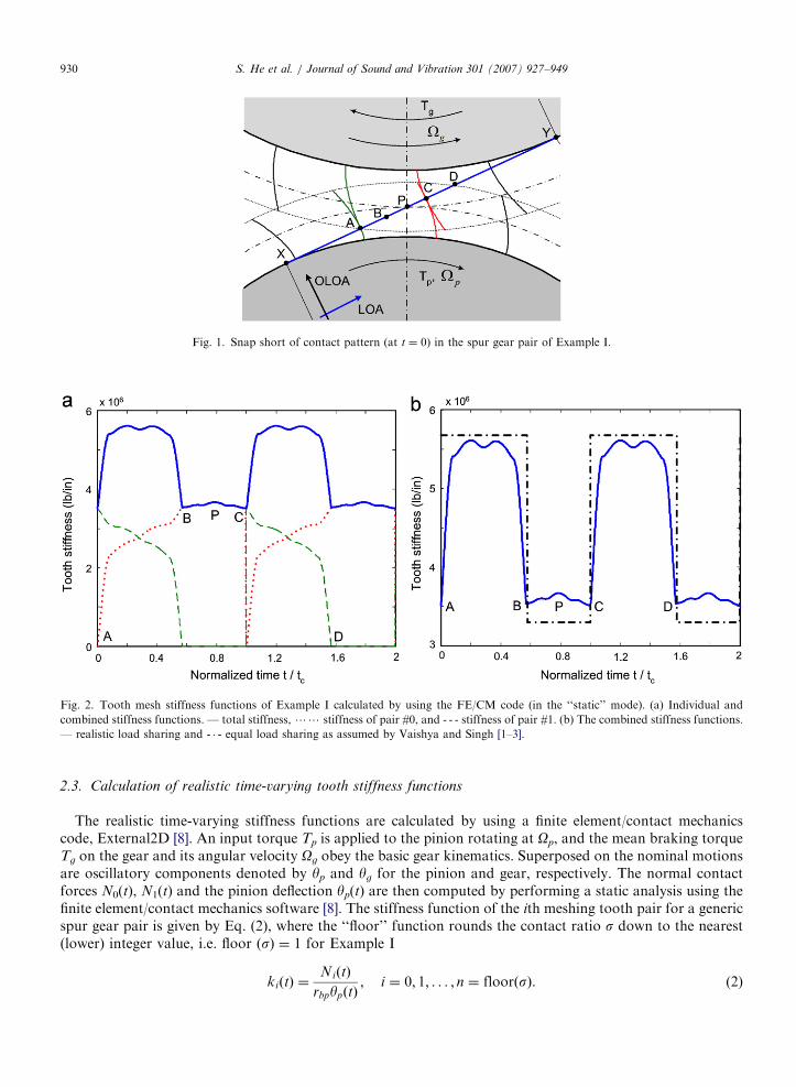
First, transitions in key meshing events within a mesh cycle need to be determined from the undeformedgear geometry for the construction of the stiffness function. Fig. 1 is a snapshot for Example I at the beginning

ARTICLE IN PRESS

Table 1

Parameters of Example I: NASA-ART spur gear pair (non-unity ratio)

Parameter/property Pinion Gear

Number of teeth 25 31

Diametral pitch, in�1 8 8

Pressure angle, deg 25 25

Outside diameter, in 3.372 4.117

Root diameter, in 2.811 3.561

Face width, in 1.250 1.250

Tooth thickness, in 0.196 0.196

Gear mass, lb s2 in�1 6.72E�03 1.04E�02

Polar moment of inertia, lb s2 in 8.48E�03 2.00E�02

Bearing stiffness (LOA and OLOA), lb in�1 20E6

Center distance, in 3.5

Profile contact ratio 1.43

Elastic modulus, psi 30E6

Density, lb s�2 in�4 7.30E�04

Poisson’s ratio 0.3

Table 2

Parameters of Example II-A and II-B: NASA spur gear pair (unity ratio). Gear pair with the perfect involute profile is designated as II-A

case and the one with tip relief is designated as II-B case

Parameter/property Pinion/Gear

Number of teeth 28

Diametral pitch, in�1 8

Pressure angle, deg 20

Outside diameter, in 3.738

Root diameter, in 3.139

Face width, in 0.25

Tooth thickness, in 0.191

Roll angle where the tip modification starts (for II-B), deg 24.5

Straight tip modification (for II-B), in 7E�04

Center distance, in 3.5

Profile contact ratio 1.63

Elastic modulus, psi 30E6

Density, lb s�2 in�4 7.30E�04

Poisson’s ratio 0.3

Range of temperatures, 1F 104, 122, 140, 158, 176

Range of input torques, lb in 500, 600, 700, 800, 900

S. He et al. / Journal of Sound and Vibration 301 (2007) 927–949 929

of the mesh cycle (t ¼ 0). At that time, pair #1 (defined as the tooth pair rolling along line AC) just comes intomesh at point A and pair #0 (defined as the tooth pair rolling along line CD) is in contact at point C, which isthe highest point of single tooth contact (HPSTC). As the gears roll, when pair #1 approaches the lowest pointof single tooth contact (LPSTC) of point B at t ¼ tB, pair #0 leaves contact. At t ¼ tP, pair #1 passes throughthe pitch point P, and the relative sliding velocity of the pinion with respect to the gear is reversed, resulting ina reversal of the friction force. This should provide an impulse excitation to the system. Finally, pair #1 goesthrough point C at t ¼ tc, completing one mesh cycle (tc). These key events are defined below, where Op is thenominal pinion speed, rbp is the base radius of the pinion, length LAC is equal to one base pitch l

tc ¼l

Oprbp

;tb

tc

¼LAB

l;

tp

tc

¼LAP

l. (1a2c)

ARTICLE IN PRESS

Fig. 1. Snap short of contact pattern (at t ¼ 0) in the spur gear pair of Example I.

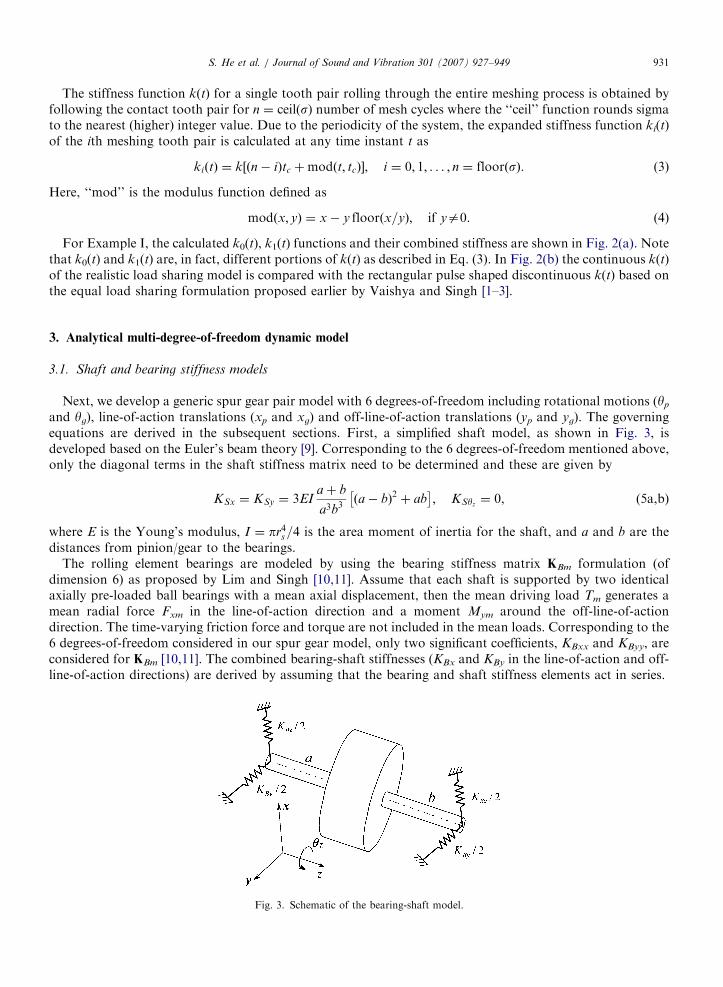
Fig. 2. Tooth mesh stiffness functions of Example I calculated by using the FE/CM code (in the ‘‘static’’ mode). (a) Individual and

combined stiffness functions. — total stiffness, ?? stiffness of pair #0, and - - - stiffness of pair #1. (b) The combined stiffness functions.

— realistic load sharing and - � - equal load sharing as assumed by Vaishya and Singh [1–3].

S. He et al. / Journal of Sound and Vibration 301 (2007) 927–949930

2.3. Calculation of realistic time-varying tooth stiffness functions

The realistic time-varying stiffness functions are calculated by using a finite element/contact mechanicscode, External2D [8]. An input torque Tp is applied to the pinion rotating at Op, and the mean braking torqueTg on the gear and its angular velocity Og obey the basic gear kinematics. Superposed on the nominal motionsare oscillatory components denoted by yp and yg for the pinion and gear, respectively. The normal contactforces N0(t), N1(t) and the pinion deflection yp(t) are then computed by performing a static analysis using thefinite element/contact mechanics software [8]. The stiffness function of the ith meshing tooth pair for a genericspur gear pair is given by Eq. (2), where the ‘‘floor’’ function rounds the contact ratio s down to the nearest(lower) integer value, i.e. floor (s) ¼ 1 for Example I

kiðtÞ ¼NiðtÞ

rbpypðtÞ; i ¼ 0; 1; . . . ; n ¼ floorðsÞ. (2)

ARTICLE IN PRESSS. He et al. / Journal of Sound and Vibration 301 (2007) 927–949 931

The stiffness function k(t) for a single tooth pair rolling through the entire meshing process is obtained byfollowing the contact tooth pair for n ¼ ceil(s) number of mesh cycles where the ‘‘ceil’’ function rounds sigmato the nearest (higher) integer value. Due to the periodicity of the system, the expanded stiffness function ki(t)of the ith meshing tooth pair is calculated at any time instant t as

kiðtÞ ¼ k ðn� iÞtc þmodðt; tcÞ½ �; i ¼ 0; 1; . . . ; n ¼ floorðsÞ. (3)

Here, ‘‘mod’’ is the modulus function defined as

modðx; yÞ ¼ x� y floorðx=yÞ; if ya0. (4)

For Example I, the calculated k0(t), k1(t) functions and their combined stiffness are shown in Fig. 2(a). Notethat k0(t) and k1(t) are, in fact, different portions of k(t) as described in Eq. (3). In Fig. 2(b) the continuous k(t)of the realistic load sharing model is compared with the rectangular pulse shaped discontinuous k(t) based onthe equal load sharing formulation proposed earlier by Vaishya and Singh [1–3].

3. Analytical multi-degree-of-freedom dynamic model

3.1. Shaft and bearing stiffness models

Next, we develop a generic spur gear pair model with 6 degrees-of-freedom including rotational motions (yp

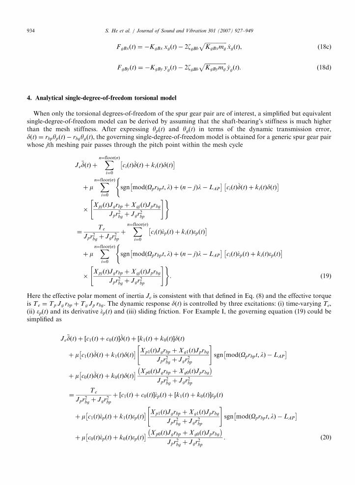
and yg), line-of-action translations (xp and xg) and off-line-of-action translations (yp and yg). The governingequations are derived in the subsequent sections. First, a simplified shaft model, as shown in Fig. 3, isdeveloped based on the Euler’s beam theory [9]. Corresponding to the 6 degrees-of-freedom mentioned above,only the diagonal terms in the shaft stiffness matrix need to be determined and these are given by

KSx ¼ KSy ¼ 3EIaþ b

a3b3ða� bÞ2 þ ab� �

; KSyz¼ 0, (5a,b)

where E is the Young’s modulus, I ¼ pr4s=4 is the area moment of inertia for the shaft, and a and b are thedistances from pinion/gear to the bearings.

The rolling element bearings are modeled by using the bearing stiffness matrix KBm formulation (ofdimension 6) as proposed by Lim and Singh [10,11]. Assume that each shaft is supported by two identicalaxially pre-loaded ball bearings with a mean axial displacement, then the mean driving load Tm generates amean radial force Fxm in the line-of-action direction and a moment Mym around the off-line-of-actiondirection. The time-varying friction force and torque are not included in the mean loads. Corresponding to the6 degrees-of-freedom considered in our spur gear model, only two significant coefficients, KBxx and KByy, areconsidered for KBm [10,11]. The combined bearing-shaft stiffnesses (KBx and KBy in the line-of-action and off-line-of-action directions) are derived by assuming that the bearing and shaft stiffness elements act in series.

Fig. 3. Schematic of the bearing-shaft model.


3.2. Dynamic mesh and friction forces

Fig. 4 depicts the mean torque and the internal reaction forces acting on the pinion for Example I. For thesake of clarity, forces on the gear are not shown, which are equal in magnitude but opposite in direction to thepinion forces. Based on the Coulomb friction law, the magnitude of friction force (Ff) is proportional tothe nominal tooth load (N): jFf j ¼ jmNj, where m is constant. The direction of Ff is determined from thecalculation of the nominal relative sliding velocity, which results in the linear-time-varying systemformulation. Xpi(t) is the moment arm on the pinion for the friction force acting on the ith meshing toothpair and is given by

X piðtÞ ¼ LXA þ ðn� iÞlþmodðOprbpt; lÞ; i ¼ 0; 1; . . . ; n ¼ floorðsÞ. (6)

The corresponding moment arm for the friction force on the gear is

X giðtÞ ¼ LYC þ il�modðOgrbgt; lÞ; i ¼ 0; 1; . . . ; n ¼ floorðsÞ. (7)

Assume, that the mesh (viscous) damping coefficient is time varying and relate it to ki(t) by a time-invariantdamping ratio zm as follows:

ciðtÞ ¼ 2zmi

ffiffiffiffiffiffiffiffiffiffiffiffiffiffiffiffiffikiðtÞ � Je

p; i ¼ 0; 1; . . . ; n ¼ floorðsÞ, (8)

where Je ¼ JpJg=ðJpr2bg þ Jgr2bpÞ.The normal forces acting on the pinion are

NpiðtÞ ¼ NgiðtÞ ¼ kiðtÞ rbp ypðtÞ � rbg ygðtÞ � �pðtÞ þ xpðtÞ � xgðtÞ� �

þ ciðtÞ rbp_ypðtÞ � rbg

_ygðtÞ � _�pðtÞ þ _xpðtÞ � _xgðtÞ� �

; i ¼ 0; 1; . . . ; n ¼ floorðsÞ. ð9Þ

Here eP(t) is the profile error component of the static transmission error (STE), and xp(t) and xg(t) denote thetranslational bearing displacements of pinion and gear, respectively. For a generic spur gear pair whose jthmeshing pair passes through the pitch point within the mesh cycle, the friction forces in the ith meshing pair

Fig. 4. Normal and friction forces of analytical (MDOF) spur gear system model.


are derived as follows:

F pfiðtÞ ¼

mNpiðtÞ; i ¼ 0; 1; . . . ; j � 1;

mNpiðtÞsgn modðOprbpt; lÞ þ ðn� iÞl� LAP

� �; i ¼ j;

�mNpiðtÞ; i ¼ j; j þ 1; . . . ; n ¼ floorðsÞ;

8><>: (10a)

F gfiðtÞ ¼

mNgiðtÞ; i ¼ 0; 1; . . . ; j � 1;

mNgiðtÞsgn modðOgrbgt; lÞ þ ðn� iÞl� LAP

� �; i ¼ j;

�mNgiðtÞ; i ¼ j; j þ 1; . . . ; n ¼ floorðsÞ:

8><>: (10b)

Consequently, the friction forces for Example I of Fig. 4 are given as

Fpf 0ðtÞ ¼ mNp0ðtÞ; Fpf 1ðtÞ ¼ mNp1ðtÞsgn modðOprbpt; lÞ � LAP

� �, (10c,d)

Fgf 0ðtÞ ¼ mNg0ðtÞ; Fgf 1ðtÞ ¼ mNg1ðtÞsgn modðOgrbgt; lÞ � LAP

� �. (10e,f)

3.3. Multi-degree-of-freedom model

The governing equations for the torsional DOFs are

Jp€ypðtÞ ¼ Tp þ

Xn¼floorðsÞ

i¼0

X piðtÞFpfiðtÞ �Xn¼floorðsÞ

i¼0

rbp NpiðtÞ, (11)

Jg€ygðtÞ ¼ �Tg þ

Xn¼floorðsÞ

i¼0

X giðtÞFgfiðtÞ þXn¼floorðsÞ

i¼0

rbg NgiðtÞ. (12)

The governing equations of the translational DOFs in the LOA direction are

mp €xpðtÞ þ 2zpBx

ffiffiffiffiffiffiffiffiffiffiffiffiffiffiffiffiffiKpBx mp

p_xpðtÞ þ KpBxxpðtÞ þ

Xn¼floorðsÞ

i¼0

NpiðtÞ ¼ 0, (13)

mg €xgðtÞ þ 2zgBx

ffiffiffiffiffiffiffiffiffiffiffiffiffiffiffiffiffiKgBx mg

p_xgðtÞ þ KgBxxgðtÞ þ

Xn¼floorðsÞ

i¼0

NgiðtÞ ¼ 0. (14)

Here, KpBx and KgBx are the effective shaft-bearing stiffnesses in the line-of-action direction as discussed inSection 3.1, and zpBx and zgBx are their damping ratios. Similarly, the governing equations of the translationalDOFs in the off-line-of-action direction are

mp €ypðtÞ þ 2zpBy

ffiffiffiffiffiffiffiffiffiffiffiffiffiffiffiffiffiKpBy mp

p_ypðtÞ þ KpByypðtÞ �

Xn¼floorðsÞ

i¼0

FpfiðtÞ ¼ 0, (15)

mg €ygðtÞ þ 2zgBy

ffiffiffiffiffiffiffiffiffiffiffiffiffiffiffiffiffiKgBy mg

p_ygðtÞ þ KgByygðtÞ �

Xn¼floorðsÞ

i¼0

FgfiðtÞ ¼ 0. (16)

The composite DTE, which is the relative dynamic displacement of pinion and gear along the LOA direction,is defined as

dðtÞ ¼ rbpypðtÞ � rbgygðtÞ þ xpðtÞ � xgðtÞ. (17)

Finally, the dynamic bearing forces are given by

F pBxðtÞ ¼ �KpBx xpðtÞ � 2zpBx

ffiffiffiffiffiffiffiffiffiffiffiffiffiffiffiffiKpBxmp

p_xpðtÞ, (18a)

F pByðtÞ ¼ �KpBy ypðtÞ � 2zpBb

ffiffiffiffiffiffiffiffiffiffiffiffiffiffiffiffiKpBymp

p_ypðtÞ, (18b)


F gBxðtÞ ¼ �KgBx xgðtÞ � 2zgBb

ffiffiffiffiffiffiffiffiffiffiffiffiffiffiffiffiKgBxmg

p_xgðtÞ, (18c)

F gByðtÞ ¼ �KgBy ygðtÞ � 2zgBb

ffiffiffiffiffiffiffiffiffiffiffiffiffiffiffiffiKgBymg

p_ygðtÞ. (18d)

4. Analytical single-degree-of-freedom torsional model

When only the torsional degrees-of-freedom of the spur gear pair are of interest, a simplified but equivalentsingle-degree-of-freedom model can be derived by assuming that the shaft-bearing’s stiffness is much higherthan the mesh stiffness. After expressing yp(t) and yg(t) in terms of the dynamic transmission error,dðtÞ ¼ rbpypðtÞ � rbgygðtÞ, the governing single-degree-of-freedom model is obtained for a generic spur gear pairwhose jth meshing pair passes through the pitch point within the mesh cycle

Je€dðtÞ þ

Xn¼floorðsÞ

i¼0

ciðtÞ_dðtÞ þ kiðtÞdðtÞ� �

þ mXn¼floorðsÞ

i¼0

sgn modðOprbpt; lÞ þ ðn� jÞl� LAP

� �ciðtÞ_dðtÞ þ kiðtÞdðtÞ� �(

�X pjðtÞJgrbp þ X gjðtÞJprbg

Jpr2bg þ Jgr2bp

" #)

¼Te

Jpr2bg þ Jgr2bp

þXn¼floorðsÞ

i¼0

ciðtÞ_�pðtÞ þ kiðtÞ�pðtÞ� �

þ mXn¼floorðsÞ

i¼0

sgn modðOprbpt; lÞ þ ðn� jÞl� LAP

� �(ciðtÞ_�pðtÞ þ kiðtÞ�pðtÞ� �

�X pjðtÞJgrbp þ X gjðtÞJprbg

Jpr2bg þ Jgr2bp

" #). ð19Þ

Here the effective polar moment of inertia Je is consistent with that defined in Eq. (8) and the effective torqueis Te ¼ Tp Jg rbp þ Tg Jp rbg. The dynamic response d(t) is controlled by three excitations: (i) time-varying Te,(ii) ep(t) and its derivative _�pðtÞ and (iii) sliding friction. For Example I, the governing equation (19) could besimplified as

Je€dðtÞ þ c1ðtÞ þ c0ðtÞ½ �_dðtÞ þ k1ðtÞ þ k0ðtÞ½ �dðtÞ

þ m c1ðtÞ_dðtÞ þ k1ðtÞdðtÞ� � X p1ðtÞJgrbp þ X g1ðtÞJprbg

Jpr2bg þ Jgr2bp

" #sgn modðOprbpt; lÞ � LAP

� �

þ m c0ðtÞ_dðtÞ þ k0ðtÞdðtÞ� � X p0ðtÞJgrbp þ X g0ðtÞJprbg

� �Jpr2bg þ Jgr2bp

¼Te

Jpr2bg þ Jgr2bp

þ c1ðtÞ þ c0ðtÞ½ �_�pðtÞ þ k1ðtÞ þ k0ðtÞ½ ��pðtÞ

þ m c1ðtÞ_�pðtÞ þ k1ðtÞ�pðtÞ� � X p1ðtÞJgrbp þ X g1ðtÞJprbg

Jpr2bg þ Jgr2bp

" #sgn modðOprbpt; lÞ � LAP

� �

þ m c0ðtÞ_�pðtÞ þ k0ðtÞ�pðtÞ� � X p0ðtÞJgrbp þ X g0ðtÞJprbg

� �Jpr2bg þ Jgr2bp

. ð20Þ


5. Effect of sliding friction in Example I

5.1. Validation of Example I model using the finite element/contact mechanics code

The governing equations of either the single- or multi-degree-of-freedom system models are numericallyintegrated by using a 4th–5th order Runge–Kutta algorithm with a fixed time step. The �pðtÞ and _�pðtÞ

components are neglected, i.e. no manufacturing errors other than specified profile modifications areconsidered. Concurrently, the dynamic responses are independently calculated by running the finite element/contact mechanics code [8] and using the Newmark method. Predicted and computed dynamic transmissionerror, and line-of-action and off-line-of-action forces are in good agreement, as shown in Figs. 5–7. Note thattime domain results include both transient and steady state responses but the frequency domain results onlyinclude the steady state responses. From Fig. 5 it can be seen that the sliding friction introduces additionaldynamic transmission error oscillations when the contact teeth pass through the pitch point. Fig. 6 illustratesthat the sliding friction enhances the dynamic bearing forces in the line-of-action direction, especially at thesecond mesh harmonic. This is because that the moments associated with Fpfi(t) and Fgfi(t) are coupled with themoments of Npi(t) and Ngi(t). Further, the normal loads mainly excite the vibration in the line-of-actiondirection, as illustrated by Eqs. (9), (11) and (13). The scales of the bearing forces shown in Figs. 7(a–b) for them ¼ 0 case are the same as those shown in Figs. 7(c–d) for ease of comparison. The bearing forces predicted by

Fig. 5. Validation of the analytical (MDOF) model by using the FE/CM code (in the ‘‘dynamic’’ mode). Here, results for Example I are

given in terms of d(t) and its spectral contents D(f) with tc ¼ 2.4ms and fm ¼ 416.7Hz. Sub-figures (a–b) are for m ¼ 0 and (c–d) are for

m ¼ 0.2. — Analytical (MDOF) model, ?? FE/CM code (in t domain), and J FE/CM code (in f domain).

ARTICLE IN PRESS


given in terms of FpBx(t) and its spectral contents FpBx(f) with tc ¼ 2.4ms and fm ¼ 416.7Hz. Sub-figures (a–b) are for m ¼ 0 and (c–d) are

for m ¼ 0.2. — Analytical (MDOF) model, ?? FE/CM code (in t domain) and J FE/CM code (in f domain).


the multi-degree-of-freedom model for m ¼ 0 case approach zero (within the numerical error range). This isconsistent with the mathematical description of Eqs. (15) and (16). Larger deviations at this point are observedin Figs. 7(a–b) for the finite element/contact mechanics analysis. As shown in Fig. 7 the off-line-of-actiondynamics are more significantly influenced by the sliding friction than the line-of-action dynamics, which areshown in Fig. 6. In order to accurately predict the higher mesh harmonics, refined time steps (e.g., more than100 increments per mesh cycle) are needed. Consequently, the finite element/contact mechanics analysis tendsto generate an extremely large data file that demands significant computing time and post-processing work.Meanwhile, the lumped model allows for much finer time resolution while being computationally moreefficient (by at least two orders of magnitude when compared with the finite element/contact mechanicscalculations). Hence, the lumped model could be effectively used to conduct parametric design studies.

5.2. Effect of sliding friction

Fig. 8 shows the calculated dynamic transmission error without an friction, which is almost identical to thestatic transmission error at a very low speed (Op ¼ 2.4 rpm). However, the sliding friction changes the shape ofthe dynamic transmission error curve. During the time interval t 2 ½0; tP�, the friction torque on the pinionopposes the normal load torque as shown in Fig. 4, resulting in a higher value of the normal load that isneeded to maintain the static equilibrium. Also, friction increases the peak-to-peak value of the dynamic

ARTICLE IN PRESS


given in terms of FpBy(t) and its spectral contents FpBy(f) with tc ¼ 2.4ms and fm ¼ 416.7Hz. Sub-figures (a–b) are for m ¼ 0 and (c–d) are

for m ¼ 0.2. — Analytical (MDOF) model, ?? FE/CM code (in t domain) and J FE/CM code (in f domain).

Fig. 8. Effect of m on d(t) based on the linear time-varying SDOF model for Example I at Tp ¼ 2000 lb-in. Here, tc ¼ 1 s. — m ¼ 0 and

?? m ¼ 0.1.


transmission error compared with that of the static transmission error. For the remainder of the mesh cyclet 2 ½tP; tc�, friction torque acts in the same direction as the normal load torque. Thus a small value of thenormal load is sufficient to maintain the static equilibrium. Detailed parametric studies show that theamplitude of second mesh harmonic increases with the effect of sliding friction.


5.3. Multi-degree-of-freedom system resonances

For Example I, the nominal bearing stiffness KpBx ¼ KpBy ¼ KgBx ¼ KgBy ¼ 20� 106 lb/in are much higherthan the averaged mesh stiffness km. The couplings between the rotational and translational degrees-of-freedom in the line-of-action direction are examined by using a simplified 3 degree-of-freedom model assuggested by Kahraman and Singh [12]. Note that the dynamic transmission error is defined asd ¼ rbpyxp � rbgyxg, and the undamped equations of motion are

me 0 0

0 mp 0

0 0 mg

264

375

€d

€xp

€xg

8><>:

9>=>;þ

km km �km

km ðkm þ KpBxÞ �km

�km �km ðkm þ KgBxÞ

264

375

d

xp

xg

8><>:

9>=>; ¼

0

0

0

8><>:

9>=>;. (21)

The effective mass is defined as me ¼ JpJg=ðr2gJp þ r2pJgÞ. The eigensolutions of Eq. (21) yield three naturalfrequencies: Two coupled transverse-torsional modes (f1 and f3) and one purely transverse mode (f2);numerical values are: f1 ¼ 5130Hz, f2 ¼ 8473Hz and f3 ¼ 11,780Hz. Predictions from Eq. (21) match wellwith the numerical simulations using the formulations of Section 3 (though these results are not shownhere). A comparative study verifies that one natural frequency of the multi-degree-of-freedom modelshifts away from that of the single-degree-of-freedom model (6716Hz) due to the torsional–translationalcoupling effects. In the off-line-of-action direction, simulation shows that only one resonance is present atf pBy ¼ ð1=2pÞ

ffiffiffiffiffiffiffiffiffiffiffiffiffiffiffiffiffiffiKpBy=mp

p¼ 9748Hz, which is dictated by the bearing-shaft stiffness.

6. Effect of sliding friction in Example II

Next, the proposed model is applied to Example II with the parameters of Table 2. The chief goal is toexamine the effects of tip relief and sliding friction. Further, analogous experiments were conducted onthe NASA Glenn Research Center Gear Noise Rig [13]. Comparisons with measurements will be given inSection 7.

6.1. Empirical coefficient of friction

The coefficient of friction varies as the gears travel through mesh, due to constantly changing lubricationconditions between the contact teeth. An empirical equation for the prediction of the dynamic frictionvariable, m, under mixed lubrication has been suggested by Benedict and Kelley [14] based on a curve-fit offriction measurements on a roller test machine. Rebbechi et al. [15] verified this formulation by measuring thedynamic friction forces on the teeth of a spur gear pair. Their measurements seem to be in good agreementwith the Benedict and Kelley equation except at the meshing positions close to the pitch point. This empiricalequation, then modified to account for the average gear tooth surface roughness (Ravg), is

mðgÞ ¼ 0:0127CRavglog10

3:17� 108XGðgÞW n

noVsðgÞV 2eðgÞ

!; CRavg

¼44:5

44:5� Ravg, (22a,b)

where CRavgis the surface roughness constant, Wn is the normal load per unit length of face width, and u0

is the dynamic viscosity of the lubricant. Here Vs(g) is the sliding velocity, defined as the difference in thetangential velocities of the pinion and gear, and Ve(g) is the entraining velocity, defined as the additionof the tangential velocities, for roll angle g along the line-of-action. Further, Ravg in our case wasmeasured with a profilometer by using a standard method described in Ref. [13]. Lastly, XG(g) is the loadsharing factor as a function of roll angle, and it was assumed based on the ideal profile of smoothmeshing gears. In Fig. 9 m is shown as a function of roll angle calculated by using Eq. (22). Since m wasassumed to be a constant earlier, an averaged value is found by taking an average over the roll angles. The mvalues that were computed at each mean torque and oil temperature for Example II (with Ravg ¼ 0.132 mm)are given in Table 3.

ARTICLE IN PRESS

Fig. 9. The coefficient of friction m as a function of the roll angle for Example II, as predicted by using Benedict & Kelley’s empirical

equation [14]. Here, oil temperature is 104 1F and T ¼ 500 lb-in. P: Pitch point at 20.851.

Table 3

Averaged coefficient of friction m predicted over a range of operating conditions for Example II by using Benedict and Kelly’s empirical

equation [14]

Temperature (1F) Torque (lb-in)

500 600 700 800 900

104 0.032 0.033 0.034 0.035 0.036

122 0.034 0.036 0.037 0.037 0.038

140 0.036 0.037 0.038 0.039 0.040

158 0.038 0.040 0.041 0.041 0.042

176 0.040 0.041 0.042 0.043 0.044


6.2. Effect of tip relief on STE and k(t)

The static transmission error is calculated as a function of mean torque for both the perfect involute gearpair (designated as II-A) and then one with tip relief (designated as II-B) by using the Finite element/contactmechanics code. The amplitudes of the static transmission error spectra at mesh harmonics for both cases areshown in Fig. 10. (In this and following figures, predictions are shown as continuous lines for the sake ofclarity though they are calculated only at discrete torque points). The first two mesh harmonics are mostsignificantly affected by the tip relief and they are minimal at the ‘‘optimal’’ mean torque around 500 lb-in. Forboth II-A and II-B cases, typical k(t) functions of a single meshing tooth over two complete mesh cycles arecalculated by using Eq. (2) for various mean torques, as shown in Fig. 11. Note that k(t) is defined as theeffective stiffness since it incorporates the effects of profile modification such as linear tip relief (II-B). Observethat although the maximum stiffness remains the same, application of the tip relief significantly changes thestiffness profile. For the perfect involute profile (II-A), steep slopes are observed in the vicinities near the singleor two teeth contact regimes, and a smooth transition is observed in between these steep regimes. Also, k(t) isfound to be insensitive to a variation in the mean torque. However, with tip relief, an almost constant slope isfound throughout the transition profile between the single and two teeth contact regimes. Moreover, a smallerprofile contact ratio (around 1.1 at 100 lb-in) is observed for the tip relief case when compared with around 1.6(at all loads) for the perfect involute pair. The realistic k(t) function is then incorporated into the lumpedmulti-degree-of-freedom dynamic model.

ARTICLE IN PRESS

Fig. 10. Mesh harmonics of the static transmission error (STE) calculated by using the FE/CM code (in the ‘‘static’’ mode) for Example II:

(a) gear pair with perfect involute profile (II-A) and (b) gear pair with tip relief (II-B). — n ¼ 1, - - n ¼ 2, and ?? n ¼ 3.

Fig. 11. Tooth stiffness functions of a single mesh tooth pair for Example II: (a) gear pair with perfect involute profile (II-A); (b) gear pair

with tip relief (II-B). — 100 lb-in, ?? 500 lb-in, and - - - 900 lb-in.


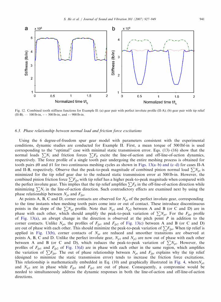
In Fig. 12 the combined k(t) is shown with contributions of both meshing tooth pairs over two mesh cyclesfor Example II. Observe that the profile of case II-A is insensitive to a variation in the mean torque, but theprofile of case II-B has a minimum around 500 lbf-in. Frequency domain analysis reveals that the first twomesh harmonics are most significantly affected by the linear tip modification. Overall, it is evident thatsignificant changes take place in the static transmission error, tooth load distribution and mesh stiffnessfunction because of the profile modification (tip relief), which may be explained by an avoidance of the cornercontact at an ‘‘optimized’’ mean torque.

ARTICLE IN PRESS

Fig. 12. Combined tooth stiffness functions for Example II: (a) gear pair with perfect involute profile (II-A); (b) gear pair with tip relief

(II-B). — 100 lb-in, - � - 500 lb-in, and - - 900 lb-in.


6.3. Phase relationship between normal load and friction force excitations

Using the 6 degree-of-freedom spur gear model with parameters consistent with the experimentalconditions, dynamic studies are conducted for Example II. First, a mean torque of 500 lbf-in is usedcorresponding to the ‘‘optimal’’ case with minimal static transmission error. Eqs. (13)–(16) show that thenormal loads

PNi and friction forces

PFfi excite the line-of-action and off-line-of-action dynamics,

respectively. The force profile of a single tooth pair undergoing the entire meshing process is obtained fortooth pairs #0 and #1 for two continuous meshing cycles as shown in Figs. 13(a–b) and (c–d) for cases II-Aand II-B, respectively. Observe that the peak-to-peak magnitude of combined pinion normal load

PNpi is

minimized for the tip relief gear due to the reduced static transmission error at 500 lb-in. However, thecombined pinion friction force

PFfpi with tip relief has a higher peak-to-peak magnitude when compared with

the perfect involute gear. This implies that the tip relief amplifiesP

Ffi in the off-line-of-action direction whileminimizing

PNi in the line-of-action direction. Such contradictory effects are examined next by using the

phase relationship between Npi and Ffpi.At points A, B, C and D, corner contacts are observed for Npi of the perfect involute gear, corresponding

to the time instants when meshing tooth pairs come into or out of contact. These introduce discontinuouspoints in the slope of the

PNpi profile. Note that Np1 and Np2 between A and B (or C and D) are in

phase with each other, which should amplify the peak-to-peak variation ofP

Npi. For the Ffpi profileof Fig. 13(a), an abrupt change in the direction is observed at the pitch point P in addition to thecorner contacts. Unlike Npi, the profiles of Ffp1 and Ffp2 of Fig. 13(c) between A and B (or C and D)are out of phase with each other. This should minimize the peak-to-peak variation of

PFfpi. When tip relief is

applied in Fig. 13(b), corner contacts of Npi are reduced and smoother transitions are observed atpoints A, B, C and D. Unlike the perfect involute gear, Np1 and Np2 are now out of phase with each otherbetween A and B (or C and D), which reduces the peak-to-peak variation of

PNpi. However, the

profiles of Ffp1 and Ffp2 of Fig. 13(d) are in phase with each other in the same region, which amplifiesthe variation of

PFfpi. The out of phase relationship between Npi and Ffpi explains why the tip relief

(designed to minimize the static transmission error) tends to increase the friction force excitations.This relationship is mathematically embedded in Eq. (10) and graphically illustrated in Fig. 4, whereNp1

and Np2 are in phase while Ffp1 and Ffp2 are out of phase. Consequently, a compromise would beneeded to simultaneously address the dynamic responses in both the line-of-action and off-line-of-actiondirections.

ARTICLE IN PRESS

Fig. 13. Dynamic loads predicted for Example II at 500 lb-in, 4875 RPM and 140 1F with tc ¼ 0.44ms: (a) Normal loads of gear pair with

perfect involute profile (II-A), (b) normal loads of gear par with tip relief (II-B), and (c) friction forces of gear pair with perfect involute

profile (II-A); (d) friction forces of gear pair with tip relief (II-B). — combined, ?? tooth pair #0 and - - tooth pair #1.


6.4. Prediction of the dynamic responses

Dynamic responses including xp(t), yp(t), Fpbx(t), Fpby(t) and the dynamic transmission error d(t) arepredicted by numerically integrating the governing equations. Predictions from both perfect and tip relief


gears are compared to examine the effect of profile modification in the presence of sliding friction. FromFig. 14 it can be seen that the normalized xp(t) at 500 lb-in is much smaller (over 90% reduction) whenthe tip relief is applied. This is because that the STE is the most dominant excitation in the line-of-action

Fig. 14. Dynamic shaft displacements predicted for Example II at 500 lb-in, 4875 RPM and 140 1F with tc ¼ 0.44 ms and fm ¼ 2275Hz: (a)

xp(t), (b) Xp(f), (c) yp(t) and (d) Yp(f). - - - gear pair with perfect involute profile in t domain (II-A), J with perfect involute profile in f

domain (II-A) and — with tip relief (II-B).

Fig. 15. Dynamic transmission error predicted for Example II at 500 lb-in, 4875 RPM and 140 1F with tc ¼ 0.44 ms and fm ¼ 2275Hz: (a)

d(t) and (b) D(f). - - - gear pair with perfect involute profile in t domain (II-A), J with perfect involute profile in f domain (II-A), and —

with tip relief (II-B).


direction and it is minimized at 500 lb-in when the tip relief is applied. An alternative explanation is that thepeak-to-peak variation of

PNpi is minimized with the tip relief as shown in Fig. 13.

In the off-line-of-action direction, more significant oscillations are observed for yp(t) due to increasedP

Ffpi

excitations with tip relief. Despite that the vibratory components ofP

Npi are larger than those ofP

Ffpi, thepredicted yp(t) is actually higher than xp(t). This shows the necessity of including sliding friction when otherexcitations such as the static transmission error are minimized. It is worthwhile to notice that a phasedifference is present in the simulated yp(t) before and after the tip relief is applied. Predicted pinion bearingforces are not shown here since they depict the same features shown in the displacement responses of Fig. 14.The dynamic transmission error predictions, as defined by Eq. (17), with and without the tip relief are shownin Fig. 15. From the similarities between Figs. 14(a–b) and 15(a–b) it is implied that the relative line-of-actiondisplacement plays a dominant role in the dynamic transmission error responses. However, this conclusion issomewhat case specific as the dynamic transmission error results depend on the mesh stiffness, bearingstiffness and gear geometry.

7. Experimental validation of Example II models

Experiments corresponding to Example II-B were conducted at the NASA Glenn Research Center (GearNoise Rig) to validate the multi-degree-of-freedom spur gear pair model and to establish the relative influenceof the friction force excitation on the system. Fig. 16 is a photograph of the inside of the gearbox, where abracket was built to hold two shaft displacement probes one inch away from the center of the gear in the line-of-action and off-line-of-action directions [13]. The probes face a steel collar that was machined to fit aroundthe output shaft with minimal eccentricity. Accelerometers were mounted on the bracket, so the motion of thedisplacement probes could be subtracted from the measurements, if necessary. A thermocouple was installedinside the gearbox to measure the temperature of the oil flinging off the gears as they enter into mesh. Thethermocouple position was chosen to be consistent with Benedict and Kelley’s [14] experiment. A commonshaft speed of 4875 rpm was used in all tests so that the first five harmonics of the gear mesh frequency (2275,4550, 6825, 9100, and 11375Hz) do not excite system resonances. Measurements of shaft displacement in theline-of-action and off-line-of-action directions were collected from the proximity sensors over a range of oilinlet temperatures (104, 122, 140, 158 and 176 1F). At each temperature the torque is varied from 500 to 900 lb-in in steps of 100 lb-in.

Fig. 16. Sensors inside the NASA gearbox (for Example II-B).


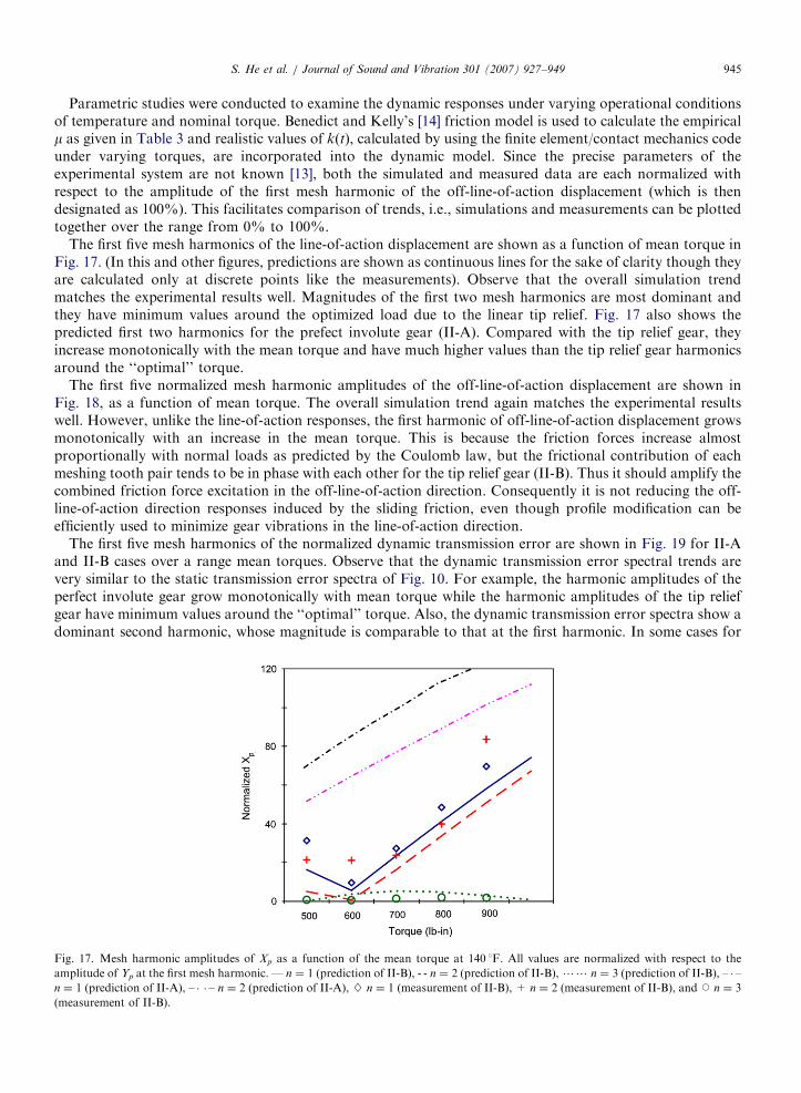
Parametric studies were conducted to examine the dynamic responses under varying operational conditionsof temperature and nominal torque. Benedict and Kelly’s [14] friction model is used to calculate the empiricalm as given in Table 3 and realistic values of k(t), calculated by using the finite element/contact mechanics codeunder varying torques, are incorporated into the dynamic model. Since the precise parameters of theexperimental system are not known [13], both the simulated and measured data are each normalized withrespect to the amplitude of the first mesh harmonic of the off-line-of-action displacement (which is thendesignated as 100%). This facilitates comparison of trends, i.e., simulations and measurements can be plottedtogether over the range from 0% to 100%.

The first five mesh harmonics of the line-of-action displacement are shown as a function of mean torque inFig. 17. (In this and other figures, predictions are shown as continuous lines for the sake of clarity though theyare calculated only at discrete points like the measurements). Observe that the overall simulation trendmatches the experimental results well. Magnitudes of the first two mesh harmonics are most dominant andthey have minimum values around the optimized load due to the linear tip relief. Fig. 17 also shows thepredicted first two harmonics for the prefect involute gear (II-A). Compared with the tip relief gear, theyincrease monotonically with the mean torque and have much higher values than the tip relief gear harmonicsaround the ‘‘optimal’’ torque.

The first five normalized mesh harmonic amplitudes of the off-line-of-action displacement are shown inFig. 18, as a function of mean torque. The overall simulation trend again matches the experimental resultswell. However, unlike the line-of-action responses, the first harmonic of off-line-of-action displacement growsmonotonically with an increase in the mean torque. This is because the friction forces increase almostproportionally with normal loads as predicted by the Coulomb law, but the frictional contribution of eachmeshing tooth pair tends to be in phase with each other for the tip relief gear (II-B). Thus it should amplify thecombined friction force excitation in the off-line-of-action direction. Consequently it is not reducing the off-line-of-action direction responses induced by the sliding friction, even though profile modification can beefficiently used to minimize gear vibrations in the line-of-action direction.

The first five mesh harmonics of the normalized dynamic transmission error are shown in Fig. 19 for II-Aand II-B cases over a range mean torques. Observe that the dynamic transmission error spectral trends arevery similar to the static transmission error spectra of Fig. 10. For example, the harmonic amplitudes of theperfect involute gear grow monotonically with mean torque while the harmonic amplitudes of the tip reliefgear have minimum values around the ‘‘optimal’’ torque. Also, the dynamic transmission error spectra show adominant second harmonic, whose magnitude is comparable to that at the first harmonic. In some cases for

Fig. 17. Mesh harmonic amplitudes of Xp as a function of the mean torque at 140 1F. All values are normalized with respect to the

amplitude of Yp at the first mesh harmonic. — n ¼ 1 (prediction of II-B), - - n ¼ 2 (prediction of II-B),?? n ¼ 3 (prediction of II-B), – � –

n ¼ 1 (prediction of II-A), – � � – n ¼ 2 (prediction of II-A), } n ¼ 1 (measurement of II-B), + n ¼ 2 (measurement of II-B), and J n ¼ 3

(measurement of II-B).

ARTICLE IN PRESS

Fig. 19. Predicted dynamic transmission errors (DTE) for Example II over a range of torque at 140 1F: (a) gear pair with perfect involute

profile (II-A) and (b) with tip relief (II-B). All values are normalized with respect to the amplitude of d (II-A) at the first mesh harmonic

with 100 lb-in. — n ¼ 1 (II-B), - - n ¼ 2 (II-B), and ?? n ¼ 3 (II-B).

Fig. 18. Mesh harmonic amplitudes of yp as a function of the mean torque at 140 1F for Example II-B. All values are normalized with

respect to the amplitude of yp at the first mesh harmonic. — n ¼ 1 (prediction of II-B), - - n ¼ 2 (prediction of II-B),?? n ¼ 3 (prediction

of II-B), } n ¼ 1 (measurement of II-B), + n ¼ 2 (measurement of II-B), and J n ¼ 3 (measurement of II-B).


the tip relief gear the second harmonic becomes the most dominant component especially when the meantorque is lower than 350 lb-in.

Finally, the first five mesh harmonics of the normalized line-of-action displacement are shown in Fig. 20 as afunction of the operational temperature. The changes in temperature are converted into a variation in friction(m) by using the data in Table 3. Compared with the off-line-of-action motions, both predictions andmeasurements in the line-of-action direction give almost identical results at all temperatures. Fig. 21 shows thefirst five normalized mesh harmonic amplitudes of the off-line-of-action displacement as a function oftemperature. The first harmonic varies quite significantly even though the changes in m are relativelysmall. Consequently, the off-line-of-action dynamics tends to be much more sensitive than the onlineaction dynamics to a variation in m. Measured data in Fig. 21 show some variations due to the experimentalerrors [13].

ARTICLE IN PRESS

Fig. 20. Mesh harmonic amplitudes of xp as a function of temperature at 500 lb-in for Example II-B. All values are normalized with



Fig. 21. Mesh harmonic amplitudes of yp as a function of temperature at 500 lb-in for Example II-B. All values are normalized with




8. Conclusion

The chief contribution of this paper is the development of a new multi-degree of freedom, linear time-varying model. This formulation overcomes the deficiency of Vaishya and Singh’s work [1–3] by employingrealistic tooth stiffness functions and the sliding friction over a range of operational conditions. Refinementsinclude: (1) an accurate representation of tooth contact and spatial variation in tooth mesh stiffness based on afinite element/contact mechanics code in the ‘‘static’’ mode; (2) a Coulomb friction model for sliding resistancewith an empirical coefficient of friction that is a function of operation conditions; (3) a better representation of


the coupling between the line-of-action and off-line-of-action directions including torsional and translationaldegrees of freedom. Numerical solutions of the multi-degree-of-freedom model yield the dynamic transmissionerror and vibratory motions in the line-of-action and off-line-of-action directions. The new model has beensuccessfully validated first by using the finite element/contact mechanics code while running in the ‘‘dynamic’’mode and then by analogous experiments. Since the lumped model is more computationally efficient than thefinite element/contact mechanics analysis, it could be quickly used to study the effects of varying a largenumber of parameters.

One of the main effects of sliding friction is the enhancement of the dynamic transmission error magnitudeat the second gear mesh harmonic. A key question of whether the sliding friction is indeed the source of theoff-line-of-action motions and forces is then answered by our model. The bearing forces in the line-of-actiondirection are influenced by the normal tooth loads, but the sliding frictional forces primarily excite the off-line-of-action motions. Finally, the effect of the profile modification on the dynamic transmission error has beenanalytically examined under the influence of frictional effects. For instance, the tip relief introduces anamplification in the off-line-of-action motions and forces due to an out of phase relationship between thenormal load and friction forces. This knowledge should be of significant utility to designers. Future modelingwork should include an examination of the effects of other profile modifications to determine the conditionsfor minimal dynamic responses when both static transmission error and friction excitations are simultaneouslypresent. Also, the model could be further refined by incorporating alternative friction formulations.

Acknowledgments

This article is based upon a three-year study that was supported by the US Army Research Laboratory andthe US Army Research Office under contract/grant number DAAD19-02-1-0334. This support and theencouragement by Dr. G. L. Anderson (project monitor) are gratefully acknowledged. Dr. S. Vijayakar(Advanced Numerical Solutions, Inc.) is thanked for providing access to the External2D gear analysissoftware. We acknowledge the experimental work conducted by V. Asnani and the calculation of empiricalcoefficients of friction performed by A. Holob, both from the Acoustics and Dynamics Laboratory at TheOhio State University; these studies are reported in [15]. Dr. T. Lim from the University of Cincinnati isthanked for providing the Rebm3.0 software for calculation of the bearing stiffness. Finally, we thank theMechanical Components Branch of the NASA Glenn Research Center for providing us with the experimentalfacilities.

References

[1] M. Vaishya, R. Singh, Analysis of periodically varying gear mesh systems with Coulomb friction using Floquet theory, Journal of

Sound and Vibration 243 (3) (2001) 525–545.

[2] M. Vaishya, R. Singh, Sliding friction-induced non-linearity and parametric effects in gear dynamics, Journal of Sound and Vibration

248 (4) (2001) 671–694.

[3] M. Vaishya, R. Singh, Strategies for modeling friction in gear dynamics, ASME Journal of Mechanical Design 125 (2003) 383–393.

[4] D.R. Houser, M. Vaishya, J.D. Sorenson, Vibro-acoustic effects of friction in gears: an experimental investigation, SAE (2001) paper

No. 2001-01-1516.

[5] P. Velex, V. Cahouet, Experimental and numerical investigations on the influence of tooth friction in spur and helical gear dynamics,

ASME Journal of Mechanical Design 122 (4) (2000) 515–522.

[6] P. Velex, P. Sainsot, An analytical study of tooth friction excitations in spur and helical hears, Mechanism and Machine Theory 37

(2002) 641–658.

[7] O. Lundvall, N. Stromberg, A. Klarbring, A flexible multi-body approach for frictional contact in spur gears, Journal of Sound and

Vibration 278 (3) (2004) 479–499.

[8] External2D (CALYX software), A contact mechanics/finite element (CM/FE) tool for spur gear design, ANSOL Inc., Hilliard, OH.

[9] H. Vinayak, R. Singh, C. Padmanabhan, Linear dynamic analysis of multi-mesh transmissions containing external, rigid gears,

Journal of Sound and Vibration 185 (1) (1995) 1–32.

[10] T.C. Lim, R. Singh, Vibration transmission through rolling element bearings. Part I: bearing stiffness formulation, Journal of Sound

and Vibration 139 (2) (1990) 179–199.

[11] T.C. Lim, R. Singh, Vibration transmission through rolling element bearings. Part II: system studies, Journal of Sound and Vibration

139 (2) (1991) 201–225.


[12] A. Kahraman, R. Singh, Error associated with a reduced order linear model of spur gear pair, Journal of Sound and Vibration 149 (3)

(1991) 495–498.

[13] R. Singh, Dynamic analysis of sliding friction in rotorcraft geared systems, technical report submitted to the Army Research Office,

grant number DAAD19-02-1-0334, 2005.

[14] G.H. Benedict, B.W. Kelley, Instantaneous coefficients of gear tooth friction, Transactions of the American Society of Lubrication

Engineers 4 (1961) 59–70.

[15] B. Rebbechi, F.B. Oswald, D.P. Townsend, measurement of gear tooth dynamic friction, ASME Power Transmission and Gearing

Conference proceedings DE-Vol. 88, 1996, pp. 355–363.

Date post:	06-Sep-2018
Category:	Documents
Upload:	buinga
View:	216 times
Download:	0 times

Effect of sliding friction on the dynamics of spur gear ... et al... · The chief objective of this...

Documents