University of Hohenheim Faculty of Agricultural Sciences Institute for Plant Production and Agroecology in the Tropics and Subtropics Crop Waterstress Management in the Tropics and Subtropics (380c) Effects of Vegetation Type and Species Composition on Carbon Stocks in semi-arid Ethiopian Savannahs Beatrice Breuer M. Sc. Thesis This Master Thesis was financially supported by Dr. Hermann Eiselen Stipendienförderung – Fiat Panis Hohenheim, October 2012
Transcript
University of Hohenheim
Faculty of Agricultural Sciences
Institute for Plant Production and Agroecology in the Tropics and Subtropics
Crop Waterstress Management in the Tropics and Subtropics (380c)
Effects of Vegetation Type and Species
Composition on Carbon Stocks in semi-arid
Ethiopian Savannahs
Beatrice Breuer
M. Sc. Thesis
This Master Thesis was financially supported by Dr. Hermann Eiselen
Stipendienförderung – Fiat Panis
Hohenheim, October 2012
Main Supervisor: Prof Dr. Folkard Asch
Co Supervisor: Prof. Dr. Karl Stahr
I
Declaration
I, Beatrice Breuer, born on the 16th of September 1985, Matriculation number: 394949,
hereby declare on my honor, that this Master Thesis entitled
“EFFECTS OF VEGETATION TYPE AND SPECIES COMPOSITION ON CARBON
STOCKS IN SEMI-ARID ETHIOPIAN SAVANNAHS”,
has been independently prepared, solely with the support of the listed literature references,
and that no information has been presented that has not been officially acknowledged.
I declare, here within, that I have transferred the final digital text document (in the format doc,
docx, odt, pdf, or rtf) to my mentoring supervisor and that the content and wording is entirely
my own work. I am aware that the digital version of my document can and/or will be checked
for plagiarism with the help of an analyses software program.
Supervisor: Prof. Dr. Folkard Asch
Prof. Dr. Karl Stahr
Thesis topic: Effects of vegetation type and species composition on carbon stocks in semi-
arid Ethiopian savannahs
Semester: 6
City, Date, Signature
II
Acknowledgement
Many thanks go to Prof. Dr. Folkard Asch for the great opportunity to work in this project and
his supervising and support during the field work and the research period. I also want to thank
Dipl.-Biol. Sabine Stürz for the support during some statistical problems and for the
encouragement. Then I want to thank Prof. Dr. Karl Stahr, for being my co-supervisor.
For the financial support, I would like to thank the Hermann Eiselen Foundation – Fiat Panis.
Thanks to the people, in the laboratory for their great advice and their patience during our
work: Holger Fischer, Natalia Egana, Elke and Beate.
Furthermore, I want to thank Juan Carlos Laso Bayas and Jens Möhring for introducing me in
the world of statistics.
I would like to thank all the people in Ethiopia, who made our stay very comfortable: Dr.
Jürgen Greiling, Alem Greiling, Hasan Yusuf, Addis Shiferaw, Fewen, the “Dabo-Woman”,
and our driver Tamerate, who was always driving us safely, even without breaks.
When talking about Ethiopia, I will never forget our time together – we all had our ups and
downs, but in the end, we worked out very well and no matter what, we always had something
to laugh. I will never miss this great experience with you: Sarah Glatzle, Lena Rathjen and
Jan Pfister.
Special thanks go to my family, especially my parents, who always supported me and my
decisions during my studies and my life. I already had the opportunity to discover so many
nice places in the world, always knowing to have your love in my “backpack”.
I also want to thank Christoph Eisenbeiss – “even if you are at the other side of the world, I
knew, I had you on my side and we always found our way, where the roads were crossing. I
love you.”
Finally, I want to thank my beloved friends, especially Sarah, Sarah (the little one ) and
Nadja for being such an important part in my life – “YOU ARE THE BEST, AND YOU
KNOW IT!!”
III
Abstract
CO2 is one of the most important GHGs in the atmosphere. Its concentration is steadily
increasing, causing severe climate change effects. These changes are of enormous importance
for the people living in the semi-arid savannahs of the Borana region in southern Ethiopia.
Having negative impacts on the pastoral production systems that play an important role in this
area, the dependency on traditional systems might be no longer sufficient to sustain food
security. The establishment of a system of payment for environmental services (PES) could be
a feasible opportunity for alternative income generation. PES systems are based on the
process of carbon sequestration, i.e. storing the atmospheric carbon in the terrestrial
biosphere. In this context, grasslands and savannah ecosystems are increasingly the focus of
attention, as they hold a great potential, due to their large global extension.
The aim of this pilot study was to gain information on the current amount of carbon stored in
the aboveground biomass and in the soil in this area, and to evaluate the impact of vegetation
type and species composition on the belowground carbon stocks.
In a 10 km² study area 4 dominant vegetation types were characterized (grassland, bushland,
tree savannah and bush-tree savannah). 20 30x30 m plots were installed, representing 5 plots
per vegetation type. In every plot, soil samples were taken in 4 depths to determine SOM,
SOC, pH and CaCO3 content. The SOC concentration was measured using the Loss-on-
ignition method. Soil bulk density was measured in 2 depths (0-10, 10-30) with 5 repetitions
each in every plot. Species were identified for the analysis of species composition. Biomass of
trees and bushes was estimated using allometric equations. Biomass of understorey vegetation
was destructively measured. A one-way ANOVA and a cluster analysis were carried out for
the statistical analysis. The vegetation type had a great influence on the accumulation of
aboveground biomass and aboveground carbon stocks, being highest in tree savannahs (51.9 ±
16.1 t ha-1 and 25.9 ± 8.1 t C ha-1), and lowest in grasslands (0.8 ± 0.4 t ha-1 and 0.4 ± 0.2 t C
ha-1). Soil organic carbon stocks were generally high in this area (326.4 ± 28.6 t C ha-1 to
394.9 ± 28.6 t C ha-1) and showed no significant differences between the vegetation types.
Species composition changed to more annuals and herbaceous species with increasing woody
vegetation and cluster analysis showed that the distribution of vegetation types was partially
dependent on the soil type. These results provide initial data to assess the carbon sequestration
potential of the semi-arid savannahs of the Borana region in Ethiopia.
Picture 6 Increased herbaceous production under Acacia tree canopy ................................... 61
Picture 7 Grassland plots on clayey soils before (a) and after (b) the rainy season ................ 62
List of Abbreviations
X
List of Abbreviations
°C degree Celsius
AGB aboveground biomass
AGCS aboveground carbon stocks
B bushland
BD bulk density
BT bush-tree savannah
C carbon
CaCO3 Calcium carbonate
CDM Clean Development Mechanisms
cm centimeter
CO2 carbon dioxide
G grassland
GHG Greenhouse gases
Gt giga ton
ha hectare
kg kilogram
km² square kilometer
m meter
m² square meter
mm millimeter
N nitrogen
PES Payment for environmental services
Pg picogram
ppmv parts per million by volume
SOC soil organic carbon
SOCS soil organic carbon stocks
SOM soil organic matter
t ton
T tree savannah
VT vegetation type
Background
1
1 BACKGROUND This Master-Thesis has been part of the project “Livelihood diversifying potential of livestock
based carbon sequestration options in pastoral and agro pastoral systems in Africa”,
conducted by ILRI (International Livestock Research Institute). One major focus of the
project is the estimation of the carbon sequestration potential of rangelands and the
assessment of how land-use management decisions can avoid or reduce carbon emissions to
the atmosphere. This thesis will provide data about the potential of various vegetation units to
sequester carbon by determining the above and belowground biomass and carbon stocks,
respectively.
Grassland ecosystems, with tropical and subtropical savannahs and woodlands, comprise the
largest terrestrial biome (Hudak et al. 2003). They include rangelands, shrub lands, pasture
land and croplands sown with pasture and fodder crops and cover 3.5 billion ha or26 % of the
world land area (Ramankutty et al. 2008; Conant 2010). A considerable amount (20%) of the
world’s soil organic carbon is stored in grasslands. Globally, about 343 billion tons of C are
estimated to be accumulated in grassland areas (Conant 2010). Anderson (1991) estimated the
soil carbon stocks of the African continent at 30% of the world’s total.
People are dependent on grasslands to a large extend for food and forage production. The
conversion of native grasslands to cultivated croplands has been observed for centuries.
Further, grasslands are the base for milk and beef production and about 1 billion of the
world’s poorest people rely strongly on livestock (Steinfeld et al. 2006).
In the Borana region of southern Ethiopia, livestock production is the main source of income
generation and food security. However, due to increasing climatic changes, like extreme
weather events and the competition with other land uses, this dependency might no longer be
sufficient to sustain food security and alternative possibilities for income generation need to
be considered.
Carbon sequestration would be a feasible opportunity for these poor, vulnerable and
marginalized pastoral and agro-pastoral communities to diversify their income. One
possibility could be the payment for environmental services (PES). These are based on the
carbon sequestration potential and the decline in carbon emissions which are related to
livestock and rangeland management practices (Reid et al. 2004). Moreover, industrialized
countries may invest in GHG emission mitigation projects in developing countries.
Developing countries can then sell the sequestered C in agro-forestry systems to industrialized
countries, which is an attractive economic chance for subsistence farmers (IPCC 2000;
Takimoto et al. 2008).
Introduction
2
2 INTRODUCTION
CO2 is one of the most important Greenhouse gases (GHGs). Over the last centuries its
concentration in the atmosphere has noticeably increased, namely from 280 ppmv in 1750 to
380 ppmv in 2005 (Lal 2004b; Lal 2008a), and it is predicted that the concentration of CO2
and other GHGs will rise even more. The current rate of increment of CO2 is 1.7 ppmv yr-1
(IPCC 2007).
This leads to changes, especially in the global climate. These changes include rising
temperatures and more extreme events of erratic rainfalls. This goes along with higher
incidences of drought and floods (USDA NRCS 2000). In dry areas, with low soil cover
during dry periods, soil respiration is enhanced and the vulnerability to soil erosion and run-
off due to erratic rainfall increases. As a consequence, the soil organic carbon (SOC) pool will
decrease as well as the structural stability of the soil. Thereby, major soil cycles (water,
carbon and nitrogen) are disrupted (Lal 2004b).
These changes are of enormous importance especially for people living on the Borana
Plateau, which belongs to the semi-arid rangelands of Southern Ethiopia (Coppock 1994). It
has negative impacts on the pastoral production systems which play an important role in this
area. In combination with an increasing population pressure, and therefore a challenge to
compete with other land uses, the dependency on traditional pastoral and agro-pastoral
livelihoods is no longer sufficient to sustain food security and the most basic standard of
living.
Hence, a solution has to be found to “remove” carbon (C) from the atmosphere. It has been
suggested, that storing the atmospheric C in the biosphere of the terrestrial system could be
one opportunity to balance the GHG emissions (Albrecht and Kandji 2003).
In general, agricultural lands may have a great potential in terms of C sinks, because they are
able to absorb huge quantities of C. Soils contain twice as much C as the atmosphere and
approximately three-quarters of the total terrestrial organic carbon pool (Prentice et al. 2001).
As reported in the literature, the soil comprises 1115 to 2200 Pg of C (Batjes 1992; Eswaran
et al. 1993; Sombroek et al. 1993). Especially, the combination of trees and crops and/or
animals may store high amounts of C, particularly if they are managed in an equitable way
(Albrecht and Kandji 2003).
Agroforestry systems are already widely recognized as a strategy for soil C sequestration
(Albrecht and Kandji 2003; Takimoto et al. 2008; Nair et al. 2009), especially since forestry
Introduction
3
is a crucial, existing element of the Clean Development Mechanisms (CDM) of the Kyoto
Protocol (FAO 2010).
Nowadays, the role of grasslands and savannah ecosystems and their potential to sequester C
is coming more and more into focus, due to the large global extend of these environments
(Conant et al. 2001; Reid et al. 2004; Witt et al. 2011).
Savannahs cover approximately 20% of the global land cover and even 50% of the African
continent (Ajtay et al. 1979). They are defined by the coexistence of woody (including trees)
and herbaceous or grassy vegetation. Further, they can be classified more in detail by their
relative amounts of these plant functional types (PFTs) (Williams and Albertson 2004).
In grasslands, C is accumulated in two different pools. In the soil, C is stored in dead and
living biomass and aboveground in living biomass and litter. Living aboveground biomass
consists of annual and perennial grasses and woody vegetation like shrubs, bushes and trees.
After Ordóñez et al. (2008), these C pools range from 0.15 t C ha-1 to 33 t C ha-1 in tropical
grasslands. Soil organic carbon (SOC) includes living roots, soil microbial biomass and dead
organic residues. Estimates for tropical grasslands range from 38 to 148 t C ha-1 in the topsoil
(0-30 cm) (Steinbeiss et al. 2007; Ordóñez et al. 2008).
The quantity of litter is very variable and depends strongly on the species composition
(herbaceous or woody vegetation), land use and management factors like burning or
fertilization (Ammann et al. 2007; Shimoda and Takahashi 2009; Sanaullah et al. 2010).
Carbon dynamics (sinks and sources) in grasslands are very complex and depend on a range
of biotic and abiotic factors, including climatic, environmental and management factors as
well as the species composition and their diversity. Chapin et al. (1997) highlighted the
relationship between soil C storage and biodiversity. It is expected, that increasing
biodiversity leads to the protection of the resilience and productivity of grasslands. In
addition, ecosystem service provision is improved on the local scale (Hooper et al. 2005) and
higher biodiversity leads to increased primary productivity (Hector et al. 1999).
However, it is still not so much known about the interconnection between different vegetation
types and C stocks. The main question of this study is, whether the aboveground biomass or
vegetation (formation) type can be used as an indicator to estimate belowground C stocks.
Objectives & Hypothesis
4
3 OBJECTIVES & HYPOTHESIS
3.1 Objectives
The vast grazing areas of the Borana Plateau hold a great potential for carbon sequestration
and thereby reducing the CO2 emissions from the atmosphere. In addition, to protect this area
from further degradation, PES would be a practicable alternative for people living in the
Borana Plateau, who heavily and almost uniquely rely on the production of livestock, to
diversify their income.
This pilot study evaluates the current state of the C-stocks (above- and belowground) of the
Borana Plateau. It gives information about how much carbon is actually stored in the soils and
the vegetation, as this knowledge is crucial for predictions of the potential for carbon
sequestration.
SOC measurements in the field are very accurate and provide site-specific information.
However, they are labor intensive, costly and time consuming. Therefore, this study links
specific vegetation types or vegetation patterns to the organic carbon content stored in the
soil. Through upscaling, this would be a feasible and low cost possibility to predict the carbon
state of larger areas.
Specific objectives of this study were to:
• Identify prominent vegetation types of the area
• Specify these vegetation types in terms of structure and species composition
• Destructively measure biomass of understorey vegetation
• Determine biomass and carbon content of aboveground vegetation with the help of
allometric equations
• Measure organic carbon content of the soil underneath every identified vegetation type
• Link the soil organic carbon content to the respective vegetation type
Objectives & Hypothesis
5
3.2 Hypothesis
Carbon sequestration in agricultural soils and vegetation is meant to be a feasible opportunity
to reduce GHG emissions, and thus to control to a certain extent the ongoing climate change
effects. Tropical and subtropical grassland ecosystems play a major role in this context, due to
their immense expands over the whole world. Savannahs are defined by the coexistence of
woody (trees, bushes/shrubs) and herbaceous vegetation which can occur in different
amounts. As a result of litter composition, carbon inputs, fluxes and storage ability depend on
vegetation.
In this context following hypothesis were tested:
• The aboveground biomass and carbon stored in the vegetation types [t ha-1] will
increase with increasing system diversity and in the order:
Grassland < Bush land < Tree savannah < Bush Tree savannah
• Changes in the main vegetation of aboveground biomass lead to changes in litter
composition, which results in differences in the belowground carbon stocks.
According to the aboveground biomass it is assumed, the higher the systems diversity,
and the higher the aboveground biomass the higher the belowground carbon stocks in
the order: Grassland < Bush land < Tree savannah < Bush Tree savannah
• In terms of carbon distribution with depth, changes in vegetation life form leads to
differences in the main rooting depth and root distribution. In addition, the share of
root biomass in deeper soil layers will be higher in vegetation types with woody
vegetation than without. This contributes to higher carbon inputs and the belowground
carbon stocks will be different among the vegetation types.
• The vegetation types are a result of different vegetation formations. Trees and bushes
deliver additional or unique habitats for specific plant species. In terms of species
diversity and species composition, there will be differences between the vegetation
types. Further, species composition (e.g. the presence of N-fixing legumes) changes
the amount of carbon that can be stored in soils. Therefore, the differences in species
composition result in differences in carbon stocks.
State of the Art
6
4 STATE OF THE ART
4.1 The global Carbon cycle
Carbon (C) is crucial for all life on Earth. The dry weight of most living organisms consist
about half of carbon.
The global carbon cycle is divided into five major C pools; the Atmosphere, Biosphere,
Pedosphere, Hydrosphere and Lithosphere (Figure 1). They are all interconnected by
pathways of exchange (Schlesinger 1997). The process of the C cycling is complex, as C
occurs in different chemical forms in the different pools and various complex processes play a
major role in the fluxes between the pools. In addition, also changes in climate can influence
the atmospheric concentration of CO2 (Lal 2001b).
Figure 1 The global carbon cycle. Red arrows are net fluxes of Carbon in Pg. (ozcoasts.gov.au/glossary/images/ carbon_cyclefig1.jpg)
The largest C pool is the oceanic pool (Hydrosphere), which is estimated at 38,000 Pg and
increasing at the rate of 2.3 Pg C yr-1. The geological C pool (Lithosphere) is estimated at
4130 Pg and mainly consists of fossil fuels, where coal is the main part (85%). The
combustion of fossil fuels plays a major role in releasing CO2 to the atmosphere and thereby
the geological C pool is depleted. The third largest pool is the pedologic pool with around
2500 Pg estimated to 1 m depth. The atmospheric pool consist of around 760 Pg of C, with
CO2 being the most important form. Finally, the biotic pool is the smallest one, where
State of the Art
7
approximately 560 Pg of C is stored. The combination of the pedologic and the biotic pool is
defined as the terrestrial C pool (Lal 2008a).
The cycling of C through the terrestrial
biosphere occurs at varying time scales
(Prentice et al. 2001). One of the most
important fluxes of C is the flux between
the atmosphere and the land vegetation
(Schlesinger 1997; Lal et al. 1998), as it is
the fastest one. The uptake of C by the
vegetation follows a diurnal and seasonal
cycle what is called the “Keeling curve”
(Figure 2). During daytime in the growth
period, vegetation removes CO2 through
photosynthesis from the atmosphere, which
is then stored in organic matter. Depending on various biotic and abiotic factors, CO2 is
returned via plant, soil and microbial respiration. (Falkowski et al. 2000). However, when
conditions are too cold or too dry, these processes are interrupted (Riebeek and Simmon
2011). The gross primary production of the vegetation is about 120Pg C yr-1. This is balanced
by vegetation respiration (60Pg C yr-1) and the decomposition of soil organic matter (SOM)
(60Pg C yr-1) (Lal 2008b). On a global basis, forests form the primary terrestrial C storage
(Falkowski et al. 2000), and have a huge impact on the global C budget. As a result of land
use change, e.g. deforestation, C stored in the living biomass and in the soil is released,
causing an increase in atmospheric CO2. Conversely, in case of reforestation of formerly
agricultural land, C is stored in the newly created biomass and atmospheric CO2
concentrations will decrease (Riebeek and Simmon 2011).
In contrast, fossil fuel reserves and sedimentary rock deposits (like limestone, dolomite and
chalk) in the lithosphere form the relatively immobile stock and are part of the slow C pool
(IPCC 2001). Fluxes in the fast C cycle take place in a lifespan, whereas C in the slow cycle
can resist up to thousands of years.
Therefore, the pedosphere plays a central role in the global C cycle, with a C pool three times
the atmospheric pool and almost four times the biotic pool (Lal 2001a) (Figure 1). A slight
increase or decrease in the net flux of CO2 from the pedosphere would have a significant
impact on the global C budget (Amundson 2001). For instance, a change of 1 Pg of the soil C
pool leads to CO2 changes of 0.47 ppm in the atmosphere (Lal 2001b).
Figure 2 Fluctuations of the atmospheric CO2 concentration (Graph by Robert Simmon, based on data from the NOAA Climate Monitoring & Diagnostics Laboratory)
State of the Art
8
Current CO2 concentration in the atmosphere was estimated to be 391 ppmv or 0.0391%
(Tans 2012) and is increasing at the rate of 0.5 % yr-1.
The role of Africa in the global C cycle becomes increasingly interesting. However, the
knowledge about its potential is still notably limited. Current studies mainly concentrate on
the emissions of C due to land use change and fires (Williams et al. 2007a; Ciais et al. 2011),
as these are the most important contributors in Africa. On the other hand, the C sequestration
potential of grasslands, savannahs and agroforestry systems, which are covering vast areas of
Africa, is meant to be outstanding (Williams et al. 2007a). Therefore, it has yet to be
identified, whether Africa is a net sink or source of atmospheric C.
4.2 Carbon pools in the soil
The pedologic C pool can be mainly subdivided into two; the soil organic carbon (SOC) and
the soil inorganic carbon (SIC). Globally, the pedosphere stores about 2500 Pg C of which
1550 Pg is accumulated in the SOC pool and 950 Pg in the SIC pool (Lal 2008a).
The SIC pool consists of elemental C and carbonate minerals like calcite, dolomite and
gypsum, and encompasses primary and secondary carbonates. The primary carbonates result
through the process of weathering of parent material. Secondary carbonates are formed
through the decomposition/resolution of carbonate bearing minerals and the re-precipitation
of weathering products. In addition they can be built through the chemical reaction of
atmospheric CO2 with Ca2+ and Mg2+ or other salts in soils, which are entering the local
ecosystem e.g. in form of calcareous dust, irrigation water, fertilizer or manure. The process
of secondary carbonate formation and leaching of carbonate and bicarbonate lead to the
sequestration of inorganic C in soils, and are of major importance i.e. in arid and semiarid
regions (Lal 2001b; Lal 2008a).
The SOC pool is composed of highly active humus and comparatively immobile charcoal C.
The soil organic matter (SOM) content of soils is the major determinant of SOC, as it is the
sum of all organic C-including substances in soils. It is assumed, that SOC has a share of
approximately 58% in SOM (Batjes 1996). SOM consists of a mixture of plant and animal
residues in different phases of decomposition, of substances which are synthesized through
microbial activity and/or chemical breakdown of products. Further it consists of living
biomass other than plants, like micro-organisms and small animals (Schnitzer 1991;
Amundson 2001). In general, SOM is subdivided into humic and non-humic substances. The
latter are substances which have still recognizable chemical characteristics like carbohydrates,
proteins, peptides, amino acids, fatty acids and waxes. These compounds are degraded in soils
State of the Art
9
relatively easily and their life span is short. Humic substances are materials which are
amorphous, dark-colored, hydrophilic or aromatic. They build up the major part of SOM and
are less susceptible to chemical and biological degradation (Schnitzer 1991).
The whole SOC pool is divided into three different parts which are distinguished according to
their time of residence (Parton et al. 1987). The first one is the active or labile pool. It
comprises mainly young SOM like fresh plant material and root exudates that are relatively
easily degradable. Thus the labile pool has a rapid turnover, which leads to a resting time
usually not more than one year. Since it is very sensitive to land management and
environmental conditions, it may significantly influence the short-term C and N-cycling in
terrestrial ecosystems (Schlesinger et al. 1990). The second one is the slow pool.
Decomposition rates are classified as intermediate and residence times range from 10-100
years. The last one is the passive pool, in which C is prevented from decomposition for 100 to
1000 years. This is, because SOC is bound due to physical (e.g. occlusion within soil
structures or clay-particle attachment) or chemical causes such as persistent organic
compounds (Amundson 2001).
There are various biotic and abiotic factors having a strong influence on the content and the
adherence of C in the soil, with climate, soil texture, vegetation and human activity (land use)
being the most important ones. Any change of any factor leads to a different soil C mass,
resulting in a modification in C storage (Amundson 2001). Climate has a major influence on
the distribution and storage of C in soils. It is the key determinant of decomposition rate and
turnover times, as the amount of SOM is linked to mean annual precipitation and mean annual
temperature (Amundson 2001). This comes along with differences in SOC. Generally, SOC
stocks are positively correlated with increasing moisture content, but negatively correlated
with increasing temperature. Soil texture influences the SOC content, with clay content being
the dominant factor (Krull et al. 2001). First, clay has stabilizing properties on organic matter.
They are saturated with cations and tend to remain in a flocculated state. Thereby, they reduce
the exposure and mineralization of organic C that is adsorbed on clay particle surfaces or in
between packets of clay. Then, the pore size distribution of soils limits decomposer organisms
to reach potential organic substrates. At pore sizes lower than 3 mm, decomposition by
bacteria is inhibited, as they are not able to enter. Hence, SOC is better protected in soils with
a higher clay content compared to more sandy soils. In addition the presence of multivalent
cations controls the decomposition rate. Soils with Ca2+, Fe- and Al-oxides have higher SOC
accumulation (Sombroek et al. 1993). In particular, the coating of fresh residues by CaCO3
stabilizes and reduces mineralization of organic matter (Krull et al. 2001). Further, soils of
State of the Art
10
volcanic origin tend to have great accumulations of SOC (Batjes 1996), because Al3+ is bound
to organic matter and decelerates the decomposition.
The determination of SOC in a soil can be relatively accurately conducted, since most parts of
humus are accumulated near the soil surface and decrease with depth (Jobbágy and Jackson
2000). The measurement of SIC is more difficult, especially in arid and semiarid regions, as it
accumulates at depth and often forms hardened layers (e.g. petrocalcic horizons) (Díaz-
Hernández 2010).
The role of C stored in soils is central in terms of global climate change processes. Depending
on the circumstances, soils can act as potential sinks or sources of atmospheric CO2
(Trumbore 1997; Lal 2004a). Thus, it is important to determine C stocks and ecological
condition of the semiarid Ethiopian savannahs, to quantify their potential for C sequestration.
4.3 Classification of Vegetation types
Vegetation types (VTs) are single units of a whole vegetation continuum which circumscribe
and define parts of it. They provide a useful tool for basic and applied research (e.g. on
biodiversity) and thereby serve for environmental research and ecosystem management
(Jennings et al. 2009; De Cáceres and Wiser 2012). Vegetation is a complex system and the
components, especially plant species, are difficult to measure (Carranza et al. 1998).
Depending on the aim of research, the classification of vegetation can be based on different
criteria such as physiognomy, structure, plant functional traits, species composition and
climatic conditions or soil properties (UNESCO. 1973; Pratt and Gwynne 1977; Carranza et
al. 1998; Jennings et al. 2009). The sub-divided units are usually vegetation stands that are
limited by plot boundaries, or pixels or polygons of an image. However, the units can also
stretch over these borders, or specific vegetation strata within these boundaries can occur (De
Cáceres and Wiser 2012). This depends on the level of abstraction (e.g. associations,
alliances, classes, divisions or formations) and the sampling or analytical approach, like
sampling units, resemblance measures, data transformation, and so on. Nevertheless, all
methods are accepted and legally applied (Mucina 2009).
Therefore, there is no unique classification method to define VTs. However, it would be
desirable to establish standard procedures for vegetation classification, as the purpose and the
use of the vegetation classification are not country- or region-specific (De Cáceres and Wiser
2012). Moreover, standardized classification can enhance our understanding of plant ecology
and may provide comparable units of species composition and their abundance, what will
improve general ecology (Jennings et al. 2009).
State of the Art
11
The FAO (2005) delivers an approach that includes the most important vegetation traits for
the classification of land cover types or VTs. A classification can be carried out a priori or a
posteriori. The latter uses vegetation assessments that are collected without an evaluation.
Specific traits (e.g. life form, cover and height) form a vegetation type using PC software or
other subsequent classification methods. The a priori classification system is widely used
(FAO 2005). Thereby, all possible classes any user may derive, are predefined in the
classification system, independent of scale and tools used. The major advantage of this system
is its effectiveness to achieve standardization of classification between different users.
However, a problem arises concerning the quantity of predefined classes. In order to describe
any vegetation type occurring anywhere in the world, a huge number of classes are needed.
This increases flexibility1 but to the disadvantage of standardization (FAO 2005). Thus, a
harmonization between flexibility and standardization is crucial.
To solve this problem, the vegetation classification system of the FAO (2005) suggests the
following general rules for classification of natural and semi-natural vegetation.
A given VT is defined by the combination of various independent diagnostic attributes
(classifiers). The higher the number of classifiers used, the higher the level of detail in the
description of a vegetation type, thus, the more specific the class. This means, that not only
the class name is deciding the VT, but the classifiers used to define the class.
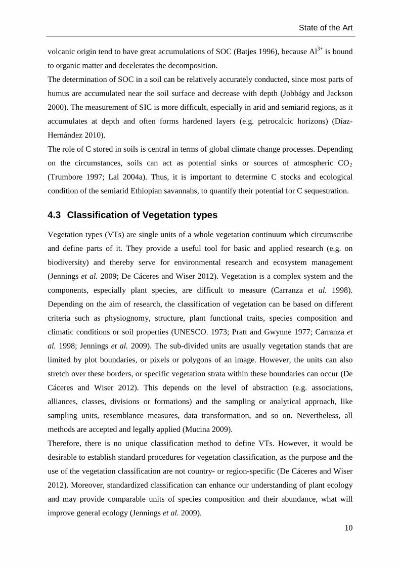
Two main characteristics are crucial for the determination of a VT; the definition of life form
and their dominance. The life form is the physiognomic appearance of a plant or a group of
plants, who have certain morphological characteristics in common (Küchler and Zonneveld
1988, cited in FAO 2005). Life form can be differentiated into woody plants, which are
further subdivided into trees and bushes, and herbaceous plants (forbs and graminoids). For
the distinction between trees and bushes, the height of plants can be used as a valid indicator.
To define the dominance, the main criterion is the highest canopy layer. Thereby, the
dominance follows the tree–bush–herbaceous layer. It is dependent on the cover of the
dominant life form. This means, that the dominant life form has to have a cover of either
“closed” or “open”. If the cover is only sparse, the dominance is subjected to another life form
whose cover is “closed” or “open” (FAO 2005) (Figure 3). In addition, a further subdivision
of the physiognomic term can be made in terms of species composition (Pratt and Gwynne
1977).
1 Flexibility in this context means, to enable the classification system to describe sufficient classes to cope with the real world. In addition, class boundary definitions should be unambiguous and clear. At the same time, however, classes have to be as neutral as possible in describing the vegetation type, to be feasible for a variety of end-users and disciplines (FAO 2005)
State of the Art
12
Further classifiers, that can be used to determine a VT more precisely, are Macropattern and
Stratification, however they will not be further described (for more information see FAO
2005).
Figure 3 Main structural Vegetation Domains (Di Gregorio and Jansen 1996, in FAO 2005)
The research on current vegetation in Ethiopia is of crucial importance, as the natural
vegetation has been modified through human influence, and there remain only a few patches
of natural vegetation communities (Woldu et al. 1989). The description of dominant VTs of
the Borana Plateau, and the link to their respective C stocks above- and belowground, will
provide a baseline for upscaling methods to predict C sequestration potential of broader areas.
4.3.1 Typical Grassland/Savannah vegetation In general, savannahs are defined by the co-existence of trees and grasses (Scholes and Archer
1997). The distribution of these two contrasting life forms, and their density, cover and
height, are essential for the understanding of general functions and processes of savannah
ecosystems (Sankaran et al. 2004). The forming and dominance of either woody or
herbaceous vegetation in a savannah ecosystem, is highly influenced by a number of
interacting factors such as climate, soil properties, resource competition, fire and grazing,
State of the Art
13
operating at different spatial and temporal scales (Scholes and Archer 1997). In addition, the
impact of human activity is nowadays an important driver and determining factor for the
existence of particular plant life forms. According to Pratt and Gwynne (1977) and White
(1983), major VTs of east African savannahs are presented below.
Woodland
Woodland is land with an open stand of trees up to
20 m in height, and which cover more than 20%.
The canopies of the trees are often in contact, but
are not densely interlaced (Figure 4b). If
shrubs/bushes are present, they count for less than
10% of the total cover. The ground cover is
dominated by grasses and other herbs.
Bushland
Bushland is land, dominated by bushes or trees
with a shrubby habit, usually between 3 and 7 m,
which is covered by at least 40%. Bushy trees up to
10 m in height and some occasional emergents can
be present as well (Figure 4a). If bigger trees are
more frequent within the bushland, the term
“wooded bushland” can be used. In general,
subtypes are classified respective to the genera of
the dominant woody plants. The herbaceous ground
cover is usually poor. Bush land thicket is and
extreme form where the bushes build a closed stand
and passing-through is difficult.
Shrubland
Shrubland is land, which is covered by more than 20% shrubs up to 6 m (often less). Trees are
seldom but can occur at a maximum of 10% of the total cover (Figure 4c). The ground cover
depends highly on the rainfall and the soil condition. With sufficient rainfall, grasses are
dominant on deep sandy soils, while stony and rocky places are favored by woody plants.
Comparably, as in bush lands, shrub land thickets can be recognized, too.
Figure 4 Physiognomic vegetation types. a) Bushland; b) Woodland; c) Shrubland; d) Bush grassland; e) Wooded grassland (i: tall wooded grassland; ii: dwarf tree grassland); f) Dwarf shrub grassland (Pratt and Gwynne 1977)
State of the Art
14
Grassland
In this VT, grasses and other herbs are the dominant life forms, with the former more
frequent. Occasionally, trees, bushes and shrubs are present widely scattered or grouped.
However, their canopy must not exceed 2% of the total cover; otherwise they are classified as
“wooded/bush/shrub grassland” (see below). Sub-types of grasslands are classified with
respect to their height (if it is not in the range of 25-150 cm), genera of dominant grasses,
degree of swampiness or the dominance by annual grasses or other herbs.
Tree grassland or wooded grassland
This refers to grasslands with scattered or assemblies of trees, with a canopy cover lower than
20% of the total surface.
Bush grassland
Bush grassland is defined by the presence of scattered or grouped trees and shrubs in
grasslands. Normally they occur with different amounts, but both are always conspicuous, and
together, they cover not more than 20% (Figure 4d). Sub-types are classified according to the
grassland type and the genera of the dominant woody plants. This includes grass height, the
dominance of annuals, dominant genera (grass/woody plants) and the degree of swampiness.
(Dwarf) Shrub grassland
Shrub grasslands are grasslands which consist of scattered or grouped shrubs with a canopy
cover of less than 20% of the area. For the classification of sub-types, the same criteria exist
as for bush grasslands (see above). A special type form dwarf shrub grasslands. These are
defined by often sparse grasslands with usually dwarf shrubs at a maximum of 70 cm in
height. Bigger shrubs are occasionally widely scattered. The term “dwarf” refers to all
vegetation types, where shrubs and trees are smaller than 70 cm and 2 m, respectively.
4.4 Dependence of carbon stocks on vegetation and species composition
Savannah ecosystems count to the most extensive C4 grassy biomes. Usually, they form
“patchy mosaic landscapes” with a relatively continuous cover of grass and herbaceous
vegetation and patches of scattered or grouped trees and/or bushes (Scholes and Archer 1997).
Woody plant invasion is an ongoing process (Jackson et al. 2002), which is the extension of
woody species into grasslands and savannahs. With the obvious change in vegetation
aboveground, the changes belowground are less conspicuous, but equally important. The
State of the Art
15
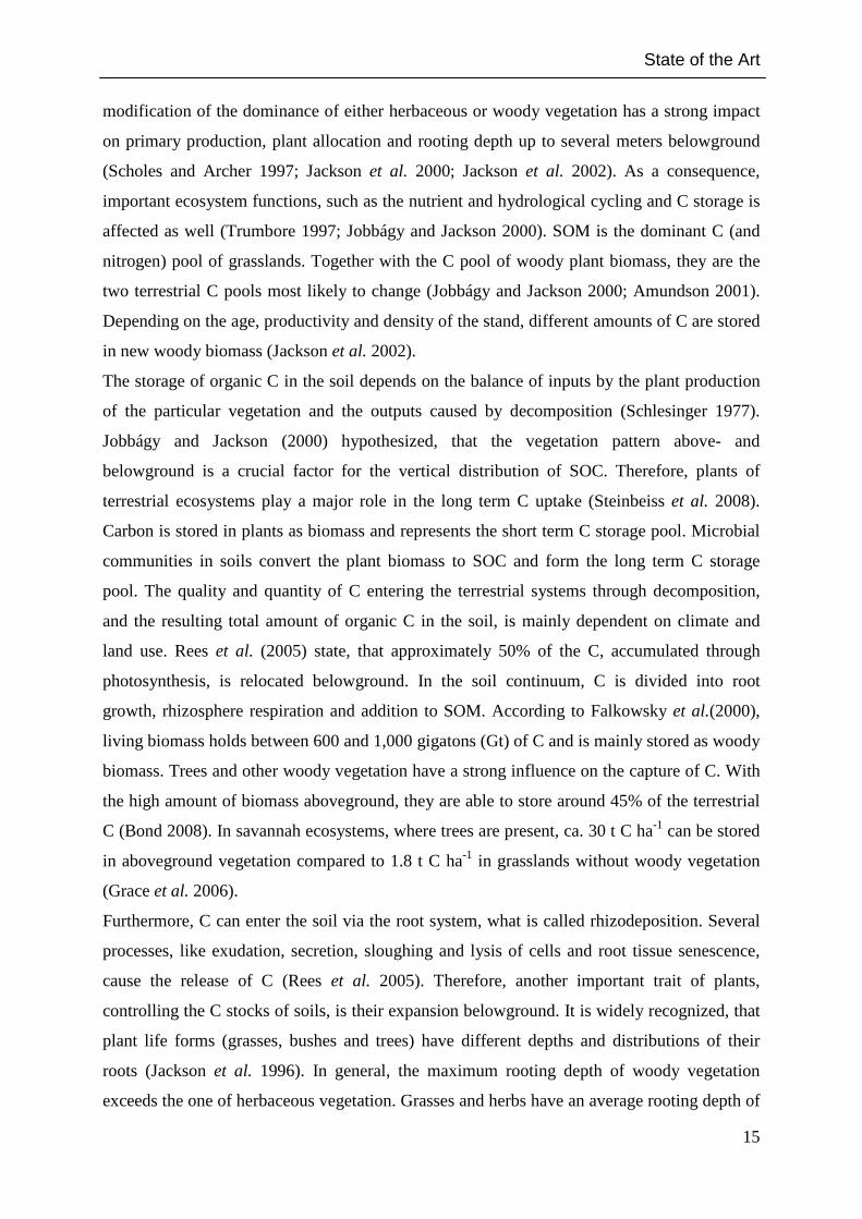
modification of the dominance of either herbaceous or woody vegetation has a strong impact
on primary production, plant allocation and rooting depth up to several meters belowground
(Scholes and Archer 1997; Jackson et al. 2000; Jackson et al. 2002). As a consequence,
important ecosystem functions, such as the nutrient and hydrological cycling and C storage is
affected as well (Trumbore 1997; Jobbágy and Jackson 2000). SOM is the dominant C (and
nitrogen) pool of grasslands. Together with the C pool of woody plant biomass, they are the
two terrestrial C pools most likely to change (Jobbágy and Jackson 2000; Amundson 2001).
Depending on the age, productivity and density of the stand, different amounts of C are stored
in new woody biomass (Jackson et al. 2002).
The storage of organic C in the soil depends on the balance of inputs by the plant production
of the particular vegetation and the outputs caused by decomposition (Schlesinger 1977).
Jobbágy and Jackson (2000) hypothesized, that the vegetation pattern above- and
belowground is a crucial factor for the vertical distribution of SOC. Therefore, plants of
terrestrial ecosystems play a major role in the long term C uptake (Steinbeiss et al. 2008).
Carbon is stored in plants as biomass and represents the short term C storage pool. Microbial
communities in soils convert the plant biomass to SOC and form the long term C storage
pool. The quality and quantity of C entering the terrestrial systems through decomposition,
and the resulting total amount of organic C in the soil, is mainly dependent on climate and
land use. Rees et al. (2005) state, that approximately 50% of the C, accumulated through
photosynthesis, is relocated belowground. In the soil continuum, C is divided into root
growth, rhizosphere respiration and addition to SOM. According to Falkowsky et al.(2000),
living biomass holds between 600 and 1,000 gigatons (Gt) of C and is mainly stored as woody
biomass. Trees and other woody vegetation have a strong influence on the capture of C. With
the high amount of biomass aboveground, they are able to store around 45% of the terrestrial
C (Bond 2008). In savannah ecosystems, where trees are present, ca. 30 t C ha-1 can be stored
in aboveground vegetation compared to 1.8 t C ha-1 in grasslands without woody vegetation
(Grace et al. 2006).
Furthermore, C can enter the soil via the root system, what is called rhizodeposition. Several
processes, like exudation, secretion, sloughing and lysis of cells and root tissue senescence,
cause the release of C (Rees et al. 2005). Therefore, another important trait of plants,
controlling the C stocks of soils, is their expansion belowground. It is widely recognized, that
plant life forms (grasses, bushes and trees) have different depths and distributions of their
roots (Jackson et al. 1996). In general, the maximum rooting depth of woody vegetation
exceeds the one of herbaceous vegetation. Grasses and herbs have an average rooting depth of
State of the Art
16
2-2.5 m, while trees and shrubs are found to have a rooting depth of 5 and 7 m on average
(Canadell et al. 1996). Grasses have a dense fibrous root system, which allows them to
explore the soil more intensively than it is the case for tree roots. In contrast, trees are able to
scan the soils more extensively and to a larger extend. So, they find high-resource patches
which are not occupied by grasses (Bond 2008). This can be explained by the specific root
length of the different vegetation life forms. Jackson et al. (1997) found, that grasses had
higher specific root length than any other life form (grasses: 118 m g-1; shrubs: 30 m g-1; trees:
12.2 m g-1). Fine roots are an important sink for C gained in net primary productivity, and the
primary production stored belowground often exceeds the one aboveground (Jackson et al.
1997). This leads to a higher input of C into the soil in grasslands compared to woodlands.
Further, the root:shoot ratio of the different vegetation forms is central for the C allocation
above and belowground. According to Jackson et al. (1996), root:shoot ratios of grassland are
in the range of 4 to 6, while the range for woodlands is much smaller.
The distribution of soil nutrients within the soil profile is another factor influenced by the
different vegetation life forms. Jackson et al. (2002) assessed that SOC is more deeply
distributed at sites with woody vegetation cover. 60 % of SOC was stored in the depth from 1
to 3 meters in woodland compared to 40 % in grasslands. However, if only the first meter of
soil is considered, the allocation of C is the other way round. Here, only one-fifth of the C
amount of grasslands is stored in woodlands.
Nevertheless, not only the plant life form of ecosystems, but also the diversity of plants and
community composition is found to be an important factor in increasing C storage in soils
(Catovsky et al. 2002; Fornara and Tilman 2008; Sebastia et al. 2008).
The impacts of plant diversity on litter decomposition derive from litter mixing effects and
through the building of a micro climate (Catovsky et al. 2002). Plant species diversity and
composition is able to enhance net storage of C and N in soils in two main ways; first through
a higher amount of C and N, that is entering the soil, and second through a decrease of their
losses via respiration, volatilization and leaching (Catovsky et al. 2002; De Deyn et al. 2008).
Fornara and Tilmann (2008) stated that the diversity effects on primary productivity in
grasslands depend heavily on the presence of N-fixing legumes. In prairie grasslands on sandy
soil with N being the limiting factor, they found out, that plant diversity increased the
accumulation of C and N. This was mainly because of the co-existence of C4 grasses and
legumes. N inputs were improved by the legumes, what facilitates the growth of C4 grasses
and caused N retention. These findings are further supported by Steinbeiss et al. (2008), who
observed higher soil C pools under higher plant species richness. In addition, the C:N ratio of
State of the Art
17
a plant community affects the decomposition rate (Dubeux Jr et al. 2006). The smaller the
C:N ratio, the higher the amount of N, the higher the rate of decomposition, and the higher the
amount of C in the soil. Thus, with greater species diversity, i.e. including N-fixing legumes,
the amount of C restored in the soil increases.
4.5 The role of Grasslands in carbon sequestration
“…Grasslands store about 343 billion tons of C – nearly 50 percent more than is stored in
forests worldwide.” (FAO 2010)
The term “soil carbon sequestration” refers to the removal of CO2 from the atmosphere by
plants and the storage in varying C pools, and is calculated in the timespan of a year (Lal
2001b; Lal 2004b). The resulting effects are increased SOC density in the soil, improved
distribution of SOC with depth and the stabilization of SOC through incorporation in micro-
aggregates (Lal 2004b). Terrestrial ecosystems in general have a great potential in
sequestering C for the mitigation of increased atmospheric CO2. However, grasslands in
particular hold a considerable amount of the world’s SOC, due to their vast expansion. About
52.5 million km² or 40.5 % of the Earth’s surface are covered by grassland ecosystems in a
wider sense (Suttie et al. 2005). In a narrower sense, tropical savannah ecosystems have a
share of 20 % of the terrestrial area (Neely et al. 2009). This suggests that these ecosystems
make a significant contribution in the global C cycle.
In grasslands, more C is stored in the soil than in the vegetation. White et al. (2000) point out,
that 231 Gt of C are stored aboveground compared to 579 Gt C in the soil under grasslands.
Conversely, forests store more C in their aboveground biomass (trunk, branches, and leaves)
than in the soil.
Land use change, especially the conversion of grasslands and pasture into cropland, counts to
the most important contributors of C emissions from the soil to the atmosphere. It is assumed,
that 5.5–6 Gt CO2 could be technically mitigated through adjusted management in
agriculture. Thereof, 1.5 Gt CO2 is from grazing land management, 0.6 Gt from restoration of
degraded land and >1.5 Gt from cropland management. Almost 70% of this potential can be
achieved in developing countries (IPCC 2007a). Further, Tennigkeit and Wilkes (2008)
estimate that improved rangeland management alone has the biophysical potential to sequester
1.3–2 Gt CO2 until 2030, globally.
Smith et al. (2008) lists a few integrated management interventions to reduce GHG emissions
and to increase C sequestration in grassland ecosystems. The most important are: (i)
State of the Art
18
managing grazing intensity, (ii) fire management, (iii) restoration of organic soils and
degraded lands and (iv) extending the use of perennial crops.
In addition, these management practices in grasslands will not only enhance the potential for
C sequestration, but it will have beneficial effects for ecosystem services, like greater
biodiversity, better water-holding capacity of the soil, and reduced soil erosion, and further
increases food production. By accomplishing a good management, grassland soils will still
sequester C for up to 50 years (Lal et al. 1998; Conant et al. 2001), which results in the
mitigation potential of 4–9% CO2-emissions in Africa per year (Batjes 2004). Batjes (2004)
further estimated that taking just the grasslands in Africa, improved management practices on
only 10 % of the area, soil C stocks could be increased by 1,328 million tons C per year in the
next 25 years.
Degradation of dry land pasture soils led to notable reductions of SOC during the last
decades. However, through the restoration of grasslands these lands will act again as C sinks
via the fixation of atmospheric CO2 on one hand and via reduction of erosion-induced CO2
loss on the other. Furthermore, the C loss in dry soils is smaller compared to wet soils due to
longer residence times and reduced decomposition (Neely et al. 2009). Therefore, grasslands
in dry lands of the world are essential for long-term C storage.
Thus, world’s grasslands yet play an important role in balance of atmospheric CO2 and in
addition hold a great potential for future mitigation practices if they are managed in an
equitable way.
Materials & Methods
19
5 MATERIALS & METHODS
5.1 Study area
The study was conducted in South Ethiopia, Oromia Region, Borana Zone. The experimental
site comprises a 10 km² field (NW: N4°16.682/E38°15.634; NE: N4°15.028/E38°20.853;
SW: N4°11.491/E38°14.058; SE: N4°9.868/E38°19.220), close to the Kenyan border
(Moyale) (Figure 5). The Borana Plateau covers a total area of 95.000 km². Around 350.000
inhabitants live in this region keeping about one million cattle, small ruminants and camels
(Homann et al. 2008). The landscape is characterized by moderately undulating hills with an
altitude of about 1.000–1.5000 m a.s.l. and may reach elevations up to 2.000 m a.s.l.
(Coppock 1994).
Figure 5 Map of the Research Area and Study Site location between Dubuluk and Mega, Borana Region, Southern Ethiopia (http://www.africa.upenn.edu/eue_web/borz0200_map.jpg, modified)
5.1.1 Climate The climate is characterized as semi-arid. The amount of annual rainfall shows great
differences with location and varies between 110 mm/year in the south and 600 mm/year in
the north. Rainfall shows a bimodal pattern (Figure 6). Between March and May,
approximately 60% of annual rainfall (main rainy season) occurs, 30% follow between
September and November (short rainy season) (Homann et al. 2008). In contrast, temperature-
variations are not so significant, as mean annual temperature varies between 15°C and 24°C
with only little seasonal changes. Long lasting droughts occur regularly every 20 years, while
isolated dry years occur every 5 years (Coppock 1994). However, the time span between
droughts is decreasing and the drought in 1999/2000 took place just 3 years after the previous
one (Homann 2004).
Figure 6 Climate chart of the study area (ILCA, unpublished data)
5.1.2 Agro-ecological zones Ethiopia has a wide range of temperature and rainfall pattern. As shown in Figure 7 the
country is divided into 17 agro-climatic zones based on a combination of six altitude layers
(ranging from <500 m a.s.l. to >3700 m a.s.l.) and three rainfall categories (Dry: <900
mm/year; Moist: 900–1400 mm/year; Wet: >1400 mm/year) (RELMA in ICRAF 2005). The
study area is lying at around 1500 m a.s.l. with an annual average rainfall of less than 900
mm. Therefore it forms a transition zone between “Dry Kolla” and “Dry Weyna Dega”.
Bereha Kolla
Weyna-Dega
Dega Wurch Alpine Wurch
< 500 m 500 – 1500 m
1500 – 2300 m
2300 – 3200 m
3200 - 3700 m > 3700 m
Dry
< 900 mm Dry
Bereha Dry
Kolla
Dry Weyna-
Dega
Dry Dega
Dry Wurch
Dry Alpine Wurch
Moist
900-1400 mm Moist Bereha
Moist Kolla
Moist Weyna-
Dega
Moist Dega
Moist Wurch
Moist Alpine Wurch
Wet
> 1400 mm Not existing Wet
Kolla
Wet Weyna-
Dega
Wet Dega
Wet Wurch
Wet Alpine Wurch
Figure 7 Agro ecological zones of Ethiopia (RELMA in ICRAF 2005)
Materials & Methods
21
5.1.3 Geology and Soils Soils of the Borana Plateau are influenced by four geological formations: (1) Precambian
basement complex and crystalline rocks which comprises granite, gneisses and magmatite, (2)
sedimentary deposit like sand stone and lime stone, (3) volcanic basalt and tuff and (4)
quaternary deposit, namely alluvial deposit and alluvial-in situ weathering rock (Oromiya Soil
Survey Report, unpublished).
Important soil forming factors of the area were climate, parent material, relief/topography,
organisms (flora and fauna) and human activity. A combination and interaction of these
factors led to different soils and their characteristics. Parent material has to be emphasized in
soil development, because various soil minerals will result from the break down under
weathering of different rocks. The breakdown of basaltic rocks results in forming clay
textured soil, while the breakdown of granite and gneiss results in a sandy, sandy loam, loamy
and sandy clay loam texture (Oromiya Soil Survey Report, unpublished).
Major soil types found in the study area were Cambisols, Vertisols and Calcisols. Cambisols
are relatively young soils and typical for temperate zone, but occur in tropical regions as well
(WRB 2006). Colors varied from reddish-brown to white brown and brown. Vertisols are
typical soils of the seasonal tropics and subtropics, mainly in regions with changing rainfall
amounts. Due to their high amount of clay, with ability to swelling and shrinking, they are
very sticky when wet and hard when they dry out, forming deep cracks in the dry season. In
the study area, they were found in depressions and their color varied from dark brown to dark
grey. Calcisols are common in arid and semi-arid areas and occur mainly on highly calcareous
parent material (Oromiya Soil Survey Report, unpublished). Calcisols identified in the study
area were white-grey-brownish and had a loamy texture. (Soils of the study area and their
properties see Appendix I)
5.1.4 Vegetation Native vegetation of the Borana Plateau is composed of diverse mixtures of woody and
herbaceous vegetation and is therefore characterized as tropical savannah (Pratt and Gwynne
1977). Important characteristics of savannah systems are their variation in proportion of
woody and herbaceous material and drastic composition shifts due to heavy grazing,
browsing, fire and severe droughts (Northon-Griffiths, 1979; Walker and Noy-Meir, 1982,
cited in Coppock 1994). It is assumed, that grazing might favor trees whereas browsing rather
promotes grass vegetation (Walker and Noy-Meir, 1982, cited in Coppock 1994). Coppock
(1994) hypothesizes, due to heavy grazing and the absence of fire perennial woody plants are
dominating many plant communities. 5-75% of total plant cover in Borana consists of
Materials & Methods
22
perennial woody plants (Coppock 1994). An essential feature of perennial plants in this area is
their persistence, because of the bimodal uncertain pattern of rainfall. Even small rainfall
events can induce greening. In addition, their permanent rooting system is a good prevention
against erosion (Ukkerman, 1991, cited in Coppock 1994).
Dominant tree species found in the area were Acacia tortilis, A. nilotoca, A. bussei and A.
seyal. Bush and shrub species identified were mainly A. mellifera, A. drepanologium and A.
nubica often associated with Solanum ssp. and Ocimum ssp. Grasslands showed a wide range
of species composition depending on the site factors and soil type. Pennisetum ssp. was
mainly found on Vertisols and soils with a good water holding capacity. On other soil types a
mixture of annual and perennial plants was identified. Sporobulus ssp., Eragrostis ssp.,
Cenchrus ciliares L., Cynodon dactylon L. and herbaceous plants like Crotalaria ssp and
Bidens ssp. were dominating these areas.
5.1.5 Land Use The traditional land use system of the Borana zone was a pastoral system characterized by
cattle grazing and browsing by sheep, goats and camels (Oromiya Soil Survey Report,
unpublished). As surface water was only seasonally available, rainy season grazing was
dominant (Homann et al. 2008).
Since the 1970, research and development efforts to improve rangeland productivity led to a
transition from traditional pastoralism to semi-sedentary grazing systems. Major changes
resulting in this modification were (i) the construction of additional watering ponds, causing
permanent settlement within formerly seasonal pastures and the possibility for year-round
grazing, (ii) the official prohibition of burning and (iii) increasing crop cultivation due to
extension services (Homann et al. 2008).
5.2 Experimental Setup
5.2.1 Determination of representative vegetation types (VTs) To get an overview of the natural vegetation and plant communities that are most representing
the area, first of all the study area was surveyed by foot. With the help of a “Google Earth”
satellite image, prominent vegetation cover was determined visually. By ground-trouthing in
North-South and East-West direction, the vegetation cover and current plant communities
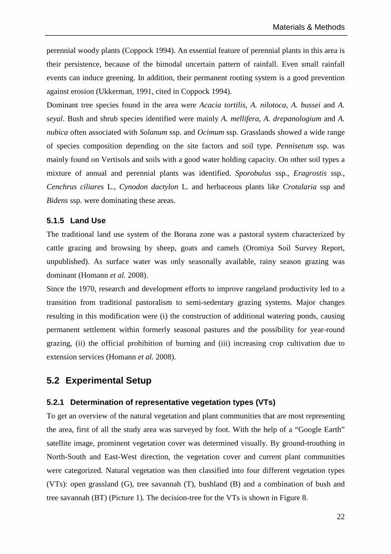
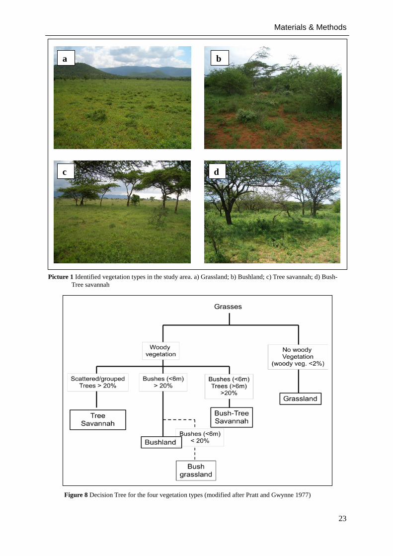
were categorized. Natural vegetation was then classified into four different vegetation types
(VTs): open grassland (G), tree savannah (T), bushland (B) and a combination of bush and
tree savannah (BT) (Picture 1). The decision-tree for the VTs is shown in Figure 8.
Materials & Methods
23
a b
Picture 1 Identified vegetation types in the study area. a) Grassland; b) Bushland; c) Tree savannah; d) Bush-Tree savannah
Figure 8 Decision Tree for the four vegetation types (modified after Pratt and Gwynne 1977)
c d
Materials & Methods
24
5.2.2 Site selection Representative plots were selected by visual observation and with the help of a satellite image
(googleearth.com). For the visual observation, small hills within and bordering the study area
were climbed to get an overview and pictures were taken in every geographic direction. After
that, these pictures were analyzed and compared to the satellite image. Possible locations of
the searched VT were marked in the satellite image to get the GPS coordinates. Using a GPS
(60CSx Garmin, USA), the preselected locations were visited and discussed if they match
with the classified VT in terms of vegetation cover, species composition and stand density. If
the criteria were fulfilled, the plot was chosen for further investigation.
5.2.3 Plot and Sampling design Overall, twenty 900 m² sample plots were established, representing 5 plots per VT. GPS
coordinates of each selected sampling plot were taken with a GPS (60CSx Garmin, USA) and
mapped within the satellite image as shown in Figure 9a.
Each of the 900 m² plots used for field measurement had the same sampling design (Figure
9b). As tree stand densities were generally very low in this area, a plot size of 30x30 m was
chosen to include at least three trees per plot in the “trees savannah” VT. In order to better
connect the outcome with each other, the investigated plots of the different VTs had all the
same size. For the destructive measurement and species identification of understorey
vegetation (mainly grass and small herbaceous vegetation) five subplots with a size of 1x1 m
were established along two diagonal lines in the plot.
Using a Puerckhauer auger, 10 randomized soil samples of one meter depth were taken within
the 900 m² plots. Soil bulk density was measured at two different positions in each plot in two
different depths (0-10 cm and 10-30 cm, respectively).
Materials & Methods
25
Figure 9 Plot and sampling design. (a) Distribution of the sampled plots within the 10 km² study area and (b)
Sampling design of each 30 m² Plot.
5.2.4 Soil sampling Soil samples were taken once before and once after the
rainy season to display seasonal changes. Ten randomly
chosen auger points were taken within the five plots of
every of the four different VTs, using a Puerkhauer auger
up to one meter depth if possible, or until the parent
material was reached (Picture 2). The samples were
separated in four different depth: (a) 0-10 cm, (b) 10-30
cm, (c) 30-60 cm and (d) 60-100 cm and filled into a
labeled plastic bag. The samples were used for laboratory
analysis of total carbon (TC), SOM, soil organic carbon
(SOC), pH and carbonate (CaCO3) content. In addition
one auger point was used for soil type identification to
describe texture, color and carbonate content after using a
Munsell chart and HCl acid.
5.2.5 Bulk density For the determination of soil bulk density (BD), two 40 cm deep holes were dug at two
different positions in each of the 20 plots. Any place with soil compaction, e.g. due to foot
trails, was avoided. In two different depths (0-10 cm and 10-30 cm) standardized coring
cylinders with a volume of 100 cm³ were pushed into the soil vertically using a rubber
hammer and a block of wood (Picture 3). The sampling needed to be carried out carefully, to
= Augerpoints
a) b)
Picture 2 Puerkhauer auger and soil sampling equipment
Materials & Methods
26
avoid any disturbance of the soil. The coring cylinder,
containing the soil, was then dug out of the soil using a
spatula. Excess soil was removed from both sides of the
coring cylinder with a knife and the cylinders were closed
with a plastic cap. For transport, the soil was filled into a
plastic bag and labeled with the respective ID. In every plot
five replications per depth were taken (n=200).
5.2.6 Sampling of vegetation (destructive/non-destructive) At all sampling locations, observed site factors, like closeness to a village or foot trails,
elevation and GPS coordinates were recorded. Trees and bushes were documented in a map
and species were identified with the help of a local expert.
5.2.6.1 Trees
All sampled trees within the plot (900 m²) were numbered and their location recorded in a
map. For estimating the tree biomass of each tree, allometric equations from literature were
used. Therefore, circumference at breast height (1,3 m) (DBH), basal circumference at 0,3 m
from ground (D30), stem height (HS), total tree height (HT), height at lower end of canopy
(HC), tree crown width (CW) and length (CL) were measured.
Stem height and circumferences in the two heights were measured using a measuring tape.
Some measured trees were odd-shaped at measuring height, e.g. forking trees or bulging trees.
These trees were measured according to Hairiah et al.(2001) (Figure 10).
Figure 10 Measuring procedure on odd-shaped trees (Hairiah et al. 2001)
Total tree height and height at lower end of canopy were measured using a wooden stick of
seven meters, marked with colored tape at 50 cm intervals. The stick was lifted until the end
Picture 3 Bulk density sampling
Materials & Methods
27
matched with the top of the canopy (Picture 4a). The missing centimeters were measured with
a ruler and added to the seven meters of the stick.
Canopy width and length were measured with a measuring tape by two persons standing at the
margins of the canopy in two orthogonal directions (Picture 4b). Canopy diameter (Cd) was
then calculated as the average of CW and CL. Ground cover was calculated with the circle
area:
𝐶𝑖𝑟𝑐𝑙𝑒 𝐴𝑟𝑒𝑎 [𝑚2] = 𝜋 × (𝐶𝑑)² 4⁄
Picture 4 Tree height (a) and crown width and length (b) measurement
Aboveground biomass of trees was then calculated using allometric equations below:
For Acacia tortilis, A. bussei and A. nilotica (Hofstad 2005)
𝑌 = 0,0096 × (𝐻𝑇 + 𝐶𝑤 + 𝐶𝐿)3,3015
Where HT is total height [m], CW is crown width [m] and CL is crown length [m].
For A. drepanolobium (Okello et al. 2001)
𝑌 = 3,77 × 𝐷30 + 1,1682
Where D30 is basal diameter at 0.3 m from ground [cm].
5.2.6.2 Bushes/Shrubs
The sampling of bushes was similar to trees. The position of every bush/shrub was recorded
in a map and they were classified into three different size categories (small/medium/big),
defined through visual observation. Due to early branching, and a dense habitus, only the
basal circumference (D30) at 0.3 m from the ground was measured, using a measuring tape.
Further, the canopy width (CW) and length (CL) were measured in the same way as it was
done for trees (see section 5.2.6.1). Bush height (HB) was estimated using a wooden stick,
marked with colored tape at 50 cm intervals, standing next to the bush. Three bushes of every
a b
Materials & Methods
28
size category and of every different species were randomly chosen for measurement. The
amount of aboveground biomass of every bush was calculated using the following formula:
For A. mellifera and A. nubica (Hofstad 2005)
𝑌 = 0,0548 × (𝐻𝑇 + 𝐶𝑤 + 𝐶𝐿)2,5767
Where HT is total height [m], CW is crown width [m] and CL is crown length [m].
For Ocimum ssp., Lantana ssp. and Solanum ssp. (Sah et al. 2004)
𝑌 = 0,446 × 𝐶𝐴0,869 × 𝐻𝑇1,112
Where CA is Circle Area [m2] and HT is total height [m].
The average of the different size categories and species was calculated and upscaled for the
whole plot corresponding to the number of species.
5.2.6.3 Species composition
Five subplots along two diagonal lines were positioned in the main plot. Species composition
was classified with the help of a local expert. Total ground cover [%] and abundance of every
species [%] was estimated visually and recorded. The total number of species per plot was
determined as a parameter to measure biodiversity.
5.2.6.4 Harvest of understorey vegetation
For this destructive method, three subplots of 1 m² were established in the plot along a
diagonal line. All vegetation (mainly grasses, weeds and small shrubs) within the subplot was
cut at ground level packed in oven proof labeled paper bags and oven-dried at 65°C until
weight constancy (Picture 5). Subsequently, dry weight was recorded and averaged for the
three subplots. Potential dry matter production per hectare was calculated with the following
formula:
𝐷𝑀 [𝑔 𝑚−2] × 1000 = 𝐷𝑀[𝑘𝑔 ℎ𝑎−1]
Picture 5 Harvest of under storey vegetation, cutting and packing into oven proof paper bags
Materials & Methods
29
5.3 Laboratory Analysis
5.3.1 Organic carbon in the soil (belowground) Loss-on-Ignition (LOI) Method
Loss-on-Ignition is a common and often applied method to estimate soil organic matter
(SOM) content. During a burning process at 550°C, organic matter is oxidized to carbon
dioxide (CO2) and ash (Heiri et al. 2001) which can be measured by the weight loss of the
samples.
Soil samples were air dried, sieved (2 mm fraction) and then ball-milled for 3 minutes for a
complete homogenization. 5 g of soil were weighed into ceramic crucibles with a mass
balance (0.01 g). As most of the soils investigated were very clayey (> 40%) the samples were
oven dried at 180°C for 12 hours, to remove the crystalline water captured between the clay
particles (personal communication with Prof. Dr. K. Stahr). After drying, the crucibles with
the soil were weighed again and the moisture loss was recorded. Then, the samples were put
in a muffle furnace and heated up at 550°C for 4 hours (Kamau-Rewe et al. 2011). After
burning in the muffle furnace, the samples were put in a desiccator to avoid further water
enrichment while cooling down. Then the ash was weighed again and the weight loss was
recorded.
The soil organic matter and resulting soil organic carbon content were calculated as follows:
5.3.4 pH Measurement (after DIN 19684) For the pH measurement 3 out of 10 augers were randomly selected and the 4 depths (0-10
cm, 10-30 cm, 30-60 cm and 60-100 cm) were measured separately, accounting for a total
number of 12 measurements per plot and 240 for all 20 plots in different VTs.
5 g of air dried and sieved (2 mm) soil was mixed with 12.5 ml 0.01 M calcium chloride
(CaCl2) – solution. The samples rested for 3 hours and were stirred every 30 min using a glass
stirrer. Before measurement, the samples were stirred again. After coarse particles had settled
Materials & Methods
31
down, the pH-electrode was dipped into the supernatant. As soon as the pH value was
constant (≥30 s) it was noted at two decimal places.
Previous to every measurement, the pH-electrode has to be calibrated in the expected
measurement range with two different calibration solutions.
5.3.5 Carbonate Content (after DIN ISO 10693) Soil carbonate content was analyzed using Scheibler method. 2 to 5 g sieved (2 mm) and
oven-dried (105°C) soil samples were treated with 10% hydrochloric acid. Carbonates in the
soil react with the acid and the resulting CO2 can be measured.
With the following formula, the CaCO3 content was calculated:
% 𝐶𝑎𝐶𝑂3 = 𝑚𝑙 𝐶𝑂2 × 𝑚𝑚 𝐻𝑔 × 0,1605
(273 + 𝑡) × 𝐸
Where t is the ambient temperature [°C], E is the weight of the sample [g] and mm Hg is the
air pressure [mm Hg].
5.4 Statistical analysis
The statistical analysis was done with the statistical package SAS 9.3. A one-way ANOVA
was operated using the “mixed” procedure, to test for fixed and random effects. The data was
tested for normal distribution. If they were not normally distributed, they were transformed
using logarithms. Outliers were eliminated to achieve normal distribution. Level of
significance was set at p<0.05 and a t-test was applied to test for significant differences
between the means.
Graphs and diagrams were produced with the program Excel 2007.
In addition, a Cluster analysis was conducted using the program IBM SPSS Statistics 20. A
hierarchical model using Ward-Model (Minimum variance method) and with Euclidian
distance as similarity index, was applied.
Detailed data on SAS calculations are found in Appendix III.
Results
32
6 RESULTS
6.1 Aboveground biomass
Figure 11 Aboveground biomass [t ha-1] in the different vegetation types. Means with different letters are
significantly different at p<0.05. Bars represent the standard error of the mean. G = Grassland, B = Bushland, T = Tree savannah, BT = Bush-Tree savannah
Figure 11 shows the aboveground biomass (AGB) of the four different vegetation types
(VTs). AGB was significantly different (p<0.05) between the VTs. The Tree savannah (T)
had the highest AGB (51.9 ± 16.1 t ha-1), and was significantly different (p<0.05) from the
other VTs. Between the Bush-Tree savannah (BT) and Bushland (B), there were no
significant differences and an AGB of 24.0 ± 5.9 t ha-1 and 10.9 ± 0.9 t ha-1 was measured,
respectively. The lowest AGB was measured in Grasslands (G) with 0.8 ± 0.4 t ha-1, which
was significantly different (p<0.05) to the other VTs.
AGB was further divided into the different life forms within the VTs. The Biomass
Production of trees and bushes was dependent on the VT, as shown in Figure 12. The AGB of
bushes ranged from 3.15 ± 1.13 t ha-1 in BT to 9.55 ± 0.85 t ha-1 in B. The amount of AGB in
bushes was significantly higher (p<0.05) in B. Tree biomass was significantly higher in T
compared to BT, ranging from 19.27 ± 5.9 t ha-1 in BT to 50.98 ± 16.09 t ha-1 in T. Grass
production ranged from 0.96 to 1.40 t ha-1 and showed no significant differences among the
VTs.
c
b
a
b
0
10
20
30
40
50
60
70
G B T BT
Abov
e gr
ound
bio
mas
s [t
ha-1
]
Vegetation Type
Aboveground biomass [t ha-1]
Results
33
Figure 12 Aboveground biomass [t ha-1] in different vegetation life forms within the four VTs. Means with
different letters and the same color are significantly different at p<0.05. Bars represent the standard error of the mean. G = Grassland, B = Bush land, T = Tree savannah, BT = Bush-Tree savannah
6.2 Carbon stocks
6.2.1 Aboveground Carbon stocks Mean aboveground carbon stocks [t ha-1] of the different VTs are shown in Figure 13 (G, 0.4
± 0.2 t C ha-1; B, 5.5 ± 0.4 t C ha-1; T, 25.9 ± 8.1 t C ha-1; BT, 11.9 ± 2.9 t C ha-1).
Figure 13 Aboveground carbon stocks [t C ha-1] in the different vegetation types. Means with different letters
are significantly different at p<0.05. Bars represent the standard error of the mean. G = Grassland, B = Bushland, T = Tree savannah, BT = Bush-Tree savannah
a b
a
b
0
10
20
30
40
50
60
70
G B T BT
Abov
e gr
ound
bio
mas
s [t
ha-1
]
Vegetation Type
Aboveground biomass in the vegetation life forms [t ha-1]
Grass
Bush
Tree
c
b
a
ab
0
5
10
15
20
25
30
35
G B T BT
AGC
S [t
C h
a-1 ]
Vegetation Type
Aboveground carbon stocks [t C ha-1]
Results
34
The aboveground carbon stocks (AGCS), stored in the vegetation, were different between the
VTs in the order G<B<BT<T. T showed the highest AGCS. The AGCS of T were
significantly higher (p<0.05) than those of B and G, but were not significantly different to BT.
G and B also showed significant differences in AGCS (p<0.05). Between B and BT no
significant differences were measured.
When looking at the different vegetation life forms (Figure 14), carbon allocation differed
significantly among the VTs. Carbon accumulated in the bushes ranged from 1.58 ± 0.57 t C
ha-1 in BT to 4.77 ± 0.32 t C ha-1 in B. The amount of C in trees was 25.49 ± 8.07 t C ha-1 in T
and 9.63 ± 2.97 t C ha-1 in BT. Corresponding to the AGB (Figure 12), significantly more
Carbon (p<0.05) was stored in bushes of B than BT, and significantly more in trees of the T
compared to BT (p<0.05).
Figure 14 Aboveground carbon stocks [t C ha-1] in the different vegetation life forms within the four vegetation
types. Means with different letters and different colors are significantly different at p<0.05. Bars represent the standard error of the mean. G = Grassland, B = Bushland, T = Tree savannah, BT = Bush-Tree savannah
6.2.2 Belowground carbon stocks Figure 15 shows the mean soil organic carbon (SOC) concentration in percent of the different
VTs. SOC (%) ranged from 2.93 ± 0.27 % in B, over 3.22 ± 0.49 % and 3.22 % ± 0.25 % in G
and T, to 3.26 ± 0.33 % in BT. However, the difference in SOC [%] between the VT was not
significant (p<0.05).
a b
a
b
0
5
10
15
20
25
30
35
G B T BT
AGCS
[t C
ha-1
]
Vegetation Type
Aboveground carbon stocks in the different vegetation life forms [t C ha-1]
Grass
Bush
Tree
Results
35
0,0
0,5
1,0
1,5
2,0
2,5
3,0
3,5
4,0
G B T BT
SOC
[%]
Vegetation Type
Soil organic carbon concentration [%]
Figure 15 Average soil organic carbon concentration [%] over 1m depth in the different vegetation types. Bars represent the standard error of the mean. G = Grassland, B = Bushland, T = Tree savannah, BT = Bush-Tree savannah
Figure 16 Soil organic carbon concentration [%] in four depths in the different vegetation types. Letters indicate
significant differences between soil depths of 10 cm depth within the same vegetation type at p<0.05. Bars represent the standard error of the mean. G = Grassland, B = Bushland, T = Tree savannah, BT = Bush-Tree savannah
SOC concentration [%] varied between 2.57 % and 4.15 % across the VTs and different
depths (Figure 16). VT had no significant influence on SOC concentration (p<0.05). Only soil
depth showed significant differences within the VT of B and T. In B the two first soil layers
(0-30 cm) and the layer 60-100 cm were significantly higher in SOC concentration (p<0.05)
than the soil layer (30-60 cm). Nonetheless, the differences between the layer 10-30 cm and
a c ab c
c b b
a
0
1
2
3
4
5
G B T BT
SOC
[%] p
er 1
0 cm
Vegetation Type
Soil organic carbon concentration [%] by depth
0-10 cm
10-30 cm
30-60 cm
60-100 cm
Results
36
60-100 cm were not significant (p<0.05). In T, SOC concentration increased significantly
with increasing soil depth. SOC concentration in the topsoil (0-30 cm) was significantly lower
(p<0.05) than the following layers and the concentration in layer 30-60 cm was significantly
lower (p<0.05) than the one in the deeper soil layer (60-100 cm).
Across the VTs, the first 60 cm showed no significant changes in SOC concentration
(p<0.05). As shown in Table 1, the SOC concentration of the subsoil were significantly higher
(p<0.05) compared to the other layers.
Table 1 Soil organic carbon concentration [%] in the four different depths. Means with different letters are significant different
Trait Treatment Depth Lsmean
transf.
Std error
transf.
Significance
(p<0.05)
SOC Depth 0 -10 cm 1.072 0.07361 b
10-30 cm 1.041 0.07361 b
30-60 cm 1.040 0.07363 b
60-100 cm 1.133 0.07415 a
Figure 17 Total soil organic carbon stocks [t C ha-1] up to 1m depth in the different vegetation types. Bars
represent the standard error of the mean. G = Grassland, B = Bushland, T = Tree savannah, BT = Bush-Tree savannah
In terms of total soil organic carbon stocks (SOCS) [t C ha-1] up to one meter depth, no
significant differences (p<0.05) were observed between the VTs. The amounts of carbon
stored in the soil in the first meter varied between 326.4 ± 28.6 t C ha-1 in B, 372.3 ± 44.8 t C
ha-1 in G, 374.4 ± 22.5 t C ha-1 in BT and 394.9 ± 22.0 t C ha-1 in T (Figure 17).
050
100150200250300350400450
G B T BT
SOC
S [t
C h
a-1 ]
Vegetation Type
Total soil organic carbon stocks [t C ha-1] up to 1 m depth
Results
37
Figure 18 Soil organic carbon stocks [t C ha-1] in four depths in the different vegetation types. Means of depths
within the same vegetation type with different letters are significantly different at p<0.05. Bars represent the standard error of the mean. G = Grassland, B = Bushland, T = Tree savannah, BT = Bush-Tree savannah
Within the VTs, SOCS [t C ha-1] varied on average from 29.60 t/ha to 48.27 t/ha in the
different soil layers per 10 cm depth (Figure 18). There were no significant differences
between the different VTs (p<0.05). Within B and T the significant differences occurred
between the different soil layers. In B there were no significant differences in the first 30 cm.
SOC stocks of the soil layer 30-60 cm were significantly lower than the soil layers 0-10 cm,
10-30 cm and 60-100 cm. However, there were no significant differences (p<0.05) between
the first 30 cm and the deeper soil layers (>60 cm). In T, again there were no significant
differences between the first and the second soil layer. In contrast to B, SOCS were
significantly higher in the soil layer 30-60 cm and in the deepest layer (60-100 cm) compared
to the first two layers. Across the VTs, there were no significant differences within the first 60
cm. The amount of SOC (t/ha) in the soil layer from 60-100 cm was significantly higher
(p<0.05) compared to all layers above (Table 2).
Table 2 Soil organic carbon stocks [t C ha-1] in the four different depths. Means with different letters are significantly different.
Figure 19 Seasonal change in SOC accumulation [t C ha-1] from dry season to rainy season. Means with
different letters within the same vegetation type are significantly different at p<0.05. Bars represent the standard error of the mean. G = Grassland, B = Bushland, T = Tree savannah, BT = Bush-Tree savannah
Figure 19 shows the changes in SOCS from dry season to rainy season. On average, SOCS in
one meter depth ranged from 339 to 383 t ha-1 in the dry season, while SOCS in the rainy
season ranged from 325 to 367 t C ha-1. Between the VTs, season had no significant influence
(p<0.05) on the carbon stored the in soil. Within the VTs, only in T significantly less SOC
was stored in the soil in the rainy season compared to the dry season.
Figure 20 and Figure 21 show the SOCS [t C ha-1] in two different depths (0-30cm and 30-
100cm, respectively). In the upper soil layer SOCS from 99-120 t C ha-1 in the dry season, and
96-109 t C ha-1 in the rainy season, were allocated. In deeper soil layers the SOCS ranged
from 236 to 280 t C ha-1 in the dry season and from 219 to 259 t C ha-1 in the rainy season.
Between the VTs no significant differences occurred in any depth. However, when looking at
the single VT, in the soil layer 0-30cm, significantly less (p<0.05) carbon was accumulated in
BT in the dry season than in the rainy season. Soil layer 30-100 cm showed significant
differences (p<0.05) between the seasons in B and T, where SOCS decreased from dry to
rainy season.
a b
050
100150200250300350400450
G B T BT
SOC
S [t
C h
a-1 ]
Vegetation Type
Change in SOC [t C ha-1] from dry to rainy season
Dry Season
Rainy Season
Results
39
Figure 20 Seasonal change in SOCS [t C ha-1] from dry season to rainy season in the soil layer 0-30 cm. Means
with different letters within the same vegetation type are significantly different at p<0.05. Bars represent the standard error of the mean. G = Grassland, B = Bushland, T = Tree savannah, BT = Bush-Tree savannah
Figure 21 Seasonal change in SOC stocks [t C ha-1] from dry season to rainy season in the soil layer 30-100 cm.
Means with different letters within the same VT are significantly different at p<0.05. Bars represent the standard error of the mean. G = Grassland, B = Bushland, T = Tree savannah, BT = Bush-Tree savannah
a
b
0
20
40
60
80
100
120
140
G B T BT
SOC
S [t
C h
a-1 ]
Vegetation Type
Seasonal change in SOC stocks [t C ha-1] 0-30 cm
Dry Season
Rainy Season
a
a
b b
0
50
100
150
200
250
300
350
G B T BT
SOC
S [t
C h
a-1 ]
Vegetation Type
Seasonal change in SOC stocks [t C ha-1] 30-100 cm
Dry Season
Rainy Season
Results
40
6.3 Species composition
A total of 72 species were identified in the research area, of which 28 were grass species and
belonged to the family of Poaceae. 44 species were herbaceous species and belonged to 22
different families. Trees and bushes identified in the area were Acacia species counting to the
family of Mimosaceae. Further, dominant shrubs were Grewia bicolor, Grewia villosa,
Lantana rhodesensis, Solanum somarense and Ocimum lamiifolium (Table 3).
Table 3 Habitus, Family and Distribution of species of the research area of the Borana Plateau, Ethopia
Species Habitus2 Family Vegetation type3 and Distribution1
G B T BT
Aristida adscensionis L. a Poaceae + Cenchrus ciliaris L. p Poaceae C P D P Cynodon dactylon L. p Poaceae P P P Chrysopgon plumulosus (L.) Pers. p Poaceae P C C P Chloris roxburghiana Schult. p Poaceae P Chloris virgata sw. a Poaceae Panicum coloratum L. p Poaceae P + P P Eragrostis papposa Ruem & Schult. Steud p Poaceae P + C C Eragrostis cilianensis (All.) Lutati a Poaceae + P P P Enneapogon cenchroides Ruem & Schult. C.E. Hubbard a Poaceae Leptothrium senegarense (Kuth.) p Poaceae + Microchloa kunthii esv. a Poaceae C + + Sporobulus pyramidlis P. Beauv. a Poaceae C C C C Sporobulus festivus A. Rich. a Poaceae P P Setaria varticillata (L.) P. Beauv. a Poaceae P P C Tragus berteronianus Schult. a Poaceae P + Tragus heptaneuron Clayton a Poaceae Brachiaria humidcola (Rendle) Schweick. a Poaceae P + C C Brachiaria eruciformis a Poaceae Pennisetum mezianum (Vahl.) Lanza Mattei p Poaceae D D P D Pennisetum stramineum Pete V. p Poaceae P P P Commelina latifolia A. Rich a Poaceae C C P C Commelina subulata Rott. a Poaceae P P Bothrichloa radicans A. Camus. p Poaceae + + Digitaria velutina Forssk. P. Beauv. a Poaceae + Tetrapogon cenchriformis (A. Rich) W.D. Clayton p Poaceae + Lintonia nutans, stapf. p Poaceae + P P P Dactyloctenium aegypticum (L.) Pers a Poaceae + P + P Sida ovata Forssk. a Malvaceae + + P P Becium verticillifolium beke cufed. p Lamiaceae + + P Ocimum basilicum L. a Lamiaceae P P + Ocimum lamiifolium Hocht.ex Benth. p Lamiaceae C D
Results
41
Portulaca oleracea L. a Portulaceae P + P + Bidens pilosa L. a Compositae + + Launaea cornuta (Hochst. ex. Oliv. & Hiern.) C. Jeffrey a Nyctalinaceae + P P Boerhaavia erecta L. a Compositae + + P Amaranthus graecizams L. a Amaranthaceae P P P Plantago lanceolata L. p Plantaginaceae + Erucastrum arabicum Fisch & Mey. a Compositae C P C C Anthemis tigreensis A. Rich a Compositae + + Crotalaria incana L. a Fabaceae P P P Crotalaria agatiflora subsp. engleri (Baker f.) Polhill a Fabaceae C + Indigofera spinosa Forssk. p Fabaceae C P + Indigofera volkensii Taub. p Fabaceae Helichrysum glumaceum D.C. a Asteraceae C P P Dyschoriste hildebrandtii (S.Moore) p Acanthaceae P P + C Achyranthes apera L. a Amaranthaceae P P Kyllinga bulbosa P. Beauv. a Cyperaceae P + + + Cyperus amauropus Steud. p Cyperaceae P + + Heliantropium cinrascens D.C. a Boraginaceae Tribulus terrestris L. p Zygophyllaceae Oxygonum sinuatum (Meisner) Dammer a Zygophyllaceae P + + + Psydrax schimperiana (A.Rich) a Rubiaceae + P C Chenopodium opulifolium Koch. a Chenopodiaceae + Acacia mellifera Vahl Benth. p Mimosaceae D C Acacia nubica Benth. p Mimosaceae C Grewia bicolor Juss. p Tiliaceae P Grewia villosa willd. p Tiliaceae P Lantana rhodesensis moldenke. p Verbenaceae P D Solanum incanum L. p Solanaceae P P P P Solanum giganteum Jacq. p Solanaceae Vernonia cinerascens Schultz Bip. p Asteraceae Solanum somarense Franchet p Solanaceae C C D Acacia seyal Del. p Mimosaceae P Acacia tortilis (Forssk.) Hay. p Mimosaceae D C Acacia nilotica (L.) Del. Var. Nilotica p Mimosaceae D C Acacia drepanolobium Harms. p Mimosaceae D C P Acacia bussei Harms. ex. Sjöstedt. p Mimosaceae D D Balanites aegyptiaca (L.) Del. p Balanitaceae Ipomoea marmorata Britt&Rendle p Convalvulaceae + Euphorbia nubica n. Br. p Euphorbiaceae P P P Arthemisia annua L. a Asteraceae + + + P 1D = dominant (> 15%), C = common (> 5-15%), P = present (< 5%), + = present, but ≤ 1% (Tefera et al. 2007a,
modified) 2a = annual, p = perennial 3G = Grassland, B = Bushland, T = Tree savannah, BT = Bush-Tree savannah
Results
42
Table 4 Most common species and their frequency of occurrence [%] in the different vegetation types (Tefera et
al. 2007a, modified)
Species Vegetation type1
G B T BT
Brachiaria humidcola 1.57 0.51 4.95 6.58
Cenchrus ciliaris 8.53a,b 3.67a,b 16.39a 2.44b
Chrysopgon plumulosus 1.55 4.11 5.02 3.98
Commelina latifolia 6.94a,b 4.17a 2.62b 5.24a
Eragrostis cilianensis 0.35 1.72 1.62 2.14
Eragrostis papposa 3.54a,b 0.12b 4.68a 5.88a
Erucastrum arabicum 2.63 4.13 7.19 5.21
Lintonia nutans 0.74b 2.11a 1.52b 3.98a
Panicum coloratum 1.69 0.68 1.54 2.04
Pennisetum mezianum 26.87a 31.38a 2.00b 19.06a
Portulaca oleracea 2.91a 0.24b 2.20a 0.25b
Solanum incanum 1.36 0.87 1.46 2.67
Sporobulus pyramidlis 10.56a,b 8.61a 10.19a,b 5.30b 1G = Grassland, B = Bushland, T = Tree savannah, BT = Bush-Tree savannah
Means in the same row with different superscript letters are significantly different (p<0.05)
The most common species and their average frequency of occurrence in the different VTs are
presented in Table 4.
In this context, common species are defined as species which are present in every VT with a
frequency of occurrence of at least 1%. Of the total species identified, 13 species were
classified as commonly distributed over the four VTs. Of these, 6 species were annuals
and Solanum incanum. For C. plumulosus, P. coloratum and S. incanum there was no
Results
43
evidence of significant differences between the VTs (p<0.05). C. ciliaris and P. mezianum
had on average the highest frequency of occurrence. Although, the amount of Cenchrus
ciliaris in T was almost twice as high as in G and four times higher than in B, there were no
significant differences (p<0.05). The proportion of P. mezianum was the lowest in T (2%) and
covered ≥19% in G, B and BT. E. papposa obtained a very low percentage in B (<1%), what
was significantly lower (p<0.05) compared to the occurrence in T and BT. L. nutans was
significantly more prevalent (p<0.05) in G and T, than in B and BT.
Figure 22 Distribution of the number of species in the different vegetation types. Solid line, boxes and whiskers
indicated the median, second and third quartiles and first and fourth quartiles, respectively. Means with different letters are significantly different at p<0.05. Bars represent the standard error of the mean. G = Grassland, B = Bushland, T = Tree savannah, BT = Bush-Tree savannah
The number of species identified was significantly dependent on VT. On average, 15 species
were counted in G and T, 21 species in B and 22 in BT (Figure 22). However, Tree savannah
showed high variations and up to 21 species per plot could be found. Nevertheless the number
of species in B and BT was significantly higher (p<0.05) compared to G and T.
b
a
b
a
5
10
15
20
25
G B T BT
Num
ber o
f Spe
cies
Vegetation Type
Number of species per vegetation type
Results
44
A B
1 2
3
4
6 7 8 9
10 11 5 12
Figure 23 Dendrogramm of the Cluster analysis of the sampled species; distance parameter = Euclidian distance; Ward linkage method. Species names are acronyms (Appendix IV); A, B = main clusters; 1-5, 6-12 subdivided clusters of the main clusters.
Results
45
The dendrogram of the Cluster Analysis of the different species and their abundance within
the four VTs is shown in Figure 23. There is an obvious partitioning into two main clusters.
Cluster A comprises species, which were mainly observed in B and BT, and which were not
or just to a small amount found in G and T. Cluster B includes most of the common species
(Table 4), species that are more or less evenly distributed across the VTs, and those which are
totally absent in one of the VTs. On the vertical axis of the dendrogram, the dissimilarity
index in percent is displayed, calculated by the Euclidian distance values. Cluster A is built at
a dissimilarity index of 23% and Cluster B is built at a dissimilarity index of 20%. Cluster A
can be further divided into five sub-clusters. Cluster 1 reflects species communities that were
uniquely or with a high abundance found in the first repetition of BT (BT1). Cluster 2 and 3
include species with a high frequency, especially in Bush land plots. Cluster 4 and 5 represent
those species communities on soils with a good water-holding capacity or species often
associated with Acacia drepanolobium.
Cluster B also shows the separation into several sub-clusters. Cluster 6 comprises species
which are not observed in grassland plots and only with low frequency in tree savannah plots,
and which have mainly a shrubby vegetation life form. Cluster 7 consists of half of the most
common species presented in Table 4 which occur in communities that are associated with
grassland and tree savannah plot. Species in Cluster 9 and 10 are totally absent or of minor
importance in bush land plots. Cluster 12 represents a typical tree savannah Vegetation type
with Acacia nilotica and Acacia tortilis being the dominant tree species and Cenchrus ciliaris
and Chrysopogon plumulosus as dominant species in the grass layer.
The dendrogram of the Cluster Analysis of the different sampled plots is displayed in Figure
24. According to the analysis five main sub clusters are built. Cluster 1 comprising of G2, G3,
B1, BT3, T1; Cluster 2 comprising B4, BT4, B2; B3; Cluster 3 includes B5 and BT2; Cluster
4 consists of T2, T5, G5, G7, T3 and Cluster 5 of G1 and T4. The plots BT5 and BT1 stand
alone and cannot be matched with any other group.
Cluster 1 and 4 reflect those plots which are grouped together due to their soil types, which
results in similar species composition. In Cluster 1, all plots on calcic Vertisols are grouped
together and in Cluster 4 plots on Cambisols (chromic/calcaric) of the same area group
together. Cluster 2 is composed of plots that have the same soil type as Cluster 4 but there are
differences in their species composition. Cluster 3 and 5 respectively include only two plots.
However, due to their soil types and species composition, they are relatively similar.
Results
46
Figure 24 Dendrogram of the Cluster Analysis of the sampled plots; distance parameter = Euclidian distance; Ward linkage method. G = Grassland, B = Bushland, T = Tree savannah, BT = Bush Tree savannah; 1-5 = main clusters
Figure 25 Basal ground cover [%] of the different vegetation types. Means with different letters are significantly
different at p<0.05. Bars represent the standard error of the mean. G = Grassland, B = Bushland, T = Tree savannah, BT = Bush-Tree savannah
b b
a a
0
10
20
30
40
50
60
70
80
G B T BT
Cov
er [%
]
Vegetation Type
Basal ground cover [%]
1 2
5 4
3
Results
47
The means of the ground cover [%] of the grass and herbaceous layer in the different VTs are
shown in Figure 25 (G, 51 ± 2.4 %; B, 54 ± 4.1%; T, 67 ± 3.0 %; BT, 65 ± 3.2 %). VT had a
significant influence on soil cover. In G and B significantly less soil was covered (p<0.05)
compared to T and BT.
Ground cover has been further investigated concerning the composition of grass and
herbaceous species as well as the composition of annual and perennial species in the
respective VT (Figure 26 and Figure 27).
Figure 26 Species composition [%] of grass and herbaceous species in the different vegetation types, based on
frequency of occurrence. Means with different letters are significantly different at p<0.05. Bars represent the standard error of the mean. G = Grassland, B = Bushland, T = Tree savannah, BT = Bush-Tree savannah
VT significantly changed the distribution of grass and herbaceous species (Figure 26).
Between G and B there was only little variance and no significant difference. On average, G
was covered with 80.5 ± 2.9 % grass species and 19.5 ± 2.9 % herbaceous species. B was
covered with 79.1 ± 4.2 % and 20.9 ± 4.2 % of grass and herbaceous species, respectively. T
and BT had higher amounts of herbaceous species (52.5 ± 4.4 % and 34.1 ± 4.1 %,
respectively) and were significantly different to G and B as well as to each other. In T, 47.5 ±
4.4 % of identified species were grasses. This was significantly less than in all other VTs. The
amount of grass species in BT was 65.9 ± 4.1 %, and significantly different to G, B and T.
__a__ __a__
__c__
__b__
0102030405060708090
100
G B T BT
Freq
uenc
y [%
]
Vegetation Type
Distribution of grass and herbaceous species [%]
Grass
Herbaceous
Results
48
Figure 27 Species composition [%] of annual and perennial species in the different vegetation types, based on
frequency of occurrence. Means with different letters are significantly different at p<0.05. Bars represent the standard error of the mean. G = Grassland, B = Bushland, T = Tree savannah, BT = Bush-Tree savannah
Figure 27 indicates that the composition of annual and perennial species also showed
differences among the VTs. The percentage of annual species was higher in B and T, while in
T and BT perennial species were dominating. On average, annuals in G covered 34.1 ± 5.5 %,
and were significantly less than in B (66.2 ± 6.4 %) and T (69.7 ± 6.5 %), but there were no
significant differences compared to BT (42.9 ± 0.8 %).
The coverage of perennial species was lowest in T (30.3 ± 6.5 %) and significantly different
to G (65.9 ± 5.5 %) and BT (56.1 ± 0.8 %). Further, perennial species were significantly less
in B (33.8 ± 6.4 %) than in G.
Biomass of trees was divided into the different species. On average, biomass of Acacia
drepanolobium was 48.4 kg tree-1, and biomass of A. tortilis, A. nilotica and A. bussei was
309.5 kg tree-1, 407.2 kg tree-1 and 332.6 kg tree-1, respectively. Table 5 illustrates that there
were no significant differences (p<0.05) between the biomass of Acacia bussei, A. nilotica
and A. totilis. However, biomass of A. drepanolobium was significantly (p<0.05) less
compared to the other species.
__ab__ __a__
__bc__
__c__
0102030405060708090
100
G B T BT
Freq
uenc
y [%
]
Vegetation Type
Distribution of Annual and Perennial Species [%]
Annuals
Perennials
Results
49
Table 5 Aboveground biomass [kg tree-1] of the different tree species. Means with different letters are significantly different.
Trait Treatment Species AGB
(kg tree-1)
Lsmean
transf.
Std error
transf.
Significance
(p<0.05)
Biomass Species A. bussei 309.5 5.618 0.2028 a
A. drepanolobium 48.4 3.863 0.1723 b
A. nilotica 407.2 5.599 0.2134 a
A. tortilis 332.6 5.348 0.2073 a
Further, biomass of tree species was subdivided into the two VTs, T and BT. A.
drepanolobium, as a tree form, only occurred in T, while A. bussei was restricted to BT
(Figure 28). Biomass of A. tortilis was 300.1 ± 78.0 kg tree-1 in T and 318.9 k ± 172.8 kg tree-
1 in BT. For A. nilotica, a biomass of 641.5 ± 221.4 kg tree-1 was measured in T compared to
172. ± 39.2 kg tree-1 in BT.
In the case of A. nilotica, VT had a prominent influence on the production of biomass.
Significant more biomass (p<0.05) of A. nilotica was measured in T compared to BT.
In terms of carbon sequestration, the density of biomass plays an important role. Means of
density of tree biomass [kg m-3] for the different species in two VTs (T and BT) are presented
in Figure 29. Compared to Table 5 one may conclude, that tree species with a high amount of
total biomass have a low biomass density and vice versa.
The density of A. tortilis, A.nilotica and A. bussei range from 0.83 to 0.97 kg m-3 with only
little variations, while the average density of A. drepanolobium was significantly higher
(p<0.05) with 1.42 kg m-3.
Results
50
Figure 28 Aboveground biomass of tree species [kg tree-1] in two different vegetation types. Means with
different letters in the same color are significantly different between the VTs at p<0.05. Bars represent the standard error of the mean. T = Tree savannah, BT = Bush-Tree savannah
Figure 29 Density of tree species [kg m-3] in two different vegetation types Means with * indicate significant
difference at p<0.05. Bars represent the standard error of the mean. T = Tree savannah, BT = Bush-Tree savannah
a
a
a
b
0
100
200
300
400
500
600
700
800
900
1000
T BT
Tree
Bio
mas
s [k
g]
Vegetation Type
Biomass of Tree species [kg tree-1]
A. drepanolobium
A. tortilis
A. nilotica
A. bussei
*
0,0
0,3
0,6
0,9
1,2
1,5
1,8
T BT
Den
sity
[kg
m-3
]
Vegetation Type
Density of Tree Biomass [kg m-3]
A. drepanolobium
A. tortilis
A. nilotica
A. bussei
Discussion
51
7 DISCUSSION
7.1 Influence of vegetation type and species composition on aboveground biomass and related carbon stocks
The first hypothesis of this master thesis states that the aboveground biomass in the four
different vegetation types (VTs) and the associated biomass carbon contents are different. It
was assumed, that with increasing complexity, the aboveground biomass and carbon contents
also increases; being lowest in grasslands and highest in bush-tree savannahs. Figure 11
shows that there are significant differences in aboveground biomass (AGB) ranging from 0.8 t
ha-1 in grasslands to 51.9 t ha-1 in tree savannahs. These results can be compared to findings of
Brown (1997), who estimated an AGB of 50 t ha-1 in open woodlands in African savannahs.
Corresponding to the AGB, the aboveground carbon stocks (AGCS) also differed between the
VTs (Figure 13). The highest AGCS were measured in tree savannahs with 25.9 t C ha-1 and
the lowest in grasslands with 0.4 t C ha-1. Savannah ecosystems are composed of a mixture of
woody and grass or herbaceous vegetation, respectively (Scholes and Archer 1997). As might
be expected, the AGCS vary depending on the current vegetation cover. According to Grace
et al. (2006), the C stocks of savannahs worldwide range from 1.8 t C ha-1 without woody
vegetation to 30 t C ha-1 with the presence of trees. This supports the assumption, that with
increasing woody vegetation (i.e. trees and bushes) the AGCS also increases. Also Jackson et
al. (2002) observed an increase in plant biomass C with increasing woody vegetation cover in
the range from 0.3 to 44 t C ha-1, what reflects more or less the amount of C stored in the
vegetation measured in this study. The shift in dominance from herbaceous to woody
vegetation influences the primary production and plant allocation (Jackson et al. 2002) and
thereby leads to an increase of C storage in the biomass. The amount of C stored in new
woody biomass is dependent on the age, productivity and density of the stand. However, as
mature trees have only little new net growth, the amount of C assimilated will not exceed the
amount of loss via respiration (Mannetje 2007). That means that old trees will stop
accumulating C at a certain threshold. In contrast, grasslands have a high turnover rate (Sims
and Singh 1978). Depending on the climatic condition, grasses accumulate C until the end of
their growth period. Then, they decay and release the stored C again to the atmosphere.
Therefore, the C storage in savannah vegetation is also dependent on the precipitation.
Tiessen et al. (1998) estimated that the C inputs from biomass in grassland-dominated
Discussion
52
savannahs range from 0 t C ha-1 yr -1, in dry periods, when soil cover is completely absent to
between 5 and 15 t C ha-1 yr-1 in the rainy season, when vegetation starts growing again.
Contrary to the assumptions, AGB of T exceeded the one of BT. The measured large
differences can be explained as BT is a kind of “transition state” between B and T. Saplings
are able to grow, as grazing and fire pressure is reduced. Thus, these trees are younger
compared to trees in T and therefore not so much biomass has been accumulated yet. On the
other hand it might be a methodological reason due to the allometric equations used. Studies
that provide allometric equations for bushes and shrubs are scarce. This is especially the case
for mid-storey vegetation of Southern Ethiopia. Solanum somarense, Ocimum lamiifolium and
Lantana rhodesensis, for instance, were the most common shrubby species associated with
Acacia species in B, T and BT. Unfortunately, there were no allometric equations available,
and an alternative equation was used, which might have underestimated the mid-storey
aboveground biomass and C stocks. Also Brown (2002) and Chave et al. (2004) point out,
that the specific variables used for the regression model, like DBH, height and/or wood
density, have a great influence on the results.
The subdivision of the AGB and AGCS into the different vegetation life forms showed that
there were significant differences between the VTs (Figure 11 and Figure 13). AGB and
AGCS of bushes were 3 times higher in B than in BT and AGB and AGCS of trees were
around 2.5 times higher in T than in BT. Reported C stocks for tree biomass in the literature
are in the same range as those found in this study. For instance, Ryan et al. (2011) reported
aboveground tree C of 21.3 t C ha-1 in Miombo woodlands. Despite the variations of the
results, trees always had the highest AGB. These findings are in agreement with e.g.
Nascimento and Laurance (2002) and Henry et al. (2009).
In terms of species composition and the change in AGB and AGCS, the results show that the
differences of the woody vegetation species were not significant, except for A.
drepanolobium. Average values ranged from 48.4 kg tree-1 to 407.2 kg tree-1. In a study about
the AGB of different tree species in the sudanian savannah-woodlands, Sawadogo et al.
(2010) found similar amount in AGB for three different Acacia species varying from 26.5 kg
tree-1 to 361.5 kg tree-1.
AGB [kg tree-1] of A. nilotica differed significantly (p<0.05) between T and BT (Figure 28).
In T, the AGB was almost 300% higher compared to BT. This again may be an indicator that
trees in T are much older and had more time to accumulate biomass, rather than that different
species are producing more or less biomass than others. However, in case of A.
Discussion
53
drepanolobium the results indicate that the AGB is much lower compared to all other species
(Table 5). That could be due to the fact, that A. drepanolobium usually occurs in a shrubby
form and does not exceed 3 m in height (Palmer et al. 2008), what was also observed during
this study.
It has been assumed, that increasing diversity will increase biomass and thereby C stocks,
especially due to the fact of more complete use of resources. In this study, species diversity of
woody vegetation had no significant influence on AGB storage. Even though in BT were
more woody species than in T, the AGB was lower. This supports previous findings of Kirby
and Potvin (2007) who found no evidence for a relationship between tree-species diversity
and AGCS.
AGB of understorey vegetation showed no significant differences between the VTs, although
the AGB of the grass layer was almost 50 % higher in B and BT in relation to G and T. In
addition, B and BT showed a higher species diversity indicated by the number of species per
Plot (Figure 22). The finding of this study did not support the result of previous research.
Spehn et al. (2000) found a linear increase in AGB with increasing species number, with
legumes having an additional positive effect. Días and Cabido (2001), Hector et al. (1999)
and Tilman et al. (1997) go along with these findings. However, Hooper and Vitousek (1997)
also claim, that functional properties of particular species and specific combinations of
species control the amount of biomass development, rather than species richness per se.
Nonetheless, the productivity and thereby the AGB of savannahs is usually controlled by the
low precipitation, the occurrence of distinct and prolonged droughts and by soil characteristics
in terms of water holding capacity (Grace et al. 2006).
7.2 Link between aboveground biomass, species composition and belowground carbon stocks
One of the main objectives of this master thesis was to find out, whether there is a relationship
between the vegetation type and the carbon stock that is stored in the soil continuum. It was
supposed that the soil organic carbon stocks (SOCS) are positively correlated to the amount of
AGB through the input from litter and root exudates. This means, the higher the AGB, the
higher the SOC content and SOCS.
The results show, that there was neither a significant difference in SOC content [%], nor in
SOCS [t ha-1] (Figure 15 and Figure 17). However, the findings of the current study do not
support the previous research. In a study of Yimer et al. (2006) in southern Ethiopia, SOC
Discussion
54
differed significantly between the VTs and the presence of trees usually enhanced the
allocation of SOC (Belsky et al. 1989; Throop and Archer 2008; Kahi et al. 2009). Trees and
bushes in arid and semi-arid regions form “islands of fertility”. In this zone, SOC and soil
nutrients accumulate, due to increasing above- and belowground litter inputs, “scavenging” of
the adjacent interspaces to zones beneath the canopy and lower decomposition rates of lignin-
rich woody litter (Belsky et al. 1989; Vetaas 1992). Further, woody plants may act as
windbreaker, where aeolian deposits accumulate in the sub-canopy space. Also animal faeces,
stem flow, higher moisture content through shading and thereby reduced decomposition rates
and evapotranspiration can lead to increased C contents under canopies (Morris et al. 1982;
Belsky et al. 1989; Belsky et al. 1998).
On the other hand, it has been stated, that the belowground net primary production (BNPP) is
a more direct source of C to soil pools than aboveground net primary production (ANPP).
BNPP can be significantly higher in native grasslands (McCulley and Jackson 2012). For
example, the introduction of conifer trees in pastures led to a decrease in SOCS by 12 % (Guo
and Gifford 2002) and bush encroachment reduced SOCS by 20 % compared to former
pasture (Jackson et al. 2002; Mcculley and Jackson 2012). The latter was also observed in this
study; all measurements in the VT of B resulted in lower SOCS compared to G.
Although the differences were small and not significant, more C was accumulated in T and
BT compared to G and B. This may result from the higher groundcover (Figure 25) and
thereby reduced soil temperature and soil respiration.
Nevertheless, the high variability of soils within the VTs, especially within the grassland
plots, may be the reason that no significant relationship between the belowground C stocks
and VTs were proven. This also accords with earlier findings of Kirby and Potvin (2007). In
addition, soil samples were taken randomly on the whole plot. Throop and Archer (2008)
report a decreasing effect of the tree on SOC with increasing distance from the bole. Lower
SOCS in the intercept may have offset the positive effect of woody vegetation. Then,
grasslands were mostly located in depressions, where occasional flooding might lead to
reduced decomposition rates and accumulation of SOM. This hypothesis is also supported by
the ideas of Michelsen et al. (2004).
It is important to recognize, that a low woody cover does not obligatory result in lower SOCS.
This fact has also been stated by Ryan et al. (2011). Takimoto et al. (2008) observed even
higher SOC stocks in abandoned land than in agro-forestry systems. The results make clear,
that the SOCS significantly exceed the AGB in all four VTs. In B, T and BT, SOCS were 30,
Discussion
55
8 and 16 times higher, respectively, compared to AGB. In G the SOCS were even 465 times
higher. These results are consistent with those of e.g. Michelsen et al. (2004) who measured
soil C stocks in different wooded grasslands that were 19, 14, and 48 times higher than the
aboveground vegetation.
A strong influence of species diversity and species richness on SOCS was pointed out in
previous studies (Fornara and Tilman 2008; Sebastia et al. 2008; Steinbeiss et al. 2008).
However the enhanced accumulation of C in soil was mainly due to the combination of C4
grass species and N-fixing legumes (Fornara and Tilman 2008) or the presence of tall herbs
(Steinbeiss et al. 2008). Hence, key functional groups played the major role for soil C
sequestration (De Deyn et al. 2009). The species composition of the study area differed
slightly between the VTs. Nevertheless, every plot investigated was made up by a mixture of
C4 grasses and legumes like Crotalaria ssp., Indigofera ssp. and Acacia ssp. The similar
mixture of the key functional groups in all VTs might have overlain the effect of species
richness as such.
In this study a higher species richness did not significantly lead to higher SOCS. This finding
is consistent with other research (De Deyn et al. 2009). In the plots of B and BT the highest
species richness was observed, but, as mentioned before, no significant differences in SOCS
were measured. However, Mannetje (2007) points out that the introduction of improved
grasses is enhancing the C storage potential compared with native savannahs. In the Llanos of
Colombia, 237 t C ha-1 were measured by Fisher et al. (1994) in improved savannahs, most of
it stored in the 40-100 m deep soil layer. The introduction of Brachiaria humidicola resulted
in C storage of 223 t C ha-1 and 268 t C ha-1 compared to 197 t C ha-1 under unimproved
pastures. Similar values were also observed by Ayarza et al. (1987, cited in Mannetje 2007),
Tarré et al. (2001) and Boddey et al. (2002). B. humidicola belongs to the most common
species of the study area (Table 4). In addition, they were more frequent in T and BT, where
also the SOCS were slightly higher.
SOC contents ranged from 2.93 % to 3.26 % and SOCS varied between 326.4 t ha-1 and 394.9
t ha-1 measured to 1 m depth (Figure 15 and Figure 17). Similar SOCS were reported by
Michelsen et al. (2004) (284 t C ha-1) during a study in Gambella, West Ethiopia. Also
Watson et al. (2000, cited in Neely et al. 2009) observed SOCS of 265 t C ha-1 in the first
meter in tropical savannah ecosystems.
However, these values seem rather high for semi-arid savannah systems as they exceed in all
four VTs the global summaries (Jobbágy and Jackson 2000). SOCS in tropical savannahs are
Discussion
56
generally low due to low input and high soil respiration rates (Tiessen et al. 1998; Chen et al.
2003). Ryan et al. (2011) reported SOC content of 3 % on the soil surface, decreasing to 1 %
at 15 cm depth. Resulting SOCS (0-50 cm) ranged from 32 to 133 t C ha-1. However, the soil
texture in that study was mainly sand (46 to 76 %) that has lower SOM contents.
Nevertheless, the results may be explained by several factors. Savannahs have the potential to
store C in the long term (Jobbágy and Jackson 2000; Neely et al. 2009). During the last three
years, long lasting droughts occurred in Southern Ethiopia. The lack of water may have led to
low to zero decomposition of organic material, what resulted in increasing SOCS over time
(Hoffmann et al. 2012).
The strong influence of soil texture on the SOCS is often stressed (Schimel et al. 1994; Bird
et al. 2002; Takimoto et al. 2008). SOC contents in soils with high clay and silt content are
found to be higher compared to soils with a coarse texture. This can be related to the
stabilizing effect of these particles. Through the high surface area, the formation of organo-
mineral complexes is enhanced, that protects C from microbial mineralization. Soils of the
study area where determined as Cambisols and Vertisol with a high clay content (20-60 %).
Higher SOCS in clay rich calcic Vertisols were proven in the same study area in previous
research (Glatzle, unpublished). In addition clay rich soils also contain a high level of
multivariate cations. Especially Ca2+ is stabilizing soil C and protects it from decomposition
(Oades 1988). Generally, high CaCO3 contents were measured in the study area (0.3-11.3 %).
This may also lead to higher SOCS; through carbonate coating of fresh organic matter the
decomposition is reduced (Krull et al. 2001).
Also the management can have an effect on the allocation of SOC. vegetation burning is a
common management tool in savannahs. In addition the production of charcoal is an
important activity for income generation. These two actions combined lead to the
incorporation of remaining charcoal into the soil and thereby to an increased SOC content.
Repeated burning in wooded savannahs increases the soil C content (Minami et al. 1993, cited
in Mannetje 2007). Also Kimble et al. (2001) highlights, that the presence of charcoal in the
soil can distort the results.
Then again, high SOC contents may have also aroused due to a methodological problem. The
LOI method was chosen to measure the SOC content. Additional, around 10 % of the samples
were measured with the CN elemental analyzer to test accuracy. Figure 30 shows that SOC
contents measured with the CN analyzer were mostly 50 % lower than SOC contents
measured with the LOI method. It has been reported, that LOI has serious shortcomings since
Discussion
57
the volatilization of all material is measured. For instance allophane and gibbsite was found to
lose considerable amounts of its mass upon heating from 100 to 800°C (Sollins et al. 1999).
In contrast, the CN analyzer only measures C in form of CO2 and is therefore much more
accurate.
Figure 30 Comparison between SOC contents [%] measured with C/N analyzer and LOI method
Previous studies claimed that compaction, leading to an increased bulk density (BD),
significantly influences and overestimates the amount of SOCS calculated. Therefore, if soils
with different BD are compared, a correction factor is needed for valid results (Fearnside and
Imbrozio Barbosa 1998).
In terms of SOC distribution with depth, no significant differences were measured between
the VTs. SOC concentrations varied between 2.5 and 4% and SOCS ranged from 29.6 to 48.3
t C ha-1 (Figure 16 and Figure 18). This means, SOC was more or less evenly distributed in all
layers of all VTs. Only within the VTs B and T SOC differed significantly between the
different depths. In T, SOC was higher in the layer 60-100 cm than in the soil layers above.
An explanation could be the greater root biomass in deeper soil layer than in shallower
horizons. Trees in tropical savannahs were observed to grow up to 68 m deep into the soil.
This is especially the case in arid environments or environments with a long dry season
(Canadell et al. 1996).
Jackson et al. (2000) and Jackson et al. (2002) observed a deeper distribution of SOC at sites
under woody vegetation. Takimoto et al. (2008) also found considerable amounts of SOC
stored in lower depth across different land-use systems. In this case, higher SOCS were linked
to higher clay contents in the subsoil. In addition, SOCS in deeper soil layers could also result
from the dense and immense root system and the deep rootage of tropical grasses. Various
species often grow deeper than 1 m depth. This is supported by Ayarza et al. (1993, cited in
Mannetje 2007) and Fisher et al. (1994).
y = 0,3936x + 0,3856 R² = 0,5092
0
1
2
3
4
0 1 2 3 4 5 6
SOC
[%] C
/N a
naly
zer
SOC [%] LOI
Discussion
58
In savannah ecosystems, soil biological activity (especially termites) is an important factor
influencing soil structure. Through the so called “bioturbation”, soil C is equally distributed
within the soil profile and soil structure is enhanced, what has positive impacts on the SOC
pool (Lal 2004b). An additional “mixture effect” results through peloturbation. Clayey soils
are affected by alternate swelling and shrinking. In dry periods clay-soils dry out and form
deep cracks. Organic matter from the surface falls into these cracks and is mixed into deeper
layers during swelling of the soils in the rainy season. Further, microbial activity and soil
respiration decreases with increasing depth, which reduces decomposition (Ammann et al.
2007). Soils of dry areas have high carbonate concentrations (Batjes 1996). Especially in
deeper soil layers they can form indurated layers, where C is fixed (Díaz-Hernández 2010).
Finally, it was assumed, that with increasing growth rate of the vegetation in the rainy season
and increased microbial activity, the SOCS would also increase during the seasonal change
from dry to rainy season. Surprisingly, the opposite was the case. As shown in Figure 19
SOCS showed a decreasing trend from dry to rainy season to 1 m depth. This was also the
case in deeper soil layers (30-100 cm; Figure 21). However, in the upper soil layer, SOCS
increased slightly in G and B (Figure 20). There are several explanations for this outcome.
After three years of drought and still low soil cover, the effect of the kinetic energy of
raindrops might have caused erosion and run-off of the upper soil layer. In especially in BTs,
which were mostly located at slight inclinations, this could be the reason for the drop in
SOCS. This idea has been confirmed by Mannetje (2007), who states, that soil erosion is a
major cause of SOC loss. Secondly, the reduction in SOCS in deeper soil layers might be due
to the fact, that with increasing soil moisture, microbial biomass is more active. In addition
with increasing root growth and thereby root exudates, especially in B and T, the microbial
mineralization is very fast. New inputs from the vegetation do not occur during this time and
together with increased soil respiration the SOCS decrease. The slight increase of SOCS in
the topsoil of G and B could be explained by a high production of fine roots, which was
initiated immediately after the first rain event.
7.3 Impact of vegetation type on species diversity, species communities and basal ground cover
In this study it was hypothesized, that a change in the dominant vegetation life form (grasses,
bushes and trees) will lead to different species composition due to additional niche formation.
Discussion
59
A cluster analysis was performed to test whether the VTs are distinguishable according to
their species composition.
The VTs identified in this study were more or less consistent with those of previous studies in
the Borana Plateau (Tefera et al. 2007a; Tefera et al. 2007b). Furthermore, all identified
woody species are reported as the most common ones (Tefera et al. 2007b).
The dendrogram of the cluster analysis (Figure 23) resulted in two main clusters, which were
further divided into several sub-clusters. It was observed, that species in cluster A were most
frequent in the VTs B and BT. Bush species in the study area were mainly Acacia
drepanolobium, A. nubica and A. mellifera, which were only found in B and BT. Some grass
and herbaceoucs species uniquely found in these two VTs may have been favored through the
these bush species. This could occur either via an additional niche opportunity, like reduced
light intensity, higher moisture content under the bush canopy (Belsky et al. 1993) or through
enhanced nutrient availability. Riginos et al. (2009) found that enriched soil nitrogen content
under A. drepanolobium could have been the driving factor for increased biomass. On the
other hand it has been reported, that bush encroachment changes the species composition of
the grass layer (Knapp et al. 2007). Thus, the competition for nutrients can be an explanation
for the different species composition in B and BT, as bush encroachment in savannahs is an
important process. The competition for resources might therefore eliminate some species,
while others will be promoted. For instance, P. stramineum was found to be the only species
which is directly linked to woody vegetation (Riginos et al. 2009). This goes ahead with the
current study; P. stramineum was exclusively observed in VTs with a woody cover.
In addition, there were some clusters which represented the species composition of one single
plot within one VT (e.g. BT1). This is mainly due to some species, which were not occurring
in any other plot sampled, no matter which VT.
Further, Cluster 12 represented the typical species composition that was observed in T. Acacia
tortilis and A. nilotica were the dominant tree species and Cenchrus ciliaris and Chrysopogon
plumulosus were the dominant grass species.
The results of the cluster analysis in Figure 24 show that the sampled plots are grouping
together as a result of their edaphic properties. It is assumed, that soil characteristics strongly
influence the size, density and patterning of woody vegetation in arid and semi-arid systems
(Hughes et al. 2006). It was conspicuous, that woody vegetation was mostly found on
Cambisols, whereas grasslands were dominant on Vertisols. Also Williams et al. (2007b)
found a negative correlation between woody plant abundance and clay content. This can be
explained by the different root systems of the two contrasting life forms and how they access
Discussion
60
water from coarse and fine-textured soils (Scholes and Archer 1997). The results suggest that
open grasslands with a shallow, dense rooting system (Bond 2008) may be favored on fine-
textures soils, which preserve water in the upper soil layers (Cluster 1 and 4). In contrast,
woody vegetation has a deeper and more extensive root system (Bond 2008). Therefore, they
may be supported on coarse-textured soils, where precipitation water percolates to deeper
depths (Cluster 2, 3 and 5). This idea is also supported by Knoop and Walker (1985). Thus,
coarse textured soils are more susceptible to woody encroachment.
Species of the understorey vegetation layer partially correspond with those reported by Tefera
et al. (2007a). The distribution of different species in the grass and herb layer form specific
associations with species in the tree- and bush layer. The most obvious one was the
association between A. drepanolobium and P. mezianum. Both species are mostly found in
combination on clay soils with a good water holding capacity. In addition, E. cilianensis was
often present in this community, too. Palmer et al. (2008) states that A. drepanolobium,
mainly present as bush, is usually distributed on soil with high clay contend and hindered
drainage. Common species associated with A. tortilis and A. nilotica in T were C. ciliaris and
C. plumulus. The latter were also present in B and BT. Then, together with S. pyramidlis and
C. roxburhiana they were frequently found in a community with A. bussei. The same
communities were also observed by Dalle (2004), who investigated community types and
species composition of herbaceous and woody plants. In G the species composition was
probably mainly driven by the soil properties. On clayey soils, communities of Pennisetum
ssp., Setaria verticilliata and Brachiaria humidcola were found, whereas communities of
different sedges, Sporobulus ssp. and Cenchrus ciliaris were dominating on other soil types.
A significantly higher basal ground cover was measured in T and BT (Figure 25). This
concurs with findings of Belsky et al. (1993), who found an increase of 95% of herbaceous
production under woody vegetation. It is accepted knowledge, that trees, especially Acacias,
enhance soil nutrients in the soil beneath their canopies, resulting in increased herbaceous
productivity (Belsky et al. 1993; Ludwig et al. 2004).
In addition, the presence of trees led to a shift from grass species to herbaceous species
(Figure 26, Picture 6). The results accord with those of Ludwig et al. (2004); 10-20% of the
vegetation was covered by herbs in grasslands, while this was 40-50 % under woody
vegetation. The shading effect might be the determining factor influencing the occurrence of
grass and herbaceous species. Ludwig et al. (2001) showed that herbs are more tolerant to
shade, than open grassland grasses. Also Scholes and Archer (1997) pointed out that C3- and
Discussion
61
herbaceous species are favored by tree shading and C4 grasses are more frequent in open
grasslands.
Picture 6 Increased herbaceous production under Acacia tree canopy
Also the distribution of annual and perennial species was influenced by the VT. Higher
amount of perennial species in the open grasslands is probably due to the severe overgrazing
of these areas. Annual species decline, whereas undesirable perennial species like P.
mezianum or Crotalaria ssp. are enhanced. Then again, the shading and nutrient facilitation
under woody species could be the reason for higher abundance of annual species in these
VTs.
However, a clear difference in species composition between the VTs was not proven, rather a
shift in their frequency of occurrence.
7.4 Is it possible to assess vegetation types in the dry season?
Due to the long lasting drought during the last three years in the Borana region of southern
Ethiopia, the classification of representative VTs was rather difficult. The landscape was
totally dried out and vast areas were prone to wind erosion due to mostly bare soil. Therefore,
a basic vegetation classification based the growth- and dominant vegetation life form and
dominance was conducted, as it is supposed by UNESCO (1973) and FAO (2005).
Broad areas, where woody cover was mainly absent and where some remaining dry plant
residues and bunch grasses were observed were classified as grasslands. If some scattered or
grouped trees occurred in these areas, they were classified as tree savannahs. Areas which
Discussion
62
were obviously encroached by bushes (<6m) with a high soil cover, were classified as
bushland and bushy areas with increasing occurrence of trees (> 6m) as bush-tree savannah.
The resulting vegetation formations after the rainy season proof, that in the case of B and T
the classification of the dry season would result in same VTs. This is mainly due to the fact
that the aboveground vegetation stand of large vegetation life forms does not disappear during
dry periods. However, when they regrow, they are affecting the surrounding understorey
vegetation. “Bare” areas that were previously classified as G, in fact, were covered by diverse
herbaceous vegetation after the rainy season. Nevertheless, depending on the soil properties,
they differed in their species composition, growth habit and basal cover. Species on clay rich
soils were mainly perennials that develop dense bunches and some annual herbs (Picture 7).
Species on more coarse textured soils were single stand grasses and herbs and species that are
known to grow mainly on degraded or disturbed soils (e.g. Erucastrum arabicum) (Grubben
2004). An additional subdivision of these two grasslands would be preferable, since in this
study, they resulted in high variations of SOCS within the same VT. The vegetation of BT did
not always show the predefined characteristics for the classification after the rainy season. In
some cases, dried-out mid-storey woody vegetation, which was expected to regrow with the
beginning of the rainy season, died off during the dry period. Therefore, bushes were not
always present in BT. However, they were not comparable to T either, as their stands were
more dense including also small trees.
Nowadays, common classification systems to define VTs are mainly based on vegetation
reflectance indices. This is a widely used and relatively simple method to classify broad areas
for different ecological research aspects. However, problems might arise in long lasting dry
periods, when vegetation cover is low to zero, especially in grasslands, what has been
observed in this study. Thus, remote sensing derived data could lead to a misinterpretation of
the local vegetation.
Picture 7 Grassland plots on clayey soils before (a) and after (b) the rainy season
a b
Conclusion & Outlook
63
8 CONCLUSION & OUTLOOK
The objective of this study was to compare the carbon (C) storage potential above- and
belowground of four different vegetation types (VTs); grassland, bushland, tree savannah and
bush-tree savannah, and to evaluate the effects of aboveground vegetation on belowground
carbon stocks.
VT had a significant influence on the total of aboveground biomass (AGB) and the
aboveground carbon stocks (AGCS). More biomass was accumulated in tree savannahs
compared to grasslands. This means, with increasing woody vegetation the biomass
accumulation increased, too. These results prove the first hypothesis.
Other than expected, no significant differences in soil organic carbon stocks (SOCS) occurred
between the different VTs. Thus, the results contradict the second hypothesis. It was assumed,
that due to higher nutrient input through litter fall and reduced soil respiration through
shading effects, the SOCS will increase with increasing woody vegetation and system
diversity. Due to a high variability in soils, high clay and carbonate contents the results have
to be treated with caution. Nonetheless, SOCS exceeded by far the AGCS, signalizing the
high potential of savannah soils to sequester C.
Carbon distribution with depth did not show significant differences across the VTs. Thus, the
third hypothesis was not fulfilled. Only within the VT, soil organic carbon (SOC) differed
between the four depths. In tree savannahs more C was stored in deeper soil layers compared
to the topsoil, probably due to higher rooting depth of tree roots compared to some grass and
herbaceous species.
It was hypothesized that the different VTs will differ in their species composition and
diversity and thereby will influence the SOC accumulation. The results show a shift to more
annual and herbaceous species with increasing woody vegetation and, especially tree biomass.
Higher species richness and some species in particular, were exclusively observed in
bushlands and bush-tree savannahs, highlighting the importance in terms of biodiversity. The
influence of soil properties was high, especially on the distribution of woody vegetation
within the study area and the composition of the herbaceous layer. Since the SOCS were not
different between the VTs, the effects of species composition and species diversity could not
be definitely determined.
In terms of carbon sequestration under the different vegetation types for the establishment of a
PES system and the alternative of income generation, it may be concluded, that the mixture of
grass and woody species stores more carbon when the above and belowground carbon pool