THE ANALYSIS OF SAMPLING ERRORS K.P. Krotki, Statistics Canada; L. Kish, The University of Michigan; R.M. Groves, The University of Michigan 1. Introduction This investigation is based on eight fertility surveys from five countries (South Korea, Taiwan, Malaysia, Peru and the United States), all of them conducted before 1974. The unique aspect of this investigation is the large number and varie- ty of sampling error results that are calculated and analyzed. We suggest methods for the anal- ysis and presentation of sampling errors for fu- ture surveys. Continued work in this field will hopefully lead to a type of data bank containing sampling errors for a large number of statistics originating from a vareity of sample designs. 2. Methodology 2.1 Formulas and calculations of deft and roh values Deft (the square root of deff, the design ef- fect) and roh (the synthetic intra-class corre- lation coefficient) are presented for approxi- mately 40 means on the total sample and on 24 subgroups from each survey. We will refer to these means as "characteristics" and the sub- groups as "subclasses." The choice of these characteristics was a subjective process guided by a desire to achieve a wide variety of sub- stantive issues and some variation in the sensi- tivity of the statistic to clustering effects. The formulas used, in their most basic form, are: deft2 var(r) / (s2 /n) where r is the ratio mean for a characteristic, var(r) is the computed sampling variance, and s2 /n is the simple random sample vari- ance (estimatable by (pq) /n in the case of a proportion p). roh (deft2 - 1) / (b - 1) where is the average cluster size measured as the sample size, n, divided by the number of clusters, a. The sample mean, r, a ratio mean, is of the form (y /x) where, because of clustering, x (as well as y) is a random variable because of variation in cluster size. In order to calculate the var- iance or r we use the approximate formula: var(r) (1 /x2) vary) + r2var(x) - 2rcov(x,y)1 . Stratification and clustering are introduced into the calculation of var (r) in the standard fash- ion. The paired difference calculation was deemed appropriate in all the surveys. The sam- ples on which the surveys were based were strati- fied, clustered areal probability samples. The sampling elements were women of child- bearing ages, and the primary sampling units (PSU's or clusters) were geographical units (e.g., coun- ties, townships, city blocks). Sampling errors were calculated for means and proportions of both the total sample, subclasses, and differences between subclass means. These consisted of differences (y /x - y' /x') for the same characteristic in two categories of the same variable; the computations of these variances contain two variances and a covariance term. To 321 compute a "synthetic roh," the value of for the difference of means uses the harmonic mean of the sample sizes for the two subclasses. 2.2 Portability Our goal is to compute and present estimates of design parameters that can be used both sim- ply and generally for diverse multipurpose de- signs. We think that portable estimates conveys the meaning we need. Portability refers to pro- perties of the estimate that facilitate its use far from its source. To illustrate, let us begin with the standard error, ste(y), one computes for_making inferen- tial statements like y ± t ste(y). Standard er- rors computed for one statistic can be imputed directly only to essentially similar survey de- signs. They are specific to the estimate y and depend on: a) the nature of the variables, b) their units of measurement, c) the nature and de- sign of statistics derived from variables, d) sizes of the sample bases, which can vary greatly for subclasses, e) sizes of selections from sam- ple clusters, f) nature and size of sampling units. Design effects are considerably more portable than standard errors. They are widely used to modify simple random estimates stesrs(y) to guess at some ste(r) as [eft x ste . When we compute deft = ste(r)/ste (y), we remove the effects of the units of mLsurement and of the sample's aggregate size. However, design effects for most subclasses diminish along with sample size, and using val- ues of deft computed from the entire sample grossly exaggerates the actual effect of the de- sign on subclasses. Also, deft values depend heavily on the sizes of sample clusters used. We need portability to make inferences from one set of results to a set of variates with dif- ferent values of E. Values of roh are more por- table for this purpose than deft or ste. We found usable stable relationships of roh for subclass means to roh for total sample means - much more stable than for values of deft or ste. Also we found relative stability of roh values across diverse subclasses for each characteris tic from a sample; and similarities for similar characteristics across samples. Thus we propose the following indirect method of imputation from a computed standard error (step) to an unknown one (stet): computed step imputed stet defto imputation deft). We must, however, remain aware of factors that interfere with complete portability. The compu- ted values of roh are also functions of the kind of sampling units used and of the selection pro- cedures in several stages.
Transcript
THE ANALYSIS OF SAMPLING ERRORS K.P. Krotki, Statistics Canada; L. Kish, The University of Michigan;
R.M. Groves, The University of Michigan
1. Introduction This investigation is based on eight fertility
surveys from five countries (South Korea, Taiwan,
Malaysia, Peru and the United States), all of
them conducted before 1974. The unique aspect of
this investigation is the large number and varie-
ty of sampling error results that are calculated and analyzed. We suggest methods for the anal- ysis and presentation of sampling errors for fu-
ture surveys. Continued work in this field will hopefully lead to a type of data bank containing sampling errors for a large number of statistics originating from a vareity of sample designs.
2. Methodology 2.1 Formulas and calculations of deft and roh
values Deft (the square root of deff, the design ef-
fect) and roh (the synthetic intra -class corre- lation coefficient) are presented for approxi- mately 40 means on the total sample and on 24
subgroups from each survey. We will refer to these means as "characteristics" and the sub- groups as "subclasses." The choice of these
characteristics was a subjective process guided
by a desire to achieve a wide variety of sub- stantive issues and some variation in the sensi- tivity of the statistic to clustering effects.
The formulas used, in their most basic form, are:
deft2 var(r) / (s2 /n) where r is the
ratio mean for a characteristic, var(r)
is the computed sampling variance, and
s2 /n is the simple random sample vari- ance (estimatable by (pq) /n in the case of a proportion p).
roh (deft2 - 1) / (b - 1) where is
the average cluster size measured as the sample size, n, divided by the number of
clusters, a.
The sample mean, r, a ratio mean, is of the form
(y /x) where, because of clustering, x (as well
as y) is a random variable because of variation in cluster size. In order to calculate the var-
iance or r we use the approximate formula:
var(r) (1 /x2) vary) + r2var(x) - 2rcov(x,y)1 .
Stratification and clustering are introduced into the calculation of var (r) in the standard fash- ion. The paired difference calculation was deemed appropriate in all the surveys. The sam-
ples on which the surveys were based were strati- fied, clustered areal probability samples. The sampling elements were women of child- bearing ages, and the primary sampling units (PSU's or
clusters) were geographical units (e.g., coun- ties, townships, city blocks).
Sampling errors were calculated for means and proportions of both the total sample, subclasses, and differences between subclass means. These consisted of differences (y /x - y' /x') for the same characteristic in two categories of the same variable; the computations of these variances contain two variances and a covariance term. To
321
compute a "synthetic roh," the value of for the difference of means uses the harmonic mean of the sample sizes for the two subclasses.
2.2 Portability Our goal is to compute and present estimates
of design parameters that can be used both sim- ply and generally for diverse multipurpose de- signs. We think that portable estimates conveys the meaning we need. Portability refers to pro- perties of the estimate that facilitate its use far from its source.
To illustrate, let us begin with the standard error, ste(y), one computes for_making inferen- tial statements like y ± t ste(y). Standard er- rors computed for one statistic can be imputed directly only to essentially similar survey de- signs. They are specific to the estimate y and depend on: a) the nature of the variables, b)
their units of measurement, c) the nature and de- sign of statistics derived from variables, d) sizes of the sample bases, which can vary greatly for subclasses, e) sizes of selections from sam- ple clusters, f) nature and size of sampling units.
Design effects are considerably more portable than standard errors. They are widely used to modify simple random estimates stesrs(y) to guess
at some ste(r) as [eft x ste .
When we
compute deft = ste(r)/ste (y), we remove the effects of the units of mLsurement and of the sample's aggregate size.
However, design effects for most subclasses diminish along with sample size, and using val- ues of deft computed from the entire sample grossly exaggerates the actual effect of the de- sign on subclasses. Also, deft values depend heavily on the sizes of sample clusters used.
We need portability to make inferences from one set of results to a set of variates with dif- ferent values of E. Values of roh are more por- table for this purpose than deft or ste. We
found usable stable relationships of roh for subclass means to roh for total sample means - much more stable than for values of deft or ste. Also we found relative stability of roh values
across diverse subclasses for each characteris
tic from a sample; and similarities for similar
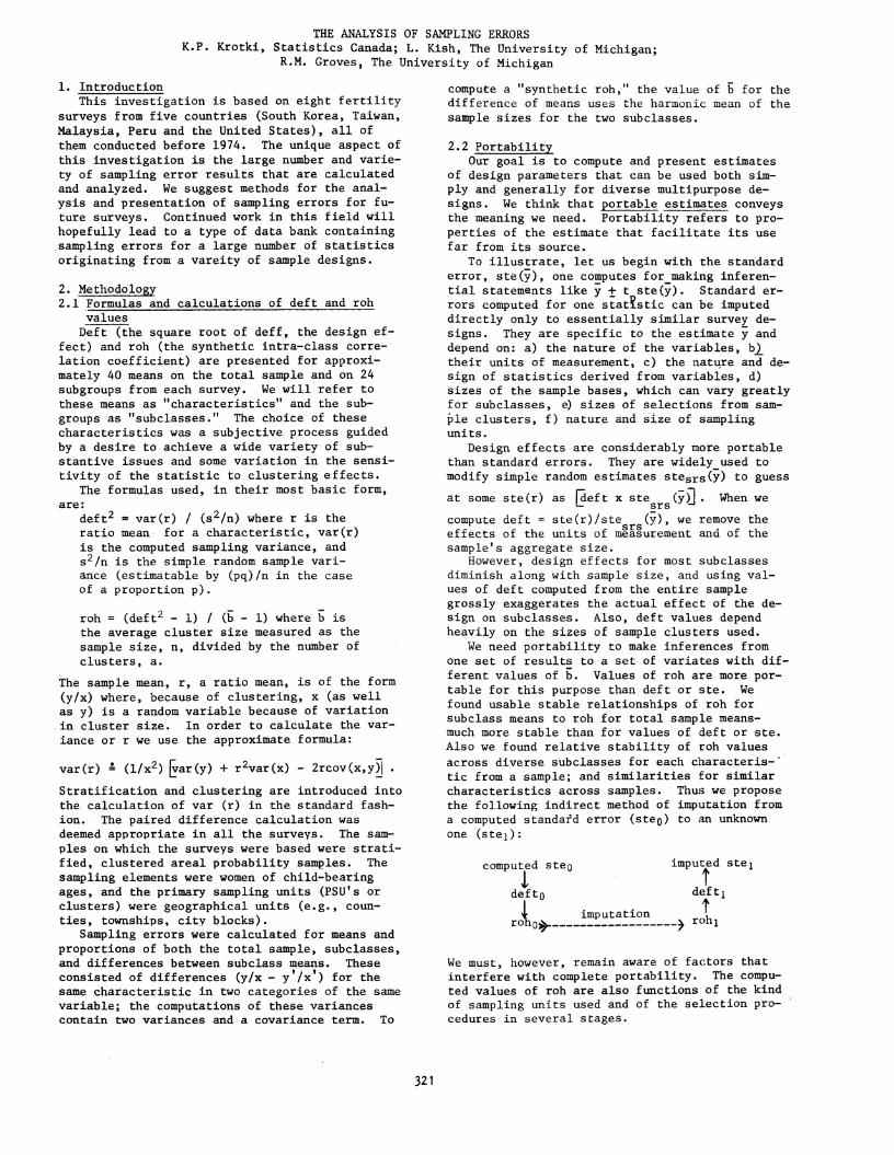
characteristics across samples. Thus we propose
the following indirect method of imputation from a computed standard error (step) to an unknown
one (stet):
computed step imputed stet
defto
imputation
deft).
We must, however, remain aware of factors that
interfere with complete portability. The compu-
ted values of roh are also functions of the kind of sampling units used and of the selection pro-
cedures in several stages.
2.3 The use of roh and deft for imputation We need to impute roh for subclasses from val-
ues computed for the entire sample or for similar type subclasses. Thus we need stability (porta- bility) for roh values and we seem to find that for crossclasses. This type seems to cover most subclasses used in survey analysis. Crossclasses is a term we coined for subclasses that cut a- cross clusters and strata used in the selection process. The sizes of sample clusters for each subclass are roughly b = b M , where M is the
proportion of the subclass insthe samplé and b is for the entire sample. Design effects tend to decrease linearly almost to 1 as the crossclass size decreases and roh remains relatively con- stant. We must first impute some value roh].
rohp from computed values of roh0 and a correc-
tion factor Xi. Then we estimate the unknown deft]. from deft = 1 + X1rohp - 1). We com- puted values of rohp based on means for the en- tire sample for each of 40 characteristics on each survey. We then computed and found values
near (and slightly over) = 1 for the diverse subclasses.
are themselves usually subject to great sampling variability. Many samples are not based on a large enough number of PSU's to yield sufficient precision for individual estimates for sampling errors. In addition, most surveys are highly multipurpose in nature and we must combine re- sults from diverse statistics for joint deci- sions and designs. Some form for combining them must be sought, because combining their re- sults is preferable to its alternatives. We ar- gue against following the common practice of choosing a single variable among many for making inferences about the design and planning future designs.
Several methods were applied to the sampling error results in this investigation in order to identify underlying trends and relationships. Much of what was done was on an ad hoc basis as each survey presented its own idiosyncracies. Thus the methods shown here should be viewed more as a progress report than as final optimal techniques. Hopefully we have pointed out some approaches that may be applicable on a more gen- eral scale.
First, characteristics were listed by order of magnitude of roh. Another approach to arrive at the same information is to group supposedly "similar" characteristics and to calculate the average roh for each group. The mean and range of roh values for the characteristics within each group can serve as summary statistics. Measurements 6n the same characteristics at dif-
ferent points in time or under different survey conditions provide further data on the sampling behavior of these characteristics.
The study of sampling errors for subclasses is an important need because much survey analysis
involves comparisons of subclasses. It is diffi- cult to give guides for how the choice of sub-
classes should be made, but using measures which
are candidates for independent variables in anal- ysis of the data may be desirable. In this view,
the characteristics would be analogous to the de-
322
pendent variables. Comparison of sampling errors for the total sample and for the subclasses can
give the survey designer an idea of how to impute in general from total results to subclasses. This is a common requirement since sampling er- rors cannot be calculated for all possible sub- classes for each characteristic.
3. Empirical Results The above described methodology was applied to
the sampling errors calculated for eight fertili-
ty surveys in five countries. In this section we
discuss in detail the results for one of these
surveys. Detailed analysis of sampling error results
for Taiwan: General Fertility Survey (1973 KAP -4)
3.1 Sample design The universe of 331 townships was divided into
27 strata using level of urbanization, education, and fertility. Within strata, townships were
geographically ordered and 56 were selected sys-
tematically. Within selected townships the sam-
ple had three stages, yielding 5588 married women
aged 20 -39. The coefficient of variation of size
among the 56 ultimate clusters is 0.03 for the
entire sample; within the 24 subclasses used it
ranges from 0:02 to 0.08.
3.2 Results for the total sample Results for 40 characteristics are presented
in Table 1. The characteristics are ordered
from highest to lowest values of roh. Deft val-
ues follow this trend closely with minor excep-
tions due to slight differences in sample bases
(n), hence cluster size (n /a). Note the large
range of roh values (col. 4) for the 40 charac-
teristics, essentially from 0 to 0.3. The quar-
tiles are about 0.075, 0.025 and 0.015. These
correspond to deff values of about 8.4, 3.2, and
Table
Fertility Study (KAP), 1970, Ste'.. Deft's and for 40
Together with Summary Roh Values for and
Char.
1
Mean Std.
Error
3
Total Sample
Deft roh
Sub- Class
6 7
Ave.
rohd
3 Se, preference 5.23 .053 5.41 .290 .334 1.15 .012
2 Currently using contraception 0.45 .010 1.45 .011 .006 0.57 -.002
1 Living sons number 1.54 .021 1.43 .011 .012 1.08 .002
1 Living children number 3.06 .029 1.39 .010 .017 1.75 .0% 1 Pregnant now 0.12 .005 1.21 .005 .005 1.11 -.001 2 Induced abortions number 0.31 .012 1.19 .004 .012 2.72 .004
.0592 .0790 1.436 .00652
Ratios of means col. 5 /col. 4 and col. 7 /col. S 1.334 .083
'The characteristic type denotes: 1) fertility experience. 2) contraceptive practice. 3) birth preferences and desires, 4) attitudes, 5) background, 6) demographic background.
2.5; these large factors arise because of the
large number of elements, almost 100, per cluster.
The mean roh on the total sample is 0.0592. It is useful to observe the clear differences
in roh values between the 6 classes of character-
istics. Attitudinal variables are all in the first quartile, with roh value over 0.075. Birth
preferences and desires are mostly in the top two
quartiles, with roh values over 0.025. Contra-
ceptive practice is spread evenly between the se-
cond quartile (0.075 - 0.025) and the second half
under 0.025. Fertility experience variables are all in the lower half with roh values under 0.025. They are evenly spread among socio- economic (which, in this survey, only indi-
cates literacy) and demographic variables. These three classes of variables (codes 1, 5
and 6) are contained in the lower half, with roh values under 0.025, while classes 3 and 4 are above that.
If roh values were unusually high for all variables, we should look either into causes for unusual segregation in the population or into the choice of small and homogeneous sampling units. However, roh's for demographic variables are not high. Their spread under 0.025 is simi- lar to values found in other populations. Two explanations are possible for the high roh val- ues for the subjective variables of attitides and birth preferences and desires. First, is is sociologically reasonable to think that when at- titudes change rapidly, the spread of the change takes place unevenly and is clustered in areas. Second, clustering of the measured values can be caused by interviewer effects which are not se- parable from the effects of clusters themselves.
3.3 Results for subclasses Clustering of values for subgroups of the sam-
ple was investigated for the 24 subclasses in
Table 2 for each of the 40 characteristics. This
vast amount of data is summarized in Column 5 of
Table 1. Each entry is the mean of the rohs over
the same 24 subclasses of Table 2. This mean
subclass roh is shown as the ratio to the roh for
the total sample (col. 6). Note that the mean
subclass roh values parallel closely the total
roh values. The ratios of sibclass /total roh
values do not vary greatly around their mean of
1.436. A more useful average is .0790/.0592 =
1.334, the ratio of the two mean values. This
gives greater weight to the larger roh's where
more fluctuations can be observed. A quick rule
of thumb woald guide the researcher to use the
total roh times 1.33 to obtain subclass roh's.
This yields
deffsubclass- + 1.33roh Total
(bsubclass -
Column 4 of Table 2 presents values of roh for
each subclass averaged over all 40 characteris-
tics. Column 5 notes the ratios of these aver-
ages to the mean roh value of 0.0592 when the to-
tal sample is the base. For these values of sub-
class bases there exists no clear separation be-
tween socio- economic and demographic subclasses
that we found for them as characteristics. Though the former tend to be a little higher,
most of the variation is within the groups. The
323
Table 2
Taiwan Fertility Study (KAP), 1970, and Rob's for Twenty -four Subclass Variables Treated as Characteristics and Subclass Base.
1 2 3 4 5 6 7
Population Rase Subclass base Differences Ratio
Ave. to Ave. (6)2 Prop. Deft .059i1 (4)
Education Hone .255
of husband Primary .548
Junior High .081 Senior High + .070
Occupation Farmer .219
of husband Labr.40perty. .202
Skilled .149 White Collar + .359
1.684 .0186 .1212 2.05 1.727 .0201 .0615 1.04
1.453. .0112 .0410 0.69
1.739 .0205 .0969 1.64
2.437 .0509 .1474 2.49
2.002 .0310 .0726 1.23
1.951 .0289 .0733 1.24
1.872 .0258 .0525 0.89
Income 0 -23.9 .154 4.171 .1987 .1765 2.98
of family 24. -35.9 .172 1.445 .0132 .0868 1.47
(1000 NT) 35. -47.9 .172 1.807 .0274 .0639 1.08
48. + .303 2.476 .0621 .0671 1.13
Ave. for 12 classes 2.064 .0424 1,494
Children 0 -1
ever born 2
3
4 or more
Marriage duration
.147 1.221 .0050 .0671 1.13
.172 1.122 .0026 .0667 1.13
.239 0.987 -.0002 .0613 1.04
.396 1.429 .0105 .0766 1.29
0 -4 .228 1.139 .0031 .0622 1.05
5 -9 .267 0.874 -.0024 .0647 1.09
10 -19 .386 1.038 .0009 .0741 1.25
20+ .058 1.037 .0008 .0936 1.58
Age 19 -24
of wife 25 -29
30 -34 35 -42
Ave. for 12 classes
.189 1.150 .0032 .0554 0.94
.252 1.187 .0041 .0715 1.21
.260 1.169 .0037 .0678 1.14 ,0006 ,008
.255 0.892 -.0021 .0733 1.24 1.104 1.174 .128
.0101 .111
.0053 .077
.0208 .189
.0041 .065
.0211 .160
.0044 .067
.0110 .112
.0036 .054
.0025 .036
.0031 .049
-.0001 -.001
.0014 .022
Ave. for 24 classes .0790 1.334 .0064 .070
0.0592 is the average roh for the 40 characteristics on the total sample
(see bottom of Col. 4 of Table 1).
In calculating the ratio, the mean of the two entries col. 4 is used.
average roh for the 24 subclasses is 0.0790, and the ratio 0.0790/0.0592 1.334 measures the aver- age increase over the roh value based on the to- tal sample.
3.4 Results for differences between subclass
means We have computed roh values for the difference
of each of 2 pairs in each set of 4 subclasses,
for each of the 40 characteristics. The averages
over the 12 values are shown in col. 7 of Table
1, where rohd is the roh for the difference.
These rohd values are substantially lower than
the corresponding subclass values. The indivi-
dual ratios (not shown) of values in column 6 to
column 4 vary considerably around their average
of .095. A better average is the ratio of means:
.00652/.0790 .083. The individual ratios range
most from 0.30 to 0.00, except from some trivial
cases near the bottom of the table, where nega-
tive values appear. We have also found in many
other studies positive but smaller effects for
differences than for the corresponding subclas-
ses. The effects of covariance between subclas-
ses seem unusually strong in this design. Conse-
quently, the effects of clustering of differences
though still present, are considerably reduced.
In column 6 of Table 2 are shown roh values for
differences of pairs of subclass means. Each of
the 12 entries represents an average over the 40
variables of Table 1. Note the great reductions
in design effects due to positive covariances in
clusters. The ratios of the average rohs is
.0064/.0790 = 0.081.
4. Highlights from other surveys
The 1971 and 1973 South Korea fertility stu-
dies provided an opportunity to study sampling
errors for the same characteristics at two points
in time. At first glance it seemed that the roh
values in 1973 were considerably smaller than
those in 1971. The average roh value for some 40 characteristics was 0.049 in 1971 and 0.033 in 1973. However, when we examined only the subset of characteristics which were common to both sur- veys the average roh values were 0.037 in 1971 and 0.030 in 1973. In this subset the design ef- fects are 3.85 and 2.02 respectively because the average cluster size in 1973 was much smaller than in 1971. This is an example of why we ar- gue for portability in terms of roh rather than deft. The range of roh values in the South Kor- ean fertility surveys was 0 to 0.2.
A fertility survey of Malaysia was conducted in 1969 and yielded 2,950 interviews with women involved in two large family planning programs. The sample was drawn after stratification into rural and urban areas. It was found that the de- sign effects were far larger in the rural than in the urban areas. For 29 variables, the average deft's for the rural and urban areas were 1.92 and 0.99 respectively. The average roh for rural areas was 0,046. In the urban areas there was no clustering since the respondents were selected individually from lists of names. The range
of roh values for the total sample was 0.02 to 0.05.
Arranging the characteristics by size of roh revealed two striking results. The characteris- tics "proportion using NFPB clinic," "proportion Malay" and "proportion with farmer husband" pro- duced abnormally large sampling errors (deft's of 4.06, 2.65 and 2.58 and roh's of 0.36, 0.14 and 0.13 respectively). The first is explained by the fact that women in a given cluster either attended one type of clinic or the other. (This variable could have been an appropriate strati- fication variable.) The second result suggests that ethnicity is a highly clustered variable in Malaysia. The third result is due to the fact that clusters follow geographical boundaries with diverse densities of farmers.
Another result gleaned form the Malaysia sur- vey is that subclasses that approximate crossclasses produce different sampling errors than do subclasses that are segregation classes. Over 5 pairs of crossclasses (e.g., income, age, marital status) the average roh across 14 char- acteristics was 0.0318, which has a ratio of 1.15 to the average roh for these characteristics on the total sample. On the other hand, if we con- sider the segregation classes (e.g., type of cli- nic, ethnicity, rural -urban birth and farmer -non- farmer occupation) the average roh is 0.0750.
5. Summary of Results from Eight Surveys For each survey sampling errors were computed
for about 30 to 40 characteristics. This was done in each survey for means based on the entire sample and on about 24 subclasses and for differ- ences between about 12 pairs of subclass means.
The great range across different variables in
values of roh in each of the surveys is the most important result. The roh values have an effec- tive hundredfold range in each survey from about 0.001 to 0.002 to about 0.1 or 0.2.
Some differences between types of variables can be detected on each survey in Table 3. How- ever these differences are not consistent and are also marked by considerable sampling variability. Socio- economic variables appear noticeably high
324
for Korea and Peru. Demographic background var- iables tend to be near the lower end for all sur- veys. Attitudes and birth preferences appear high though more often in the lower half with roh values mostly from 0.005 to 0.05. The ranges within types (not shown) seem to be factors of a- bout 5 to 10. They are considerably less than the range of 50 or 100 for rohs of all variables within surveys. Thus the typing of variables seems an effective and simple way to reduce our
level of ignorance.
The individual computations of rohs for each
characteristic /subclass combination are subject
to great variability. But the average roh for
each characteristic computed over several sub- classes is quite stable. We refer to subclasses that are approximately crossclasses (more or
less evenly distributed in the sample clusters). Other kinds of subclasses, those that are very unevenly distributed in sample clusters, need special considerations.
Table 3 summarizes a vast body of computa- tions over the eight surveys. Since the varia- bles included had not been coordinated initially, it is comforting that some very useful stabili- ties may nevertheless be drawn from them. The average values of overall rohs (first row) var- ies from .024 to .063. This stability is quite
good, considering the diversity of variables and sample designs. It is helpful for choice of sample designs, since accepting .04 or .05 for
roh would not badly mislead one. For fertility experience and demographic background variables, the roh values are lower and more stable, .011
to .038. For general attitudinal variables the roh values are very high for Taiwan and Peru and fertility preferences are also high in Taiwan. It would be interesting to investigate how much
TABLE 3
Rohs for Survey.
STATISTIC
SAMPLE SURVEY
South Korea Taiwan Peru Malaysia United States
1971 1973 1960 1970 White,
A. ROB'S FOR TYPES OF VARIABLES FOR TOTAL SAMPLE (Number of characteristic. below
1. All Characteristics .050 .033 .059 .063 .045 .024 .037
The eighth vey perteloing to blacks In 1970 unreliable due to design sad moll
b high for unknown
for cro.tcla.aes only.
4 result breed oa Bubo). one of tae. ratio te 1.1s.
of these high roh values are due to homogeneity of the respondents in compact clusters, or how much of the effects of interviewer variance of response from large workloads. The high roh values for socio- economic variables in Peru and South Korea have implications for sample designs, as well as for sociological studies of their sources.
When we separate socio- economic subclasses from others we regularly note considerable dif-
ferences between the two groups, when these are computed as characteristics based on the entire sample (rows 13 and 14). However, when used as subclasses (rows 15 and 16) the differences'be- tween the two sets of 'subclass roh's (averaged over all characteristics) are not great, say 1.2 versus 1.4. It is the characteristics, much more than the subclass, that are the sources of variability in sampling errors.
The ratio of the rohd's for difference to the
average roh's for subclass means (rows 11 and 12) is not stable. In all cases the reductions due to covariances between clusters are substantial. The central value may be 0.1 and 0.2.
6. Strategies for Large -Scale Calculation, Sum-
marization and Presentation of Sampling Errors (1) Paired selection considerably simplifies
sampling error calculations. (2) The coefficient of variation of cluster
size should always be calculated and in-
spected before the results of sampling error calculations are published, since
the approximate formula for var(r) re-
quires cv(x) <0.2.
(3) Codes identifying the primary sampling units and the strata must be included together with the data. Our experience has been that these codes are seldom readily available.
(4) Sampling errors should be calculated for the entire sample for many variables. We
think it inadequate to single out a few critical survey variables or several cate- gories of one variable. Rather than ex- hausting all categories for a few varia- bles, more variables should be used, each one for one or a few categories. Variabi-
lity between variables is generally great- er than between categories within varia- bles. This is especially true for char- acteristics, but also for subclass vari- ables. The range of variables should parallel the aims of the survey, of its
analysts and of its users. Also, it
should aim to cover the range of design effects.
(5) The variables should be separated into a
few groups within which the sampling er- rors are expected to be relatively simi-
lar.
(6) Sampling errors should be computed for many characteristics each based on a mode- rate number of subclasses. Sampling er- rors, particularly roh's, were found sub-
ject to greater diversity across charac-
teristics than across subclasses. Sub-
class results should be compared to the results obtained for the total sample.
325
(7) Most of the needed subclasses tend to ap- proximate crossclasses. However, partial- ly segregated subclasses, if important, should also be investigated.
(8) In choosing subclass categories a range of subclass sizes should be selected to ob- tain empirical evidence of the effect of subclass size on deft and roh.
(9) All chosen characteristics should be anal- yzed by all chosen subclasses (rather than using different subclasses for each char- acteristics). This yields a symmetrical table and averaging can be done over both subclasses and characteristics. However, other designs may be used, especially for a larger number of subclasses.
(10) Sampling errors should be computed for the difference of means of pairs of subclass- es. For many subclass variables one or two pairs usually suffice. These results
should be compared with the individual re- sults for each of the two subclasses.
(11) Sampling error results should be preserved and publicized for the use of survey de signers who would find such data useful in the design of future surveys.
In addition to the 40 characteristics that we treated as "dependent," we also computed roh val- ues for 24 variables later used for subclass an- alysis. Here a clear dichotomy emerged. The 12 characteristics based on demographic variables had roh values under 0.005 (Table 2, col. 3).
However, the 12 socioeconomic characteristics had roh values 0.01 to 0.20. Within the two classes of characteristics there is variation, but much of it is too haphazard to be of general use.