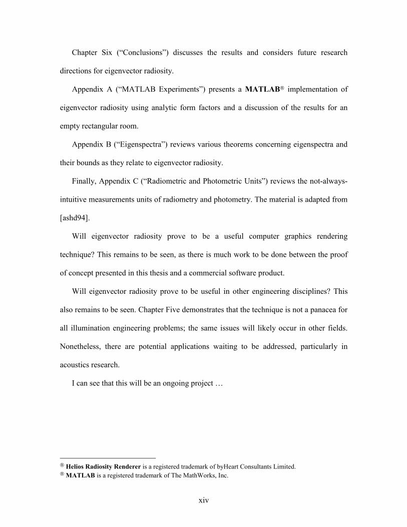
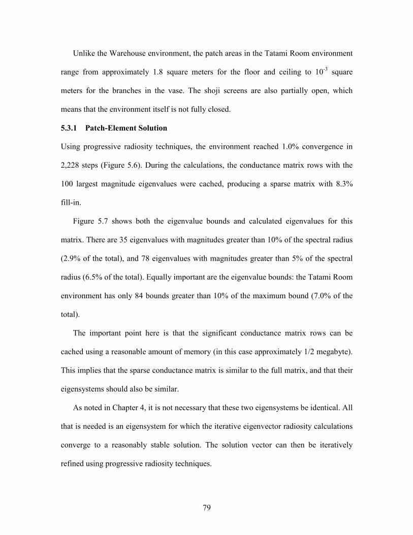
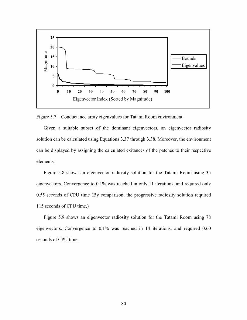
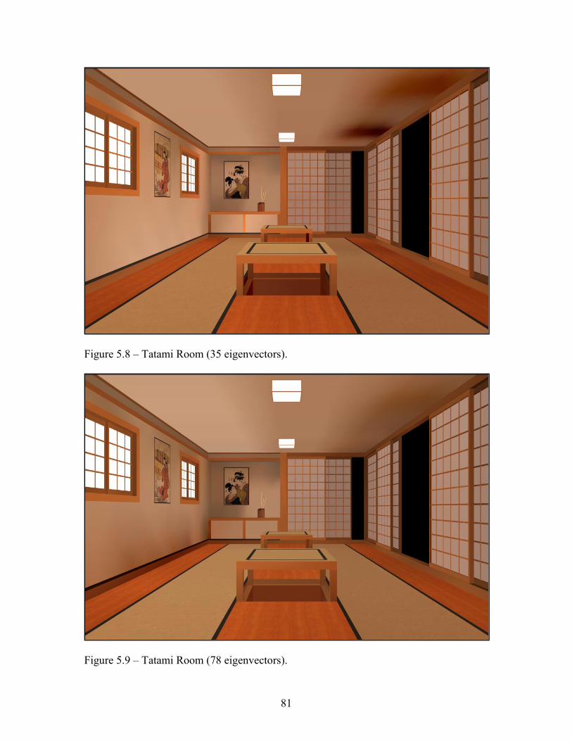
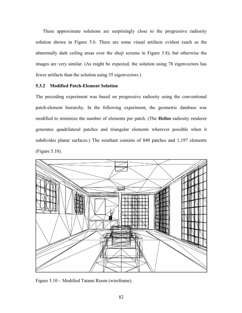
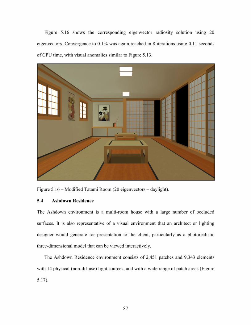
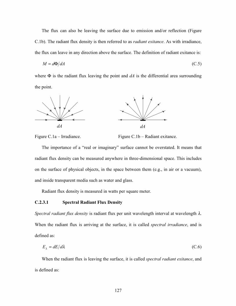
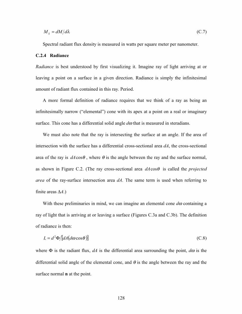
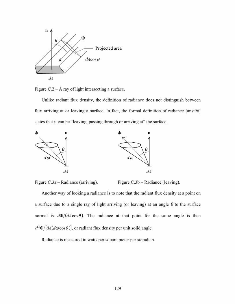
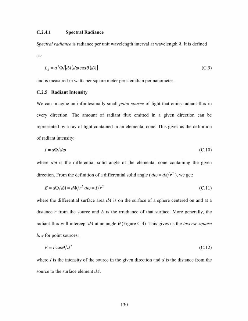
Engineers may not require photorealistic image synthesis, but they will demand
calculation tools that are as fast as possible. Unfortunately, the radiosity method is
compute-intensive.
An architectural lighting design visualization (e.g., Figure 1.1) may require several
minutes of calculation time on a desktop personal computer. While this is in itself
4
reasonable, it is only a small portion of the design process. On viewing the associated
isolux plots, the lighting designer may choose to change or reposition the luminaires.
Similarly, the architect or client may request changes to the wall finishes and floor
coverings.
It is therefore desirable to have the ability to quickly recalculate the luminous flux
distribution within an architectural environment when such design changes are made.
Ideally the calculations should take seconds rather than minutes – this would provide
lighting designer and architects with a truly interactive engineering design tool.
The benefits of such a design tool would not be limited to lighting designers and
illumination engineering. As another example, aerospace engineers need to analyze the
solar heating characteristics of satellites. Because the distribution of solar radiant flux
changes as the satellite rotates, radiosity calculations must be performed for dozens to
hundreds of different orientations. Any improvement in the calculation times would be
welcome.
Acoustical engineers would also benefit from an interactive acoustic radiosity design
tool. Ideally, this tool would allow for real-time playback of arbitrary sound sources
where both the source and the listener are moving through the environment.
The goal of this thesis is to develop a radiosity method that will meet these
requirements.
1.2 Radiosity Explained
The underlying principles of radiosity are most easily explained with an example.
Consider the rectangular room shown in Figure 1.2. It has a luminaire mounted on the
5
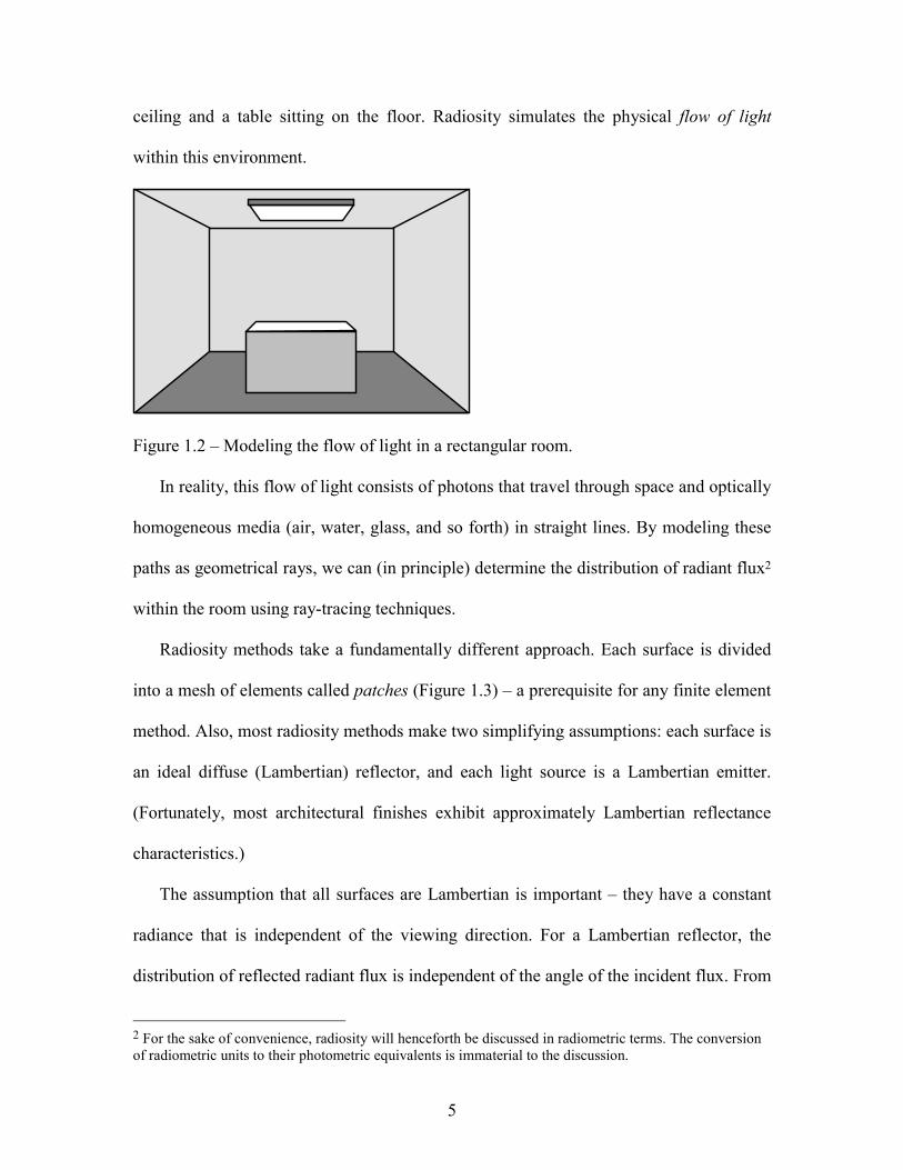
ceiling and a table sitting on the floor. Radiosity simulates the physical flow of light
within this environment.
Figure 1.2 – Modeling the flow of light in a rectangular room.
In reality, this flow of light consists of photons that travel through space and optically
homogeneous media (air, water, glass, and so forth) in straight lines. By modeling these
paths as geometrical rays, we can (in principle) determine the distribution of radiant flux2
within the room using ray-tracing techniques.
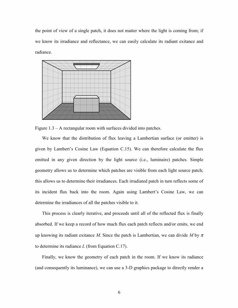
Radiosity methods take a fundamentally different approach. Each surface is divided
into a mesh of elements called patches (Figure 1.3) – a prerequisite for any finite element
method. Also, most radiosity methods make two simplifying assumptions: each surface is
an ideal diffuse (Lambertian) reflector, and each light source is a Lambertian emitter.
(Fortunately, most architectural finishes exhibit approximately Lambertian reflectance
characteristics.)
The assumption that all surfaces are Lambertian is important – they have a constant
radiance that is independent of the viewing direction. For a Lambertian reflector, the
distribution of reflected radiant flux is independent of the angle of the incident flux. From
2 For the sake of convenience, radiosity will henceforth be discussed in radiometric terms. The conversion of radiometric units to their photometric equivalents is immaterial to the discussion.
6
the point of view of a single patch, it does not matter where the light is coming from; if
we know its irradiance and reflectance, we can easily calculate its radiant exitance and
radiance.
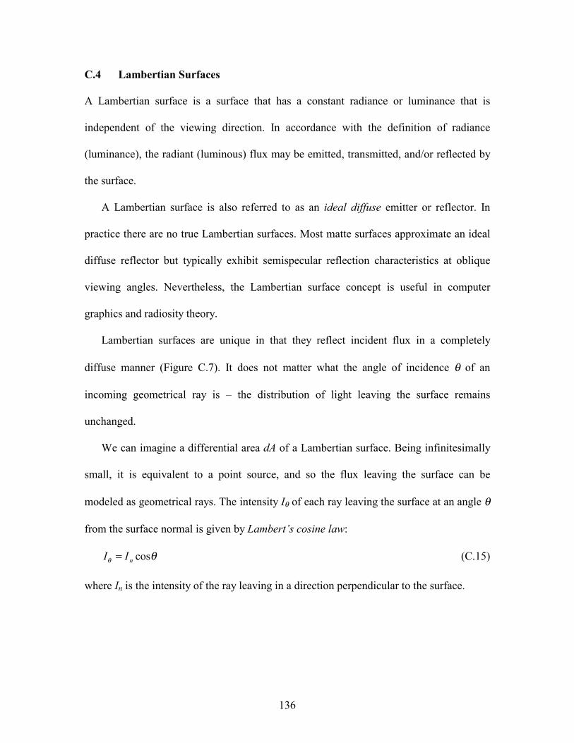
Figure 1.3 – A rectangular room with surfaces divided into patches.
We know that the distribution of flux leaving a Lambertian surface (or emitter) is
given by Lambert’s Cosine Law (Equation C.15). We can therefore calculate the flux
emitted in any given direction by the light source (i.e., luminaire) patches. Simple
geometry allows us to determine which patches are visible from each light source patch;
this allows us to determine their irradiances. Each irradiated patch in turn reflects some of
its incident flux back into the room. Again using Lambert’s Cosine Law, we can
determine the irradiances of all the patches visible to it.
This process is clearly iterative, and proceeds until all of the reflected flux is finally
absorbed. If we keep a record of how much flux each patch reflects and/or emits, we end
up knowing its radiant exitance M. Since the patch is Lambertian, we can divide M by π
to determine its radiance L (from Equation C.17).
Finally, we know the geometry of each patch in the room. If we know its radiance
(and consequently its luminance), we can use a 3-D graphics package to directly render a
7
photorealistic image of the room as a collection of shaded 3-D polygons from any
viewpoint.
1.3 Form Factors
The most difficult aspect of developing a radiosity rendering program has nothing
whatsoever to do with light per se. The claim in Section 1.2 that “simple geometry allows
us to determine which patches are visible from each patch” is true, but only in an intuitive
sense. Solving this problem analytically is anything but simple!
Stated in more formal terms, the problem is this: knowing the radiant exitance of one
Lambertian patch, what portion of its flux will be received by a second patch in an
environment?
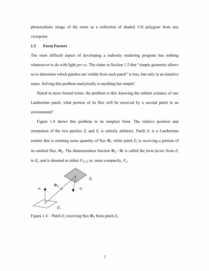
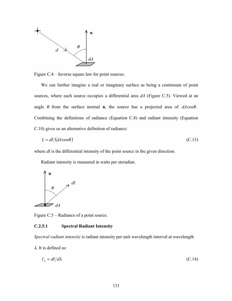
Figure 1.4 shows this problem in its simplest form. The relative position and
orientation of the two patches Ei and Ej is entirely arbitrary. Patch Ei is a Lambertian
emitter that is emitting some quantity of flux Φi, while patch Ej is receiving a portion of
its emitted flux, Φij. The dimensionless fraction Φij / Φi is called the form factor from Ei
to Ej, and is denoted as either FEi-Ej or, more compactly, Fij.
Figure 1.4 – Patch Ej receiving flux Φij from patch Ei.
nj ni Φij
Ej
Ei
8
The problem is deceptively simple. The total flux emitted by patch Ei is Φi = MiAi,
where Mi is its radiant exitance and Ai is its area. The flux received by Ej is Φij = FijΦi.
Unfortunately, calculating Fij can be an extremely difficult problem in analytic geometry.
1.3.1 Form Factor Geometry
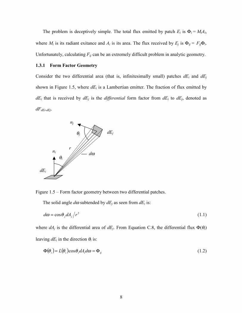
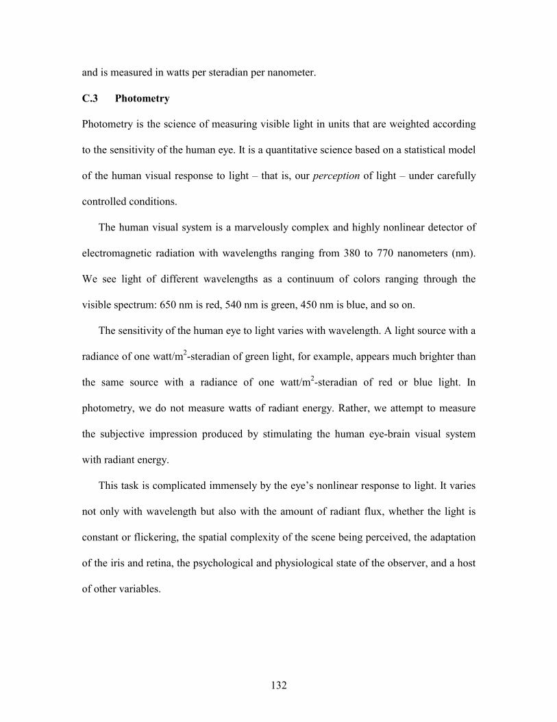
Consider the two differential area (that is, infinitesimally small) patches dEi and dEj
shown in Figure 1.5, where dEi is a Lambertian emitter. The fraction of flux emitted by
dEi that is received by dEj is the differential form factor from dEi to dEj, denoted as
dFdEi-dEj.
Figure 1.5 – Form factor geometry between two differential patches.
The solid angle dω subtended by dEj as seen from dEi is:
2cos rdAd jjθω = (1.1)
where dAj is the differential area of dEj. From Equation C.8, the differential flux Φ(θi)
leaving dEi in the direction θi is:
( ) ( ) ijiiii ddAL Φ==Φ ωθθθ cos (1.2)
dEj
dEi
ni
nj
dω θi
θj
r
9
where L(θi) is the radiance of dEi in the direction θi. Since dEi is a Lambertian emitter,
L(θi) = Li (a constant) for all directions θi. Substituting this and Equation 1.1 for dω
gives:
2coscos rdAdAL jijiiij θθ=Φ (1.3)
Since dEi is a Lambertian emitter, the total emitted flux Φi is given by Equation C.17,
or:
iiiii dALdAM π==Φ (1.4)
The form factor dFdEi-dEj for two differential area patches is thus:
22 coscos
coscosrdA
rdALdAdAL
dF jjiii
jijiidEjdEi πθθ
πθθ
==− (1.5)
Now, suppose that dEj is the Lambertian emitter and dEi is receiving its flux, namely
Φji. We can determine the reciprocal differential form factor dFdEj-dEi by simply reversing
the patch subscripts in Equation 1.5. Doing so illustrates the reciprocity relation for form
factors between any two differential areas dEi and dEj:
dEidEjjdEjdEii dFdAdFdA −− = (1.6)
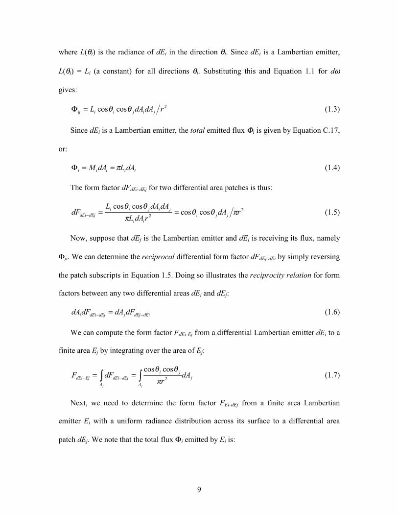
We can compute the form factor FdEi-Ej from a differential Lambertian emitter dEi to a
finite area Ej by integrating over the area of Ej:
jA
ji
AdEjdEiEjdEi dA
rdFF
jj
∫∫ == −− 2
coscosπ
θθ (1.7)
Next, we need to determine the form factor FEi-dEj from a finite area Lambertian
emitter Ei with a uniform radiance distribution across its surface to a differential area
patch dEj. We note that the total flux Φi emitted by Ei is:
10
iii AM=Φ (1.8)
while the flux Φij received by dEj is:
iA
dEjdEiiij dAdFMi
∫ −=Φ (1.9)
(Note that we are now integrating over the area of Ei rather than Ej.)
Figure 1.6 – Determining the form factor FdEi-Ej by area integration over Ej.
From our definition of a form factor, we then have:
∫∫
−
−
− ==ΦΦ
=i
i
AidEjdEi
iii
AidEjdEii
i
ijdEjEi dAdF
AAM
dAdFMF 1 (1.10)
which yields:
iA
ji
i
jdEjEi dA
rAdA
Fi
∫=− 2
coscosπ
θθ (1.11)
Of course, our interest is in patch-to-patch form factors, or the form factor from a
finite area Ei to another finite area Ej. For this, we need to integrate over the areas of Ei
and Ej. (In physical terms, we need to consider the contribution of each differential area
of Ei to the illuminance of Ej). The flux received by Ej is then:
iA
EjdEiiij dAFMi
∫ −=Φ (1.12)
dEjn
Ej
dEi
11
so that the form factor FEi-Ej is:
∫∫
−
−
− ==i
i
AiEjdEi
iii
AiEjdEii
EjEi dAFAAM
dAFMF 1 (1.13)
From Equation 1.7, this yields the double area integral equation:
ijA A
ji
iEjEi dAdA
rAF
i j
∫ ∫=− 2
coscos1π
θθ (1.14)
The reciprocal form factor FEj-Ei is obtained by reversing the patch subscripts. This
demonstrates that the reciprocity relation (Equation 1.6) also holds true for finite area
patches. In other words:
jijiji FAFA = (1.15)
The importance of the reciprocity relation cannot be overstated. It says that if we can
somehow calculate the form factor Fij from an patch Ei to another patch Ej, then we can
trivially calculate the reciprocal form factor Fji. This is a key concept in radiosity theory.
The above equations implicitly assume that the two patches Ei and Ej are fully visible
to each other. In a complex environment, two patches may be partially hidden by one or
more occluding objects. If so, then a suitable term must be added to account for the
occlusions, such as:
ijijA A
ji
iEjEi dAdAHID
rAF
i j
∫ ∫=− 2
coscos1π
θθ (1.16)
where the term HIDij accounts for the possible occlusion of each point of patch Ej as seen
from each point of patch Ei.
12
There are unfortunately no practical analytical methods for solving this equation; it
must typically be solved using numerical quadrature or Monte Carlo ray tracing methods
[e.g., cohe93].
1.3.2 Form Factor Properties
A form factor is a dimensionless constant representing the fraction of flux emitted by one
surface patch that is received by another. It takes into account the shape and relative
orientation of both surfaces and the presence of any obstructions, but is otherwise
independent of any surface properties.
Form factors were first developed for use in thermal and illumination engineering,
where they have been variously called shape, configuration, and angle and view factors.
The thermal engineering literature is filled with discussions of form factor algebra, of
which the reciprocity relation is only one example. Most of these discussions relate to a
time when form factors were calculated by hand. Some properties, however, are still
useful. For example, the summation relation states that:
11
=∑=
n
jijF (1.17)
for any patch Ei in a closed environment with n patches. (A closed environment is one
where all of the flux emitted by any one patch must be received by one or more patches
in the environment. In other words, none of it can escape into free space.) This
summation includes the form factor Fii, which is defined as the fraction of flux emitted by
Ei that is also directly received by Ei. Clearly, Fii can only be nonzero if Ei is concave.
Thus:
0=iiF if Ei is planar (i.e., flat) or convex, and
13
0≠iiF if Ei is concave
Most radiosity methods model surface patches as planar polygons, so that Fii is
always zero.
1.4 The Radiosity Equation
If patches Ei and Ej are both Lambertian surfaces, the form factor Fij indicates the fraction
of flux emitted by Ei that is received by Ej. Similarly, the reciprocal form factor Fji
indicates the fraction of flux emitted by Ej that is received by Ei. However, form factors
in themselves do not consider the flux that is subsequently reflected from these receiving
patches.
Remember that we are trying to determine the radiant exitance Mi of each patch Ei in
an n-patch environment. This exitance is clearly due to the flux initially emitted by the
patch plus that reflected by it. The reflected flux comes from all of the other patches Ej
visible to Ei in the environment.
Consider any patch Ej that is fully visible to Ei. The flux leaving patch Ej is Φj = MjAj.
The fraction of this flux received by patch Ei is Φji = MjAjFji. Of this, the flux
subsequently reflected by Ei is ρiMjAjFji, where ρi is the reflectance of Ei. This gives us:
ijijjiij AFAMM ρ= (1.18)
where Mij is defined as the exitance of Ei due to the flux received from Ej. Using the
reciprocity relation, we can rewrite this as:
ijjiij FMM ρ= (1.19)
To calculate the final exitance Mi of patch Ei, we must consider the flux received by
Ei from all other patches Ej. Thus:
14
ij
n
jjioii FMMM ∑
=
+=1
ρ (1.20)
where Moi is the initial exitance of patch Ei due to its emitted flux only. Rearranging
terms results in:
∑=
−=n
jijjiioi FMMM
1
ρ (1.21)
We can express this equation for all the patches E1 through En as a set of n
simultaneous linear equations:
( )( )
( )nnnnnnnnnn
nn
nnn
FMFMFMMM
FMFMFMMMFMFMFMMM
ρρρ
ρρρρρρ
+++−=
+++−=+++−=
K
K
K
K
22110
2222222112202
112211111101
(1.22)
which we can write in matrix form as:
−−−
−−−−−−
=
nnnnnnnn
n
n
on
o
o
M
MM
FFF
FFFFFF
M
MM
K
K
KKKK
K
K
K
2
1
21
22222212
11121111
2
1
1
11
ρρρ
ρρρρρρ
(1.23)
In matrix notation, this can be succinctly expressed as:
( )MTIM −=o (1.24)
where I is the n × n identity matrix, M is the final n × 1 exitance vector, Mo is the initial
n × 1 exitance vector, and T is an n × n matrix whose (i,j)th element is ρiFij. The matrix
( )TI − is called the radiosity matrix.
This is the elegantly simple radiosity equation: a set of simultaneous linear equations
involving only surface reflectances, patch form factors, and patch exitances. Solving
15
these equations provides us with the radiant exitance, radiance, and ultimately luminance
of every patch in the environment it describes3.
Given a set of initial patch exitances Moi, we need to solve the radiosity equation for
the final patch exitances Mi. The matrix order is typically too large for direct methods
such as Gaussian elimination. However, the radiosity equation is ideally suited for
iterative techniques such as the Jacobi and Gauss-Seidel methods [e.g., golu96]. These
methods are guaranteed to converge to a solution, because the matrix is always strictly
diagonally dominant for flat and convex patches. That is, ρiFij is always less than one,
while Fii is always zero. Furthermore, they converge very quickly, typically in six to eight
iterations [cohe86]. We will examine these methods and a more powerful and useful
variation called Southwell iteration (also known as “progressive radiosity”) in the next
chapter.
3 Solving the radiosity equation for an environment is equivalent to determining its “energy balance.”
The amount of radiant flux reflected and absorbed by a patch must equal the amount of flux incident on its
surface. Flux is energy per unit time. If this balance is not maintained, the patch will steadily accumulate or
lose energy over time. The final solution to the radiosity equation therefore ensures that the flow of energy
is balanced for all patches in the environment.
16
Chapter 2
Solving the Radiosity Equation
2.1 Full Radiosity
We saw in Chapter One that the radiosity equation is a system of n linear equations of the
form:
−−−
−−−−−
=
nnnnnnnn
n
on
o
o
M
MM
FFF
FFFFF
M
MM
K
K
KKKK
KK
K
K2
1
21
222212
11121111
2
1
1
11
ρρρ
ρρρρρ
(2.1)
where n is the number of surface patches in the environment. We know the initial
exitance vector; its entries Moi will be mostly zeroes. The only non-zero entries are for
those patches representing Lambertian light sources. We also know the reflectivity ρi of
each patch, and we can estimate the form factor Fij between any two patches i and j. All
we have to do to obtain the final exitances Mi is to solve these equations.
Most environments result in linear systems that are far too large to solve using direct
methods such as Gaussian elimination. The classic alternative is to use iterative
techniques such as the Gauss-Seidel method [e.g. golu96]. This was the original approach
taken by Goral et al. [gora84]. Baum et al. [baum89] referred to it as the full radiosity
algorithm.
Unfortunately, this gives us a radiosity algorithm with O(n2) time and space
complexity. Even a moderately complex environment with 50,000 patches can easily
17
consume one to ten gigabytes of memory for its form factors and take days of CPU time
to compute a single image. We clearly need a better approach.
What we really want is an algorithm that consumes a minimal amount of memory and
that generates a reasonable approximation of the final image almost immediately. More
generally, we need to maintain a careful balance between the requirement for
photorealistic images and the demands of interactive computing.
In a perfect world, our algorithm would generate a reasonable first approximation
(that can be displayed as a bitmap image) and then progressively and gracefully refine the
solution until it reaches its final form. This essentially describes how iterative techniques
work, except that we need a much more effective algorithm than the Gauss-Seidel
method.
The great surprise is that such an algorithm actually exists. Before examining it,
however, we should review the basic principles of iterative techniques.
2.2 Iterative Techniques
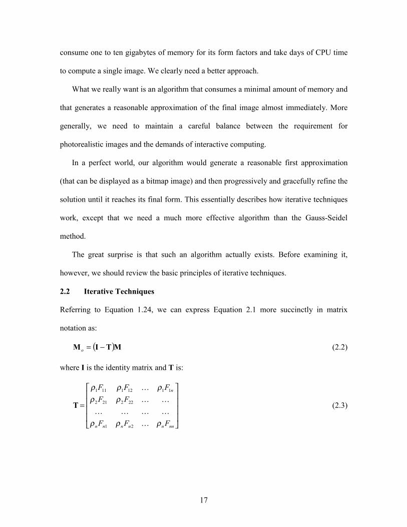
Referring to Equation 1.24, we can express Equation 2.1 more succinctly in matrix
notation as:
( )MTIM −=o (2.2)
where I is the identity matrix and T is:
=
nnnnnnn
n
FFF
FFFFF
ρρρ
ρρρρρ
K
KKKK
KK
K
21
222212
11121111
T (2.3)
18
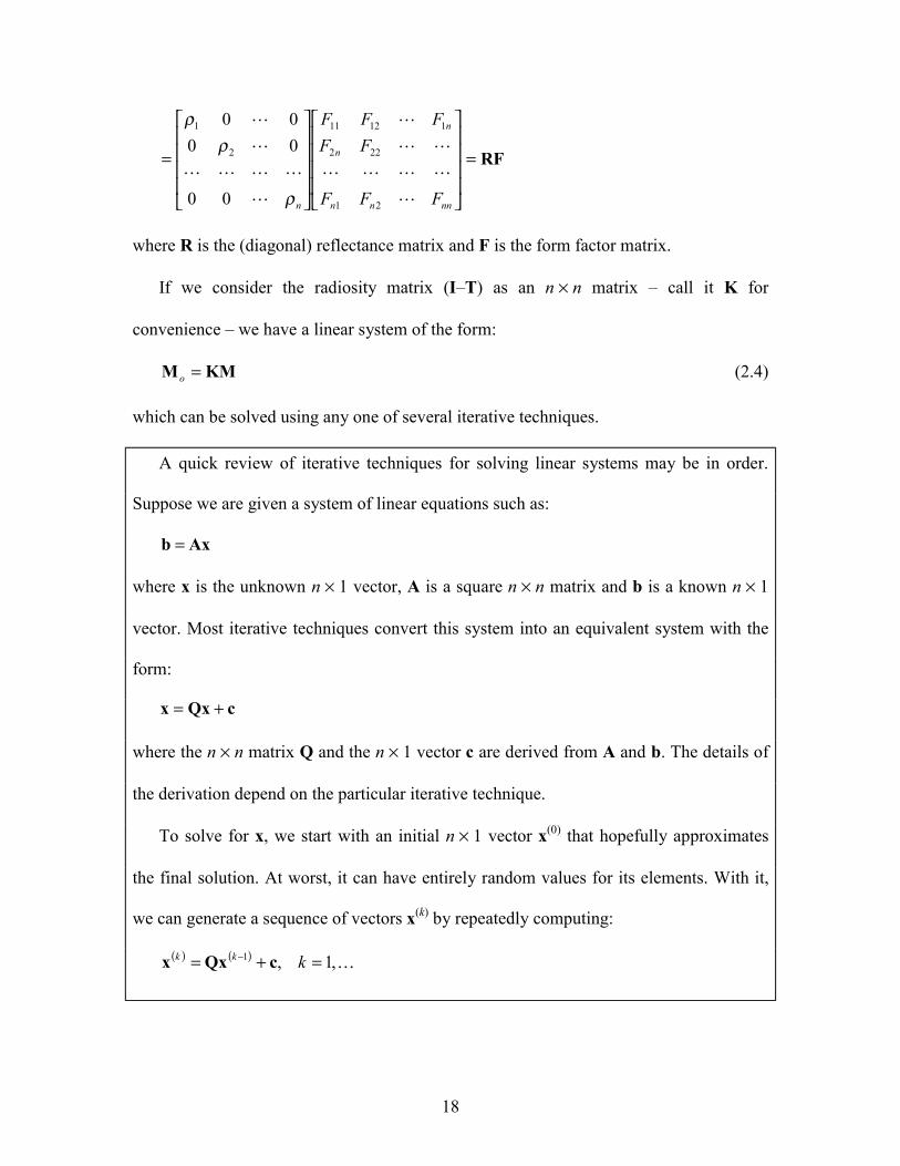
RF=
=
nnnn
n
n
n FFF
FFFFF
L
LLLL
LL
L
L
LLLL
L
L
21
222
11211
2
1
00
0000
ρ
ρρ
where R is the (diagonal) reflectance matrix and F is the form factor matrix.
If we consider the radiosity matrix (I–T) as an n × n matrix – call it K for
convenience – we have a linear system of the form:
KMM =o (2.4)
which can be solved using any one of several iterative techniques.
A quick review of iterative techniques for solving linear systems may be in order.
Suppose we are given a system of linear equations such as:
Axb =
where x is the unknown n × 1 vector, A is a square n × n matrix and b is a known n × 1
vector. Most iterative techniques convert this system into an equivalent system with the
form:
x Qx c= +
where the n × n matrix Q and the n × 1 vector c are derived from A and b. The details of
the derivation depend on the particular iterative technique.
To solve for x, we start with an initial n × 1 vector x(0) that hopefully approximates
the final solution. At worst, it can have entirely random values for its elements. With it,
we can generate a sequence of vectors x(k) by repeatedly computing:
( ) ( ) K,1,1 =+= − kkk cQxx
19
This is the iterative component of the technique. The sequence of vectors x(k) will be
such that the elements of the vector either converge to those of the unknown vector x, or
else diverge into some random vector, as k increases.
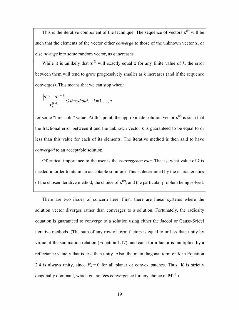
While it is unlikely that x(k) will exactly equal x for any finite value of k, the error
between them will tend to grow progressively smaller as k increases (and if the sequence
converges). This means that we can stop when:
( ) ( )
( ) nithresholdk
i
ki
ki ,,1,
1
1
K=≤−
−
−
x
xx
for some “threshold” value. At this point, the approximate solution vector x(k) is such that
the fractional error between it and the unknown vector x is guaranteed to be equal to or
less than this value for each of its elements. The iterative method is then said to have
converged to an acceptable solution.
Of critical importance to the user is the convergence rate. That is, what value of k is
needed in order to attain an acceptable solution? This is determined by the characteristics
of the chosen iterative method, the choice of x(0), and the particular problem being solved.
There are two issues of concern here. First, there are linear systems where the
solution vector diverges rather than converges to a solution. Fortunately, the radiosity
equation is guaranteed to converge to a solution using either the Jacobi or Gauss-Seidel
iterative methods. (The sum of any row of form factors is equal to or less than unity by
virtue of the summation relation (Equation 1.17), and each form factor is multiplied by a
reflectance value ρ that is less than unity. Also, the main diagonal term of K in Equation
2.4 is always unity, since Fii = 0 for all planar or convex patches. Thus, K is strictly
diagonally dominant, which guarantees convergence for any choice of M(0).)
20
Second, we need to consider what our choice of M(0) should be. The closer it is to the
unknown final exitance vector M, the more quickly our chosen iterative method will
converge. Of course, the only a priori information we have concerns the initial exitances
of the patches representing Lambertian light sources1. In other words, our best choice is
to assign the initial exitance vector Mo to M(0). Interestingly enough, this choice has some
physical significance.
2.2.1 Follow the Bouncing ………… Light
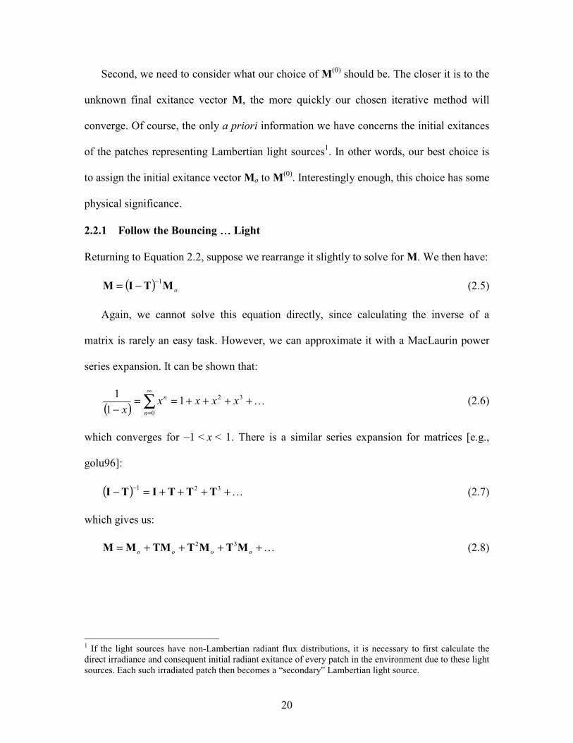
Returning to Equation 2.2, suppose we rearrange it slightly to solve for M. We then have:
( ) oMTIM 1−−= (2.5)
Again, we cannot solve this equation directly, since calculating the inverse of a
matrix is rarely an easy task. However, we can approximate it with a MacLaurin power
series expansion. It can be shown that:
( ) K++++==− ∑
∞
=
32
0
11
1 xxxxx n
n (2.6)
which converges for –1 < x < 1. There is a similar series expansion for matrices [e.g.,
golu96]:
( ) K++++=− − 321 TTTITI (2.7)
which gives us:
K++++= oooo MTMTTMMM 32 (2.8)
1 If the light sources have non-Lambertian radiant flux distributions, it is necessary to first calculate the direct irradiance and consequent initial radiant exitance of every patch in the environment due to these light sources. Each such irradiated patch then becomes a “secondary” Lambertian light source.
21
that converges if the spectral radius of T (i.e., the absolute value of its largest eigenvalue)
is less than one. Fortunately, this condition is true for any physically possible radiosity
equation [e.g., heck91].
There is an important physical significance to Equation 2.8 [e.g., kaji86]. Each
successive term TkM represents the kth bounce of the initially emitted light. The term Mo
represents the initial flux (i.e., the direct illumination), TMo represents the first bounce
component, T2Mo the second bounce and so on. We can intuitively see this by observing
that the patch reflectances ρ are multiplied with each successive bounce. This represents
the accumulating light losses due to absorption.
We can express Equation 2.8 in its iterative form as:
( ) ( ) 0,1 >+= − kokk MTMM (2.9)
In other words, the behavior of light flowing through an environment is itself an iterative
method. Moreover, the initial exitance vector Mo serves as its initial estimate to the final
exitance vector M.
Comparing Equation 2.9 to iterative techniques for solving linear systems, it becomes
clear why the radiosity equation always converges to a solution when we apply these
techniques. To do otherwise – that is, for the approximate solution vector M(k) to diverge
with increasing values of k – would require the total quantity of light in an environment
to increase with each successive bounce. This would in turn contravene the energy
balance discussed in Section 1.4.
There is in fact only one iterative technique that faithfully models the physical reality
of light’s behavior as expressed by Equation 2.9. It is the Jacobi iterative method, the
simplest iterative technique for solving systems of linear equations. While it may not be
22
necessary for our development of a practical algorithm for solving the radiosity equation,
we should ask how the Jacobi method works for two reasons.. First, it will provide us
with a better understanding of how and why iterative techniques work. More important,
however, the Jacobi method offers a fascinating and instructive insight into the physical
reality of the radiosity equation.
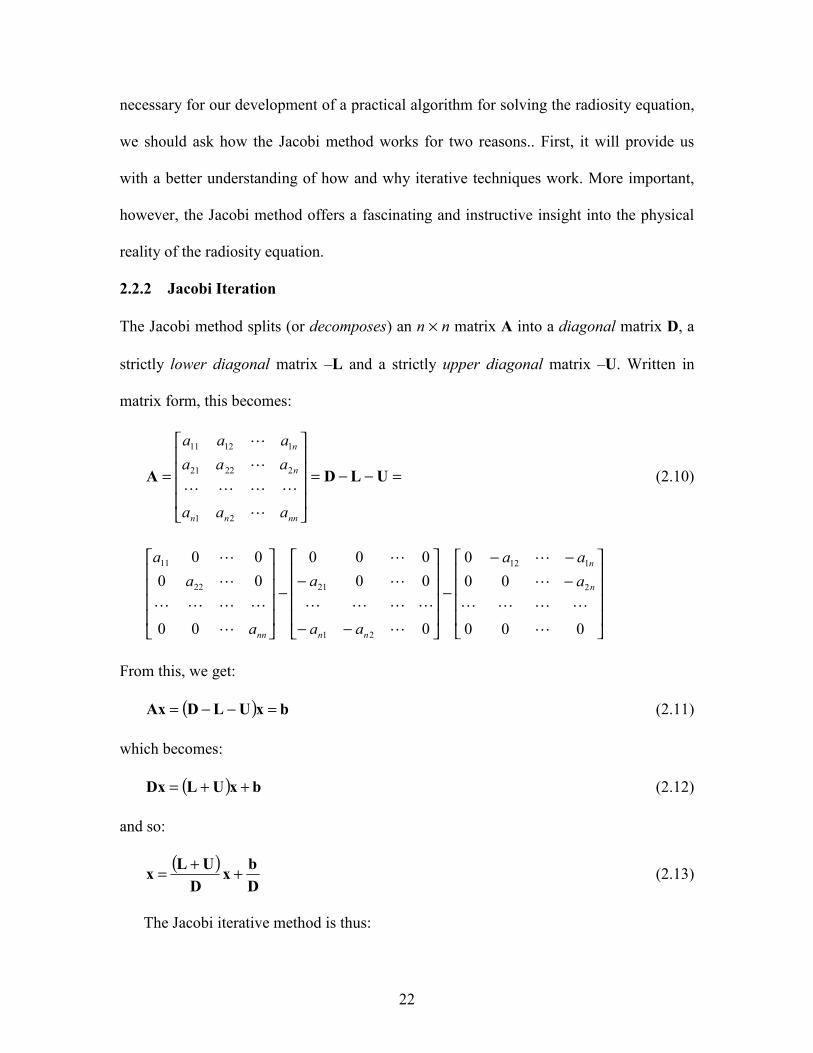
2.2.2 Jacobi Iteration
The Jacobi method splits (or decomposes) an n × n matrix A into a diagonal matrix D, a
strictly lower diagonal matrix –L and a strictly upper diagonal matrix –U. Written in
matrix form, this becomes:
=−−=
= ULDA
nnnn
n
n
aaa
aaaaaa
L
LLLL
L
L
21
22221
11211
(2.10)
−−−
−
−−
−−
000
000
0
00000
00
0000
2
112
21
2122
11
L
LLLL
L
L
L
LLLL
L
L
L
LLLL
L
L
n
n
nnnn
aaa
aa
a
a
aa
From this, we get:
( ) bxULDAx =−−= (2.11)
which becomes:
( ) bxULDx ++= (2.12)
and so:
( )Dbx
DULx ++= (2.13)
The Jacobi iterative method is thus:
23
( ) ( ) ( )Dbx
DULx ++= −1kk (2.14)
or, expressed in its more familiar form:
( )
( )( )ni
a
bxax
ii
i
n
ijj
kjij
ki ,,1,,1
1
K=+−
=∑
≠=
−
(2.15)
In plain English, this equation states that we can solve each element xi(k) of our
approximate solution vector x(k) by using the values of all the other elements xj(k-1) of our
previously calculated solution vector.
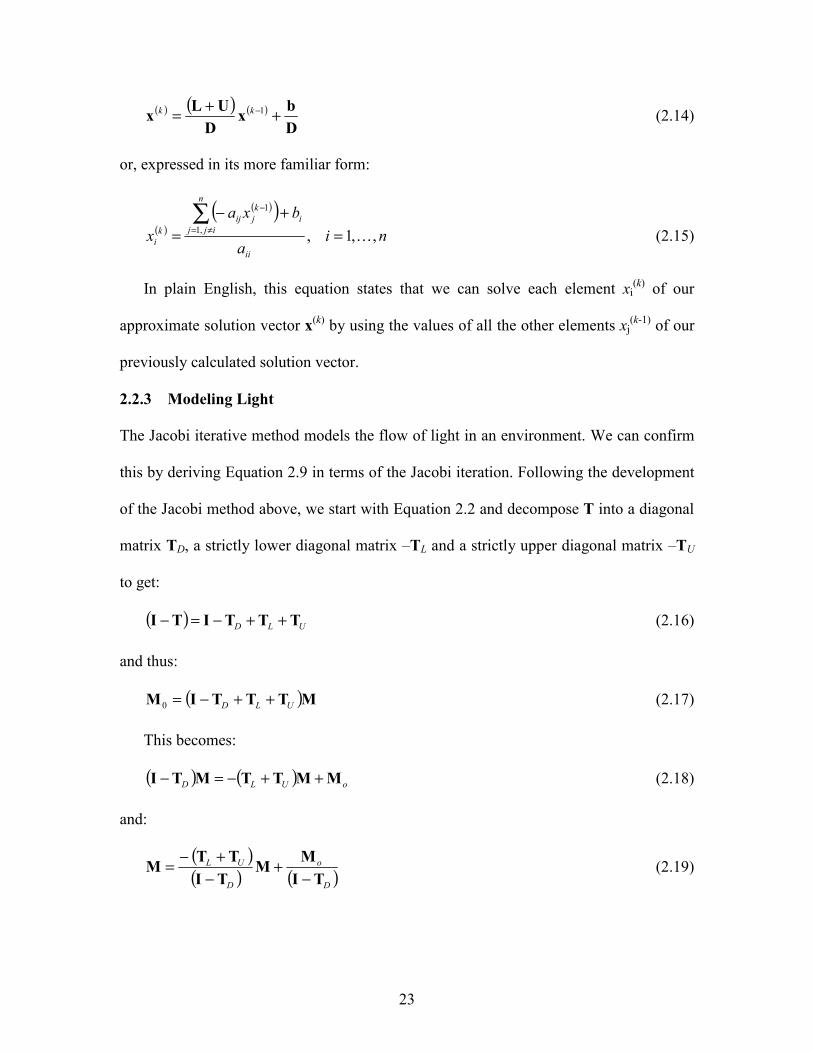
2.2.3 Modeling Light
The Jacobi iterative method models the flow of light in an environment. We can confirm
this by deriving Equation 2.9 in terms of the Jacobi iteration. Following the development
of the Jacobi method above, we start with Equation 2.2 and decompose T into a diagonal
matrix TD, a strictly lower diagonal matrix –TL and a strictly upper diagonal matrix –TU
to get:
( ) ULD TTTITI ++−=− (2.16)
and thus:
( )MTTTIM ULD ++−=0 (2.17)
This becomes:
( ) ( ) oULD MMTTMTI ++−=− (2.18)
and:
( )( ) ( )D
o
D
UL
TIMM
TITTM
−+
−+−= (2.19)
24
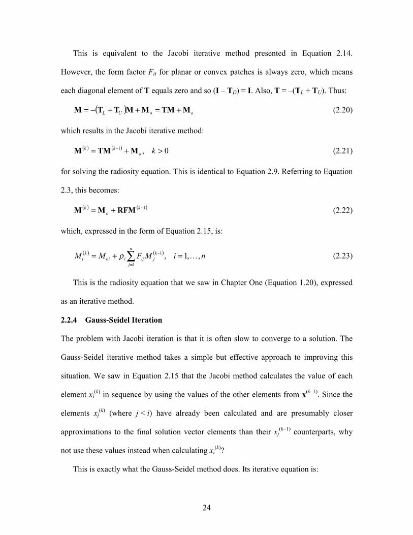
This is equivalent to the Jacobi iterative method presented in Equation 2.14.
However, the form factor Fii for planar or convex patches is always zero, which means
each diagonal element of T equals zero and so (I – TD) = I. Also, T = –(TL + TU). Thus:
( ) ooUL MTMMMTTM +=++−= (2.20)
which results in the Jacobi iterative method:
( ) ( ) 0,1 >+= − kokk MTMM (2.21)
for solving the radiosity equation. This is identical to Equation 2.9. Referring to Equation
2.3, this becomes:
( ) ( )1−+= ko
k RFMMM (2.22)
which, expressed in the form of Equation 2.15, is:
( ) ( ) niMFMM kj
n
jijioi
ki ,,1,1
1
K=+= −
=∑ρ (2.23)
This is the radiosity equation that we saw in Chapter One (Equation 1.20), expressed
as an iterative method.
2.2.4 Gauss-Seidel Iteration
The problem with Jacobi iteration is that it is often slow to converge to a solution. The
Gauss-Seidel iterative method takes a simple but effective approach to improving this
situation. We saw in Equation 2.15 that the Jacobi method calculates the value of each
element xi(k) in sequence by using the values of the other elements from x(k–1). Since the
elements xj(k) (where j < i) have already been calculated and are presumably closer
approximations to the final solution vector elements than their xj(k–1) counterparts, why
not use these values instead when calculating xi(k)?
This is exactly what the Gauss-Seidel method does. Its iterative equation is:
25
( )( )
( )( ) 0,1 >
−+
−= − kkk
LDbx
LDUx (2.24)
or, expressed in its more familiar form:
( )
( ) ( )
nia
bxaxax
ii
i
n
ij
kjij
i
j
kjij
ki ,,1,
11
1K=
+−+−=
∑∑=
−−
= (2.25)
A derivation of Equation 2.24 can be found in most elementary linear algebra and
numerical analysis texts [e.g., burd85].
The Jacobi method can be seen in terms of modeling light bouncing from surface to
surface in an environment. This is not the case for the Gauss-Seidel method. In a sense, it
tries to anticipate the light each surface will receive from the next iteration of reflections.
There is no physical analogue to this process, but it does work in that the Gauss-Seidel
method usually converges more quickly than the Jacobi method does. Cohen and
Greenberg [cohe85] found that the Gauss-Seidel method solved the radiosity equation for
typical environments in six to eight iterations.
2.2.5 Full Radiosity Disadvantages
When it was first introduced to the computer graphics research community by Goral et al.
[gora84] and Nishita and Nakamae [nish85], radiosity rendering was for the most part
viewed as an interesting mathematical curiosity. The Jacobi and Gauss-Seidel methods
have a time complexity of O(n2) for each iteration. Given the available computer
technology at the time, this made the full radiosity algorithm an impractical rendering
technique for all but the simplest of environments.
Another disadvantage of full radiosity is that it requires storage for n2 / 2 form factors
[e.g., Ashd94]. This means that the memory space complexity of the full radiosity
26
algorithm is O(n2) as well. We could possibly avoid this requirement by recomputing
form factors “on the fly” for each patch during each iteration. However, the high cost of
form factor determination (typically 90 percent of the run-time cost) means that we
would have to wait much longer between each iteration. This is exactly what we are
trying to avoid. We need to obtain an initial image as quickly as possible.
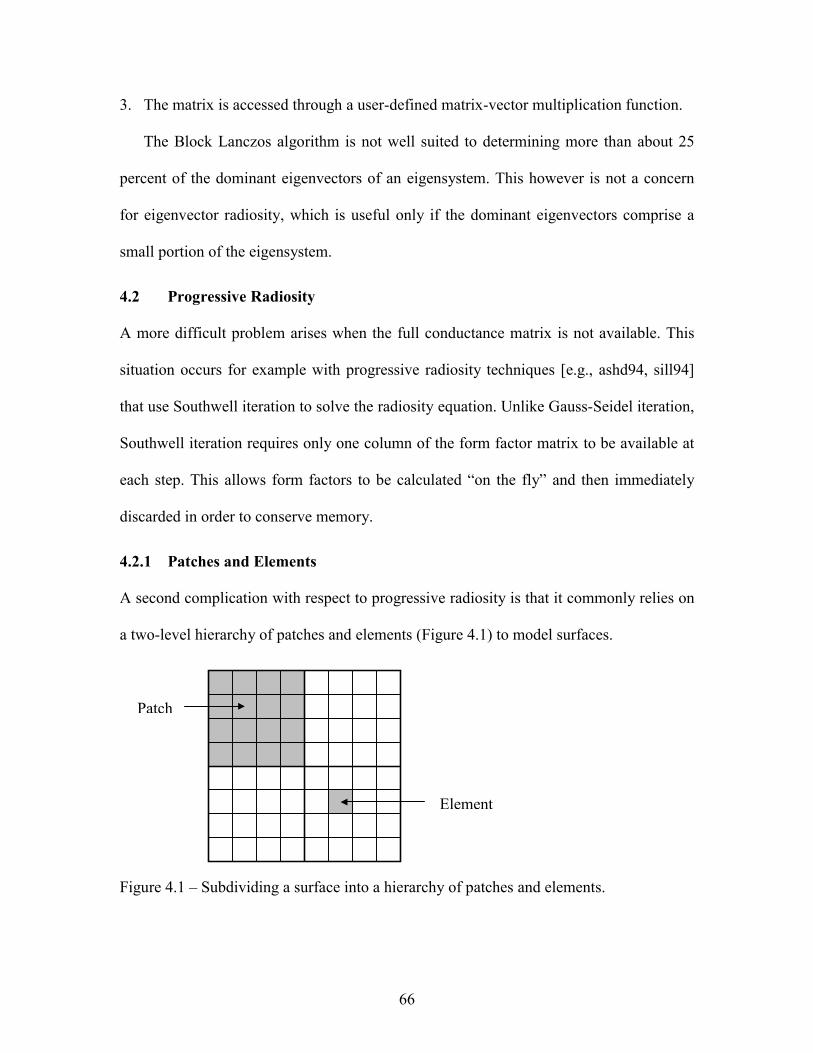
We can gain some relief by substructuring the environment into a two-level hierarchy
of patches and elements [cohe86]. This brings both the time and space complexities down
to O(mn) for n patches and m elements. Substructuring is a useful technique, but we can
do better.
2.3 Shooting Versus Gathering
There is an interesting and instructive physical interpretation of the Jacobi and Gauss-
Seidel methods. We can think of each execution of Equation 2.15 (Jacobi) or 2.25
(Gauss-Seidel) as being one step; it takes n steps to complete one iteration of the method.
At each step, we are updating the estimated exitance of one patch by processing one row
of the radiosity equation. For the Jacobi method, this is Equation 2.23, repeated here as:
( ) ( ) niMFMM kj
n
jijioi
ki ,,1,1
1
K=+= −
=∑ρ (2.26)
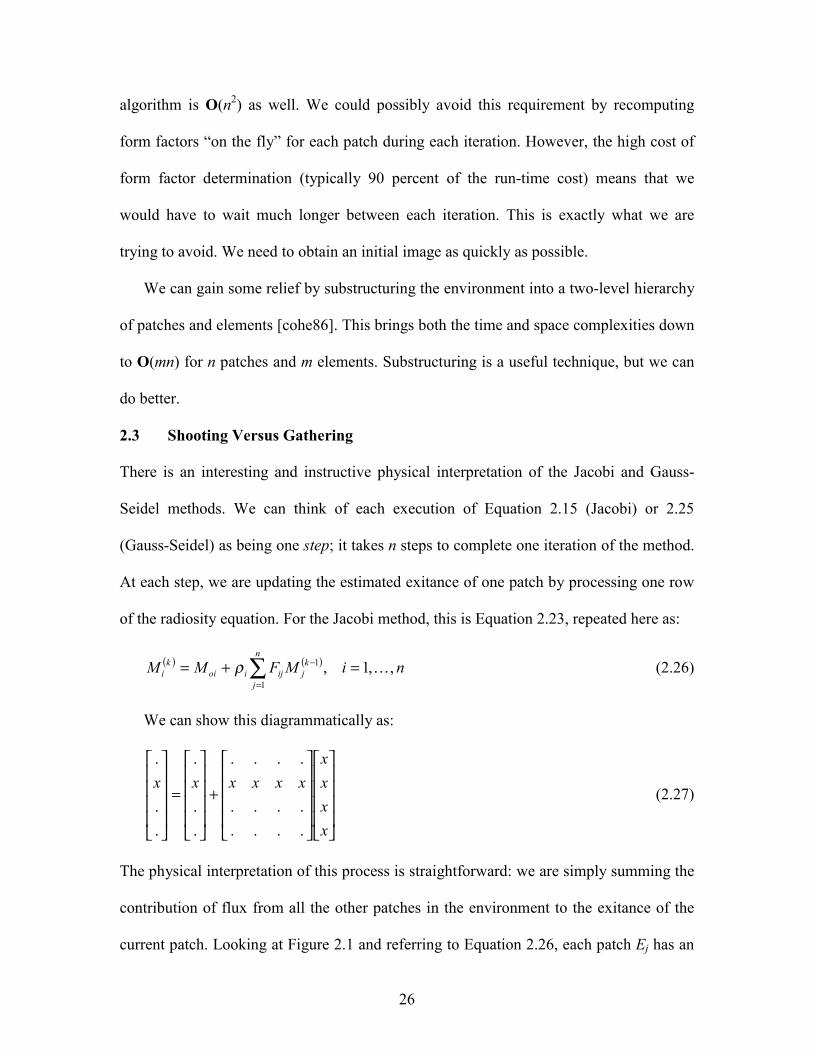
We can show this diagrammatically as:
+
=
xxxx
xxxxxx
....
....
....
.
.
.
.
.
.
(2.27)
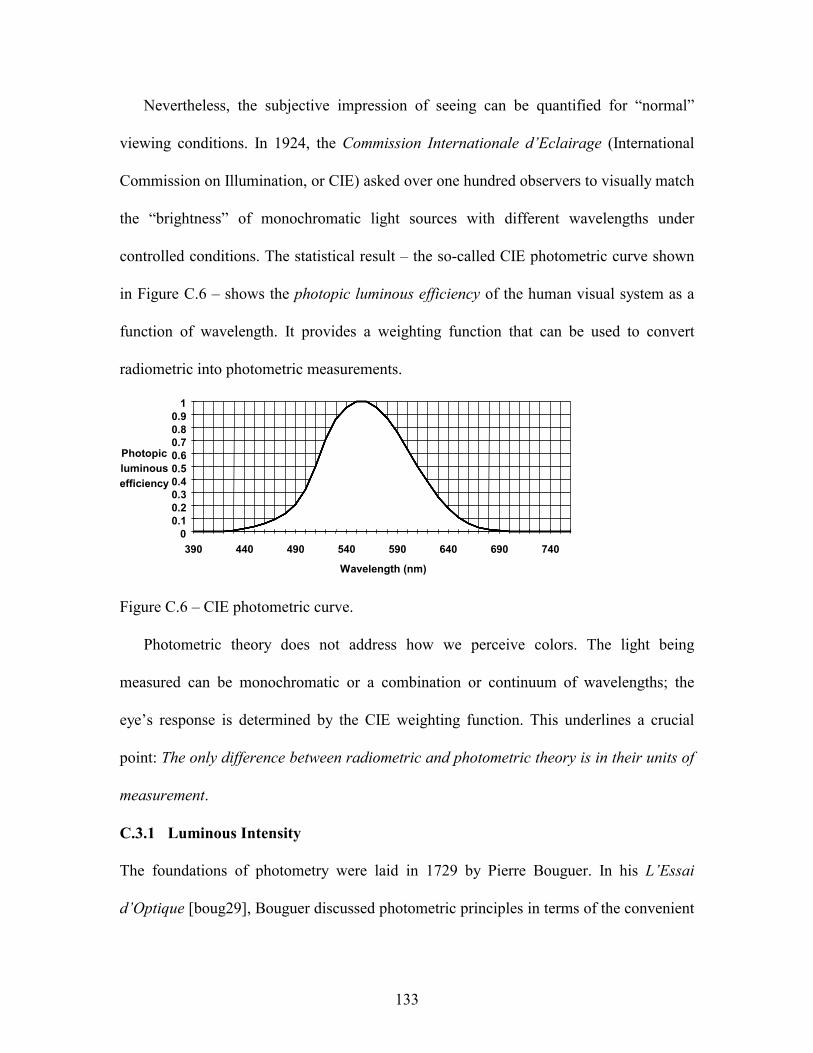
The physical interpretation of this process is straightforward: we are simply summing the
contribution of flux from all the other patches in the environment to the exitance of the
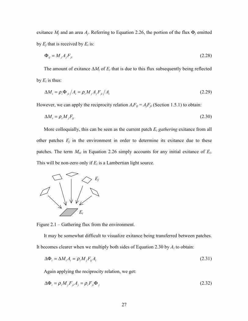
current patch. Looking at Figure 2.1 and referring to Equation 2.26, each patch Ej has an
27
exitance Mj and an area Aj. Referring to Equation 2.26, the portion of the flux Φj emitted
by Ej that is received by Ei is:
jijjij FAM=Φ (2.28)
The amount of exitance ∆Mi of Ei that is due to this flux subsequently being reflected
by Ei is thus:
ijijjiijiii AFAMAM ρρ =Φ=∆ (2.29)
However, we can apply the reciprocity relation AiFij = AjFji (Section 1.5.1) to obtain:
ijjii FMM ρ=∆ (2.30)
More colloquially, this can be seen as the current patch Ei gathering exitance from all
other patches Ej in the environment in order to determine its exitance due to these
patches. The term Moi in Equation 2.26 simply accounts for any initial exitance of Ei.
This will be non-zero only if Ei is a Lambertian light source.
Figure 2.1 – Gathering flux from the environment.
It may be somewhat difficult to visualize exitance being transferred between patches.
It becomes clearer when we multiply both sides of Equation 2.30 by Ai to obtain:
iijjiiii AFMAM ρ=∆=∆Φ (2.31)
Again applying the reciprocity relation, we get:
jjiijjijii FAFM Φ==∆Φ ρρ (2.32)
Ej
Ei
28
which shows that we are in fact gathering and subsequently reflecting radiant flux.
Equation 2.30 is more useful in terms of Equation 2.26, however, and so we “gather”
exitance to Ei. The difference is solely semantic.
A number of authors have loosely referred to this process as gathering “energy.”
However, the physical quantity being discussed is radiant exitance (i.e., watts per unit
area) times area. This is power, or radiant flux. Energy is “gathered” only in the sense
that solving the radiosity equation balances the flow of energy (which is power) between
elements in the environment.
The problem with this approach is that it can be excruciatingly slow. Consider a
complex environment with perhaps 50,000 patches. Using the Jacobi or Gauss-Seidel
method, we must perform one complete iteration before we have an image of the first
bounce of light from the environment. That means we must execute Equation 2.26 50,000
times! This clearly does not satisfy our requirement for an “immediate but approximate”
image.
This is where the physical interpretation becomes useful. If we think for a moment
about how light flows in an environment, it becomes evident that we should be interested
in those elements that emit or reflect the most light. It logically does not matter in what
order we consider the distribution of light from patch to patch, as long as we eventually
account for it being completely absorbed.
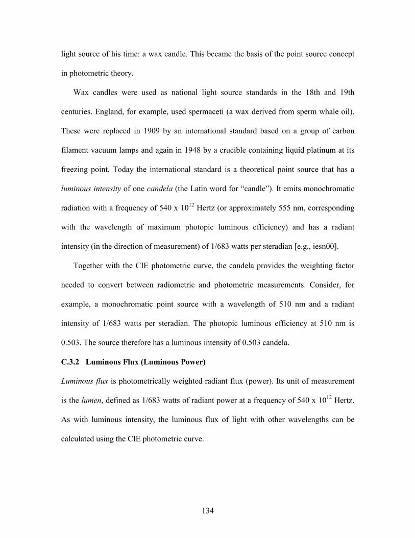
This leads to an entirely different paradigm. Given an environment with one or more
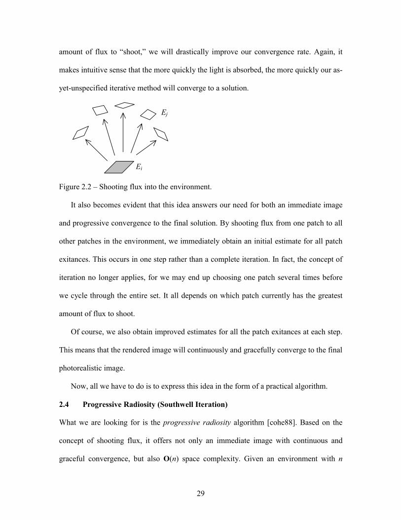
light sources, we can think of them shooting flux to the other patches (Figure 2.2). These
patches then become in effect secondary light sources, shooting some of the flux they
receive back into the environment. By always selecting the patch that has the greatest
29
amount of flux to “shoot,” we will drastically improve our convergence rate. Again, it
makes intuitive sense that the more quickly the light is absorbed, the more quickly our as-
yet-unspecified iterative method will converge to a solution.
Figure 2.2 – Shooting flux into the environment.
It also becomes evident that this idea answers our need for both an immediate image
and progressive convergence to the final solution. By shooting flux from one patch to all
other patches in the environment, we immediately obtain an initial estimate for all patch
exitances. This occurs in one step rather than a complete iteration. In fact, the concept of
iteration no longer applies, for we may end up choosing one patch several times before
we cycle through the entire set. It all depends on which patch currently has the greatest
amount of flux to shoot.
Of course, we also obtain improved estimates for all the patch exitances at each step.
This means that the rendered image will continuously and gracefully converge to the final
photorealistic image.
Now, all we have to do is to express this idea in the form of a practical algorithm.
2.4 Progressive Radiosity (Southwell Iteration)
What we are looking for is the progressive radiosity algorithm [cohe88]. Based on the
concept of shooting flux, it offers not only an immediate image with continuous and
graceful convergence, but also O(n) space complexity. Given an environment with n
Ej
Ei
30
patches, it requires memory space for only n form factors. Even better, it can generate an
initial image almost immediately, and can generate if necessary updated images after
each step (as opposed to each iteration).
So how does it work? To shoot flux or exitance back into the environment, we simply
reverse the subscripts of Equation 2.30. For exitance, this becomes:
jiijj
iijijj FM
AAFMM ρρ ==∆ (2.33)
Multiplying both sides of this equation by the area of patch Ej gives us the equation for
shooting flux.
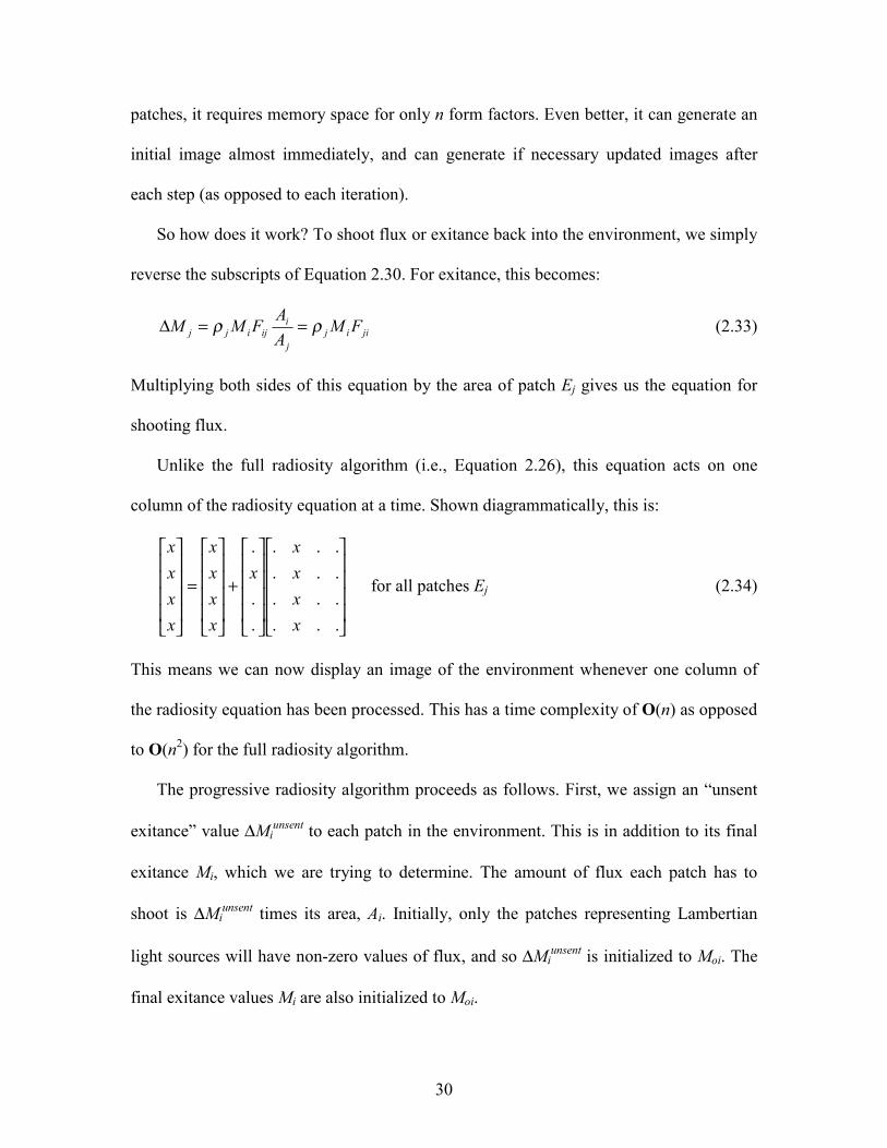
Unlike the full radiosity algorithm (i.e., Equation 2.26), this equation acts on one
column of the radiosity equation at a time. Shown diagrammatically, this is:
+
=
...
...
...
...
.
.
.
xxxx
x
xxxx
xxxx
for all patches Ej (2.34)
This means we can now display an image of the environment whenever one column of
the radiosity equation has been processed. This has a time complexity of O(n) as opposed
to O(n2) for the full radiosity algorithm.
The progressive radiosity algorithm proceeds as follows. First, we assign an “unsent
exitance” value ∆Miunsent to each patch in the environment. This is in addition to its final
exitance Mi, which we are trying to determine. The amount of flux each patch has to
shoot is ∆Miunsent times its area, Ai. Initially, only the patches representing Lambertian
light sources will have non-zero values of flux, and so ∆Miunsent is initialized to Moi. The
final exitance values Mi are also initialized to Moi.
31
Choosing the patch Ei with the greatest amount of flux (not exitance) to shoot, we
execute Equation 2.33 for every other patch Ej in the environment. Each of these patches
“receives” a delta exitance ∆Mj; this value is added to both its unsent exitance ∆Mjunsent
and its final exitance Mj.
After the flux has been shot to every patch Ej, ∆Miunsent is reset to zero. This patch can
only shoot again after receiving more flux from other patches during subsequent steps.
This process continues until the total amount of flux remaining in the environment is
less than some predetermined fraction ε of the original amount, or:
ε≤∆∑=
n
ii
unsenti AM
1
(2.35)
At this point, the algorithm is considered to have converged to a solution.
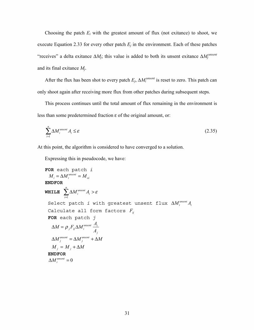
Expressing this in pseudocode, we have:
FOR each patch i oi
unsentii MMM =∆=
ENDFOR
WHILE ε>∆∑=
n
ii
unsenti AM
1
Select patch i with greatest unsent flux iunsenti AM∆
Calculate all form factors ijF
FOR each patch j
j
iunsentiijj A
AMFM ∆=∆ ρ
MMM unsentj
unsentj ∆+∆=∆
MMM jj ∆+=
ENDFOR 0=∆ unsent
iM
32
ENDWHILE
Figure 2.3 – Progressive radiosity algorithm
Progressive radiosity does not – repeat, does not – require any less time to completely
solve the radiosity equation to some vanishingly small margin of error. It is an iterative
approach that, like full radiosity, progressively refines the patch exitances as it converges
to a solution. However, its overwhelming advantage is that usable images can be
displayed almost immediately, and that each succeeding image takes much less time to
calculate.
We still have the form factors to contend with. However, we only need to calculate
the n form factors Fij from the current patch Ei to all other patches Ej between displaying
images. We have to recompute these form factors on the fly for each step of the
progressive radiosity algorithm. However, the convergence rate is much faster than it is
for full radiosity. Cohen et al. [cohe88] compared progressive refinement and full
radiosity algorithms using an environment consisting of 500 patches and 7,000 elements.
The progressive radiosity implementation converged to a visually acceptable image after
approximately 100 steps. At this point, the full radiosity implementation was only 20
percent of its way through its first iteration.
Gortler and Cohen [gort93] established that the progressive radiosity algorithm is a
variant of the Southwell iteration method [e.g., gast70]. Like the Jacobi and Gauss-Seidel
methods, Southwell iteration will always converge to a solution for any physically
possible radiosity equation.
2.5 Convergence Behaviour
Shao and Badler [shao93] presented a detailed and informative discussion of the
convergence behavior of the progressive refinement radiosity algorithm. They observed
33
that while the algorithm may quickly converge to a visually appealing image, many more
steps are often required to capture the nuances of color bleeding and soft shadows. They
demonstrated that it took 2,000 or more steps to achieve full convergence in a complex
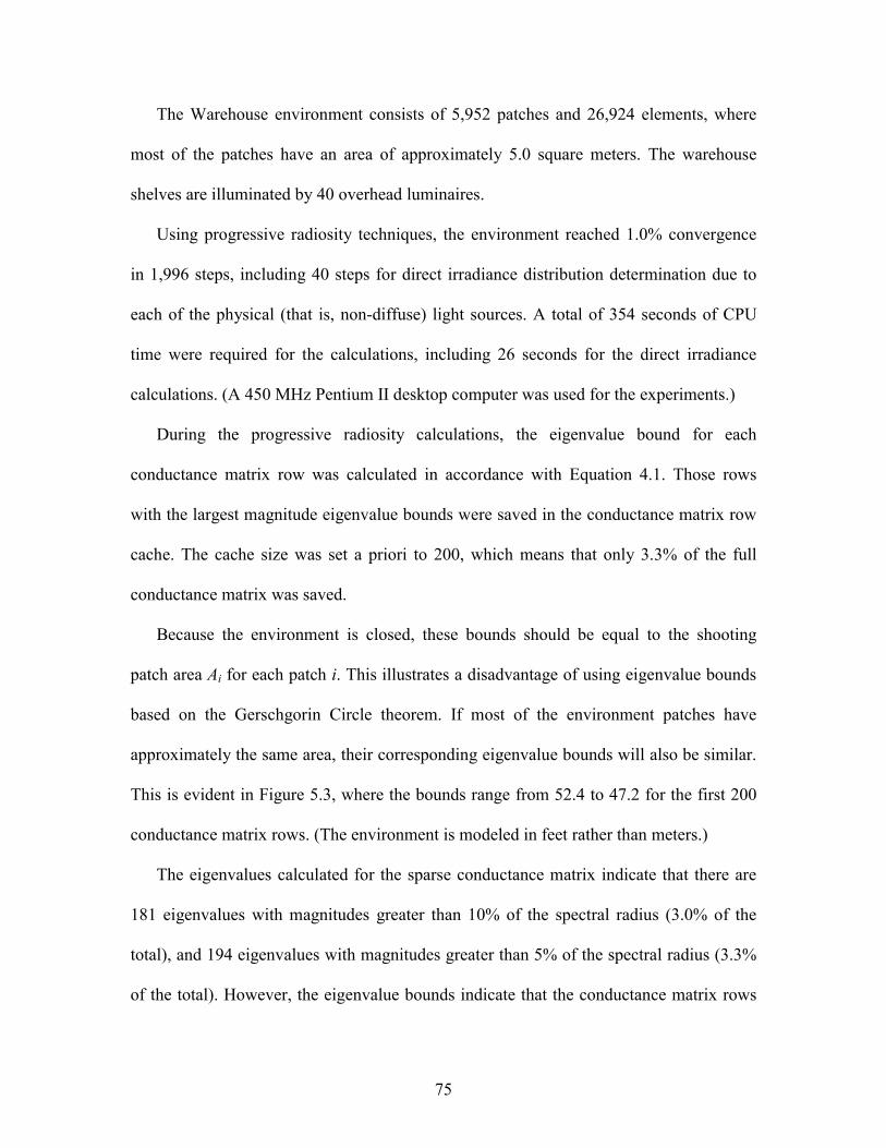
environment of some 1,000 patches.
Much of the problem lies in how progressive refinement works. By always selecting
the patch with the most flux to shoot, it concentrates first on the light sources. Most of
their flux will be shot to what Shao and Badler called global patches – those patches
which are relatively large and can be seen from much of the environment. For an
architectural interior, these are typically the walls, floor and ceiling of a room. Their
patches receive most of the flux from the light sources and consequently shoot it to the
other global patches.
The local patches are those patches which are small and are usually hidden from
much of the environment. Their flux will not be shot until that of the global patches has
been exhausted. This is undesirable for two reasons. First, their small areas means that
they will receive relatively little flux in comparison to the global patches. It may take
several hundred steps before they shoot for the first time.
The second reason is that when these local patches do shoot, much of their flux often
goes no further than their immediate neighbors. While this does not affect the global
environment to any great extent, it does account for color bleeding and soft shadow
effects. In this sense, a better error metric is the worst-case difference between the
estimated and converged element exitances. In their experiments, Shao and Badler
observed that it took twice as many iterations as there were patches in the environment.
34
One strategy to overcome this problem involves de-emphasizing the contributions due
to the global patches, ensuring that all patches shoot their flux in a reasonable number of
steps. This requires a modification of the progressive refinement radiosity algorithm that
is described next.
2.6 Positive Overshooting
Convergence of the Gauss-Seidel algorithm can often be accelerated by using one of
several techniques known as successive overrelaxation [e.g., nobl69]. Applied to the
radiosity equation, these techniques can be interpreted as “overshooting” the amount of
flux from a patch into the environment. That is, the amount of flux shot from the patch is
more than the amount of unsent flux the patch actually has. The flux shot in subsequent
steps by the receiving patches will tend to cancel this overshooting. In the meantime, the
total amount of unsent flux in the environment is shot and absorbed more quickly. This
tends to result in faster convergence rates.
Shao and Badler [shao93] presented a modified version of the progressive refinement
radiosity algorithm that incorporates positive overshooting to accelerate the convergence
rate by a factor of two or more. At the same time, it tends to prioritize the ordering of
patches being shot such that the local patches are shot sooner, thereby enhancing the
rendering of subtle lighting effects such color bleeding and soft shadows.
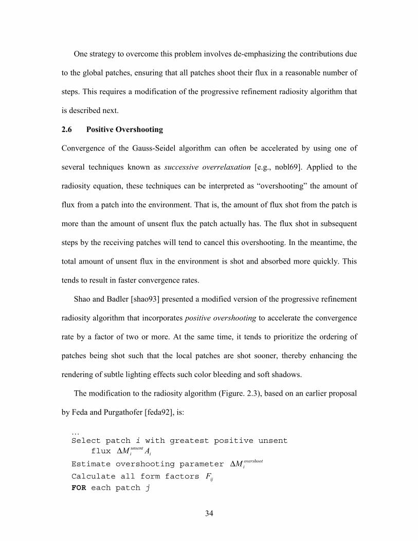
The modification to the radiosity algorithm (Figure. 2.3), based on an earlier proposal
by Feda and Purgathofer [feda92], is:
… Select patch i with greatest positive unsent flux i
unsenti AM∆
Estimate overshooting parameter overshootiM∆
Calculate all form factors ijF
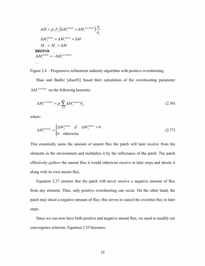
FOR each patch j
35
( )j
iovershooti
unsentiijj A
AMMFM ∆+∆=∆ ρ
MMM unsentj
unsentj ∆+∆=∆
MMM jj ∆+=
ENDFOR overshooti
unsenti MM ∆−=∆
…
Figure 2.4 – Progressive refinement radiosity algorithm with positive overshooting
Shao and Badler [shao93] based their calculation of the overshooting parameter
overshootiM∆ on the following heuristic:
ij
n
j
unsentji
overshooti FMM ∑
=
′∆=∆1
ρ (2.36)
where:
>∆∆
=′∆otherwise0
0unsentj
unsentjunsent
j
MifMM (2.37)
This essentially sums the amount of unsent flux the patch will later receive from the
elements in the environment and multiplies it by the reflectance of the patch. The patch
effectively gathers the unsent flux it would otherwise receive in later steps and shoots it
along with its own unsent flux.
Equation 2.37 ensures that the patch will never receive a negative amount of flux
from any element. Thus, only positive overshooting can occur. On the other hand, the
patch may shoot a negative amount of flux; this serves to cancel the overshot flux in later
steps.
Since we can now have both positive and negative unsent flux, we need to modify our
convergence criterion. Equation 2.35 becomes:
36
ε≤∆∑=
n
ii
unsenti AM
1
(2.38)
Experiments performed by Shao and Badler on two complex environments
demonstrated that the convergence rate with positive overshooting can be accelerated by
a factor of two or more over that of conventional progressive radiosity. There was also
strong evidence that the appearance of subtle color bleeding and soft shadow effects may
appear as much as three to five times more quickly. Positive overshooting is clearly a
useful addition to the basic progressive radiosity algorithm.
Other overrelaxation techniques for solving the radiosity equation are described by
Gortler and Cohen [gort93] and Greiner et al. [grei93].
2.7 Environment Changes
Progressive radiosity is typically used to calculate the radiant flux distribution of static
environments. If the initial distribution is changed (by changing or repositioning the light
sources) or the surface reflectances are modified, the radiosity solution for the
environment has to be recalculated.
2.7.1 Changes in Lighting
Suppose we want to change or reposition the light sources. The form factor matrix will
remain unchanged, but this is little consolation where progressive radiosity is concerned.
In general, we have to solve the radiosity equation, form factors and all, whenever the
initial exitance due to a light source is changed.
If the changes are relatively minor, we can use the final exitance vector of the
previous solution as the initial exitance vector Mo. In most cases, progressive radiosity
will quickly converge to the new solution. (At worst, Mo will be no different than a
random estimate, and progressive radiosity will eventually converge.)
37
Of course, if any of the light sources are dimmed, this will imply a negative quantity
of unsent exitance [chen90]. Several minor changes to the progressive radiosity equation
algorithm presented in Figure 2.3 will be needed to accommodate this physically
impossible but eminently useful possibility.
If there are many lighting changes to be modeled – theatre lighting, for example – it
may be useful to calculate separate solutions for each individual group of light sources
[aire90]. These solutions are independent of one another, and can be scaled and summed
to represent any possible combination of light sources and their final exitances.
Another approach is to precalculate a set of solutions for a range of initial radiant flux
distributions and decompose them into a series of basis functions [nime94, doba97]. This
is useful mostly for image synthesis of outdoor environments and daylighting analysis,
where numerous solar positions must be accounted for. Approximate solutions for
intermediate solar positions that have not been previously calculated can be obtained
through blending of the basis functions.
The difficulty with this approach is that it is difficult to determine a priori how many
solar positions need to be calculated to obtain a reasonable set of basis functions. In
particular, it does not take into account the geometry of the environment – a small change
in solar position may produce drastically different final radiant exitance distributions.
2.7.2 Changes in Surface Reflectances
A second challenge comes when the surface reflectances are changed. One typical
example is in architectural design where the designer may want to compare the visual
appearance and effect of different wall or floor finishes. Again, the form factor matrix
38
remains unchanged. However, the solution may change drastically if the surface area is
large and its reflectance is changed by any significant amount.
Chen [chen90] noted that the previous solution often provides a satisfactory initial
exitance vector Mo, particularly when the number of surfaces whose reflectances have
been changed is small in number. From Equation 1.20, we know that the exitance of a
surface patch is given by:
ij
n
jjioii FMMM ∑
=
+=1
ρ (2.39)
If we define M′oi as the new initial exitance and ρ′i as the new surface reflectance,
then the incremental change in final exitance is given by:
( ) ij
n
jjiioioii FMMMM ∑
=
−′+−′=∆1
ρρ (2.40)
Substituting Equation 2.36 into this equation gives us:
( )( )i
oiiiioioii
MMMMMρ
ρρ −−′+−′=∆ (2.41)
where the previous surface reflectance ρi is assumed to be greater than zero. We can add
this value (which may be negative) to the current calculated patch exitance Mi and also its
remaining unsent exitance (if any). From this, we can shoot the exitance until the
radiosity algorithm converges to a new solution.
This approach does not however help when there are significant changes to the
surface reflectances. As with changes to the light sources, major changes often result in
completely different final exitance distributions. Calculating these distributions often
takes as much effort when using the previous solution as when using the initial radiant
flux distribution Moi.
39
2.8 A New Approach
While progressive radiosity is a useful technique for producing architectural
visualizations and generating photometric predictions for static environments, it requires
too much computational effort to determine the effect of significant changes in the
lighting or surface reflectances. The next chapter will introduce a new approach to
solving the radiosity equation that addresses this problem.
40
Chapter 3
Eigenvector Radiosity – Theory
3.1 Eigenanalysis
Eigenanalysis is a well-known technique with many scientific and engineering
applications, including structural vibration analysis, electrical power system stability,
pattern recognition, radar and acoustic signal processing, quantum mechanics, and much
more. As an analysis tool, it identifies the principal vibrational modes (or their abstract
analogues) of a physical system. As a computational tool, it offers time and space savings
by providing approximate solutions using only the principal modes.
Applying eigenanalysis techniques to a problem domain generally requires that the
physical meaning of the resultant eigensystem be known. In the example of structural
vibration analysis, eigenanalysis of the stiffness matrix associated with a finite element
model identifies the natural vibration modes and frequencies of the structure. However,
the physical meaning of eigenanalysis in terms of the radiosity equation has been an open
question for the past sixty years.
3.1.1 The Radiosity Kernel
Moon [moon40] appears to have been the first researcher to consider this question. He
noted that the continuous form of the radiosity equation could be expressed as a
Fredholm integral equation of the second kind:
( ) ( ) ( ) ( ) yyxyxx dKMMMS
o ,∫+= λ (3.1)
41
where ( )xoM is the initial exitance at point x on a surface in the environment S, ( )xM is
the final exitance at point x, ( )yM is the final exitance at point y, λ is a constant, and the
radiosity kernel ( )yx,K is integrated over all surfaces.
Moon also noted that the associated homogeneous equation:
( ) ( ) ( ) yyxyx dKMMS
,∫=′ λ (3.2)
has solutions K,, 21 MMM ′′=′ that are its eigenfunctions, with corresponding eigenvalues
K,, 21 λλλ = Once these functions are found for a given radiosity kernel, the solution for
Equation 3.1 can be determined.
Moon was able to develop closed-form analytic solutions for a number of simple
environments, including the sphere, infinite cylinder, and parallel and perpendicular
plates. He later expanded on this work with his co-author Spencer in their book, “The
Photic Field” [moon81]. However, each kernel required its own analysis, and so the
eigenanalysis of arbitrary environments was still an open problem.
Koenderink and van Doorn [koen83] examined eigenfunctions of the radiosity kernel
from the perspective of computer vision research. Given a complex geometric object such
as a marble bust with Lambertian surfaces, the radiosity equation models the multiple
interreflections of flux between these surfaces. Koenderink and van Doorn demonstrated
that the eigenfunctions of the radiosity kernel describe “geometrical modes” that are
dependent on the object geometry and invariant with respect to the initial irradiance.
These modes were interpreted as pseudofacets on an equivalent convex object.
Langer [lang98] extended the work of Koenderink and van Doorn by examining the
relationship between interreflections and shadows. He noted that the geometrical mode
42
corresponding to the eigenfunction of the radiosity kernel with the largest magnitude
eigenvalue is a non-negative function that is physically realizable. Langer called this the
“principal mode” of the environment. Further, given an environment with constant
surface reflectance throughout, the principal mode is constant over x, and may be
interpreted as the “ambient light” term used in computer graphics. (This was also noted
by Moon in [moon40].)
3.1.2 The Radiosity Matrix
Baranoski et al. [bara97] and Baranoski [bara98] attempted to elucidate the physical
significance of the radiosity matrix eigensystem by interpreting and visualizing the
eigenvectors with the largest and smallest eigenvalues as patch exitance vectors. (The
exitance vector elements were interpreted as patch luminances, which after appropriate
shifting and scaling allowed images of the environments to be displayed.)
These authors also investigated the dominant eigenvectors of the “symmetric”
radiosity matrix formed by multiplying the radiosity matrix by a diagonal matrix whose
elements consisted of the quotient of the patch areas and their reflectances.
Unfortunately, qualitative analysis of the images proved inconclusive. The authors
inferred some general properties relating to the flow of light within simple environments,
but were unable to offer any quantitative physical interpretation of their results.
Ramamoorthi [rama99] performed similar experiments on the symmetric radiosity
matrix, but for more complex environments with 2,600 and 4,500 patches. In addition to
visualizing the individual eigenvectors (which he called “eigenmodes”), he generated
visualizations using only the dominant eigenvectors.
43
Ramamoorthi noted that only a small fraction of the eigenvectors had significant
eigenvalues. For the larger environment (a room with a table and four chairs), fewer than
20 of the 4,500 eigenvalues exceeded 10 percent of the spectral radius. A reasonably
accurate (in the sense of 2-norm relative error) global approximation could be obtained
with as few as 10 of the 4,500 eigenvectors. However, it required 150 to 200 eigenvectors
to provide patch exitances that were locally accurate. (That is, where both the 2-norm and
∞-norm relative errors for the patch exitance vector were small.)
3.1.3 The Form Factor Matrix
Finally, DiLaura and Franck [dila93] demonstrated that the iterative formulation of the
radiosity equation (Equation 2.22) could be reformulated in terms of the eigensystem of
the form factor matrix. Unfortunately, their technique applied only to symmetric form
factor (not radiosity) matrices, which generally occur only in unoccluded environments
where all surface patches are the same size.
This leaves open the fundamental question: What is the physical significance of the
eigensystem of a form factor (or radiosity) matrix? Curiously, the answer involves a
physical analogy of radiative transfer systems that has been completely ignored for the
past forty or so years.
3.2 Radiative Transfer Networks
Suppose we are given a system of n discrete surface patches Ai with Lambertian
reflectance ρi, irradiance Ei, and possibly zero initial radiant exitance Moi for each patch i.
The radiosity equation:
∑=
+=+=n
jjijioiiioii MFMEMM
1
ρρ (3.3)
44
describes the final radiant exitance Mi of each patch i, where Fij is the form factor from
patch i to patch j, and where E and M are assumed to be constant over each patch.
Expressed in matrix form, this becomes:
RFMMREMM +=+= oo (3.4)
where M is the final radiant exitance vector, Mo is the initial radiant exitance vector, E is
the irradiance vector, R is the diagonal reflectance matrix (where Rii = ρi and Rij = 0, i ≠
j), and F is the form factor matrix.
Rearranged slightly, this becomes:
( )MRFIM −=o (3.5)
which is the familiar matrix form of the radiosity equation.
As shown by Oppenheim [oppe54, oppe56] and O’Brien [obri55], the radiative flux
transfer between these patches can be described in terms of a linear resistive network
with one or more voltage sources. For a given patch Ai, the net flux transfer away from
the patch is given by:
( )iiineti EMA −=Φ (3.6)
which is analogous to current in an electrical circuit.
Substituting Ei from Equation 3.3 into Equation 3.6 gives:
( )( )
−
−−
=Φ ii
oi
i
iineti M
MAρρ
ρ1
1 (3.7)
where from Ohm’s Law [e.g., thom94], the term ( )
−
− ii
oi MM
ρ1 is analogous to voltage,
and the term ( )
i
iiAρ
ρ−1 is analogous to conductance (i.e., the inverse of resistance).
45
Now to conserve energy in the system, the summation relation must hold for each
patch Ai:
∑=
=n
jijF
1
1 (3.8)
This means that if the system is not fully enclosed, it must be enclosed in a box whose
interior surfaces have zero reflectance and zero initial radiant exitance. This box will act
as an energy sink to maintain the energy balance.
Therefore, by again substituting Ei from Equation 3.3 into Equation 3.6, we also have:
( )∑=
−=Φn
jjiiji
neti MMFA
1
(3.9)
which gives:
( ) ( )( )
−
−−
=−∑=
ii
oi
i
iin
jjiiji M
MAMMFA
ρρρ
11
1
(3.10)
This is analogous to Kirchoff’s Current Law [e.g., thom94], which states that the
algebraic sum of the currents entering a node in an electrical circuit is always zero.
This completes the analogy: each patch represents a node in an electrical circuit, with
radiative flux (current) flowing between these patches (nodes). The amount of flux is
determined by the analogies of voltage and conductance.
Figure 3.1 shows as an example the RT network for an enclosed system defined by
three surface patches with finite width and infinite length. The conductances go1, go2, and
go3 represent the initial radiant exitances, and have the form:
( )i
iioi
Ag
ρρ−
=1
(3.11)
46
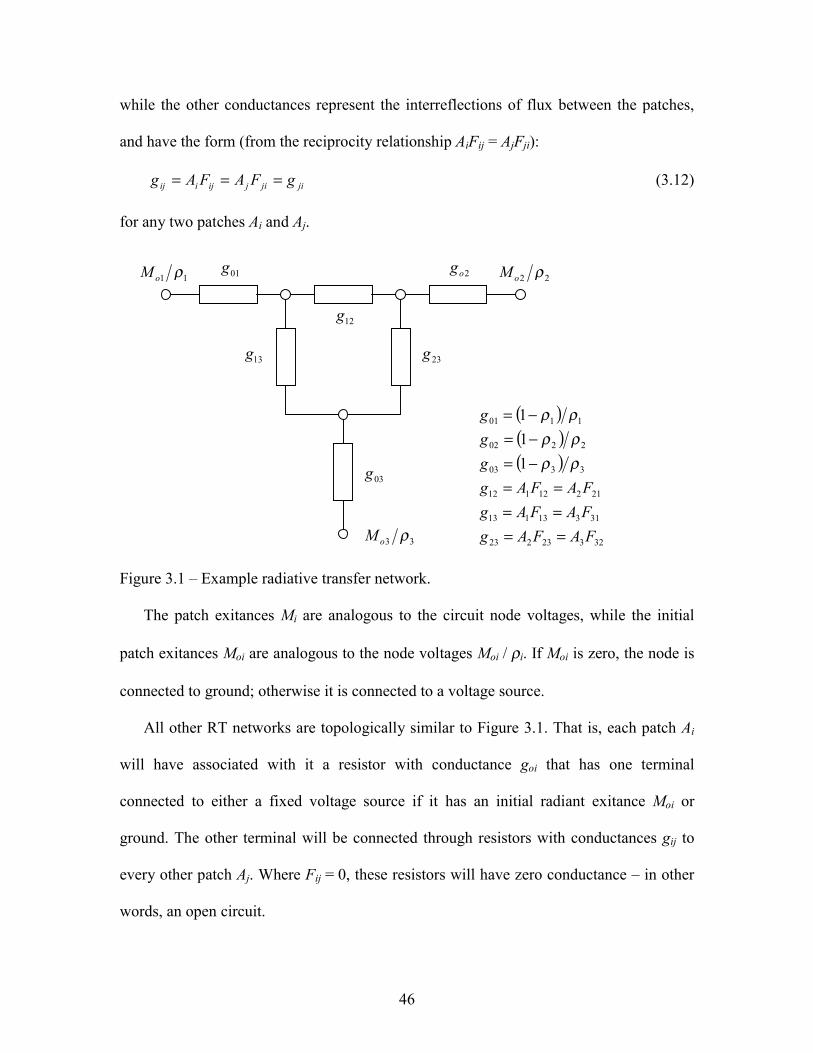
while the other conductances represent the interreflections of flux between the patches,
and have the form (from the reciprocity relationship AiFij = AjFji):
jijijijiij gFAFAg === (3.12)
for any two patches Ai and Aj.
Figure 3.1 – Example radiative transfer network.
The patch exitances Mi are analogous to the circuit node voltages, while the initial
patch exitances Moi are analogous to the node voltages Moi / ρi. If Moi is zero, the node is
connected to ground; otherwise it is connected to a voltage source.
All other RT networks are topologically similar to Figure 3.1. That is, each patch Ai
will have associated with it a resistor with conductance goi that has one terminal
connected to either a fixed voltage source if it has an initial radiant exitance Moi or
ground. The other terminal will be connected through resistors with conductances gij to
every other patch Aj. Where Fij = 0, these resistors will have zero conductance – in other
words, an open circuit.
11 ρoM 22 ρoM
33 ρoM
01g
03g
23g
2og
13g
12g
( )( )( )
32323223
31313113
21212112
3303
2202
1101
111
FAFAgFAFAgFAFAg
ggg
======
−=−=−=
ρρρρρρ
47
The RT network analogy represents an environment solely in terms of radiative flux
transfer between its surface patches. If we are interested in simplifying an environment to
reduce the computational effort needed to solve its radiosity equation, then it is
reasonable to begin with its RT network.
3.3 Symmetric Matrices
From Equation 3.10 we can derive these simultaneous linear equations [obri55]:
n
nNNNNN
n
onn
nno
nno
MAMAFMAFMA
MAFMAMAFMA
MAFMAFMAMA
ρρ
ρρ
ρρ
+−−=
−+−=
−−=
L
L
L
L
2211
222
221221
2
22
1121121
11
1
11
(3.13)
Expressed in matrix form, these become:
( )MRFIARMAR −= −− 11o (3.14)
which is equivalent to Equation 3.5. As noted by Nievergelt [niev97], multiplying both
sides of Equation 3.5 by AR–1 in Equation 3.14 replaces exitances with equivalent radiant
fluxes that produce the same exitances from the system’s Lambertian surface patches.
Neumann [neum94] and Nievergelt [niev97] both noted that this operation produces a
version of the radiosity matrix AR–1 (I – RF), which is symmetric positive definite.
Trivially rearranging terms in Equation 3.4, we also have:
( ) SGMMMAFRAMM +=+= −oo
1 (3.15)
where with reference to radiative transfer networks, the matrix G is the symmetric
conductance matrix for the interconnected conductances gij.
48
3.4 Spectral Decomposition
Given any square n × n matrix B, the spectral decomposition theorem [e.g., deif91] states
that:
∑=
==n
iiii
1
** vvVDVB λ (3.16)
where ( )nvvV ,,1 K= is a matrix of the orthonormalized eigenvectors of B,
( )ndiag λλ ,,1 K=D is a diagonal matrix of their associated eigenvalues, and *ii vv is the
ith eigenprojection of B corresponding to the eigenvalue λi.
In many cases, the matrix B can be approximated by a subset of the eigenvectors with
the largest magnitude eigenvalues. That is, if the eigenvectors are ordered such that
nλλλ ≥≥≥ K21 , then:
npp
iiii <<=′≈ ∑
=
,1
*vvBB λ (3.17)
where B' is rank deficient. (For a symmetric matrix, the complex conjugate vector *iv
becomes the transpose vector Τiv .)
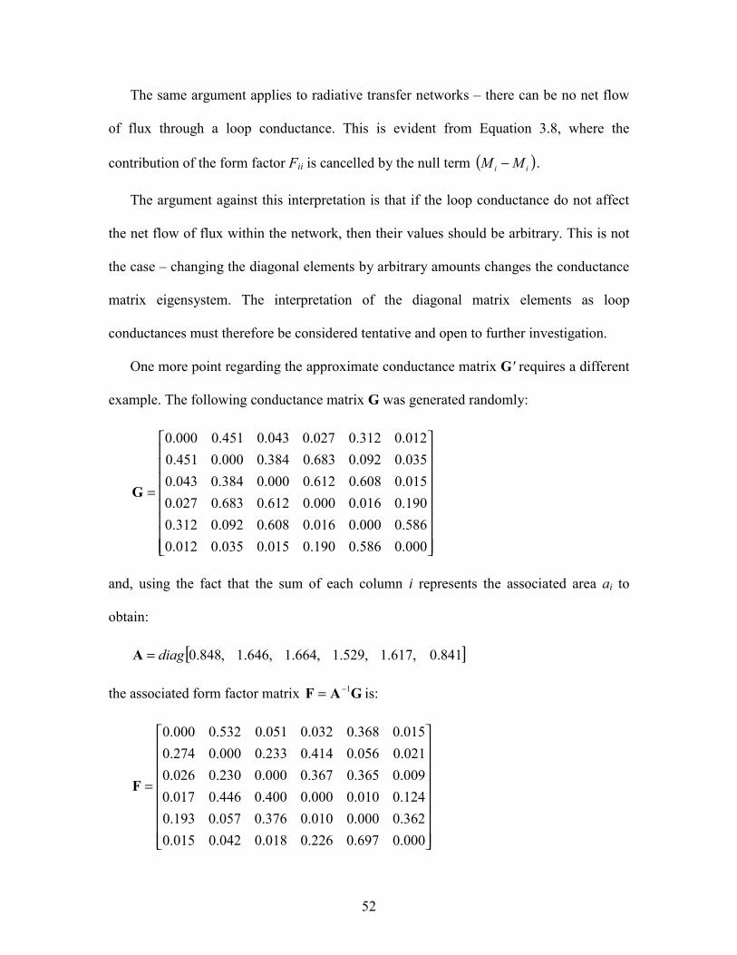
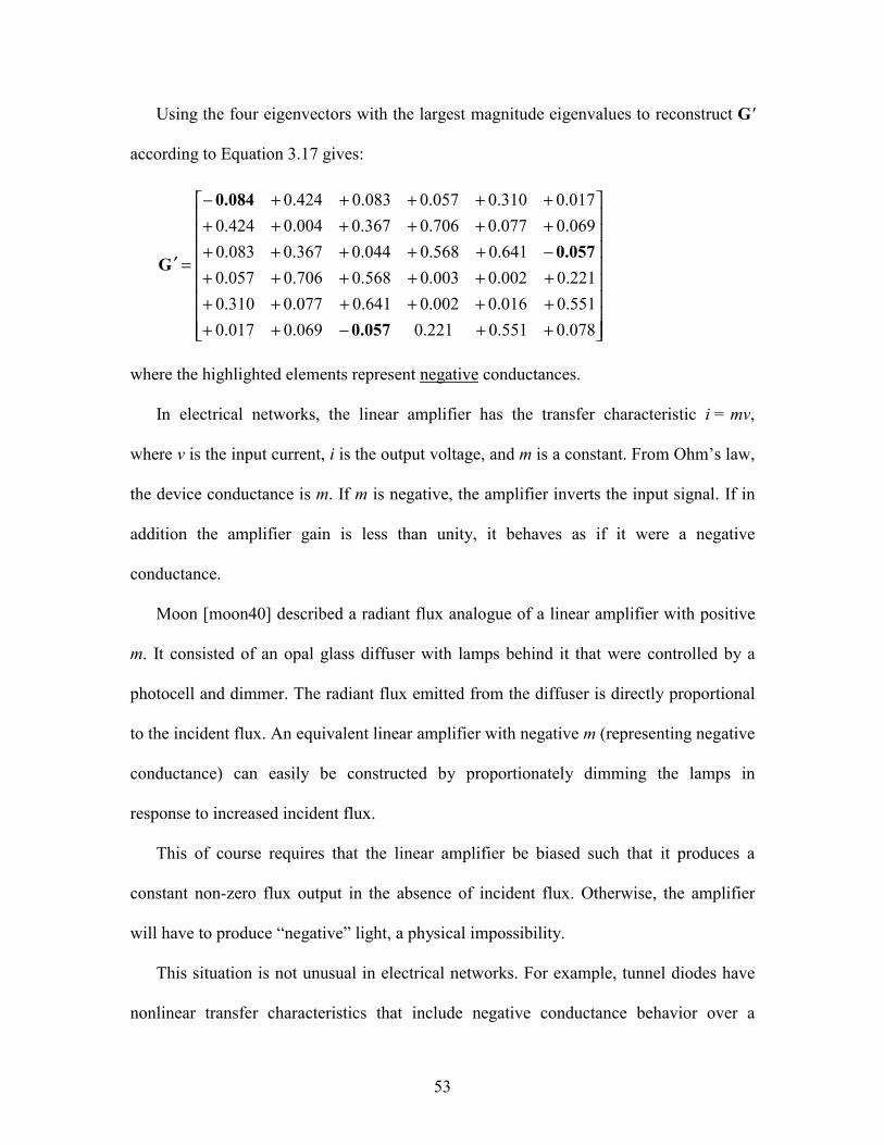
3.5 Approximate Conductance Networks
Applying the spectral theorem to the symmetric radiative transfer conductance matrix G,
we have:
∑=
ΤΤ ==n
iiii
1vvVDVG λ (3.18)
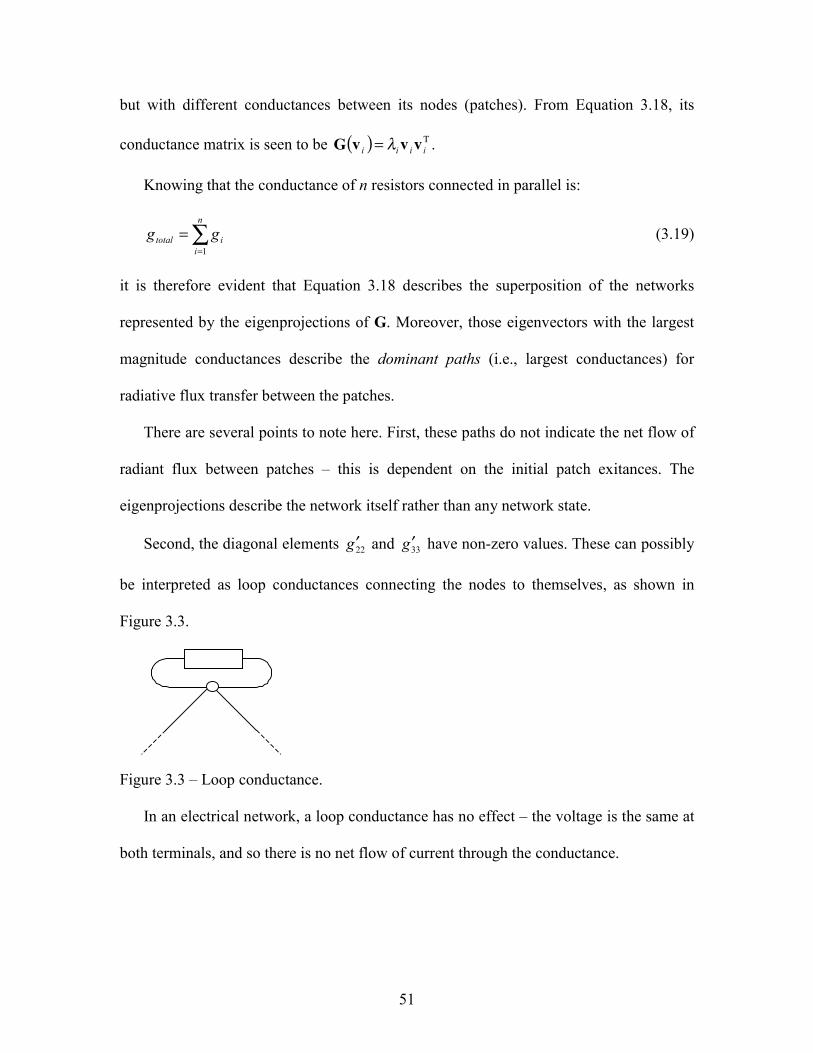
The question is whether this spectral decomposition of G has any physical meaning.
If it does, it may offer a useful approach to solving the radiosity equation.
49
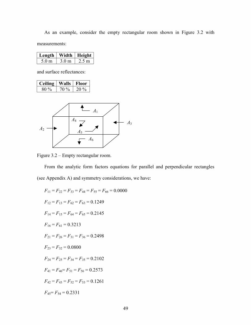
As an example, consider the empty rectangular room shown in Figure 3.2 with
measurements:
Length Width Height 5.0 m 3.0 m 2.5 m
and surface reflectances:
Ceiling Walls Floor 80 % 70 % 20 %
Figure 3.2 – Empty rectangular room.
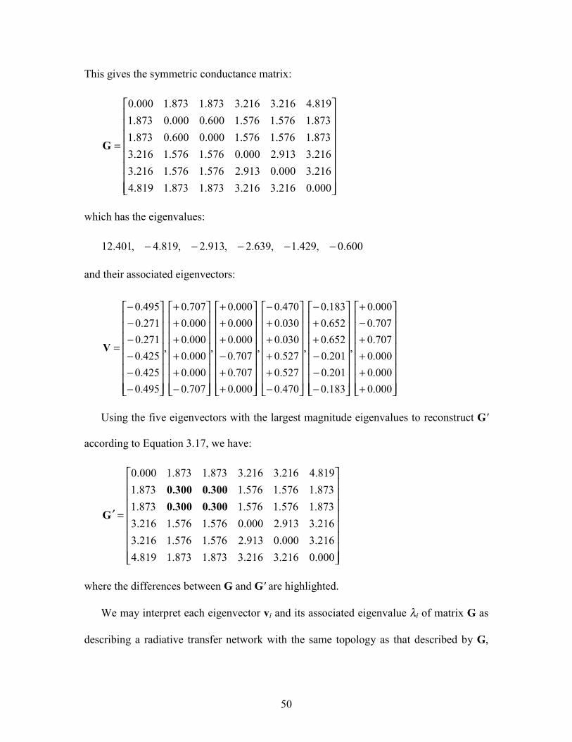
From the analytic form factors equations for parallel and perpendicular rectangles
(see Appendix A) and symmetry considerations, we have:
[shao93] M. Shao and N. Badler. 1993. “Analysis and Acceleration of Progressive
Refinement Radiosity Method,” Proceedings of the Fourth Eurographics
Workshop on Rendering, Paris, France, pp. 247–258.
[sieg92] R. Siegel and J. R. Howell. 1992. Thermal Radiation Heat Transfer, Third
Edition. Hemisphere Publishing, Washington, DC.
[sill94] F. X. Sillion and C. Puech. 1994. Radiosity & Global Illumination. Morgan
Kaufmann, San Francisco, CA.
[spar78] E. Sparrow and R. Cess. 1978. Radiation Heat Transfer. Hemisphere
Publishing, Washington, DC.
101
[thom94] R. E. Thomas and A. J. Rosa. 1994. The Analysis and Design of Linear
Circuits. Prentice-Hall, Englewood Cliffs, NJ.
[tsin98] N. Tsingos. 1998. Simulation de Champs Sonores de Haute Qualité pour des
Applications Graphiques Interactives. PhD thesis, Université Joseph Fourier,
Grenoble, France.
[unde75] R. Underwood. 1975. An Iterative Block Lanczos Method for the Solution of
Large Sparse Symmetric Eigenproblems. PhD thesis, Technical Report
STAN-CS-75-496, Stanford University, Stanford, CA.
[wilk65] J. H. Wilkinson. 1965. The Algebraic Eigenvalue Problem. Clarendon Press,
Oxford, UK.
[wilk71] J. H. Wilkinson and C. Reinsch. 1971. Handbook for Automatic Computation.
Berlin, Germany: Springer Verlag.
[wu98] K. Wu and H. Simon. 1998. Thick-Restart Lanczos Method for Symmetric
Eigenvalue Problems. Technical Report LBNL-41412, Lawrence Berkeley
National Laboratory/NERSC, Berkeley, CA.
[yama26] Z. Yamauti. 1926. “The Light Flux Distribution of a System of Interreflecting
Surfaces,” Journal of the Optical Society of America 13(5):561–571.
102
Appendix A
MATLAB Experiments
A.1 Does It Really Work?
While the numerical experiments presented in Chapter Five demonstrate the application
of eigenvector radiosity to practical illumination engineering problems, they do not
provide an unequivocal answer to the question: does eigenvector radiosity really work?
The problem is that the Helios progressive radiosity renderer used for the numerical
experiments calculates form factors using numerical quadrature rather than analytic
techniques. Moreover, these form factors model shooting patch as having differential
rather than a finite areas.
For most progressive radiosity applications these approximate form factors are
acceptable – the error is typically less than ±1 percent [ashd94]. However, it is advisable
to implement eigenvector radiosity using analytic form factors, if only to examine its
behavior with simple environments.
A.2 Form Factor Calculations
Despite their apparent simplicity, form factors are notoriously difficult to solve using
analytic methods. Johann Lambert, a pioneer researcher in photometry and likely the first
person to consider the problem, wrote [lamb60]:
Although this task appears very simple, its solution is considerably more knotted than
one would expect … the highly laborious computation would fill even the most patient
with disgust and drive them away.
103
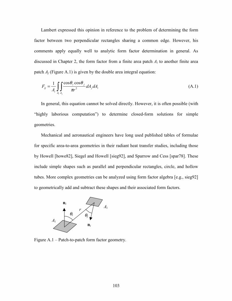
Lambert expressed this opinion in reference to the problem of determining the form
factor between two perpendicular rectangles sharing a common edge. However, his
comments apply equally well to analytic form factor determination in general. As
discussed in Chapter 2, the form factor from a finite area patch Ai to another finite area
patch Aj (Figure A.1) is given by the double area integral equation:
∫ ∫=i jA A
ijji
iij dAdA
rAF 2
coscos1π
θθ (A.1)
In general, this equation cannot be solved directly. However, it is often possible (with
“highly laborious computation”) to determine closed-form solutions for simple
geometries.
Mechanical and aeronautical engineers have long used published tables of formulae
for specific area-to-area geometries in their radiant heat transfer studies, including those
by Howell [howe82], Siegel and Howell [sieg92], and Sparrow and Cess [spar78]. These
include simple shapes such as parallel and perpendicular rectangles, circle, and hollow
tubes. More complex geometries can be analyzed using form factor algebra [e.g., sieg92]
to geometrically add and subtract these shapes and their associated form factors.
Figure A.1 – Patch-to-patch form factor geometry.
θj θi
Ai r
Ai ni
ni
104
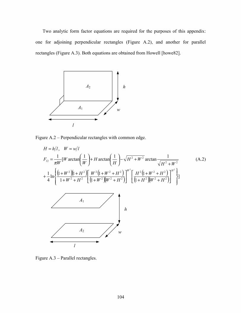
Two analytic form factor equations are required for the purposes of this appendix:
one for adjoining perpendicular rectangles (Figure A.2), and another for parallel
rectangles (Figure A.3). Both equations are obtained from Howell [howe82].
Figure A.2 – Perpendicular rectangles with common edge.
( )( ) ( )( )( )
( )( )( ) ]1
11
11
11ln41
1arctan1arctan1arctan[1,
22
222
222
222
222
22
22
22
2212
++++
++++
+++++
++−
+
=
==
HW
HWHHWH
HWWHWW
HWHW
WHWH
HH
WW
WF
lwWlhH
π (A.2)
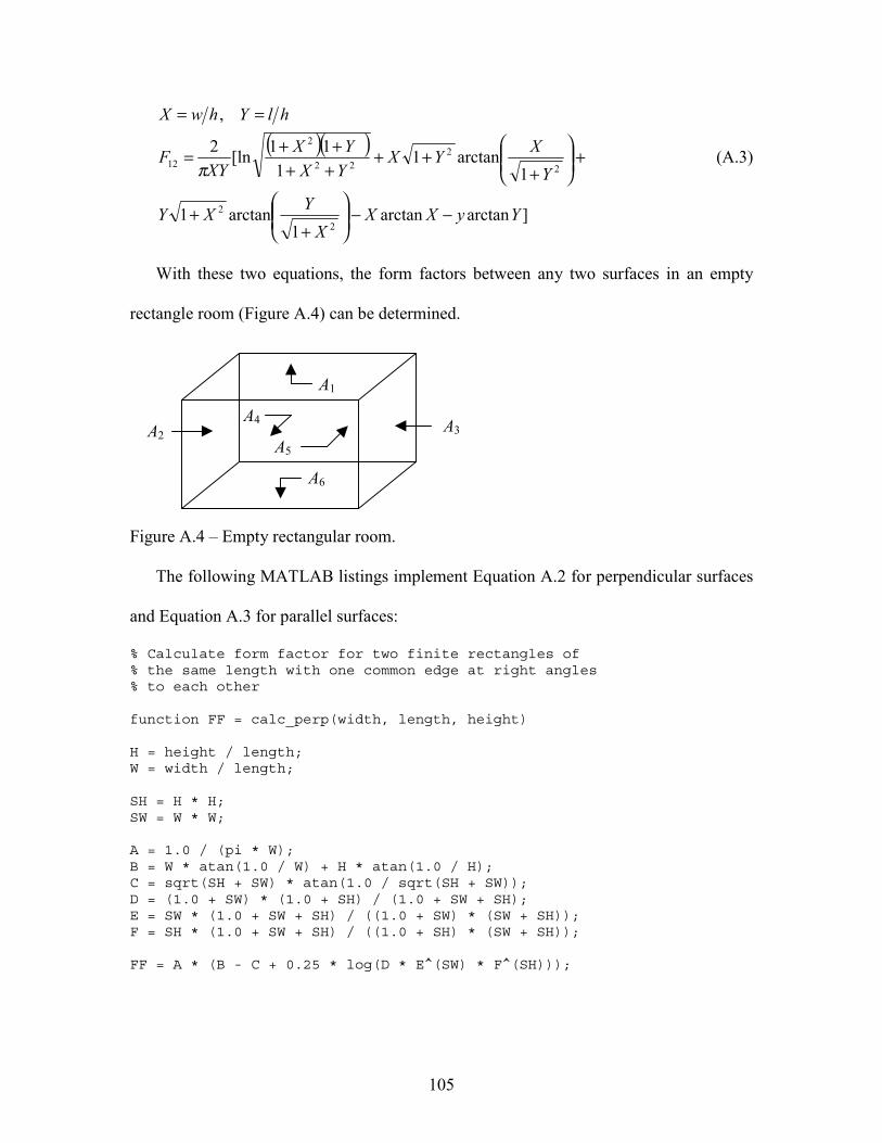
Figure A.3 – Parallel rectangles.
l
A2 w
h
A1
A1
A2
l
w
h
105
( )( )
]arctanarctan1
arctan1
1arctan1
111[ln2
,
2
2
2
222
2
12
YyXXX
YXY
YXYX
YXYX
XYF
hlYhwX
−−
++
+
+++
++++=
==
π (A.3)
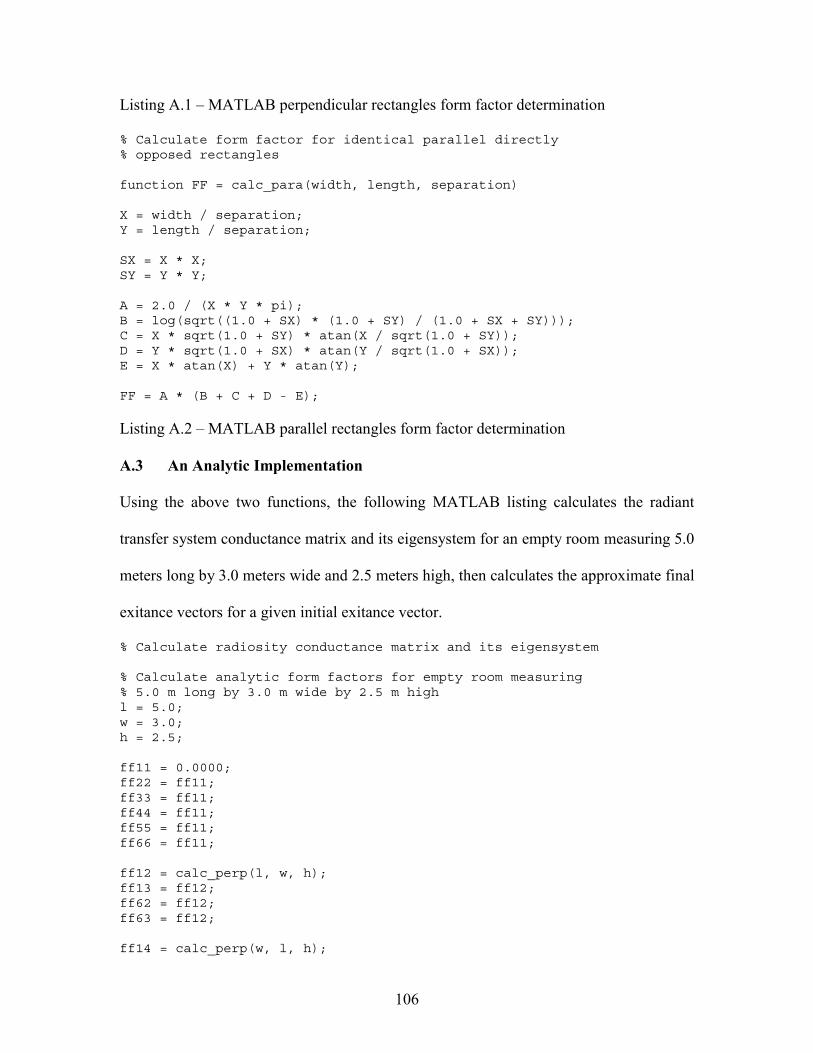
With these two equations, the form factors between any two surfaces in an empty
rectangle room (Figure A.4) can be determined.
Figure A.4 – Empty rectangular room.
The following MATLAB listings implement Equation A.2 for perpendicular surfaces
and Equation A.3 for parallel surfaces:
% Calculate form factor for two finite rectangles of % the same length with one common edge at right angles % to each other function FF = calc_perp(width, length, height) H = height / length; W = width / length; SH = H * H; SW = W * W; A = 1.0 / (pi * W); B = W * atan(1.0 / W) + H * atan(1.0 / H); C = sqrt(SH + SW) * atan(1.0 / sqrt(SH + SW)); D = (1.0 + SW) * (1.0 + SH) / (1.0 + SW + SH); E = SW * (1.0 + SW + SH) / ((1.0 + SW) * (SW + SH)); F = SH * (1.0 + SW + SH) / ((1.0 + SH) * (SW + SH)); FF = A * (B - C + 0.25 * log(D * E^(SW) * F^(SH)));
A3
A6
A1
A5 A2
A4
106
Listing A.1 – MATLAB perpendicular rectangles form factor determination
% Calculate form factor for identical parallel directly % opposed rectangles function FF = calc_para(width, length, separation) X = width / separation; Y = length / separation; SX = X * X; SY = Y * Y; A = 2.0 / (X * Y * pi); B = log(sqrt((1.0 + SX) * (1.0 + SY) / (1.0 + SX + SY))); C = X * sqrt(1.0 + SY) * atan(X / sqrt(1.0 + SY)); D = Y * sqrt(1.0 + SX) * atan(Y / sqrt(1.0 + SX)); E = X * atan(X) + Y * atan(Y); FF = A * (B + C + D - E);
Listing A.2 – MATLAB parallel rectangles form factor determination
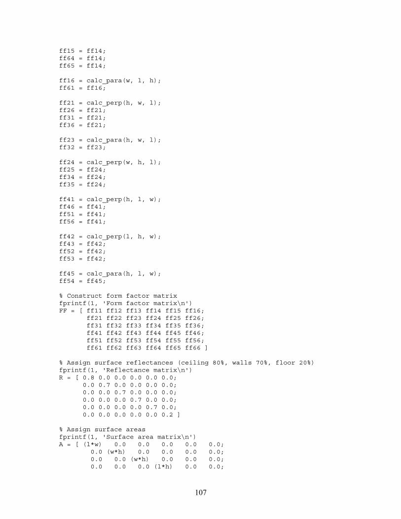
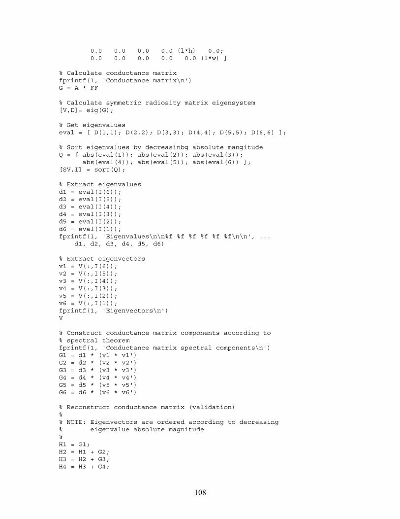
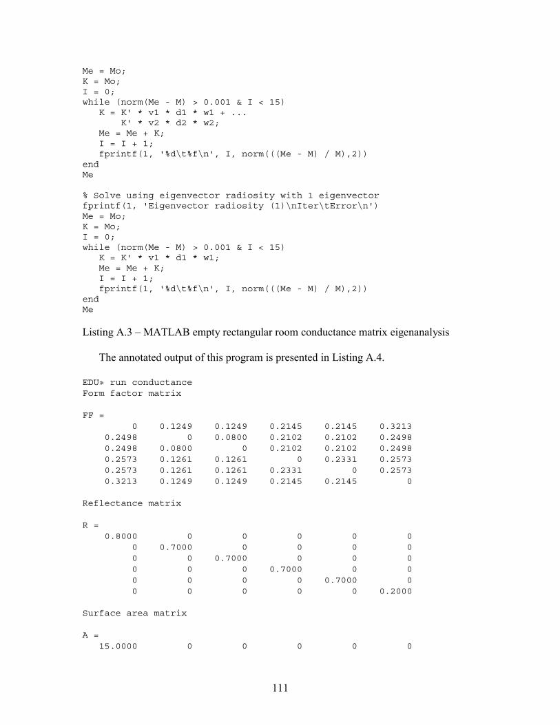
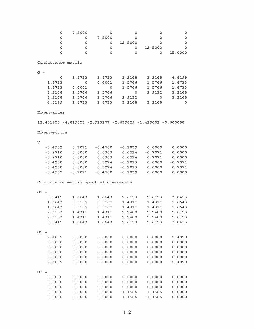
A.3 An Analytic Implementation
Using the above two functions, the following MATLAB listing calculates the radiant
transfer system conductance matrix and its eigensystem for an empty room measuring 5.0
meters long by 3.0 meters wide and 2.5 meters high, then calculates the approximate final
exitance vectors for a given initial exitance vector.
% Calculate radiosity conductance matrix and its eigensystem % Calculate analytic form factors for empty room measuring % 5.0 m long by 3.0 m wide by 2.5 m high l = 5.0; w = 3.0; h = 2.5; ff11 = 0.0000; ff22 = ff11; ff33 = ff11; ff44 = ff11; ff55 = ff11; ff66 = ff11; ff12 = calc_perp(l, w, h); ff13 = ff12; ff62 = ff12; ff63 = ff12; ff14 = calc_perp(w, l, h);
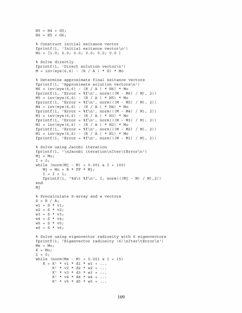
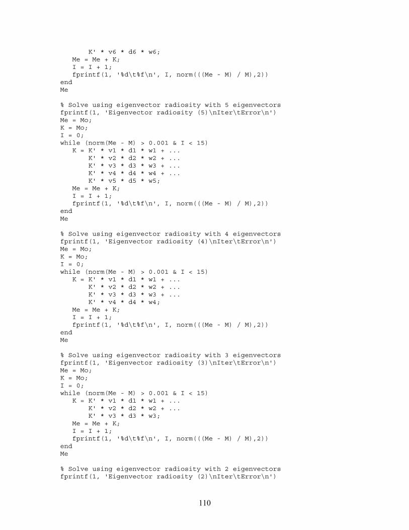
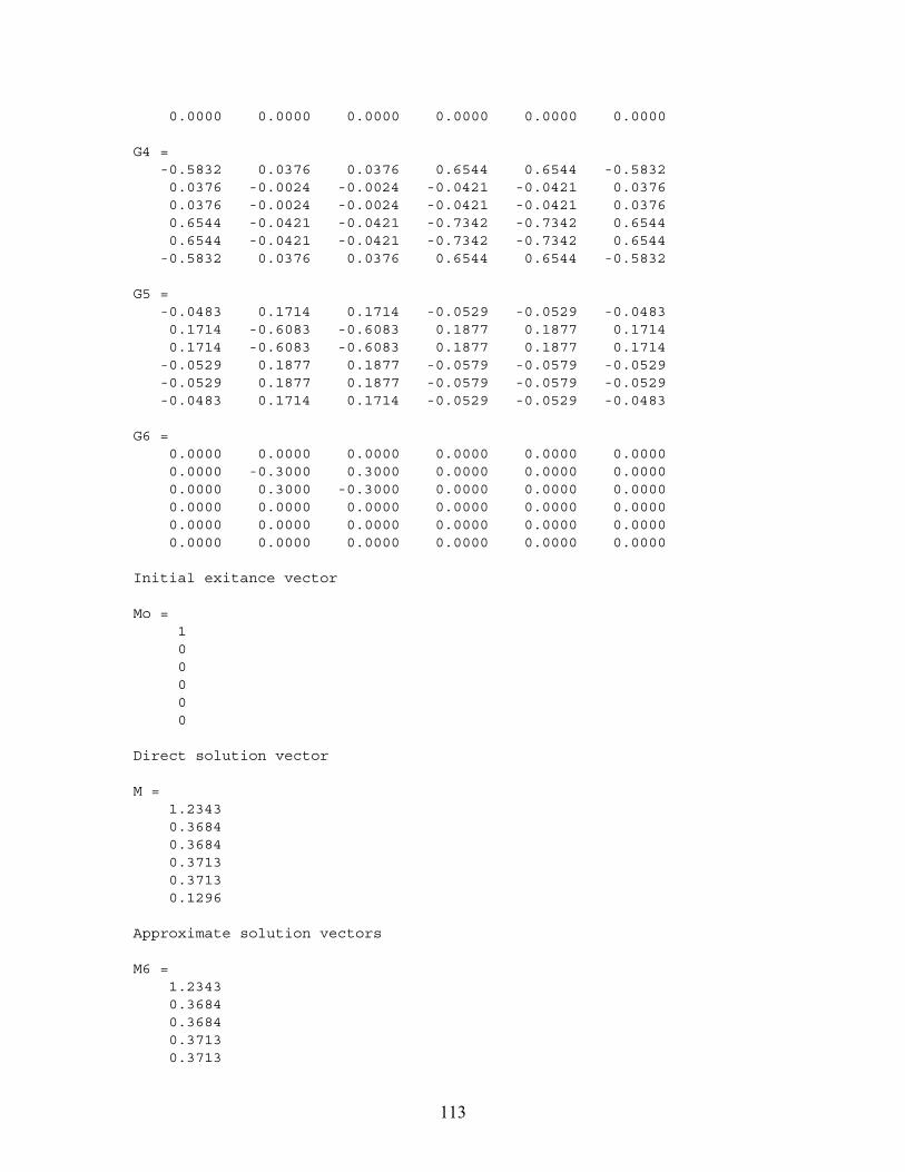
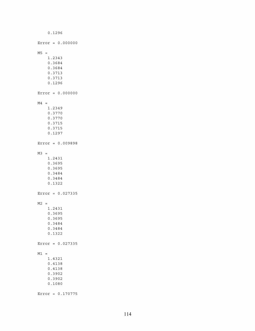
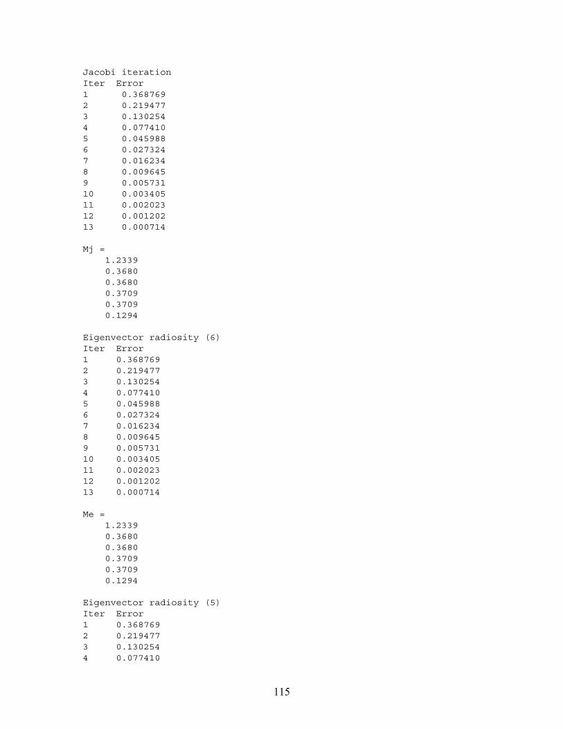
H5 = H4 + G5; H6 = H5 + G6; % Construct initial exitance vector fprintf(1, 'Initial exitance vector\n') Mo = [1.0; 0.0; 0.0; 0.0; 0.0; 0.0 ] % Solve directly fprintf(1, 'Direct solution vector\n') M = inv(eye(6,6) - (R / A ) * G) * Mo % Determine approximate final exitance vectors fprintf(1, 'Approximate solution vectors\n') M6 = inv(eye(6,6) - (R / A ) * H6) * Mo fprintf(1, 'Error = %f\n', norm(((M - M6) / M), 2)) M5 = inv(eye(6,6) - (R / A ) * H5) * Mo fprintf(1, 'Error = %f\n', norm(((M - M5) / M), 2)) M4 = inv(eye(6,6) - (R / A ) * H4) * Mo fprintf(1, 'Error = %f\n', norm(((M - M4) / M), 2)) M3 = inv(eye(6,6) - (R / A ) * H3) * Mo fprintf(1, 'Error = %f\n', norm(((M - M3) / M), 2)) M2 = inv(eye(6,6) - (R / A ) * H2) * Mo fprintf(1, 'Error = %f\n', norm(((M - M2) / M), 2)) M1 = inv(eye(6,6) - (R / A ) * H1) * Mo fprintf(1, 'Error = %f\n', norm(((M - M1) / M), 2)) % Solve using Jacobi iteration fprintf(1, '\nJacobi iteration\nIter\tError\n') Mj = Mo; I = 0; while (norm(Mj - M) > 0.001 & I < 100) Mj = Mo + R * FF * Mj; I = I + 1; fprintf(1, '%d\t %f\n', I, norm(((Mj - M) / M),2)) end Mj % Precalculate S-array and w vectors S = R / A; w1 = S * v1; w2 = S * v2; w3 = S * v3; w4 = S * v4; w5 = S * v5; w6 = S * v6; % Solve using eigenvector radiosity with 6 eigenvectors fprintf(1, 'Eigenvector radiosity (6)\nIter\tError\n') Me = Mo; K = Mo; I = 0; while (norm(Me - M) > 0.001 & I < 15) K = K' * v1 * d1 * w1 + ... K' * v2 * d2 * w2 + ... K' * v3 * d3 * w3 + ... K' * v4 * d4 * w4 + ... K' * v5 * d5 * w5 + ...
110
K' * v6 * d6 * w6; Me = Me + K; I = I + 1; fprintf(1, '%d\t%f\n', I, norm(((Me - M) / M),2)) end Me % Solve using eigenvector radiosity with 5 eigenvectors fprintf(1, 'Eigenvector radiosity (5)\nIter\tError\n') Me = Mo; K = Mo; I = 0; while (norm(Me - M) > 0.001 & I < 15) K = K' * v1 * d1 * w1 + ... K' * v2 * d2 * w2 + ... K' * v3 * d3 * w3 + ... K' * v4 * d4 * w4 + ... K' * v5 * d5 * w5; Me = Me + K; I = I + 1; fprintf(1, '%d\t%f\n', I, norm(((Me - M) / M),2)) end Me % Solve using eigenvector radiosity with 4 eigenvectors fprintf(1, 'Eigenvector radiosity (4)\nIter\tError\n') Me = Mo; K = Mo; I = 0; while (norm(Me - M) > 0.001 & I < 15) K = K' * v1 * d1 * w1 + ... K' * v2 * d2 * w2 + ... K' * v3 * d3 * w3 + ... K' * v4 * d4 * w4; Me = Me + K; I = I + 1; fprintf(1, '%d\t%f\n', I, norm(((Me - M) / M),2)) end Me % Solve using eigenvector radiosity with 3 eigenvectors fprintf(1, 'Eigenvector radiosity (3)\nIter\tError\n') Me = Mo; K = Mo; I = 0; while (norm(Me - M) > 0.001 & I < 15) K = K' * v1 * d1 * w1 + ... K' * v2 * d2 * w2 + ... K' * v3 * d3 * w3; Me = Me + K; I = I + 1; fprintf(1, '%d\t%f\n', I, norm(((Me - M) / M),2)) end Me % Solve using eigenvector radiosity with 2 eigenvectors fprintf(1, 'Eigenvector radiosity (2)\nIter\tError\n')
111
Me = Mo; K = Mo; I = 0; while (norm(Me - M) > 0.001 & I < 15) K = K' * v1 * d1 * w1 + ... K' * v2 * d2 * w2; Me = Me + K; I = I + 1; fprintf(1, '%d\t%f\n', I, norm(((Me - M) / M),2)) end Me % Solve using eigenvector radiosity with 1 eigenvector fprintf(1, 'Eigenvector radiosity (1)\nIter\tError\n') Me = Mo; K = Mo; I = 0; while (norm(Me - M) > 0.001 & I < 15) K = K' * v1 * d1 * w1; Me = Me + K; I = I + 1; fprintf(1, '%d\t%f\n', I, norm(((Me - M) / M),2)) end Me