HAL Id: hal-01075137https://hal.archives-ouvertes.fr/hal-01075137v2

Submitted on 2 Feb 2015

HAL is a multi-disciplinary open accessarchive for the deposit and dissemination of sci-entific research documents, whether they are pub-lished or not. The documents may come fromteaching and research institutions in France orabroad, or from public or private research centers.

L’archive ouverte pluridisciplinaire HAL, estdestinée au dépôt et à la diffusion de documentsscientifiques de niveau recherche, publiés ou non,émanant des établissements d’enseignement et derecherche français ou étrangers, des laboratoirespublics ou privés.

Distributed under a Creative Commons Attribution| 4.0 International License

Electromagnetic wave propagation and absorption inmagnetised plasmas: variational formulations and

domain decompositionAurore Back, Takashi Hattori, Simon Labrunie, Jean-Rodolphe Roche, Pierre

Bertrand

To cite this version:Aurore Back, Takashi Hattori, Simon Labrunie, Jean-Rodolphe Roche, Pierre Bertrand. Electromag-netic wave propagation and absorption in magnetised plasmas: variational formulations and domaindecomposition. ESAIM: Mathematical Modelling and Numerical Analysis, EDP Sciences, 2015, 49(5), pp.1239-1260. 10.1051/m2an/2015009. hal-01075137v2

Mathematical Modelling and Numerical Analysis Will be set by the publisher

Modelisation Mathematique et Analyse Numerique

ELECTROMAGNETIC WAVE PROPAGATION AND ABSORPTION IN

MAGNETISED PLASMAS: VARIATIONAL FORMULATIONS AND DOMAIN

DECOMPOSITION ∗

Aurore Back1, Takashi Hattori1, Simon Labrunie1, Jean-Rodolphe Roche1 and

Pierre Bertrand2

Abstract. We consider a model for the propagation and absorption of electromagnetic waves (inthe time-harmonic regime) in a magnetised plasma. We present a rigorous derivation of the modeland several boundary conditions modelling wave injection into the plasma. Then we propose severalvariational formulations, mixed and non-mixed, and prove their well-posedness thanks to a theoremby Sebelin et al. Finally, we propose a non-overlapping domain decomposition framework, show itswell-posedness and equivalence with the one-domain formulation. These results appear strongly linkedto the spectral properties of the plasma dielectric tensor.

Resume. Nous considerons un modele de propagation et d’absorption d’ondes electromagnetiques(en regime harmonique) dans un plasma magnetique. Nous presentons une justification rigoureusedu modele et diverses conditions aux limites modelisant l’injection de l’onde dans le plasma. Puisnous proposons plusieurs formulations variationnelles, mixtes ou non, et montrons qu’elles sont bienposees grace a un theoreme de Sebelin et al. Enfin, nous decrivons le principe d’une decompositionde domaine sans recouvrement, et etablissons le caractere bien pose de la formulation decomposeeet l’equivalence avec la formulation a un seul domaine. Ces resultats paraissent intimement lies auxproprietes spectrales du tenseur dielectrique du plasma.

1991 Mathematics Subject Classification. 35J57, 35Q60, 65N55.

January 28, 2015.

1. Introduction

Electromagnetic wave propagation in plasmas, especially magnetised ones, is an enormous subject [28]. Evenin a linear framework, the equations that describe it are generally highly anisotropic and, in many practicalsettings, highly inhomogeneous as well. The bewildering array of phenomena and parameters involved in this

Keywords and phrases: Magnetised plasma, Maxwell’s equations, domain decomposition.

∗ This work was supported by: the Agence Nationale de la Recherche (project “CHROME”) under contract ANR-12-BS01-0006-03; the Federation de Recherche Fusion par Confinement Magnetique–ITER; CNRS and INRIA.1 Universite de Lorraine, Institut Elie Cartan de Lorraine, UMR 7502, 54506 Vandœuvre-les-Nancy, France;CNRS, Institut Elie Cartan de Lorraine, UMR 7502, 54506 Vandœuvre-les-Nancy, France;e-mail: aurore.back,takashi.hattori,simon.labrunie,jean-rodolphe.roche@univ-lorraine.fr2 Universite de Lorraine, Institut Jean Lamour, UMR 7198, 54011 Nancy, France;CNRS, Institut Jean Lamour, UMR 7198, 54011 Nancy, France; e-mail: pierre.bertrand@univ-lorraine.fr

c© EDP Sciences, SMAI 1999

2 TITLE WILL BE SET BY THE PUBLISHER

modelling necessitates the derivation of simplified models tailored to the phenomenon under study, and to thetheoretical or computational purpose of this study.

Our interest lies in the numerical simulation of the propagation of electromagnetic waves near the so-calledlower hybrid frequency in a strongly magnetised plasma. Such waves are used in tokamak technology in orderto generate currents which stabilise or heat the plasma, thus bringing it closer to the conditions needed fornuclear fusion. The waves accelerate the charged particles that make up the plasma and transfer some oftheir energy to them through two main mechanisms: collisions between particles, which act as friction, andcollisionless Landau damping. This phenomenon, caused by a resonance between electromagnetic waves andparticles, is an efficient means of generating current in a magnetised plasma. Both mechanisms will be referredto as absorption. The basic physics of propagation and absorption is well understood [28]. Nevertheless, efficientand robust mathematical models have to be derived in order to do reliable numerical simulations in realisticsettings.

To perform these simulations, we have chosen to develop a finite element code which solves a suitable versionof the time-harmonic Maxwell equations in a strongly magnetised plasma. It is thus a full-wave code in theplasma community parlance, as opposed to ray-tracing codes which solve the equations of geometrical optics.Because of their simplicity, the latter have been more popular for many years; however, it turns out that formost parameter regimes of practical interest, geometrical optics fails to hold [7]. This has renewed the interestin full-wave simulations. A full-wave code based on spectral methods in cylindrical geometry has been developedby Peysson et al. [24]. Nevertheless, generalising to real tokamak configurations, with an arbitrary cross section,requires to use the more versatile finite element method.

On the other hand, full-wave computations in realistic settings are challenging because the lower hybridwavelength is very small compared to the machine size [31]. This led us to incorporate domain decompositioncapabilities in the code. This approach was preferred to, v.g., using state-of-the-art iterative methods to solvethe huge linear system arising from discretisation, as it is known [16] that iterative methods perform poorlywith strongly indefinite matrices such as those arising from time-harmonic equations. Thus, one has better splitthe computational domain into subdomains small enough to use a direct method. Another point in favour ofdomain decomposition is that the physical characteristics (such as density and temperature) typically vary overseveral orders of magnitude across a tokamak plasma. This might result in an extremely ill-conditioned linearsystem. However, this variation is normally continuous: another usual motivation of domain decomposition,viz., discontinuity in the equation coefficients, does not play any role here.

In this article, we will present the theoretical and mathematical foundations of our code: the derivation of thephysical model, a discussion of the possible variational formulations and their well-posedness, and the domaindecomposition framework. The code itself will be presented in a future publication, with a series of numericaltests. A preliminary version, without domain decomposition and differing in several respects, has been reportedin [23].

The outline of the article is as follows. In §2 we present a new, rigorous derivation of the model. We have feltthis necessary, as plasma physics textbooks (such as [28]) generally invoke spurious assumptions, which actuallyare not satisfied in real tokamak plasmas. They start by assuming that the external magnetic field and plasmacharacteristics are (at least approximately) homogeneous, and neglecting absorption phenomena. The latterare only discussed as an afterthought, if at all. We shall see that inhomogeneity is a non-issue, and absorptioncan be seamlessly integrated into the model. This is fortunate, as this phenomenon plays a crucial role in thewell-posedness of the variational formulations, with or without domain decomposition. Actually, a simplifiedmodel related to ours is known to be ill-posed in absence of absorption [14], which has an extremely importantconsequence: the global heating effect does not vanish as absorption tends to zero. If the limiting model werewell-posed, heating would be negligible when absorption is very small, as is the case in real tokamak plasmas.The section ends with a brief discussion of the boundary conditions that can model wave injection into theplasma.

TITLE WILL BE SET BY THE PUBLISHER 3

In §§3 and 4 we discuss the various possible variational formulations for the injection-propagation-absorptionmodel, and prove their well-posedness. The simplest one (which we call the plain formulation) has beendiscussed in [27]. We recall the results of this reference, which has not been published in a journal and thushas not reached a wide readership. Then, we show how they extend to mixed and augmented formulations inthe sense of [11]. Mixed formulations enforce the divergence condition on the electric field, and thus controlthe so-called “space charge” phenomena. Augmented formulations allow one to use the simpler nodal finiteelements [2–4, 11, 12, etc] instead of the edge (Nedelec) elements. Furthermore, the computed solution iscontinuous (like the physical solution), which avoids spurious difficulties when coupling with other solversof computational plasma physics. We conclude this part by listing a few properties of the functional spaces thatappear in the variational formulations.

In §5 we present the non-overlapping domain decomposition framework for our equations. Following theabove discussion, we focus on the mixed augmented formulation. We prove the well-posedness of the domain-decomposed formulation and its equivalence with the initial, one-domain formulation. This parallels and gen-eralises the work done in [4] for the time-dependent Maxwell equations in a homogeneous, isotropic, and non-absorbing medium. Notice, however, that our problem is considerably more difficult to solve numerically thanin the latter work: the matrix of the linear system arising from the discretisation of our variational formulationis neither definite nor Hermitian, unlike that of [4].

2. Electromagnetic waves: model problem

The physical system we are interested in is a plasma or totally ionised gas, pervaded by a strong, external,static magnetic field B0(x). (We shall always denote vector quantities by boldface letters.) Such a medium canbe described as a collection of charged particles (electrons and various species of ions) which move in vacuumand create electromagnetic fields which, in turn, affect their motion. Electromagnetic fields are, thus, governedby the usual Maxwell’s equations in vacuum:

curlE = −∂B∂t

, curlB = µ0 J +1

c2∂E

∂t; (1)

div E = /ε0, divB = 0. (2)

Here E and B denote the electric and magnetic fields; and J the electric charge and current densities; ε0and µ0 the electric permittivity and magnetic permeability of vacuum, with ε0 µ0 c

2 = 1.

2.1. Wave propagation equation

The electromagnetic field is the sum of a static part and a small perturbation caused by the penetration ofan electromagnetic wave. The latter is assumed to be time-harmonic. To simplify the discussion, we assumethe plasma to be in mechanical and electrostatic equilibrium in the absence of the wave. Thus, the electric andmagnetic fields can be written as

E(t,x) = ǫℜ[E(x)e−iωt] and B(t,x) = B0(x) + ǫℜ[B(x)e−iωt], (3)

where i =√−1, ℜ denotes the real part, ǫ≪ 1, and ω > 0 is the wave frequency. In the same way, we have

J (t,x) = ǫℜ[J(x)e−iωt] and (t,x) = ǫℜ[ρ(x)e−iωt]. (4)

The static parts of E, J , are zero by the equilibrium assumption. Furthermore, the static magnetic fieldsatisfies divB0 = 0 and curlB0 = 0, as its sources are supposed to be outside the plasma. Plugging this ansatzin the Maxwell equations (1), (2), we find:

curlE = iωB, curlB + iωc−2 E = µ0 J ; (5)

divE = ρ/ε0, divB = 0. (6)

4 TITLE WILL BE SET BY THE PUBLISHER

Eliminating the variable B between the two equations in (5), one finds

curl curlE − ω2

c2 E = iωµ0 J . (7)

We will shortly show that the medium obeys a linear, inhomogeneous and anisotropic Ohm law:

J(x) = σ(x)E(x). (8)

The expression of the conductivity tensor σ will be derived in the next section. Finally, Eq. (7) becomes

curl curlE − ω2

c2

(I +

i

ε0ωσ

)E = 0, (9)

where I is the identity matrix.

2.2. The plasma response tensor

As in [24, 26], the current density J in (8) appears as the sum of a “classical” part, which can be explainedby a fluid model, and a kinetic correction arising from Landau damping; both are linear in E. Let us begin withthe classical part. The particles species are labelled with the subscript ς ; the charge and mass of one particleare called qς and mς . In a first approach the plasma is assumed to be “cold”, i.e., the thermal agitation ofparticles, and thus their pressure, is negligible. Each species obeys the momentum conservation equation,1

mς∂uς

∂t+mς (uς · ∇)uς − qς (E + uς ×B) +mς νc uς = 0 (10)

where uς denotes the Eulerian fluid velocity and νc is the ion-electron collision frequency. (Collisions betweenparticles of the same species do not change their bulk velocity.) The fluid velocity and the particle densitynς(t,x) are linked to the electric charge and current densities by:

=∑

ς

ς :=∑

ς

qς nς , J =∑

ς

J ς :=∑

ς

qς nς uς .

Multiplying Eq. (10) by nς qς/mς , we find

∂J ς

∂t+

1

ς(J ς · ∇)J ς −

qςmς

(ς E +J ς ×B) + νc J ς = 0. (11)

Then, we use the ansatz (3)–(4). More specifically, for each species ς , we assume

J ς(t,x) = ǫℜ[Jς(x)e−iωt] and ς(t,x) = qς n

0ς (x) + ǫℜ[ρς(x)e−iωt].

The static part of J ς vanishes, as the plasma is at rest when ǫ = 0. At order 1 in ǫ, one can discard the term(J ς · ∇)J ς altogether; in ς E and J ς × B, only the terms in qς n

0ς E and J ς ×B0 survive. Furthermore, we

introduce the plasma and cyclotron frequencies for each species

ωpς :=

√n0ς q

2ς

ε0mς, ωcς :=

|qς |mς

|B0|, (12)

1It can be derived by integrating in velocity the Vlasov equation, see for instance [28].

TITLE WILL BE SET BY THE PUBLISHER 5

as well as δς = sign(qς) and the unit vector b = B0

|B0|. Thus we obtain the relationship:

i(ω + iνc)J ς + ε0ω2pς E + δςωcς J ς × b = 0. (13)

At each point x, one considers an orthonormal Stix frame [28] (e1(x), e2(x), e3(x) = b(x)). For any vectorfield v, one denotes v‖ = v3e3 and v⊥ = v1e1 + v2e2 the components of v(x) parallel and perpendicularto B0(x). Taking the cross product of (13) with b on the right, we have:

i(ω + iνc)Jς × b+ ε0ω2pς E × b− δςωcς J ς⊥ = 0, (14)

as there holds J⊥ = b× (J × b). Again, we take the cross product of (14) with b on the left:

i(ω + iνc)J ς⊥ + ε0ω2pςE⊥ + δςωcς J ς × b = 0,

which allows us to eliminate J ς × b in (14):

((ω + iνc)

2 − ω2cς

)J ς⊥ = i(ω + iνc) ε0ω

2pς E⊥ − δςωcς ε0ω

2pς E × b. (15)

The parallel current J ς‖ := (J ς · b) b is obtained by taking the dot product of (13) with b:

Jς‖ =iε0ω

2pς

ω + iνcE‖. (16)

Thus, the total current density J ς = J ς‖ + J ς⊥ of the species ς is given as:

J ς =iε0ω

2pς

ω + iνcE‖ +

i(ω + iνc)ε0ω2pς

(ω + iνc)2 − ω2cς

E⊥ − δς ε0ω2pςωcς

(ω + iνc)2 − ω2cς

E × b. (17)

Taking all species into account and setting α(x) := ω + iνc(x), we find the expression of the “classical”current density:

Jcla = iε0ω∑

ς

ω2pς

ωα︸ ︷︷ ︸

=:β

E‖ + iε0ωα

ω

∑

ς

ω2pς

α2 − ω2cς

︸ ︷︷ ︸=:γ

E⊥ − ε0ω1

ω

∑

ς

δς ωcςω2pς

α2 − ω2cς

︸ ︷︷ ︸=:δ

E × b. (18)

In the Stix frame, we have E = E1e1 +E2e2 +E3b, E‖ = E3b, E × b = E2e1 − E1e2. This gives the classicalpart of the conductivity tensor in (8):

σcla = iε0ω

γ −iδ 0iδ γ 00 0 β

. (19)

The classical dielectric tensor is thus:

ε := I +i

ε0ωσcla =

1− γ iδ 0−iδ 1− γ 00 0 1− β

:=

S −iD 0iD S 00 0 P

, (20)

6 TITLE WILL BE SET BY THE PUBLISHER

where the functions S, D and P are given by

S(x) := 1− α(x)

ω

∑

ς

ω2pς(x)

α2(x)− ω2cς(x)

, (21)

D(x) :=1

ω

∑

ς

δς ωcς(x)ω2pς(x)

α2(x)− ω2cς(x)

, (22)

P (x) := 1−∑

ς

ω2pς(x)

ωα(x). (23)

We proceed with the Landau damping part. As it appears [26], only electron Landau damping in the directionparallel to B0 plays a significant role. The “resonant” current generated by this effect is thus of the form:

J res(x) = γe(x)E‖(x). (24)

The coefficient γe is derived from a local linearisation of the Vlasov equation in the neighbourhood of thepoint x. Following the classical treatment by Landau [21], and assuming a Maxwellian distribution function atorder 0 in ǫ, one finds [26]:

γe = ε0ω

√π

2

ω2pe ω

k3‖

(me

kB Te

)3/2

exp

(− ω2me

2 k2‖ kB Te

), (25)

where Te is the electron temperature (the subscript e refers to electrons), kB the Boltzmann constant, and k‖is the component of the wave vector k parallel to B0.

Adding the two contributions, J = Jcla + J res, we find the expression in the Stix frame of the conductivitymatrix appearing in (8):

σ = σcla +

0 0 00 0 00 0 γe

.

In other words, the equation (9) which governs electromagnetic wave propagation and absorption in the plasmacan be rewritten as:

curl curlE − ω2

c2 KE = 0, (26)

with the plasma response tensor given by:

K(x) =

S(x) −iD(x) 0iD(x) S(x) 0

0 0 P (x)

︸ ︷︷ ︸ε(x)=classical dielectric tensor

+i

ε0ω

0 0 00 0 00 0 γe(x)

︸ ︷︷ ︸Landau term

. (27)

The tensor K(x) is not Hermitian as soon as νc or γe > 0.

2.3. The injection-propagation-absorption model

Let Ω be a bounded open domain in R3, which represents the plasma volume in the tokamak. From theprevious subsection, we know the propagation-absorption equation:

curl curlE − ω2

c2 KE = 0 in Ω. (28)

TITLE WILL BE SET BY THE PUBLISHER 7

The entries of the plasma response tensor K are given as functions of x ∈ Ω. The divergence equation

div(KE) = 0 in Ω, (29)

is a direct consequence of the previous one and may appear redundant. Nevertheless, it will play an all-importantrole in the derivation of the mixed and augmented variational formulations.

A= antenna

ΓC

B0

Ω

Γ

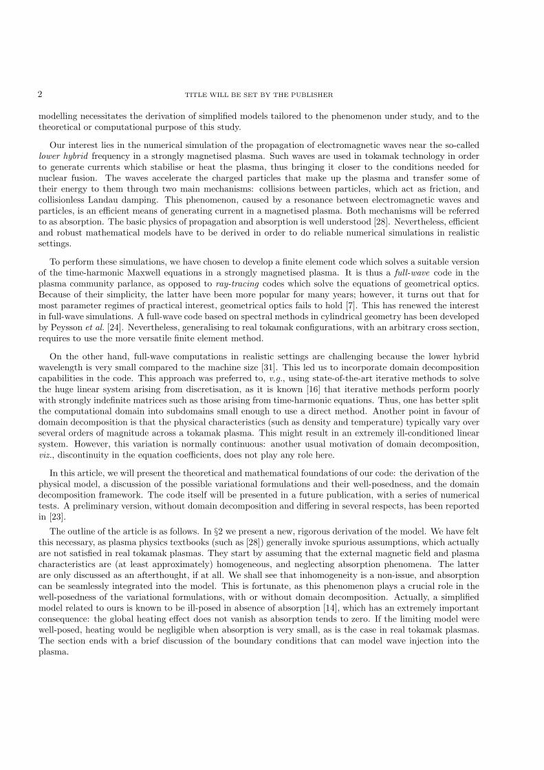
Figure 1. A cross-section of the domain Ω.

Furthermore, various boundary conditions may be considered. Let Γ be the boundary of Ω, and n theoutgoing unitary normal vector. This boundary is made up of two parts (see Figure 1): ΓA corresponds to theantenna and ΓC = Γ \ ΓA is the remainder. Introducing the surface current jA flowing through the antenna,the usual jump relations between media [6,20] give: B⊤ = −µ0 jA×n, where B⊤ denotes the component of Btangent to the boundary. Using the first part of (5), we deduce:

curlE × n = iωµ0 jA on ΓA. (30)

It appears as a Neumann (natural) condition. This modelling seems more relevant than that of [24,26,27], wherejA is treated as a ficticious volumic current in Ω. Alternatively, one can use an essential (Dirichlet) condition:

E × n = EA × n on ΓA, (31)

where EA is the electric field excited at the antenna. On the rest of the boundary, we use a perfectly conducting(homogeneous Dirichlet) boundary condition

E × n = 0 on ΓC , (32)

for the sake of simplicity.

3. Variational formulations

3.1. Functional setting

In the whole article, we suppose that the domain Ω is a curved polyhedron, i.e., a connected Lipschitz domainwith piecewise smooth boundary such that, near any point of its boundary, Ω is locally C∞-diffeomorphic to aneighbourhood of a boundary point of a polyhedron. This definition includes both smooth domains and straightpolyhedra. Furthermore, the boundaries ΓA, ΓC are collections of smooth faces separated by smooth edges,possibly meeting at vertices.

8 TITLE WILL BE SET BY THE PUBLISHER

We shall use boldface letters for the functional spaces of vector fields, v.g., L2(Ω) = L2(Ω)3. The innerproduct in L2(Ω) or L2(Ω) will be denoted (· | ·)Ω. Most unknowns and test functions are complex-valued, sothis inner product is Hermitian. “Duality” products 〈ϕ, v〉V will be linear in the first variable ϕ and anti-linearin the second v; the subscript V indicates the space to which the latter belongs. In this case, ϕ ∈ V ′, the spaceof anti-linear forms on V , which we call its dual for short. The subscripts Ω, V may be dropped when thecontext is clear.

Let H(curl; Ω) be the usual space of square integrable vector fields with square integrable curl in Ω. Weintroduce the ranges of the tangential trace mapping γ⊤ : v 7→ v × n and the tangential component mappingπ⊤ : v 7→ v⊤ := n× (v × n) from H(curl; Ω):

TT(Γ) := ϕ ∈ H−1/2(Γ) : ∃v ∈ H(curl; Ω), ϕ = v × n|Γ, (33)

TC(Γ) := λ ∈ H−1/2(Γ) : ∃v ∈ H(curl; Ω), λ = v⊤|Γ. (34)

These spaces have been described in [9], where they are respectively denoted H−1/2‖ (divΓ,Γ) = TT(Γ) and

H−1/2⊥ (curlΓ,Γ) = TC(Γ). Furthermore [10], they are in duality with respect to the pivot space L2

t (Γ) := w ∈L2(Γ) : w ·n = 0. This allows one to derive an integration by parts formula, valid for any u, v ∈ H(curl; Ω):

(u | curl v)Ω − (curlu | v)Ω = 〈u× n,v⊤〉TC(Γ) . (35)

Traces on a part of the boundary, v.g. ΓC , can be defined straightforwardly: the range spaces, calledH−1/2‖,00 (divΓC ,ΓC)

and H−1/2⊥,00 (curlΓC ,ΓC) in [9], will be denoted here TT(ΓC), TC(ΓC). Introducing the space

HC0 (curl; Ω) := u ∈ H(curl; Ω) : u× n|ΓC

= 0, (36)

i.e., the subspace of fields satisfying the essential condition (32), the range of the trace mappings on the rest ofthe boundary ΓA will be denoted

TT(ΓA) = ϕ ∈ H−1/2(ΓA) : ∃v ∈ HC0 (curl; Ω), ϕ = v × n|ΓA

, (37)

= ϕ ∈ TT(ΓA) : the extension of ϕ by 0 to Γ belongs to TT(Γ),TC(ΓA) = λ ∈ H−1/2(ΓA) : ∃v ∈ HC

0 (curl; Ω), λ = v⊤|ΓA (38)

= λ ∈ TC(ΓA) : the extension of λ by 0 to Γ belongs to TC(Γ),

instead of the “learned” notationsH−1/2‖ (div0ΓA

,ΓA) andH−1/2⊥ (curl0ΓA

,ΓA) of [9]. The spaces TT(ΓA) andTC(ΓA)

are in duality with respect to the pivot space L2t (ΓA), and similarly for TC(ΓA) and TT(ΓA).

Similarly, we introduce the Hilbert space:

H(divK; Ω) := u ∈ L2(Ω) : div(Ku) ∈ L2(Ω), (39)

endowed with its canonical norm. IfK ∈ L∞(Ω;M3(C)), it can be alternatively characterised asH(divK; Ω) :=u : Ku ∈ H(div; Ω), and the conormal trace Ku · n of a field u ∈ H(divK; Ω) is defined as an elementof H−1/2(Γ). Then we have another useful integration by parts formula, valid for all u ∈ H(divK; Ω) andϕ ∈ H1(Ω):

(div(Ku) | ϕ)Ω + (Ku | gradϕ)Ω = 〈Ku · n, ϕ〉H1/2(Γ) . (40)

If ϕ ∈ H10(Ω), the above formula can be extended to u ∈ L2(Ω). In that case, div(Ku) ∈ H−1(Ω) and

〈div(Ku), ϕ〉H1

0(Ω) + (Ku | gradϕ)Ω = 0. (41)

TITLE WILL BE SET BY THE PUBLISHER 9

In both cases, the scalar product (Ku | gradϕ)Ω can be written (u | K∗ gradϕ)Ω, with K∗ the conjugatetranspose of K.

3.2. Non-mixed formulations

Applying the Green formula (35) to (28) with the boundary conditions (30) and (32), the electric field appearsas solution to the following variational formulation: Find E ∈ HC

0 (curl; Ω) such that:

a(E,F ) = l(F ), ∀F ∈ HC0 (curl; Ω) (42)

where the forms a and l are:

a(u,v) := (curlu | curl v)Ω − ω2

c2 (Ku | v)Ω, (43)

l(v) := iωµ0〈jA,v⊤〉TC(ΓA). (44)

The formulation (42) will be called the plain formulation. It can be regularised by adding to both sides a termrelated to the divergence. To this end, we introduce the spaces:

X(K; Ω) := H(curl; Ω) ∩H(divK; Ω), (45)

XCN (K; Ω) := HC

0 (curl; Ω) ∩H(divK; Ω), (46)

endowed with their canonical norms and inner products. Using Eq. (29), we obtain the augmented variationalformulation: Find E ∈ XC

N (K; Ω) such that:

as(E,F ) = l(F ), ∀F ∈ XCN (K; Ω) (47)

with the augmented sesquilinear form as(·, ·) (s ∈ C) defined on X(K; Ω) as

as(u,v) := a(u,v) + s (div(Ku) | div(Kv))Ω. (48)

3.3. Mixed formulations

Alternatively, the divergence condition (29) can be considered as a constraint. Starting from the plainformulation (42), we introduce a Lagrangian multiplier p ∈ H1

0(Ω) to dualise this constraint (cf. (41)) and weobtain a mixed unaugmented formulation which writes: Find (E, p) ∈ HC

0 (curl; Ω)×H10(Ω) such that

a(E,F ) + β(F , p) = l(F ), ∀F ∈ HC0 (curl; Ω), (49)

β(E, q) = 0, ∀q ∈ H10(Ω), (50)

where the form β is defined on L2(Ω)×H1(Ω) as:

β(v, q) := −(Kv | grad q)Ω. (51)

If we start from the augmented formulation (47) instead, we introduce a Lagrangian multiplier p ∈ L2(Ω)and arrive at the mixed augmented variational formulation: Find (E, p) ∈ XC

N (K; Ω)× L2(Ω) such that

as(E,F ) + b(F , p) = l(F ), ∀F ∈ XCN (K; Ω), (52)

b(E, q) = 0, ∀q ∈ L2(Ω), (53)

with b(·, ·) defined on H(divK; Ω)× L2(Ω) as:

b(v, q) := (div(Kv) | q)Ω. (54)

10 TITLE WILL BE SET BY THE PUBLISHER

3.4. Essential boundary conditions

The variational formulations for the essential conditions (31) and (32) are obtained in a similar way. Using testfields satisfying F ×n = 0 on ∂Ω in the Green formula (35), one derives the plain and augmented formulations:Find E ∈ HC

0 (curl; Ω), satisfying (31), and such that

a(E,F ) = 0, ∀F ∈ H0(curl; Ω) ; (55)

Find E ∈ XCN (K; Ω), satisfying (31), and such that

as(E,F ) = 0, ∀F ∈ XN (K; Ω), (56)

where we have set:

XN (K; Ω) := H0(curl; Ω) ∩H(divK; Ω). (57)

To analyse these formulations, one splits the electric field as E = EA+E, where EA is a lifting of the boundarydata and E satisfies the perfectly conducting condition on the whole boundary. Thus, one has to assume at

least that EA ∈ TC(ΓA). This is obviously sufficient for the unaugmented formulations. For the augmentedformulations, it is necessary to have a lifting in X(K; Ω). As we shall see in Remark 4.12 the existence of sucha lifting does not entail any supplementary condition on EA. In this case, E belongs to the space XN (K; Ω).The plain and augmented formulations satisfied by E are respectively:Find E ∈ H0(curl; Ω) such that

a(E,F ) = 〈f ,F 〉H0(curl;Ω) := −a(EA,F ), ∀F ∈ H0(curl; Ω) ; (58)

Find E ∈ XN (K; Ω) such that

as(E,F ) = Ls(F ), ∀F ∈ XN (K; Ω). (59)

The mixed augmented formulations satisfied by E and E write:Find (E, p) ∈ XC

N (K; Ω)× L2(Ω), with E satisfying (31), and such that

as(E,F ) + b(F , p) = 0, ∀F ∈ XN (K; Ω), (60)

b(E, q) = 0, ∀q ∈ L2(Ω). (61)

Find (E, p) ∈ XN (K; Ω)× L2(Ω) such that

as(E,F ) + b(F , p) = Ls(F ), ∀F ∈ XN (K; Ω), (62)

b(E, q) = ℓ(q), ∀q ∈ L2(Ω). (63)

The right-hand sides are given by:

Ls(v) := −a(EA,v)− s (div(KEA) | div(Kv))Ω := 〈f ,v〉+ s (g | div(Kv))Ω ; (64)

ℓ(q) := −(div(KEA) | q)Ω := (g | q)Ω . (65)

The reader may write the mixed unaugmented formulations as an exercise.

As usual when dealing with non-homogeneous essential conditions, we shall use the formulations in E,Eqs. (58), (59), and (62)–(63) to prove well-posedness. However, in practice, we discretise the formulationsin E, Eqs. (55), (56), and (60)–(61): both conditions (31) and (32) are handled by a pseudo-eliminationprocedure following a local change of basis [18].

TITLE WILL BE SET BY THE PUBLISHER 11

4. Well-posedness of the problem

In this section, we summarise the results of [27] — which deals with the plain formulation when γe = 0 —and show how they extend to our various formulations. We shall make the following assumption throughoutthe article.

Hypothesis 1. The real functions νc, ωcς and ωpς , for each species ς (ions and electrons) are bounded aboveand below by strictly positive constants on Ω. The function γe is non-negative and bounded above.

Remark 4.1. The collision frequency νc is given by the following expression [17], where Z is the ion chargenumber (i.e., their charge is equal to Z |qe|):

νc =

√2

π

ωpe ln Λ

Λ, with: Λ =

12π

Zne

(ε0 kB Tene q2e

)3/2

. (66)

A plasma is characterised by Λ ≫ 1. In this framework, and recalling the expressions (12) of ωcς , ωpς and (25)of γe, one checks that Hypothesis 1 is satisfied provided the densities nς and the electron temperature Te arebounded above and below by strictly positive constants on Ω. This is the case in all practical settings.

4.1. Spectral properties of the plasma response tensor

It is not difficult to check that the eigenvalues of the matrix K are

λ1 = S +D, λ2 = S −D, λ3 = P +i

ε0ωγe.

Furthermore, K is a normal matrix (K∗ K = KK∗), and its singular values are the moduli of its eigenvalues.Then, one deduces from (21)–(23) the expression of the imaginary parts (ℑλi)i=1...3:

ℑλ1(x) =νc(x)

ω

∑

ς

ω2pς(x)

(ω2cς(x)− ω2 + ν2c (x))

2 + 4ω2ν2c (x)

[(ω − δς ωcς(x))

2 + ν2c (x)],

ℑλ2(x) =νc(x)

ω

∑

ς

ω2pς(x)

(ω2cς(x)− ω2 + ν2c (x))

2 + 4ω2ν2c (x)

[(ω + δς ωcς(x))

2 + ν2c (x)],

ℑλ3(x) =νc(x)

ω(ω2 + ν2c (x))

∑

ς

ω2pς(x) +

1

ε0ωγe(x).

From the above calculations, one easily infers a fundamental bound.

Lemma 4.2. Under Hypothesis 1, there exist two constants η ≥ ζ > 0, dependent on ω, such that

η(z∗z) ≥ |z∗K(x)z| ≥ ℑ[(z∗K(x)z)] ≥ ζ(z∗z), ∀z ∈ C3, ∀x ∈ Ω. (67)

Remark 4.3. When the ωcς and ωpς , νc and γe have typical values for tokamak plasmas, and ω is of theorder of the lower hybrid frequency, one has ℜλ1 ≥ 0, while ℜλ2 ≤ 0 and ℜλ3 ≤ 0. No lower bound holds for|ℜ[(z∗K(x)z)]|.

4.2. Coercivity and inf-sup condition

We recall the fundamental result of Sebelin et al. [27].

Theorem 4.4. Let V and H be Hilbert spaces such that the embedding V → H is continuous. Let a(·, ·) be asesquilinear form on V × V . If there exists three strictly positive constants α, λ, γ such that:

12 TITLE WILL BE SET BY THE PUBLISHER

(1) the real part of a(·, ·) is Garding-elliptic on V , i.e.:

|ℜ[a(v, v)]| ≥ α‖v‖2V − λ‖v‖2H , ∀v ∈ V (68)

(2) the imaginary part of a(·, ·) is H-coercive, i.e.:

|ℑ[a(v, v)]| ≥ γ‖v‖2H , ∀v ∈ V, (69)

then the sesquilinear form a is V -elliptic.

Combined with Lemma 4.2, this theorem shows the well-posedness of the non-mixed formulations, by Lax–Milgram’s lemma.

Theorem 4.5. There exists a unique solution to the plain formulations (42) and (58), hence to (55). Thesame holds for the augmented formulations (47) and (59) — and thus for (56) — provided ℜs > 0 and ℑs ≤ 0.

Proof. As in [27], one uses Eq. (67) to check that the form a given by (43) is continuous on V = H(curl; Ω) andsatisfies the assumptions of Theorem 4.4 with H = L2(Ω). Thus, it is coercive (and continuous) on H(curl; Ω),a fortiori on the closed subspaces H0(curl; Ω) and HC

0 (curl; Ω). When ℜs > 0 and ℑs ≤ 0, the same appliesto the form as given by (48) on V = X(K; Ω). This form is coercive and continuous on the closed subspacesof X(K; Ω), v.g., XN (K; Ω) and XC

N (K; Ω).

To prove the well-posedness of mixed formulations, we have to check an inf-sup condition. This can be doneby following the lines of [11, 12].

Proposition 4.6. The sesquilinear form β defined by (51) satisfies an inf-sup condition on H0(curl; Ω)×H10(Ω),

i.e.there exists Cβ > 0 such that

∀q ∈ H10(Ω), sup

v∈H0(curl;Ω)

|β(v, q)|‖v‖H(curl)

≥ Cβ ‖q‖H1 . (70)

Proof. Fix q ∈ H10(Ω) and set v = grad q ∈ H0(curl; Ω). Lemma 4.2 shows that

|β(v, q)| = |(Kv | grad q)| = |(Kv | v)| ≥ ζ‖v‖2L2 = ζ‖v‖L2‖ grad q‖L2 .

On the other hand, ‖v‖H(curl) =(‖v‖2

L2 + ‖ curl v‖2L2

)1/2= ‖v‖L2 , and ‖ grad q‖L2 ≥ C ‖q‖H1 by Poincare’s

inequality. Hence the conclusion.

To proceed to the mixed augmented case, we state and prove a useful lemma.

Lemma 4.7. For any f ∈ H−1(Ω), the elliptic problem: Find φ ∈ H10(Ω) such that

−∆Kφ := − div(K gradφ) = f (71)

admits a unique solution, which satisfies |ψ|H1 ≤ C ‖f‖H−1 for some constant C.

Proof. Using (41) with u = grad φ, the variational formulation of (71) writes:

a(φ, ψ) := (K grad φ | gradψ)Ω = 〈f, ψ〉H1

0(Ω), ∀ψ ∈ H1

0(Ω). (72)

By Eq. (67), the form a satisfies

η |ψ|2H1(Ω) ≥ |a(ψ, ψ)| ≥ ζ |ψ|2H1(Ω), ∀ψ ∈ H10(Ω),

i.e., it is continuous and coercive on H10(Ω), and the formulation is well-posed by Lax–Milgram’s lemma.

TITLE WILL BE SET BY THE PUBLISHER 13

Remark 4.8. Elliptic problems with the operator ∆K∗ are also well-posed.

Proposition 4.9. The sesquilinear form b defined by (54) satisfies an inf-sup condition on XN (K; Ω)×L2(Ω),i.e.there exists Cb > 0 such that

∀q ∈ L2(Ω), supv∈XN (K;Ω)

|b(v, q)|‖v‖X

≥ Cb ‖q‖L2 . (73)

Proof. Fix q ∈ L2(Ω). According to Lemma 4.7, there exists φ ∈ H10(Ω) such that ∆Kφ = q. Setting v = gradφ,

we have v ∈ H0(curl; Ω) and div(Kv) = q, hence v ∈ H(divK; Ω) and finally v ∈ XN (K; Ω). It is boundedas:

‖v‖2X = ‖v‖2L2 + ‖ curl v‖2

L2 + ‖ divKv‖2L2

= ‖ gradφ‖2L2 + 0 + ‖ divK gradφ‖2L2

= |φ|2H1 + ‖q‖2L2 ≤ (1 + C2)‖q‖2L2 ,

On the other hand|b(v, q)| = |(divKv | q)| = |(q | q)| = ‖q‖2L2 .

Finally|b(v, q)|‖v‖X

≥ 1√1 + C2

‖q‖L2 ,

which we had to prove.

Theorem 4.10. There exists a unique solution to the mixed unaugmented formulation (49)–(50), and to itscounterpart for the Dirichlet boundary condition. The same holds for the mixed augmented formulations (52)–(53) and (62)–(63), provided ℜs > 0 and ℑs ≤ 0. Thus, the problem (60)–(61) is well-posed in this case.

Proof. The forms a and as are coercive, in particular, on the kernels of the forms β and b. The form b isobviously continuous, and so is β(·, ·) thanks to the boundedness of the entries of K. The inf-sup conditions(70) and (73) are exactly those needed for the Dirichlet formulations. In the Neumann case, they remain validwhen replacing H0(curl; Ω) with HC

0 (curl; Ω) or XN (K; Ω) with XCN (K; Ω), as the supremum is greater on

the bigger space. We conclude by the Babuska–Brezzi theorem.

To conclude this subsection, we observe that all formulations are equivalent to one another. For instance,the unique solution to the plain formulation satisfies (28) in D

′(Ω), hence divKE = 0 and E ∈ XCN (K; Ω) is

solution to the augmented formulation. Similarly, (E, 0) is solution to both mixed formulations, thus it coincideswith their respective unique solutions.

4.3. Miscellaneous properties

Here we collect and discuss some useful properties of our functional spaces. First, one has a Helmholtzdecomposition of vector fields into gradient and “K-solenoidal” parts.

Lemma 4.11. For any u ∈ L2(Ω) there exists a unique pair (φ,uT ) ∈ H10(Ω)×L2(Ω) satisfying the conditions

u = gradφ+ uT , div(KuT ) = 0 ; (74)

‖ gradφ‖L2 ≤ C‖u‖L2 , ‖uT ‖L2 ≤ C‖u‖L2 . (75)

Proof. If a solution exists, then ∆Kφ = div(Ku); the latter function belongs to H−1(Ω) under Hypothesis 1,with ‖ div(Ku)‖H−1 ≤ C ‖u‖L2 . Lemma 4.7 shows the existence and uniqueness of φ and uT = u− gradφ, aswell as the bounds (75).

Remark 4.12. Obviously, gradφ ∈ H0(curl; Ω) and uT ∈ H(divK; Ω). As particular cases:

14 TITLE WILL BE SET BY THE PUBLISHER

(1) If u ∈ H(curl; Ω), then uT ∈ H(curl; Ω) and thus uT ∈ X(K; Ω). Furthermore, uT × n = u × n:the ranges of the mappings γ⊤ and π⊤ from X(K; Ω) are identical to the ranges from H(curl; Ω), i.e.,TT(Γ) and TC(Γ).

(2) If u ∈ X(K; Ω), then gradφ ∈ XN (K; Ω), and the decomposition (74) is continuous in X norm.(3) As a consequence of the two previous points, both uT and gradφ belong to XN (K; Ω) if u does.

Remark 4.13. Thanks to Remark 4.8, one also has a decomposition into K∗-gradient and solenoidal parts:for any u ∈ L2(Ω), there is a unique pair (φ,uT ) ∈ H1

0(Ω)× L2(Ω) such that

u = K∗ gradφ+ uT and divuT = 0. (76)

The above results allow one to prove two powerful theorems on the space XN (K; Ω). They parallel thewell-known results valid for scalar or Hermitian positive definite dielectric tensors. The proofs are similar tothese classical cases and can be found in [18], so we will not detail them here.

Theorem 4.14. If Ω is Lipschitz, the space XN (K; Ω) is compactly embedded into L2(Ω).

Proof. Follow the lines of Weber [30], using Lemmas 4.2, 4.7 and 4.11.

Remark 4.15. If νc = γe = 0, the proof breaks down: without absorption, one cannot establish a Fredholmalternative for the model of §2.3 with Dirichlet boundary conditions, see also Remark 4.3. With Neumannboundary conditions, the embedding XC

N (K; Ω) → L2(Ω) is not compact when ΓA 6= ∅, whatever the matrixfield K. Thus, all usual strategies for proving well-posedness fail in the absence of absorption. Actually, thereis every reason to believe that the model is ill-posed in this case (see §1).Theorem 4.16. Assume that Ω has a C1,1 boundary, and that the functions νc, γe, ωcς and ωpς (for each

species ς) belong to C1(Ω). The space XN (K; Ω) is algebraically and topologically included in H1(Ω).

Proof. Following the lines of Birman–Solomyak [5], one shows that any u ∈ XN (K; Ω) admits a decomposition

u = uBS + gradϕ, with: uBS ∈ H10(Ω), ϕ ∈ H1

0(Ω), ∆Kϕ ∈ L2(Ω).

The usual elliptic theory [19], valid for the operator −∆−iK thanks to Lemma 4.2, shows that ϕ ∈ H2(Ω), giventhe smoothness of Ω and K. Hence u ∈ H1(Ω).

In other words, there holds XN (K; Ω) ⊂ H1N(Ω) := w ∈ H1(Ω) : w × n|Γ = 0; the converse inclusion

is obvious as K ∈ C1(Ω;M3(C)). Furthermore the embedding H1N(Ω) → XN (K; Ω) is continuous; thus the

converse embedding XN (K; Ω) → H1N(Ω) is continuous by the open mapping theorem.

Remark 4.17. Under the hypotheses of the above theorem, it is thus possible to discretise straightforwardlythe augmented and mixed augmented variational formulations of §3 with nodal (Lagrange or Taylor–Hood)finite elements. Note that this does not apply when the boundary is not smooth and has re-entrant corners,due to the singularity of the solution [13].

5. Non-overlapping domain decomposition framework

For the sake of simplicity, we assume from now essential boundary conditions, and we consider (cf. §3.4) thefollowing model problem:

curl curlE − ω2

c2 KE = f in Ω, (77)

div(KE) = g in Ω, (78)

E × n = 0 on Γ, (79)

TITLE WILL BE SET BY THE PUBLISHER 15

where the data (f , g) satisfy the compatibility condition div f = −ω2

c2 g. The mixed augmented variationalformulation reads:Find (E, p) ∈ XN (K; Ω)× L2(Ω) such that

as(E,F ) + b(F , p) = Ls(F ) := (f | F )Ω + s (g | div(KF ))Ω , ∀F ∈ XN (K; Ω), (80)

b(E, q) = ℓ(q) := (g | q)Ω, ∀q ∈ L2(Ω). (81)

As shown by the above notations, we have assumed f ∈ L2(Ω) and g ∈ L2(Ω). According to §4, this problemadmits a unique solution (E, p) ∈ XN (K; Ω)× L2(Ω), with p = 0.

5.1. Strong formulation

We introduce a non-overlapping domain decomposition [1, 22, 25]:

Ω =

Nd⋃

i=1

Ωi ; Ωi ⊂ Ω, i = 1, . . . , Nd ; Ωi ∩Ωj = ∅ if i 6= j. (82)

The exterior boundaries of subdomains are denoted Γi = Γ ∩ ∂Ωi, i = 1, . . . , Nd, and the interfaces betweenthem Σi,j = ∂Ωi ∩ ∂Ωj . We shall write i j whenever Σi,j is a non-empty topological surface, i.e., it has anon-zero area. To keep things simple, we assume that the Γi and Σi,j are smooth when they are topologicalsurfaces, and then that the Γi ∩ Σi,j and Σi,j ∩ Σi,k are smooth curves. This is generally achieved in practice.However, the skeleton of interfaces Σ =

⋃i,j Σi,j is not smooth, as there generally are (curved) dihedral angles

between interfaces.

The principle of domain decomposition for Maxwell’s equations has been known for some time, both in thetime-harmonic [1, 15, 22, 25, 29] and time-dependent [3, 4] versions. Consider the solution E to (77)–(79), andset Ei := E|Ωi

. Clearly, each Ei satisfies:

curl curlEi − ω2

c2 KEi = f i in Ωi, (83)

div(KiEi) = gi in Ωi, (84)

Ei × n = 0 on Γi, (85)

where (Ki,f i, gi) are the restrictions of (K,f , g) to Ωi. In addition, we have the following interface conditions.As E ∈ H(curl; Ω) satisfies (77) in the sense of D′(Ω), there holds:

Ei × ni = −Ej × nj on Σi,j ,

curlEi × ni = − curlEj × nj on Σi,j ,

where ni is the outgoing unit normal vector to ∂Ωi. Similarly, the condition E ∈ H(divK,Ω) or Eq. (78) imply

KiEi · ni = −KjEj · nj on Σi,j .

Denoting as usual [vi]Σi,j = vi − vj (where i is the larger index) the jump of v across Σi,j , the above interfaceconditions can be rewritten in the following way:

[E × n]Σi,j = 0, [KE · n]Σi,j = 0, (86)

[curlE × n]Σi,j = 0. (87)

Conversely, if the vector fields (Ei)i=1,...,Nddefined on Ωi satisfy Eqs. (83)–(87) in the suitable sense, the field

E defined on Ω by glueing them is solution to (77)–(79).

16 TITLE WILL BE SET BY THE PUBLISHER

Proposition 5.1. Assume that the entries of K are continuous on Ω. As in [4], the interface conditions (86)are equivalent to [E]Σi,j = 0.

Proof. The first condition implies [E]Σi,j = λi,j ni for some scalar field λi,j defined on Σi,j . Denoting Ki,j the

value of K on this interface, the second part of (86) then gives λi,j[ni · (Ki,jni)

]= 0. As ni is a real vector,

Eq. (67) then implies λi,j = 0, i.e., [E]Σi,j = 0. The converse implication is obvious.

5.2. Variational formulation

Let us now introduce a variational formulation for the multi-domain equations (83)–(87). The mathemat-ical framework of domain decomposition for unaugmented Maxwell formulations is classical [1, 15]. Roughlyspeaking, a vector field ui ∈ H(curl; Ωi) iff it admits an extension u ∈ H(curl; Ω): in this respect, H(curl)spaces behave like the usual Sobolev spaces. The case is less straightforward with augmented formulations, evenwhen K = I as in [4]. A field ui ∈ H(curl, div; Ωi) does not necessarily admit an extension in H(curl, div; Ω);if it does, it is actually of H1 regularity, at least away from Γi when this boundary is not empty. A similarphenomenon occurs in our case. As said in the introduction, we shall focus on the mixed augmented formulation.

We consider the following functional spaces associated to the domain decomposition (82). They are endowedwith their canonical “broken” norms. Conditions on the exterior boundary Γi are void if Γi = ∅.

V0 = v ∈ L2(Ω) : ∀i, vi := v|Ωi∈ H(curl; Ωi) and vi × n = 0 on Γi, (88)

WiN = vi ∈ H(curl; Ωi) ∩H(divK; Ωi) : vi × n = 0 on Γi, (89)

WN = v ∈ L2(Ω) : ∀i, v|Ωi∈ Wi

N. (90)

Let E ∈ XN (K; Ω) be the solution to (77)–(79), and (Ei)i=1,...,Ndits decomposed version. Obviously, Ei ∈

H(curl; Ωi) ∩ H(divK; Ωi), and it satisfies (83)–(85) as argued above. Applying the Green formula (35)on each subdomain and using the first-order interface condition (87), we obtain the following formulation ofProblem (83)–(87):

∑

i

ai,s(Ei,F i) + bi(F i, pi) =∑

i

Li,s(F i), ∀F ∈ XN (K; Ω), (91)

∑

i

bi(Ei, qi) =∑

i

ℓi(qi), ∀ q ∈ L2(Ω), (92)

[E × n]Σi,j = 0, [KE · n]Σi,j = 0, ∀i j. (93)

The domain-wise anti-linear and sesquilinear forms ai,s, bi, Li,s, ℓi are defined as:

ai,s(ui,vi) := (curlui | curl vi)Ωi + s (div(Kui) | div(Kvi))Ωi − ω2

c2 (Kui | vi)Ωi , (94)

b(vi, qi) := (div(Kvi) | qi)Ωi , (95)

Li,s(vi) := (f i | vi)Ωi + s (gi | div(Kvi))Ωi , (96)

ℓi(qi) := (gi | qi)Ωi . (97)

In order to dualise the zeroth-order interface conditions (86), we introduce various spaces of traces and jumps.As a first step, let:

SVΣ := ϕ ∈ H−1/2(Σ) : ∃v ∈ V0, ϕ = [v × n]Σ.

The notation [v×n]Σ stands for the ordered collection of jumps[v × n]Σi,j

ij

. Each jump belongs toTT(Σi,j),

but in addition they have to satisfy some compatibility conditions [9]. This motivates the following definition.

TITLE WILL BE SET BY THE PUBLISHER 17

Definition 5.2. The space TT(Σi,j) is made of the fields ϕi,j ∈ TT(Σi,j) such that their extension ϕ by 0

to Σ is the trace of a field in H0(curl; Ω): ϕ = v × n|Σ.

Lemma 5.3. There holds: ⊕

ij

TT(Σi,j) ⊂ SVΣ .

Proof. Choose any interface Σi,j and ϕi,j ∈ TT(Σi,j). It can be lifted to a field vi ∈ H(curl; Ωi) such thatvi × ni = ϕi,j on Σi,j and vi × ni = 0 on ∂Ωi \ Σi,j . Setting v = vi on Ωi and 0 elsewhere, we havev ∈ H0(curl; Ω) and ϕ = [v × n]Σ. Repeating the process for all interfaces yields the conclusion.

Then, one defines the space SWΣ ⊂ H−1/2(Σ)× SVΣ as the range of the jump mapping:

WN −→ H−1/2(Σ)× SVΣ

w 7−→ [[w]]Σ := ([Kw · n]Σ, [w × n]Σ) .

As in the case of SVΣ , the jump on Σ is defined by the collection of conormal and tangential jumps on the Σi,j ,

which have to satisfy some compatibility conditions. Under the assumptions of Proposition 5.1, the data ofjumps in this form is equivalent to that of three-dimensional ones.

One is led to introduce a new Lagrangian multiplier λ ∈ (SWΣ )′, and we obtain the following variationalformulation: Find (E, p,λ) ∈ WN × L2(Ω)× (SWΣ )′ such that

∑

i

ai,s(Ei,F i) + bi(F i, pi)

+ 〈λ, [[F ]]Σ〉SW

Σ

=∑

i

Li,s(F i), ∀F ∈ WN , (98)

∑

i

bi(Ei, qi) =∑

i

ℓi(F i), ∀ q ∈ L2(Ω), (99)

〈µ, [[E]]Σ〉SWΣ

= 0, ∀µ ∈ (SWΣ )′. (100)

The duality products between SWΣ and its dual can be expressed as

〈λ, [[F ]]Σ〉SWΣ

= 〈λn, [KF · n]Σ〉+ 〈λ⊤, [F × n]Σ〉

=∑

ij

[⟨λi,jn , [KF · n]Σi,j

⟩+⟨λi,j⊤ , [F × n]Σi,j

⟩]

=

Nd∑

i=1

[〈λn,KF i · ni〉H−1/2(∂Ωi)

+ 〈λ⊤,F i × ni〉TT(∂Ωi)

]. (101)

On the first two lines, the dualities hold between the suitable spaces. Furthermore, on any interface Σi,j , thesum of the contributions of Ωi and Ωj amounts to a jump, as the normals have opposite orientation: ni = −nj ;hence the third line, where by convention λn = 0 on Γi.

Remark 5.4. Under the assumptions of Proposition 5.1, the interface condition (100) is equivalent to:

〈µ, [E]Σ〉SWΣ

= 0 ∀µ ∈ (SWΣ )′, (102)

where SWΣ , the space of three-dimensional jumps of fields in WN , is isomorphic to S

WΣ . If the matrix K ∈

C1(Ω;M3(C)) and ∂Ω is of C1,1 regularity, then XN (K; Ω) ⊂ H1(Ω) by Theorem 4.16, and the three-dimensional jump is defined in H1/2(Σ).

18 TITLE WILL BE SET BY THE PUBLISHER

Remark 5.5. The multi-domain variational formulation (98)–(100) leads to a non-overlapping domain de-composition method. If we use nodal Taylor–Hood finite elements to discretise (98)–(100), as discussed inRemark 4.17, we obtain a saddle-point-like linear system where the unknowns are the nodal values of (E, p,λ).Mimicking Gauss factorisation, we obtain a new linear system, a generalised Schur complement system, wherethe unknowns are the nodal values of the Lagrange multiplier λ only. To solve this new non-Hermitian re-duced system, we use a preconditioned GMRES iterative method. This algorithm induces at each iteration theresolution of a linear system corresponding to the discretisation of the variational formulation in each subdo-main, as in [4]. Then we obtain a non-overlapping domain decomposition method at the discretised level. Apreconditioned direct method is used to solve the linear system in each subdomain.

5.3. Well-posedness

We now prove directly the well-posedness of the decomposed variational formulation.

Theorem 5.6. The decomposed formulation (98)–(100) is well-posed in WN × L2(Ω)× (SWΣ )′, thus it admitsa unique solution.

Proof. The equations (98)–(100) can be written in the form of a mixed problem:Find (E, p,λ) ∈ WN × L2(Ω)× (SWΣ )′ such that

As(E,F ) + B(F ; p,λ) = Ls(F ), ∀F ∈ WN ,

B(E; q,µ) = ℓ(q), ∀(q,µ) ∈ L2(Ω)× (SWΣ )′,

with

As(u,v) :=∑

i

ai,s(ui,vi),

B(v; q,µ) :=∑

i

bi(vi, qi) + 〈µ, [[v]]Σ〉SWΣ

.

Let v ∈ WN and (vi)i=1,...,Ndbe its decomposed version. Applying Theorem 4.5 in each Ωi, one finds

ai,s(vi,vi) ≥ νi ‖vi‖2WiN; thus As(v,v) ≥ (mini νi) ‖v‖2WN

. This holds in particular for v ∈ kerB.

We denote S = SWΣ . To prove an inf-sup condition, we choose (q,µ) ∈ L2(Ω) × S′ and seek v ∈ WN suchthat

B(v; q,µ) ≥ CB ‖v‖WN

(‖q‖2L2 + ‖µ‖2S′

)1/2(103)

with CB independent of q and µ. To begin with, S is a space of traces, so its canonical norm is:

‖ϕ‖S = inf ‖w‖WN : [Kw · n]Σ = ϕn and [w × n]Σ = ϕ⊤ .

The definition of the dual norm writes:

‖µ‖S′ = supϕ∈S

|〈µ,ϕ〉S|‖ϕ‖S

. (104)

We introduce the decomposition S = kerµ⊕ Cϕ0, where ϕ0 verifies 〈µ,ϕ0〉 = 1 and ϕ0 ⊥ kerµ. Using (104),we deduce ‖ϕ0‖S = 1

‖µ‖S′.

Consider the continuous anti-linear form lµ on WN defined as

〈lµ,w〉WN = 〈µ, [[w]]Σ〉S ; (105)

TITLE WILL BE SET BY THE PUBLISHER 19

obviously, it satisfies ‖lµ‖W′

N≤ ‖µ‖S′ . On the other hand, a standard argument shows the existence of a

continuous lifting from S to WN :

[Rϕ× n] = ϕ⊤, [KRϕ · n] = ϕn and ‖Rϕ‖WN ≤ CR ‖ϕ‖S.

Then, we introduce the decomposition WN = ker(lµ) ⊕ Cw0, with w0 = α0Rϕ0 and α0 ∈ C. The elementw0 ∈ WN is normalised by the condition 〈lµ,w0〉WN = ‖µ‖2

S′. This gives 〈µ, α0ϕ0〉 = ‖µ‖2

S′, hence α0 = ‖µ‖2

S′,

and finally ‖w0‖WN ≤ CR ‖µ‖S′ .Next, consider φ ∈ H1

0(Ω) solution to

∆Kφ = f ∈ L2(Ω), with fi = qi − div(Kw0i) in Ωi .

This function is bounded as:

|φ|H1(Ω) ≤ C1 (‖q‖L2(Ω) + ‖w0‖WN ) ≤ C′1 (‖q‖L2(Ω) + ‖µ‖S′).

The vector field v := w0 + gradφ ∈ WN satifies divKvi = qi in Ωi, and is bounded as:

‖v‖2WN= ‖w0 + grad φ‖2L2(Ω) +

∑

i

[‖ curlw0‖2L2(Ωi)

+ ‖q‖2L2(Ωi)

]

≤ 2[‖w0‖2WN

+ |φ|2H1(Ω)

]+ ‖q‖2L2(Ω) ≤ C2

(‖q‖2L2(Ω) + ‖µ‖2

S′

).

But gradφ ∈ XN (K; Ω), which implies:

[Kv · n]Σ = [Kw0 · n]Σ and [v × n]Σ = [w0 × n]Σ.

We conclude that

B(v; q,µ) =∑

i

(divKvi | qi) + 〈µ, [[v]]Σ〉S,

=∑

i

‖qi‖2L2(Ωi)+ 〈µ, [[w0]]Σ〉S︸ ︷︷ ︸

〈lµ,w0〉WN=‖µ‖2

S′

,

= ‖q‖2L2(Ω) + ‖µ‖2S′

≥ 1√C2

‖v‖WN

(‖q‖2L2(Ω) + ‖µ‖2

S′

)1/2.

The well-posedness of the formulation (98)–(100) follows from the Babuska–Brezzi theorem.

In order to interpret the decomposed formulation (98)–(100), we shall need the following lemma.

Lemma 5.7. A continuous anti-linear functional LW on WN vanishes on XN (K; Ω) if, and only if, it is ofthe form (105) for some µ ∈ (SWΣ )′. More specifically, there exists a unique pair (µn,µ⊤) ∈ H1/2(Σ)×TC(Σ)such that:

LW (F ) =∑

ij

∫

Σi,j

µn [KF · n]Σij + µ⊤ · [F × n]Σij

dσ. (106)

Proof. Let LiW ∈ (Wi

N )′, then Hahn–Banach and Riesz’s theorems (cf. [8], Thm VIII.13) show that there existgi0 ∈ L2(Ωi), g

i1 ∈ L2(Ωi) and gi

2 ∈ L2(Ωi) such that:

∀F i ∈ WiN , Li

W (F ) =

∫

Ωi

(gi0 · F + gi1 divKF i + gi

2 · curlF i

)dΩ.

20 TITLE WILL BE SET BY THE PUBLISHER

Since WN =⊕

iWiN , we have (WN )′ =

⊕i(W

iN )′. It follows that any anti-linear form on WN can be written

as:

LW (F ) =

Nd∑

i=1

∫

Ωi

(g0 · F + g1 divKF + g2 · curlF

)dΩ,

with g0 ∈ L2(Ω), g1 ∈ L2(Ω) and g2 ∈ L2(Ω). We perform a Helmholtz decomposition of g0 in K∗-gradientand solenoidal parts (Remark 4.13):

g0 = K∗ gradψ + gT := gL + gT , with ψ ∈ H10(Ω) and div gT = 0.

Assume that LW vanishes on XN (K; Ω). Let F ∈ D(Ω), and consider its Helmholtz decomposition intogradient and K-solenoidal parts:

F = gradφ+ F T := F L + F T , with φ ∈ H10(Ω) and divKF T = 0.

Using (41), one immediately checks that (gL | F T )Ω = 0 and (gT | FL)Ω = 0. Furthermore, FL and F T belongto XN (K; Ω), by Remark 4.12. Since LW vanishes on XN (K; Ω), we deduce:

0 = LW (F L) =

∫

Ω

(gL · F L + gT · FL︸ ︷︷ ︸

=0

+ g1 divKF L + g2 · curlF L︸ ︷︷ ︸=0

)dΩ.

By adding∫Ω

(gL · F T + g1 divKF T

)dΩ = 0, we have

∫

Ω

(gL · F + g1 divKF

)dΩ = 0, ∀F ∈ D(Ω). (107)

This yields K∗ grad g1 = gL in D′(Ω). As gL ∈ L2(Ω) and (K∗)

−1 ∈ L∞(Ω;M3(C)) by Lemma 4.2, weinfer g1 ∈ H1(Ω). Furthermore, grad g1 = gradψ in Ω; as Ω is connected, this gives g1 = ψ + C1, for someconstant C1. In particular, g1 = C1 on the boundary Γ.

Let w ∈ H10(Ω) such that ∆Kw ∈ L2(Ω); then gradw ∈ XN (K; Ω), and we have

0 = LW (gradw) =

∫

Ω

(gL · gradw + g1 ∆Kw

)dΩ

(40)=

∫

Ω

(gL · gradw −K∗ grad g1 · gradw)︸ ︷︷ ︸=0

dΩ

+〈g1,K gradw · n〉H−1/2(Γ)

Taking w such that 〈1,K gradw · n〉H−1/2(Γ) 6= 0, one deduces C1 = g1|Γ = 0, i.e., g1 ∈ H10(Ω). On the other

hand, we have

0 = LW (F T ) =

∫

Ω

(gL · F T︸ ︷︷ ︸

=0

+ gT · F T + g1 divKF T︸ ︷︷ ︸=0

+ g2 · curlF T

)dΩ.

By adding∫Ω

(gT · FL + g2 · curlFL

)dΩ = 0, we have

∫

Ω

(gT · F + g2 · curlF

)dΩ = 0, ∀F ∈ D(Ω). (108)

TITLE WILL BE SET BY THE PUBLISHER 21

Thus, we have curl g2 = −gT in D′(Ω) and therefore then g2 ∈ H(curl; Ω). Adding (107) and (108), the form

LW is equal to:

LW (F ) =

Nd∑

i=1

∫

Ωi

(g1 divKF +K∗ grad g1 · F + g2 · curlF − curl g2 · F

)dΩ.

with g1 ∈ H10(Ω) and g2 ∈ H(curl; Ω). Using the Green formulas (40) and (35) in each Ωi, we deduce

LW (F ) =

Nd∑

i=1

∫

∂Ωi

(g1(KF · n

)+ g2⊤ ·

(F × n

))dσ.

Each integral is understood as a sum of two duality products: the first between H1/2(∂Ωi) and H−1/2(∂Ωi);the second between TC(∂Ωi) and TT(∂Ωi). On an exterior boundary Γi, one has g1 = 0 and F × n = 0; onan interface Σi,j , the sum of the contributions of Ωi and Ωj amounts to a jump, as noted in (101). Finally, we

arrive at (106), where µn ∈ H1/2(Σ) is the trace of g1 on Σ, and µ⊤ ∈ TC(Σ) is the tangential component ofg2 on Σ. These characterisations allow one to consider their restriction to each interface: µi,j

n ∈ H1/2(Σi,j) and

µi,j⊤ ∈ TC(Σi,j) on each Σi,j . Of course, restrictions to neighbouring interfaces satisfy suitable compatibility

conditions.

To prove uniqueness, it is enough to show that LW (F ) = 0, ∀F ∈ WN , implies µn = 0 and µ⊤ = 0. First,take g ∈ H−1/2(Σ), and introduce φ ∈ H1

0(Ω) solution to the following variational formulation, with the form a

from (72):

a(φ, ψ) = 〈g, ψ|Σ〉H1/2(Σ) ∀ψ ∈ H10(Ω),

which is well-posed as in Lemma 4.7. Performing an integration by parts in each Ωi and adding as before, wesee that φ satisfies:

−∆Kφ = 0 in each Ωi , [φ]Σ = 0 and [K gradφ · n]Σ = g on Σ.

Setting F = gradφ, we have F ∈ WN , [KF · n]Σ = g and [F × n]Σ = 0. So:

0 = LW (F ) =

∫

Σ

µn

[KF · n

]Σ

dσ = 〈µn, g〉H−1/2(Σ) .

As g is arbitrary, one deduces µn = 0 in H1/2(Σ). In particular, taking g supported on one interface Σi,j , one

finds µi,jn = 0 in H1/2(Σi,j).

For the tangential part, take ϕ ∈ SVΣ . By definition, there exists v ∈ V0 such that [v × n]Σ = ϕ. In each

subdomain Ωi, introduce

φi ∈ H10(Ωi) solution to: −∆Kφi = div(Kvi) ∈ H−1(Ωi), and F i = vi + grad φi.

There holds F i ∈ H(curl; Ωi) ∩ H(divK,Ωi) and F i × ni = vi × ni on ∂Ωi. Therefore, the global fieldF = F ii=1,...,Nd

satisfies F ∈ WN and [F × n]Σ = [v × n]Σ = ϕ. As LW (F ) = 0, this implies

〈µ⊤,ϕ〉SVΣ

= 0, ∀ϕ ∈ SVΣ , i.e., µ⊤ = 0 in (SV

Σ )′.

In particular, taking ϕ ∈ TT(Σi,j), its extension by 0 to Σ belongs to SVΣ by Lemma 5.3, and we infer µi,j

⊤ = 0

in TT(Σi,j)′ = TC(Σi,j).

22 TITLE WILL BE SET BY THE PUBLISHER

Theorem 5.8. The decomposed formulation (98)–(100) and the original mixed augmented formulation (80)–(81) are equivalent: (E, p,λ) is solution to (98)–(100) iff (E, p) is solution to (80)–(81), and

λn = 0, λ⊤ = (curlE)⊤|Σ . (109)

Proof. Let (E, p,λ) be the solution to (98)–(100). From (100), we have the jump conditions (86), and E ∈XN (K; Ω). Taking a test function F ∈ XN (K; Ω), the term 〈λ, [[F ]]Σ〉SW

Σ

vanishes in (98), which gives (80).

Then (99) is identical to (81). This means that (E, p) ∈ XN (K; Ω)× L2(Ω) coincides with the unique solutionto (80)–(81).

Conversely, let (E, p) be the solution to (80)–(81). As E ∈ XN (K; Ω), we have automatically [E × n]Σ = 0and [KE · n]Σ = 0, which implies (100). As for (99), we have

∑

i

(divEi | qi) = (divE | q) = (g | q) =∑

i

(gi | qi).

Define the continuous anti-linear form LW on WN :

LW : F 7−→∑

i

(−ai,s(Ei,F i)− bi(F i, pi) + Li(F i)) ,

which vanishes on XN (K; Ω). By Lemma 5.7, there exists a unique λ ∈ (SWΣ )′ such that

LW (F ) =

∫

Σ

λn [KF · n]Σ + λ⊤ · [F × n]Σ

dσ.

So, Eq. (98) is verified. On the other hand, we have remarked that the solution to (80)–(81) satisfies div(KE) =g and p = 0; thus the strong form of (80) becomes:

curl curlE − ω2

c2 KE = f in D′(Ω).

As a consequence, curlE ∈ H(curl; Ω). Starting again from (98), using the Green formulas (35), (40) ineach Ωi, and taking the above equalities into account, one obtains:

〈− curlE, [F × n]Σ〉SVΣ

+ 〈λn, [KF · n]Σ〉H−1/2(Σ) + 〈λ⊤, [F × n]Σ〉SVΣ

= 0.

Thus we get the expressions of λn and λ⊤.

Acknowledgement: The authors wish to thank the anonymous referees for their useful remarks and suggestions.

References

[1] A. Alonso and A. Valli, A domain decomposition approach for heterogenous time-harmonic Maxwell equations. Comput.Methods Appl. Mech. Engrg. 147 (1997) 97–112.

[2] F. Assous, P. Degond, E. Heintze, P.A. Raviart and J. Segre, On a Finite Element Method for Solving the Three-DimensionalMaxwell Equations. J. Comput. Phys. 109 (1993) 222–237.

[3] F. Assous, P. Degond and J. Segre, Numerical approximation of the Maxwell equations in inhomogeneous media by a P1

conforming finite element method. J. Comput. Phys. 128 (1996) 363–380.[4] F. Assous, J. Segre and E. Sonnendrucker, A domain decomposition method for the parallelization of a three-dimensional

Maxwell solver based on a constrained formulation. Mathematics and Computers in Simulation 81 (2011) 2371–2388.[5] M.Sh. Birman and M.Z. Solomyak, L2-Theory of the Maxwell operator in arbitrary domains, Russian Math. Surveys 42 (1987)

75–96.[6] A. Bossavit, Electromagnetisme, en vue de la modelisation. Mathematiques et applications 14, Springer-Verlag (1993).

(In French.)

TITLE WILL BE SET BY THE PUBLISHER 23

[7] M. Brambilla and A. Cardinali, Eikonal description of H.F. waves in toroidal plasmas. Plasma Phys. 24 (1982) 1187–1218.[8] H. Brezis, Analyse fonctionnelle. Masson, Paris (1983). English version: Functional analysis, Sobolev spaces and Partial

Differential Equations, Springer-Verlag (2011).[9] A. Buffa and P. Ciarlet, Jr., On traces for functional spaces related to Maxwell’s equations. Part I: an integration by parts

formula in Lipschitz polyhedra. Math. Meth. Appl. Sci. 24 (2001) 9–30.[10] A. Buffa and P. Ciarlet, Jr., On traces for functional spaces related to Maxwell’s equations.Part II: Hodge decompositions on

the boundary of Lipschitz polyhedra and applications. Math. Meth. Appl. Sci. 24 (2001) 31–48.[11] P. Ciarlet, Jr., Augmented formulations for solving Maxwell equations. Comput. Methods Appl. Mech. Engrg. 194 (2005)

559–586.[12] P. Ciarlet, Jr. and J. Zou, Finite element convergence for the Darwin model to Maxwell’s equations. Model. Math. Anal. Num.

31 (1997) 213–250.[13] M. Costabel and M. Dauge, Singularities of electromagnetic fields in polyhedral domains, Arch. Rational Mech. Anal. 151

(2000) 221–276.[14] B. Despres, L.M. Imbert-Gerard and R. Weder. Hybrid resonance of Maxwell’s equations in slab geometry. J. Math. Pures

Appl. 101 (2014) 623–659.[15] B. Despres, P. Joly and J.E. Roberts, A domain decomposition method for the harmonic Maxwell equations, in Iterative

methods in linear algebra, R. Beauwens and P. de Groen Eds., North-Holland, Amsterdam (1992) 475–484.[16] O.G. Ernst and M.J. Gander, Why it is difficult to solve Helmholtz problems with classical iterative methods, in Numerical

analysis of multiscale problems, I.G. Graham, T.Y. Hou, O. Lakkis, R. Scheichl Eds., Lect. Notes Comput. Sci. Eng. 83,Springer-Verlag, Heidelberg (2012) 325–363.

[17] R.J. Goldston and P.H. Rutherford, Introduction to plasma physics. Institute of Physics Publishing, Bristol (1995).

[18] T. Hattori, Decomposition de domaine pour la simulation Full-Wave dans un plasma froid. Ph.D. Thesis, Universite deLorraine (2014). (In French.)

[19] L. Hormander, The Analysis of Linear Partial Differential Operators. Springer-Verlag (1984).[20] J.D. Jackson, Classical electrodynamics. John Wiley & Sons, New York, London, Sydney (1962).[21] L.D. Landau, On the vibrations of the electronic plasma. Journal of Physics (U.S.S.R) 10 (1946) 25–34. Published again in

Collected papers of L.D. Landau, Pergamon Press (1965) 445–460.[22] T.P.A. Mathew, Domain Decomposition Methods for the Numerical Solution of Partial Differential Equations. Springer-Verlag

(2008).[23] Y. Peysson, J.R. Roche, P. Bertrand, J.H. Chatenet, C. Kirsch, A. Mokrani and S. Labrunie, Mixed augmented formulation

(MAVF) for lower hybrid full-wave calculations, in RF: The 18th Topical Conference on Radio Frequency Power in Plasmas,V. Bobkov, J.M. Noterdaeme Eds., AIP Conf. Proc. 1187 (2009) 633–636.

[24] Y. Peysson, E. Sebelin, X. Litaudon, D. Moreau, J.C. Miellou, M.M. Shoucri and I.P. Shkarofsky, Full Wave modelling of lowerhybrid current drive in tokamaks. Nuclear Fusion 38 (1998) 939–944.

[25] A. Quarteroni and A. Valli, Domain Decomposition Methods for Partial Differential Equations. Oxford Science Publications(1999).

[26] E. Sebelin, Developpement des methodes numeriques pour la resolution de la propagation et de l’absorption de l’onde hybridedans les tokamaks, Ph.D. Thesis, Universite de Franche-Comte (1997). (In French.)

[27] E. Sebelin, J.C. Miellou, O. Lafitte, Y. Peysson, X. Litaudon and D. Moreau, Uniqueness and Existence Result AroundLax–Milgram Lemma: Application to Electromagnetic Waves Propagation in Tokamak Plasmas. Technical Report EUR-CEA-FC-1609 (Euratom-CEA Federation), online: http://www.iaea.org/inis/collection/NCLCollectionStore/_Public/30/017/30017036.pdf

[28] T.H. Stix, Waves in plasmas. American Institute of Physics, New York (1992).[29] A. Toselli, Overlapping Schwarz methods for Maxwell’s equations in three dimensions. Numer. Math. 86 (2000) 733–752.[30] C. Weber, A local compactness theorem for Maxwell’s equations. Math. Meth. Appl. Sci. 2 (1980) 12–25.[31] J.C. Wright, P.T. Bonoli, M. Brambilla, F. Meo, E. D’Azevedo, D.B. Batchelor, E.F. Jaeger, L.A. Berry, C.K. Phillips and

A. Pletzer, Calculations of fast wave mode conversion and lower hybrid propagation in tokamaks. Phys. Plasmas 11 (2004)2473–2479.