46
Electron probe microanalysis Accuracy and Precision in EPMA: Understanding Errors
| Date post: | 28-Dec-2015 |
| Category: |
Documents |
| Upload: | derick-stafford |
| View: | 223 times |
| Download: | 0 times |
Electron probe microanalysis
Accuracy and Precision in EPMA:
Understanding Errors
What’s the point?How much can I trust the compositions that the
probe computer spits out? Are two analyses equivalent? Can I compare my numbers with those
published by other researchers using EPMA?

Goal and Issues
Goal: achievement of high accuracy and precision in quantitative analyses, recognizing sources of errors and minimizing them
Issues involved with achieving this goal:
• Standards
• Instrumental stability
• Sample and standard physical condition
• Beam impact on sample complications
• Spectral issues
• Counting statistics
• Matrix correction

Standards: how “good” are they? well characterized? homogeneous?
Instrumental conditions: beam stability; spectrometer reproducibility; thermal stability; detector pulse height stability/adjustment; reflected light optics (stage Z)
Matrix correction: any issues (eg MACs for light elements)? wide range in Z for binary (eg PbO)
Sample and standard conditions: rough surface? polish? etched? tilt? sensitive to beam? C coat thickness if used
Counting statistics: enough counting time?
Spectral issues: peak and background overlaps?
Sample size vs interaction volume: homogeneous? small particles? secondary fluorescence?

These can be categorized into
“random” and
“systematic” errors.

Random Errors
Random errors include
• random nature of X-ray generation and emission
• instrumental (random) instability
• operator inconsistency (e.g. little attention to correct optical focus)
• sample surface roughness
• interaction volume intersecting two phases
• secondary fluorescence from hidden (below surface) phases
• stray cosmic rays
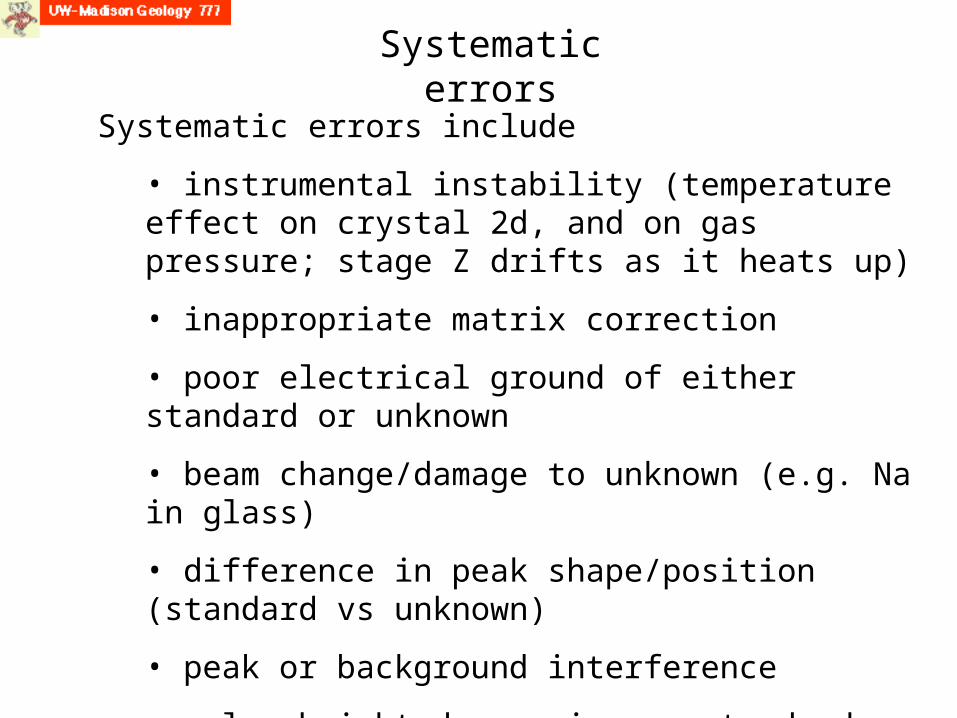
Systematic errors
Systematic errors include
• instrumental instability (temperature effect on crystal 2d, and on gas pressure; stage Z drifts as it heats up)
• inappropriate matrix correction
• poor electrical ground of either standard or unknown
• beam change/damage to unknown (e.g. Na in glass)
• difference in peak shape/position (standard vs unknown)
• peak or background interference
• pulse height depression on standard
• fluorescence across observed phase boundaries (e.g. diffusion couple)

Precision and Accuracy in Error Analysis
Precision refers to the reproducibility of the counts – and thus the ability to be able to compare compositions, whether within a sample, or between samples, or between analytical sessions. It is directly tied to counting statistics. It is a relative description.
Accuracy refers the “truth” of the analysis, and is directly tied to the standards used and the matrix correction applied to the raw data, as well most of the other variables listed previously that could affect the X-ray intensities (background and peak interferences, beam damage, etc). It is an absolute description.
EPMA quantitative error analysis is a combination of both, the first being very easy to define, the later more difficult. Precision for major elements could easily be <1%, but when combined with accuracy, total EPMA error probably 1-2% in the best cases (for major elements).
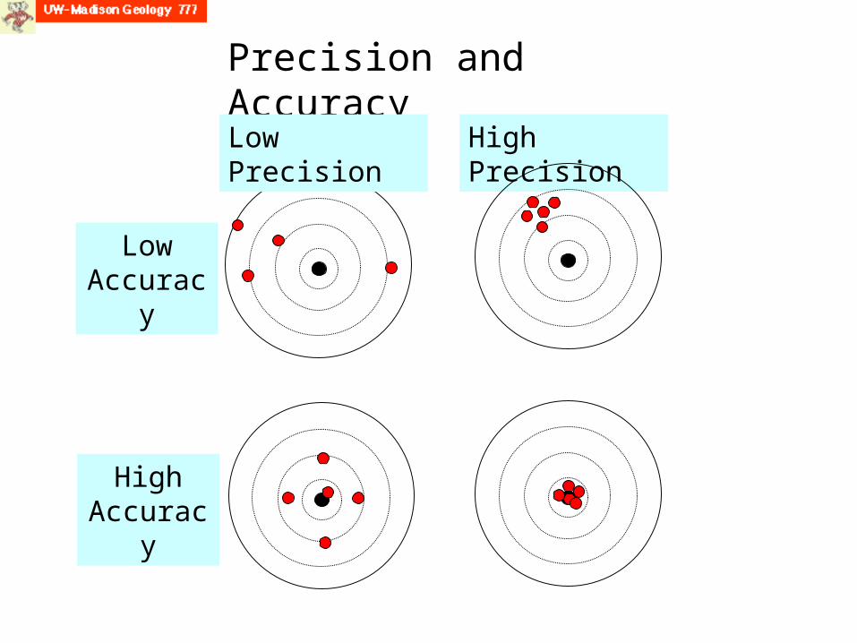
Precision and Accuracy
Low Precision High Precision
Low Accuracy
High Accuracy

Instrumental Errors-1
• Beam current stability: with Faraday cup measurements made for each analysis, long term drift should not be a problem as the counts for each analysis are normalized to a common reference current value (could be 1, or 20 nA). For long count times (minutes ) for trace element work, it is recommended that the peak and background counting be constantly cycled so that any longer period issues be spread out over the whole time period.
• Spectrometer reproducibility: with modern microprobes, this should not be a serious problem, although problems do crop up with age. Where crystals are flipped, in a small fraction of cases there is an error; generally it is not recommended to flip crystals within analyses. When spectrometer reproducibility is a problem, it is seen as backlash of the gears; to minimize errors, the peaks should always be approached from the same direction. This is set up within the software.

Instrumental Errors-2
• Thermal stability: Spectrometers could drift if there is a change in the room temperature, though this would presumably be noticeable to the operator (air conditioning fails in hot spell). I have not seen problems with PET nor LIF, though I have with TAP which could be thermal. P10 gas pressure is sensitive to the temperature change. We attempt to keep the room at 68-70°C and the circulating water temperature in the machine is very close to this. Stage height (Z) drifts due to motor heating during long (overnight) runs.
• Detector pulse height adjustment/stability: The bias (voltage) of the gold wire in the detector must be set to the proper value; this is a function of the energy of the X-ray and gas pressure. The operator must verify that the bias, gain and baseline are set properly (the last particularly where the Ar-escape peak is partially resolved).
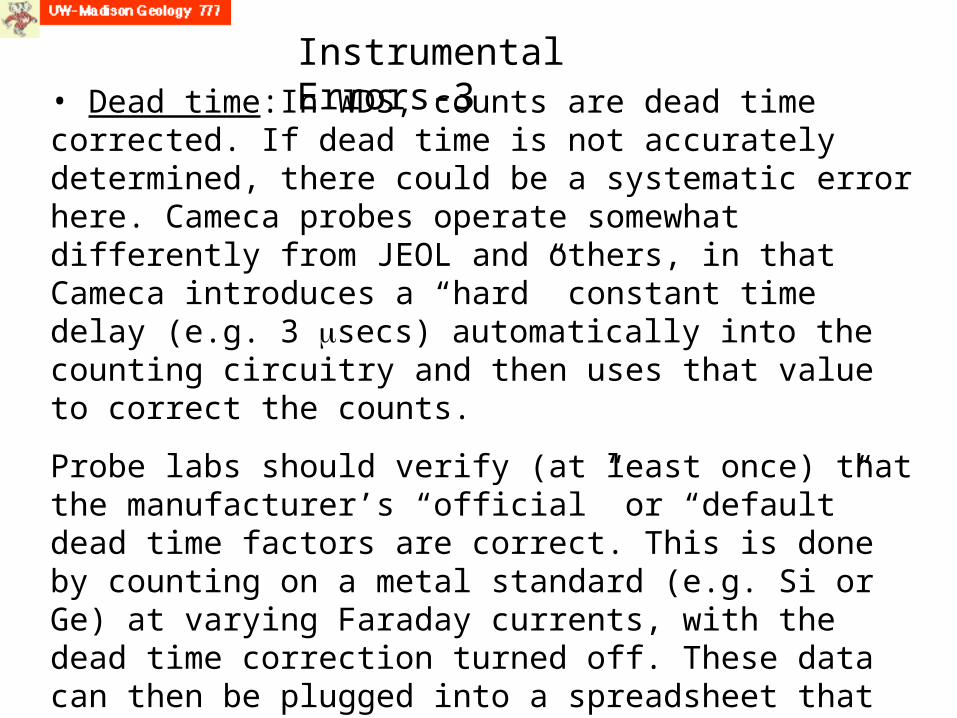
Instrumental Errors-3• Dead time:In WDS, counts are dead time corrected. If dead time is not accurately determined, there could be a systematic error here. Cameca probes operate somewhat differently from JEOL and others, in that Cameca introduces a “hard” constant time delay (e.g. 3 secs) automatically into the counting circuitry and then uses that value to correct the counts.
Probe labs should verify (at least once) that the manufacturer’s “official” or “default” dead time factors are correct. This is done by counting on a metal standard (e.g. Si or Ge) at varying Faraday currents, with the dead time correction turned off. These data can then be plugged into a spreadsheet that which Paul Carpenter (NASA) has developed to calculate the most accurate dead time actually present on a particular probe. Also, in our Probe for Windows software, there is an option for an alternate, more complex dead time correction equation, for high count rate (>50K cps)
Instrumental Errors-4
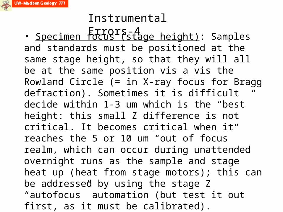
• Specimen focus (stage height): Samples and standards must be positioned at the same stage height, so that they will all be at the same position vis a vis the Rowland Circle (= in X-ray focus for Bragg defraction). Sometimes it is difficult decide within 1-3 um which is the “best” height: this small Z difference is not critical. It becomes critical when it reaches the 5 or 10 um “out of focus” realm, which can occur during unattended overnight runs as the sample and stage heat up (heat from stage motors); this can be addressed by using the stage Z “autofocus” automation (but test it out first, as it must be calibrated).
Sample/standard Error: Physical issues - 1
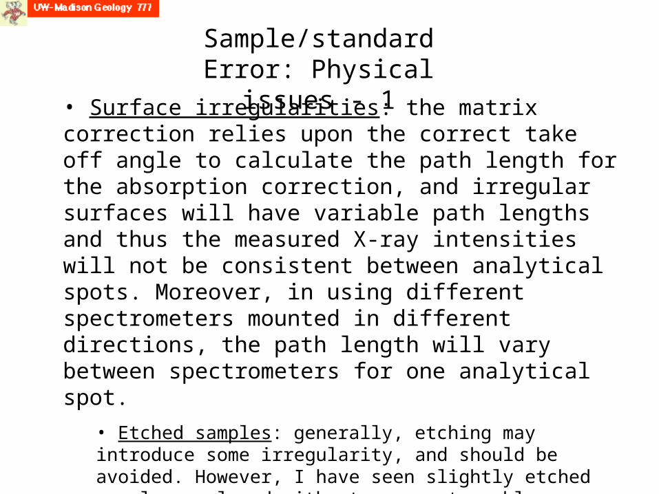
• Surface irregularities: the matrix correction relies upon the correct take off angle to calculate the path length for the absorption correction, and irregular surfaces will have variable path lengths and thus the measured X-ray intensities will not be consistent between analytical spots. Moreover, in using different spectrometers mounted in different directions, the path length will vary between spectrometers for one analytical spot.
• Etched samples: generally, etching may introduce some irregularity, and should be avoided. However, I have seen slightly etched samples analyzed without apparent problem.
• Polishing: samples should be polished with final stage using <1 m diamond or alumina or silica.
Sample/standard Error: Surface Irregularities
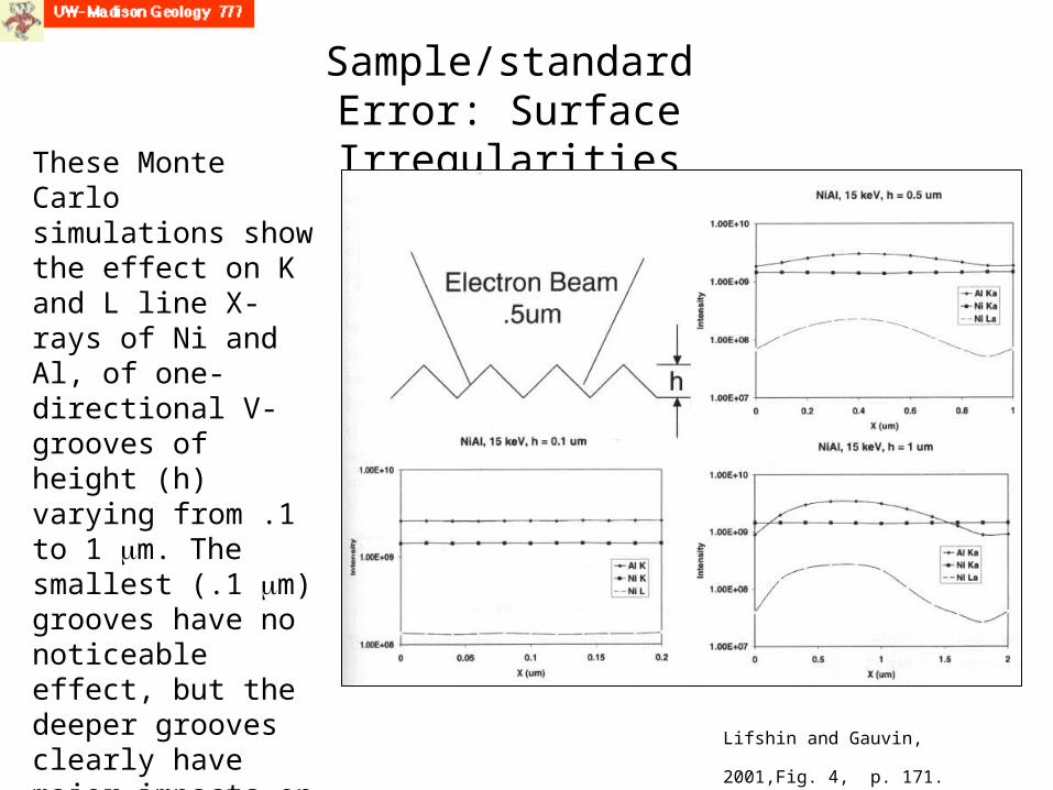
Lifshin and Gauvin, 2001,Fig. 4, p. 171.
These Monte Carlo simulations show the effect on K and L line X-rays of Ni and Al, of one-directional V-grooves of height (h) varying from .1 to 1 m. The smallest (.1 m) grooves have no noticeable effect, but the deeper grooves clearly have major impacts on Al Ka and Ni La (due to more or less absorption), with the greatest impact on the lowest energy line.

Sample/standard Error: Physical issues - 2
• Specimen homogeneity: a key assumption of quantitative EPMA is that the interaction volume is one phase (is homogeneous).
• If more than 1 phase is overlapped by the beam: the matrix correction usually overcompensates and produces an erroneous composition >100 wt%. This is common for small eutectic (groundmass) phases.
• If trace elements are being considered, then also the adjacent surrounding volume (up to ~50-100 m away) must not contain phases with higher concentrations of the elements of interest, which might be secondarily fluoresced.
• Diffusion couples have similar constraints, in that secondary fluorescence across the boundary can yield X-ray intensities up to a couple of percent (which could also give high totals). Users need to either empirically or theoretically verify this is NOT happening.

Sample/standard Error: Physical issues - 3
• Incorrect geometry (non-orthogonal surface): this occurs too often with 1” diameter plugs that have been automatically polished. For whatever reason, the sample surface ends up at a slant to the wall, and when the set screw is tightened in the holder, the surface ends up at an angle to the horizontal. This introduces an error in the take off angle. Also, the area of interest may be too low and impossible to reach stage Z focus.
Lifshin and Gauvin, 2001, Fig 3., p. 170.
This Monte Carlo simulation shows that a 5% tilt of the sample will alter the K ratio of Al Ka by .01, which equals a 8% relative error before matrix correction. An Al ZAF of 1.5 would thus increase the error to 12%.
Sample/standard Error: Physical issues - 4
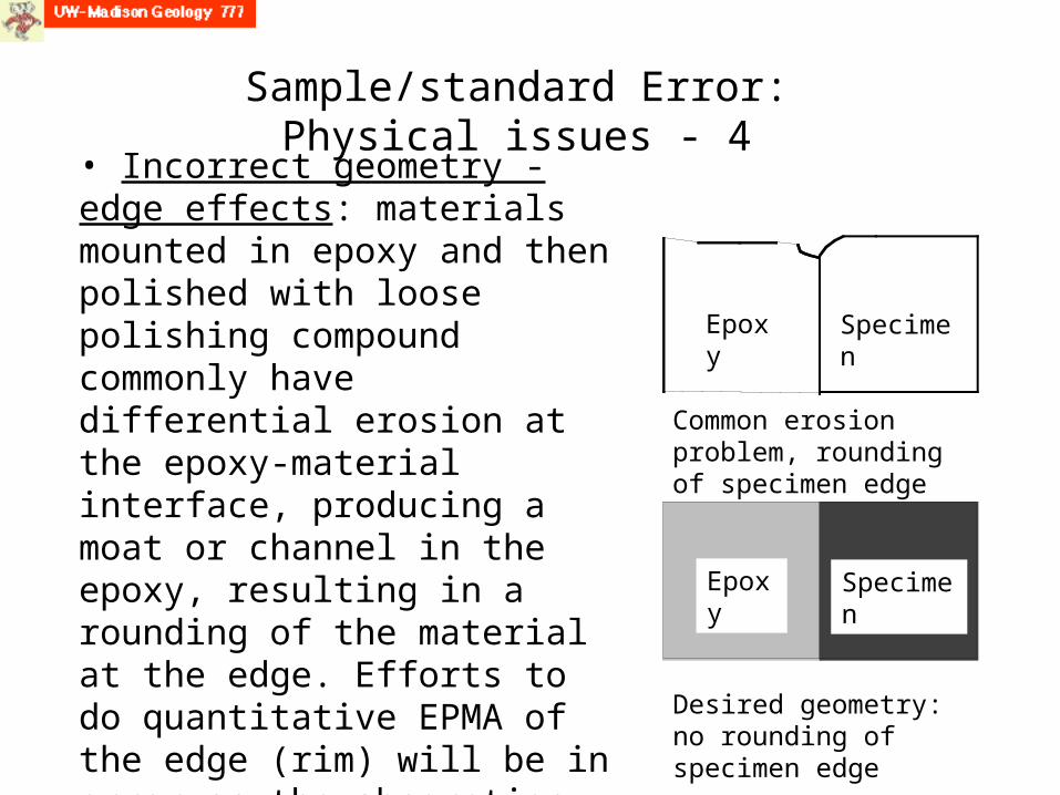
• Incorrect geometry - edge effects: materials mounted in epoxy and then polished with loose polishing compound commonly have differential erosion at the epoxy-material interface, producing a moat or channel in the epoxy, resulting in a rounding of the material at the edge. Efforts to do quantitative EPMA of the edge (rim) will be in error as the absorption path length will be non-uniform and different from the nominal length. Special polishing technique will minimize or eliminate this problem.
Epoxy
Epoxy Specimen
Specimen
Common erosion problem, rounding of specimen edge
Desired geometry: no rounding of specimen edge
Sample/standard Error: Physical issues - 5
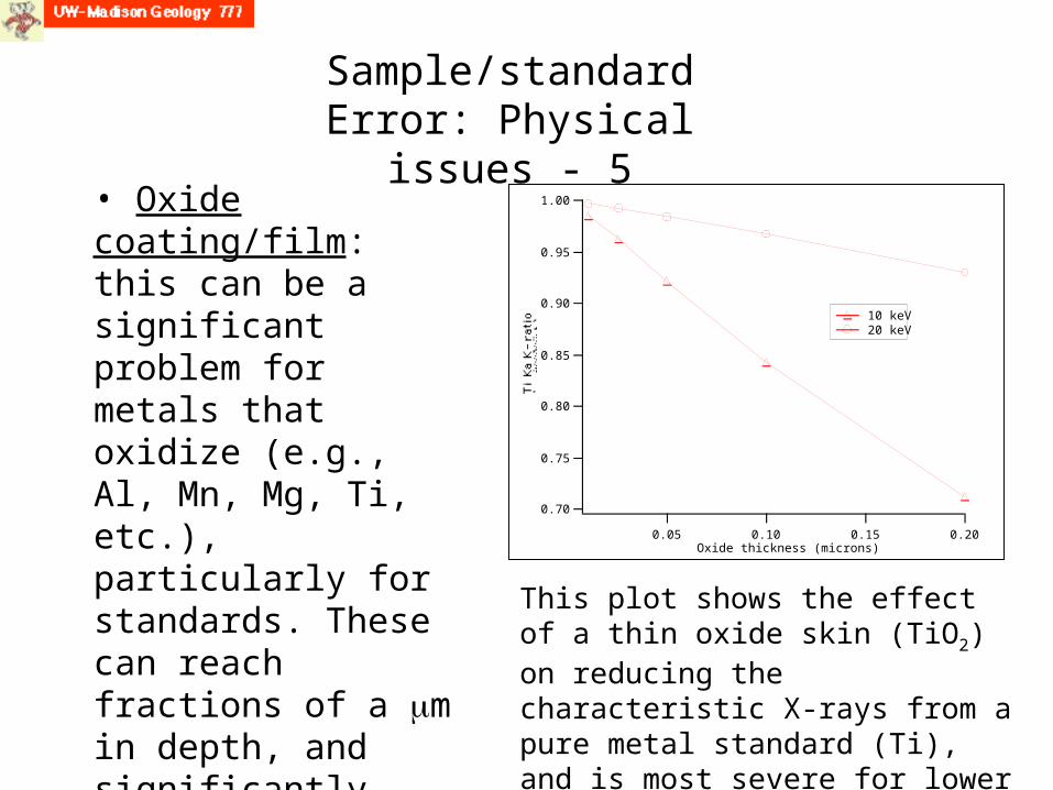
• Oxide coating/film: this can be a significant problem for metals that oxidize (e.g., Al, Mn, Mg, Ti, etc.), particularly for standards. These can reach fractions of a m in depth, and significantly alter the X-ray intensity of the line being acquired for the standard, resulting in an overestimate of the element in the unknown.
1.00
0.95
0.90
0.85
0.80
0.75
0.70
Ti Ka K-ratio
0.200.150.100.05Oxide thickness (microns)
10 keV 20 keV
This plot shows the effect of a thin oxide skin (TiO2) on reducing the characteristic X-rays from a pure metal standard (Ti), and is most severe for lower E0. (Modeled with GMRFilm software).

Sample/standard Error: Physical issues - 6
• Smear coat: soft materials may smear and cross contaminate other materials that are being polished either in the same holder, or in a subsequent sample, producing a thin ‘smear coat’. I have seen one reference in the literature to Pb or Sn smearing. It is not normally considered a major problem, at least for major element analysis.
• Polishing artifacts: Diamond and alumina polishing particles can get caught in pores in the material been polished. I have seen m fragments of brass from a brass sample holder become lodged in feldspar and biotite.
• Charging: this will reduce the effective E0 in a random manner. Conductive samples in epoxy must be grounded with conductive tape (preferred rather than paint). Semi-conductors conduct ok. Non-conductive samples need to be coated (C, Al, Ag, Be...).
• Porosity: There could be 2 errors in porous material: the electron range will be greater (absorption path longer) than in non-porous material of same composition); and in non-conductive material, there could be problems with charging as the electrons travel between pores (~vacuum) and material.

Sample/standard Error: Physical issues - 7
• Carbon coat: the conductive coating on the samples should be of the same thickness as on the standards being used. This can be evaluated experimentally or with the GMRFilm modeling program. Kerrick et al. (1973) measured the effect and showed it affected the light elements most strongly, and was worst at lower E0: a difference of 200 Å between sample and standard translated to a 4% difference in F Ka intensity. There is some antidotal evidence that old (many years-decade?) carbon coats may “go bad” (oxidize? delaminate?) and lose conductivity.
Kerrick et al, 1973, American Mineralogist, 58, 920-925.
Sample/standard Error: Physical issues - 8
• Beam sensitive samples: require care, such as lower current (e.g. 1-6 nA) and defocused beam (10-25 m), or a correction for count drop (“volatile element” correction in our Probe for Windows software):
• Glasses with alkalis (esp. Na), particularly hydrous glasses: Na drops precipitously, K somewhat, with Al and Si counts increasing .
• Alkali feldspars, particularly albite: Na counts drop
• Carbonates and anhydrite: easily decompose with 10 nA
• Apatite: not as fragile, but some grains will crater with moderate
currents (60 nA) after 40-60 seconds.
Sample/standard Error: Physical issues - 9
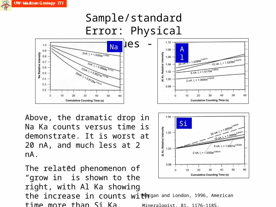
Morgan and London, 1996, American Mineralogist, 81, 1176-1185.
Above, the dramatic drop in Na Ka counts versus time is demonstrate. It is worst at 20 nA, and much less at 2 nA.
The related phenomenon of “grow in” is shown to the right, with Al Ka showing the increase in counts with time more than Si Ka.
Si
Na Al

Sample/standard Error: Physical issues - 10
• Oxidation of iron in basaltic glasses: Fialin et al (2001) reported that high electron dose (130 nA, less than 30 um diameter) led to oxidation. This was in reference to a study of Fe La/Lb as indicator of Fe-oxidation state.
• Sample orientation: Stormer et al. showed that F and Ca Ka intensities in apatite could vary with time if the electron beam was perpendicular to the c axis.
Stormer et al, 1993, American Mineralogist, 78, 641-648.

Sample/standard Error: Physical issues - 11
• Beam deflection: magnetic specimens (e.g. some Ni-Mn compounds) apparently deflect the electron beam, as seen by contamination spots offset from ‘normal’ incident position (which would affect the Rowland Circle orientation). Limited experience suggests that carbon coating as well as being rigorous in using a constant magnification (for all standards and unknowns) may help. Not much has been published on this.

Sample/standard Error: Procedural issues - 1
• Peak interferences: If measured peaks are overlapped by peaks of other elements, obvious errors will result. Such interferences can exist both in standards and unknowns. Such errors in unknowns can yield high totals. Unavoidable peak interferences must be addressed by using interference standards, to subtract the correct fraction of counts attributed to the interfering element.
• Background position interferences: Incorrect placement of background counting positions can lead to errors, as the background estimate at the peak position usually is inflated, yielding less than true counts for the element. Wavescans should be done on typical phases, and/or Virtual WDS used to evaluate the situation.

Sample/standard Error: Procedural issues - 2
• Peak shift/shape differences: We have discussed the issues of peak shifts for S Ka. Al Ka is another element with a well documented issue of differences between the metal, oxide, and alumino-silicate phases. Also F and other light elements, and L lines of Co and Ni also have such issues. Peak shifts can yield small to significant errors.
• PHA settings: Bias, gain, and baselines should be checked. Gross errors in them could produce significant errors in the analytical results. Pulse height depression occurs mainly where there is a large discrepancy in count rate between standard and unknown, e.g. 50000 cps on std B vs 500 cps on Mo-Si-B phase); count rates up to 10-15000 cps should be OK. Dropping the current on the B standard from 30 to 1 nA worked.

Counting Statistics - 1
We desire to count X-ray intensities of peak and backgrounds, for both standards and unknowns, with high precision and accuracy. X-ray production is a random process (Poisson statistics), where each repeated measurement represents a sample of the same specimen volume. The expected distribution can be described by Poisson statistics, which for large number of counts is closely approximated by the ‘normal’ (Gaussian) distribution. For Poisson distributions, 1 sigma = square root of the counts, and 68.3% of the sampled counts should fall within ±1 sigma, 95.4% within ±2 sigma, and 99.7 within ±3 sigma.
Lifshin and Gauvin, 2001, Fig. 6, p. 172
Counting Statistics-2
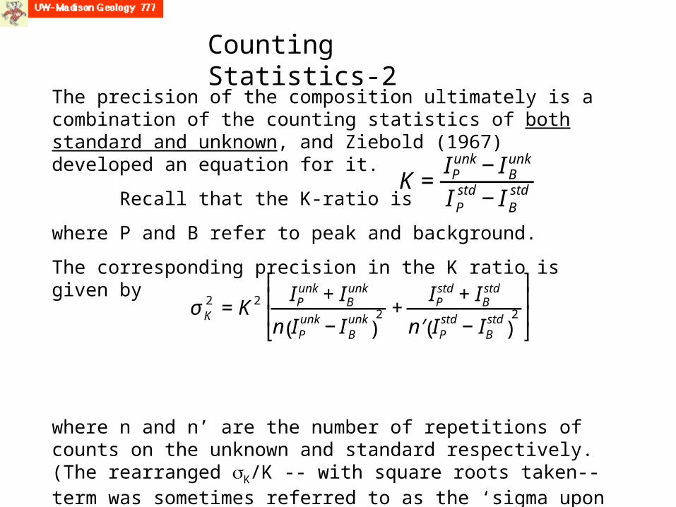
The precision of the composition ultimately is a combination of the counting statistics of both standard and unknown, and Ziebold (1967) developed an equation for it.
Recall that the K-ratio is
where P and B refer to peak and background.
The corresponding precision in the K ratio is given by
where n and n’ are the number of repetitions of counts on the unknown and standard respectively. (The rearranged K/K -- with square roots taken-- term was sometimes referred to as the ‘sigma upon K’ value.)
K =IP
unk−I Bunk
I Pstd−I B
std
σK2 =K2 IP
unk+IBunk
n IPunk−I B
unk( )
2 +IP
std+IBstd
′ n IPstd−IB
std( )
2
⎡
⎣
⎢ ⎢
⎤
⎦
⎥ ⎥

Counting Statistics-3
Another format for considering cumulative precision of the unknown is the above graph. A maximum error at the 99% confidence interval can calculated, based upon the total counts acquired upon both the standard and the unknown: e.g. to have 1% max counting error you must have at least ~120,000 counts on the unknown and on the standard; you could get 2% with ~30,000 counts on each.
From MAC shortcourse volume
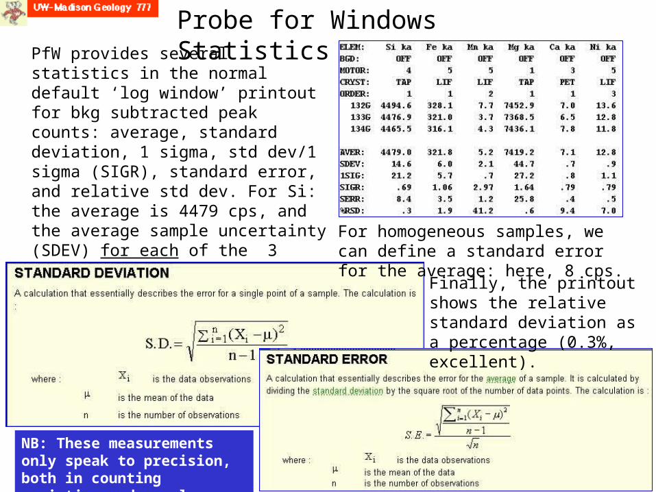
Probe for Windows Statistics -1PfW provides several statistics in the normal default ‘log window’ printout for bkg subtracted peak counts: average, standard deviation, 1 sigma, std dev/1 sigma (SIGR), standard error, and relative std dev. For Si: the average is 4479 cps, and the average sample uncertainty (SDEV) for each of the 3 measurements is 15 cps. The counting error (1 sigma) is somewhat larger (21 cps), and the ratio of std dev to sigma is <1, indicating good homogeneity in Si.
Finally, the printout shows the relative standard deviation as a percentage (0.3%, excellent).
For homogeneous samples, we can define a standard error for the average: here, 8 cps.
NB: These measurements only speak to precision, both in counting variation and sample variation.
Probe for Windows Statistics - 2
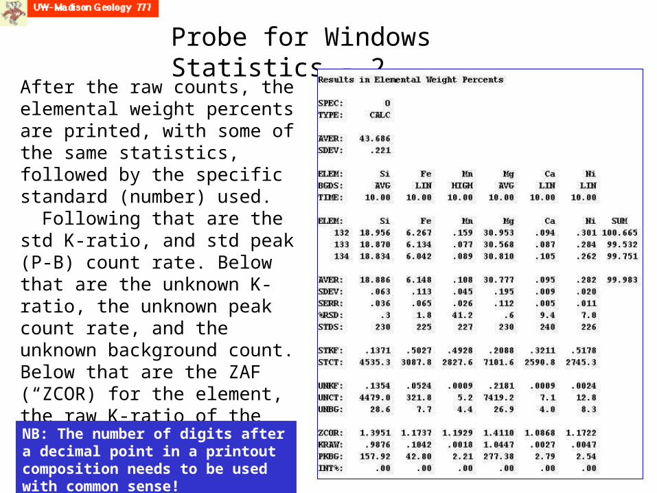
After the raw counts, the elemental weight percents are printed, with some of the same statistics, followed by the specific standard (number) used. Following that are the std K-ratio, and std peak (P-B) count rate. Below that are the unknown K-ratio, the unknown peak count rate, and the unknown background count. Below that are the ZAF (“ZCOR) for the element, the raw K-ratio of the unknown, the peak-background ratio of the unknown, and any interference correction applied (“INT%”, as percentage of measured counts).
NB: The number of digits after a decimal point in a printout composition needs to be used with common sense!

Probe for Windows Statistics - 3
PfW software provides for additional optional statistics. One set relates to detection limits, i.e. what is the lowest level you can be confident in reporting.We will deal with them later, when we talk about trace elements in a few weeks.
The other set of statistics relates to the homogeneity of the unknowns as well as calculation of analytical error. We will now discuss these statistics.
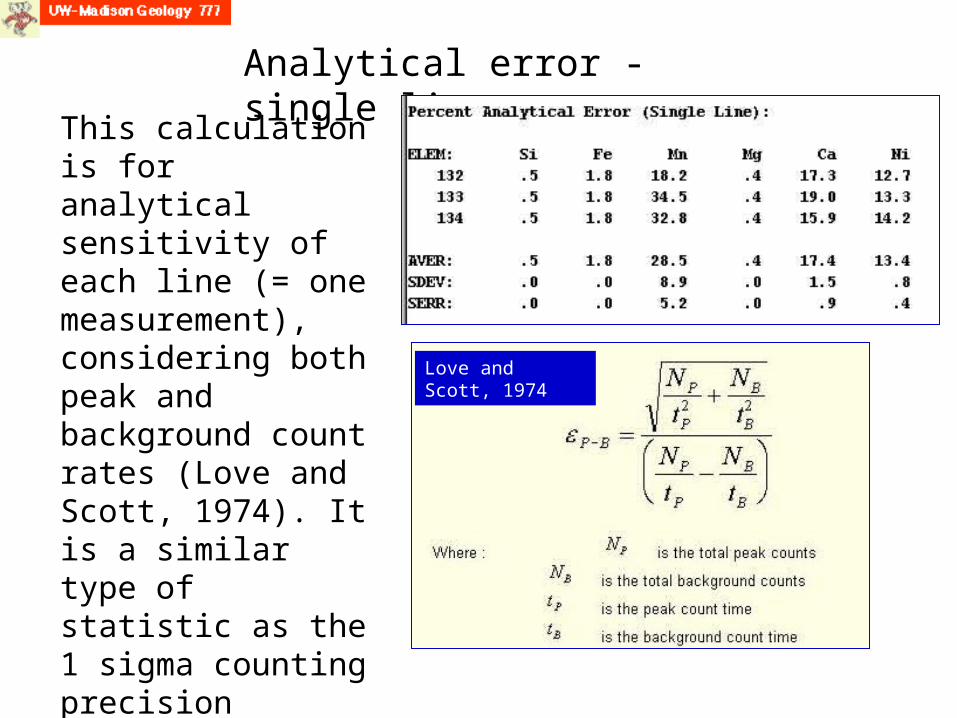
Analytical error - single line
This calculation is for analytical sensitivity of each line (= one measurement), considering both peak and background count rates (Love and Scott, 1974). It is a similar type of statistic as the 1 sigma counting precision figure, but it is presented as a percentage.
Love and Scott, 1974

Additional analytical statistics
Probe for Windows provides a more advanced set of calculations for analytical statistics. The calculations are based on the number of data points acquired in the sample and the measured standard deviation for each element. This is important because although x-ray counts theoretically have a standard deviation equal to square root of the mean, the actual standard deviation is usually larger due to variability of instrument drift, x-ray focusing errors, and x-ray production.
A common question is whether a phase being analyzed by EPMA is homogeneous, or is the same or distinct from another separate sample. An simple calculation is to look at the average composition and see if all analyses are within some range of sigmas (2 for 95%, 3 for 99% normal probability).
Homogeneity: confidence intervals
A more exacting criterion is calculating a precise range (in wt%) and level (in %) of homogeneity. These calculations utilize the standard deviation of measured values and the degree of statistical confidence in the determination of the average.
The degree of confidence means that we wish to avoid a risk of rejecting a good result a large per cent of the time (95 or 99%) of the time. “Student’s t distribution” gives various confidence levels for evaluation of data, i.e. whether a particular value could be said to be within the expected range of a population -- or more likely, whether two compositions could be confidently said to be the same. The degree of confidence is given as 1- , usually .95 or .99. This means we can define a range of homogeneity, in wt%, where on the average only 5% or 1% of repeated random points would be outside this range.

Student’s t distribution
Goldstein et al, p. 497
The general problem, where the sample size is small and the population variance is unknown, was first treated in 1905 by W.S. Gossett, who published his analysis under the pseudonym “Student”. His employer, the Guinness Breweries of Ireland, had a policy of keeping all their research as proprietary secrets. The importance of his work argued for its being published, but it was felt that anonymity would protect the company. (S.L. Meyer, Data Analysis for Scientists and Engineers, 1975, p. 274.)
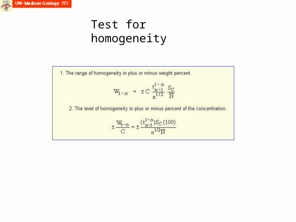
Test for homogeneity
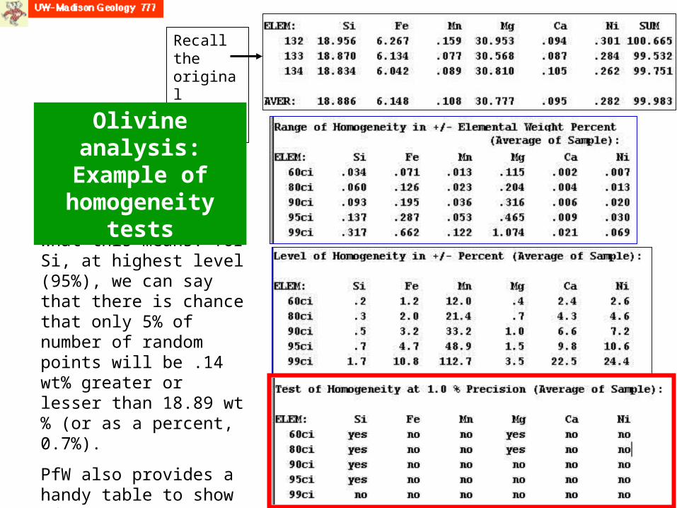
What this means: for Si, at highest level (95%), we can say that there is chance that only 5% of number of random points will be .14 wt% greater or lesser than 18.89 wt% (or as a percent, 0.7%).
PfW also provides a handy table to show if the sample is homogeneous at the 1% precision level, and if so, at what confidence level.
Recall the original analysis
Olivine analysis: Example of
homogeneity tests

Counting Statistics
Analytical sensitivity is the ability to distinguish, for an element, between two measurements that are nearly equal.
So here, at the 95% confidence level, two samples would have to have a difference in Si of > .20 wt% to be considered reliably different in Si.

Numbers of significant figures-1
There have been cases where people have taken reported compositions (i.e. wt % elements or oxides) from probe printouts and then faithfully reproduced them exactly as they got them. Once someone took figures that were reported to 3 decimal points and argued that a difference in the 3rd decimal place had some geochemical significance.
The number of significant figures reported in a printout is a “mere” programming format issue, and has nothing to do with scientific precision! (However, a recent added feature to PfW is an option to output only the actual significant number of digits. This is not normally enabled.)
Having said that, it is “tradition” to report to 2 decimal places. However, that should not be taken to represent precision, without a statistical test, such as given before.

Numbers of significant figures - 2
In the example of the olivine analysis above, where Si was printed out as 18.886 wt%, it would be reported as 18.89 -- but looking at the limited number of analyses and the homogeneity tests, I would feel uncomfortable telling someone that another analysis somewhere between 18.6 and 19.2 were not the same material. Nor would I be uncomfortable with someone reporting the Si as 18.9 wt% (though I stick to tradition.)
Considering silicate mineral or glass compositions, Si is traditionally reported with 4 significant figures. If we were to be rigorous regarding significant figures, we would follow the rule that we would be bound by the least number of figures in a calculation where we multiply our measurement (K-ratio, which will have thousands of counts divided by thousands of counts) by the ZAF. As you can appreciate there are many calculations that comprise each part of the ZAF, and it would be stretching it to argue that the ZAF itself can have more than 3 significant figures. Ergo, we should not strictly report Si with more than 3 significant figures.

Numbers of significant figures - 3
When we enable the PfW Analytical Option “Display only statistically significant number of numerical digits” for the olivine analysis, heres the result:
Wrong
For comparison, here’s the original printout:

Errors in Matrix Correction
The K-ratio is multiplied by a matrix correction factor. There are various models – alpha, ZAF, z) – and versions. Assuming that you are using the appropriate correction type, there may be some issues regarding specific parameters, e.g. mass absorption coefficients, or the z) profile.
There is a possibility of error for certain situations, particularly for “light elements” as well as compounds that have drastically different Z elements where pure element standards are used. The figure above shows that a small (2%) error in the mass absorption
Lifshin and Gauvin, 2001, p. 176.
coefficient for Al in NiAl will yield an error of 1.5% in the matrix correction.
This is a strong incentive to either use standards similar to the unknown, and/or use secondary standards to verify the correctness of the EPMA analysis.
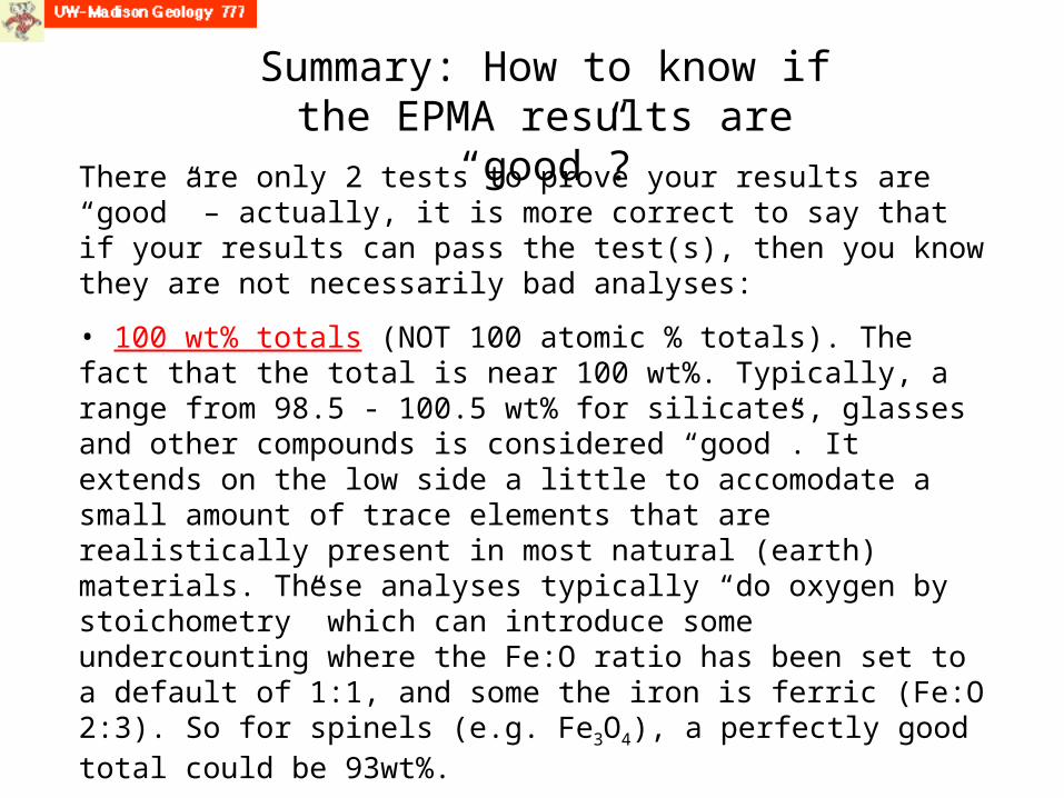
Summary: How to know if the EPMA results are “good”?
There are only 2 tests to prove your results are “good” – actually, it is more correct to say that if your results can pass the test(s), then you know they are not necessarily bad analyses:
• 100 wt% totals (NOT 100 atomic % totals). The fact that the total is near 100 wt%. Typically, a range from 98.5 - 100.5 wt% for silicates, glasses and other compounds is considered “good”. It extends on the low side a little to accomodate a small amount of trace elements that are realistically present in most natural (earth) materials. These analyses typically “do oxygen by stoichometry” which can introduce some undercounting where the Fe:O ratio has been set to a default of 1:1, and some the iron is ferric (Fe:O 2:3). So for spinels (e.g. Fe3O4), a perfectly good total could be 93wt%.
• Stoichometry, if such a test is valid (e.g. the material is a line compound, or a mineral of a set stoichometry.

• The total is excellent, 99.98 wt%
• The stoichometry is pretty good (not excellent): on the 4 oxygens, there should be 1.00 Si atoms and we have .985. The total cations Mg+Fe+Ca+Ni should be 2.00, and we have 2.03.
The analysis is OK and could be published. If this were seen at the time of analysis, it might be useful to recheck the Si and Mg peak positions , and reacquire standard counts for Si and Mg. If this were only seen after the fact, you could re-examine the
standard counts and see if there are any obvious outliers that were included and could be legitimately discarded.
Checking our olivine analysis


