Elements of Foundations for Ubiquitous Computing

Elements of Foundations for Ubiquitous Computing

the beautiful, the useful and the rest

Vladimiro Sassone

University of Southampton

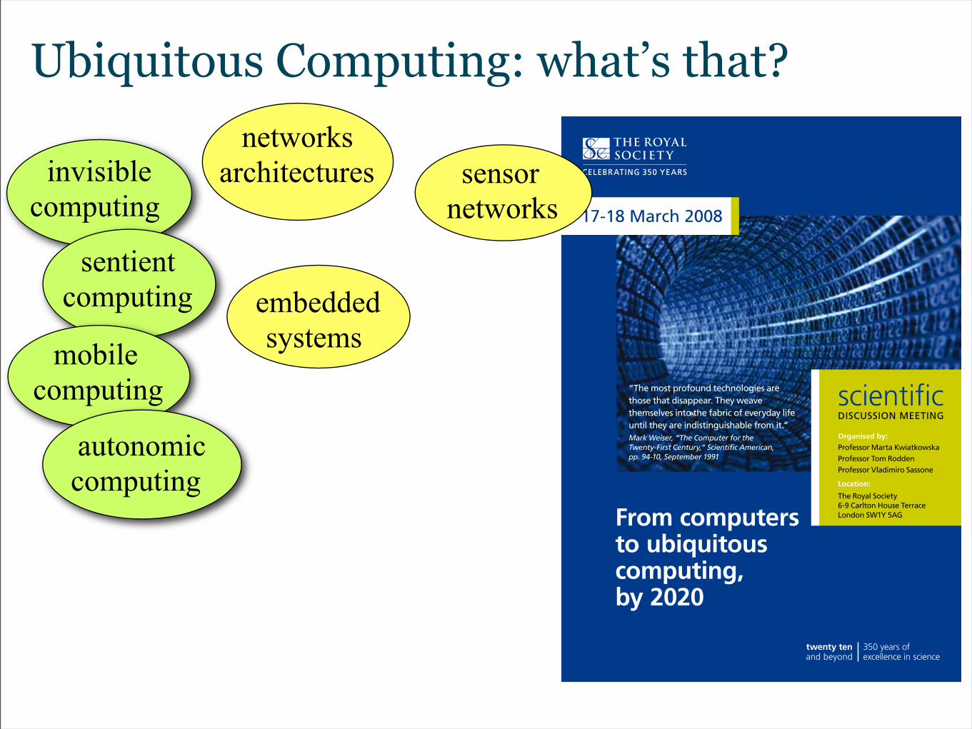
Ubiquitous Computing: what’s that?

From computers to ubiquitous computing, by 2020

scientificDISCUSSION MEETING

Organised by: Professor Marta Kwiatkowska Professor Tom RoddenProfessor Vladimiro Sassone

Location:

The Royal Society 6-9 Carlton House Terrace London SW1Y 5AG

17-18 March 2008

“The most profound technologies are those that disappear. They weave themselves into the fabric of everyday life until they are indistinguishable from it.”Mark Weiser, “The Computer for the Twenty-First Century,” Scientific American, pp. 94-10, September 1991





Location:


17-18 March 2008


invisiblecomputing





Location:


17-18 March 2008


invisiblecomputing

sentientcomputing





Location:


17-18 March 2008


invisiblecomputing

sentientcomputing

mobilecomputing





Location:


17-18 March 2008


invisiblecomputing

sentientcomputing

mobilecomputing

autonomiccomputing





Location:


17-18 March 2008


invisiblecomputing

sentientcomputing

mobilecomputing

autonomiccomputing


networks architectures sensor

networks

embeddedsystems




Location:


17-18 March 2008


invisiblecomputing

sentientcomputing

mobilecomputing

autonomiccomputing



networks

embeddedsystems

progr.languages




Location:


17-18 March 2008


invisiblecomputing

sentientcomputing

mobilecomputing

autonomiccomputing


power awareness

medicalcomputing


networks

embeddedsystems

progr.languages




Location:


17-18 March 2008


invisiblecomputing

sentientcomputing

mobilecomputing

autonomiccomputing

legal, social, ethical

issues


power awareness

medicalcomputing


networks

embeddedsystems

progr.languages




Location:


17-18 March 2008


invisiblecomputing

sentientcomputing

mobilecomputing

autonomiccomputing

legal, social, ethical

issues


privacy

crypto & securitytrust

power awareness

medicalcomputing


networks

embeddedsystems

progr.languages

A lot of embedded devices and smart space

A lot of embedded devices and smart space

Ubiquitous Computing: my perspective

Models for Concurrency

Semantic Theories

Spatial Logics

Programming Languages

Resource Control



Semantic Theories

Spatial Logics


Resource Control




Semantic Theories

Spatial Logics


Resource Control

Semantic Theories



Semantic Theories

Spatial Logics


Resource Control

Semantic TheoriesTwo related continuations:

(1) What “barbs” i.e. observations are required to give rise to an observation theory corresponding to the contexts as labels ?

(2) How to generate transition systems out of from SOS specification systems in the case of stochastic transition systems?



Semantic Theories

Spatial Logics


Resource Control

Spatial Logics



Semantic Theories

Spatial Logics


Resource Control




Semantic Theories

Spatial Logics


Resource ControlResource Control



Semantic Theories

Spatial Logics


Resource ControlResource Control

Features of Ubiquitous Computing like scalability, mobility, and incomplete information deeply affect security requirements.

One of the proposed approaches is to use a notion of computational trust, resembling the concept of trust among human beings.

Trust in UbiCom

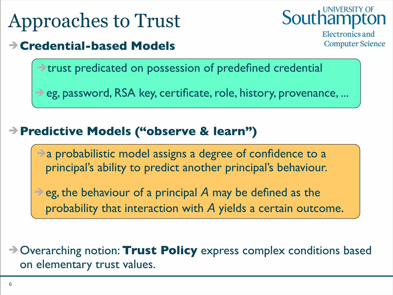
Approaches to TrustCredential-based Models

Predictive Models (“observe & learn”)

Overarching notion: Trust Policy express complex conditions based on elementary trust values.

6

trust predicated on possession of predefined credential

eg, password, RSA key, certificate, role, history, provenance, ...

a probabilistic model assigns a degree of confidence to a principal’s ability to predict another principal’s behaviour.

eg, the behaviour of a principal A may be defined as the probability that interaction with A yields a certain outcome.

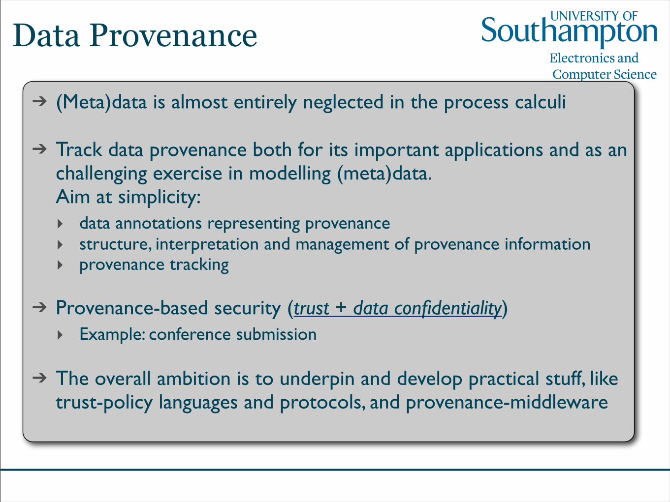
Data Provenance

➔ (Meta)data is almost entirely neglected in the process calculi

➔ Track data provenance both for its important applications and as an challenging exercise in modelling (meta)data. Aim at simplicity:‣ data annotations representing provenance‣ structure, interpretation and management of provenance information‣ provenance tracking

➔ Provenance-based security (trust + data confidentiality)‣ Example: conference submission

➔ The overall ambition is to underpin and develop practical stuff, like trust-policy languages and protocols, and provenance-middleware

Provenance model

€

v :κ

Provenance model

Annotated value

€

v :κ

Provenance model

Actual data

Annotated value

€

v :κValue

Provenance model

Actual data Meta information describing the origin of the value

Annotated value

Provenance

€

v :κValue

€

v :ε ;a!κ1 ;b?κ2 ;b!(ε;c!κ3,b?κ4 ) ;...

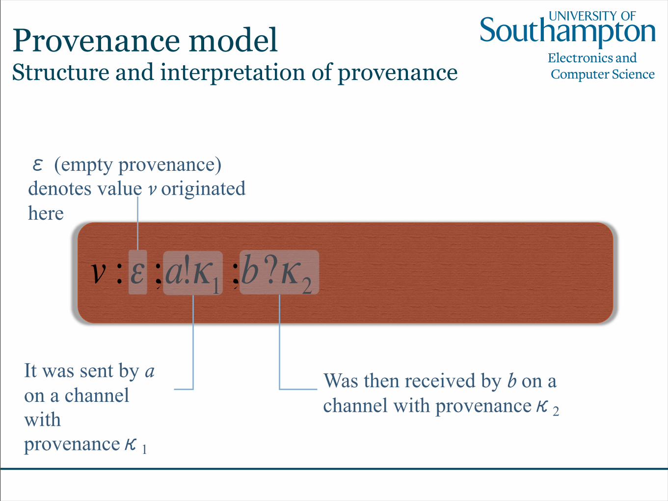
Provenance modelStructure and interpretation of provenance

€

v :ε ;a!κ1 ;b?κ2 ;b!(ε;c!κ3,b?κ4 ) ;...


ProvenanceValue

€

v :ε ;a!κ1 ;b?κ2 ;b!(ε;c!κ3,b?κ4 ) ;...


ProvenanceValue

“Operations” that were performed on the value. They record the principals that “influenced” the value and how.

€

v :ε ;a!κ1 ;b?κ2 ;b!(ε;c!κ3,b?κ4 ) ;...

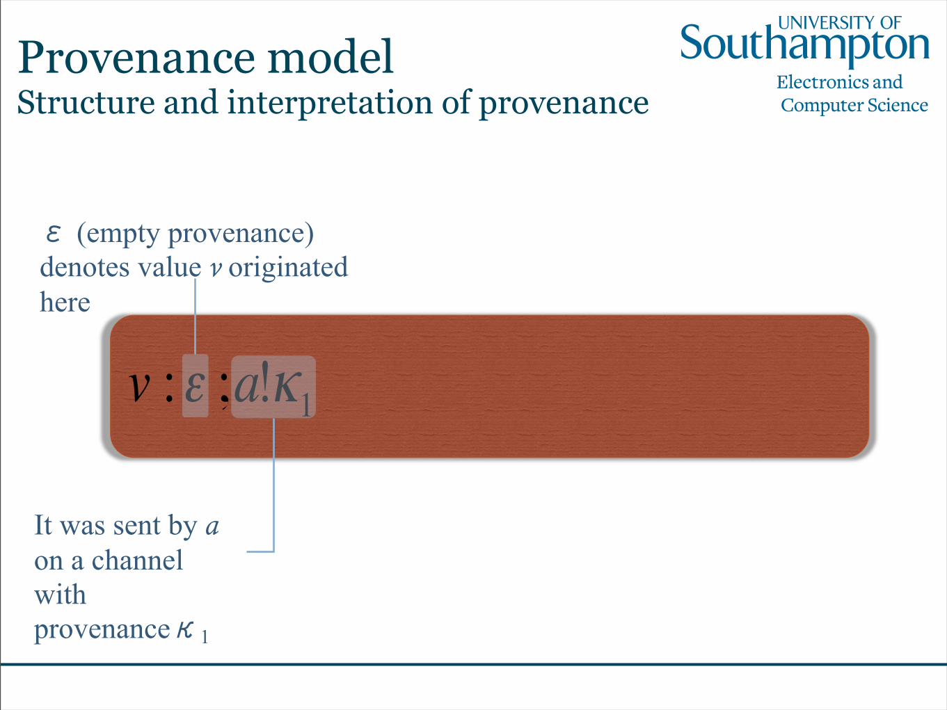
ε (empty provenance) denotes value v originated here


€

v :ε ;a!κ1 ;b?κ2 ;b!(ε;c!κ3,b?κ4 ) ;...

It was sent by a on a channel with provenanceκ1



€

v :ε ;a!κ1 ;b?κ2 ;b!(ε;c!κ3,b?κ4 ) ;...


Was then received by b on a channel with provenanceκ2



€

v :ε ;a!κ1 ;b?κ2 ;b!(ε;c!κ3,b?κ4 ) ;...


Was then received by b on a channel with provenanceκ2

And then sent by b on a channel that b received from c…



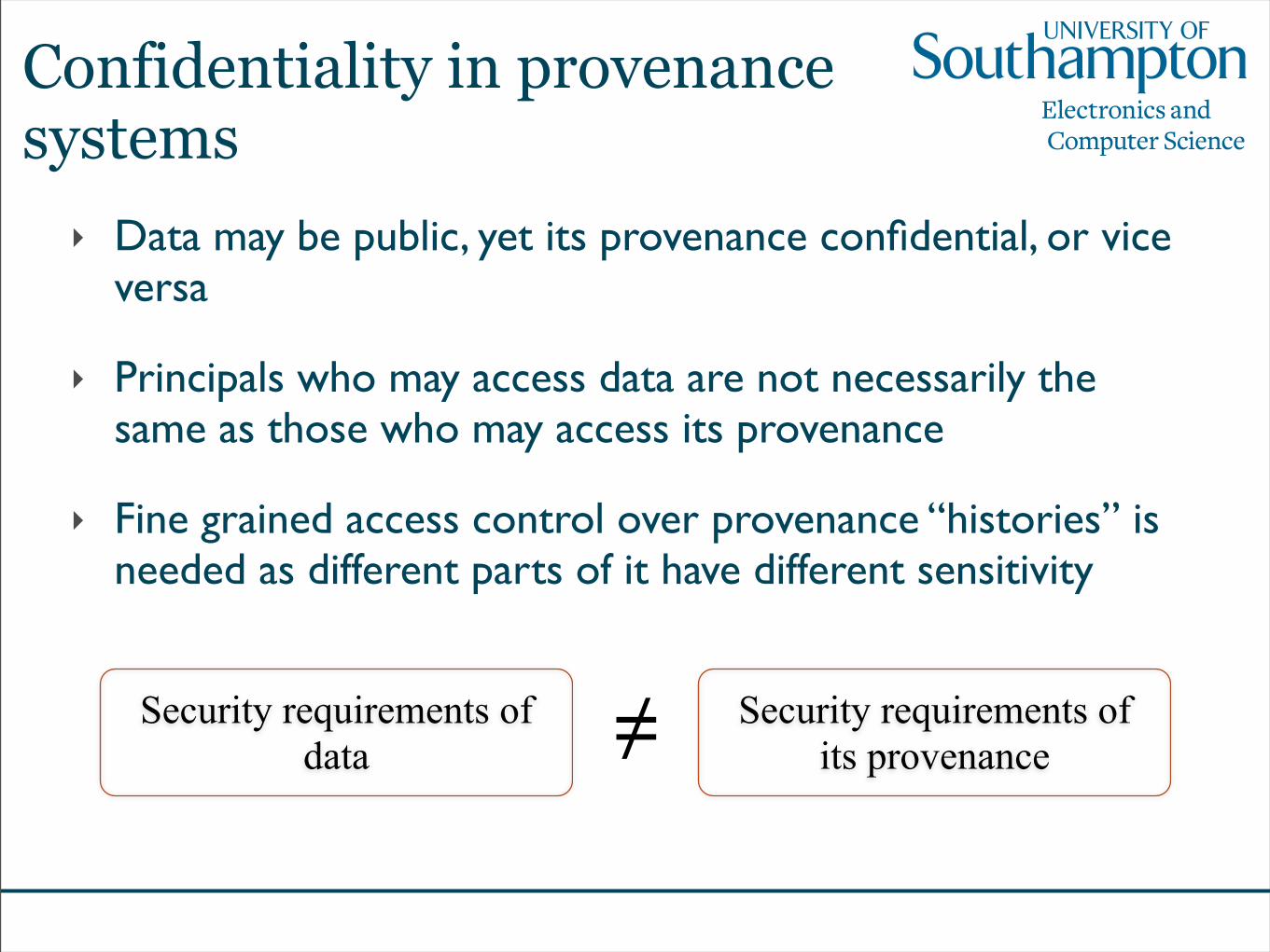
Confidentiality in provenance systems

‣ Data may be public, yet its provenance confidential, or vice versa

‣ Principals who may access data are not necessarily the same as those who may access its provenance

‣ Fine grained access control over provenance “histories” is needed as different parts of it have different sensitivity

Security requirements of data

Security requirements of its provenance≠

Hiding provenance treesExample: conference submissions

c

a

j

c: Authora: PC Chairj: Referee


c

a

j

€

entry :ε;c!κ s



c

a

j

€

entry :ε;c!κ s

€

entry :ε;c!κ s;a? ʹ′ κ s;a! ʹ′ κ r



c

a

j

€

entry :ε;c!κ s

€


€

entry :ε;c!κ s;a? ʹ′ κ s;a! ʹ′ κ r; j ? ʹ′ ʹ′ κ r; j! ʹ′ ʹ′ κ n

€

score :ε; j! ʹ′ ʹ′ κ n



c

a

j

€

entry :ε;c!κ s

€


€


€


€

entry :ε;c!κ s;a? ʹ′ κ s;a! ʹ′ κ r; j ? ʹ′ ʹ′ κ r; j! ʹ′ ʹ′ κ n;a? ʹ′ κ n;a! ʹ′ κ m

€

score :ε; j! ʹ′ ʹ′ κ n;a? ʹ′ κ n;a! ʹ′ κ m


c

a

j

€

entry :ε;c!κ s

€


€


€


€


€



c

a

j

€

entry :ε;c!κ s

€


€


€


€


€


Hidden from j


c

a

j

€

entry :ε;c!κ s

€


€


€


€


€


Hidden from jHidden from c


€


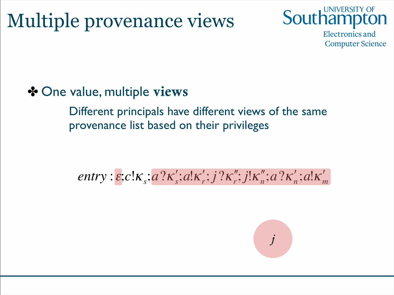
✤ One value, multiple viewsDifferent principals have different views of the same provenance list based on their privileges

Multiple provenance views

€



a


€



c


€



j


€



jca


Inferring probability distributions

22

Examples of applications in trust & security

Estimate trust in an individual or set of individuals

Estimate input distribution of a noisy channel to compute the Bayes risk

Apply the Bayesian approach to hypothesis testing (anonymity, information flow)

...

The outcome of an interaction between a principal a and a partner b is either successful or unsuccessful:

The probability that a partner b interacts successfully with a is governed by the parameter θ where:

Goal: infer (an approximation of) the probability of success Means: Observe sequence of trials (observations)

Beta Trust Model

o ∈ {Succ, Fail}

θ = Pr(o = Succ)

Beta Trust Model

Note that: the behaviour of the partner b represented by θ is assumed to be fixed over time.

The estimated probability of success, B(Succ |o), at time t is the expected value of θ given the sequence of outcomes

o = {o0, o1, . . . , ot}

B(Succ | o) = E[ θ | o ]

The “Frequentist” method:

25

Assume an a priori probability distribution for θ (representing your partial knowledge about θ, whatever the source may be) and combine it with the evidence, using Bayes’ theorem, to obtain the a posteriori distribution

F (n, s) =s

n

Using evidence to infer θ

The “Bayesian” method:

A Bayesian approach

Assumption: θ is the generic value of a continuous random variable Θ whose probability density is a Beta distribution with (unknown) parameters σ, φ

The uniform distribution is a particular case of Beta, forσ= 1, φ= 1

B(σ, φ) can be seen as the a posteriori probability density of Θ given by a uniform a priori (principle of maximum entropy) and a trial sequence resulting inσ-1 successes andφ-1 failures.

26

B(σ,ϕ)(θ) = Γ(σ+ϕ)Γ(σ)Γ(ϕ) θσ−1(1− θ)ϕ−1

where Γ is the extension of the factorial functioni.e. Γ(n) = (n− 1)! for n natural number

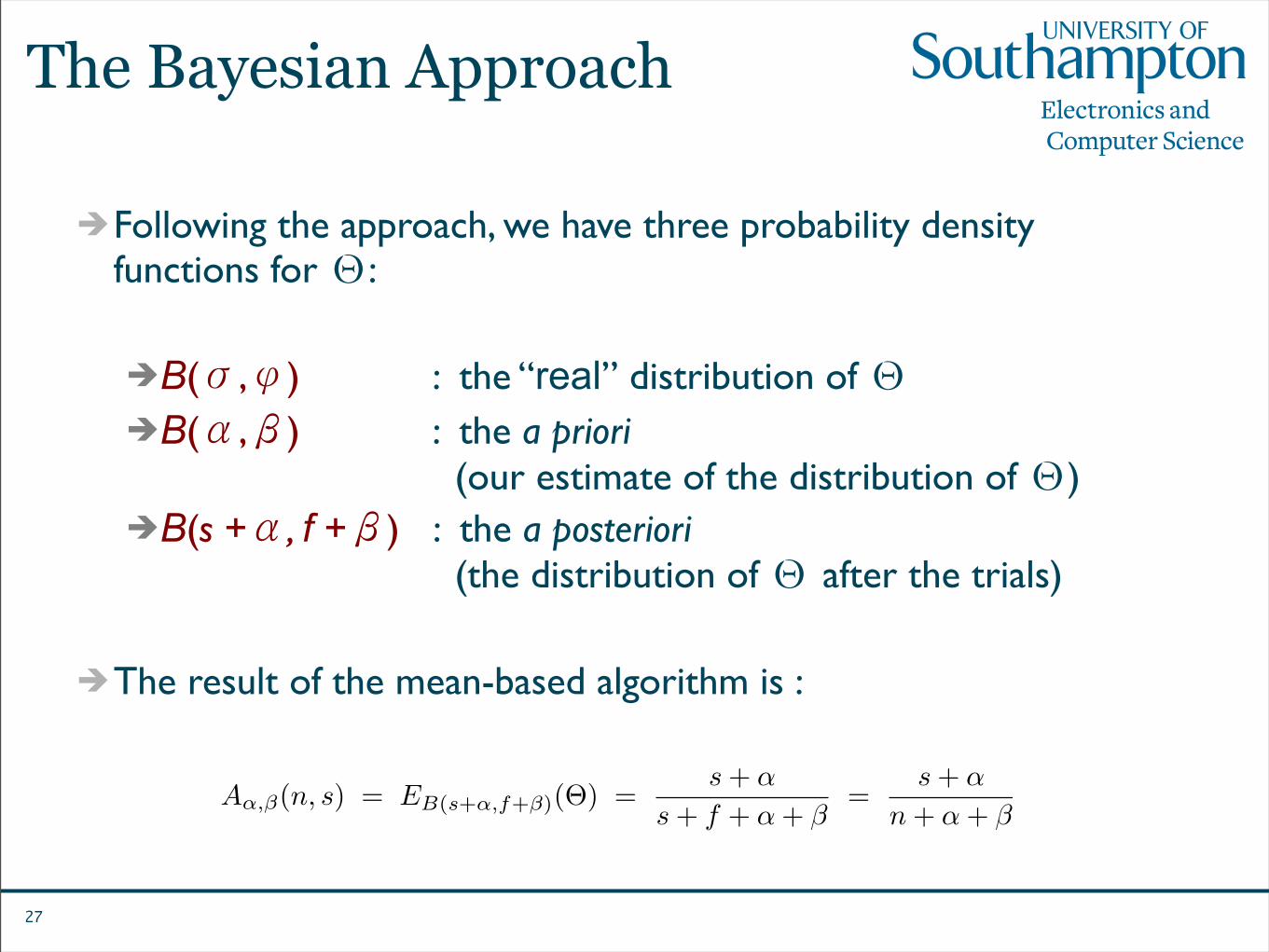
The Bayesian Approach

Following the approach, we have three probability density functions for Θ:

B(σ,φ) : the “real” distribution of ΘB(α,β) : the a priori

(our estimate of the distribution of Θ)B(s +α, f +β) : the a posteriori

(the distribution of Θ after the trials)

The result of the mean-based algorithm is :

27

Aα,β(n, s) = EB(s+α,f+β)(Θ) =s + α

s + f + α + β=

s + α

n + α + β

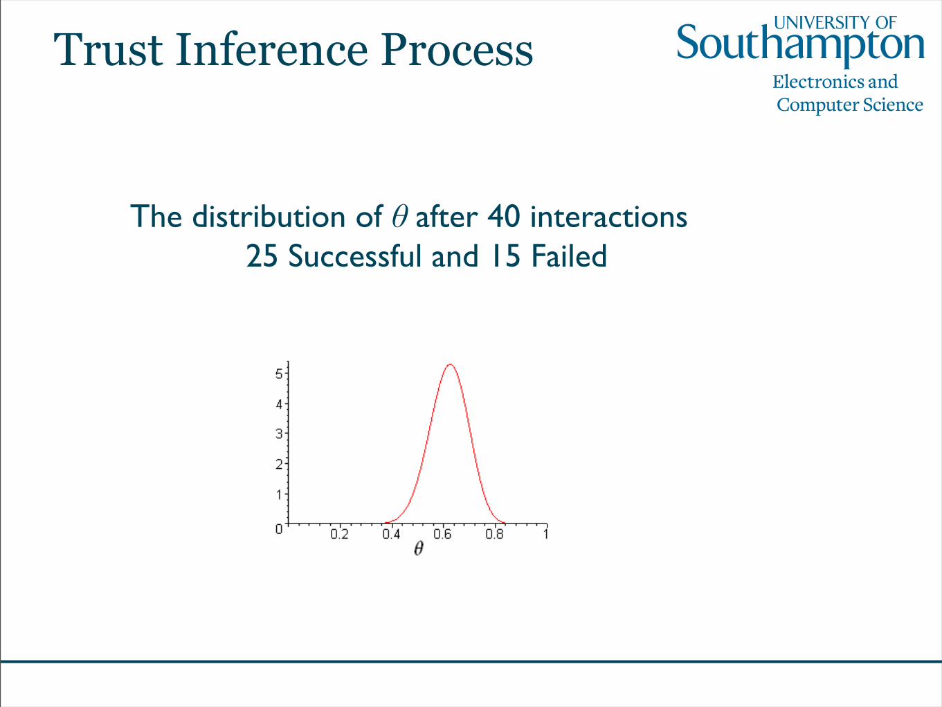
Trust Inference Process

O1= S

O2= S O3= F

O4= F O5= S

Trust Inference Process

The distribution of θ after 40 interactions 25 Successful and 15 Failed

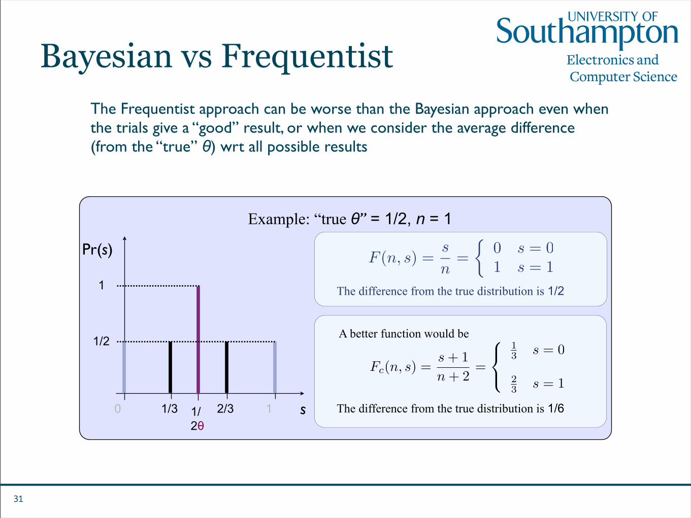
The Frequentist approach can be worse than the Bayesian approach even when the trials give a “good” result, or when we consider the average difference (from the “true” θ) wrt all possible results

30

Example: “true θ” = 1/2, n = 1

1/2θ

s10

1/2

1

Pr(s)

The difference from the true distribution is 1/2

F (n, s) =s

n=

�0 s = 01 s = 1

Bayesian vs Frequentist

31


1/2θ

s10

1/2

1

Pr(s)


F (n, s) =s

n=

�0 s = 01 s = 1

1/3 2/3

A better function would be


Fc(n, s) =s + 1n + 2

=

13 s = 0

23 s = 1



32


1/2θ

s10

1/4

1

Pr(s)

1/2

The average difference from the true distribution is 1/4

F (n, s) =s

n=

0 s = 012 s = 11 s = 2



33


1/2θ

s10

1/4

1

Pr(s)

1/2

The average distance from the true distribution is 1/4

F (n, s) =s

n=

0 s = 012 s = 11 s = 2

1/4 3/4

Again, a better function would be

The average distance from the true distribution is 1/8

Fc(n, s) =s + 1n + 2

=

14 s = 0

12 s = 1

34 s = 2



Define a “difference’’ D(A(n,s),θ) (not necessarily a distance) non-negative zero iff A(n,s) =θ

Consider the expected value DE(A,n,θ) of D(A(n,s),θ) with respect to the likelihood (the conditional probability of s |θ)

Risk of A : the expected value R(A,n) of DE(A,n,θ) with respect to the “true” distribution of Θ

34

DE(A,n, θ) =n�

s=0

Pr(s | θ) D(A(n, s), θ)

R(A,n) =� 1

0Pd(θ) DE(A,n, θ) dθ

Measuring the precision of Bayesian algorithms

We have considered the following candidates for D(x,y) (all of which can be extended to the n-ary case):

The norms: |x - y| |x - y|2

... |x - y|k

... The Kullback-Leibler divergence

35

DKL((y, 1− y) � (x, 1− x)) = y log2y

x+ (1− y) log2

1− y

1− x


Theorem. For the mean-based Bayesian algorithms, with a priori B(α,β), we have that the condition is satisfied (i.e. the Risk is minimum when α,β coincide with the parameters σ, φ of the “true” distribution), by the following functions:

The 2nd norm (x - y)2

The Kullback-Leibler divergence

Surprising that the condition is satisfied by these two very different functions, and not by any of the other norms |x - y|k for k≠2.

It leaves the search open for a measure for assessment and comparison of trust algorithm.

36


Potential applications

We can use DE to compare two different estimation algorithms; develop a measure of quality for “decision-making” algorithms

Mean-based vs other ways of selecting a θ

Bayesian vs non-Bayesian

In more complicated scenarios there may be different Bayesian mean-based algorithms; eg.: noisy channels.

37

Potential applications (ctd)

DE induces a metric on distributions. Bayes’ equations define transformations on this metric space from the a priori to the a posteriori.

Study the properties of such transformations to reveal interesting properties of the corresponding Bayesian methods, independent of the a priori.

Hypothesis testing (privacy, anonymity, confidentiality, information flow analysis, input distribution analysis, ...) :

determine (probabilistic) bounds as to what probability-distribution inference algorithm may determine about you, your online activity, your software

38

Limitation of the Beta model

The assumption that a principal behaviour is fixed is not always realistic:

The behaviour of a principal may depend on its internal state which may change over time.

Modelling Dynamic Behaviour

Modelling static behaviour as a probability distribution over outcomes leads to modelling the dynamic behaviour by a Hidden Markov Model (HMM).

A single state in an HMM models the system behaviour at a particular time.

Hidden Markov Model:

A simpler model: Beta with Decay

The probability distribution over outcomes changes over time.

Old observations are given less weight (decayed) than more

recent observations.

Weights of observations are controlled by the decay factor r.

Beta Trust Model with Decay

Given a decay factor 0 ≤ r <1 and an observation sequence o={o0,…,oL} then

Br(Succ | o) =mr(o) + 1

mr(o) + nr(o) + 2Br(Fail | o) =

mr(o) + 1mr(o) + nr(o) + 2

where

mr(o) =L�

i=0

rL−i · δSucc(oi) nr(o) =L�

i=0

rL−i · δFail(oi)

andδx(o) =

�1 if x = o0 otherwise

How good is the model ?

Given a dynamic system modelled by an HMM λ we define Beta estimation error as follows

where r is the decay factor, and α is the real probability that next outcome is Success

Error(λ, r) = E�(B(Succ | o)− α)2

�

System stability

System stability is the expected probability of the HMM remaining in the same state.

Consider the system modelled by HMM:

Unstable system

Stable system

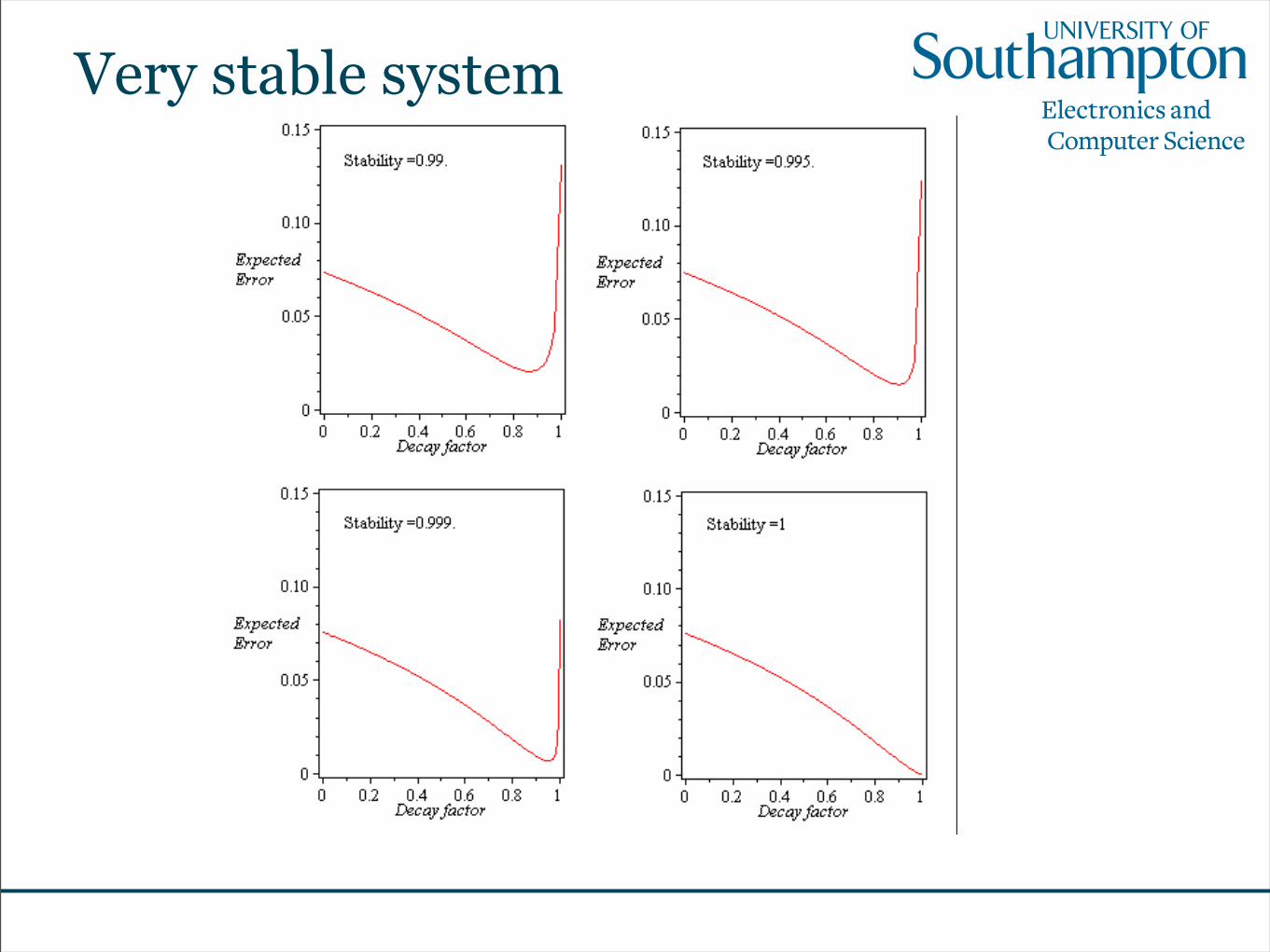
Very stable system

Conclusion (in general)

49

A whole wholly-different conception of computing to be developed: hard to talk of “further” work in general

Chiefly, nowhere like here apps w/out sound models are dangerous, and theory without practice is pointless


49



The gap between Theory and Practice matters in practice(although it may not matter in theory)


49



The gap between Theory and Practice matters in practice(although it may not matter in theory)

One thing I know: as one cannot “model-check” UbiNet, security & privacy in UbiCom must be coupled with trust

Conclusion (personal take)

50

in the short term:‣ hiding and multiview in provenance trees ‣ measures suitable to compare trust-algorithms‣ reputation in HMMs‣ integration of anonymity protocols and trust

in the longer term:‣ programming language bindings‣ data confidentiality and then privacy‣ ...‣ ...

Date post:	16-Oct-2021
Category:	Documents
Upload:	others
View:	2 times
Download:	0 times

Elements of Foundations for Ubiquitous Computing

Documents