EMPIRICAL ANALYSIS OF INNOVATION IN OLIGOPOLY INDUSTRIES Lectures 4 and 5: Dynamic strategic behavior in rmsinnovation CEMFI SUMMER SCHOOL 2018 Victor Aguirregabiria (University of Toronto) September 6-7, 2018 Victor Aguirregabiria () Consumer value new products September 6-7, 2018 1 / 132
Transcript
EMPIRICAL ANALYSIS OF INNOVATIONIN OLIGOPOLY INDUSTRIES
Lectures 4 and 5:Dynamic strategic behavior in firms’innovation
CEMFI SUMMER SCHOOL —2018Victor Aguirregabiria (University of Toronto)
September 6-7, 2018
Victor Aguirregabiria () Consumer value new products September 6-7, 2018 1 / 132
Lectures 4-5: Dynamic strategic behavior in firms’innovation
Dynamic strategic behavior in firms’innovation: Outline
1. Competition and Innovation: static analysis
2. Dynamic games of oligopoly competition
3. Creative destruction and the incentives to innovate ofincumbents and new entrants
4. Competition and innovation in the CPU industry: Intel andAMD
5. Environmental regulation and adoption of green technologies
Victor Aguirregabiria () Consumer value new products September 6-7, 2018 2 / 132
Victor Aguirregabiria () Consumer value new products September 6-7, 2018 3 / 132
Competition and Innovation: static analysis
Competition and Innovation
Long lasting debate on the effect of competition on innovation (e.g.,Schumpeter, Arrow).
Apparently, there are contradictory results between a good number oftheory papers showing that "competition" has a negative effect oninnovation (Dasgupta & Stiglitz, 1980: Spence, 1984), and a goodnumber of reduced-form empirical papers showing a positiverelationship between measures of competition and measures ofinnovation (Porter, 1990; Geroski, 1990; Blundell, Griffi th and VanReenen 1999).
Vives (JIND, 2008) presents a systematic theoretical analysis of thisproblem that tries to explain the apparent disparaty between existingtheoretical and empirical results.
Victor Aguirregabiria () Consumer value new products September 6-7, 2018 4 / 132
Competition and Innovation: static analysis
Competition and Innovation: Vives (2008) [2]
Vives considers:
[1] Different sources of exogenous increase in competition.(i) reduction in entry cost; (ii) increase in market size; (iii)
increase in degree of product substitutability.
[2] Different types of innovation.(i) process or cost-reduction innovation; (ii) product innovation /
new products.
[3] Different models of competition and specifications.(i) Bertrand; (ii) Cournot
[4] Specification of demandlinear, CES, expontetial, logit, nested logit.
Victor Aguirregabiria () Consumer value new products September 6-7, 2018 5 / 132
Competition and Innovation: static analysis
Competition and Innovation: Vives (2008) [3]
Vives shows that- [1] the form of increase in competition- and [2] the type of innovation
are key to detemine a positive or a negative relatioship betwweencompetition and innovation.
However, the results are very robust:[3] the form of competition (Bertrand or Cournot)and [4] the specification of the demand system.
Victor Aguirregabiria () Consumer value new products September 6-7, 2018 6 / 132
Competition and Innovation: static analysis
Vives (2008): Model
Static model with symmetric firms, endogenous entry.
c(zj ) = marginal cost (constant); zi = expenditure in cost reduction;c ′ < 0 and c ′′ > 0
F = entry cost
Victor Aguirregabiria () Consumer value new products September 6-7, 2018 7 / 132
Competition and Innovation: static analysis
Equilibrium
Nash equilibrium for simultaneous choice of (pj , zj ). Symmetricequilibrium. There is endogenous entry.
Marginal condition w.r.t cos-reduction R&D (z) is: −c ′(z) sd(p, n; α)− 1 = 0. Since c ′′ > 0, this implies
z = g(s d(p, n; α))
where g(.) is an increasing function.
The incentive to invest in cost reduction increases with output perfirm, q ≡ s d(p, n; α).
Victor Aguirregabiria () Consumer value new products September 6-7, 2018 8 / 132
Competition and Innovation: static analysis
Equilibrium (2)
Any exogenous change in competition (say in α, s, or F ) has threeeffects on output per firm and therefore on investment incost-reduction R&D.
dzdα
= g ′(q)[
∂ [s d(p, n; α)]∂α
+∂ [s d(p, n; α)]
∂p∂p∂α+
∂ [s d(p, n; α)]∂n
∂n∂α
]∂ [s d(p, n; α)]
∂αis the direct demand effect,
∂ [s d(p, n; α)]∂p
∂p∂αis the price pressure effect.
∂ [s d(p, n; α)]∂n
∂n∂αis the number of entrants effect.
The effects of different changes in competition on cost-reductionR&D can be explained in terms of these three effects.
Victor Aguirregabiria () Consumer value new products September 6-7, 2018 9 / 132
Competition and Innovation: static analysis
Summary of comparative statics
(i) Increase in market size.- Increases per-firm expenditures in cost-reduction;- Effect on product innovation (# varieties) can be either positive ornegative.
(ii) Reduction in cost of market entry.- Reduces per-firm expenditures in cost-reduction;- Increases number of firms and varieties.
(iii) Increase in degree of product substitution.- Increases per-firm expenditures in cost-reduction;- # varieties may increase or decline.
Victor Aguirregabiria () Consumer value new products September 6-7, 2018 10 / 132
Competition and Innovation: static analysis
Some limitations in this analysis
The previous analysis is static, without uncertainty, with symmetricand single product firms.
Therefore, the following factors that relate competition andinnovation are absent from the analysis.
(1) Preemptive motives.
(2) Cannibalization of own products.
(3) Increasing uncertainty in returns to R&D due competition(asymmetric info).
To study these factors, we need dynamic games with uncertainty, andasymmetric multi-product firms.
Victor Aguirregabiria () Consumer value new products September 6-7, 2018 11 / 132
Victor Aguirregabiria () Consumer value new products September 6-7, 2018 12 / 132
Dynamic games of oligopoly competition
Dynamic games of oligopoly competition
Firms compete in investment decisions that have returns in thefuture, involve substantial uncertainty, and can have important effectson competitors‘profits.
Understanding the dynamic strategic interactions between firmsdecisions (e.g., dynamic complementarity or substitutability) isimportant to understand the forces behind the dynamics of anindustry or to evaluate policies.
Empirical dynamic games provide a framework to study thesequestions and perform policy analysis.
Victor Aguirregabiria () Consumer value new products September 6-7, 2018 13 / 132
Dynamic games of oligopoly competition
Some recent applications of DG to innovation
Competition in R&D and product innovation between Intel and AMD:Goettler and Gordon (JPE, 2011).
Product innovation of incumbents and new entrants in the hard driveindustry: Igami (JPE, 2017).
Complementarities between investment in R&D and exporting: Aw,Roberts, and Xu (AER, 2011).
Product differentiation and innovation in the automobile industry:Hasmi & Van Biesebroeck (RStat, 2016).
Victor Aguirregabiria () Consumer value new products September 6-7, 2018 14 / 132
Dynamic games of oligopoly competition Basic Framework and Assumptions
Dynamic Games: Basic Structure
• Follows the framework in Ericson-Pakes (1995).
• Time is discrete and indexed by t. The game is played by N firms[potential entrants] that we index by i .
• Firms compete in two different dimensions: a static dimension and adynamic dimension.
• We denote the dynamic dimension as the "investment decision".
Victor Aguirregabiria () Consumer value new products September 6-7, 2018 15 / 132
Dynamic games of oligopoly competition Basic Framework and Assumptions
Dynamic Games: Basic Structure (2)
• Let ait be the variable that represents the investment decision of firm iat period t.
• This investment decision can be an entry/exit decision, R&D, productquality, etc.
• Every period, firms observed the state variables (e.g., their capitalstocks) and compete in prices or quantities in a static Cournot or Bertandmodel.
• Let pit be the static decision variables (e.g., price) of firm i at period t.
Victor Aguirregabiria () Consumer value new products September 6-7, 2018 16 / 132
Dynamic games of oligopoly competition Basic Framework and Assumptions
Dynamic Games: Basic Structure (3)
• I start presenting a simple dynamic game of market entry-exit and"quality" choice where every period incumbent firms compete a laBertrand.
• The dynamic investment decision ait ∈ {0, 1, ..., J} represents the R&Dor quality choice if ait > 0, and ait = 0 if the firm is not active in themarket at period t.
• The action is taken to maximize the expected and discounted flow ofprofits in the market,
Et (∑∞r=0 δr Πit+r )
where δ ∈ (0, 1) is the discount factor, and Πit is firm i’s profit at periodt.
Victor Aguirregabiria () Consumer value new products September 6-7, 2018 17 / 132
Dynamic games of oligopoly competition Basic Framework and Assumptions
Profit function
• The profits of firm i at time t are given by
Πit = VPit − FCit − ECit − ICit + SVit
where:VPit represents variable profit;FCit is the fixed cost of operating;ECit is a one time entry costICit is an investment costSVit is the exit value of scrap value
Victor Aguirregabiria () Consumer value new products September 6-7, 2018 18 / 132
Dynamic games of oligopoly competition Basic Framework and Assumptions
Variable profit function
• The variable profit VPit is an "indirect" variable profit function thatcomes from the equilibrium of a static Bertrand game with differentiatedproduct.
• The marginal cost is ci (ait , zt ), where zt is the a vector of exogenousstate variables, and produces a product with quality vi (ait , zt ).
• Consumer utility of buying product i is uit = νi (ait , zt )− α(zt ) pit + εit ,where νi (.) and α(.) are functions, and εit is a consumer-specific i.i.d.extreme value type 1 random variable.
Victor Aguirregabiria () Consumer value new products September 6-7, 2018 19 / 132
Dynamic games of oligopoly competition Basic Framework and Assumptions
Variable profit function (2)
• The variable profit of an active firm is:
VPit = (pit − ci (ait , zt )) qit
where pit and qit represent the price and the quantity sold by firm i atperiod t, respectively.
Victor Aguirregabiria () Consumer value new products September 6-7, 2018 21 / 132
Dynamic games of oligopoly competition Basic Framework and Assumptions
Model: Variable profit function (4)
• Equilibrium prices depend on the vector of product qualities of the activefirms in the market (at), and on the exogenous variables zt :p∗it = p
∗i (at , zt ).
• Similarly, the equilibrium market shares s∗it is a function of (at , zt ):s∗it = s
∗i (at , zt ).
• Therefore, the indirect or equilibrium variable profit of an active firm is:
VPit = ait Ht (p∗i (at , zt )− ci (zt )) s∗i (at , zt )
= ait Ht θVPi (at , zt )
where θVPi (.) is a function that represents variable profits per capita.
Victor Aguirregabiria () Consumer value new products September 6-7, 2018 22 / 132
Dynamic games of oligopoly competition Basic Framework and Assumptions
Fixed cost
• The fixed cost is paid every period that the firm is active in the market,and it has the following structure (mode of entry-exit):
FCit = 1{ait > 0}[θFCi (ait , zt ) + εFCit (ait )
]• θFCi (ait , zt ) is a function that represents the fixed operating cost of firmi if it produces a product with quality ait . zt is a vector of exogenous statevariables that are common knowledge to all the firms.
• εFCit (ait ) are a zero-mean shocks that is private information of firm i .
Victor Aguirregabiria () Consumer value new products September 6-7, 2018 23 / 132
Dynamic games of oligopoly competition Basic Framework and Assumptions
Fixed cost (2)
• There are two main reasons why we incorporate these privateinformation shocks in the model.
• First, as shown in Doraszelski and Satterthwaite (2012), it is a way toguarantee that the dynamic game has at least one equilibrium in purestrategies.
• Second, they are convenient econometric errors. If private informationshocks are independent over time and over players, and unobserved to theresearcher, they can ’explain’players heterogeneous behavior withoutgenerating endogeneity problems.
Victor Aguirregabiria () Consumer value new products September 6-7, 2018 24 / 132
Dynamic games of oligopoly competition Basic Framework and Assumptions
Entry cost
• The entry cost is paid only if the firm was not active in the market atprevious period (entry-exit model):
]• θECi (ait , zt ) is a function that represents the entry cost of firm i ifthe initial product quality is ait .
• εECit (ait ) are private information shocks in the entry cost
Victor Aguirregabiria () Consumer value new products September 6-7, 2018 25 / 132
Dynamic games of oligopoly competition Basic Framework and Assumptions
Investment cost
• There are also costs of adjusting the level of quality, or repositioningproduct characteristics. For instance,
ICit = 1{ait−1 > 0}(
θAC (+)i (zt ) 1{ait > ait−1}+ θ
AC (−)i (zt ) {ait < ait−1}
)• θ
AC (+)i (zt ) and θ
AC (−)i (zt ) represents the costs of increasing and
reducing quality, respectively, once the firm is active.
• In this specification the adjustment costs are lump-sum. We couldconsider more flexible specifications with (asymmetric) linear, quadratic,and lump-sum ACs.
Victor Aguirregabiria () Consumer value new products September 6-7, 2018 26 / 132
Dynamic games of oligopoly competition Basic Framework and Assumptions
State variables
• The payoff relevant state variables of this model are:
• (1) the exogenous state variables affecting demand and costs, zt ,and market size Ht . For notational simplicity, we represent them in thevector zt
• (2) the previous qualities of all the firmsat−1 ≡ {ait−1 : i = 1, 2, ...,N};
• (3) the private information shocks {εit : i = 1, 2, ...,N}.
Victor Aguirregabiria () Consumer value new products September 6-7, 2018 27 / 132
Dynamic games of oligopoly competition Basic Framework and Assumptions
State variables (2)
• The specification of the model is completed with the transition rules ofthese state variables.
• (1) Exogenous state variables follow an exogenous Markov processwith transition probability function Fz (zt+1|zt ).
• (2) The transition of the qualitiy choices is trivial in this model. Wecould extend it to stochastic evolution. However, note that future returnsof investment in quality is uncertain.
• (3) Private information shock εit is i.i.d. over time and independentacross firms with CDF Gi .
Victor Aguirregabiria () Consumer value new products September 6-7, 2018 28 / 132
Dynamic games of oligopoly competition Basic Framework and Assumptions
Timing of decisions and state variables
• In this example, firms’dynamic decisions are made at the beginning ofperiod t and they are effective during the same period.
• An alternative timing that has been considered in many applications isthat there is a one-period time-to-build, i.e., the decision is made at periodt, and entry costs are paid at period t, but the firm is not active in themarket until period t + 1. This is in fact the timing of decisions in Ericsonand Pakes (1995).
• All the results below can be easily generalized to this model withtime-to-build.
Victor Aguirregabiria () Consumer value new products September 6-7, 2018 29 / 132
Dynamic games of oligopoly competition Markov Perfect Equilibrium
Markov Perfect Equilibrium
• Most of the recent literature in IO studying industry dynamics focuseson studying a Markov Perfect Equilibrium (MPE), as defined by Maskinand Tirole (Econometrica, 1988).
• The key assumption in this solution concept is that players’strategiesare functions of only payoff-relevant state variables.
• In this model, the payoff-relevant state variables for firm i are(yt , zt , εit ).
• We use xt to represent the vector of common knowledge state variables,i.e., xt ≡ (yt , zt ).
Victor Aguirregabiria () Consumer value new products September 6-7, 2018 30 / 132
Dynamic games of oligopoly competition Markov Perfect Equilibrium
Markov Perfect Equilibrium (2)
• Let α = {αi (xt , εit ) : i ∈ {1, 2, ...,N}} be a set of strategy functions,one for each firm.
• A MPE is a set of strategy functions α∗ such that every firm ismaximizing its value given the strategies of the other players.
• For given strategies of the other firms, the decision problem of a firm isa single-agent dynamic programming (DP) problem.
Victor Aguirregabiria () Consumer value new products September 6-7, 2018 31 / 132
Dynamic games of oligopoly competition Markov Perfect Equilibrium
Markov Perfect Equilibrium (3)
• Let V αi (xt , εit ) be the value function of the DP problem that describes
the best response of firm i to the strategies α−i of the other firms.
• This value function is the unique solution to the Bellman equation:
V αi (xt , εit ) = maxait
Παi (ait , xt )− εit (ait )
+δ∫V αi (xt+1, εit+1) dGi (εit+1) F
αi (xt+1|ait , xt )
where Πα
i (ait , xt ) and Fαi (xt+1|ait , xt ) are the expected one-period profit
and the expected transition of the state variables, respectively, for firm igiven the strategies of the other firms.
Victor Aguirregabiria () Consumer value new products September 6-7, 2018 32 / 132
Dynamic games of oligopoly competition Markov Perfect Equilibrium
Markov Perfect Equilibrium (4)
• For the quality choice game, the expected one-period profit Παi (ait , xt )
• vαi (ait , xt ) is the conditional choice value function that represents the
value of firm i if: (1) the other firms behave according to their strategiesin α; and (2) the firm chooses alternative ait today and then behavesoptimally forever in the future.
vαi (ait , xt ) ≡ Πα
i (ait , xt ) + δ∫V αi (xt+1, εit+1) dGi (εit+1) F
αi (xt+1|ait , xt )
Victor Aguirregabiria () Consumer value new products September 6-7, 2018 34 / 132
Dynamic games of oligopoly competition Markov Perfect Equilibrium
Markov Perfect Equilibrium (6)
• A Markov perfect equilibrium (MPE) in this game is a set of strategyfunctions α∗ such that for any player i and for any (xt , εit )we have that:
α∗i (xt , εit ) = argmaxait
{vα∗i (ait , xt )− εit (ait )
}
Victor Aguirregabiria () Consumer value new products September 6-7, 2018 35 / 132
Dynamic games of oligopoly competition Conditional Choice Probabilities
Conditional Choice Probabilities
• Given a strategy function αi (xt , εit ), we can define the correspondingConditional Choice Probability (CCP) function as :
Pi (a|x) ≡ Pr (αi (xt , εit ) = a | xt = x)
=∫1{αi (xt , εit ) = a} dGi (εit )
• From now on, we use CCPs to represent players’strategies, and use theterms ’strategy’and ’CCP’as interchangeable.
Victor Aguirregabiria () Consumer value new products September 6-7, 2018 36 / 132
Dynamic games of oligopoly competition Conditional Choice Probabilities
MPE in terms of CCPs
• A MPE is a vector of CCPs, P ≡ {Pi (a|x) : for any (i , a, x)}, such that:
Pi (a|x) = Pr(a = argmax
ai
{vPi (ai , x)− εi (ai )
}| x)
• vPi (ai , x) is a conditional choice probability function, but it has a slightlydifferent definition that before. Now, vPi (ai , x) represents the value of firmi if the firm chooses alternative ai today and
all the firms, including firm i , behave according to their respectiveCCPs in P.
• Every MPE in this dynamic game can be represented using this mapping.
Victor Aguirregabiria () Consumer value new products September 6-7, 2018 37 / 132
Dynamic games of oligopoly competition Conditional Choice Probabilities
MPE in terms of CCPs (2)
• The form of this equilibrium mapping depends on the distribution of εi .
• For instance, in the entry/exit model, if εi is N(0, 1):
Pi (1|x) = Φ(vPi (1, x)− vPi (0, x)
)
• In the model with endogenous quality choice, if εi (a)’s are extreme valuetype 1 distributed:
Pi (a|x) =exp
{vPi (a, x)
}∑Jj=0 exp
{vPi (j , x)
}
Victor Aguirregabiria () Consumer value new products September 6-7, 2018 38 / 132
Creative destruction: incentives to innovate of incumbents and newentrants (Igami, 2017)
Victor Aguirregabiria () Consumer value new products September 6-7, 2018 39 / 132
Creative destruction: incentives to innovate of incumbents and newentrants (Igami, 2017) Introduction
Innovation and creative destruction (Igami, 2017)
• Innovation, the creation of new products and technologies, necessarilyimplies the "destruction" of existing products, technologies, and firms.
• In other words, the survival of existing products / technologies / firms isat the cost of preemting the birth of new ones.
• The speed (and the effectiveness) of the innovation process in anindustry depends crucially on the dynamic strategic interactions between"old" and "new" products/technologies.
• Igami (JPE, 2017) studies these interactions in the context of theHard-Disk-Drive (HDD) industry during 1981-1998.
Victor Aguirregabiria () Consumer value new products September 6-7, 2018 40 / 132
Creative destruction: incentives to innovate of incumbents and newentrants (Igami, 2017) Introduction
HDD: Different generations of products
Victor Aguirregabiria () Consumer value new products September 6-7, 2018 41 / 132
Creative destruction: incentives to innovate of incumbents and newentrants (Igami, 2017) Introduction
HDD: Different generations of products
Victor Aguirregabiria () Consumer value new products September 6-7, 2018 42 / 132
Creative destruction: incentives to innovate of incumbents and newentrants (Igami, 2017) Introduction
Adoption new tech: Incumbents vs. New Entrants
Victor Aguirregabiria () Consumer value new products September 6-7, 2018 43 / 132
Creative destruction: incentives to innovate of incumbents and newentrants (Igami, 2017) Introduction
Adoption new tech: Incumbents vs. New Entrants
• Igami focuses on the transition from 5.25 to 3.5 inch products.
• He consider three main factors that contribute to the relative propensityto innovate of incumbents and potential entrants.
Cannibalization. For incumbents, the introduction of a new productreduces the demand for their pre-existing products.Preemption. Early adoption by incumbents can deter entry andcompetition from potential new entrants.Differences in entry/innovation costs. It can play either way.Incumbents have knowledge capital and economies of scope, but theyalso have organizational inertia.
Victor Aguirregabiria () Consumer value new products September 6-7, 2018 44 / 132
Creative destruction: incentives to innovate of incumbents and newentrants (Igami, 2017) Data
Market shares New/Old products
Victor Aguirregabiria () Consumer value new products September 6-7, 2018 45 / 132
Creative destruction: incentives to innovate of incumbents and newentrants (Igami, 2017) Data
Average Prices: New/Old products
Victor Aguirregabiria () Consumer value new products September 6-7, 2018 46 / 132
Creative destruction: incentives to innovate of incumbents and newentrants (Igami, 2017) Data
Average Quality: New/Old products
Victor Aguirregabiria () Consumer value new products September 6-7, 2018 47 / 132
Creative destruction: incentives to innovate of incumbents and newentrants (Igami, 2017) Data
Market Structure: New/Old products
Victor Aguirregabiria () Consumer value new products September 6-7, 2018 48 / 132
Creative destruction: incentives to innovate of incumbents and newentrants (Igami, 2017) Model
Model
• Market structure at period t is described by four type of firms accordingto the products they produce:
st = {Noldt , Nbotht , Nnewt , Npet }
• Initialy, Nboth0 = Nnew0 = 0.• Timing within a period t:1. Incumbents compete (a la Cournot) → Period profits πt (sit , s−it )2. The Noldt firms draw private info shocks and simultaneously chooseaoldit ∈ {exit, stay , innovate}3. The Nbotht observe aoldt , draw private info shocks, and simultaneouslychoose abothit ∈ {exit, stay}4. The Nnewt observe aoldt , abotht ,draw private info shocks, andsimultaneously choose anewit ∈ {exit, stay}5. The Npet observe aoldt , abotht , anewt , draw private info shocks, andsimultaneously choose apeit ∈ {entry , noentry}.
Victor Aguirregabiria () Consumer value new products September 6-7, 2018 49 / 132
Creative destruction: incentives to innovate of incumbents and newentrants (Igami, 2017) Model
Model [2]
• Given these choices, next period market structure is obtained, st+1, anddemand and cost variables evolve exogenously.
• Why imposing this order of move? This Assumption, together with:- Finite horizon T ,- Homogeneous firms (up to the i.i.d. private info shocks) withing
each type,implies that there is a unique Markov Perfect equilibrium.
• This is very convenient for estimation (Igami uses a standard/RustNested Fixed Point Algorithm for estimation) and especially forcounterfactuals.
Victor Aguirregabiria () Consumer value new products September 6-7, 2018 50 / 132
Creative destruction: incentives to innovate of incumbents and newentrants (Igami, 2017) Model
Model: Demand
• Simple logit model of demand. A product is defined as a pair{technology, quality}, where technology ∈ {old , new} and qualityrepresents different storage sizes.
• There is no differentiation across firms (perhaps true, but assumptioncomes from data limitations).
• Estimation:
ln(sjsk
)= α1 [pj − pk ] + α2
[1newj − 1newk
]+ α3 [xj − xk ] + ξ j − ξk
• Data: multiple periods and regions.• IVs: Hausman-Nevo. Prices in other regions.
Victor Aguirregabiria () Consumer value new products September 6-7, 2018 51 / 132
Creative destruction: incentives to innovate of incumbents and newentrants (Igami, 2017) Model
Estimates of Demand
Victor Aguirregabiria () Consumer value new products September 6-7, 2018 52 / 132
Creative destruction: incentives to innovate of incumbents and newentrants (Igami, 2017) Model
Evolution of unobserved Quality (epsi)
Victor Aguirregabiria () Consumer value new products September 6-7, 2018 53 / 132
Creative destruction: incentives to innovate of incumbents and newentrants (Igami, 2017) Model
Evolution of Marginal Costs
Victor Aguirregabiria () Consumer value new products September 6-7, 2018 54 / 132
Creative destruction: incentives to innovate of incumbents and newentrants (Igami, 2017) Model
Evolution of Period Profits [keeping market structure]
Victor Aguirregabiria () Consumer value new products September 6-7, 2018 55 / 132
Creative destruction: incentives to innovate of incumbents and newentrants (Igami, 2017) Model
Estimates of Dynamic Parameters
Victor Aguirregabiria () Consumer value new products September 6-7, 2018 56 / 132
Creative destruction: incentives to innovate of incumbents and newentrants (Igami, 2017) Model
Estimates of Dynamic Parameters
• Different estimates depending on the order of move within a period.
• Cost for innovation is smaller for incumbents than for new entrants(κinc < κpe ). Organizational inertia does not seem an important factor.
• Magnitude of entry costs are comparable to the annual R&D budget ofspecialized HDD manufacturers, e.g., Seagate Tech: between$0.6B − $1.6B.
Victor Aguirregabiria () Consumer value new products September 6-7, 2018 57 / 132
Creative destruction: incentives to innovate of incumbents and newentrants (Igami, 2017) Model
Estimated Model: Goodness of fit
Victor Aguirregabiria () Consumer value new products September 6-7, 2018 58 / 132
Creative destruction: incentives to innovate of incumbents and newentrants (Igami, 2017) Model
Counterfactual: Removing Cannibalization
Victor Aguirregabiria () Consumer value new products September 6-7, 2018 59 / 132
Creative destruction: incentives to innovate of incumbents and newentrants (Igami, 2017) Model
Counterfactual: Removing Preemption
Victor Aguirregabiria () Consumer value new products September 6-7, 2018 60 / 132
Competition and innovation in the CPU industry: Intel and AMD(Goettler & Gordon, 2011)
Victor Aguirregabiria () Consumer value new products September 6-7, 2018 61 / 132
Introduction
Introduction
Study competition between Intel and AMD in the PC microprocessorindustry.
Incorporates durability of the product as a potentially importantfactor.
Two forces drive innovation:- competition between firms for the technological frontier;
- since PCs have little physical depreciacion, firms have theincentive to innovate to generate a tenological depreciation ofconsumers’installed PCs that encourages them to upgrade [most ofthe demand during the period >89% was upgrading].
Duopolists face both forces, whereas a monopolist faces only thelatter (but in a stronger way).
Victor Aguirregabiria () Consumer value new products September 6-7, 2018 62 / 132
Introduction The PC microprocessor industry
The PC microprocessor industry
Very important to the economy:- Computer equipment manufacturing industry generated 25% of
U.S. productivity growth from 1960 to 2007.
Innovations in microprocessors are directly measured via improvedperformance on benchmark tasks. Most important: CPU speed.
Interesting also from the point of view of antitrust:- In 2004: several antitrust lawsuits claiming Intel’s
anticompetitive practices, e.g., rewarding PC manufacturers thatexclusively use Intel microprocessors.
- Intel foreclosures AMD to access some consumers.- Intel settled these claims in 2009 with a $1.25 billion payment
to AMD.
Victor Aguirregabiria () Consumer value new products September 6-7, 2018 63 / 132
Introduction The PC microprocessor industry
The PC microprocessor industry (2)
Market is essentially a duopoly, with AMD and Intel selling 95%CPUs.
Firmst have high R&D intensities, R&D/Revenue (1993-2004):- AMD 20% ; and Intel 11%
Innovation is rapid: new products are released nearly every quarter.
CPU performance (speed) doubles every 7 quarters, i.e., Moore’e law.
AMD and Intel extensively cross-license each other’s technologies,i.e., positive spillovers.
Victor Aguirregabiria () Consumer value new products September 6-7, 2018 64 / 132
Introduction The PC microprocessor industry
The PC microprocessor industry (3)
As microprocessors are durable, replacement drives and importantpart of demand.
The importance of replacement is partly exogenous (new consumersarriving to the marker), and partly endogenous: speed ofimprovements in frontier microprocessors that encourages consumersto upgrade.
In 2004, 82% of PC purchases were replacements.
After an upgrade boom, prices and sales fall as replacement demanddrops. Firms must continue to innovate to rebuild replacementdemand.
Victor Aguirregabiria () Consumer value new products September 6-7, 2018 65 / 132
Introduction Data
Data
Proprietary data from a market research firm specializing in themicroprocessor industry.
Quarterly data from Q1-1993 to Q4-2004 (48 quarters).
Information on: shipments in physical units for each type of CPU;manufacturers’average selling prices (ASP); production costs; CPUcharacteristics (speed).
All prices and costs are converted to base year 2000 dollars.
Quarterly R&D investment levels, obtained from firms’annual reports.
Victor Aguirregabiria () Consumer value new products September 6-7, 2018 66 / 132
Introduction Data
Moore’s Law
Intel cofounder Gordon Moore predicted in 1965 that the number oftransistors ina CPU (and therefore the CPU speed) would doubleevery 2 years.
Following figure shows “Moore’s law”over the 48 quarters in the data.
Quality is measured using processor speed.
Quarterly % change in CPU speed is 10.2% for Intel and 11% forAMD.
Victor Aguirregabiria () Consumer value new products September 6-7, 2018 67 / 132
Introduction Data
Moore’s Law (Frontier CPU speed)
Victor Aguirregabiria () Consumer value new products September 6-7, 2018 68 / 132
Introduction Data
Differential log-quality between Intel and AMD
Intel’s initial quality advantage is moderate in 1993—94.
Then, it becomes large in 1995-96 when Intel releases the Pentium.
AMD’s responded in 1997 introduccing the K6 processor that narrowsthe gap.
But parity is not achieved until the mid-2000 when AMD released theAthlon.
Victor Aguirregabiria () Consumer value new products September 6-7, 2018 69 / 132
Introduction Data
Victor Aguirregabiria () Consumer value new products September 6-7, 2018 70 / 132
Introduction Data
Victor Aguirregabiria () Consumer value new products September 6-7, 2018 71 / 132
Introduction Data
Victor Aguirregabiria () Consumer value new products September 6-7, 2018 72 / 132
Introduction Data
Victor Aguirregabiria () Consumer value new products September 6-7, 2018 73 / 132
Introduction Data
Victor Aguirregabiria () Consumer value new products September 6-7, 2018 74 / 132
Introduction Model
Model: General features
Dynamic model of an oligopoly with differentiated and durableproducts.
Each firm j sells a single product and invests in R&D to improve itsquality.
If investments are successful, quality improves next quarter by a fixedproportion δ; otherwise it is unchanged: log quality qjt ∈ {0, δ, 2δ,3δ, . . . }.
Consumers: a key feature of demand for durable goods is that thevalue of the no-purchase option is endogenous, determined by lastpurchase.
The distribution of currently owned products by consumerts isrepresented by the vector ∆t .
∆t affects current consumer demand. [Details]
Victor Aguirregabiria () Consumer value new products September 6-7, 2018 75 / 132
Introduction Model
Model: General features (2)
Firms and consumers are forward looking.
A consumer’s i state space consists of (q∗it , qt , ∆t ):- q∗it = the quality of her currently owned product q∗t ;- qt = vector of firms’current qualities qt ;- ∆t = distribution of qualities of consumers currently owned
products.
∆t is part of the consumers’state space because it affectsexpectations on future prices.
State space for firms is (qt , ∆t ).
Given these state variables firms simultaneously choose prices pjt andinvestment xjt .
Victor Aguirregabiria () Consumer value new products September 6-7, 2018 76 / 132
Introduction Model
Model: Consumer Demand
Authors: "We restrict firms to selling only one product because thecomputational burden of allowing multiproduct firms is prohibitive".
Consumers own no more than one microprocessor at a time. Utilityfor a consumer i from firm j’s new product with quality qjt is given by:
uijt = γ qjt − α pjt + ξ j + εijt
Utility from the no-purchase option is:
ui0t = γ q∗it + εi0t
A consumer maximizes her intertemporal utility given her beliefsabout the evolution of future qualities and prices given (qt ,∆t ).
Victor Aguirregabiria () Consumer value new products September 6-7, 2018 77 / 132
Introduction Model
Model: Consumer Demand
Market shares for consuerms currently owning q∗ are:
sjt (q∗) =exp{vj (qt ,∆t , q∗)}
∑Jk=0 exp{vk (qt ,∆t , q∗)}
Using ∆t to integrate over the distribution of q∗ yields the marketshare of product j .
sjt (q∗) = ∑q∗sjt (q∗) ∆t (q∗)
Transition rule of ∆t . By definition, next period ∆t+1 is determinedby a known closed-form function of ∆t , qt , and st .
∆t+1 = F∆(∆t , qt , st )
Victor Aguirregabiria () Consumer value new products September 6-7, 2018 78 / 132
θ is estimated using Indirect Inference or Simulated Method ofMoments (SMM).
Victor Aguirregabiria () Consumer value new products September 6-7, 2018 83 / 132
Introduction Empirical Application
Estimation: Moments to match
Mean of innovation rates qj ,t+1 − qjt for each firm.
Mean R&D intensities xjt/revenuejt for each firm.
Mean of differential quality qintel ,t − qamd ,t , and share of quarterswith qintel ,t ≥ qamd ,t .
Mean of gap qmaxt − ∆t .
Average prices, and OLS estimated coeffi cients of the regressions ofpjt on qintel ,t , qamd ,t , and average ∆t .
OLS estimated coeffi cients of the regression of sintel ,t onqintel ,t − qamd ,t .
Victor Aguirregabiria () Consumer value new products September 6-7, 2018 84 / 132
Introduction Empirical Application
Empirical and predicted moments
Victor Aguirregabiria () Consumer value new products September 6-7, 2018 85 / 132
Introduction Empirical Application
Parameter estimates
Victor Aguirregabiria () Consumer value new products September 6-7, 2018 86 / 132
Introduction Empirical Application
Parameter estimates
Demand: Dividing γ by α: consumers are willing to pay $21 forenjoying during 1 quarter a δ = 20% increase in log quality.
Dividing ξ intel − ξamd by α: consumers are willing to pay $194 forIntel over AMD.
The model needs this strong brand effect to explain the fact thatAMD’s share never rises above 22 percent in the period during whichAMD had a faster product.
Intel and AMD’s innovation effi ciencies are estimated to be .0010 and.0019, respectively, as needed for AMD to occasionally be thetechnology leader while investing much less.
Victor Aguirregabiria () Consumer value new products September 6-7, 2018 87 / 132
Introduction Empirical Application
Counterfactuals
Victor Aguirregabiria () Consumer value new products September 6-7, 2018 88 / 132
Introduction Empirical Application
From current duopoly (1) to Intel Monopoly (3)
Innovation rate increases from 0.599 to 0.624
Mean quality upgrade increases 261% to 410%
Investment in R&D: increases by 1.2B per quarter: more thandoubles.
Price increases in $102 (70%)
Consumer surplus declines in $121M (4.2%)
Industry profits increase in $159M
Social surplus increases in $38M (less than 1%)
Victor Aguirregabiria () Consumer value new products September 6-7, 2018 89 / 132
Introduction Empirical Application
From current duopoly (1) to symmetruic duopoly (2)
Innovation rate declines from 0.599 to 0.501
Mean quality declines from 261% to 148%
Investment in R&D: declines by 178M per quarter
Price declines in $48 (24%)
Consumer surplus increases in $34M (1.2%)
Industry profits decline in $8M
Social surplus increases in $26M (less than 1%)
Victor Aguirregabiria () Consumer value new products September 6-7, 2018 90 / 132
Introduction Empirical Application
From current scenario (1) to myopic pricing
It reduces prices, increases CS, and reduces firms’profits.
Innovation rates and investment in R&D decline dramatically.
Why? The higher induce firms to innovate more rapidly.
Prices are higher with dynamic pricing because firms want to preservefuture demand.
Victor Aguirregabiria () Consumer value new products September 6-7, 2018 91 / 132
Introduction Empirical Application
Counterfactuals
The finding that innovation by a monopoly exceeds that of a duopolyreflects two features of the model:
- the monopoly must innovate to induce consumers to upgrade;- the monopoly is able to extract much of the potential surplus
from these upgrades because of its substantial pricing power.
If there were a steady flow of new consumers into the market, suchthat most demand were not replacement, the monopoly would reduceinnovation below that of the duopoly.
Victor Aguirregabiria () Consumer value new products September 6-7, 2018 92 / 132
Introduction Empirical Application
Counterfactuals: Foreclosure
In 2009, Intel paid AMD $1.25 billion to settle claims that Intel’santicompetitive practices foreclosed AMD from many consumers.
To study the effect of such practices on innovation, prices, andwelfare, the authors perform a series of counterfactual simulations inwhich they vary the portion of the market to which Intel has exclusiveaccess.
Let ζ be the proportion of foreclosure market. Intel market sharebecomes:
s∗j = ζ sj + (1− ζ) sj
where sj is the market share when AMD is competing, and sj is themarket share when Intel competes only with the outside alternative.
Victor Aguirregabiria () Consumer value new products September 6-7, 2018 93 / 132
Introduction Empirical Application
Counterfactuals: Foreclosure
Victor Aguirregabiria () Consumer value new products September 6-7, 2018 94 / 132
Introduction Empirical Application
Counterfactuals: Foreclosure
Margins monotonically rise steeply.
Innovation exhibits an inverted U with a peak at ζ = 0.5.
Consumer surplus is actually higher when AMD is barred from aportion of the market, peaking at 40% foreclosure.
This finding highlights the importance of accounting for innovation inantitrust policy:
- the decrease in consumer surplus from higher prices can bemore than offset by the compounding effects of higher innovationrates.
Victor Aguirregabiria () Consumer value new products September 6-7, 2018 95 / 132
Introduction Empirical Application
Counterfactuals: Product substitutability
Victor Aguirregabiria () Consumer value new products September 6-7, 2018 96 / 132
Introduction Empirical Application
Counterfactuals: Product substitutability
Innovation in the monopoly exhibits an inverted U as substitutabilityincreases.
Innovation in the duopoly increases as substitutability increases untilVar( ) becomes too small for firms with similar qualities to coexist.
- Beyond this “shakeout” threshold, the laggard eventuallyconcedes the market as evidenced by the sharp increase in the qualitydifference.
Duopoly innovation is higher than monopoly innovation whensubstitutability is near the shakeout threshold.
Victor Aguirregabiria () Consumer value new products September 6-7, 2018 97 / 132
Introduction Summary of results
Summary of results
The rate of innovation in product quality would be 4.2% higher ifIntel were a monopolist, consistent with Schumpeter.
Without AMD, higher margins spur Intel to innovate faster togenerate upgrade sales.
As in Coase’s (1972) conjecture, product durability can limit welfarelosses from market power.
This result, however, depends on the degree of competition from pastsales. If first-time purchasers were to arrive suffi ciently faster than weobserve, innovation in an Intel monopoly would be lower, not higher,since upgrade sales would be less important.
Victor Aguirregabiria () Consumer value new products September 6-7, 2018 98 / 132
Environmental regulation and adoption of green technologies: Ryan(2012)
Environmental regulation and adoption of greentechnologies: Ryan (2012)
• Stephen Ryan (2012): "The Costs of Environmental Regulation ina Concentrated Industry," Econometrica.
1. Motivation and Empirical Questions2. The US Cement Industry3. The Regulation (Policy Change)4. Empirical Strategy5. Data6. Model7. Estimation and Results
Victor Aguirregabiria () Consumer value new products September 6-7, 2018 99 / 132
Environmental regulation and adoption of green technologies: Ryan(2012) Motivation and Empirical Questions
Empirical Questions
• Most previous studies that measure the welfare effects of environmentalregulation (ER) have ignored dynamic effects of these policies.
• ER has potentially important effects on firms’entry and investmentdecisions, and, in turn, these can have important welfare effects.
• This paper estimates a dynamic game of entry/exit and investment inthe US cement industry.
• The estimated model is used to evaluate the welfare effects of the 1990Amendments to the Clean Air Act (CAA).
Victor Aguirregabiria () Consumer value new products September 6-7, 2018 100 / 132
Environmental regulation and adoption of green technologies: Ryan(2012) The US Cement Industry
US Cement Industry (1)
• For the purpose of this paper, the most important features of the UScement industry are:
(1) Indivisibilities in capacity investment, and economies of scale
(2) Highly polluting and energy intensive industry
(3) Local competition, and highly concentrated local markets
Victor Aguirregabiria () Consumer value new products September 6-7, 2018 101 / 132
Environmental regulation and adoption of green technologies: Ryan(2012) The US Cement Industry
Victor Aguirregabiria () Consumer value new products September 6-7, 2018 102 / 132
Environmental regulation and adoption of green technologies: Ryan(2012) The US Cement Industry
US Portland Cement Industry (2)
Indivisibilities in capacity investment, and economies of scale
• Portland cement is the binding material in concrete, which is a primaryconstruction material.
• It is produced by first pulverizing limestone and then heating it at veryhigh temperatures in a rotating kiln furnace.
• These kilns are the main piece of equipment. Plants can have one ormore kilns (indivisibilities).
• Marginal cost increases rapidly when a kiln is close to full capacity.
Victor Aguirregabiria () Consumer value new products September 6-7, 2018 103 / 132
Environmental regulation and adoption of green technologies: Ryan(2012) The US Cement Industry
US Cement Industry (3)
Highly polluting and energy intensive industry
• The industry generates a large amount of pollutants by-products.
• Second largest industrial emitter of Sulfure Dioxide (SO2) and CarbonDioxide (CO2), and a major source of NOx (Nitric oxide and NitrogenDioxide) and particulates.
• High energy requirements and pollution make the cement industry animportant target of environmental policies.
Victor Aguirregabiria () Consumer value new products September 6-7, 2018 104 / 132
Environmental regulation and adoption of green technologies: Ryan(2012) The US Cement Industry
US Cement Industry (4)
Local competition, and highly concentrated local markets
• Cement is a commodity diffi cult to store and transport, as it graduallyabsorbs water out of the air rendering it useless.
• Transportation costs per unit value are large.
• This is the main reason why the industry is spatially segregated intoregional markets. These regional markets are very concentrated.
Victor Aguirregabiria () Consumer value new products September 6-7, 2018 105 / 132
Environmental regulation and adoption of green technologies: Ryan(2012) The Regulation (Policy Change)
The Regulation / Policy Change
• The Clean Air Act (CAA) is a (the) main environmental Act in US. The1990 ammedment was a major revision.
• It has been the most important new environmental regulation affectingthis industry in the last three decades.
• It added new categories of regulated emissions.
• Cement plants were required to undergo an environmental certificationprocess. Environmental permits of operation.
• This regulation encourage firms to adopt equipement (furnaces)environmentally cleaner. This may have increased sunk costs, fixedoperating costs or investment costs in this industry.
Victor Aguirregabiria () Consumer value new products September 6-7, 2018 106 / 132
Environmental regulation and adoption of green technologies: Ryan(2012) The Regulation (Policy Change)
Evaluation of Policy Effects
• Previous evaluations of these policies have ignored effects on entry/exitand on firms’capacity investment.
• They have found that the regulation contributed to reduce marginalcosts and therefore prices. Positive effects on consumer welfare and totalwelfare.
• Ignoring effects on entry/exit and on firms’investment could imply anoverestimate of these positive effects.
Victor Aguirregabiria () Consumer value new products September 6-7, 2018 107 / 132
Environmental regulation and adoption of green technologies: Ryan(2012) Empirical Strategy
Empirical Strategy (1)
• Specify a model of the cement industry, where oligopolists make optimaldecisions over entry, exit, production, and investment given the strategiesof their competitors.
• Estimate the model for the cement industry using a 20 year panel andallowing the structural parameters to differ before and after the 1990regulation. Changes in cost parameters are attributed to the newregulation.
• The MPEs before and after the regulation are computed and they areused for welfare comparisons.
Victor Aguirregabiria () Consumer value new products September 6-7, 2018 108 / 132
Environmental regulation and adoption of green technologies: Ryan(2012) Empirical Strategy
Preview of Empirical Results
• Amendments roughly doubled sunk costs of entry, to $35M. The largerentry cost reduced net entry and the number of plants over time,increasing market power.
• Amendments led to higher investment by incumbents, but loweraggregate market capacity.
• Consumer welfare decreased 25% due to lower entry and increasedmarket power (approx. $1.2B).
• Static analysis would ignore the benefits of increased market power onincumbent firms, and welfare effect could have wrong sign.
Victor Aguirregabiria () Consumer value new products September 6-7, 2018 109 / 132
Environmental regulation and adoption of green technologies: Ryan(2012) Data
Data (1)
• Period: 1980 to 1999 (20 years); 27 regional markets.
• Index local markets by m, plants by i and years by t.
and manufacturing wages)Pmt = Output pricenmt = Number of cement plantsqimt = Quantity produced by plant isimt = Capacity of plant i (number and capacity of kilns)iimt = Investment in capacity by plant i
Victor Aguirregabiria () Consumer value new products September 6-7, 2018 110 / 132
Environmental regulation and adoption of green technologies: Ryan(2012) Data
Data (2)
• USGS Minerals Yearbook- Market-level data for prices and quantities- 27 markets covering United States 1980-1999- 517 market-year observations- Energy prices, labor inputs from Dept. Energy
• Portland Cement Association Plant Information Survey- Every plant in United States 1980-1998- Kiln-level data on capacity and production- 2233 plant-year observations
Victor Aguirregabiria () Consumer value new products September 6-7, 2018 111 / 132
Environmental regulation and adoption of green technologies: Ryan(2012) Data
Industry Trends
Victor Aguirregabiria () Consumer value new products September 6-7, 2018 112 / 132
Environmental regulation and adoption of green technologies: Ryan(2012) Data
Summary statistics
Victor Aguirregabiria () Consumer value new products September 6-7, 2018 113 / 132
Environmental regulation and adoption of green technologies: Ryan(2012) Data
Victor Aguirregabiria () Consumer value new products September 6-7, 2018 114 / 132
Environmental regulation and adoption of green technologies: Ryan(2012) Model
Model (1)
• Regional homogenous-goods market.
• Every period, incumbent firms compete in quantities in a staticequilibrium (Cournot) subject to their capacity constraints.
• They also decide entry-exit, and investment in capacity (time-to-build).
• Firms invest in future capacity and this decision is partly irreversible(and therefore dynamic).
• Incumbent firms also make optimal decisions over whether to exit.
Victor Aguirregabiria () Consumer value new products September 6-7, 2018 115 / 132
Environmental regulation and adoption of green technologies: Ryan(2012) Model
Demand and Variable Costs
• Inverse demand curve (iso-elastic):
logPmt = αmt +1εlogQmt
• Production costs:
C (qimt ) = (MC +ωimt ) qimt
+CAPCOST ∗ 1{qimtsimt
> ν
}(qimtsimt− ν
)2simt = installed capacity
qimt/simt = degree of capacity utilizationωimt = idiosyncratic shock in MCMC , CAPCOST and ν are parameters.
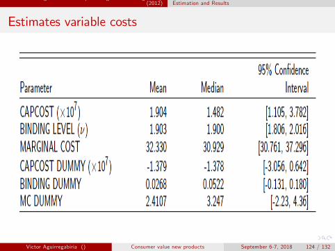
Victor Aguirregabiria () Consumer value new products September 6-7, 2018 116 / 132
Environmental regulation and adoption of green technologies: Ryan(2012) Model
Costs of Capacity Investment
• Investment costs
ICimt = I {iimt > 0}(
θ(+)0 + θ
(+)1 ∗ iimt + θ
(+)2 ∗ i2imt
)+I {iimt < 0}
(θ(−)0 + θ
(−)1 ∗ iimt + θ
(−)2 ∗ i2imt
)
Victor Aguirregabiria () Consumer value new products September 6-7, 2018 117 / 132
Environmental regulation and adoption of green technologies: Ryan(2012) Model