j ourna l homepage: www.e lsev ie r.com/ locate /powtec
Empirical description of flow parameters in eccentric flow inside a silo model
Irena Sielamowicz a,⁎,1, Michał Czech b,2, Tomasz A. Kowalewski c,3
a Białystok Technical University, Civil Engineering Department, 15-351 Bialystok, Wiejska 45 E, Polandb Białystok Technical University, Mechanical Department, 15-351 Bialystok, Wiejska 45 C, Polandc Institute of Fundamental Technological Research, Polish Academy of Sciences, 02-106 Warsaw, Pawinskiego 5B, Poland
Article history:Received 12 November 2008Received in revised form 3 December 2009Accepted 4 December 2009Available online 11 December 2009
Keywords:MethodologyEmpirical analysisDPIV techniqueEccentric granular flowDischarge on the rightVertical modelPlexiglasVelocityThe modified Gauss type functionch functionMultiple regression
The paper presents the methodology of empirical description and statistical analysis of velocity profiles thatwere depicted by the Digital Particle Image Velocimetry technique (DPIV). Experimental runs were recordedby the high resolution camera in the model with vertical walls. Here we analyze the eccentric discharge withthe outlet located in the bottom close to the right vertical wall of the model. On the base of the experimentalresults we present an empirical analysis of velocities and calculation of the flow rate in two proposeddescriptions of the flow. Velocity functions were presented by the exponential function (the modified Gausstype), by the multiple regression and by the ch function. Also the flow rate was calculated for two presenteddescriptions. Empirical calculations of the stagnant zone boundary was also presented using the readingsfrom velocity profiles.
In this paper the methodology of empirical description of velocities,flow rate and stagnant zone boundary on the base of registered velocityfields in eccentric filling and discharge in 2D silo model is presented. Inpractice even tiny eccentricity of filling or discharge processesmay leadto quite an unexpected behaviour of the structure. During asymmetricalprocesses, flow patterns and wall stresses may be quite different. It istherefore crucial to identify flow patterns developed in the materialduring eccentricfilling or discharge, and to determineboth theflow rateand wall stresses occurring under such state of loads. The issuesmentioned above are closely related to the flow pattern. Measuring andpredicting thepattern offlowingmaterial duringdischargewere carriedout by Cundall and Strack [16], Nedderman and Tüzün [26], Tüzün andNedderman [44], Haussler and Eibl [19], Runesson and Nilsson [33],
Rotter et al. [31]. However, investigation and prediction of the complexflow patterns especially during eccentric discharge still remain achallenge.
2. Literature review
International Standards usually relate to axial symmetric states ofstresses and even avoid defining discharge pressures andflowpatternsbecause of continuing uncertainties. In Standard ENV 1991-4 [1], theflow channel geometry and wall pressures under eccentric dischargeare defined. The Polish Standard PN-89/B-03262 [4], titled “Silosyżelbetowe na materiały sypkie. Obliczenia statyczne”, proposes thevalues of increased coefficients of horizontal pressure during eccentricdischarge. There are codes and guides that include eccentric dischargebut they treat it in a different way [2,3,32]. Also a few theoreticalsolutions have been proposed for the design of silos under eccentricdischarge [21,48,29]. The European Standard [1], includes a commenton the eccentricity of the outlet, the definition of the flow channelgeometry and the wall pressure under eccentric discharge. Eccentricfilling is described as a condition inwhich the top of the heap at the topof the stored solids at any stage of the filling process is not located onthe vertical centreline of the silo. Eccentric discharge is described as aflow pattern in the stored solid arising from moving solid beingasymmetrically distributed relative to the vertical centreline of thesilo. This normally arises as a result of an eccentrically located outlet
382 I. Sielamowicz et al. / Powder Technology 198 (2010) 381–394
but can be caused by other asymmetrical phenomena which are notclearly defined. Calculations for flow channel geometry are requiredfor only one size offlowchannel contactwith thewall,which should bedetermined for ΘC=35°. Other methods of predicting flow channeldimensions may also be used. Wall pressures under eccentricdischarge are defined as the pressure on the vertical zone. Thepressure depends on the distance “z” below the equivalent solidsurface and the frictional traction on the wall at level “z”. So far a fewapproaches have been developed for the design of bins under eccentricdischarge [6,29] or by Wood [48]. The issue of eccentricity has alsobeen found to be one of major causes of hopper failures, given byCarson [9]. Eccentricity of the flow to the silo axis causes the pressurepatterns to become much more complex than in centric cases. In thefield of silo investigations three main issues are analyzed: pressuresunder eccentric discharge, flow patterns and stagnant zone bound-aries. Works on eccentric discharge have been published for manyyears and a few researchers have dealt with this complicated problem.Anon [5] presented eccentric discharge silo loads and wall loads as afunction of discharge rate. Thompson et al. [42]measuredwall loads ina corrugated model grain bin when unloaded eccentrically and theeffect of eccentric unloading in a model bin for different unloadingrates. Pokrant and Britton [28] investigated the effect of eccentricitydraw off and flow rate in a model grain bin. Kamiński [22,23]investigated ways of discharge in silo. Hampe and Kamiński [18]analyzed wall pressures under eccentric discharge. Haydl [20]investigated eccentric discharge and the calculation of bendingmoments in circular silos. Theymade an experimental study of certaineffects of the interaction in the full-scale silo between the reinforcedconcrete silo walls and a free flowingmedium. Safarian andHarris [34]dealt with post-tensioned circular silos for modern industry andpresented irregularities of pressure intensity caused by flowproblems,eccentric discharge, or multiple discharge openings. Rotter et al. [30]discussed experiments with buckling failure problems in which thewall stresses were directly induced by stored solids. De Clercq [15]studiedflowpatterns in a silowith concentric and eccentric outlet, andalso a steel silo with two types of outlets and its susceptibility tobuckling. He found that a thin-walled silo with concentric outlet tendsto be well behaved, and whereas the other one with eccentric outletwas susceptible to buckling and collapse. Itwas also stated that none ofthe existing theories adequately addressed the issue of buckling ofeccentrically-emptied silos. Blight [7] investigated the behaviour of
Fig. 1. Eccentric flow of flax seed: filling from the left and discharge from
two steel silos under eccentric discharge. Borcz et al. [8] presentedexperimental results of pressure measurements in the wall in a full-scale silo under eccentric discharge. Shalouf and Kobielak [35]analyzed eccentric discharge in silos and reduction of the dynamicflow pressures in grain silo by using discharge tubes. Ayuga et al. [6]investigated discharge and the eccentricity of the hopper influence onsilo wall pressures. Molenda et al. [25] presented investigations on binloads by both central and eccentric filling and discharge of grains in amodel of silo. In the analysis, Chou et al. [13] using the kinematicmodel, proposed by Nedderman and Tüzün [26], constructed aboundary-value problem. The results consist of measurements ofcircumferential shell wall deformation for various load histories as afunction given service cycles: filling and discharge — centrally andeccentrically. Chou et al. [13] investigated granular flow in a two-dimensional flat-bottomed hopperwith eccentric discharge.Wójcik etal. [47] presented numerical analysis of wall pressures in silos withconcentric and eccentric hoppers. Chou et al. [12] made someexperiments in a two-dimensionalflat-bottomedmodel and identifiedflow patterns and stresses on the wall during centric and eccentricdischarge. The flowing material was recorded using a digitalcamcorder and the normal and shear stresses were measured usingpressure gauges. Chou and Hsu [14] measured experimentally theheights of the stagnant zones for two kinds of granular materials afterhopper eccentric and centric discharge. Guaita et al. [17] applied FEMmodelling in the analysis of influence of hopper eccentricity on wallpressures. In the proposed model the distribution of plastic areasaccording to eccentricity was analyzed. Song and Teng [39] analyzedthe results in FEM of a buckling strength of steel silo subject to code-specified pressures for eccentric discharge with the wall loadspredicted by four codes where the pressure asymmetry wasdetermined by local pressure increases or reductions and describedby the authors as patch loads. Nübel and Huang [27] presented a studyof localized deformation pattern in granular materials, investigatingshear localizations in granular materials numerically, with the use of aCosserat continuum approach, and compared the obtained results toexperimental data. Tejchman [40,41] also presented a numericalCosserat approach to the behaviour of granular medium in a silo.
The latest paper on the flow pattern measurement however, in afull-scale silo not in a model, was presented by Chen et al. [10]. Onecan find a long list of references concerning investigation of eccentricdischarge there.
the right, a) flow mode formed in the model, b) velocity contours.
Table 1Values of the symbols given in formula (2).
Parameters i=0 i=1 i=2
Ai 3.679 −0.062143 0.000803132Bi 0.065893 0.0081573 −0.000165805Ci −0.10255 0.0035087 −0.000031846
383I. Sielamowicz et al. / Powder Technology 198 (2010) 381–394
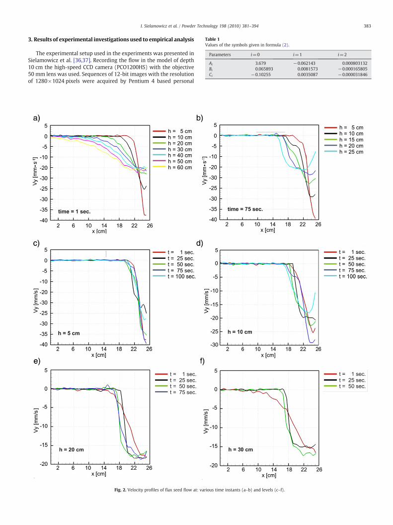
3. Results of experimental investigations used to empirical analysis
The experimental setup used in the experiments was presented inSielamowicz et al. [36,37]. Recording the flow in the model of depth10 cm the high-speed CCD camera (PCO1200HS) with the objective50 mm lens was used. Sequences of 12-bit images with the resolutionof 1280×1024 pixels were acquired by Pentium 4 based personal
Fig. 2. Velocity profiles of flax seed flow at: various time instants (a–b) and levels (c–f).
Table 2Values of coefficients ai in formula (3).
a0 a1 a2 a3 a4 a5 a6 a7 a8 R coefficient of correlation
384 I. Sielamowicz et al. / Powder Technology 198 (2010) 381–394
computer using IEEE1394 interface. The system allowed to acquire upto 1000 images at time interval of 1.5 ms (667 fps). The velocity fieldwas evaluated for triplets of images using the DPIV based on theOptical Flow technique, Quenot et al. [50]. Dense velocity fields withvectors for each pixel of the image were obtained and used for furtherevaluation of the velocity profiles, velocity contours and streamlines.The term “streamline” is defined as a direction of the flow of differentparticles at the same time. Intrinsic resolution of the PIV technique islimited by the size of the area of interest that is used in the applicationof the cross correlation algorithmbetween subsequent images and thisis generally one order of magnitude larger than a single pixel. AnOptical Flow technique based on the use of Dynamic Programming[Quenot et al. [50]] has been applied to Particle ImageVelocimetry thusyielding a significant increase in the accuracy and spatial resolution ofthe velocity field. A velocity vector is obtained for every pixel of theimage and typical for classical PIV constrains are removed. Calibrationcarried out for synthetic sequences of images shows that the accuracyof measured displacement is about 0.5 pixel/frame for tested two-image sequences and 0.2 pixel/frame for four-image sequences.
Table 3Parameters A, B and C in formula (4), the 1st regression.
Slominski et al. [38] presented a detailed description of PIV techniquewith its advantages and disadvantages. The aim of the presentinvestigation is to explore the possibility of using the Optical Flowtechnique based on PIV inmeasuring granularmaterial flow velocity. Inthis paper we apply the Optical Flow technique DPIV to investigatedynamic behaviour of granular material during discharge and measureflow profiles, velocity distributions, vector fields in plane flow hopperswith eccentric filling and discharge. In order to evaluate velocity longsequences of 100–400 images were taken at variable time intervalscovering thewhole discharge time. In granularmaterialflowoneusuallyvisualizes a track of individual particles, not necessarily coinciding withthe streamline. Such trackswere obtained by Choi et al. [11], whoused ahigh-speed imaging technique to trace the position of single particles ingranular materials. Velocity profiles obtained that way for the flow ofgranular material inside a quasi-two-bottomed silo were smooth andfree of shock-like discontinuities. In contrast, the DPIV technique usedhere produces velocity field for the full interrogation area, and this canbe used to predict the natural track of individual particles.
4. Theoretical description of velocities
We present here the methodology of theoretical analysis ofvelocities in asymmetric flow of flax seed in the model with verticaland smooth walls with outlet located close to the right wall. Weconsider the case discussed in Fig. 1 where the flow mode is alsopresented. Themodel has the depth of 5 cm. Properties of the granularmaterial used in the experiment: angle of wall friction againstPlexiglas φw=26o, angle of internal friction φe=25o, Young modulusE=6.11 MPa, granular material density deposited through a pipewith zero free-fall ρb=746 kg/m3 at 1 kPa and 747 kg/m3 at 8 kPa.
Fig. 2 presents selected velocity profiles obtained for the case offilling made from the left and with discharge outlet located near theright wall. The readings taken from the velocity profiles are presentedin Tables 1–7 published in Appendix.
Statistical analysis of the experimental results with application ofthe values given in Tables 1–7 (published in Appendix)was done. Theconfidence intervals for the averages were determined for theanalyzed levels and are listed in Tables 8–13 published in Appendix
Fig. 3. Distributions of parameters A, B and C (points) and their empirical descriptions(solid lines).
385I. Sielamowicz et al. / Powder Technology 198 (2010) 381–394
[46]. The averages were calculated using the sums of the columns inTables 1–6. In the calculations the flow time was not taken intoaccount. In this analysis there are no readings that were removedfrom the data set.
4.1. Description of velocities by the exponential function (generalized,the Gauss type)
At the beginning of the analysis the vertical velocity component Vy
was depended on two factors: the distance x — the location of themeasurement points and also on the various heights z. The type of thefunction applied in the empirical description of vertical velocity Vy
calculated in millimetres per second was proposed as the following:
Vy = eA + Bx + Cx2 ð1Þ
where parameters A, B and C were determined by the least squaresmethod (the first regression), presented in the form of points in Fig. 3.The solid lines show the empirical description of these parameters atvarious analyzed levels.
Parameters A, B and Cwere depended on the height z in the modelaccording to formula (2). Analyzing the distribution of parameters A,B and C we can expect the second regression results to be less agreedwith the experimental results (cf. Fig. 4). Thus, calculating the secondregression, the shape of the function to describe velocity Vy by themultiple regression was determined:
A = A0 + A1z + A2z2
B = B0 + B1z + B2z2
C = C0 + C1z + C2z2:
ð2Þ
Parameters Ai, Bi, and Ci for i=0, 1, 2 were obtained by the leastsquares method using formula (2) and are listed in Table 1.
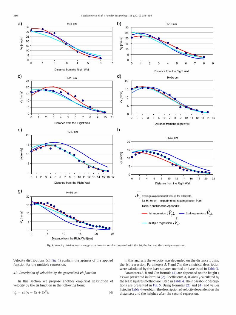
On the basis of formulas (1) and (2) and the values listed inTable 1, velocity distributions were drawn. Fig. 4 presents thecomparison of the average experimental results
PVy expwith empirical
values Vyempir after the 1st regression (depending the velocity onthe distance from the symmetry axis x), after the 2nd regressionˆVy empir, depending the velocity both on the distance x and on the
height z and after the multiple regressionˆVy that is discussed in the
next section.
4.2. Description of velocities by the multiple regression
Applying the 1st and the 2nd regression, the description of verticalvelocity was assumed in the form of the following function:
and x denotes the distance from the left wall, z — is the height of theanalyzed level in themodel, measured in centimetres. The coefficientsa1 where i=0, 1…8 were calculated by the least squares method, andare listed in Table 2. We define the calculations accurately using themultiple regression. There is a possibility to determine the parametersby the nonlinear regression, that would define the description a littlemore accurately.
On the basis of formula (3) and data listed in Table 2, the values of
vertical velocityˆVy were calculated. Three approaches of describing
the velocity in the model presented above are shown in Fig. 4. Thepoints relate to the average values of experimentalmeasurements andthe solid lines represent the functional descriptions of velocity after
the 1st (VyÞ, the 2nd ( ˆVy) and the multiple regression (ˆVy).
It should be stated that there is a problem to find a proper form ofthe function that would describe velocity in the model but the type ofthe function given in formulas (1) and (2) describes the distribution ofvelocity quite well, especially in determining the parameters by themultiple regression. We have also found the best description ofvelocities for the lowest levels at H=5 cm and H=10 cm. The higherthe level is located the higher regression should be applied to describethe velocities. But it is not a rule. This is changing at the middle levels.
Fig. 4. Velocity distributions: average experimental results compared with the 1st, the 2nd and the multiple regression.
386 I. Sielamowicz et al. / Powder Technology 198 (2010) 381–394
Velocity distributions (cf. Fig. 4) confirm the aptness of the appliedfunction for the multiple regression.
4.3. Description of velocities by the generalized ch function
In this section we propose another empirical description ofvelocity by the ch function in the following form:
Vy = ch ðA + Bx + Cx2Þ: ð4Þ
In this analysis the velocity was depended on the distance x usingthe 1st regression. Parameters A, B and C in the empirical descriptionwere calculated by the least squares method and are listed in Table 3.
Parameters A, B and C in formula (4) are depended on the height zas was presented in formula (2). Coefficients Ai, Bi and Ci calculated bythe least squares method are listed in Table 4. Their parabolic descrip-tions are presented in Fig. 5. Using formulas (2) and (4) and valueslisted in Table 4we obtain the description of velocity dependent on thedistance x and the height z after the second regression.
Fig. 5. Distribution of parameters A, B and C.
387I. Sielamowicz et al. / Powder Technology 198 (2010) 381–394
On the basis of the 1st and 2nd regressions we assumed thevertical velocity in the form:
Parameters a1 where i=0,1,2…8 were calculated by the leastsquares method, and listed in Table 5. Variables x1, x2, x3, x4, x5, x6, x7,and x8 were applied like in formula (3).
Applying the approaches presented above we show the verticalvelocity distributions in Fig. 6. Description of velocities by the ch
function also proved that at the higher levels the best agreement ofthe experimental and empirical results was obtained by the first andthe multiple regression. The second regression was only needed topredict the type of the function to describe velocity.
4.4. Verification of the accuracy of the applied descriptions
We also verified the accuracy of the applied descriptions. In Table 6the sums of the squares of the differences of velocities in three appliedregressionsby theGaussdescriptionandby the ch functionarepresented.
As it is seen the best description of velocities was found using thech function because the sum of the sums of the squares is lower, bothin the used regressions and at the analyzed levels.
4.5. Flow rate
The flow rate Q was calculated for two presented descriptions ofvelocities. In the solution given by the Gauss exponential function theflow rate was calculated according to the following formula:
Q = ∫xn
0
eA + Bx + Cx2dx ð6Þ
and the values of Q are listed in Table 7. In formulas (6) and (8) thelimit of integration xn denotes the distance of the last measurementpoint from the right wall taken from the experimental readings forvarious analyzed levels (cf. Tables 1–7 published in Appendix). Theflow rate was described by the following parabolic function:
Q = A1 + B1z + C1z2 ð7Þ
where parameters A1=110.54, B1=−0.20605, and C1=0.26017 werecalculated by the least squares method using the values listed in Table 7.On the basis of parameters A1, B1, and C1, the values of the flow rate Qwere determined and these values were used in calculations of the sumsof the squares of the differences that are also listed in Table 7.
In the description of velocities by the ch function, the flow rate wascalculated according to the formula:
Q = ∫xn
0
chðA + Bx + Cx2Þdx ð8Þ
and the values are listed in Table 7. The limit of integration xn wastaken like in formula (6). The flow rate Q was also described by theparabolic function given in formula (7) and parameters A2=110.18,B2=−0.076199, and C2=0.024345 were determined by the leastsquares method using the values listed in Table 7. On the basis of thevalues of parameters A2, B2, and C2, the values of the flow rate Q werecalculated and used to determine the sums of the squares of thedifferences of velocities that are also listed in Table 7.
In both solutions the parameters Ai, Bi, and Ci for i=1,2, wereintroduced into the analysis after the 1st regression, from Fig. 3 andTable 3, respectively. The best description of the flow rate wasobtained by the Gauss function, because the sum of the sums of thedifferences of velocities given in Table 7 is lower than in the case of thedescription made by the ch function (Fig. 7).
In the two presented cases the calculated values of the flow rateQ·[cm2/s] are almost similar, both in the empiric description (by theparabolic function) and by the integrated values using formulas (6)and (8), respectively. In the region between the levelH=5 cm and thelevel H=10 cm where the flow channel is the narrowest (cf. Fig. 1),the increase of the flow rate reaches approximately the similar values.From this level the increase of theflow rate is rapid. From levelH=20 cmup and higher the increase of the flow rate is not constant. As a result ofdifferentiating formula (7) we obtain the linear increment of the velocityof the flow rate at different levels. The difference of the flow rate reaches0.352 [cm2/s] between levelsH=20 cmandH=30 cmand 1.053 [cm2/s]
Fig. 6. Vertical velocity descriptions by the three applied methods.
Table 7Values of the flow rate (integrated).
Level H[cm]
xn[cm]
Q [cm2/s] Sums of the squares of differences ∑ðQempir− QÞ2
388 I. Sielamowicz et al. / Powder Technology 198 (2010) 381–394
Fig. 7. Comparison of the flow rate calculated by: a) the function of the Gauss type,b) the ch function.
Fig. 8. Range of the stagnant zone boundary at the analyzed instants of the flow.
389I. Sielamowicz et al. / Powder Technology 198 (2010) 381–394
between levels H=30 cm and H=40 cm, respectively. But higher thanH=40 cm the flow rate increases more rapidly because the flow channelwidens, thusmorematerialflows into itwithhigher velocity. The increaseof the flow rate between level H=40 cm and H=50 cm is again lowerand reaches 1.303 [cm2/s] and between levelH=50 cm andH=60 cm isalready 4.616 [cm2/s]. The flow channel at levelH=50 cm is sowide thatthe flow rate reached more than 15.0 [cm2/s].
5. Empirical determination of stagnant zone boundary
Basing on the readings listed in Tables 1–7 given in Appendix, thedistances xi (for instance x=2, 3, 4, and 5 cm) were determined fromthe right wall of themodel. And the last four readings of velocities Vy ofnonzero valueswere taken for the analysis. VelocitiesVywere dependedon x by the functions of: the parabolic type Vy=A1+B1x+C1x
2,hyperbolic type Vy = A + B
x, or linear type Vy=a+bx. We searchedthe values x at which Vy=0 (stagnant zone boundary). At first weapplied theparabola of the secondorder to approximate the four chosenexperimental readings of vertical velocityVy. Ifwedonot obtain the zerovalues of velocities in the assumed approximation thenwe should applyanother function to approximate the experimental values of velocitiesVy. From these two functions only one can be chosen for which thecoefficient of correlation has the highest value. The choice of theparabolic function for the first approximation came out from the factthat the more there are constant coefficients in the description of thefunction, the more accurate description should be expected. Here weapproximated values of velocities by the three proposed types of thefunctions and we obtained values x for which Vy=0 (stagnant zoneboundary). Several authors defined the stagnant zone boundary in avarious way: Zhang and Ooi [49] called it as the flow channel boundary(FCB), as the zone in which the particles do not slough off the solidssurface but follow the paths predicted by the kinematic theory all theway to the outlet. The particles located in the surrounding feeding zone
enter the topflow layer and roll down to the central axis and thenfinallymove towards the outlet. Many numerous investigations at measuringand predicting the pattern of material flow during silo discharging havebeen carried out (e.g. [16,26]). Tüzün and Nedderman [43] defined theflow channel boundary as the streamline within which 99% of the totalflow takes place while Watson and Rotter [45] proposed to define theboundarywhere the velocity at each level is 1%of the centre line velocityat that level. In the case of asymmetric flows the maximal velocitiesoccur in various distances from the rightwall of themodel. HenceVy=0was assumed at the stagnant zone boundary. The values of x and theparameters of the proposed functions are given in Table 14 in Appendix.On the basis of these data, the points of the calculated values of x atwhich vertical velocity Vy=0 are shown in Fig. 8.
The regression lines determined on the basis of the data given inTable 14 (Appendix) are also shown in Fig. 8. Theequationsof these lineswere calculated for the height H≥10 cm and they are the following:
� for 1 s of the flow x = 3:58 + 0:3733H; r = 0:990� for 25th s of the flow x = 5:12 + 0:1884H; r = 0:979� for 50th s of the flow x = 7:21 + 0:163H; r = 0:974� for 75th s of the flow x = 9:08 + 0:076H; r = 1:
ð9Þ
In the presented analysis we described the distribution of therange of the stagnant zone boundary forming in the flowing materialfrom the level H=10 cm up. For heights H≥10 cm it is possible toapproximate the stagnant zone boundary by the line. This fact isconfirmed by the coefficients of correlation given in formula (9).
6. Conclusions
In the presented empirical analysis of velocities in the flowingmaterial in themodelwith eccentricfilling anddischargeweapplied twotypes of functions to describe velocities. We have found that both thefunction of the generalized Gauss type and the ch function decryptvelocities in dependence on variables x and z, especially calculating theparameters of the empirical functions using the multiple regression.However tofind such type of the function (i.e. to dependvelocity both onx and z)firstwe had to apply two single regressions. Having the values ofthe flow rate shown in Fig. 7a and b, described by 2° parabola we caninvestigate theflowrate at lower levels andbyextrapolating the functionwe canpredict thevalues of theflowrate athigher levels. In thepaperwepresented theway on how to predict the stagnant zone boundary. It wasassumed at the boundary velocity Vy=0. We did not apply the value ofvertical velocity Vy at the boundary equal to 1% of the maximal velocitybecause themaximalvaluesof velocity appear indifferentdistances fromthe lateral wall of themodel. Further work is required to investigate thestagnant zone boundary location in asymmetrical flows.
390 I. Sielamowicz et al. / Powder Technology 198 (2010) 381–394
Acknowledgements
The authors express their deep gratitude to Prof. ZenonMróz of theFundamental Technological Research of Polish Academy of Sciences inWarsaw for all suggestions concerning the analysis of the problempresented in this paper. All experiments in DPIV technique were
Table 2Readings at level H=10 cm.
Time [s] Velocities Vy [mm/s] at the distance from the symmetry axis x [cm
0 1 2 3
1 s 24.0 25.0 22.0 17.025 s 21.0 20.0 19.0 20.050 s 20.0 21.0 23.0 19.075 s 28.0 29.0 29.0 25.0100 s 9.0 11.0 17.0 17.0
Table 1Readings at level H=5 cm.
Time [s] Velocities Vy [mm/s] at the distance from the symmetry axis
0 1 2
1 s 36.0 37.0 30.025 s 23.0 25.0 22.050 s 34.0 35.0 33.075 s 38.0 39.0 32.0100 s 27.0 28.0 25.0
Table 3Readings at level H=20 cm.
Time [s] Velocities Vy [mm/s] at the distance from the symmetry axis x [cm]
performed at the Department of Mechanics and Physics of Fluids atthe Institute of Fundamental Technological Research of PolishAcademy of Sciences inWarsaw. Special thanks direct to Mr SławomirBłoński for providing numerical results in DPIV technique. The paperwas partly prepared under the Rector's Project W/IIB/11/06 and S/WM/2/08.
Appendix A. Empirical analysis of the flow of the flax seed in the model with smooth walls. Discharge from the right
[5] Anon 1985 Reliable Flow of Particulate Solids, EFCE Publication Series (EuropeanFederation of Chemical Engineers), 49.
[6] F. Ayuga, M. Guaita, P.J. Aguado, A. Couto, Discharge and the eccentricity ofthe hopper influence on the silo wall pressures, Journal of Engineering Mechanics127 (10) (2001) 1067–1074.
[7] G.E. Blight, Eccentric discharge of a large coal bin with six outlets, Bulk SolidsHandling 11 (2) (1991) 451–457.
[8] A. Borcz, el Rahim, Hamdy, Abd, Wall pressure measurements in eccentricallydischarged cement silos, Bulk Solids Handling 11 (2) (1991) 469–476.
[9] J.W. Carson, Silo Failures: Casehistories and Lessons Learned, Third Israeli Conferencefor Conveying and Handling of Particulate Solids, Dead Sea Israel, May 2000.
[10] J.F. Chen, J.M. Rotter, J.Y. Ooi, Z. Zhong, Flow patterns measurement in a full scalesilo containing iron ore, Chemical Engineering Science 60 (2005) 3029–3041.
[11] J. Choi, A. Kudrolli, M.Z. Bazant, Velocity profile of granular flow inside silos andhoppers, Journal of Physics: Condensed Matter 17 (2005) S2533–S2548.
[12] C.S. Chou, J.Y. Hsu, Y.D. Lau, Flow patterns and stresses on the wall in a two-dimensional flat-bottomed bin, Journal of Chinese Institute of Engineers,Transactions of the Chinese Institute of Engineers, Series A 26 (4) (2003) 397–408.
[13] C.S. Chou, Y.C. Chuang, J. Smid, S.S. Hsiau, J.T. Kuo, Flow patterns and stresses onthe wall in a moving granular bed with eccentric discharge, Advanced PowderTechnology 13 (1) (2002) 1–13.
[14] C.S. Chou, J.Y. Hsu, Kinematic model for granular flow in a two-dimensional flat-bottomed hopper, Advanced Powder Technology 14 (3) (2003) 313–331.
[15] H. de Clercq, Investigation into Stability of a Silo with Concentric and EccentricDischarge, Civil Engineers in South Africa 32 (3) (1990) 103–107.
[16] P.A. Cundall, O.D.L. Strack, A discrete numerical model for granular assemblies,Geotechnique 29 (1) (1979) 47–65.
[17] J.S. Guaita, A. Couto, F. Ayuga, Numerical simulation of wall pressure during dis-charge of granular material from cylindrical silos with eccentric hoppers, BiosystemEngineering 85 (1) (2003) 101–109.
[18] Hampe E, Kamiński M 1984 Der Einfluss exzentrischer Entleerung auf dieDruckverhealtnisse in Silos, Bautechnik, Jg. 61, 1 H, 73–82, 2 H, 136–142
[19] U. Haussler, J. Eibl, Numerical investigations on discharging silos, Journal ofEngineering Mechanics, Division ASCE 110 (EM6) (1984) 957–971.
[20] H.M. Haydl, Eccentric Discharge in Circular Silos, Proceedings of the Institution ofCivil Engineers 83 (1987) 2.
[21] A.W. Jenike, Denting of circular bins with eccentric draw points, Journal of theStructural Division ASCE 93 (1967) 27–35 ST1.
[22] M.Kamiński, Der Betrieb vonSilosmit exzentrischenAuslauf, Bautechnik Jg. 56 (H. 6)(1979) 203–204.
[23] M. Kamiński, Untersuchungdes Zuckerdruckes in Silos: Tl 2. Exzentrische Entleerung,Zuckerindustrie Jg. 111 (10) (1986) 916–921.
[24] Z. Kotulski, W. Szczepiński, Rachunek błędów dla inżynierów, PWN, (ErrorAnalysis with Applications in Engineering), 2004.
[25] M. Molenda, J. Horabik, S.A. Thompson, I.J. Ross, Bin loads induced by eccentricfilling and discharge of grain, Transactions of the ASAE 45 (3) (2002) 781–785.
[26] R.M. Nedderman, U. Tüzün, A kinematic model for the flow of granular materials,Powder Technology 22 (1979) 243–253.
[27] K. Nübel, W. Huang, A study of localized deformation pattern in granular media,ComputerMethods in AppliedMechanics and Engineering 193 (2004) 2719–2743.
[28] D.K. Pokrant, M.G. Britton, Investigation into the Effects of Eccentric Draw off andFlow rate in Model Grain Bin Studies, Paper-American Society of AgriculturalEngineers (1986) 86–4076.
[29] J.M. Rotter, The Analysis of Steel Bins Subject to Eccentric Discharge, Proc., 2ndInter. Conference on Bulk Materials Storage Handling and Transportation, Ins. ofEng, Wollongong, Australia, July 1986, pp. 264–271.
[30] J.M. Rotter, P.T. Jumikis, S.P. Fleming, S.J. Porter, Experiments on the Buckling ofThin-Walled Model Silo Structures, Research Report—University of Sydney, 1988,p. R570.
[31] J.M. Rotter, J.Y. Ooi, C. Lauder, I. Coker, J.F. Chen, B.G.Dale, A Study of the FlowPatternsin an Industrial Silo, Proceedings RELPOWFLO II, Oslo, August 1993, pp. 517–524.
[32] J.M. Rotter, Guide for the Economic Design of Metal Silos, E&FN Spon, London,1998.
[33] K. Runesson, L. Nilsson, Finite element modelling of the gravitational flow of agranular material, Bulk Solids Handling 6 (5) (1986) 877–884.
[34] S.S. Safarian, E.C. Harris, Post-tensioned circular silos for modern industry, BulkSolids Handling 7 (1987) 2.
[35] F. Shalouf, S. Kobielak, Reduction of the dynamic flow pressure in grain silo byusing discharge tubes, Powder Handling Processing 13 (2001) 1.
[36] I. Sielamowicz, S. Błoński, T.A. Kowalewski, Optical technique DPIV in measure-ments of granularmaterial flow, part 1 of 3— plane hoppers, Chemical EngineeringScience (2005) 589–598.
[37] I Sielamowicz, S Błoński, TA Kowalewski, Optical Technique DPIV in measure-ments of granular material flow, part 2 of 3 – converging hoppers, ChemicalEngineering Science (2006).
[38] C. Slominski, M. Niedostatkiewicz, J. Tejchman, Application of particie imagevelocimetry (PIV) for deformationmeasurement during granular silo flow, PowderTechnology 173 (2007) 1–18.
[39] C.Y. Song, J.G. Teng, Buckling of circular steel silos subject to code-specifiedeccentric discharge pressures, Engineering Structures 25 (2003) 1397–1417.
[40] J. Tejchman, Behaviour of granular medium in a silo — a numerical Cosseratapproach, part 3, Archives of Civil Engineering 1 (1993) 7–28.
[41] J. Tejchman, Modelling of shear localisation and autogenous dynamic effects ingranular bodies, Habilitation Monograph 140 (1997) 1–353 Veroffentlichungendes Institutes für Bodenmechanik und Felsmechanik der Universität Fridericianain Karlsruhe.
[42] S.A. Thompson, J.L. Usry, J.A. Legg, Loads in a model grain bin as affected by variousunloading techniques, Transactions of the ASAE 29 (1986) 2.
[43] U. Tüzün, R.M. Nedderman, Experimental evidence supporting kinematicmodelling of the flow of granular media in the absence of air drag, PowderTechnology 24 (2) (1979) 257–266.
[44] U. Tüzün, R.M. Nedderman, An investigation of the flow boundary during steady-state discharge from a funnel flow bunker, Powder Technology 31 (1) (1982) 27–43.
[45] G.R. Watson, J.M. Rotter, A finite element kinematic analysis of planar granularsolids flow, Chemical Engineering Science 51 (16) (1996) 3967–3978.
[46] W. Volk, Applied Statistics for Engineers, second edition, by Mc Graw-Hill, 1969.[47] M.Wójcik, G.G. Enstad, M. Jecmenica, Numerical calculations of wall pressures and
stresses in steel cylindrical silos with concentric and eccentric hoppers, Journal ofParticulate Science and Technology 21 (3) (2003) 247–258.
[48] J.G.M. Wood, The Analysis of Silo Structures Subject to Eccentric Discharge,Proc.,2nd Int. Conf. on Design of Silos for Strength and Flow, Stratford-upon-Avon,1983, pp. 132–144.
[49] K.F. Zhang, J.Y. Ooi, A kinematic model for solids flow in flat bottomed silos,Geotechnique 48 (4) (1998) 545–553.
[50] G.M. Quenot, J. Pakleza, T.A. Kowalewski, Particle image velocimetry with opticalflow, Experiments in Fluids 25 (1998) 177–189.