Page 1
1
EMULATE deliverable D12: results of model experiments to determine if the
observed relationships in D7 and D11 can be reproduced or can be better resolved
using the longer timescales of the coupled model experiments, and an initial study of
mechanisms and potential predictability.
Hadley Centre (partner 2), UBERN (partner 6) , SU (partner 7), CEA (partner 4)
Adam Scaife1, Jonas Bhend
2, Paul Della-Marta
2, David Fereday
1, Chris Folland
1,
Jeff Knight1, Anders Moberg
3 and Pascal Yiou
4
1- Hadley Centre, Met Office, UK
2- University of Bern, Switzerland
3- University of Stockholm, Sweden
4- Laboratoire des Sciences du Climate et de l’Environment, France
1. Introduction
The role of the oceans and anthropogenic climate change in determining extratropical
atmospheric variability is far from clear. Reproducibility of Atlantic and European climate
anomalies in the 3rd Hadley Centre model (Pope et al. 2000) forced with observed
sea-surface temperature (SST) and climate forcings was therefore a focus of the
EMULATE project.
Here we describe results from numerical models and compare them with observed signals.
We use two ensembles of simulations run specifically for the EMULATE project and made
available to the EMULATE project partners through www.HadC20C.org. We have used a
“natural” forcing ensemble which has boundary forcing from observed sea surface
conditions, volcanic aerosol and solar variability, as well as an “all forcing” ensemble.
This ensemble, in addition to the natural boundary forcings also contains changes in well
mixed greenhouse gases (CO2, CH4, N2O, CFCl3, CF2Cl2), tropospheric ozone and
stratospheric ozone changes since 1975, surface albedo and vegetation changes and
anthropogenic sulphate aerosol changes. We present a summary of our main results on the
prominent modes of climate variability in these simulations. We use a variety of analysis
methods ranging from simple composite analysis, to the application of the new clustering
technique on atmospheric data that was developed earlier in EMULATE and applied to
observational data (deliverable D7, Philipp et al., 2006).
2. Winter North Atlantic Oscillation (NAO) in EMULATE experiments, additional
perturbation experiments and long coupled simulations
Both the natural and all-forcings model ensembles capture the winter NAO as the first
mode of winter interannual variability and winter clusters of observational data show
positive and negative NAO-like clusters. We therefore projected the modelled daily
weather patterns onto the observed clusters (Philipp et al. 2006) by designating each model
day according to its nearest cluster centroid. In the January to February period there are
clusters which correspond to the negative and positive phases of the NAO. Fig.1 shows
Page 2
2
that while these anomalies are not exactly symmetric opposites, they do show similar
characteristics with opposite anomaly centres over the Azores and Iceland.
Figure 1: Cluster centroids corresponding to the winter NAO positive phase (left) and
negative phase (right) in hPa. Upper panels show sea-level pressure anomalies (coloured)
and total sea level pressure (contours), middle panels show observed composite SST
anomalies preceding atmospheric anomalies by 1 month and lower panels show similar
SST anomalies composited using the modelled cluster frequencies for 1871-2002. Crosses
indicate statistical significance at the 90% level.
The modelled interannual variability of the NAO in both the natural and all-forcing
ensembles of simulations, and the modelled NAO index of Azores minus Iceland MSLP
both show reasonable amplitude when compared to the EMULATE sea level pressure
dataset. However, individual year to year variations of the NAO such as the strongly
negative NAO in 1962/63 are not reproduced in the model. There is also a striking absence
of a strong link with SST on multidecadal timescales. Fig.1 shows that a tripole like SST
pattern occurs prior to both the positive and negative phases of the NAO in observations
but that this link is only weakly represented in the model.
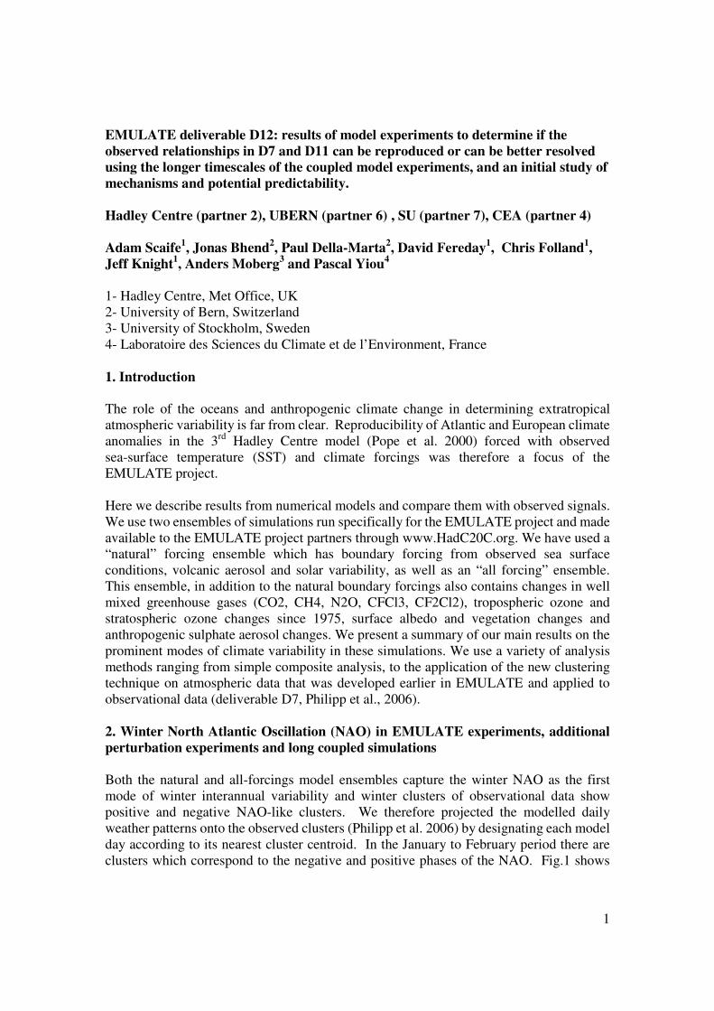
This weak link between SST and the NAO in the EMULATE ensembles is also seen in the
multidecadal trend of the NAO over the latter part of the 20th century. Fig.2 shows that
despite including a comprehensive set of radiative forcings, the observed increase in the
NAO can not be reproduced in our standard GCM simulations.
Page 3
3
1965 1995
Year
Figure 2: Observed and modelled NAO index (hPa) in a set of GCM simulations with all
(anthropogenic and natural) forcings and observed sea-surface temperature and sea-ice.
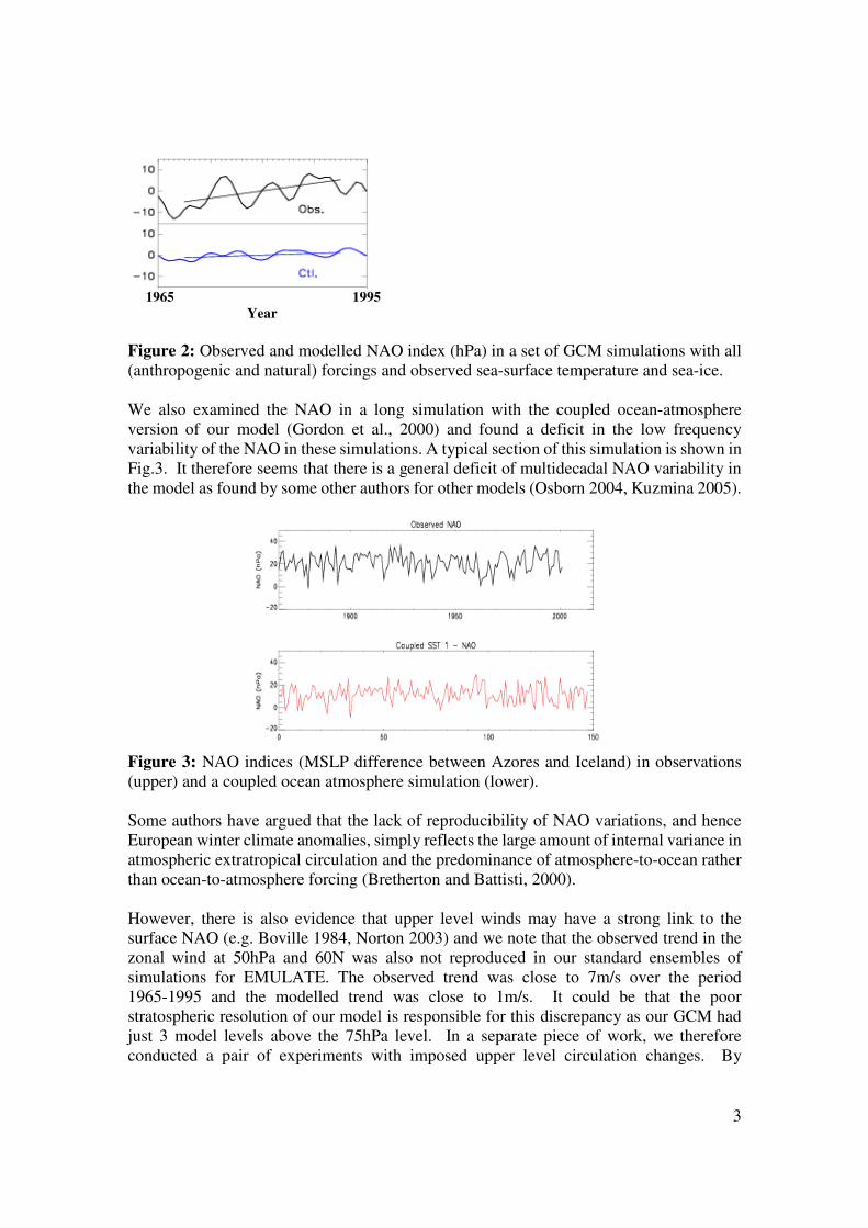
We also examined the NAO in a long simulation with the coupled ocean-atmosphere
version of our model (Gordon et al., 2000) and found a deficit in the low frequency
variability of the NAO in these simulations. A typical section of this simulation is shown in
Fig.3. It therefore seems that there is a general deficit of multidecadal NAO variability in
the model as found by some other authors for other models (Osborn 2004, Kuzmina 2005).
Figure 3: NAO indices (MSLP difference between Azores and Iceland) in observations
(upper) and a coupled ocean atmosphere simulation (lower).
Some authors have argued that the lack of reproducibility of NAO variations, and hence
European winter climate anomalies, simply reflects the large amount of internal variance in
atmospheric extratropical circulation and the predominance of atmosphere-to-ocean rather
than ocean-to-atmosphere forcing (Bretherton and Battisti, 2000).
However, there is also evidence that upper level winds may have a strong link to the
surface NAO (e.g. Boville 1984, Norton 2003) and we note that the observed trend in the
zonal wind at 50hPa and 60N was also not reproduced in our standard ensembles of
simulations for EMULATE. The observed trend was close to 7m/s over the period
1965-1995 and the modelled trend was close to 1m/s. It could be that the poor
stratospheric resolution of our model is responsible for this discrepancy as our GCM had
just 3 model levels above the 75hPa level. In a separate piece of work, we therefore
conducted a pair of experiments with imposed upper level circulation changes. By
Page 4
4
applying a drag on the zonal circulation in the stratosphere of our model which decreased
in magnitude with time we were able to reproduce a trend of 8.5m/s in the winds at 50hPa
and 60N between 1965 and 1995, in reasonable agreement with observations.
A surprising and important finding is that these perturbed simulations also successfully
reproduced the 1965-1995 changes in the winter surface NAO and European surface
climate (Scaife et al., 2005). It therefore seems that predictability of winter European
conditions could in principle be limited by poor simulation of stratospheric conditions.
Additional effects on climate extremes and links with EMULATE work package 4 are
documented below.
5. Summer NAO in EMULATE experiments
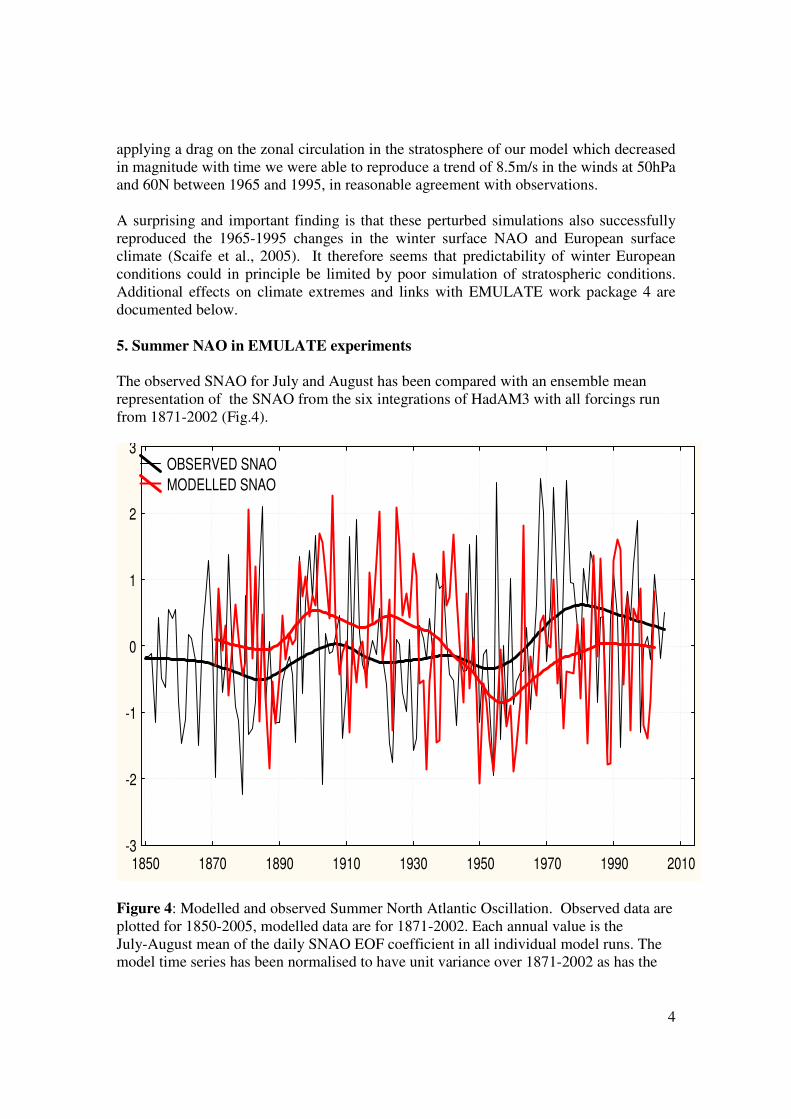
The observed SNAO for July and August has been compared with an ensemble mean
representation of the SNAO from the six integrations of HadAM3 with all forcings run
from 1871-2002 (Fig.4).
1850 1870 1890 1910 1930 1950 1970 1990 2010-3
-2
-1
0
1
2
3 OBSERVED SNAO
MODELLED SNAO
Figure 4: Modelled and observed Summer North Atlantic Oscillation. Observed data are
plotted for 1850-2005, modelled data are for 1871-2002. Each annual value is the
July-August mean of the daily SNAO EOF coefficient in all individual model runs. The
model time series has been normalised to have unit variance over 1871-2002 as has the
Page 5
5
observed time series. Model and observed annually- resolved time series, together with a
smoothed series are based on a locally averaged regression method. This effectively
provides a near bidecadal filter and highlights the low frequency variations.
Concentrating first on the low frequency variability, broadly similar behaviour can be seen
between model and observations with a minimum in the SNAO around 1950 in both the
observations and the model. This peaks in the observations around 1980 and declines
slowly afterwards; a similar peak in the model occurs about a decade later. The late 1960s
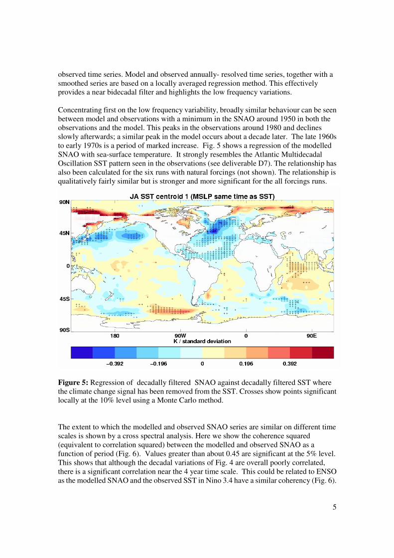
to early 1970s is a period of marked increase. Fig. 5 shows a regression of the modelled
SNAO with sea-surface temperature. It strongly resembles the Atlantic Multidecadal
Oscillation SST pattern seen in the observations (see deliverable D7). The relationship has
also been calculated for the six runs with natural forcings (not shown). The relationship is
qualitatively fairly similar but is stronger and more significant for the all forcings runs.
Figure 5: Regression of decadally filtered SNAO against decadally filtered SST where
the climate change signal has been removed from the SST. Crosses show points significant
locally at the 10% level using a Monte Carlo method.
The extent to which the modelled and observed SNAO series are similar on different time
scales is shown by a cross spectral analysis. Here we show the coherence squared
(equivalent to correlation squared) between the modelled and observed SNAO as a
function of period (Fig. 6). Values greater than about 0.45 are significant at the 5% level.
This shows that although the decadal variations of Fig. 4 are overall poorly correlated,
there is a significant correlation near the 4 year time scale. This could be related to ENSO
as the modelled SNAO and the observed SST in Nino 3.4 have a similar coherency (Fig. 6).
Page 6
6
0 10 20 30 40 50
Period
0.0
0.1
0.2
0.3
0.4
0.5
0.6
0.7
Sq
ua
red
Co
he
ren
cy
0.0
0.1
0.2
0.3
0.4
0.5
0.6
0.7
0 10 20 30 40 50
Period
0.0
0.1
0.2
0.3
0.4
0.5
0.6
0.7
Sq
ua
red
Co
he
ren
cy
0.0
0.1
0.2
0.3
0.4
0.5
0.6
0.7
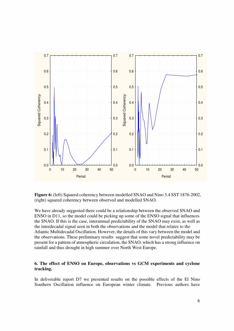
Figure 6: (left) Squared coherency between modelled SNAO and Nino 3.4 SST 1876-2002,
(right) squared coherency between observed and modelled SNAO.
We have already suggested there could be a relationship between the observed SNAO and
ENSO in D11, so the model could be picking up some of the ENSO signal that influences
the SNAO. If this is the case, interannual predictability of the SNAO may exist, as well as
the interdecadal signal seen in both the observations and the model that relates to the
Atlantic Multidecadal Oscillation. However, the details of this vary between the model and
the observations. These preliminary results suggest that some novel predictability may be
present for a pattern of atmospheric circulation, the SNAO, which has a strong influence on
rainfall and thus drought in high summer over North West Europe.
6. The effect of ENSO on Europe, observations vs GCM experiments and cyclone
tracking.
In deliverable report D7 we presented results on the possible effects of the El Nino
Southern Oscillation influence on European winter climate. Previous authors have
Page 7
7
attributed the lack of a robust remote response to ENSO to “non-stationarity”, in other
words to sensitivity of the remote response to the epoch chosen (Sutton and Hodson 2003,
Greatbatch et al. 2004). The implication is that changes in the climatological background
conditions on which the remote response to ENSO develops are different in different
epochs and that this affects the remote response. However, this has not been clearly
demonstrated. An alternative hypothesis is that the response may depend on the amplitude
of the ENSO event itself, as different epochs contain different proportions of weak and
strong ENSO events. By carefully compositing the weak and strong El Nino events
together (Toniazzo and Scaife, 2006) we were able to produce a robust pattern of
anomalies over the Atlantic European region as shown in Fig.7.
Figure 7: Composite mean sea level pressure anomalies in weak (left) and strong (right)
ENSO events from the EMULATE MSLP dataset, January-February means are plotted.
Some aspects of the strong ENSO signal are reproduced in the EMULATE ensemble.
Fig.8 shows similar composites of strong and weak events from the model simulations.
Although weaker than the observed signals, the strong ENSO case reproduces the high
pressure anomalies over the Atlantic and low pressure anomalies over Northern Europe.
There is also a tendency towards and extension of high pressure anomaly across the
Atlantic in the strong ENSO case but the weak ENSO anomaly shown in Fig.7 is not well
reproduced. We went on to investigate the response to ENSO in a set of experiments
parallel to the EMULATE ensemble but using SST anomalies corresponding to composite
means of weak and strong ENSO events. We noted that non-linearity could arise through
the amplitude of the SST anomalies or their pattern which is also different between weak
and strong events. Four ensembles of simulations were therefore run, with perturbations to
Pacific SST corresponding to each of the combinations of weak and strong ENSO pattern
and weak and strong ENSO amplitude.
Page 8
8
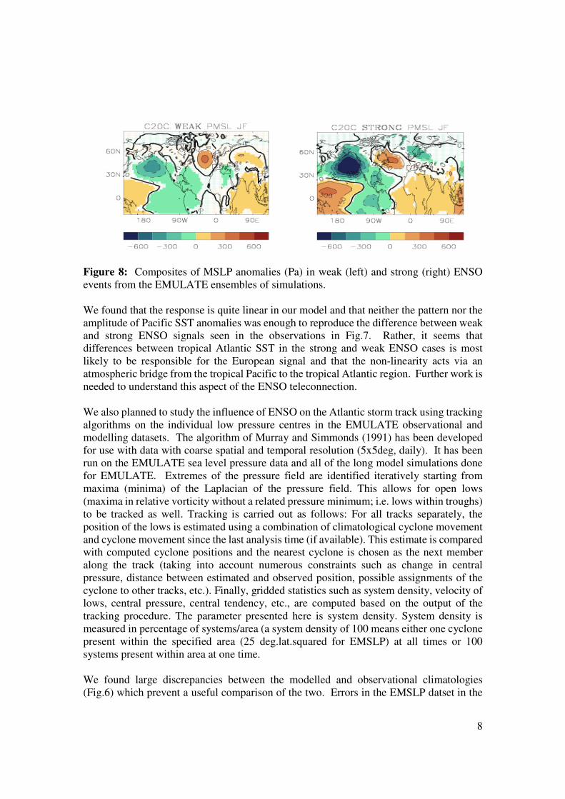
Figure 8: Composites of MSLP anomalies (Pa) in weak (left) and strong (right) ENSO
events from the EMULATE ensembles of simulations.
We found that the response is quite linear in our model and that neither the pattern nor the
amplitude of Pacific SST anomalies was enough to reproduce the difference between weak
and strong ENSO signals seen in the observations in Fig.7. Rather, it seems that
differences between tropical Atlantic SST in the strong and weak ENSO cases is most
likely to be responsible for the European signal and that the non-linearity acts via an
atmospheric bridge from the tropical Pacific to the tropical Atlantic region. Further work is
needed to understand this aspect of the ENSO teleconnection.
We also planned to study the influence of ENSO on the Atlantic storm track using tracking
algorithms on the individual low pressure centres in the EMULATE observational and
modelling datasets. The algorithm of Murray and Simmonds (1991) has been developed
for use with data with coarse spatial and temporal resolution (5x5deg, daily). It has been
run on the EMULATE sea level pressure data and all of the long model simulations done
for EMULATE. Extremes of the pressure field are identified iteratively starting from
maxima (minima) of the Laplacian of the pressure field. This allows for open lows
(maxima in relative vorticity without a related pressure minimum; i.e. lows within troughs)
to be tracked as well. Tracking is carried out as follows: For all tracks separately, the
position of the lows is estimated using a combination of climatological cyclone movement
and cyclone movement since the last analysis time (if available). This estimate is compared
with computed cyclone positions and the nearest cyclone is chosen as the next member
along the track (taking into account numerous constraints such as change in central
pressure, distance between estimated and observed position, possible assignments of the
cyclone to other tracks, etc.). Finally, gridded statistics such as system density, velocity of
lows, central pressure, central tendency, etc., are computed based on the output of the
tracking procedure. The parameter presented here is system density. System density is
measured in percentage of systems/area (a system density of 100 means either one cyclone
present within the specified area (25 deg.lat.squared for EMSLP) at all times or 100
systems present within area at one time.
We found large discrepancies between the modelled and observational climatologies
(Fig.6) which prevent a useful comparison of the two. Errors in the EMSLP datset in the
Page 9
9
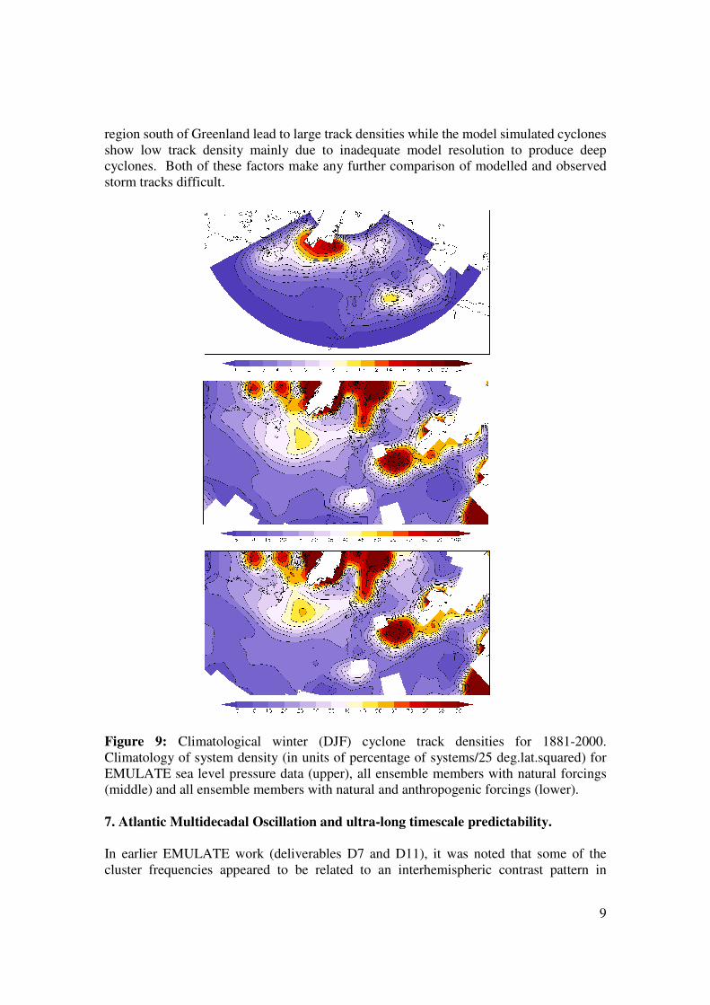
region south of Greenland lead to large track densities while the model simulated cyclones
show low track density mainly due to inadequate model resolution to produce deep
cyclones. Both of these factors make any further comparison of modelled and observed
storm tracks difficult.
Figure 9: Climatological winter (DJF) cyclone track densities for 1881-2000.
Climatology of system density (in units of percentage of systems/25 deg.lat.squared) for
EMULATE sea level pressure data (upper), all ensemble members with natural forcings
(middle) and all ensemble members with natural and anthropogenic forcings (lower).
7. Atlantic Multidecadal Oscillation and ultra-long timescale predictability.
In earlier EMULATE work (deliverables D7 and D11), it was noted that some of the
cluster frequencies appeared to be related to an interhemispheric contrast pattern in
Page 10
10
Atlantic sea surface temperature. This pattern has also been identified as a long lived and
low frequency mode of natural climate variability (Vellinga and Wu, 2004, Knight et al.,
2005) and is termed the Atlantic Multidecadal Oscillation (AMO). This appeared to be
most robust in summer but it also suggested that the analysis ought to be extended to longer
simulations and then to be re-examined in other seasons of the year. To do this we have
examined a multicentury simulation with the coupled ocean-atmosphere version of our
model (Gordon et al., 2000). We use a method outlined in a separate study (Knight et al.,
2005) to isolate the AMO and we have now examined modelled sea level pressure and
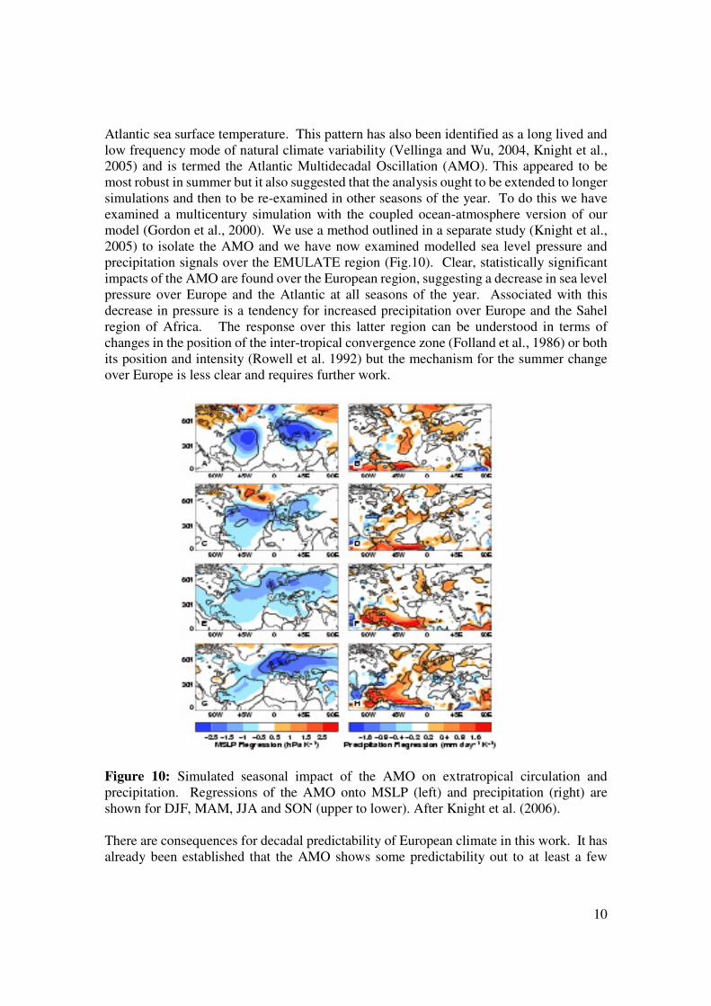
precipitation signals over the EMULATE region (Fig.10). Clear, statistically significant
impacts of the AMO are found over the European region, suggesting a decrease in sea level
pressure over Europe and the Atlantic at all seasons of the year. Associated with this
decrease in pressure is a tendency for increased precipitation over Europe and the Sahel
region of Africa. The response over this latter region can be understood in terms of
changes in the position of the inter-tropical convergence zone (Folland et al., 1986) or both
its position and intensity (Rowell et al. 1992) but the mechanism for the summer change
over Europe is less clear and requires further work.
Figure 10: Simulated seasonal impact of the AMO on extratropical circulation and
precipitation. Regressions of the AMO onto MSLP (left) and precipitation (right) are
shown for DJF, MAM, JJA and SON (upper to lower). After Knight et al. (2006).
There are consequences for decadal predictability of European climate in this work. It has
already been established that the AMO shows some predictability out to at least a few
Page 11
11
decades; because although the oscillation is irregular, it does show coherency on
timescales of up to 50 years (Knight et al., 2005). Given the significant associated signals
in European seasonal mean climate, the AMO therefore represents a new (albeit weak)
potential source of decadal forecasting predictability for Europe.
8. Extremes and links with EMULATE WP4
The modes of variability documented in this report are not only responsible for variability
in the mean climate but also cause variations in climate extremes. In addition to the WP4
analyses of trends in climate extremes we have also examined the response of European
climate extremes to the main mode of extratropical winter variability i.e. the NAO.
As the EMULATE ensemble (like other models) was able to reproduce only a small
fraction of the observed increase in the NAO between the 1960s and 1990s, this ensemble
was used as a “control” for comparison with the simulations described in section 1 in
which upper level circulation changes gave rise to a large increase in the NAO. The result
of this increase in the NAO on heavy rainfall events over Europe is shown in Fig.11.
Figure 11: Changes in the frequency of heavy rainfall events between 1965 and 1995.
Fractional changes in the frequency of 90th
percentile rainfall are shown between 1965 and
1995 in the control EMULATE simulations (left) and simulations with increasing NAO
(right)
Changes in rainfall events in both the control and increasing NAO simulations have a
dipolar structure. This corresponds well with an increase in mean rainfall in northern
Europe and the decrease to the south associated with the NAO (not shown). The changes
are also large, with 75% changes in frequency in areas such as north west Europe. The area
mean values north and south of 42N in Fig.8 are also approximately 5 times larger in the
simulation with increasing NAO than they are in the simulation with only greenhouse
gases and other climate forcings included. In the light of these modelling results, further
evidence for the impact of the NAO on extremes is also being sought using the
observational station datasets produced in WP4. Fig.12 shows one such example where the
relationship between the NAO and the occurrence of European heavy rainfall events is
Page 12
12
verified over the full century timescale. Further examples are being shown in a report by
Mohammad et al. (2006). This provides a clear demonstration that changes in dynamical
modes of variability and not just radiative forcings are crucial in explaining observed
changes in climate extremes on regional scales (Scaife et al. 2006).
Figure 12: Correlations between the frequency of 90th
percentile daily rainfall and the
North Atlantic Oscillation over the 20th
century using EMULATE station data.
9. Conclusions and recommendations for future work
This report describes a range of aspects of climate variability in the EMULATE model
simulations. We have carried out an extensive analysis of our model simulations using
daily cluster analysis and a comprehensive paper is being written on the comparison of
modelled and observed clusters (Fereday et al. 2006).
It turns out that for our model, like many others, even specifying observed global
sea-surface temperatures and other climate forcings is not a sufficient condition to simulate
more than a fraction of the observed increase in the winter NAO (c.f. Cohen et al. 2005).
However, in parallel experiments to those carried out for EMULATE, we have shown that
the increase in the NAO can be reproduced in models if upper level circulation changes are
included. This suggests that future models used to simulate historical European conditions
ought to include an improved representation of the stratosphere and this question will be
answered under continued work under the FP6 EU DYNAMITE project. Current work is
also demonstrating significant potential forecast skill from models on decadal timescales
(Smith et al., 2006) and use of extended models should also be tested for possible benefits
to long range forecasting skill on seasonal to decadal forecast times.
We also tried to characterise the remote effects of ENSO on the Euro-Atlantic region.
Using the long EMULATE MSLP dataset provides a clear advantage for this type of study
over previously available and much shorter records. Further modelling work is required to
attempt to reproduce the observed winter signals, perhaps focussing on tropical Atlantic
SST anomalies. Similarly, higher model resolution may be needed to accurately examine
cyclone statistics and compare these to observations. Modelling experiments with
Page 13
13
localised SST anomalies would also be useful to test the proposed relationship between
ENSO and the NAO in summer.
Finally, there are consequences of this work for interpretation of past climate change
signals over Europe. When annual trends are broken down into seasonal trends, great care
must be taken to properly account for modes of climate variability. For example, the
Atlantic Multidecadal Oscillation can easily project onto regional trends in a variety of
meteorological variables yet we know this is a natural variation of climate. Similarly,
although we can not be sure that the observed change in the winter NAO is not
anthropogenic, recent observations show a downturn in the NAO which is consistent with
natural variability. If the NAO variations are natural in origin then great care must be taken
in interpreting observed trends in both mean and extreme climate events. If, on the other
hand, the NAO variations are anthropogenic in origin, then improved models are needed
which better represent stratospheric processes; in this case we could be underestimating the
rate of winter climate change expected from anthropogenic forcing. Either way,
understanding changes in the primary modes of climate variability is a key question for the
next few years.
References
Boville B.A. 1984: The Influence of the Polar Night Jet on the Tropospheric Circulation in
a GCM. J. Atm. Sci., 41, 1132-1142.
Bretherton C.S. and D.S. Battisti 2000: An interpretation of the results from atmospheric
general circulation models forced by the time history of the observed sea surface
temperature distribution. Geophys. Res. Lett., 27, 767-770.
Cohen J., A. Freie and R.D. Rosen, 2005: The role of boundary conditions in AMIP2
simulations of the NAO. J. Clim., 18, 973-981.
Fereday D.R., J.R. Knight, A.A. Scaife, C.K. Folland and A. Philipp, 2006: Cluster
analysis of North Atlantic/European weather types, J. Clim., in preparation.
Folland, C.K., Parker, D.E. and T.N. Palmer, 1986: Sahel rainfall and worldwide sea
temperatures 1901-85. Nature, 320, 602-607.
Greatbatch R.J., Lu J., Peterson A.K., 2004: Nonstationary impact of ENSO on
Euro-Atlantic winter climate, Geophys. Res. Lett., 31, doi:10.1029/2003GL018542.
Gordon, C., C. Cooper, C.A. Senior, H. Banks, J.M. Gregory, T.C. Johns, J.F.B. Mitchell
and R.A. Wood, 2000: The simulation of SST, sea ice extents and ocean heat transports in
a version of the Hadley Centre coupled model without flux adjustments. Clim. Dyn., 16:
147-168.
Hurrell, J.W. and Folland C.K., 2002: The relationship between tropical Atlantic rainfall
Page 14
14
and the summer circulation over the North Atlantic. CLIVAR Exchanges, 25, 52-54.
Hurrell, J. W., Kushnir, Y., Ottersen G. and M. Visbeck, 2003: An overview of the North
Atlantic Oscillation. In: The North Atlantic Oscillation - climatic significance and
environmental impact. Eds Hurrell, J.W., Kushnir, Y., Ottersen, G. and M Visbeck, pp
1-35. Geophysical Monograph 134, American Geophysical Union, Washington, DC,
pp279.
Knight J.R., R.A. Allen, C.K. Folland, M. Vellinga and M.E. Mann, 2005: A signature of
persistent natural thermohaline circulation anomalies in surface climate. Geophys. Res.
Lett., 32, L20708.
Knight J.R., C.K. Folland and A.A. Scaife, 2006: Climate impacts of the Atlantic
Multidecadal Oscillation, Geophys. Res. Lett., submitted.
Murray, R. and I. Simmonds, 1991. A numerical scheme for tracking cyclone centres from
digital data, Part I: development and operation of the scheme. Australian Meteorological
Magazine, 39, 166.
Murray, R. and I. Simmonds, 1991. A numerical scheme for tracking cyclone centres from
digital data, Part II: application to January and July general circulation model simulations.
Australian Meteorological Magazine, 39, 180.
Norton W.A., 2003: Sensitivity of northern hemisphere surface climate to simulation of the
stratospheric polar vortex. Geophys. Res. Lett., 30, doi:10.1029/2003GL016958 p1627.
Osborn T. J. 2004: Simulating the winter North Atlantic Oscillation: the roles of internal
variability and greenhouse gas forcing. Clim. Dyn., 22, 605-623.
Kuzmina S.I., L. Bengtsson, O.M. Johannessen, H. Drange, L.P. Bobylev and M.W. Miles.
2005: The North Atlantic Oscillation and greenhouse-gas forcing. Geophys. Res. Lett., 32,
L04703.
Mohammad, R., A. Moberg and T. Ansell, 2006: Correlations between indices for
temperature and precipitation extremes in Europe and the leading atmospheric circulation
mode during 1901-2000. Manuscript, contribution to EMULATE D11 and D15, available
on the EMULATE website.
Pope V. D., M. L. Gallani, P. R. Rowntree and R. A. Stratton 2000: The impact of new
physical parametrizations in the Hadley Centre climate model - HadAM3. Clim. Dyn., 16,
123-146.
Rowell, D.P., Folland, C.K., Maskell, K. and J.A. Owen, 1992: Modelling the influence of
global sea surface temperature on the variability and predictability of seasonal Sahel
rainfall. Geophys. Res. Lett., 19, 905-908.
Page 15
15
Scaife A.A., J.R. Knight, G.K. Vallis and C.K. Folland 2005: A stratospheric influence on
the winter NAO and North Atlantic surface climate. Geophys. Res. Let., 32, L18715.
Scaife A.A., L. Alexander, A. Moberg, J.R. Knight, S. Brown and C.K. Folland, 2006:
European weather extremes and the North Atlantioc Oscillation. J. Clim., in preparation.
Sutton, R.T. and D.L.R. Hodson, 2003: Influence of the Oceans on North Atlantic climate
variability 1981-1999, J. Clim.,16, 3296-3313.
Smith, D.M., S. Cusack, A. W. Colman, C. K. Folland and J. M. Murphy, 2006: Improved
surface temperature prediction for the coming decade from a global climate model. Nature,
submitted.
Toniazzo T. and A.A. Scaife, 2006: The effect of non-linearity on winter ENSO
teleconnections over Europe. Geophys. Res. Lett., in preparation.
__________________