Page 1
AAllmmaa MMaatteerr SSttuuddiioorruumm –– UUnniivveerrssiittàà ddii BBoollooggnnaa
DOTTORATO DI RICERCA IN
Ingegneria Civile, Chimica, Ambientale e dei Materiali
Ciclo XXXI
Settore Concorsuale: 08/A2 - Ingegneria sanitaria-ambientale, Ingegneria degli idrocarburi e
fluidi del sottosuolo, della sicurezza e protezione in ambito civile
Settore Scientifico Disciplinare: ING-IND/29 – Ingegneria delle materie prime
ENVIRONMENTAL LIFE-CYCLE BASED METHODS TO
SUPPORT THE TRANSITION TOWARDS CIRCULAR ECONOMY
IN THE AGRI-FOOD SECTOR
Presentata da: Valentina Fantin
Coordinatore Dottorato Supervisore
Prof. Luca Vittuari Prof.ssa Alessandra Bonoli
Co-supervisori
Dott.ssa Patrizia Buttol
(ENEA)
Dott.ssa Serena Righi
Esame finale anno 2019
Page 3
i
Abstract
The holistic approach of Life Cycle Thinking (LCT) can support the transition towards
sustainable production and consumption patterns, in a circular economy approach. The
objective of this dissertation thesis is to critically analyse some peculiar aspects of the
application of environmental life-cycle based methods to the agri-food sector and to
identify opportunities and obstacles of the LCT approach through the testing of some
methods and tools.
The main critical methodological problems of the application of Life Cycle Assessment
(LCA) to agri-food sector were described. In particular, since on-field emissions cannot be
directly measured at a reasonable effort, the analysis was focused on the necessity of using
dispersion models for their estimation. Different models exist but scientific consensus
lacks about the most suitable in terms of reliability and practicability. To test how this
kind of models work and which data are required, PestLCI 2.0 has been applied to an
experimental farm in Northern Italy, and a comprehensive set of pesticide emissions in the
different compartments, which is a relevant input for the inventory phase, has been
obtained. The application has required collecting detailed information about the soil
characteristics, which resulted to affect the outcomes significantly, especially for
groundwater emissions. Since the detailed picture of pesticides emissions is not fully
captured by the current impact assessment methods, further research efforts will be needed
to develop characterisation factors for groundwater emissions, in order to exploit the
potential of PestLCI 2.0.
The analysis of the literature concerning the methodological problems highlighted that
different scientific approaches used to solve the problems might lead to different life cycle
results, thus affecting products comparability, which is important when LCA is used for
calculating and communicating the environmental performance of products. In this
dissertation thesis, the use of LCA for communication purposes was evaluated through the
testing of the Product Environmental Footprint (PEF) method in an Italian Taleggio
cheese production chain, with the aim to evaluate if it fulfils the harmonisation needs for
the calculation and communication of the environmental performance of food and drink
products. Although Product Environmental Footprint Category Rules for dairy products
provide quite detailed guidance for some methodological issues, some other topics would
require additional guidance. The application of the PEF method resulted to be resource-
Page 4
ii
intensive: this aspect could make it difficult to spread the method, especially if the goal is
to involve European Small and Medium Enterprises. In general, the application of the PEF
method could take advantage of the development of simplified supporting tools.
Finally, due to the significant contribution of agricultural sector to water scarcity and
water pollution problems, the Water Footprint (WF) Network method was tested in an
Italian tomato cultivar production with the aim to evaluate strengths and weaknesses. The
study required the collection of a large number of data, some of which obtained from
literature due to lack of primary data. Results highlighted that site-specific data are needed
to increase the results robustness and demonstrated that the effect of the yield may
penalize cultivations with low blue water use, because the model to calculate green water
does not depend on the cultivation intensity, thus leading, ceteris paribus, to higher WF in
extensive cultivations. Though further research will be needed to develop a common
accepted WF method, agri-food companies and public decision makers can take advantage
of this method to support a sustainable water management and the implementation of
green marketing strategies.
Page 5
iii
List of acronyms
AF = Allocation factor
AMD = Availability Minus the Demand
ARPAV = Veneto Regional Agency for Environmental Prevention and Protection
ARPAV = Veneto Regional Agency for Environmental Prevention and Protection
AWARE = Available WAter REmaining for area in a watershed),
B2B = Business to Business
B2C = Business to Consumers
BIB1 = Bibione soil
C = Clay
CAB1 = Caberlotto soil
CAP1 = Capitello soil
CFO1 = Ca' Fornera soil
CMT = Meteorological Centre of Teolo
CON1 = Conche soil
CRL1 = Caorle soil
CTU1 = Ca' Turcata soil
DM = Dry Matter
DNM = Data Needs Matrix
DQR = Data Quality Rating
EEA =European Environment Agency
EF = Environmental Footprint
EMEP = European Monitoring and Evaluation Programme
EPD = Environmental Product Declaration
ET = Evapotranspiration
ILCD = International Reference Life Cycle Data System
Page 6
iv
IPCC = Intergovernmental Panel on Climate Change
IPP = Integrated Product Policy
L = Loam
LCA = Life Cycle Assessment
LCI = Life Cycle Inventory analysis
LCIA = Life cycle impact assessment
LCIA = Life Cycle Impact Assessment
LCT = Life Cycle Thinking
LS = Loamy sand
MEL1 = Casa Scaramello soil
OEF = Organisation Environmental Footprint Organization
PDO = Product Designation of Origin
PEF = Product Environmental Footprint
PEFCR =Product Environmental Footprint Category Rules
QUA1 = Quarto d'Altino soil
S = Sand
SAB1 = Sabbioni soil
SCL = Sandy clay loam
SCO1 = Santa Scolastica soil
SIC = Silty clay
SICL = Silty clay loam
SIL = Silt loam
SL = Sandy loam
SOIL6 = Default soil from PestLCI 2.0 database
SMEs = Small and Medium Enterprises
STU = Soil Typological Units
Page 7
v
TDF1 = Torre di Fine soil
VAD1 = Valcerere Dolfina soil
VAN1 = Vanzo soil
VED1 = Casa Vendramin soil
WF = Water Footprint
WFA = Water Footprint Assessment
WFN = Water Footprint Network
WULCA = Working Group on Water Use in LCA
Page 9
1
Table of Contents
Abstract ................................................................................................................................. i
List of acronyms .................................................................................................................. iii
1 Introduction and objectives ........................................................................................... 9
2 Circular economy ........................................................................................................ 14
2.1 European policies for circular economy ............................................................. 17
3 Circular economy in the agri-food sector ................................................................... 20
3.1 Problems of the linear economic model in the agri-food sector ......................... 20
3.2 Benefits of the circular economy in the agri-food sector ................................... 22
4 Life Cycle based methods to support the transition towards circular economy in the
agri-food sector ................................................................................................................... 24
4.1 Life Cycle Assessment ....................................................................................... 25
4.2 Water Footprint .................................................................................................. 28
4.3 Application of LCA in the agri-food sector: main methodological problems.... 30
4.3.1 Definition of the functional unit ................................................................... 31
4.3.2 System boundaries definition ....................................................................... 34
4.3.3 Allocation procedures ................................................................................... 35
4.3.4 Emission models for pesticides and fertilisers emissions ............................ 39
5 Harmonised LCA guidelines for agri-food production chain ..................................... 45
5.1 ILCD Handbook ................................................................................................. 46
5.2 Envifood Protocol ............................................................................................... 48
5.3 Product Environmental Footprint method .......................................................... 49
6 PestLCI 2.0 sensitivity to soil variations for the evaluation of pesticide distribution in
LCA studies ........................................................................................................................ 53
6.1 Description of PestLCI 2.0 ................................................................................. 54
6.2 Soil and tillage sensitiveness evaluation method ............................................... 59
6.3 Experimental farm description ........................................................................... 60
6.3.1 Climatological data ....................................................................................... 60
6.3.2 Soil data ........................................................................................................ 60
6.3.3 Crop and pesticide data ................................................................................ 67
6.4 Results and Discussion ....................................................................................... 67
Page 10
2
6.4.1 Results of Test 1: comparison among TDF1 and similar soils ..................... 68
6.4.2 Results of Test 2: comparison among TDF1 and different soils .................. 75
6.4.3 Results of Test 3: comparison between TDF1 and Soil6 ............................. 78
6.4.4 Results of Test 4: TDF1 with different types of tillage ................................ 79
6.5 Conclusions ........................................................................................................ 83
7 Product Environmental Footprint Category Rules for dairy products ........................ 86
7.1 Functional unit .................................................................................................... 87
7.2 System boundaries .............................................................................................. 87
7.3 Handling of multi-functionality .......................................................................... 88
7.4 On-farm pesticides and fertilisers emissions and livestock emissions ............... 90
7.5 Water use and related impacts ............................................................................ 92
8 PEF study on Taleggio cheese production .................................................................. 93
8.1 Goal and scope of the study ............................................................................... 93
8.1.1 Goal of the study .......................................................................................... 93
8.1.2 Functional unit and reference flow ............................................................... 93
8.1.3 Description of the life cycle of the analysed product ................................... 94
8.1.4 System boundaries and system boundaries diagram .................................... 95
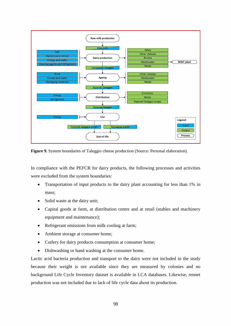
8.1.5 Assumptions and relevant justification ........................................................ 99
8.1.6 Information about the data used and data gaps ............................................ 99
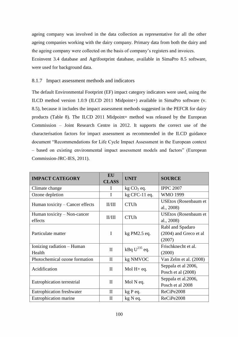
8.1.7 Impact assessment methods and indicators ................................................ 100
8.1.8 Treatment of multi-functionality ................................................................ 101
8.2 Life cycle inventory analysis ............................................................................ 102
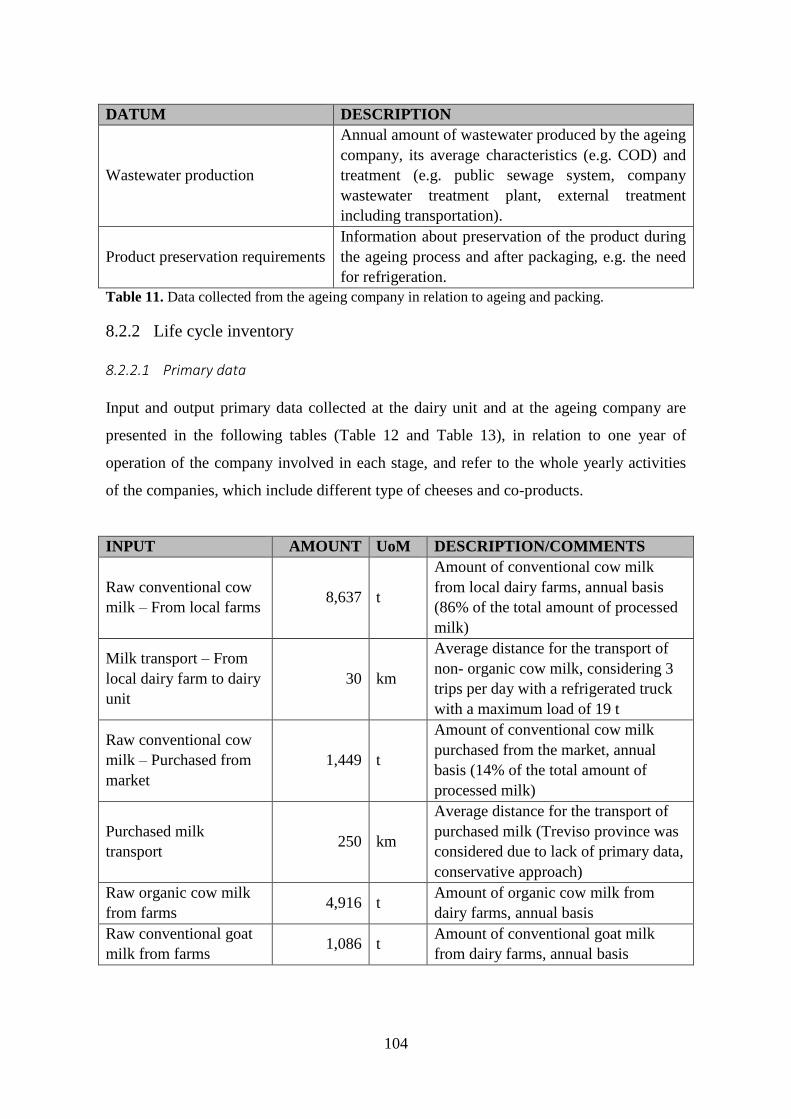
8.2.1 Description and documentation of all the unit processes data collected .... 102
8.2.2 Life cycle inventory .................................................................................... 104
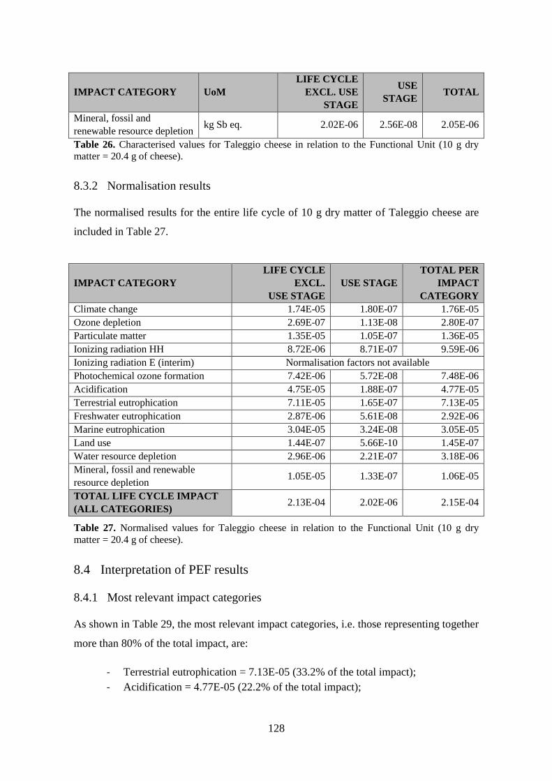
8.3 PEF impact assessment results ......................................................................... 127
8.3.1 Characterization results .............................................................................. 127
8.3.2 Normalisation results .................................................................................. 128
8.4 Interpretation of PEF results ............................................................................. 128
8.4.1 Most relevant impact categories ................................................................. 128
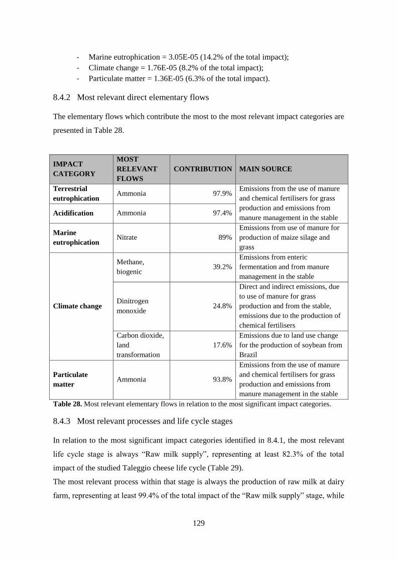
8.4.2 Most relevant direct elementary flows ....................................................... 129
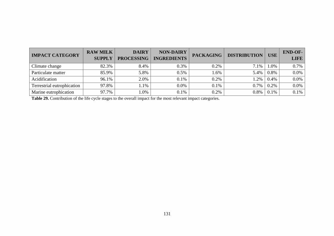
8.4.3 Most relevant processes and life cycle stages ............................................ 129
8.4.4 Overall assessment of data quality ............................................................. 130
Page 11
3
8.5 Conclusions ...................................................................................................... 132
9 Water Footprint Network method and ISO 14046 .................................................... 134
9.1 Water Footprint method by the Water Footprint Network ............................... 134
9.1.1 Setting goals and scope .............................................................................. 135
9.1.2 Water Footprint Accounting: calculation of blue, green and grey WF ...... 136
9.1.3 Water Footprint sustainability assessment ................................................. 139
9.1.4 Water Footprint response formulation........................................................ 142
9.2 The WF by ISO 14046 ..................................................................................... 143
9.2.1 Goal and scope definition ........................................................................... 144
9.2.2 WF inventory analysis ................................................................................ 145
9.2.3 WF impact assessment ............................................................................... 145
9.2.4 Interpretation of results .............................................................................. 147
9.3 Comparison between the WF Network method and ISO 14046 ...................... 147
10 Water Footprint of Italian tomato production ...................................................... 151
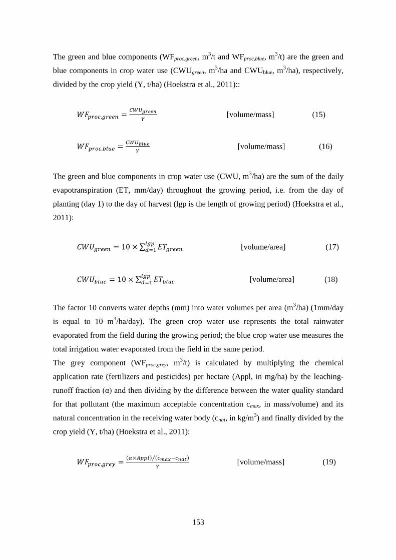
10.1 Calculation of Water Footprint of crop growth ................................................ 152
10.2 Calculation of Green WF ................................................................................. 154
10.3 Calculation of Grey WF ................................................................................... 162
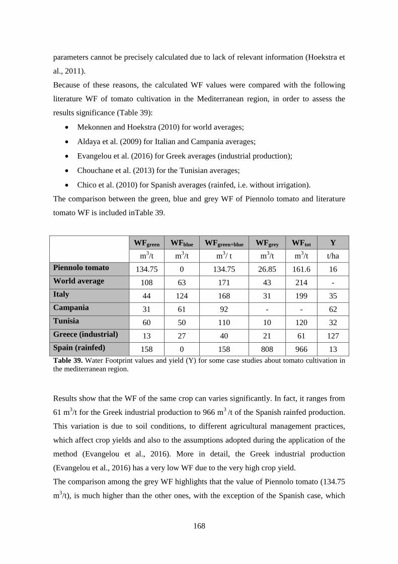
10.4 Results and discussion ...................................................................................... 167
10.5 Conclusions ...................................................................................................... 170
11 Conclusions .......................................................................................................... 173
References ........................................................................................................................ 178
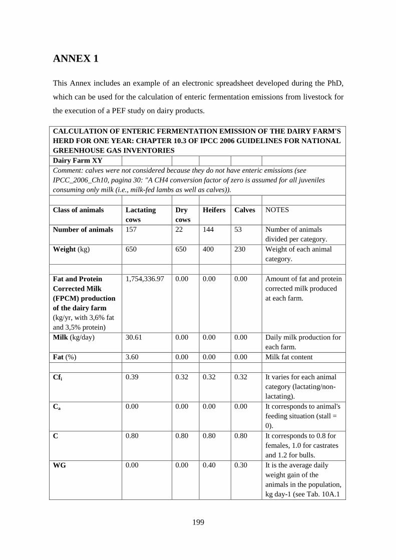
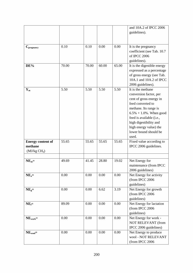
ANNEX 1 ......................................................................................................................... 199
Acknowledgement ............................................................................................................ 202
Page 12
4
List of Figures
Figure 1. Representation of the life cycle phases in the linear and circular economy models
(Source: Personal elaboration adapted from www.riciclanews.it). .................................... 16
Figure 2. Schematic representation of product’s life cycle (Source: ENEA)..................... 25
Figure 3. Four main phases of LCA method (Source: Personal elaboration adapted from
ISO, 2006a). ....................................................................................................................... 27
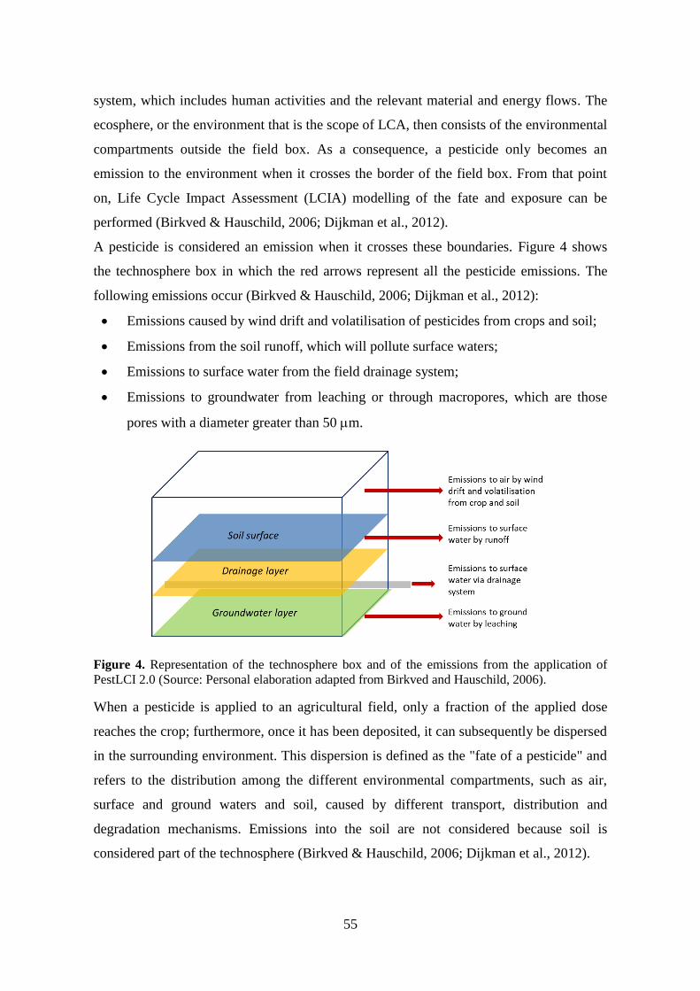
Figure 4. Representation of the technosphere box and of the emissions from the
application of PestLCI 2.0 (Source: Personal elaboration adapted from Birkved and
Hauschild, 2006). ............................................................................................................... 55
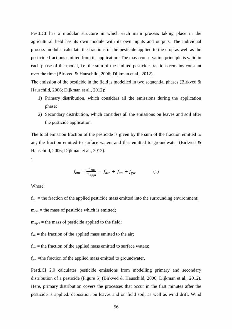
Figure 5. Modular structure of PestLCI 2.0 (Source: Personal elaboration adapted from
Dijkman et al., 2012). ......................................................................................................... 57
Figure 6. Correlation analysis among some soil characteristics and emission fractions of
pesticides. Figures a), b) and c) refer to the first experiment (among similar soils); figures
d), e), f), g), h) and i) refer to the second experiment (among different soils) (Source:
Personal elaboration). ......................................................................................................... 74
Figure 7. Percentage of Terbuthylazine emitted in pre-emergence according to the
different types of tillage (Source: Personal elaboration). ................................................... 82
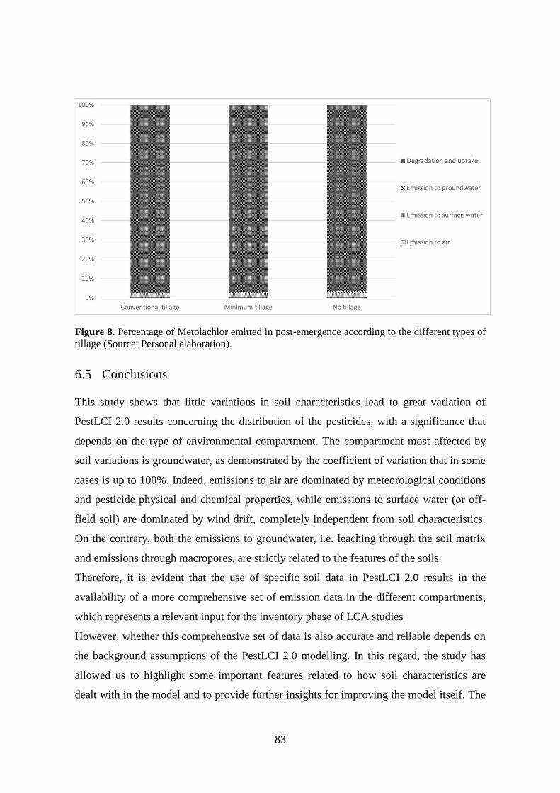
Figure 8. Percentage of Metolachlor emitted in post-emergence according to the different
types of tillage (Source: Personal elaboration). .................................................................. 83
Figure 9. System boundaries of Taleggio cheese production (Source: Personal
elaboration). ........................................................................................................................ 98
Figure 10. Representation of the components of a Water Footprint (Source: Personal
elaboration adapted from Hoekstra et al., 2011). ............................................................. 135
Figure 11. The four phases of the Water Footprint sustainability assessment in a river
basin (Source: Personal elaboration adapted from Hoekstra et al., 2011). ...................... 139
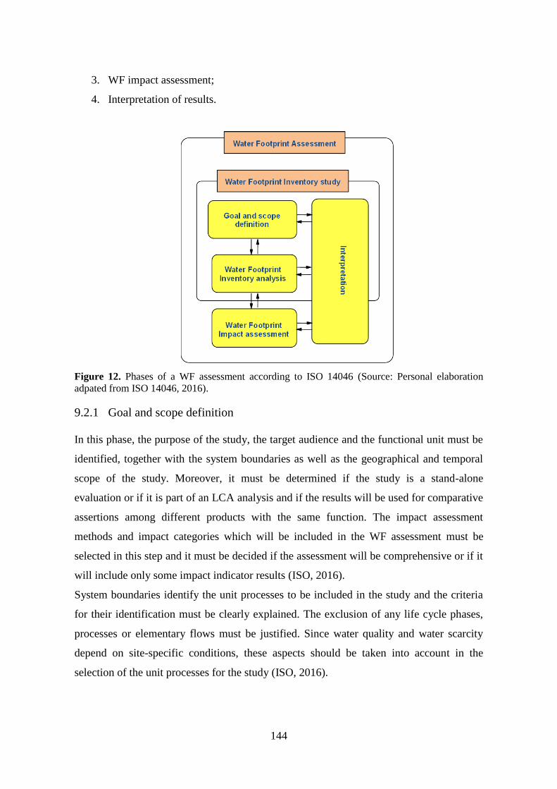
Figure 12. Phases of a WF assessment according to ISO 14046 (Source: Personal
elaboration adpated from ISO 14046, 2016). ................................................................... 144
Figure 13. Comparison between the WFN method and ISO 14046 (Source: Personal
elaboration adapted from Boulay et al., 2013). ................................................................ 150
Figure 14. Climate parameters inserted in CROPWAT software (Source: CROPWAT
software, personal elaboration). ....................................................................................... 156
Figure 15. Rainfall values inserted in CROPWAT (Source: CROPWAT software, personal
elaboration). ...................................................................................................................... 157
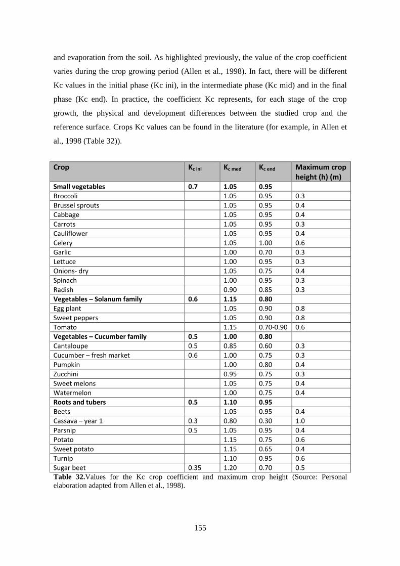
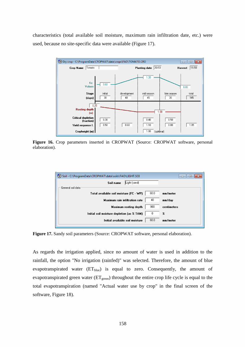
Figure 16. Crop parameters inserted in CROPWAT (Source: CROPWAT software,
personal elaboration). ....................................................................................................... 158
Page 13
5
Figure 17. Sandy soil parameters (Source: CROPWAT software, personal elaboration).
.......................................................................................................................................... 158
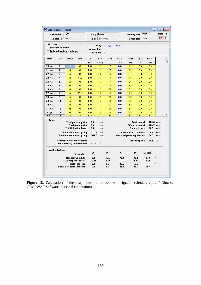
Figure 18. Calculation of the evapotranspiration by the “Irrigation schedule option”
(Source: CROPWAT software, personal elaboration). .................................................... 160
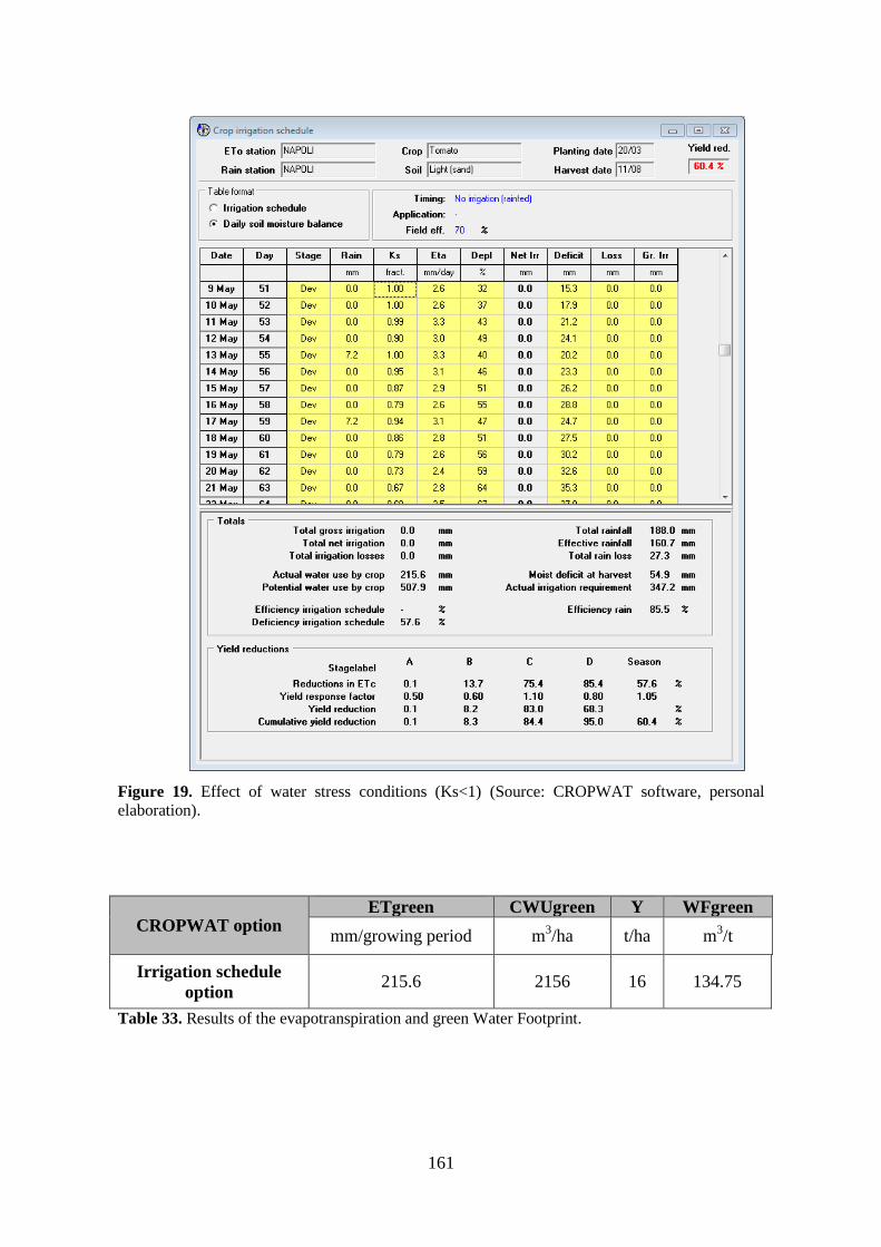
Figure 19. Effect of water stress conditions (Ks<1) (Source: CROPWAT software,
personal elaboration). ....................................................................................................... 161
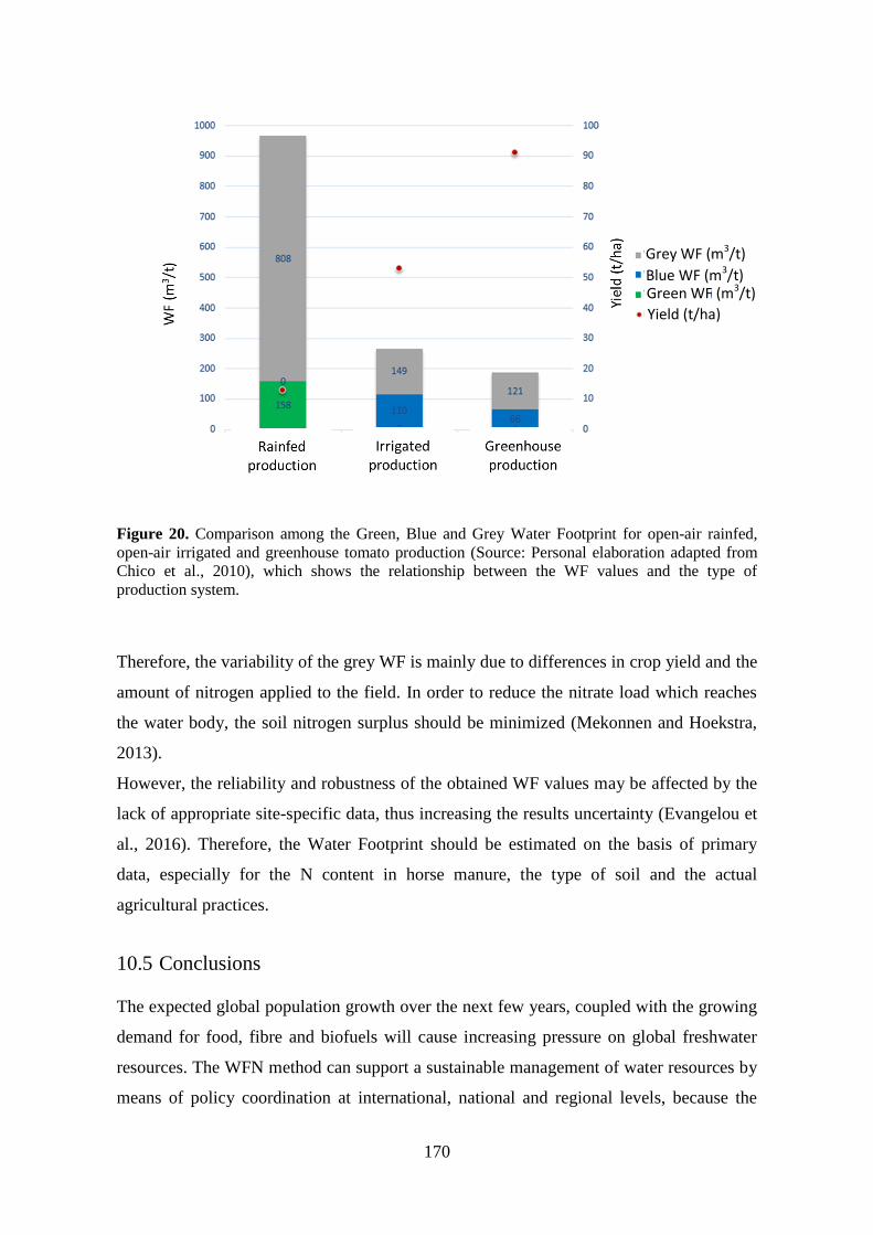
Figure 20. Comparison among the Green, Blue and Grey Water Footprint for open-air
rainfed, open-air irrigated and greenhouse tomato production (Source: Personal
elaboration adapted from Chico et al., 2010), which shows the relationship between the
WF values and the type of production system.................................................................. 170
Page 14
6
List of Tables
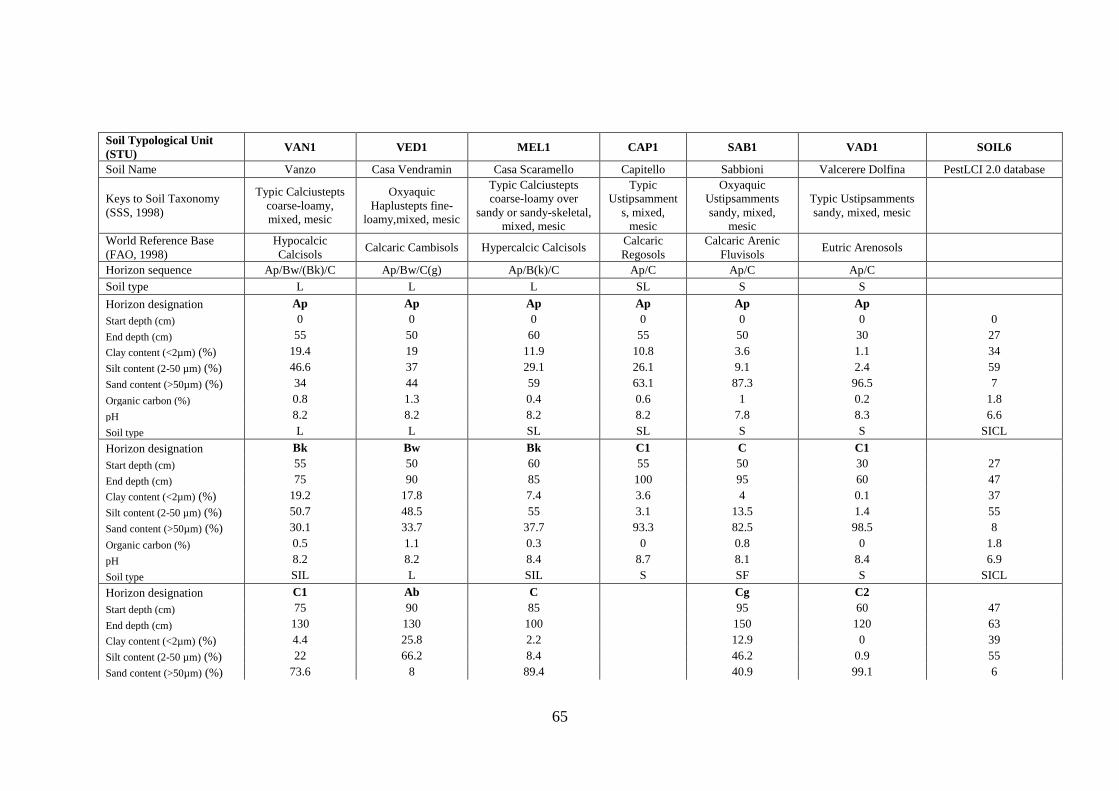
Table 1. Summary characteristics of considered soils (Source: Fantin et al., 2019,
reproduced by permission of Elsevier). .............................................................................. 64
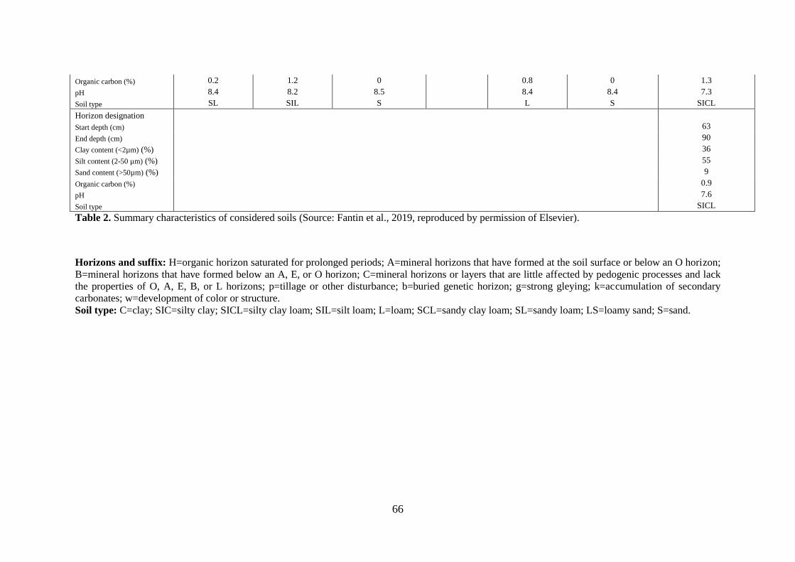
Table 2. Summary characteristics of considered soils (Source: Fantin et al., 2019,
reproduced by permission of Elsevier). .............................................................................. 66
Table 3. Quantity and type of pesticide applied for maize cultivation on the Vallevecchia
experimental farm. (Source: Fantin et al., 2019, reproduced by permission of Elsevier). . 67
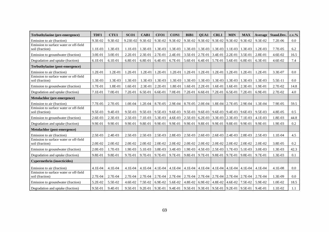
Table 4. Distributions of pesticide among the environmental compartments obtained with
Pest LCI 2.0 model and using site-specific data (TDF1) and those obtained applying data
of soils with similar characteristics. Figures indicate the fraction of pesticide emitted in
each environmental compartment. (Source: Fantin et al., 2019, reproduced by permission
of Elsevier). ........................................................................................................................ 70
Table 5. Distributions of pesticide among the environmental compartments obtained with
Pest LCI 2.0 model using site-specific data (TDF1) and those obtained applying data of
soils with different characteristics. Figures indicate the fraction of pesticide emitted in
each environmental compartment. (Source: Fantin et al., 2019, reproduced by permission
of Elsevier). ........................................................................................................................ 77
Table 6. Results of the application of PestLCI 2.0 model for each active ingredient and for
TDF1 soil and Soil6. Values indicate the fraction of pesticide emitted in each
environmental compartment. (Source: Fantin et al., 2019, reproduced by permission of
Elsevier). ............................................................................................................................. 79
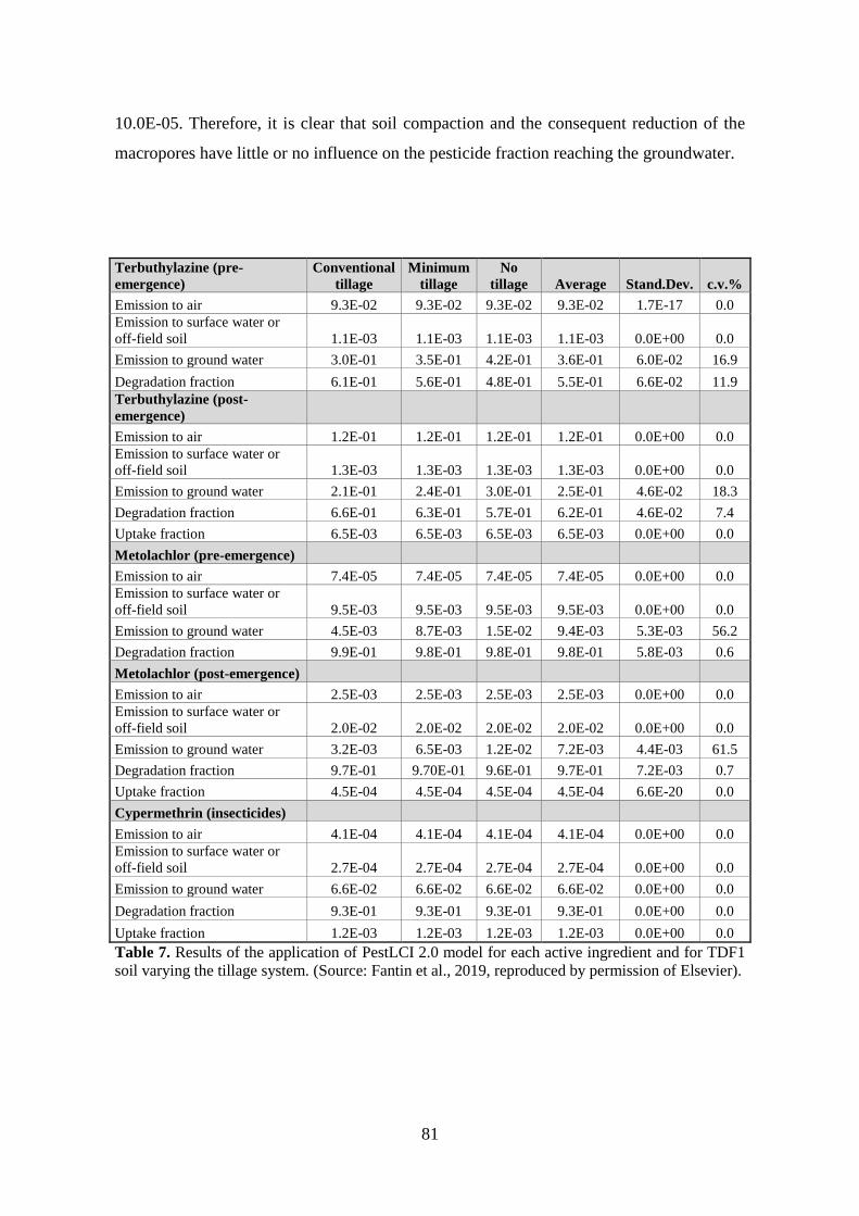
Table 7. Results of the application of PestLCI 2.0 model for each active ingredient and for
TDF1 soil varying the tillage system. (Source: Fantin et al., 2019, reproduced by
permission of Elsevier). ...................................................................................................... 81
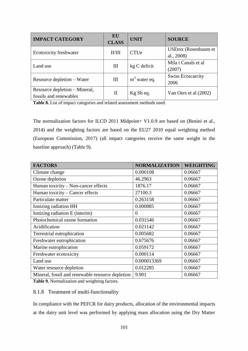
Table 8. List of impact categories and related assessment methods used. ....................... 101
Table 9. Normalization and weighting factors. ................................................................ 101
Table 10. Data collected from the dairy company in relation to unripened Taleggio cheese
production. ........................................................................................................................ 103
Table 11. Data collected from the ageing company in relation to ageing and packing. .. 104
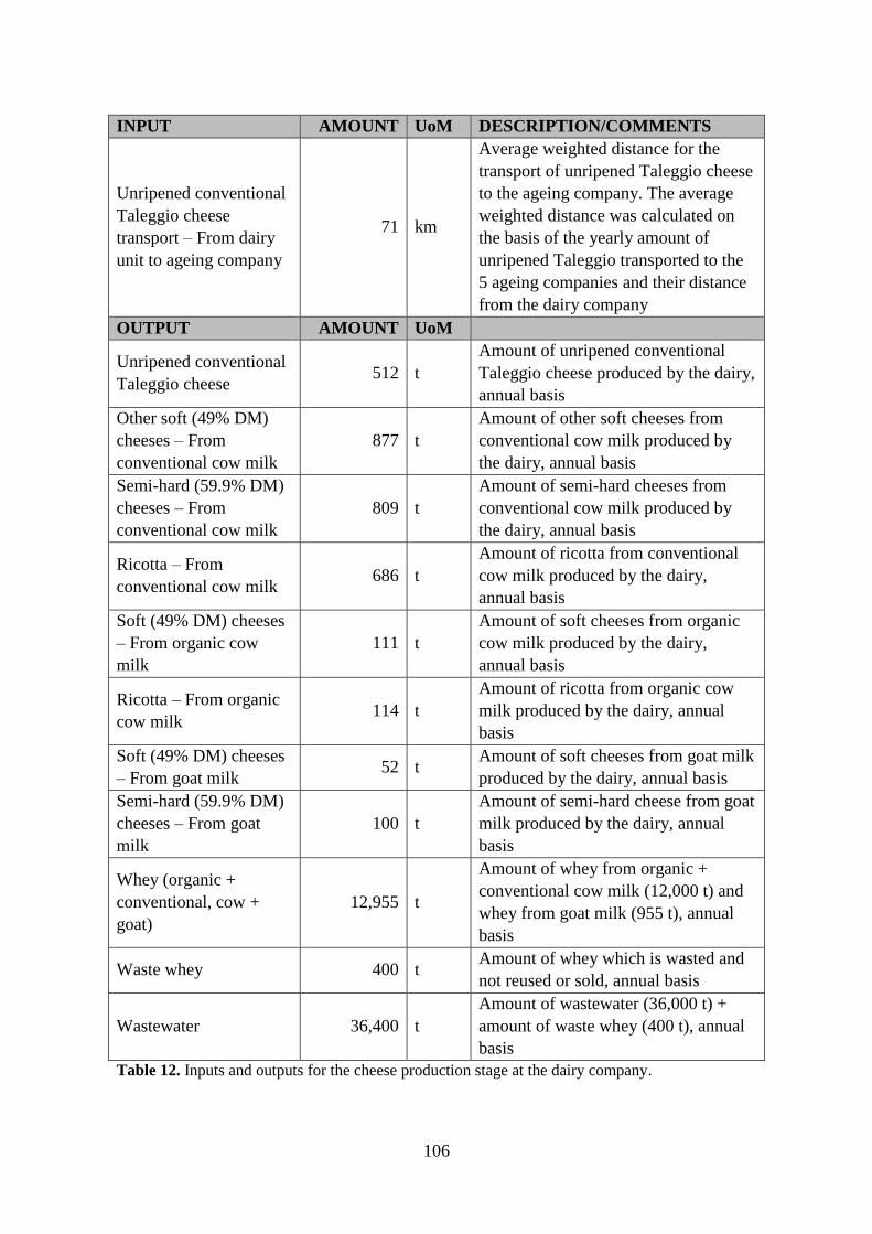
Table 12. Inputs and outputs for the cheese production stage at the dairy company. ...... 106
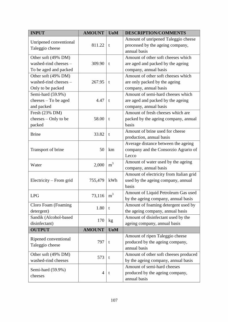
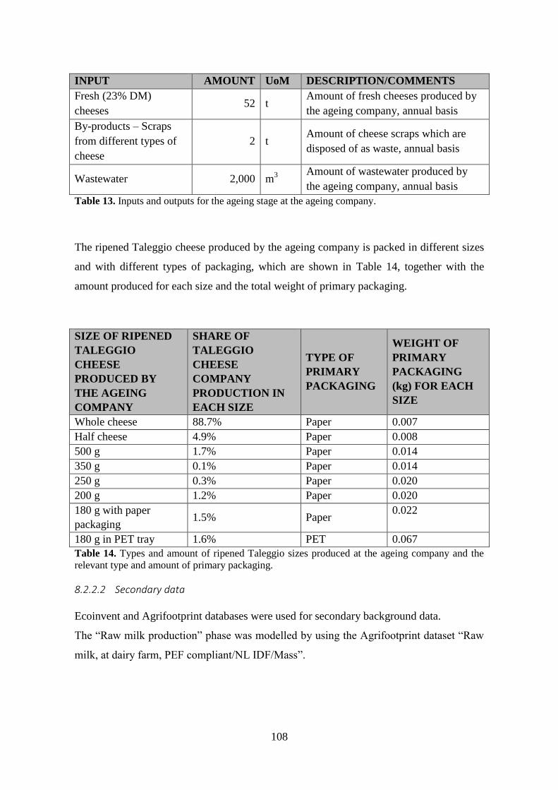
Table 13. Inputs and outputs for the ageing stage at the ageing company. ...................... 108
Table 14. Types and amount of ripened Taleggio sizes produced at the ageing company
and the relevant type and amount of primary packaging. ................................................ 108
Table 15. Inputs and outputs for the cheese production at the dairy company. ............... 110
Page 15
7
Table 16. Allocation factors at the dairy unit for conventional Taleggio cheese production.
.......................................................................................................................................... 111
Table 17. Parameters for the calculation of the average weighted distance for the transport
of unripened Taleggio cheese to the ageing company...................................................... 112
Table 18. Inputs and outputs for the ageing stage at the ageing company. ...................... 114
Table 19. Allocation factors at the ageing company for ripened Taleggio cheese
production. ........................................................................................................................ 114
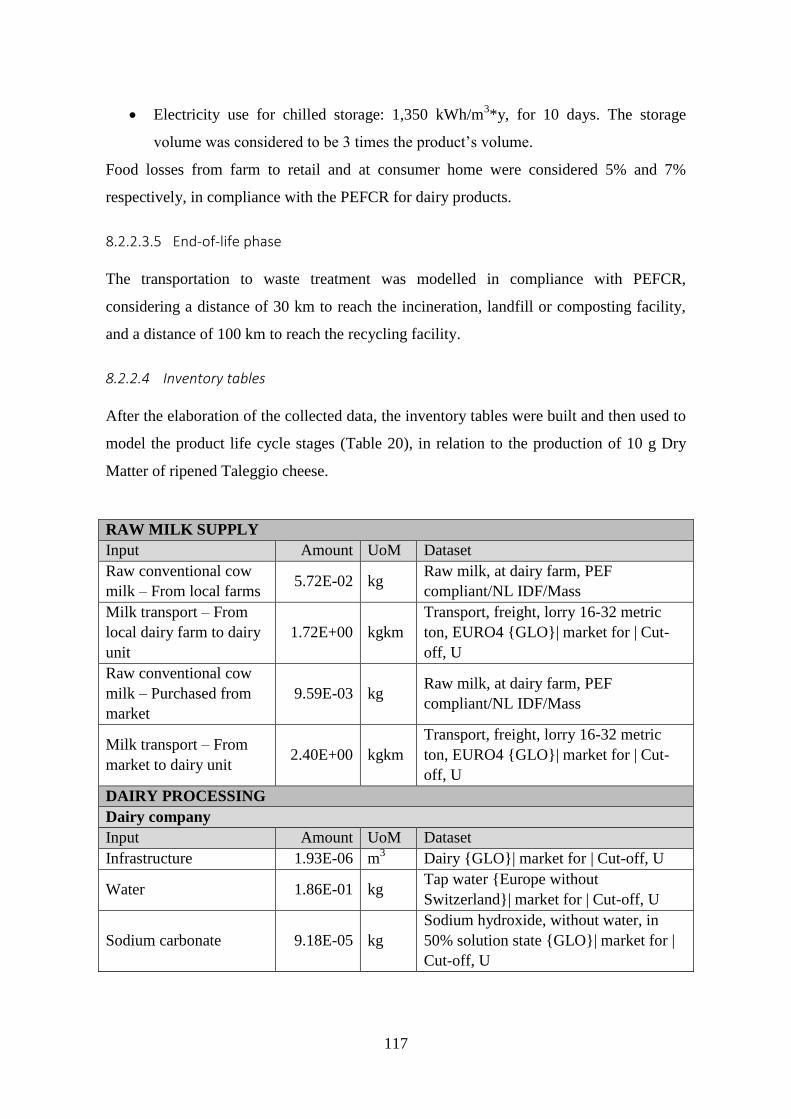
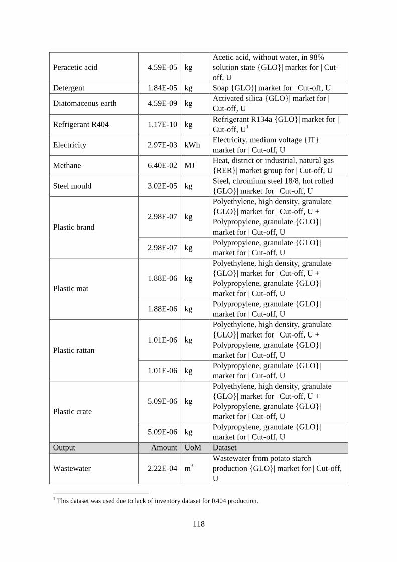
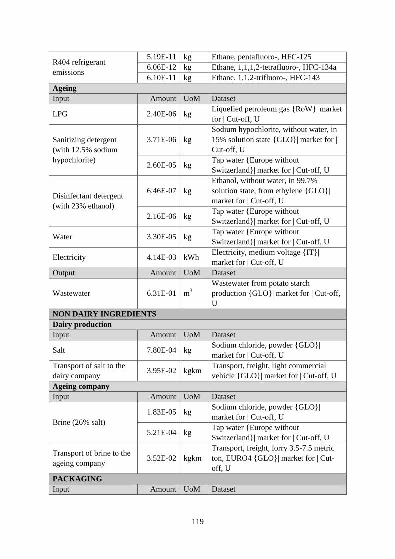
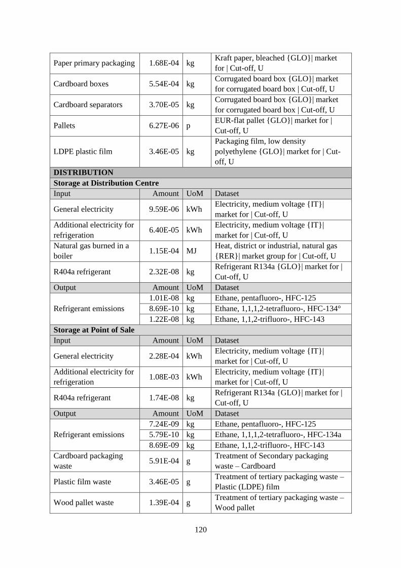
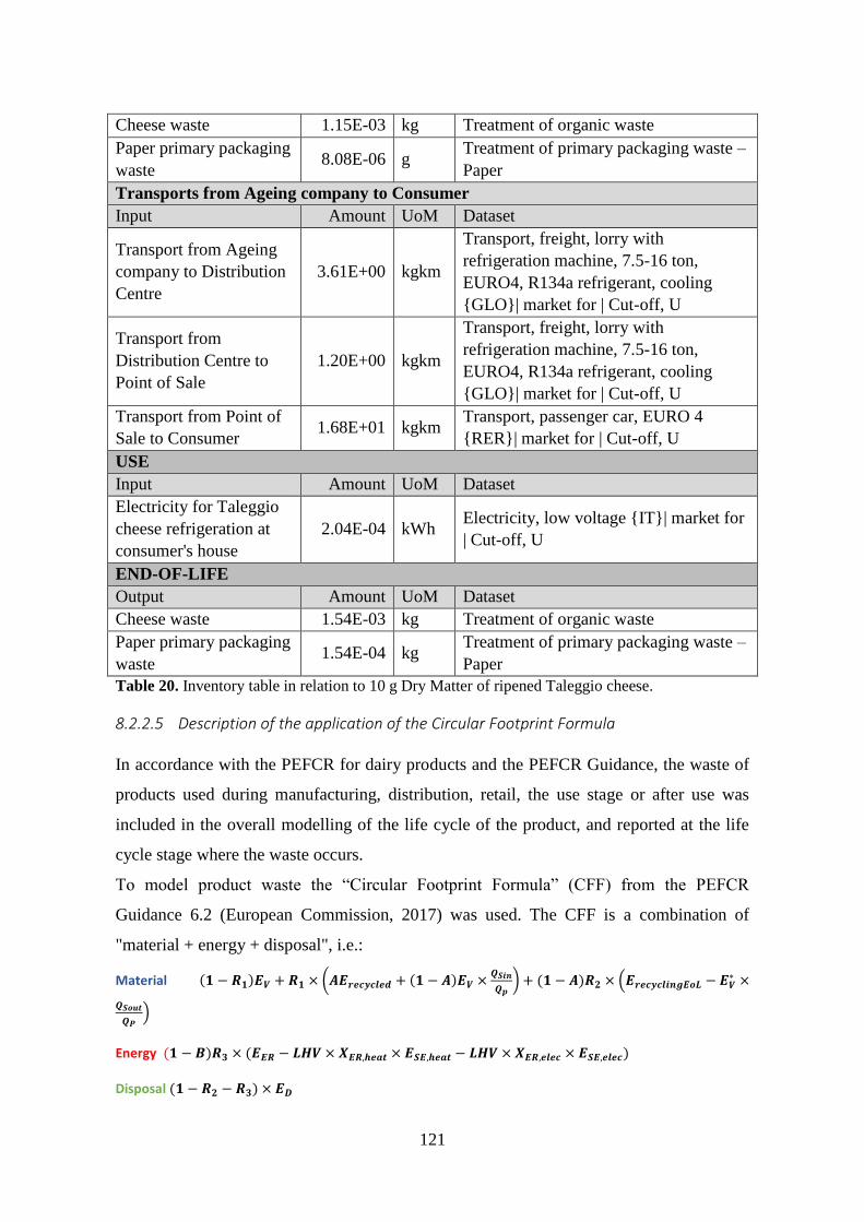
Table 20. Inventory table in relation to 10 g Dry Matter of ripened Taleggio cheese. .... 121
Table 21. Parameters used to model the treatment of organic waste. .............................. 124
Table 22. Parameters used to model the treatment of paper waste. ................................. 125
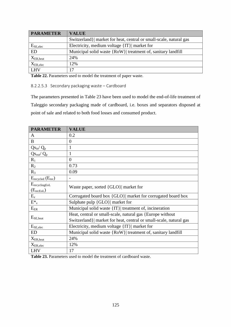
Table 23. Parameters used to model the treatment of cardboard waste. .......................... 125
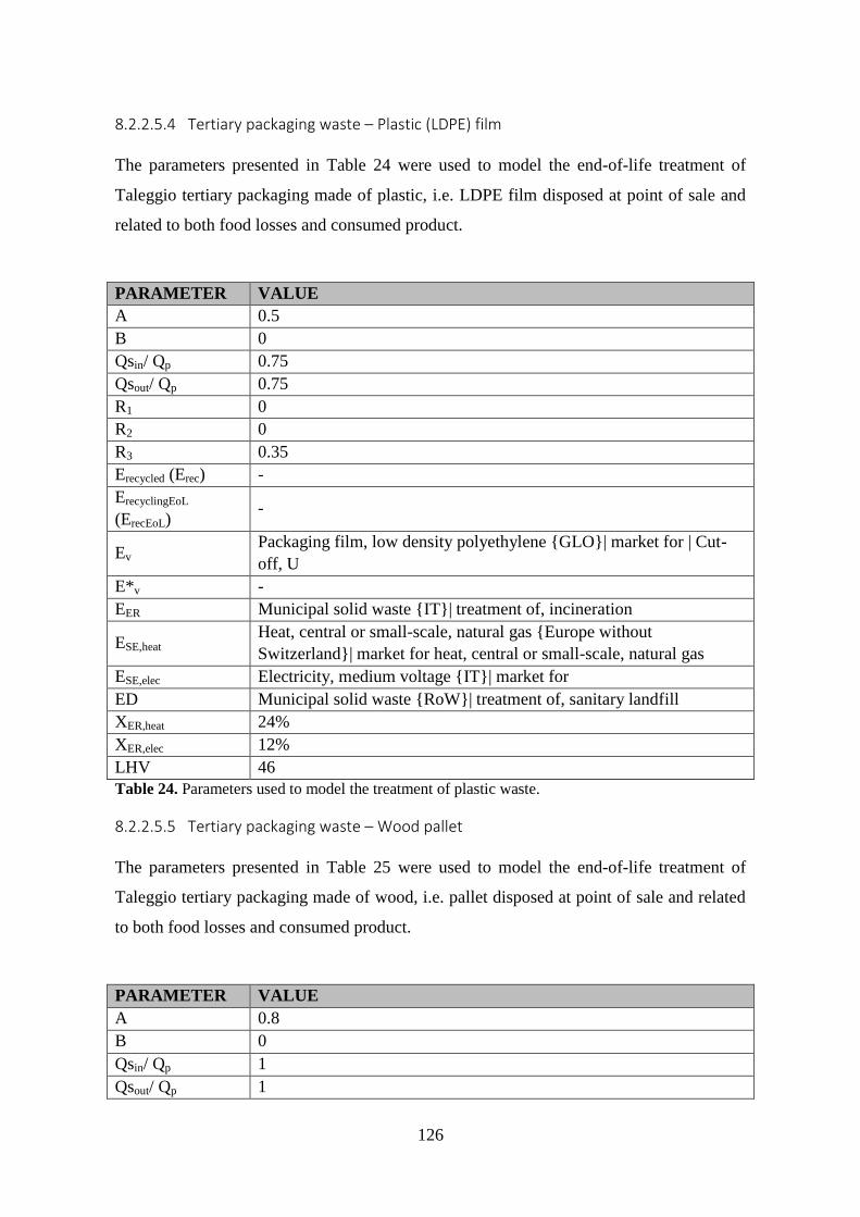
Table 24. Parameters used to model the treatment of plastic waste. ................................ 126
Table 25. Parameters used to model the treatment of wood waste. ................................. 127
Table 26. Characterised values for Taleggio cheese in relation to the Functional Unit (10 g
dry matter = 20.4 g of cheese). ......................................................................................... 128
Table 27. Normalised values for Taleggio cheese in relation to the Functional Unit (10 g
dry matter = 20.4 g of cheese). ......................................................................................... 128
Table 28. Most relevant elementary flows in relation to the most significant impact
categories. ......................................................................................................................... 129
Table 29. Contribution of the life cycle stages to the overall impact for the most relevant
impact categories. ............................................................................................................. 131
Table 30. Considered values for the Data Quality Rating of milk production process. ... 132
Table 31. Primary cultivation data for the production of the PDO Italian tomato. .......... 152
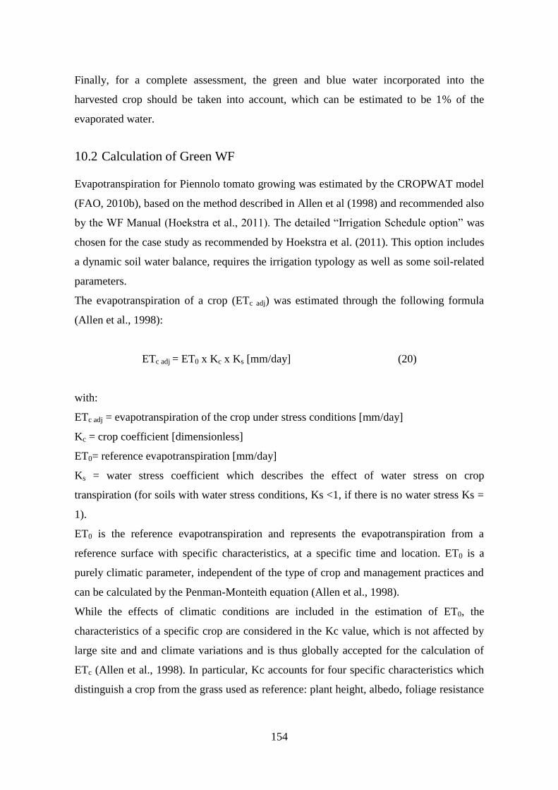
Table 32.Values for the Kc crop coefficient and maximum crop height (Source: Personal
elaboration adapted from Allen et al., 1998). ................................................................... 155
Table 33. Results of the evapotranspiration and green Water Footprint. ......................... 161
Table 34. Minimum, average and maximum values of the leaching-runoff fraction α for
nutrients, metals and pesticides (Source: Personal elaboration adapted from Franke et al.,
2013). ................................................................................................................................ 162
Table 35. Minimum, average and maximum values of the β leaching fraction for nitrogen
and phosphorus (Source: Personal elaboration adapted from Franke et al., 2013). ......... 163
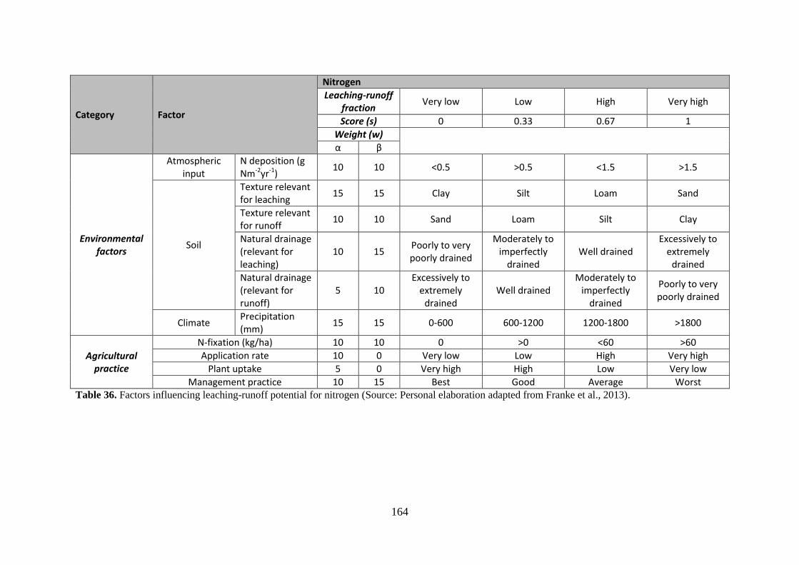
Table 36. Factors influencing leaching-runoff potential for nitrogen (Source: Personal
elaboration adapted from Franke et al., 2013). ................................................................. 164
Table 37. Agricultural management practice questionnaire (Source: Personal elaboration
from Franke et al., 2013). ................................................................................................. 165
Page 16
8
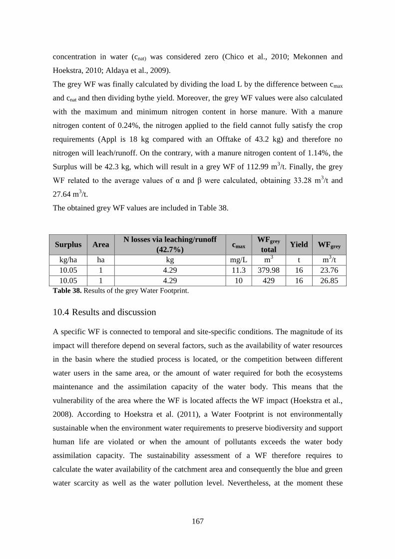
Table 38. Results of the grey Water Footprint. ................................................................ 167
Table 39. Water Footprint values and yield (Y) for some case studies about tomato
cultivation in the mediterranean region. ........................................................................... 168
Page 17
9
1 Introduction and objectives
Agriculture and agri-food sector satisfy one of the most important human needs, i.e.
nutrition and provide significant social and economic values. As regards Italian situation,
the agri-food sector is a priority sector for national economy, due to both its cultural,
social and economic importance and to the peculiarities and specific characteristic of
Italian food and drink products. Nevertheless, the traditional economic model, the so-
called “linear economy”, applied in the last century also in the agri-food sector, as in all
the other manufacturing sectors, and based on the massive exploitation of non-renewable
resources and to the production of significant amount of waste, has become unsustainable
(Ellen MacArthur Foundation, 2013a). In fact, food and drink supply chain has several
important environmental impacts and is the main responsible for the land use change, the
loss of biodiversity, the greenhouse gas emissions and the use of freshwater (European
Commission, 2011). Without appropriate offsetting measures, severe consequences for
both the world population and the environment could occur, such as the lack of food
availability and food security and the almost complete depletion of natural resources.
Because of these reasons, the agri-food sector should move from linear economy models
to circular economy ones, which include sustainable production and consumption patterns
and which could decouple the economic growth from the environmental impacts and the
use of resources (European Commission, 2014a). These topics are included in the most
important international agendas, such as the United Nations’ Global Agenda for
Sustainable Development, which has been signed also by Italian government in 2015, and
the related seventeen Sustainable Development Goals. At European level, the European
Commission’s communication "Closing the loop – An EU Action Plan for Circular
Economy" (COM (2015) 614) represents the most important policy document which
defines circular economy and introduces an action plan for the implementation of a
legislative framework for the development of circular economy measures in all member
states.
However, the transition towards sustainable consumption and production systems in the
agri-food sector, in a circular economy approach, requires the use of robust and scientific
methods which can support sustainability assessment of the overall analysed system for
several sustainability indicators, by appropriately evaluating the consequences of all the
possible circular options, both from an economic, environmental and social point of view.
Page 18
10
Life Cycle Thinking (LCT) approach, which takes into account the whole product’s life
cycle, from the extraction of raw materials, to the product manufacturing, its transport and
distribution, and the final waste disposal can support this transition, because it can be used
for the assessment of the impacts and benefits associated to circular solutions in the agri-
food supply chain, avoiding burden shifting from a phase to another of the life cycle, and
from an environmental compartment to another one.
The objective of this dissertation thesis is to critically analyse some peculiar aspects of the
application of environmental life-cycle based methods and tools to the agri-food sector.
The application of this holistic approach to agri-food production chains allows the
evaluation of their overall ecological performance and supports product development as
well as the implementation of improvement strategies. However, it presents also some
technical and methodological problems that risk to limit a wide use of the approach. In
this work opportunities and obstacles of the approach will be identified through the testing
of some methods and tools and needs for future developments will be discussed.
Among the life-cycle based methods, Life Cycle Assessment (LCA), standardised by the
ISO 14040 series (ISO 2006a, b), is recognised as a strategic and effective tool to evaluate
the potential environmental impacts occurring in the whole product's life cycle as well as
to identify possible areas for improvement. LCA has been used in the recent years to
evaluate the environmental impacts of a wide variety of agri-food products, contributing to
identify the environmental hotspots of the supply chain and the potential improvement
opportunities (Notarnicola et al., 2012). Nevertheless, when applying LCA to food and
drink products, the practitioner has to deal with methodological problems which stem
from the peculiarities and specific characteristics of the agri-food supply chain. In fact,
differently from industrial production systems, agri-food supply chains are characterised
by complex relationships both between inputs (for example nutrients and soil) and outputs
(crops and emissions) and more in general between biological processes and processes of
technological systems, which are difficult to be modelled in LCA studies. In particular, the
inventory phase of LCA studies for food and drink products involves the estimation of on-
field emissions due to the use of fertilisers, pesticides, or emissions from livestock, such as
ruminants’ enteric fermentation, which cannot be directly measured at a reasonable cost
and effort. This is one of the main critical problems in LCA studies of agri-food products,
because these emissions must be calculated by dispersion models, which are based on
several agricultural or livestock site-specific parameters that have to be collected or
Page 19
11
alternatively found in literature (for example the nitrogen content in manure) and which
therefore require specific knowledge in this field. Several literature models are available in
literature, but no scientific consensus still exists on which one should be used.
Among the main critical methodological problems of the application of LCA to agri-food
sector, which will be described in this dissertation thesis, due to the relevance of the
problem for the impact on ecosystems and human health, a focus will be given to the
calculation of on-field emissions due to the use of pesticides at inventory level by
applying the detailed PestLCI 2.0 model (Dijkman et al., 2012) to an experimental farm in
Northern Italy, with the aim to verify the model’s sensitiveness to soil variations.
LCA can also be used to communicate the environmental performance of products
business to business (B2B) or business to consumers (B2C), representing a marketing
opportunity for agri-food companies to increase competitiveness. In fact, LCA and more
in general the LCT approach are the basis of many ecological labels, in particular those
compliant with ISO 14020, such as the European Ecolabel or the Environmental Product
Declaration (EPD), which have been increasingly applied in the last recent years to a great
variety of products, including food and drink products. However, when LCA is used to
communicate the environmental performance of agri-food products, the different scientific
approaches used to deal with the methodological issues might lead to different LCA
results, making it difficult to compare the environmental performance of products of the
same category. The European Commission’s Product Environmental Footprint (PEF)
recommendation, developed in 2013 (European Commission, 2013a), and the integrating
documents aim to fulfil the need for harmonisation to calculate and communicate
environmental footprint of products. Through the development of ‘category rules’ for food
and drink products, detailed requirements should be provided for each stage and process
of the life cycle, thus supporting products comparability. In this dissertation thesis, the use
of LCA for communication purposes was tested by analysing how the PEF method
responds to these harmonisation needs, and applying it to an Italian Taleggio cheese
supply chain, highlighting also the advantages and difficulties of this approach.
Another life-cycle based tool developed in the last years and progressively used in the
agri-food sector, also for communication purposes, is Water Footprint (WF), which is an
assessment of the water use by products, individuals, companies or the entire population.
Agricultural sector is indeed a major contributor to water scarcity and water pollution
problems, and it is therefore essential to have tools and methods to understand how water
Page 20
12
use is affected by our production and consumption choices as well as to support a better
management of water resources. In this context, the Water Footprint concept has created a
lively discussion within the scientific community in the last years, because two methods,
both based on a LCT approach, have been developed in parallel: the WF method by the
Water Footprint Network (WFN) (www.waterfootprint.org), published in 2011 (Hoekstra
et al., 2011), and the ISO 14046 standard, published in 2016 (ISO, 2016). The former
defines the WF as the total volume of freshwater used to produce the goods and services
consumed by the individual or the community or produced by a company, whereas the
latter is based on the ISO 14040 LCA method and defines the WF as a metric to quantify
the potential environmental impacts of products and services related to water throughout
their life cycle.
The two methods are therefore different from each other, because the method of the Water
Footprint Network follows a volumetric approach focused also on the quality of water and
aims to support a sustainable use of water resources, whereas the latter is focused on
product’s environmental impacts due to the use of water. In this work, the WF method of
the WFN, which has been increasingly used in literature in the last years to evaluate the
water use of several agri-food products, was applied to the production of an Italian tomato
cultivar with the Product Designation of Origin label, with the aim to evaluate
practicability of the method as well as its strengths and weaknesses.
The research activity performed during the PhD course and presented in this dissertation
thesis was carried out in cooperation with ENEA – Italian National Agency for New
Technologies, Energy and Sustainable Economic Development, Laboratory Resources
Valorisation, Division Resource Efficiency, Deparment for Sustainability.
The dissertation thesis is divided in 11 chapters. Chapters 1 provides an overview of the
objectives of the research activity performed during the PhD. Chapters 2 and 3 presents
circular economy and its possible benefits in the agri-food sector. Chapter 4 and 5
introduce LCA and Water Footprint methods, describe the main methodological problems
of the application of LCA in the agri-food sector and the available harmonised LCA
guidelines for the agri-food sector. Chapter 6 presents the case study performed to test
PestLCI 2.0 model and evaluates its sensitivity to soil variations. Chapters 7 and 8
describe how the Product Environmental Footprint Category Rules for dairy products
fulfil the need for harmonisation to calculate and communicate environmental footprint of
dairy products and present the PEF case study performed on Taleggio cheese production.
Page 21
13
Chapter 9 outlines and compares the two available WF methods and Chapter 10 describes
the WF study on Piennolo tomato production. Finally, general conclusions for the overall
research activity are included in Chapter 11.
Page 22
14
2 Circular economy
Chapters 2 and 3 are based on the following publication, performed during the PhD:
Chiavetta C., Fantin V., Cascone C., 2017. L’Economia Circolare nel settore
agroalimentare e il Life Cycle Assessement come strumento a supporto: il
progetto FOOD CROSSING DISTRICT. ENEA Technical report, USER-PG64-
003, June 2017 (Confidential).
The linear economic model, also known as “take-make-dispose”, based on the extraction
of raw materials, their transformation into manufactured products, their consumption and
finally their disposal as waste, has characterized the global industrial development over
the last 150 years (Ellen MacArthur Foundation, 2013a) (Figure 1). This production and
consumption pattern allowed the economic growth and the improvement of the world
population well-being, but it is based on the intensive exploitation of non-renewable
resources and energy and has therefore become unsustainable.
According to Krausmann et al., (2009), in the last century, the use of raw materials by
European industrialization has increased tenfold and the domestic energy consumption has
increased by seven times. Globally, in the next decade, the economic growth will require
30% increase in the demand of oil, coal, iron and other resources, especially for the
emerging countries (Ellen MacArthur Foundation, 2013a). Production efficiency can
contribute to decrease the quantity of raw materials and energy necessary for the
production of goods, but it cannot decouple the consumption and degradation of resources
from the economic growth (Ellen MacArthur Foundation, 2013). Therefore, this linear
system should refer to unlimited resources to be sustainable. The linear model presents
different kind of waste and losses, both in the production phases and in the consumption
and post-consumption ones, where most materials are not recovered at the end of their life,
but they are disposed in landfills. For example, in Europe, around 60% of materials at the
end of their lifecycle are not recycled, reused or composted. Moreover, only 5% of the
resource initial value is recovered after its first use (Ellen Mac Arthur Foundation et al.,
2015). Further critical issues are the energy loss, because high quantity of energy is
required in the first phases of the production chain to extract and manufacture raw
Page 23
15
materials, and the damage to terrestrial ecosystems and biodiversity (Ellen MacArthur
Foundation, 2013b).
According to the forecasts, the current imbalances will tend to increase, leading to higher
competition for obtaining the natural resources necessary to satisfy the linear economy
model. In fact, world population will increase by 1 billion in 2030 and the global
population will reach 8.5 billion individuals (United Nations, 2015).
The above-mentioned dynamics will compromise the stability of the linear economy
model. In fact, without a change in production policies, in the legislation and in the people
behaviour, the imbalance between supply and demand for resources will increase
considerably (Ellen MacArthur Foundation, 2013a).
A production and consumption system which decouples economic growth from the
intensive use of rapidly expiring resources is therefore necessary. This means that every
product should enter into a cycle, which can be repeated several times, to ensure that its
productivity increases. In this way, the production capacity of renewable resources will be
safeguarded and the natural ecosystems will be protected, to guarantee the well-being of
current and future generations (Ghisellini et al., 2016). The circular economy is “an
industrial economy that is restorative by intention and design” (Ellen MacArthur
Foundation, 2013a). It is based on the radical rethinking of the way in which value is
created. Products’ materials and components are thus designed to be part of a cycle that
aims to maintain the maximum value as long as possible. This means that the design of
products is aimed at facilitating their reuse, their disassembly, repair, refurbishing and
recycling. Moreover, waste becomes resource for other production cycles (Jurgilevich,
2017; Ellen MacArthur Foundation, 2013a). The transition to circular economy entails a
complete change over the whole value chain, including new product design, circular
business models, transformation of waste into resources and new consumption patterns.
These goals can be achieved by strong cooperation among industries, policy makers and
consumers, and by technological, social and finance innovation (European Commission,
2014a).
Page 24
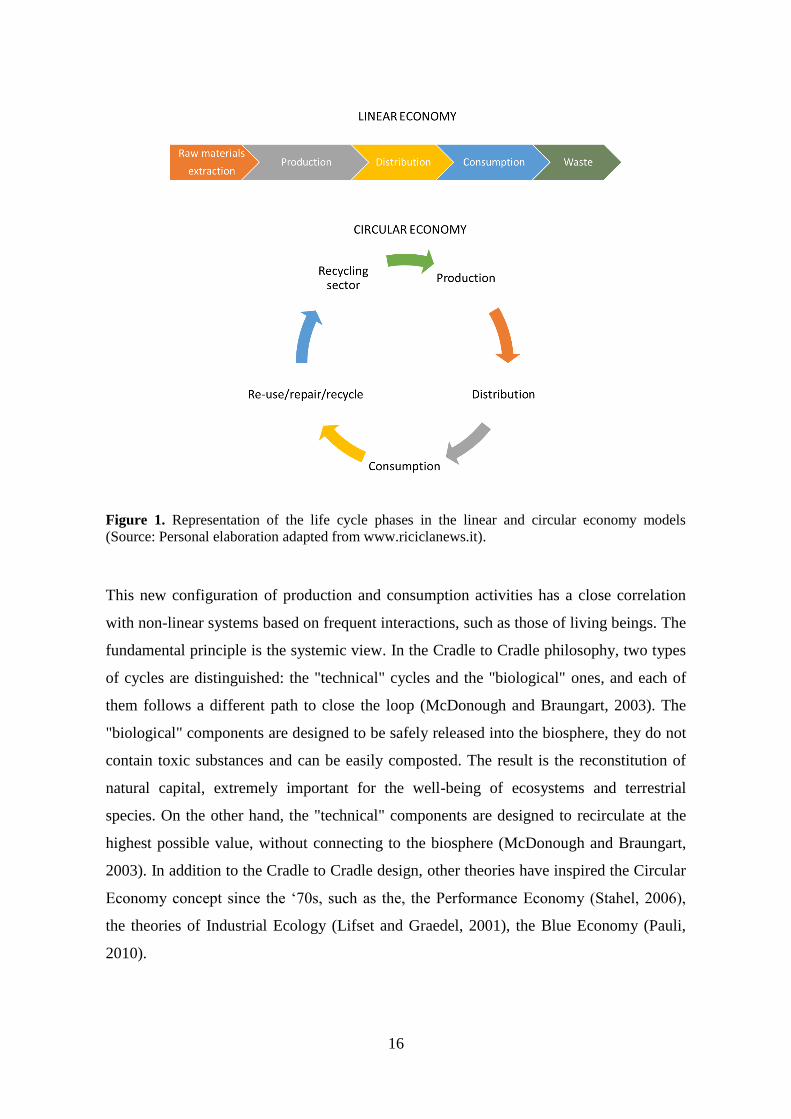
16
Figure 1. Representation of the life cycle phases in the linear and circular economy models
(Source: Personal elaboration adapted from www.riciclanews.it).
This new configuration of production and consumption activities has a close correlation
with non-linear systems based on frequent interactions, such as those of living beings. The
fundamental principle is the systemic view. In the Cradle to Cradle philosophy, two types
of cycles are distinguished: the "technical" cycles and the "biological" ones, and each of
them follows a different path to close the loop (McDonough and Braungart, 2003). The
"biological" components are designed to be safely released into the biosphere, they do not
contain toxic substances and can be easily composted. The result is the reconstitution of
natural capital, extremely important for the well-being of ecosystems and terrestrial
species. On the other hand, the "technical" components are designed to recirculate at the
highest possible value, without connecting to the biosphere (McDonough and Braungart,
2003). In addition to the Cradle to Cradle design, other theories have inspired the Circular
Economy concept since the ‘70s, such as the, the Performance Economy (Stahel, 2006),
the theories of Industrial Ecology (Lifset and Graedel, 2001), the Blue Economy (Pauli,
2010).
Page 25
17
The circular economy model is established on three main principles (Ellen MacArthur
Foundation et al., 2015):
The protection and growth of natural capital, through the control of limited
quantities of non-renewable resources and the balancing of flows of renewable
resources.
The optimization of the resource productivity by means of the permanence in the
"biological" or "technical" cycles of products, components and materials, at the
highest possible value.
The centrality of the identification of environmental impacts and a design that
excludes negative externalities, in order to achieve system effectiveness.
The transition to the circular economy model can lead to several opportunities and benefits
from the economic, environmental and social point of views (Ellen MacArthur Foundation
et al., 2015). As regards the economic advantages, they would be the revenue increase
from circular economy activities and the decrease of production costs due to the increase
in the utilisation rate of resources as well as the employment growth and greater
innovation, by means of new technologies and higher production efficiency. Several
benefits for the environment would also occur, such as the reduction of carbon dioxide
emissions into the atmosphere, the lower consumption of virgin materials, the reduction of
both land use and the release of toxic substances. Finally, circular economy will also
benefit the society and consumers, because there would be increased spending
opportunities, due to products and services lower prices, customisation of products
according to people needs and reduced products obsolescence (Ellen MacArthur
Foundation et al., 2015).
2.1 European policies for circular economy
In the framework of sustainable development policies, the European Commission has
developed in 2011 a Roadmap to Resource Efficient Europe (COM (2011) 571) (European
Commission, 2011), which is part of the Europe 2020 strategy (COM (2010) 2020)
(European Commission, 2010) for a competitive, inclusive and sustainable European
economy. It aims at both increasing the productivity of resources and reducing the
environmental impacts for the decoupling of economic growth from the environmental
burdens. The Roadmap foresees several actions in this context, such as the development of
Page 26
18
new sustainable production and consumption models, with the focus on the entire products
life cycles, the reduction of waste and losses by 50%, with particular attention to the agri-
food sector, the valorisation of waste, by means of recovery, recycling and regeneration;
the financing of eco-innovation projects; the elimination of environmentally harmful
subsidies, the protection of natural ecosystems and biodiversity; the reduction of land use
and improvement of soil quality; the identification of improvement solutions for those
sectors with a considerable environmental impact, i.e. food, construction and mobility.
Therefore, the Roadmap includes several main topics related to circular production and
consumption systems and the development of the circular economy within the European
market, in order to obtain a greater global competitiveness, to support the sustainable
growth and the employment growth.
A further action plan, "Closing the loop – An EU Action Plan for Circular Economy"
(COM (2015) 614) (European Commission, 2015) involves all phases of the products life
cycle. According to EU, “Circular economy systems keep the added value in products for
as long as possible and eliminates waste. They keep resources within the economy when a
product has reached the end of its life, so that they can be productively used again and
again and hence create further value” (European Commission, 2014b). The solutions
proposed by the Action Plan include eco-design, the choice of sustainable production
techniques, the creation of industrial symbiosis projects and the adoption of the Extended
Producer Responsibility policies. The consumption phase is supported by the introduction
of environmental and energy labelling for products, the use of eco-design to extend the
product’s life, by its reuse and repair, with the aim to avoid waste production, the
reduction of household waste, the promotion of Green Public Procurement, the
development and favouring of sharing economy models to share products and
infrastructures and to boost the consumption of services rather than of products. The waste
management actions include the compliance with the waste hierarchy, established by the
EU in 2008 (prevention, preparation for re-use, recycling, energy recovery, disposal),
prioritizing the waste reduction by eco-design and the recovery of the highest possible
value, also increasing the recycling rate.
Furthermore, the Action Plan highlights that a market for recycled materials and
secondary raw materials will be promoted, including recycled nutrients, with the aim to
reduce the extraction of virgin materials. New sources of investment to finance innovative
projects in the circular economy field will be introduced as well. Finally, circular actions
Page 27
19
will be developed for some priority sectors, such as: 1) plastics, to increase their recycling
and biodegradability and the recycling of plastic packaging; 2) food waste, to develop a
common methodology for quantifying them as well as measures to facilitate the food
donation and the use of by-products for feed production; 3) critical raw materials, to
encourage their recovery; 4) construction and demolition waste; 5) biomass and biological
products to promote the efficient use of bioresources and to support innovation in the
bioeconomy field (European Commission, 2015).
Page 28
20
3 Circular economy in the agri-food sector
3.1 Problems of the linear economic model in the agri-food sector
The agri-food sector involves 40% of the European land, contributes to satisfy one of the
most important human needs, i.e. nutrition, provides several ecosystem services essential
for our planet as well as social and cultural and economic value (European Environmental
Agency, 2015; Notarnicola et al., 2017). Nevertheless, several risks threaten the stability
of the linear economic model and the agri-food sector will suffer significant direct
consequences, if appropriate offsetting measures will not be established. The Department
of Agriculture of the U.S.A and Food and Agriculture Organisation (FAO) estimate that
by 2030 there will be a greater demand for crops, equal to 40-50% higher than that of
2010 (Ellen MacArthur Foundation, 2013b). Moreover, the doubling of agricultural food
production during the past 35 years was associated with a significant increase (from 1.1 to
6.87-fold) in nitrogen and phosphorus fertilization, in the amount of irrigated cropland and
in land for cultivation (Fantin et al., 2017; Tilman et al., 2002). Intensive agricultural
production has thus had strong impacts on the diversity, composition, and functioning of
the natural world ecosystems and on their capacity to provide society with a variety of
ecosystem services (Fantin et al., 2017; Tilman, 1999).
The combined use of mineral fertilizers, pesticides and massive irrigation, generated great
prosperity in agriculture, satisfying the growing demand for products. Nevertheless, the
trend has been reversed in the last years: the land productivity has been reduced and it was
not able to satisfy the demand of the growing world population. In the next few years,
hectares of fertile land will decrease by 25-35% compared to the 1.5 billion currently
cultivated (Ellen MacArthur Foundation, 2013b). In addition, due to an increasingly
intensive and industrialized agriculture, another important form of degradation is soil
nutrient depletion. The high use of mineral fertilizers has caused negative imbalances in
the soil characteristics, causing an excess of nutrients withdrawn from the soil compared
to input nutrients, eutrophication phenomena, the destruction of biodiversity and the
increase in the concentration of greenhouse gases in the atmosphere, due to increasingly
specialized agricultural techniques based on fossil fuels consumption (Ellen MacArthur
Foundation, 2013b). As regards direct environmental impacts, the food and drink
production chain in the EU causes 17% of the greenhouse gases direct emissions and 28%
Page 29
21
of the natural resource use and the consumption of meat requires involves a huge
utilisation of water (European Commission, 2011).
A further critical issue in the agri-food sector is the loss of value throughout the supply
chain, e.g. crops damage due to climatic and environmental conditions, losses of
agricultural products which do not comply with market standards and the degradation
during transport and storage (Ellen MacArthur Foundation et al., 2015). The use of water
for agricultural purposes is a quarter of the total water demand, and almost 25% is lost
during the transfer to the final point (European Environmental Agency, 2012). In the
processing phases, 8% -12% of inputs are lost, without contributing to the final value,
frequently due to non-optimised processing techniques or to strict specifications for
finished products (FAO, 2011). The problem of the lost value in the distribution phase
concerns mainly developing countries, where, in the post-harvest phases, the conservation
and the sale of agricultural products are not efficiently managed. In developed countries,
this loss occurs mainly in the use phase, where a large quantity of food is purchased but
not consumed (FAO, 2011). It is estimated that around 30% of the food produced is
wasted (FAO, 2011). In particular, 90 million t of food are wasted every year in Europe,
equal to 180 kg per person (European Commission, 2011). Finally, a great loss of value
occurs in the post-consumption phase, where large quantities of food waste are not further
recovered and are treated as waste (FAO, 2011). The agricultural sector is therefore a
major contributor to the waste stream stemming from the linear production and
consumption model. Because of these reasons, the lack of environmental sustainability can
negatively affect the functioning of the agri-food supply chain, in terms of production of
safe food with a fair cost, and more in general the competitiveness of the agri-food
industry (European Commission, 2014a).
Therefore, a transition towards circular economy models in the agri-food supply chain,
which include sustainable production and consumption patterns, is required, which would
increase system productivity while decreasing its environmental impacts (European
Commission, 2014a). Without this systemic shift, the environmental impacts of the agri-
food supply chain will increase significantly in the next years and probably they will
exceed the planetary boundaries (Notarnicola et al., 2017).
The circular economy model aims to overcome the limits of the current system, moving
from maximizing the performance of individual elements to optimizing the entire agro-
Page 30
22
food system: the increase in performance must be followed by the improvement of quality
of soil, water and air (Ellen MacArthur Foundation et al., 2015).
The application of circular economy concept in the agri-food production chain involves
the reduction of waste, the utilisation of by-products and food waste, the recycling of
nutrients (Jurgilevich et al., 2017), the sustainable use of resources (soil, land, water,
biodiversity), the use of renewable natural resources (i.e. biomass), the avoidance of food
waste and surplus (Rood et al., 2017), the production and consumption of products with a
better environmental performance throughout their life cycle, the application of both
cleaner technologies and eco-innovation in production processes. In these ways, the
resources will be used efficiently within a life cycle of a product, and waste produced will
be both minimized and re-used as much as possible in other production chains, thereby
providing economy with added value and causing lower environmental impacts
(Rigamonti et al., 2017). All the above measures must be implemented both at the
producer and consumer levels and in the waste management systems (Jurgilevich et al.,
2017).
3.2 Benefits of the circular economy in the agri-food sector
The benefits of maintaining the components of agro-food products within "biological"
cycles can be summarized in three macro-categories: the supply of new raw materials,
such as the bio-chemical substances contained in waste, soil regeneration and energy
production (Ellen MacArthur Foundation et al., 2015). The extraction of components with
excellent chemical-physical properties takes place within bio-refineries, which process
organic materials, such as agricultural residues and food waste, to obtain chemical and
biofuel substances. The food industry can capture all the value contained in waste and by-
products by exploiting the cascade use. The involvement of all stakeholders, such as
industry associations and government bodies, as well as companies, is essential for
creating favourable conditions for new business ideas (Ellen MacArthur Foundation et al.,
2015). A major role to obtain these objectives is played by technological and process
innovation. A main feature of the circular economy in the agri-food sector is the capacity
of soil restoration in order to promote a higher fertility rate, thus increasing crop
productivity. Manure and other food and animal waste can be used for this purpose, in
order to avoid the massive use of chemical fertilisers. Finally, energy can be obtained
Page 31
23
from food waste through anaerobic digestion (which produces also digestate with good
fertilising properties) and waste incineration (Ellen MacArthur Foundation et al., 2015).
Several advantages can stem from the redesign of the agri-food sector in a circular
economy approach. The annual expenditure of food products per family would be reduced
by 25% by 2030 and by 40% by 2050, thanks to the decrease in food waste (Ellen
MacArthur Foundation et al., 2015). From the environmental point of view, there would
be significant reductions in the use of pesticides, chemical fertilizers, energy, soil, water
and in the emissions of greenhouse gases. There would be also a job growth due to the
increase in the organic farming practices and to waste management systems. In economic
terms, the implementation of the circular model would bring an economic benefit of € 320
billion compared to the current system, due to the reduction of costs for primary resources
procurement and the decrease in externality costs (Ellen MacArthur Foundation et al.,
2015). It is important to highlight that, in the transition to a new agri-food system, the
introduction of innovative technologies and systems aimed at reducing waste should be
coupled with policy actions to promote the resource efficiency goals, the restoration of
natural capital and the production of high-quality products (Ellen MacArthur Foundation
et al., 2015). Moreover, the transition to circular economy in the agri-food production
chain requires joint efforts of farmers, food companies, retailers and consumers and the
use of resource efficient production techniques (e.g. precision agriculture practices,
organic agriculture and digitalisation of supply chains) as well as sustainable food choices
and a decrease in food waste (European Commission, 2011; Ellen MacArthur Foundation
et al., 2015).
Page 32
24
4 Life Cycle based methods to support the transition towards
circular economy in the agri-food sector
The transition towards sustainable consumption and production systems in the agri-food
sector, in a circular economy approach, requires the use of robust and scientific methods
and tools which can support sustainability assessment of the overall analysed system for
several sustainability indicators, by appropriately evaluating the consequences of all the
possible circular options, both from an economic, environmental and social point of view.
For the assessment of the circular economy impacts, the application of the Life Cycle
Thinking (LCT) approach, which takes into account the whole life cycle, can be an
adequate solution with many benefits.
At international level, it is recognized that sustainability assessment must be based on a
LCT approach, which aims to identify improvement opportunities for all phases of
products life cycles, in terms of reduced environmental impacts and greater resource
efficiency, thus avoiding burden shifting from a phase to another of the life cycle, and
from an environmental compartment to another (Fantin, 2012). This holistic vision of the
production system allows to consider the contribution of each process which fulfils the
function for which it was designed. Cooperation along the value chain is essential to reach
these goals, for sharing all the information and knowledge required for a complete and
detailed study.
Par. 4.1 and 4.2 of this chapter are partially based on the following publications,
performed during the PhD:
Chiavetta C., Fantin V., Cascone C., 2017. L’Economia Circolare nel settore
agroalimentare e il Life Cycle Assessement come strumento a supporto: il
progetto FOOD CROSSING DISTRICT. ENEA Technical report, USER-PG64-
003, June 2017 (Confidential).
Ferrara M. Fantin V., Righi S., Chiavetta C., Buttol P., Bonoli A., 2017.
Applicazione della Water Footprint sviluppata dal WF Network: il caso del
Pomodorino del Piennolo del Vesuvio DOP. In Proceedings of XI Conference of
Italian LCA Network Association, Siena, 22-23 June 2017, ISBN 978-88-8286-
352-4.
Page 33
25
4.1 Life Cycle Assessment
From the environmental point of view, Life Cycle Assessment (LCA) is an internationally
accepted and standardised method (ISO 2006 a, b) which is recognized as a strategic and
effective tool to evaluate the potential environmental impacts occurring in the whole
product's life cycle as well as to identify possible areas for improvement (Fantin et al.,
2014). Because of these reasons, LCA method could support the analysis of the impacts
and benefits associated to circular solutions, also by a preventive approach, thus
contributing to increase the sustainability of current sustainable production and
consumption models (Sala et al., 2017). Since the LCA analysis considers the entire agri-
food value chain, both the identification of food systems environmental impacts and the
consequent improvement solutions aim to increase the resource and energy efficiency of
the supply chain while decreasing their environmental burdens (Notarnicola et al., 2017).
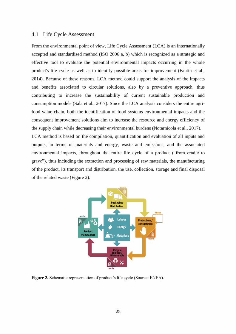
LCA method is based on the compilation, quantification and evaluation of all inputs and
outputs, in terms of materials and energy, waste and emissions, and the associated
environmental impacts, throughout the entire life cycle of a product (“from cradle to
grave”), thus including the extraction and processing of raw materials, the manufacturing
of the product, its transport and distribution, the use, collection, storage and final disposal
of the related waste (Figure 2).
Figure 2. Schematic representation of product’s life cycle (Source: ENEA).
Page 34
26
LCT approach has been adopted by the European Union within the Integrated Product
Policy (IPP) (European Commission, 2003) and in Sustainable production and
consumption policy (European Commission, 2008) which propose the application of
several actions to promote the continuous improvement of products environmental
performance throughout their entire life cycle. LCA method and LCT approach are used
also in environmental communication. In fact, they are the basis of both ISO 14020
compliant ecological labels, such as the European Ecolabel, and the Environmental
Product Declaration (EPD) and Green Public Procurement. LCA can therefore support
companies in the identification of opportunities for the improvement of the environmental
performance of products, in the selection of key environmental indicators for monitoring
their environmental performance, in marketing processes, e.g. to obtain ecological product
labels and in the eco-design of product and processes.
The first examples of LCA method were in the 1960s and 1970s in the USA but the
interest in its application grew in the 1990s. In 1993 the Society of Environmental
Toxicology and Chemistry (SETAC) defined as LCA as an objective assessment of energy
and environmental impacts related to a product, process or activity, carried out by means
of the identification of energy and materials consumption and waste released into the
environment (SETAC, 1993). The evaluation includes the entire life cycle of the product,
process or activity, including the extraction and processing of raw materials,
manufacturing, transportation, distribution, use, reuse, recycling and final disposal
(SETAC, 1993). In 1998 SETAC created a series of guidelines that were then included in
the ISO 14040 standard. According to ISO 14040 standards (ISO, 2006a, b), it consists in
the “compilation and evaluation of the inputs, outputs and the potential environmental
impacts of a product system throughout its life cycle” (ISO, 2006a) and involves four
main phases: the goal and scope definition, the Life Cycle Inventory analysis (LCI), the
Life Cycle Impact Assessment (LCIA); and the Interpretation of results (Figure 3).
Page 35
27
Figure 3. Four main phases of LCA method (Source: Personal elaboration adapted from ISO,
2006a).
LCA method shares with the circular economy the perspective connected to the
consideration of the life cycle as a whole. LCA can thus support effectively the
implementation of circular economy principles, because it allows to choose the solution
with the lowest environmental impacts. More in detail, the application of this method can
contribute to verify the hypotheses formulated in the business planning phase, highlighting
for example any negative consequences due to a particular configuration. In addition,
LCA can help to identify improvement opportunities by the evaluation of the possible
alternatives and limits of the current scheme and then it could provide new ideas for the
design phase. Finally, it can support the formulation of new objectives at a strategic level,
by means of the creation and monitoring of specific performance indicators to encourage
continuous environmental improvement (Chiavetta et al., 2017).
Circular economy offers a vision which can influence the way companies and
governments operate. The support of a scientific method such as LCA can guarantee that
this vision is translated into concrete benefits for people and for the natural capital.
Ultimately, LCA provides substantial quantitative measures on which choices at product
level are based, thus demonstrating its potential as a complementary tool for the circular
economy (Chiavetta et al., 2017).
Page 36
28
4.2 Water Footprint
Another life-cycle based tool developed in the last years and progressively used in the
agri-food sector, also for communication purposes, is Water Footprint (WF), which is an
assessment of the water use by products, individuals, companies or the entire population.
Water is indeed a natural resource essential to support human life and activities, although
the problem of water scarcity is recognized as one of the major environmental issues at
world level (Manzardo et al., 2016). According to a recent FAO report (FAO & WWC,
2015), in the next decades agriculture will continue to be the major contributor to water
use and water pollution, contributing on average for more than half of water withdrawals
from rivers, lakes and aquifers. In fact, the quantity of global water used for irrigation
purposes is estimated to increase from 2,600 km3 in 2007 to 2,900 km
3 in 2050, with a
great increase especially in developing countries (FAO &WWC, 2015). Moreover, the
increasing water demands in urban areas and businesses will decrease the volume of water
available for agricultural production (FAO &WWC, 2015).
In Europe, one third of the water consumption is utilised in the agricultural sector, which
influences both the quantity and quality (i.e. pollution from pesticides and fertilizers) of
water available for other applications (EEA, 2012). In the southern European countries,
such as Italy, Greece and Spain, about 80% of water used in agriculture is for irrigation
purposes, due to the semi-arid climate conditions (EEA, 2012). Italy is one of the
European countries that mostly use irrigation (ISTAT, 2014). The volume of irrigation
water used in Italy in 2009-2010 was 11,618 milion of m3. Most of the water use takes
place in agricultural systems located in North-Western Italy (6,800 m3/ha) and in North-
Eastern Italy (2,500 m3/ha), followed by Central and Southern regions (3,500 m
3/ha).
The problems of water scarcity and pollution occur locally, but the protection and efficient
management of water resources must be pursued at national and transnational level, as
implemented by the “Blueprint to safeguard Europe's water resources” (COM,
2012/0673). In this context, it is therefore essential to have tools and methods to
understand how we are influencing the use of this resource with our production and
consumption choices as well as to evaluate the results of companies and governments
policies for sustainable water use (Ferrara et al., 2017).
Page 37
29
In the last years, the WF concept has emerged, which is an assessment of the water use
that has created a lively discussion within the scientific community (Pfister et al., 2017),
because two methods, both based on a LCT approach, have been developed in parallel:
1) The Water Footprint Network (WFN) (www.waterfootprint.org) developed and
published in 2011 the Water Footprint Assessment Manual (Hoekstra et al., 2011),
which underlines the necessity to involve consumers and producers in the water
management along the production chain;
2) The LCA community has developed methods to include the environmental impacts of
water use throughout the product’s life cycle in LCA studies and has contributed to
the definition of the underlying concepts of the ISO 14046 standard (ISO, 2016).
The product WF developed by the WFN is defined as the volume of freshwater used
throughout the production process. This indicator provides a measure of the amount of
water available which is used by humans, dividing water into three components: blue,
green and grey. The blue component refers to the consumption of water taken from a
surface water body or groundwater; the green component expresses the consumption of
rainwater that, once have reached the soil, does not flow or recharge the groundwater, but
is used in the evapotranspiration process of the soil-plant system; the grey component is
the volume of fresh water required to bring the concentration of a given load of pollutants
below the maximum values established by legislation (Hoekstra et al., 2011).
The WF according to ISO 14046 is based on the LCA method (ISO 14044) and is defined
as a measure that quantifies all the potential environmental impacts related to water used
or influenced by a product, process or organization. According to ISO 14046, a WF
evaluation means that all the potential impacts related to the use of water are taken into
account, otherwise the indicator to which it refers must be specified (e.g. ”water scarcity
footprint” or “water eutrophication footprint”). In the framework of the Life Cycle
Initiative, the UNEP/SETAC WULCA (Working Group on Water Use in LCA) has dealt
with the problem of harmonizing and achieving consensus around an impact assessment
method for freshwater consumption. Currently, it has developed the midpoint indicator
AWARE (Available WAter REmaining for area in a watershed), which represents the
water available per unit of surface which remains in a basin after having satisfied the
demand from humans and ecosystems (UNEP / SETAC, 2016). Characterization factors
for this method have been developed per year and country, for agricultural and non-
agricultural uses. This indicator only evaluates the blue water scarcity and it does not
Page 38
30
consider rainwater (i.e. green water) (Boulay et al., 2013). Both methods have been
applied to the agri-food production chain in the past 10 years (Zhang et al., 2017) and can
be useful to support a sustainable management of water resources (Boulay et al., 2013) as
well as the development and implementation of green marketing strategies addressed to
both companies and consumers (Symeonidou & Vagiona, 2018). Moreover, some recent
studies combine the use of WF Network method and ISO 14046 to compare the
consistency of the obtained results and to evaluate both their strengths and weaknesses
(Manzardo et al., 2016; Bai et al., 2018).
4.3 Application of LCA in the agri-food sector: main methodological
problems
LCA method has been increasingly applied to the agri-food sector for the evaluation of the
environmental impacts of a wide variety of agri-food products, contributing to both
identify the environmental hotspots of the supply chain and the improvement
opportunities, thus supporting political and institutional decisions (Notarnicola et al.,
2012). Nevertheless, when applying LCA to food and drink products, the practitioner has
to deal with methodological problems which stem from the peculiarities and specific
characteristics of the agri-food supply chain. In fact, differently from industrial production
systems, these systems have complex relationships, which are difficult to be modelled in
LCA studies, between inputs (for example nutrients and soil) and outputs (crops and
emissions), between cultivation techniques and the maintenance of long-term soil quality
and in general terms between biological and technological processes (Fantin, 2012).
However, when LCA is used to communicate the environmental performance of agri-food
products, the different scientific approaches used to deal with the methodological issues
might lead to different LCA results, making it difficult to compare the environmental
performance of products of the same category. The European Commission’ Product
Environmental Footprint (PEF) recommendation, developed in 2013 (European
Commission, 2013a), and the integrating documents aim to fulfil the need for
harmonisation to calculate and communicate environmental footprint of products.
In particular, some critical issues on which different scientific approaches have been
applied are the definition of the functional unit, the system boundaries and the allocation
procedures, the calculation of on-field emissions from the use of fertilizers and pesticides
at inventory level, the comprehensive assessment of toxicity impacts from the use of
Page 39
31
pesticides and the definition of some impact categories indicators, such as water use or
land use (Notarnicola et al., 2012). Moreover, LCA method does not take into account in a
comprehensive way some specific features of agri-food production chains, which are
important to maintain the sustainability of food production, such as the decrease in soil
quality, including the long-term effects of agricultural practices on the soil fertility, the
increase in soil erosion, the reduction of ecosystem services, the loss of biodiversity and
the nutritional and organoleptic properties of food products, which are difficulty to be
quantified (Fantin, 2012). It is also important to point out that the analysis of some of the
above aspects should require information at the landscape level, which is not accounted
for in LCA method (Notarnicola et al., 2017).
Besides, other main challenges in LCAs of food systems are the the assessment of land
use change, the lack of spatial and temporal characterisation in food LCA databases and
life cycle impact assessment models and the exclusion of cultural values, which can affect
the food production and consumption as well as the evaluation of the environmental
impacts of agri-food supply chains (Hauschild et al., 2012; Notarnicola et al., 2017).
In the following paragraphs, some of the main critical methodological issues of the
application of LCA method to agri-food supply chain will be analysed.
4.3.1 Definition of the functional unit
The functional unit is defined by ISO 14040 as the quantified performance of a product
system, to be used as a reference unit. Therefore, it provides the reference to which inputs
and outputs of the studied system will be connected and it is necessary to ensure the
results comparability among different products with the same function. The functional unit
is thus a crucial point in defining the scope of the LCA study, and is connected to the goal
of the study, to the function of the product and to the analysed system.
It is important to highlight that the choice of different functional units for the same
product system can affect the results of the study (Notarnicola et al., 2012).
According to Reap et al. (2008), the definition of the functional unit is one of the major
methodological problems in the goal and scope definition of the LCA method. The authors
explain that several sources of errors can occur when functional unit is chosen. For
example, an inaccurate definition of the functions of the system can lead to a wrong
representation of the reality. Moreover, products often have multiple functions, which
should be considered to properly reflect reality, or their function could be not easily
Page 40
32
quantified. In this context, a further problem arises, i.e. how to choose the most proper
functional unit which represents more functions (Cooper, 2003; Reap et al., 2008).
In LCA studies of agri-food systems, the main function of the system is considered to be
human nutrition (Nemecek et al., 2016) and does not include multiple function that the
product may have, such as the energy or nutrient content or the provision of a pleasant
texture or taste (Reap et al., 2008, Shau and Fet, 2008). Therefore, the functional unit is
frequently based on the mass or volume of the product (Roy et al., 2009, Schau and Fet,
2008; Kendall and Brodt, 2014; Roma et al., 2015; Petti et al., 2015). However, alternative
functional unit may also be chosen, for example the nutritional or economic values of the
product and land area.
The choice of mass or volume for the identification of the functional unit can be seen as a
simplified approach, because the agricultural system is supposed to have one only
function, i.e. the production of the main product. Moreover, this kind of functional unit
can support the comparability between LCA studies of products of the same product
category, but it does not consider the benefits derived from these products, especially their
nutritional values (Heller et al., 2013). Moreover, the use of a physical amount of output
as functional unit for food products can be misleading for consumers, because sometimes
an inverse correlation exists between the yield and product’s quality. In fact, several
authors found that organic products, which are perceived by consumers as added value
products from both environmental and health point of views, and local typical productions
can have higher impacts per unit of product, due to lower production yield (Tuomisto et
al., 2012). Similarly, many LCA studies highlight that intensive agriculture practices leads
to lower environmental impacts per functional unit, when it is defined as mass or volume,
because they have higher yields, which split the environmental impacts of the product to a
larger amount of output (Notarnicola et al., 2017; Sonesson et al., 2016; Kulak et al.,
2013; Kiefer et al., 2015).
Other possible functional units found in literature are the cultivated area (Shau and Fet,
2008; Petti et al., 2015), the energy or protein content (Shau and Fet, 2008; Renzulli et al.,
2015), the content of glucose and fructose (Renouf et al., 2008), the serving size (Roma et
al., 2015), the dry biomass production (Renzulli et al., 2015) and the economic value
Notarnicola et al., 2017), although different types of external factors, which are not always
connected to product’s quality, can affect products’ prices (Notarnicola et al., 2017).
Page 41
33
Due to the different functions of the food product systems, it could be useful to adopt
multiple functional units in order to evaluate the variability of LCA results and to increase
its robustness, thus analysing the product system from different perspectives (Notarnicola
et al., 2012). Therefore, several authors used multiple functional units in the same study,
such as the mass of products, the energy or protein content, the cultivated area, the unit of
livestock and the economic value (Sala et al., 2017). For example, Salou et al. (2016) used
two functional units for the assessment of environmental performance of dairy systems: t
of milk and area of land occupied and demonstrated that different functional units lead to
completely different results (Sala et al., 2017). The same results were obtained by Kendall
and Brodt (2014) and Van Kernebeek et al. (2014) (Nemecek et al., 2016). Similar results
were obtained also by Cerutti et al. (2014), which compared the same fruit production
chains with different functional units. More in detail, fruit cultivars with higher yields
have lower environmental impacts when using mass as a functional unit, whereas fruit
cultivars with lower yields show a better environmental performance when land areas is
used as functional unit.
A further aspect that should be taken into account in the definition of the functional unit of
agri-food products is the quality of the product, expressed not only as nutritional content,
but also as taste, texture, cultural, social and ethical values, which can be connected to the
territory and landscape protection. Nevertheless, since it is not possible to include all these
issues in a single functional unit, the practitioner must unambiguously declare the chosen
function and analyse also the consequences of their choice (Nemecek et al., 2016). For
example, 1 L of virgin olive oil cannot be compared with 1 L of olive oil, because these
products are different from the qualitative point of view (Salomone et al., 2015).
Consequently, it should be highlighted that the definition of the most correct functional
unit is rather difficult when product quality is included in the system function (Notarnicola
et al., 2012).
A further important feature for the identification of the most suitable functional unit for
food products is the problem of food waste. In fact, wasted food increases the
environmental burdens of the consumed food, because a higher quantity of product is
required to satisfy the product’s function (Cerutti et. al., 2014; Nemecek et al., 2016).
Therefore, the quantification of food losses throughout the supply chain should be
included in the assessment in order to evaluate the actual environmental performance of
the product consumed (Cerutti et al., 2014; Ingwersen, 2010), although the quantification
Page 42
34
of food waste in the different stages of the life cycle is often difficult and is also affected
by consumers practices (Nemecek et al, 2016). In some literature studies on fruit and
vegetables production, the environmental impacts of discarded products were attributed to
the functional unit, which was defined as the net yield or the marketable yield (Mogensen
et al., 2015; Romero-Gámez et al., 2014; Corrado et al., 2017). Manfredi M. et al. (2015)
defined the functional unit as the delivery of eaten food, as suggested by Wikstrom et al.,
(2014).
Finally, it is important to point out that the choice of the functional unit based on mass,
volume or nutrient content seems to be more adequate for the communication to
consumers, in order to direct them towards consumption models with a better
environmental performance (Nemecek et al., 2016; Finkbeiner, 2014). Moreover, at the
moment, this approach is methodologically the most robust and investigated and it is
adopted by the European Commission’s Product Environmental Footprint (PEF) method
(European Commission, 2013a) within the Single Market for Green Products Initiative
(European Commission, 2013b) for the assessment of the environmental performance of
agri-food products.
4.3.2 System boundaries definition
According to ISO 14040-44, the selection of the system boundaries establishes the unit
processes, activities and operations to be included in the LCA study. The choice of the
processes to be included or excluded depend on the goal and scope of the study and both
the data quality and availability (Salomone et al., 2015). System boundaries should
include all the relevant life cycle stages and processes of the studied production chain. In
fact, the environmental assessment of food products should at least consider the supply
chain up to the point of sale, including agricultural production, processing, by-product
management, transportation, distribution, although the whole supply chain, thus including
also the transport up to the consumer, the food chilling and cooking and the waste
management should be taken into account for a more comprehensive evaluation of
environmental performance. (Nemecek et al, 2016; Salomone et al., 2105).
Nevertheless, in literature LCA studies of agri-food products, the lack of data on some
specific processes frequently lead to their exclusion from the system boundaries, and the
goal and scope of the study have to be re-delineated accordingly (Salomone et al., 2015).
However, it is important to highlight that ISO 14044 permits the exclusion of life cycle
Page 43
35
stages and processes only if they do not change the results of the study, and that any
decision must be clearly stated and the reasons and implications for their emissions must
be explained (ISO, 2006). Moreover, an inappropriate selection of system boundaries or
the exclusion of some unit processes can affect final results, thereby leading to incorrect
considerations and decisions, also from the decision maker point of view (Reap et al.,
2008). In particular, this problem affects the comparison between different studies, which
can be rather difficult (Graedel 1998; Lee et al., 1995; Reap et al., 2008; Shau and Fet,
2008).
In literature agri-food LCA studies, the most used system boundaries are the following:
1) “from cradle to farm gate”, including only the cultivation phase (for fruits and
vegetables supply chains) or the cultivation and animals breeding phases (for
livestock supply chains) (Roma et al., 2015; Cerutti et al., 2015; Renzulli et al., 2015;
Castanheira et al., 2010; Guerci et al., 2013a, b; Zhang et al., 2013; Khoshenivesan et
al; 2013;
2) “from cradle to processing factory gate”, which include both agricultural processes
and transformation and processing phases (Roma et al., 2015; Cerutti et al., 2015;
Renzulli et al., 2015; Fantin et al., 2017; Gonzales-Garcia et al., 2013a; Opio et al,
2013).
Most studies therefore do not consider the consumption, use and end-of life of the product
(Petti et al., 2015), which however have a major importance due to the great quantity of
food which is wasted at households every year, equal to 46% of the total amount of wasted
food at European level in 2006 (European Commission, 2014a), considering also that one
third of the edible parts of food is wasted (FAO, 2011). In this context, LCA studies of
food products could have an important role because they could contribute to evaluate the
potential savings of avoiding food waste, although food waste is still frequently assessed
incompletely in literature (Corrado al, 2017). In addition, both the consumer transport and
food preparation can have remarkable impacts (Nemecek et al., 2016) and should be
included.
4.3.3 Allocation procedures
Allocation means “partitioning the input and output flows of a process or a product system
between the product system under study and one or more other product systems” (ISO,
2006a) and must be carried out when the system under examination produces two or more
Page 44
36
products, such in the case of many agri-food systems (for example milk and meat
production).
This means that allocation can divide the total environmental impacts of the multi-
functional process among each function or product. As already explained for the definition
of system boundaries, inaccurate allocation can affect LCA results and lead to incorrect
decisions (Reap et al., 2008). ISO 14044 suggests to use the following procedure for
processes which have more than one outputs:
1. Avoid allocation by (1) separating multifunctional processes into sub-processes and
collecting the data for each process and/or (2) expanding the system boundaries to
include the additional functions of the co-products;
2. If allocation cannot be avoided, it should be performed according the underlying
physical relationships between the different products or functions of the system;
3. If allocation based on physical relationships is not viable, the environmental
burdens of each product should be allocated on the basis of other relationships (e.g.
the economic value of products).
However, each of the above steps can have some limitations and difficulties (Reap et al.,
2009). The subdivision of multi-functional processes involves the collection of more
detailed information about the processes and should be performed when this information
can be collected at an affordable cost, or when the processes are independent from the
economic point of view (Shau and Fet, 2008; Ekvall and Finnveden, 2001). As regards
system expansion, there are mainly two approaches for performing it: 1) system
boundaries enlargement; 2) avoided burdens approach (Azapagic and Clift, 1999). This
means that the environmental impacts of alternative ways to produce the product or the
co-products are either added to the system or subtracted from it, with the aim to assure
their comparability. Nevertheless, both approaches require the identification of alternative
production systems suitable for substitution and the availability of inventory data for them
(Azapagic and Clift, 1999; Niederl-Schmidinger and Narodoslawsky, 2008). In addition,
system expansion leads to a more complex LCA model which requires more data to be
collected (with more temporal and economic efforts) and to potential uncertainty of data
quality (Curran, 2007; Reap et al., 2008; Notarnicola et al., 2017). Moreover, if the
practitioner applies system expansion without substituting the additional function of the
co-products, the functional unit will include more products. In this way, the product could
not be assigned easily to a certain product category. For example, in the application of
Page 45
37
system expansion without substitution to a milk and meat production system, the function
of the system would be the production of both milk and meat, which belongs to the
product category food but not to the product category milk or meat (Shau and Fet, 2008).
An example of system expansion with substitution in LCA studies of agri-food supply
chain is that performed by Cederberg and Stadig (2003) who compare the results obtained
with those coming from the application of economic allocation. In this study, the
combined milk and meat production system is expanded by including an alternative
production of meat, which is beef cows producing calves and meat. The environmental
impacts of the alternative meat production are then subtracted from the environmental
impacts of the combined milk and meat system, in order to obtain the environmental
burdens of milk production system. Results show that economic allocation between milk
and meat favours meat production, whereas when system expansion is applied, milk
production has a better environmental performance. This is due to milk co-products
(calves and meat from culled cows), because meat production in combination with milk
can be carried out with fewer animals than in meat production system. Therefore,
Cederberg and Stadig (2003) conclude that system expansion should be used to obtain
more robust results.
As regards the allocation based on physical relationship, it could be difficult to be
evaluated, because causality could be determined in several ways, or could not be easily
understandable (Finnveden et al., 2000; Reap et al, 2008). An example of physical
relationship in literature LCA studies of agri-food products is the biological causality
between the amount and type of feed intake and the outputs meat and milk (Cederberg and
Mattsson, 2000), the demand for feed needed for lactation, body maintenance and
delivering calves (Eide, 2002) or the mass of olive oil and the mass of pomace produced
by olive oil production process (Rajaeifar et al., 2014).
Finally, other relationships different from physical causality could be based on energy
content, mass, volume, economic value and they are frequently used in LCA studies
(Ekvall and Finnveden, 2001), mainly because they could be identified more easily and
data could be readily available (Reap et al, 2008). In general, economic allocation is the
most used approach in food LCA, because economic data can be easily obtained and the
economic value of the product is the motivation of the production process (Pelletier et al.,
2015; Notarnicola et al., 2017). In addition, agri-food products often have several by-
products with low economic value (e.g. fat and skin in cow slaughtering). The application
Page 46
38
of economic allocation to these by-products attributes them low environmental burdens
(Corrado et al., 2017). Furthermore, economic allocation can be applied in many different
contexts, because price reflects also the quality of products (e.g. cultural aspects, taste,
etc.) which cannot be measured by physical criteria and which drive consumers choices. In
addition, these particular characteristics connected to quality are unique and therefore
potential alternative processes cannot be identified, thus excluding the possibility to apply
system expansion or substitution (Ardente and Cellura, 2012).
On the other hand, economic allocation has some limitations, because prices are subject to
variability and sometimes prices and physical flows are not properly correlated. Both
issues lead to uncertainties and affect the reliability of LCA results (Ardente and Cellura,
2011; Marvuglia et al., 2010). In addition, ISO 14040 and International Reference Life
Cycle Data System (ILCD) Handbook (European Commission – JRC-IES, 2010) suggest
to use market prices of the co-products as the basis for economic allocation, although this
choice could be misleading, because prices should refer to the product’s value
immediately after its production and not to the final price at consumers, which could
reflect external factors (European Commission, 2011). According to Pelletier et el. (2015),
the LCA results obtained by economic allocation reflect market relationships (via price
ratios) rather than physical relationships. Problems can also occur when market prices are
not available. In those case, other sources can be used, such as historical prices and
expected prices (Guinée et al., 2004).
As regards food LCAs, several authors have applied economic allocation (Dalgaard et al.
2008; Blengini and Busto 2009; Gonzalez-Garcia 2013b; Beccali et al., 2010; Ayer et al.,
2007). For example, Beccali et al. (2010) highlight that in the production of fruit juices
and essential oils from citrus-based products, the essential oils are a small mass fraction of
company’s products, but they have a significant market price. In this case, substitution and
system expansion are not possible because alternative production processes for essential
oils cannot be identified; therefore the authors apply economic allocation because it
reproduces more correctly the causality of the production process. In the same way,
Gazulla et al. (2010) apply economic allocation to wine production because system
expansion is not viable in this case, since grapes residues and fermentation sediments
cannot be produced separately, and no detailed information is available about alternative
products which could be substituted by pomace and other by-products.
Page 47
39
In conclusion, allocation procedures and more in general the methods for solving the
multi-functionality of agri-food systems are still a topic of discussion at scientific level.
4.3.4 Emission models for pesticides and fertilisers emissions
Pesticides are applied intensively to agricultural fields in order to increase production
yields per unit of area and to control plant diseases. Nevertheless, these products can result
in severe environmental contaminations (Verna et al, 2014). Agricultural pesticide use is
substantial and amounts globally to about 1.2 million metric t of active ingredients (the
biologically active part of a commercial pesticide formulation) per year between 2005 and
2010 (FAO 2013). As reported by Verna et al. (2014), it has been verified that pesticides
applied to crops cultivation are degraded in several ways described as biotransformation,
biomineralization, bioaccumulation, biodegradation, bioremediation and cometabolism
(Shakoori et al., 2000; Park et al., 2003; Finley et al., 2010).
Pesticide biodegradation is a soil microbial function of critical importance for modern
agriculture and its environmental impact (Dechesne et al., 2014). A few biodegradation
controlling factors have tentatively been identified across pesticide classes. They include
some soil characteristics as pH (Rodriguez-Cruz et al., 2006; Bending et al., 2001, 2006;
El Sebai et al., 2007; Hussain et al., 2013; Rasmussen et al., 2005; Lauber et al., 2009;
Franco et al., 2009; Houot et al., 2000), soil moisture (Parkin and Shelton, 1992; Stenrød
et al., 2006; Rodriguez-Cruz et al., 2008; Monard et al., 2012; Hussain et al., 2013), C/N
ratio and potassium (Rasmussen et al., 2005), organic matter and clay (Rodriguez-Cruz et
al., 2006; Vinther et al., 2008). Other soil properties and characteristics partially related to
tillage practice such as macropores (Nielsen et al., 2010), structure and fractures (Alletto
et al., 2008) and soil horizons also have impact on pesticide degradation.
Pesticides and/or their degradation products are accumulated in diverse environmental
compartments such as plant, soil, air, surficial and deep groundwaters and lead to severe
environmental contaminations.
As explained above, LCA studies of agri-food systems have to face several main
challenges, such as the modelling of emissions from pesticides and fertilisers use at
inventory analysis level (Schmidt Rivera et al., 2017; Goglio et al., 2014), which can lead
to important environmental impacts to freshwater and marine ecosystems as well as to
terrestrial ones, due to their chemical, toxicological and eco-toxicological properties
(Notarnicola et al., 2017). The criticalities in modelling are due to several factors. Firstly,
Page 48
40
since data about their production are frequently not available, the practitioner often uses
estimates for the assessment, or excludes them from the study (Notarnicola et al., 2015;
Fantin et al., 2017; Schmidt Rivera et al., 2017). Secondly, even when the active
ingredients are considered, the pesticide and fertilizer formulation by-products (adjuvant,
solvents, etc.) are omitted from the analysis (Rosenbaum et al., 2015). Finally, the
calculation of on-field emissions due to the use of fertilisers and pesticides is rather
difficult and frequently they must be estimated by dispersion models, because their direct
measurement is not viable in LCA studies.
As regards the estimation of on-field emissions from pesticides at inventory level, the
main difficulty for the LCA practitioner is to quantify the amount emitted to the different
environmental media (i.e. air, soil, water), because the practitioner frequently knows only
the quantity applied to the agricultural field (Rosenbaum et al., 2015). Furthermore, other
problems can affect the inclusion of pesticide emissions, such as the lack of knowledge
about toxicological properties of chemicals (European Commission, 2001) and the
complexities involved in toxicity effect modelling (IEA Bioenergy, 2015) (Fantin et al.,
2016). Moreover, the calculation of the dispersion of pesticides is particularly complex
since their application can have different destinations (i.e. crop, air, soil, water, humans
and the terrestrial and aquatic fauna) and different kinds of dispersion processes can occur
(e.g. surface run-off, leaching, volatilization, degradation, absorption or desorption into
the soil). Furthermore, other important parameters, such as on-site soil and climate
conditions, the location of the water table, farming practices and pesticide’s chemical and
toxicological properties affect the fate of pesticides active ingredients and its interaction
with the environment (Notarnicola et al., 2012).
Currently, several literature models are available for the estimation of fate and transport
processes of pesticides after the field application, such as leaching, volatilisation, crop
uptake as well as influencing factors such as application method, crop and soil type,
temperature (Rosenbaum et al., 2015). Till the 1990s, Life Cycle Impact Assessment
(LCIA) methods, such as CML 92 (Heijungs et al., 1992) or Eco-Indicator 95 (Goedkoop,
1995), did not consider pesticides’ fate in the environment for their impact assessment but
only their toxicity and ecotoxicity (Margni et al., 2002; Kramer, 2003). During the 1990s,
the LCA scientific community started to propose methods for predicting the fate of
pollutants, pesticides included, in the different environmental compartments. In 1998,
Eco-Indicator 98 for assessing the average damage caused by a product in Europe was
Page 49
41
presented (Goedkoop et al., 1998). Eco-Indicator 98 included a fate model that calculated
a temporal pollutant concentration increase over the European regional scale where wind
speed and runoff were minimized in order to avoid transfer emissions out of the regional
scale. Later, Huijbregts et al. (2000) proposed the fate, exposure and effects model USES-
LCA. The model calculates the distribution of 181 substances, among 86 pesticides,
through a ‘distribution module’ consisting of local fate models and a nested multi-media
fate model with three spatial scales (regional, continental and global). USES-LCA model
considers six compartments: air, freshwater, seawater, natural soil, agricultural soil, and
industrial soil; the groundwater compartment is not included. Wind speed and water flow
are not minimized. Two years later, Margni et al. (2002) presented a model focused on
LCIA of pesticides. The model simulates pesticide fate in air, water and soil first referring
to residence times, dilution volumes and transfer factors. The model assumes that 10% of
the applied active ingredient remains in the air (or returns to air due to subsequent
volatilization), 85% enters the soil and 5% remains on the leaves. These hypotheses
concerning emissions into the different environmental comparts are based on the
assumptions reported by the European Commission in its report for the harmonization of
Environmental Life Cycle Assessment for Agriculture (Audsley et al., 1997). The model
calculates also the active ingredient transfer to both surface waters (using the model of
Leonard et al., 1987) and ground waters (using the model of Jury et al., 1987), and it
determines the amount of pesticide residues in the food (from tolerance values). In the
meantime, Ecoinvent Database proposed the accounting of pesticides application as full
emissions into agriculture soil (Nemecek and Erzinger, 2005; Nemecek and Kägi, 2007).
In 2006, a more sophisticated model called PestLCI 1.0 was developed to overcome the
restrictions and data requirements of Environmental Risk Assessment models (Birkved
and Hauschild, 2006). The model provides simultaneous assessment of the emission
fractions of a pesticide to air, surface water and groundwater based on the application
method, local climate conditions, crop type and soil data. PestLCI 1.0 provides data on
one characteristic Danish soil, active ingredients in 69 pesticides and one Danish
meteorological station and it is prepared for implementing and using data of other regions
and other ingredients. In 2012, Dijkman et al. presented PestLCI 2.0, an updated and
expanded version of PestLCI 1.0 (Dijkman et al., 2012). It was developed to overcome the
limitations of the first model version and introduced new modules for macropore flow and
effects of tillage. Furthermore, climate, soil and active ingredient databases were expanded
Page 50
42
widening the scope and applicability of the model to Europe (Dijkman et al., 2012).
PestLCI 2.0 emission model considers that both primary and secondary processes
determine the fate of the pesticide. Primary processes occur directly after pesticide
application: a part of the applied pesticide drifts away from the field, the remaining part is
distributed over the crops in the field and the field soil. Then, three secondary fate
processes on leaves occur: volatilization, degradation and uptake (Dijkman et al., 2012).
All these approaches are often quite complex for the LCA practitioner and require the use
of primary data on soil and weather conditions, the application method, the irrigation and
crop characteristics, which can be difficult to obtain. Because of these reasons, the
quantification of life cycle emission inventories of pesticides in LCA studies is not
harmonised, and the diversity of these approaches lead to different results, thus
compromising the reliability of LCA outcomes for agricultural products especially in case
of comparative studies (Notarnicola et al., 2015; Rosenbaum et al., 2015). For this reason,
a consensus on the delineation between pesticide emission inventory and impact
assessment for LCA is necessary (Rosenbaum et al., 2015). This opinion is reiterated in
the PEFCR Guidance (European Commission, 2017) where, as temporary approach, the
following pesticide distributions are suggested: 90% emitted to the agricultural soil
compartment, 9% emitted to air and 1% emitted to water. The PEFCR Guidance asserts
that the PestLCI 2.0 model might fill in the gap between the amount of pesticide applied
on the field and the amount ending up in the emission compartment in the future, but is
currently still under testing (European Commission, 2017).Some recent survey conducted
on LCA studies of crop production highlighted that the simplified approach by Margni et
al. (2002) has been applied frequently, although several literature studies omit emissions
of pesticides in air, soil and freshwater, due to the above-mentioned difficulties (Rivera et
al., 2017; Fantin et al., 2017). Another simplified approach frequently adopted is that by
Ecoinvent Database, one of the most used the life cycle inventory database, which
assumes that 100% of the applied active ingredient is emitted to the agricultural soil
(Nemecek and Kägi, 2007).
In those cases, assumptions are characterized by a high degree of generalisation (Fantin et
al., 2017). For example, in the Ecoinvent approach, since no pesticide is considered to be
emitted to surface water, the aquatic toxicity impact category is not affected by any
applied pesticide. Evidently, these diverse approaches may lead to different results in
terms of affected impact categories and absolute emission results, affecting the reliability
Page 51
43
of LCA outcomes for agricultural products of the same category, especially in case of
comparative studies (Notarnicola et al., 2012).
In accordance with the statement of the PEFCRs Guidance, PestLCI 2.0 appears a very
promising tool for assessing the emissions inventory of pesticides application and its use
has recently increased in LCAs of food products (Niero et al., 2015a; Dijkman et al., 2017;
Schmidt Rivera et al., 2017; Bacenetti et al., 2014; Bacenetti et al. 2015).
Nevertheless, while the simplified approaches defined by Margni et al. (2002) or Nemecek
and Kagi (2007) do not require the detailed information in terms of on-site data, the use of
more sophisticated models such as PestLCI 2.0 requires detailed data about the application
method as well as soil and climate data of the studied region which can be difficult to
obtain for the LCA practitioner. Therefore, further applications of PestLCI are required in
order to improve the model and to increase its applicability in LCA studies. Moreover, the
use of pesticides affects also the Life Cycle Impact Assessment phase, which calculates
their potential toxicity anc ecotoxicity impacts. In this regard, the new version of USEtox
method (USEtox 2.0, 2013) recommended by ILCD Handbook (Rosenbaum et al., 2008),
provides the practitioner with characterisation factors for some pesticides, which are used
to calculate their freshwater ecotoxicity and human toxicity impacts. Nevertheless, the
method is affected by a high degree of uncertainty and it does not provide characterisation
factors for several active ingredients (Fantin et al., 2017; Garavini et al., 2017) and for
both marine and terrestrial ecotoxicity (Notarnicola et al., 2017).
As far as fertilisers are concerned, lack of scientific consensus also occurs about the
calculation of nitrogen emissions from fertilisers application, with particular reference to
emissions of N2O, NH3, NOx to air and of nitrate leaching to the groundwater. Moreover,
lack of data about field emissions in food LCAs is frequent, although the production and
use of fertilisers is one of the most important contributors to environmental impacts in
food LCAs (Fantin et al., 2017). This deficiency is largely because soil emissions to air
and water are site specific (depending on soil conditions, hydrology, climate, management
practices), and very dependent on the type of fertilizer applied (Achten and Van Acker,
2016). According to some recent reviews performed on cereals production (Fantin et al.,
2017; Renzulli et al., 2015), emissions from fertilisers application are in most cases
quantified by the Intergovernmental Panel on Climate Change (IPCC) method (IPPC,
2006), and to a lesser extent by other methods, such as European Monitoring and
Evaluation Programme (EMEP)/ European Environment Agency (EEA) guidelines
Page 52
44
(EMEP/EEA, 2013), the model by Brentrup et al. (2000), which requires site specific soil,
climate and agricultural related parameters, or a combination of two or more literature
models (Fantin et al., 2017).
Page 53
45
5 Harmonised LCA guidelines for agri-food production chain
On the basis of the critical methodological problems explained in par. 4.3, methodological
standardization and harmonization is required for the application of LCA to agri-food
production systems, especially when it is applied for communication purposes in
ecological labels, both in a Business-to Business (B2B) and a Business-to Consumers
(B2C) perspective, with the aim to both provide robust and consistent methods for the
calculation of environmental burdens of food and drink products, and to assure
comparability among different studies of the same product category. In this way, the
application of LCA method could support effectively sustainable production and
consumption patterns in a circular economy approach.
Because of these reasons, different harmonized methods and guidelines have been
developed at both international and European level. The European Commission’s Joint
Research Centre has published in 2010 the ILCD Handbook, a series of technical
guidelines for the application of LCA method to products and services with the general
purpose to improve the consistency, comparability and quality of the LCA studies. The
ILCD Handbook is mainly based on ISO 14040-44 but includes also further provisions
and requirements (European Commission JRC-IES, 2010).
In 2013, in the framework of the European Communication “Bulding a Single Market for
Green Products” (European Commission, 2013b), aimed at improving the methods for
assessing and communicating to consumers the environmental performance of products,
the European Commission has published the Product Environmental Footprint (PEF), a
harmonised method for the calculation and communication of environmental footprint of
products (European Commission 2013a). The requirements of the framework are based on
ILCD Handbook and the ISO 14040 standard, as well as on other methods for the
environmental assessment of products (e.g. PAS 2050, WRI/WBCSD GHG protocol,
Sustainability Consortium, Ecological Footprint). A pilot phase took place from 2015 to
2018, with the participation of companies and stakeholders from several agri-food product
categories, to develop Product Environmental Footprint Category Rules (PEFCRs), which
provide supporting methodological guidelines for the application of the PEF method to
specific product categories.
Page 54
46
In parallel with the introduction of the PEF method and the relevant pilot phase, the
European Food Sustainable Consumption and Production Round Table (Food SCP Round
Table), established jointly by the European Commission and the European Associations of
food supply chain, has developed the Envifood Protocol (Food SCP RT, 2013), which
represented the first attempt to adapt the ILCD Handbook to the specific requirements of
the food production chain. The Envifood Protocol is based on specific requirements for
food and drink products and was intended to be used a sectoral guidance in the context of
the PEF pilot phase. Finally, the Food and Agricultural Organisation (FAO) has
established in 2015 the Livestock Environmental Assessment and Performance (LEAP)
Partnership (http://www.fao.org/partnerships/leap/en/), which consists of different types of
stakeholders from governments, private businesses, Non-Governmental Organizations
with the aim to create harmonised methods, sector specific guidelines and data to support
the sustainable development of the livestock sector, on the basis of the application of ISO
LCA. To date, the LEAP partnerships has published sectoral guidelines for the
environmental assessment of feed, poultry, pigs, small ruminants and large ruminants
production chains (see for example FAO, 2018).
Anyway, it should be highlighted that the scientific debate on some of the above-
mentioned critical methodological issues is still open. Therefore, scientific community
will have to work on further research and development activities with the purpose to
implement robust and harmonised methods which would support the application of LCA
to agri-food systems, and the communication of the environmental performance of
products, in order to increase their overall sustainability.
5.1 ILCD Handbook
The ILCD Handbook was developed by the Joint Research Centre of the European
Commission in 2010 and consists of several technical guidelines for LCA practitioners
and environmental technical experts of the private and public sector for the application of
a harmonized LCA method to all kinds of products and services, aiming at improving the
comparability, quality and robustness of both LCA studies and data (Wolf et al., 2012).
The Handbook is compliant with ISO 14040-44 but includes also more detailed
provisions, technical descriptions and stricter requirements and can therefore be used to
develop product-specific criteria, guidelines and tools (Lindfors et al., 2012). Since it has
Page 55
47
to cover all the different situations in which LCA studies are performed, the Handbook
includes a wide set of very general provisions (Cappellaro et al, 2011).
The ILCD Handbook “General Guide for Life Cycle Assessment- Detailed Guidance”
(EC- JRC-IES; 2010) identifies three main level of decisional context in which the LCA
method is applied and provides guidelines for each of them (European Commission -JRC-
IES, 2010; Lindfors et al., 2012):
"Micro-level decision support": this situation is applied to most LCA studies and
refers to those studies aimed at supporting decisions related to products or processes
(for example improvements, comparisons, environmental product labels). The
decisions taken after the LCA study have “limited or no structural consequences
outside the decision context”, i.e. they do not change available production capacity”
(EC JRC-IES, 2010);
"Meso/macro-level decision support": this situation includes the support of decisions
at strategic level (e.g. policy development, identifications of improvement potentials)
which can have “structural consequences outside the decision-context”, i.e. they can
“change available production capacity” (EC JRC-IES, 2010);
"Accounting": this situation includes the description and documentation of a system’s
life cycle, which does not have “any potential consequences on other part of the
economy” (EC JRC-IES, 2010).
In addition to the “General Guidance”, further documents of the ILCD Handbook are the
following:
Specific guide for Life Cycle Inventory (LCI) data sets;
Analysis of existing Environmental Impact Assessment methodologies for use in Life
Cycle Assessment (LCA);
Framework and requirements for Life Cycle Impact Assessment (LCIA) models and
indicators;
Recommendations for Life Cycle Impact Assessment in the European context;
Review schemes for Life Cycle Assessment;
Reviewer qualification.
An LCA study is fully compliant with ILCD Handbook only when all the following issues
are satisfied (Cappellaro et al., 2011):
Page 56
48
Data quality: this aspect refers to completeness, technological, geographical and time
representativeness, precision/uncertainty, appropriateness and methodological
consistency;
Method: this aspect refers to the appropriateness of the modelling phase and to the
compliance with methodological provisions and their consistency during their use;
Nomenclature: consistency and accuracy of the nomenclature used to mention the
flows and processes, the use of units of measurements and the technical terminology;
Revision: appropriateness and accuracy of the type, method and documentation of the
revision phase.
5.2 Envifood Protocol
The goal of the Envifood Protocol is to support the assessment and communication of
food and drink products environmental performance both in B2B and B2C contexts as
well as the identification of potential improvements (Food SCP Round Table, 2013). The
Protocol is intended to be positioned between the PEF Guide and the PEFCRs developed
within the pilot phase, and should be used as a complementary guideline to the PEF Guide
(Saouter et al., 2014). The Protocol was the first attempt to develop harmonised LCA
guidelines for the agri-food sector and should therefore support the practitioner during the
modelling phase of an LCA study as well as contribute to increase the reliability and
consistency of life cycle results.
However, the Protocol requirements are quite general, because the document covers the
whole agri-food supply chain, and provides broad guidelines. For example, the functional
unit should be the weight or volume of the product, system boundaries should include all
relevant life cycle stages, from cradle-to-gate for B2B communication applications and
from cradle-to-grave for B2C purposes. Specific recommendations are given to the
definition of the use phase and waste management. The ISO 14040 hierarchy must be
applied for handling of multi-functionality and primary and secondary data should comply
with ILCD Data Network entry level requirements. Finally, impact categories and impact
assessment methods are those of the ILCD Handbook (European Commission -JRC-IES,
2010).
During the PEF pilot phase, the Food SCP Round Table provided technical support to the
food pilots, with the aim to exploit the experience with the Protocol, especially for the
Page 57
49
cross-cutting issues such as the key common methodological problems (Saouter et al.,
2014). Therefore, the work done during the development and implementation of the
Protocol was merged with the development of the PEFCR Guidance and the PEFCRs.
5.3 Product Environmental Footprint method
In the last years, both companies and consumers have increased their awareness on the
environmental impacts caused by consumption and production models, especially in the
agri-food sector. For these reasons, several different standards and technical guidelines
have been developed at international level for assessing the potential environmental
impacts of products and services, such as the PAS 2050, the Greenhouse Gas Protocol and
the BPX 30-323-0 (Manfredi S. et al., 2015). Furthermore, eco-labels, i.e. product labels
which provide information about the overall environmental performance of products (e.g.
Environmental Product Declaration according to ISO 14025 or European Ecolabel
according to ISO 10424) have been used increasingly by companies to communicate their
commitment towards sustainable development topics and to obtain competitive advantages
in the market.
Some methods include only the impacts on climate change, such as the PAS 2050 and the
Greenhouse Gas Protocol, which are focused only on the Carbon Footprint calculation,
whereas other account for a limited group of environmental indicators, and therefore they
do not comprehensively assess all the environmental aspects connected to products life
cycle. Moreover, the results obtained by the application of those methods are not fully
consistent or comparable (Manfredi S. et al, 2015; Finkbeiner et al, 2009; Laurent et al.,
2012), since all these methods are not harmonised and apply different methodological
choices.
One of the objectives of the “Roadmap to a Resource Efficient Europe” was to “Establish
a common methodological approach to enable member states and the private sector to
evaluate and communicate the environmental performance of products, services and
companies based on a comprehensive assessment of environmental impacts over the life-
cycle” (European Commission, 2011). Therefore in 2013 the European Commission
adopted the Communication “Building a Single Market for Green Products (European
Commission, 2013b) and published the “Recommendation on the use of common methods
to measure and communicate the life cycle environmental performance of products and
Page 58
50
organisations” (European Commission 2013a), both aimed at developing a common
European framework for the assessment of products and organisations environmental
performances throughout their entire life cycle as well as their communication to
consumers, with the general purpose to facilitate and promote the development of
environmentally-friendly products in the internal market and to promote competitiveness
among companies (European Commission, 2013b).
The Recommendation established two harmonised methods for measuring environmental
performance along the life cycle, the Product Environmental Footprint (PEF) and the
Organisation Environmental Footprint Organization (OEF), both based on the
standardised ISO LCA method. The PEF initiative therefore arises from the need to
harmonize the methods for the environmental assessments of products and organisations
as well as the related environmental labels, which have proliferated over the last years,
leading to ineffective communication towards consumers and other companies, a scarce
comparability among similar products, an increased difficulty in their use and a
subsequent costs increase for companies.
The main purpose of the PEF method is to provide a common harmonised method which
aims to increase the robustness, consistency, comparability and reproducibility of life
cycle results (Manfredi S. et al., 2015). Furthermore, the PEF considers several different
impact indicators related to environmental, health and resource use impacts of the
product’s life cycle, thus reducing any possible burden shifting (European Commission,
2013 b).
In order to increase methodological harmonization and comparability among different
studies of the same product category, the PEF method provides also general guidance on
how to develop specific methodological requirements for several product categories
(Product Environmental Footprint Category Rules - PEFCRs), which have been developed
during a pilot phase which lasted from 2015 to 2018 and which involved several product
groups, with a great participation of agri-food product categories (olive oil, dairy products,
feed, beer, pasta, etc.). Moreover, a PEFCR guidance (European Commission, 2017) has
been developed during the pilot phase of the PEF method, which describes the procedure
to be followed fro developing the PEFCRs of a specific product category. PEF pilots
involved several kinds of stakeholders who were grouped in Technical Secretariats for
each pilot, consisting of technical experts such as companies and industry association
(representing over 51% of the total European market for each product category), non-
Page 59
51
governmental organisations, research centres and universities. The Technical Secretariats
were supported by a Steering Committee with representatives from member countries and
the European Commission as well as by a Technical Advisory Board for providing
technical support to specific methodological issues (Bach et al., 2018).
All PEF pilots had the following steps:
Analysis of the existing Product Category Rules and sectoral guidance of other
similar methodological standards;
Definition of the product group and of the representative product, which is a
typical average product sold on the market on which the PEFCRs will be
developed;
Screening study, a simplified PEF study for the representative product, with the
aim to understand the most relevant life cycle stages, processes and environmental
impacts;
Development of a first draft of PEFCRs on the basis of the results of the screening
studies, followed by a virtual consultation;
Development of the second draft of the PEFCRs on the basis of the comments
received in the consultation phase;
Approval of the second draft of the PEFCRs by the Steering Committee;
Supporting studies, performed for at least 3 products on the basis of the second
draft of the PEFCRs;
Development of the final version of the PEFCRs on the basis of the experience of
the supporting study, followed by a virtual consultation and a review by a review
panel;
Approval of the final PEFCRs by the Steering Committee.
At the moment, the final PEFCRs are available for several product categories, with most
of them representing the agri-food sector (i.e. beer, dairy, feed, packed water, pasta, wine),
whereas other PEFCRs are still on-going (i.e. olive oil, wine)
In addition to the development of the PEFCRs, the pilot phase has defined, for each
product category, the most relevant impact categories as well as environmental
benchmarks which will be potentially compared with the results of a PEF study performed
by a company on their product. Moreover, the PEF pilot has worked together with the
Page 60
52
main developers of LCA databases to develop PEF compliant LCA datasets to be used in
the PEF studies, with the aim to increase the comparability of PEF results.
In the transition phase, which has started in May 2018, new PEFCRs will be developed
and both the applicability of the method and the use of the PEF as an environmental label
will be tested, which will include also the possible use of benchmarks for comparing
different products available on the market.
The application of the harmonised PEF method in the agri-food sector, coupled with the
development of the PEFCRs for several food and drink product groups, should therefore
facilitate the calculation and evaluation of the environmental impacts of agri-food
products, by defining common methodological rules to be applied by the practitioner,
together with a detailed support in any methodological problem which can occur during
the PEF study. This should result in better accuracy, reliability and reproducibility of PEF
results and therefore should contribute to the transition towards circular economy models.
Page 61
53
6 PestLCI 2.0 sensitivity to soil variations for the evaluation of
pesticide distribution in LCA studies
As explained in par. 4.3.4, the use of PestLCI 2.0 for the calculation of pesticides
emissions at life cycle inventory level has recently increased in LCAs of food products,
and it has been applied to maize and wheat (Bacenetti et al., 2014; Bacenetti et al. 2015)
and barley (Niero et al., 2015a; Dijkman et al., 2017; Schmidt Rivera et al., 2017)
cultivation assessment. Nevertheless, in contrast with the simplified approaches defined
by Margni et al. (2002) or Nemecek and Kagi (2007), the use of PestLCI 2.0 requires
detailed data about the application method as well as soil and climate data of the studied
region which can be difficult to obtain for the LCA practitioner. Some studies have
adapted PestLCI to other climate, soil-specific and crop-specific conditions (Niero et al.,
2015b; Renaud-Gentié et al., 2015; Schmidt Rivera et al., 2017), but to date no study has
assessed the variations in active ingredients emissions to the different environmental
compartments according to soil variations.
Therefore, PestLCI 2.0 was applied to maize cultivation in Northern Italy with the aim to
verify to what extent PestLCI is sensitive to soil variations. The ultimate goal was to
identify the extent to which the modelling of pesticide emissions in LCA studies can be
increased in accuracy, while preserving the applicability. To this purpose, PestLCI 2.0 was
applied to a maize production case-study in the experimental farm of Vallevecchia,
located near Caorle (province of Venice, Northern Italy) using site-specific soil and
climate data of the studied area, which were added for this purpose in PestLCI database.
The application was carried out in the framework of the European project AGRICARE
(Introducing innovative precision farming techniques in AGRIculture to decrease CARbon
emissions), co-funded by the LIFE Programme and coordinated by Veneto Agricoltura
(Italy).
The work performed on PestLCI 2.0 during the PhD has been included in the following
publications, which are the basis of the whole chapter 6:
Fantin V., Buscaroli A., Djikman T., Zamagni A., Garavini G., Bonoli A., Righi
S., 2019. PestLCI 2.0 sensitivity to soil variations for the evaluation of
pesticide distribution in Life Cycle Assessment studies. Science of the Total
Environment 656, 1021–1031. https://doi.org/10.1016/j.scitotenv.2018.11.204.
Page 62
54
Fantin V., Righi S., Buscaroli A., Garavini G., Zamagni A., Dijkman T., Bonoli A,
2016. Calculation of on-field pesticide emissions for maize production in
Northern Italy: how much do different soil typologies affect the results of
PestLCI 2.0 model?, in Proceedings of 22nd SETAC Europe LCA Case Study
Symposium. Montpellier, France, 21 September 2016.
Fantin V., Righi S., Buscaroli A., Garavini G., Zamagni A., Dijkman T., Bonoli
A., 2016. Application of PestLCI model to site-specific soil and climate
conditions: the case of maize production in Northern Italy, in Proceedings of X
Conference of Italian LCA Network Association, “Life Cycle Thinking,
sostenibilità ed economia circolare”. Ravenna 23 - 24 June 2016.
Fantin V., Facibeni G., Righi S., 2017. Emissioni da uso di pesticidi negli studi
di Life Cycle Assessment: calcolo dell’inventario. ENEA Technical report,
USER-PG20-005, July 2017 (Confidential).
6.1 Description of PestLCI 2.0
PestLCI 2.0 model (Dijkman et al., 2012) can be used in the Life Cycle Inventory analysis
(LCI) phase of LCA, to quantify pesticide emissions from an agricultural field after its
application to the surrounding environmental compartments. The aim of the model
development was to provide a model which requires a minimum of input data from the
user, and that can be run quickly. For this purpose, modelling approaches from other
models have been simplified and combined to provide one model that covers all relevant
field compartments. PestLCI 2.0 is an improved version of PestLCI (Birkved &
Hauschild, 2006), to which new processes to model pesticide fate have been added. In
addition, the modelling of processes already included in the first version of the model have
been updated. Furthermore, the geographical scope of the model was expanded to include
the whole Europe. The functioning of the model is here described in brief, while a more
detailed description can be found in Birkved & Hauschild (2006) and Dijkman et al.
(2012).
The model boundaries of PestLCI 2.0 are formed by the ‘field box’, which includes the
field where the pesticide is applied, the soil of that field up to 1 m depth, as well as the air
above the field up to 100 m. In PestLCI 2.0, the soil, water, air and crop within the field
box is considered to be part of the technosphere, i.e. part of a man-made production
Page 63
55
system, which includes human activities and the relevant material and energy flows. The
ecosphere, or the environment that is the scope of LCA, then consists of the environmental
compartments outside the field box. As a consequence, a pesticide only becomes an
emission to the environment when it crosses the border of the field box. From that point
on, Life Cycle Impact Assessment (LCIA) modelling of the fate and exposure can be
performed (Birkved & Hauschild, 2006; Dijkman et al., 2012).
A pesticide is considered an emission when it crosses these boundaries. Figure 4 shows
the technosphere box in which the red arrows represent all the pesticide emissions. The
following emissions occur (Birkved & Hauschild, 2006; Dijkman et al., 2012):
Emissions caused by wind drift and volatilisation of pesticides from crops and soil;
Emissions from the soil runoff, which will pollute surface waters;
Emissions to surface water from the field drainage system;
Emissions to groundwater from leaching or through macropores, which are those
pores with a diameter greater than 50 m.
Figure 4. Representation of the technosphere box and of the emissions from the application of
PestLCI 2.0 (Source: Personal elaboration adapted from Birkved and Hauschild, 2006).
When a pesticide is applied to an agricultural field, only a fraction of the applied dose
reaches the crop; furthermore, once it has been deposited, it can subsequently be dispersed
in the surrounding environment. This dispersion is defined as the "fate of a pesticide" and
refers to the distribution among the different environmental compartments, such as air,
surface and ground waters and soil, caused by different transport, distribution and
degradation mechanisms. Emissions into the soil are not considered because soil is
considered part of the technosphere (Birkved & Hauschild, 2006; Dijkman et al., 2012).
Page 64
56
PestLCI has a modular structure in which each main process taking place in the
agricultural field has its own module with its own inputs and outputs. The individual
process modules calculate the fractions of the pesticide applied to the crop as well as the
pesticide fractions emitted from its application. The mass conservation principle is valid in
each phase of the model, i.e. the sum of the emitted pesticide fractions remains constant
over the time (Birkved & Hauschild, 2006; Dijkman et al., 2012).
The emission of the pesticide in the field is modelled in two sequential phases (Birkved &
Hauschild, 2006; Dijkman et al., 2012):
1) Primary distribution, which considers all the emissions during the application
phase;
2) Secondary distribution, which considers all the emissions on leaves and soil after
the pesticide application.
The total emission fraction of the pesticide is given by the sum of the fraction emitted to
air, the fraction emitted to surface waters and that emitted to groundwater (Birkved &
Hauschild, 2006; Dijkman et al., 2012).
:
𝑓𝑒𝑚 =𝑚𝑒𝑚
𝑚𝑎𝑝𝑝𝑙= 𝑓𝑎𝑖𝑟 + 𝑓𝑠𝑤 + 𝑓𝑔𝑤 (1)
Where:
fem = the fraction of the applied pesticide mass emitted into the surrounding environment;
mem = the mass of pesticide which is emitted;
mappl = the mass of pesticide applied to the field;
fair = the fraction of the applied mass emitted to the air;
fsw = the fraction of the applied mass emitted to surface waters;
fgw =the fraction of the applied mass emitted to groundwater.
PestLCI 2.0 calculates pesticide emissions from modelling primary and secondary
distribution of a pesticide (Figure 5) (Birkved & Hauschild, 2006; Dijkman et al., 2012).
Here, primary distribution covers the processes that occur in the first minutes after the
pesticide is applied: deposition on leaves and on field soil, as well as wind drift. Wind
Page 65
57
drift is in PestLCI 2.0 the term used to describe the transport, due to wind, of pesticide
droplets leaving the sprayer across the field border. In the case study presented in the next
paragraphs, emissions due to wind drift are characterized as emissions to off-field
surfaces. Off-field surfaces can be a surface water body, or agricultural or natural soil next
to the field. This is not consistent with the boundaries of the field box: the pesticide leaves
the field box through air, and therefore this emission pathways should be characterized as
an emission to air. However, the drift curves used to calculate wind drift are based on
measurements of off-field deposition shortly after application (see for example Holterman
& Van der Zande, 2003). Characterization models such as USEtox (Rosenbaum et al.,
2008) do not include this kind of agriculture-specific processes. Therefore, in the case
study it was chosen to let modelling relevant processes prevail over adhering to model
boundaries.
Figure 5. Modular structure of PestLCI 2.0 (Source: Personal elaboration adapted from Dijkman
et al., 2012).
After the primary distribution has been calculated, the secondary distribution describes the
fate of the pesticide that is deposited on the plants in the field and on the field soil
(Birkved & Hauschild, 2006; Dijkman et al., 2012).
Page 66
58
The secondary processes on the leaves considered in PestLCI 2.0 are pesticide
degradation, uptake into the leaves, and volatilization. Among these processes, only
volatilization leads to an emission, in this case to air. It is assumed that a pesticide, once
volatilized, is transported immediately away from the field box by the wind. The processes
on leaves are modelled until the first rainfall event after pesticide application. At that
point, all remaining pesticide is assumed to wash off to the top soil (Birkved & Hauschild,
2006; Dijkman et al., 2012).
The secondary processes considered on top soil (defined as the uppermost 1 cm of soil)
are pesticide degradation and volatilization, which, like the secondary processes on leaves,
is modelled until the first rainfall event after application. Based on the pesticide and soil
properties, only a fraction of the pesticide is available (i.e., dissolved in soil water, or
present in gaseous form in pores) for these processes. The remaining fraction is sorbed to
soil particles (Birkved & Hauschild, 2006; Dijkman et al., 2012).
At the first rainfall event after pesticide application, emissions to off-field surfaces due to
runoff is calculated. In PestLCI 2.0, only emissions of pesticide dissolved in runoff water
is calculated. Emissions of pesticide sorbed to soil particles that are washed off from the
field, is not included. Thus, only dissolved pesticide is susceptible to runoff in PestLCI
2.0. The volume of runoff water depends on rainfall intensity, slope of the field, and
whether the soil has a sandy texture or not (Birkved & Hauschild, 2006; Dijkman et al.,
2012).
Moreover, at the first rainfall event after pesticide application, the amount of dissolved
pesticide entering macropores is calculated. Macropores provide a bypass for water,
allowing for a rapid downwards movement through the soil. In PestLCI 2.0, pesticides
entering macropores are assumed to be emitted to groundwater. The volume of water
entering the macropores is calculated from the rainfall volume and the field capacity (i.e.
the soil’s capacity to store water). This storage capacity is made up of two classes of
pores, depending on the rate at which these pores drain. The relative presence of both pore
types is calculated from the soil composition (i.e. sand, silt, and clay content). Following a
tipping bucket approach, where the slow-draining pores are filled first, the model
calculates how much water can be stored before macropore’s flow starts to occur. Any
water that cannot be stored is assumed to enter macropores (Birkved & Hauschild, 2006;
Dijkman et al., 2012).
Page 67
59
After the first rainfall event, all pesticide left in the soil is assumed to remain at the bottom
of the topsoil. From here, the pesticide starts leaching through the soil until it reaches 1 m
of depth. At this depth, it is considered an emission to groundwater. For modelling
leaching, the soil is considered a column through which water moves downwards at a
constant rate. Due to sorption to soil particles and organic carbon, the rate of pesticide
movement is lower than that of the water. While moving through the soil, the pesticide is
subject to degradation, which is calculated from the pesticide soil half-life, which is
corrected for temperature and depth. When drainage tubes are present in the sub soil, a
fraction of the pesticide is intercepted and emitted to surface water (Birkved & Hauschild,
2006; Dijkman et al., 2012).
Summarizing, emissions to off-field surfaces and groundwater depend on characteristics
of both the climate and the soil of the location (studied), as well as on the pesticide
properties.
It is noteworthy that PestLCI 2.0 was developed for modelling European conditions, and
local circumstances may not be reflected in the modelling. This could lead to a difficulty
in applying the model to different geographical areas, characterized by other soil and
climate conditions, thus preventing from obtaining realistic results.
6.2 Soil and tillage sensitiveness evaluation method
As explained above, the aim of this case study is to evaluate to what extent PestLCI 2.0 is
sensitive to soil and tillage variations. Four different tests were carried out: first of all (1)
the distribution of pesticide among the environmental compartments obtained using
several types of soils with similar characteristics (i.e. organic carbon content, pH, clay, silt
and sand content) to the Vallevecchia soil were compared to the site-specific one (i.e. the
Vallevecchia soil). Then (2), the distribution of pesticide among the environmental
compartments obtained using types of soils different in their characteristics to the
Vallevecchia soil were compared to the site-specific one. Moreover, (3), the distribution of
pesticide among the environmental compartments obtained applying the soil data of
Vallevecchia site was compared with the distribution obtained using the PestLCI 2.0
default soil contained in the model’s database which was considered more similar to the
site-specific one. Finally, (4) the PestLCI 2.0 results obtained with the specific soil data of
Page 68
60
the Vallevecchia area were analysed according to different types of tillage, i.e.
conventional tillage, minimum tillage, no tillage.
6.3 Experimental farm description
The experimental farm of Vallevecchia has unique pedological and climatic characteristics
for its region. It extends for 900 hectares and is bounded on the four sides by sea, lagoons
and fluvial waters, which contribute to creating situations of considerable complexity and
ecological interest. From the soil map of Veneto Region (ARPAV, 2018a), it is possible to
notice how the Vallevecchia farm falls in a reclaimed area.
The area of the tested field is 0.35 ha, it is a small piece of land because Vallevecchia is an
experimental farm. In the Vallevecchia farm, the following four crops are cultivated:
maize, soy, wheat and rapeseed. Maize was chosen for the application of PestLCI 2.0
model in this case study and site-specific soil and climate parameters, described in the
following paragraphs, were added in PestLCI 2.0 database for this purpose.
6.3.1 Climatological data
The climate of the Veneto Region is sub-continental, though the presence of the Adriatic
Sea and the Alps protect it from north winds makes it temperate. Climate is characterized
by significant differences between specific areas: mountains, plains, coasts, etc. The
Veneto Region, due to its topographic configuration which includes Alpine reliefs, plains
and a coast exposed to the sea, is conducive to heavy and long-lasting precipitation events.
Climatological data have been obtained from the monitoring network of Veneto Regional
Agency for Environmental Prevention and Protection (ARPAV), Meteorological Centre of
Teolo (CMT) (ARPAV, 2018b). The data acquired at the station of Lugugnana
(Portogruaro) are referred to the period 1994-2014. The CMT runs a dense network of
automatic weather stations, counting around 200 stations over the entire territory, most of
which are transmitted in almost real time. In particular, climate data were obtained from
the station n° 166, 0 m above sea level, coordinates 1807248 m E, 5068864 mN, Gauss-
Boaga datum (Italian Fuse Ovest).
6.3.2 Soil data
Soil knowledge has increased over time and nowadays several web soil databases, at
different scales, are available for their consultation. In Italy, soil databases are developed
Page 69
61
and published by regional administrations or other territorial agencies. In order to perform
the present study, soil data were collected from the soil map of Veneto Region (ARPAV,
2016b). Every cartographic unit in the soil map is provided with a link to the list of the
included Soil Typological Units (STU). Each STU is identified by both a name and an
acronym and is described in detail, with the most relevant physical and chemical soil
characteristics, the landscape unit and both the Soil Taxonomy (Soil Survey Staff, 1998)
and the World Reference Base (FAO, 1998) soils classifications. The studied site insists
on reclaimed lagoon areas derived from Piave, Livenza and Tagliamento rivers deposits.
Soils described in this area and accounted for in the study (BIB1, CAB1, CAP1, CFO1,
CON1, CRL1, CTU1, MEL1, QUA1, SAB1, SCO1, TDF1, VAD1, VAN1 and VED1) are
generally deep (>1 m), with a typical A/B/C or A/C horizons sequence (see explanation
notes in Table 1 and Table 2), organic matter content ranging between 0.2% and 3.9% in
surface horizons and pH values ranging between 6.6 and 8.7 (Table 1 and Table 2). These
soils differ mainly in texture, which is silty clay loam (CAB1, CFO1, CTU1, SCO1,
TDF1) or silty loam (BIB1, CON1, CRL1, QUA1) or loam (MEL1, VAN1, VED1), or
sandy loam (CAP1), or sandy (SAB1, VAD1). All soils are cultivated (suffix p in horizon
designation). Some soils display the presence of water in some horizons (suffix g) and also
the accumulation of secondary carbonates (suffix k). Some soils (CAB1 and CTU1)
display the presence of organic horizons (H) which lie, anyway, at a depth greater than 1
m, and were therefore not considered in the computation (since they are out of the field
border defined by PestLCI 2.0). These STU are all suitable for maize cultivation but they
have different characteristics and limitations which provide different attitudes to crop
production.
The Vallevecchia studied farm is located on the Torre Di Fine (TDF1) soil, whose
characteristics are summarized in Table 1.
In order to perform the case study, as explained in par. 6.2, the above-mentioned soils
were divided in two classes: 1) similar soils, which have similar characteristics with
regard to TDF1; 2) different soils, which have different characteristics with regard to
TDF1. More in detail, the similar soils are the following (Table 1): CTU1; SCO1; CAB1;
CFO1; CON1; BIB1; QUA1; CRL1. On the contrary, the following soils have different
characteristics with regard to TDF1 (Table 2): VAN1; VED1; MEL1; CAP1; SAD1;
VAD1.
Page 70
62
As above-mentioned, a further comparison was performed between the results of PestLCI
2.0 with TDF1 soil and those obtained with a comparable soil already contained in the
model’s database. Among the seven different default soils, Soil6 of PestLCI 2.0 database
has been selected on the basis of chemical and physical characteristics (Table 2). This soil
in fact has the same textural class as the one present in the farm (TDF1) and also a similar
organic carbon content and pH value. The other soils in the database could not be
considered since they have completely different properties.
Page 71
63
Soil Typological Unit (STU) TDF1 CTU1 SCO1 CAB1 CFO1 CON1 BIB1 QUA1 CRL1
Soil Name Torre di Fine Ca' Turcata Santa Scolastica Caberlotto Ca' Fornera Conche Bibione Quarto d'Altino Caorle
Keys to Soil Taxonomy
(SSS, 1998)
Fluvaquentic
Eutrudepts
fine-silty,
carbonatic,
mesic
Fluvaquentic
Eutrudepts
fine, mixed,
mesic
Fluvaquentic
Endoaquepts
fine, mixed,
calcareous,
mesic
Typic
Endoaquepts
fine-silty,
mixed, mesic
Oxyaquic
Eutrudepts
fine-silty,
carbonatic,
mesic
Oxyaquic
Udifluvents
coarse-loamy,
mixed,
calcareous,
mesic
Fluvaquentic
Eutrudepts
coarse-silty,
carbonatic,
mesic
Oxyaquic
Eutrochrepts
fine-silty,
mixed, mesic
Oxyaquic
Udifluvents
coarse-silty,
carbonatic,
mesic
World Reference Base (FAO,
1998)
Gleyic Fluvic
Cambisols
(Hypercalcaric)
Gleyic Fluvic
Cambisols
(Calcaric)
Calcaric
Hypocalcic
Gleysols
Calcaric Humic
Gleysols
Gleyic Fluvic
Cambisols
(Hypercalcaric)
Calcaric
Fluvisols
Humic
Endogleyc
Fluvisols
(Hypercalcaric)
Calcaric Fluvic
Cambisols
Hypercalcaric
Endogleyic
Fluvisols
Horizon sequence Ap/Bg/Cg Ap/Bg/(Ha)/Cg Ap/B(k)g/Cg Ap/Bg/Cg/(Ha) Ap/Bg/Cg Ap/C/Cg Ap/Bg/Cg Ap/Bg/Cg Ap/Cg
Soil type SICL SICL SICL SICL SICL SIL SIL SIL SIL
Horizon designation Ap1 Ap1 Ap Ap Ap1 Ap Ap1 Ap1 Ap1
Start depth (cm) 0 0 0 0 0 0 0 0 0
End depth (cm) 40 20 50 50 40 50 30 40 30
Clay content (<2µm) (%) 25.1 33.4 32 40.2 31 22.3 19 23.2 17.6
Silt content (2-50 µm) (%) 59.8 19.8 51.1 59.2 62.2 59 67.9 55.4 70.9
Sand content (>50µm) (%) 15.1 46.8 16.9 0.6 6.8 18.7 13.1 21.3 11.5
Organic carbon (%) 1.4 2.3 1.1 1 1.2 0.6 1.2 0.8 0.8
pH 8.3 8 8 8.1 8.2 8.2 8.1 7.9 8.2
Soil type SIL SCL SICL SIC SICL SIL SIL SIL SIL
Horizon designation Ap2 Ap2 Ab Bg1 Ap2 C1 Ap2 Ap2 Ap2
Start depth (cm) 40 20 50 50 40 50 30 40 30
End depth (cm) 55 60 80 75 70 60 55 70 55
Clay content (<2µm) (%) 25.8 38.4 52.8 30.5 30.8 17.8 18.3 22 17.5
Silt content (2-50 µm) (%) 61.5 57.1 39.4 69.1 62 60.7 69.2 53.9 71.6
Sand content (>50µm) (%) 12.7 4.5 7.8 0.3 7.2 21.5 12.5 24.1 10.9
Organic carbon (%) 1.5 2.1 1.4 0.9 1.4 0.6 1.1 1.4 0.6
pH 8.2 7.9 8 8.2 8.2 8.3 8.1 7.9 8.2
Soil type SIL SICL C SICL SICL SIL SIL SIL SIL
Horizon designation Bg1 Bg Bkg Bg2 Bg1 C2 Bg Bw Cg1
Start depth (cm) 55 60 80 75 70 60 55 70 55
Page 72
64
End depth (cm) 85 105 105 120 100 90 85 105 90
Clay content (<2µm) (%) 19.0 36.1 41.4 25.6 20.7 9.7 13.2 21.8 17.6
Silt content (2-50 µm) (%) 57.8 60.5 56.2 66 73.1 69.4 67 65.8 74.5
Sand content (>50µm) (%) 23.2 3.4 2.4 8.4 6.2 20.9 19.8 12.4 7.9
Organic carbon (%) 0.7 2 0.7 1 0.5 0.2 0.3 0.7 0.5
pH 8 7.8 8.1 7.9 8.4 8.3 8.1 8.2 8.3
Soil type SIL SICL SIC SIL SIL SIL SIL SIL SIL
Horizon designation Bg2
Cg2
Start depth (cm) 85
90
End depth (cm) 150
140
Clay content (<2µm) (%) 27.1
16.3
Silt content (2-50 µm) (%) 56.8
69
Sand content (>50µm) (%) 16.1
14.7
Organic carbon (%)(%) 1.4
0.5
pH 8
8.3
Soil type SICL
SIL
Table 1. Summary characteristics of considered soils (Source: Fantin et al., 2019, reproduced by permission of Elsevier).
Horizons and suffix: H=organic horizon saturated for prolonged periods; A=mineral horizons that have formed at the soil surface or below an O horizon;
B=mineral horizons that have formed below an A, E, or O horizon; C=mineral horizons or layers that are little affected by pedogenic processes and lack
the properties of O, A, E, B, or L horizons; p=tillage or other disturbance; b=buried genetic horizon; g=strong gleying; k=accumulation of secondary
carbonates; w=development of color or structure.
Soil type: C=clay; SIC=silty clay; SICL=silty clay loam; SIL=silt loam; L=loam; SCL=sandy clay loam; SL=sandy loam; LS=loamy sand; S=sand.
Page 73
65
Soil Typological Unit
(STU) VAN1 VED1 MEL1 CAP1 SAB1 VAD1 SOIL6
Soil Name Vanzo Casa Vendramin Casa Scaramello Capitello Sabbioni Valcerere Dolfina PestLCI 2.0 database
Keys to Soil Taxonomy
(SSS, 1998)
Typic Calciustepts
coarse-loamy,
mixed, mesic
Oxyaquic
Haplustepts fine-
loamy,mixed, mesic
Typic Calciustepts
coarse-loamy over
sandy or sandy-skeletal,
mixed, mesic
Typic
Ustipsamment
s, mixed,
mesic
Oxyaquic
Ustipsamments
sandy, mixed,
mesic
Typic Ustipsamments
sandy, mixed, mesic
World Reference Base
(FAO, 1998)
Hypocalcic
Calcisols Calcaric Cambisols Hypercalcic Calcisols
Calcaric
Regosols
Calcaric Arenic
Fluvisols Eutric Arenosols
Horizon sequence Ap/Bw/(Bk)/C Ap/Bw/C(g) Ap/B(k)/C Ap/C Ap/C Ap/C
Soil type L L L SL S S
Horizon designation Ap Ap Ap Ap Ap Ap
Start depth (cm) 0 0 0 0 0 0 0
End depth (cm) 55 50 60 55 50 30 27
Clay content (<2µm) (%) 19.4 19 11.9 10.8 3.6 1.1 34
Silt content (2-50 µm) (%) 46.6 37 29.1 26.1 9.1 2.4 59
Sand content (>50µm) (%) 34 44 59 63.1 87.3 96.5 7
Organic carbon (%) 0.8 1.3 0.4 0.6 1 0.2 1.8
pH 8.2 8.2 8.2 8.2 7.8 8.3 6.6
Soil type L L SL SL S S SICL
Horizon designation Bk Bw Bk C1 C C1
Start depth (cm) 55 50 60 55 50 30 27
End depth (cm) 75 90 85 100 95 60 47
Clay content (<2µm) (%) 19.2 17.8 7.4 3.6 4 0.1 37
Silt content (2-50 µm) (%) 50.7 48.5 55 3.1 13.5 1.4 55
Sand content (>50µm) (%) 30.1 33.7 37.7 93.3 82.5 98.5 8
Organic carbon (%) 0.5 1.1 0.3 0 0.8 0 1.8
pH 8.2 8.2 8.4 8.7 8.1 8.4 6.9
Soil type SIL L SIL S SF S SICL
Horizon designation C1 Ab C
Cg C2
Start depth (cm) 75 90 85
95 60 47
End depth (cm) 130 130 100
150 120 63
Clay content (<2µm) (%) 4.4 25.8 2.2
12.9 0 39
Silt content (2-50 µm) (%) 22 66.2 8.4
46.2 0.9 55
Sand content (>50µm) (%) 73.6 8 89.4
40.9 99.1 6
Page 74
66
Organic carbon (%) 0.2 1.2 0
0.8 0 1.3
pH 8.4 8.2 8.5
8.4 8.4 7.3
Soil type SL SIL S
L S SICL
Horizon designation
Start depth (cm)
63
End depth (cm)
90
Clay content (<2µm) (%)
36
Silt content (2-50 µm) (%)
55
Sand content (>50µm) (%)
9
Organic carbon (%)
0.9
pH
7.6
Soil type
SICL
Table 2. Summary characteristics of considered soils (Source: Fantin et al., 2019, reproduced by permission of Elsevier).
Horizons and suffix: H=organic horizon saturated for prolonged periods; A=mineral horizons that have formed at the soil surface or below an O horizon;
B=mineral horizons that have formed below an A, E, or O horizon; C=mineral horizons or layers that are little affected by pedogenic processes and lack
the properties of O, A, E, B, or L horizons; p=tillage or other disturbance; b=buried genetic horizon; g=strong gleying; k=accumulation of secondary
carbonates; w=development of color or structure.
Soil type: C=clay; SIC=silty clay; SICL=silty clay loam; SIL=silt loam; L=loam; SCL=sandy clay loam; SL=sandy loam; LS=loamy sand; S=sand.
Page 75
67
6.3.3 Crop and pesticide data
Maize is cultivated with three types of tillage techniques in the studied area: conventional
tillage, reduced tillage, no tillage. The conventional tillage consists of ploughing the soil
and applying fertilizers without optimized analysis. The reduced tillage is performed
without complete inversion of the layers and at depths of less than 20 cm; the fertilizer
distribution is optimised. No tillage consists of sowing without soil preparation and
optimization of fertilizer application.
In the farm of Vallevecchia, three main phases for the use of pesticides can be identified:
1) the pre-emergence phase, in which the pesticides are spread before seeding or before
plants emerge from the soil; 2) post-emergence, which corresponds to the leaf
development of the crop; 3) treatment with insecticides which corresponds to the
inflorescence development. In the case-study, three active ingredients are applied:
terbuthylazine, metolachlor and cypermethrin. Terbuthylazine and metolachlor were used
in both pre- and post-emergence phases, whereas cypermethrin was used only for the
treatment of insects (see Table 3). All pesticides are applied with spray boom technique.
Data in Table 3 refer to a maize productive cycle of one year.
Type of treatment Quantity Hazard codes
Pre-emergence
Terbuthylazine (L/ha) 0.81 H302, H373, H400, H410
Metolachlor (L/ha) 1.13 H317
Post-emergence
Terbuthylazine (L/ha) 0.77 H302, H373, H400, H410
Metolachlor (L/ha) 1.07 H317
Treatment for insects
Cypermethrin (kg/ha) 0.018 H400, H410
Water for irrigation (mm) 111
Table 3. Quantity and type of pesticide applied for maize cultivation on the Vallevecchia
experimental farm. (Source: Fantin et al., 2019, reproduced by permission of Elsevier).
Pesticide hazard codes and classes: H302-Acute toxicity, oral; H317-Sensitisation, skin; H373-
Specific target organ toxiticy, repeated exposure; H400-Hazardous to the aquatic environment,
acute hazard; H410- Hazardous to the aquatic environment, long-term hazard (Regulation EC
1272/2008).
6.4 Results and Discussion
In this chapter the results of the four testss are reported and discussed, namely:
Page 76
68
1. TDF1 (site-specific soil) versus similar soils;
2. TDF1 versus different soils;
3. TDF1 versus Soil6 (reference default soil);
4. TDF1 according to different types of tillage.
In all scenarios, the climate data were those of the Vallevecchia area described in par.
6.3.2.
The results consist in the percentage distribution of the pesticides among five fractions.
The analysed fractions are: emissions to air, surface water (or off-field soils) and
groundwater, degraded fraction and fraction uptaken by plant or soils. Surface water and
off-field soils (i.e. natural or agricultural soils located next to the field where the pesticide
is applied) are considered equivalent fate since the actual final destination depends on the
presence of water or soils near the analyzed field; they include emission to surface water
and wind drift. The air emissions are the sum of pesticide volatilization from leaves and
top soil. The groundwater emissions are the sum of emissions through macropores and
leaching through soil matrix.
6.4.1 Results of Test 1: comparison among TDF1 and similar soils
Table 4 shows the obtained fraction of emission to air, surface water or off-field soils,
groundwater and the fractions degraded or uptaken by plants or soil of each active
ingredient applied to TDF1 and the group of soils with similar characteristics (CTU1,
SCO1, CAB1, CFO1, CON1, BIB1, QUA1, CRL1). Minimum, maximum and average
values, standard deviation and coefficient of variation (c.v.) have been included for each
row.
Firstly, it is noteworthy that the fraction degraded or uptaken by plants or soils varies
greatly on the basis of the pesticide. As regards terbuthylazine in TDF1, this fraction is
0.6-0.7, therefore a significant fraction is emitted to environmental compartments. It can
be observed that emissions to air increase slightly from pre-emergence to post-emergence
application (0.093-0.12 respectively), while the emissions to groundwater decrease
slightly from pre-emergence to post-emergence (0.25-0.17). On the contrary, the fraction
of metolachlor and cypermethrin degraded or uptaken in TDF1 is always higher than 0.9
and often reaches 0.99.
Page 77
69
Terbuthylazine (pre-emergence) TDF1 CTU1 SCO1 CAB1 CFO1 CON1 BIB1 QUA1 CRL1 MIN MAX Average Stand.Dev. c.v.%
Emission to air (fraction) 9.3E-02 9.3E-02 9.23E-02 9.3E-02 9.3E-02 9.3E-02 9.3E-02 9.3E-02 9.3E-02 9.3E-02 9.3E-02 9.3E-02 7.2E-06 0.0
Emission to surface water or off-field
soil (fraction) 1.1E-03 1.3E-03 1.1E-03 1.3E-03 1.3E-03 1.3E-03 1.3E-03 1.3E-03 1.3E-03 1.1E-03 1.3E-03 1.2E-03 7.7E-05 6.2
Emission to groundwater (fraction) 3.0E-01 3.0E-01 2.2E-01 2.3E-01 2.7E-01 2.4E-01 3.5E-01 2.7E-01 3.4E-01 2.2E-01 3.5E-01 2.8E-01 4.6E-02 16.5
Degradation and uptake (fraction) 6.1E-01 6.1E-01 6.8E-01 6.8E-01 6.4E-01 6.7E-01 5.6E-01 6.4E-01 5.7E-01 5.6E-01 6.8E-01 6.3E-01 4.6E-02 7.4
Terbuthylazine (post-emergence)
Emission to air (fraction) 1.2E-01 1.2E-01 1.2E-01 1.2E-01 1.2E-01 1.2E-01 1.2E-01 1.2E-01 1.2E-01 1.2E-01 1.2E-01 1.2E-01 3.3E-07 0.0
Emission to surface water or off-field
soil (fraction) 1.3E-03 1.3E-03 1.3E-03 1.3E-03 1.3E-03 1.3E-03 1.3E-03 1.3E-03 1.3E-03 1.3E-03 1.3E-03 1.3E-03 5.5E-11 0.0
Emission to groundwater (fraction) 1.7E-01 1.8E-01 1.6E-01 2.3E-01 2.2E-01 1.8E-01 1.6E-01 2.2E-01 1.6E-01 1.6E-01 2.3E-01 1.9E-01 2.7E-02 14.8
Degradation and uptake (fraction) 7.1E-01 7.0E-01 7.2E-01 6.5E-01 6.6E-01 7.0E-01 7.2E-01 6.6E-01 7.2E-01 6.5E-01 7.2E-01 6.9E-01 2.7E-02 4.0
Metolachlor (pre-emergence)
Emission to air (fraction) 7.7E-05 2.7E-05 1.0E-04 1.2E-04 8.7E-05 2.9E-04 8.7E-05 2.0E-04 1.8E-04 2.7E-05 2.9E-04 1.3E-04 7.9E-05 59.5
Emission to surface water or off-field
soil (fraction) 9.5E-03 9.4E-03 9.5E-03 9.5E-03 9.5E-03 9.6E-03 9.5E-03 9.6E-03 9.6E-03 9.4E-03 9.6E-03 9.5E-03 4.8E-05 0.5
Emission to groundwater (fraction) 2.6E-03 2.3E-03 2.5E-03 7.1E-03 5.3E-03 4.6E-03 2.5E-03 6.2E-03 3.3E-03 2.3E-03 7.1E-03 4.1E-03 1.8E-03 44.8
Degradation and uptake (fraction) 9.9E-01 9.9E-01 9.9E-01 9.8E-01 9.9E-01 9.9E-01 9.9E-01 9.8E-01 9.9E-01 9.8E-01 9.9E-01 9.9E-01 1.9E-03 0.2
Metolachlor (post-emergence)
Emission to air (fraction) 2.5E-03 2.4E-03 2.5E-03 2.5E-03 2.5E-03 2.8E-03 2.5E-03 2.6E-03 2.6E-03 2.4E-03 2.8E-03 2.5E-03 1.1E-04 4.5
Emission to surface water or off-field
soil (fraction) 2.0E-02 2.0E-02 2.0E-02 2.0E-02 2.0E-02 2.0E-02 2.0E-02 2.0E-02 2.0E-02 2.0E-02 2.0E-02 2.0E-02 3.8E-05 0.2
Emission to groundwater (fraction) 2.0E-03 1.7E-03 1.9E-03 5.1E-03 3.8E-03 3.4E-03 1.9E-03 4.5E-03 2.5E-03 1.7E-03 5.1E-03 3.0E-03 1.3E-03 42.3
Degradation and uptake (fraction) 9.8E-01 9.8E-01 9.7E-01 9.7E-01 9.7E-01 9.7E-01 9.8E-01 9.7E-01 9.8E-01 9.7E-01 9.8E-01 9.7E-01 1.3E-03 0.1
Cypermethrin (insecticides)
Emission to air (fraction) 4.1E-04 4.1E-04 4.1E-04 4.1E-04 4.1E-04 4.1E-04 4.1E-04 4.1E-04 4.1E-04 4.1E-04 4.1E-04 4.1E-04 4.1E-08 0.0
Emission to surface water or off-field
soil (fraction) 2.7E-04 2.7E-04 2.7E-04 2.7E-04 2.7E-04 2.7E-04 2.7E-04 2.7E-04 2.7E-04 2.7E-04 2.7E-04 2.7E-04 1.3E-09 0.0
Emission to groundwater (fraction) 5.2E-02 5.5E-02 4.6E-02 7.5E-02 6.9E-02 5.6E-02 4.8E-02 6.9E-02 4.8E-02 4.6E-02 7.5E-02 5.9E-02 1.0E-02 18.5
Degradation and uptake (fraction) 9.5E-01 9.4E-01 9.5E-01 9.2E-01 9.3E-01 9.4E-01 9.5E-01 9.3E-01 9.5E-01 9.2E-01 9.5E-01 9.4E-01 1.1E-02 1.1
Page 78
70
Table 4. Distributions of pesticide among the environmental compartments obtained with Pest LCI 2.0 model and using site-specific data (TDF1) and
those obtained applying data of soils with similar characteristics. Figures indicate the fraction of pesticide emitted in each environmental compartment.
(Source: Fantin et al., 2019, reproduced by permission of Elsevier).
Page 79
71
As far as the comparison among TDF1 and the similar soils is concerned, results highlight
that both the emissions to air and surface water (or off-field soils) are scarcely affected or
completely not affected by soil variation, with the exception of metolachlor in pre-
emergence.
Concerning emissions to air, it is noteworthy that pesticide volatilization from leaves and
top soil depend mainly on meteorological conditions, on pesticide chemical properties and
on both pH and organic carbon content of soil. Despite some differences in organic carbon
content in considered soils,(from 0.2% to 2.3%, see Table 1 and Table 2), the role of soil
seems negligible in these cases. Terbuthylazine and cypermethrin show virtually identical
values of airborne emissions for all soils. The volatilization of terbuthylazine comes
mainly from top soil (order of magnitude 10-1
) and in a minor amount from leaves (order
of magnitude 10-3
). In spite of this, the soil properties have little influence on the
emissions to air since terbuthylazine has an organic carbon partitioning coefficient (Koc)
very low at the pH of the studied soils and therefore the pesticide volatilizes easily. In
contrast, for cypermethrin, volatilization from soil occurs with at a very low rate (range
from 4.0E-10 to 9.0E-10), meaning that emissions to air are dominated by volatilization
from leaves (range from 4.0 E-04 to 5.0E-04) and the soil variations are irrelevant. As
regards metolachlor, it volatilizes mainly from leaves but its Koc permits a slight soil
volatilization. A high differentiation among the soils is found in pre-emergence (c.v.=
59.5%) while the variation decreases in post-emergence (c.v.= 4.5%). The decrease in
differentiation after emergence is explained by the fact that in metolachlor emissions to air
due to volatilization from leaves (about 2.0E-03) are typically 2 orders of magnitude
higher than emissions due to volatilization from soil (range from 9.0E-05 to 1.5E-04).
Before emergence, there are no leaves, so that the variation in emissions resulting from
differences in soil properties is visible.
Emissions to surface water (or to off-field soil) seem to be even less affected by soil
characteristics if compared to emissions to air for all pesticides both in pre and post-
emergence (the maximum c.v. is 6.2% observed in terbuthylazine in pre-emergence).
More in detail, emissions to surface water (or to off-field soil) consist of two
contributions: wind drift loss (i.e. pesticide’s droplets which are transported by wind and
deposited on water or soil) and runoff, where the former is always at least one order of
magnitude higher than the latter. The value of wind drift loss is only correlated to the
application technique and the field size that is the same for all the soils. Therefore, the
Page 80
72
results of PestLCI 2.0 show that these values are completely independent from soil type.
On the contrary, runoff fraction is strictly correlated to the characteristic of soil but it has a
minor contribution on the total fraction emitted to surface water (or to off-field soils). The
reason for wind drift dominating the off-field surface emissions is twofold: the field size
modelled is small, resulting in more drift (the larger the field, the more drifting pesticide is
deposited inside the field), and the slope of the field is 0, so that water does not readily
start running off.
In contrast, Table 4 shows that soil type affects remarkably the emissions to groundwater
(c.v. is about 15%, 40% and 18% for terbuthylazine, cypermethrin, metolachlor,
respectively), although the characteristics of the nine soils analyzed are quite similar.
However, a clear relationship between soil characteristics and the fractions of pesticide
reaching groundwater is very difficult to be identified. Since the emissions to this
environmental matrix are leaded by many parameters (related to the type of pesticide, the
type of soil and the meteorological conditions), the behaviour of the pesticide has a high
variability. Emissions to groundwater consist of emissions due to: i) leaching through the
soil matrix and ii) emissions through macropores. As regards leaching through the soil
matrix, Pest LCI 2.0 models the soil as a column, through which water moves downwards,
taking the pesticide with it. However, the pesticide moves slower than water, because it is
sorbed by soil. The factor that determines how much slower the pesticide moves compared
to water is calculated from the density of the soil and its organic carbon content, which
differs per soil horizons. As far as the soil density is concerned, for each horizon a specific
density is calculated from the sand content and the fraction of organic carbon. In addition,
the fraction of pesticide sorbed (and which is thus unavailable for degradation) differs per
soil horizon and also depends on the organic carbon content of the soil. Finally, the rate at
which water moves downward through soil depends, amongst others, on the sand content
of soil.
Regarding macropores, it is important to notice that the total pore volume is the volume of
water and air in the soil and that soil pores are classified into immobile, slow mobile and
fast mobile pores. The fast ones are considered macropores (with a diameter >8 mm).
PestLCI 2.0 splits pores into immobile and mobile pores on the basis of the fractions of
sand, silt, and clay. Sand fractions give more mobile pores than clay fractions, reflecting
the fact that water moves faster through sandy soils. Next, the mobile pores are split into
slow and fast pores on a fixed 70/30 basis for all soil types (which results in the macropore
Page 81
73
fraction of 0.3 as input value for the model). The assessment of the amount of pesticide
which reaches the groundwater through macropores is based on a tipping bucket approach.
When it rains, the pores are filled, starting with the immobile pores, then the slow mobile,
and finally the fast mobile. As a consequence of this approach, sandy soils have more
mobile pores and can therefore store more water (because water moves faster in mobile
pores than in immobile), therefore the pesticide reaching groundwater through macropore
flow is lower (Hall, 1993). However, because the split between slow and fast mobile pores
is fixed, sandy soils also have more macropores (which were defined as fast mobile
pores).
The weight of soil matrix contribution and the weight of macropores contribution depend
on the type of pesticide. In this study, the relevance of transportation through macropores
and that of leaching through the soil matrix are different for the three pesticides. The
fraction of terbuthylazine which reaches groundwater through soil leaching (about from
1.5E-01 to 2.0E-01) is about one order of magnitude higher than that from macropores
(about 2E-02). In the case of metolachlor, the two fractions are more or less of the same
order of magnitude (about 1.5E-03-2.0E-03). Finally, the fraction of cypermethrin which
reaches groundwater through macropores (from 1.0E-06 to .0E-07) is four-five orders of
magnitude lower than that coming from soil matrix (about from 4.0E-02 to 7.0E-02).
Correlation analyses among leaching through the soil matrix and soil characteristics
(content of clay, silt and sand, pH and organic carbon percentage) do not highlight any
particular trend (Figure 6). On the contrary, it is evident for metolachlor and cypermethrin
a strong inverse linear correlation between emissions through macropores and organic
carbon percentage (R2>0.8). There is not this evidence for terbuthylazine (R
2<0.3) and that
could be due to its very low Koc at the pH of the studied soils (Figure 6).
In conclusion, Table 4 shows that soil characteristics significantly affect the fraction of
pesticide which reaches groundwater. The influence of soil variation on the leaching
through the soil matrix and on the emissions through macropores depends on the
chemical-physical characteristic of the pesticide.
Page 82
74
Figure 6. Correlation analysis among some soil characteristics and emission fractions of pesticides. Figures a), b) and c) refer to the first experiment
(among similar soils); figures d), e), f), g), h) and i) refer to the second experiment (among different soils) (Source: Personal elaboration).
y = -0.0009x + 0.0027R² = 0.83
0.0E+00
5.0E-04
1.0E-03
1.5E-03
2.0E-03
2.5E-03
3.0E-03
0 0.5 1 1.5 2 2.5
Emis
sio
n fr
acti
on
of
Me
tola
chlo
r
thro
ugh
mac
rop
ore
s
Organic carbon (%)
y = -6E-07x + 2E-06R² = 0.80
0.0E+00
3.0E-07
6.0E-07
9.0E-07
1.2E-06
1.5E-06
1.8E-06
0 0.5 1 1.5 2 2.5
Emis
sio
n fr
acti
on
of
Cyp
erm
eth
rin
th
rou
gh m
acro
po
res
Organic carbon (%) b)
y = -4E-05x + 0.0278R² = 0.27
2.8E-02
2.8E-02
2.8E-02
2.8E-02
2.8E-02
2.8E-02
2.8E-02
2.8E-02
0 0.5 1 1.5 2 2.5
Emis
sio
n fr
acti
on
of
Terb
uth
ylaz
ine
th
rou
gh m
acro
po
res
Organic carbon (%) c)
y = 0.0023x - 0.0125R² = 0.77
0.0E+00
1.0E-02
2.0E-02
3.0E-02
4.0E-02
5.0E-02
6.0E-02
0 5 10 15 20 25 30Le
ach
ing
of
Cyp
erm
eth
rin
th
rou
gh t
he
so
il m
atri
x Clay content (%)
e)
y = 0.0027x - 0.0315R² = 0.69
0.0E+00
3.0E-02
6.0E-02
9.0E-02
1.2E-01
1.5E-01
1.8E-01
0 10 20 30 40 50 60 70
Leac
hin
g o
f M
eto
lach
lor
th
rou
gh t
he
so
il m
atri
x
Silt content (%)d)
a)
y = -0.0032x + 0.0052R² = 0.77
0.0E+00
1.0E-03
2.0E-03
3.0E-03
4.0E-03
5.0E-03
6.0E-03
7.0E-03
0 0.5 1 1.5
Emis
sio
n fr
acti
on
of
Me
tola
chlo
r
thro
ugh
mac
rop
ore
s
Organic carbon (%)g)
y = -3E-06x + 4E-06R² = 0.72
0.0E+00
6.0E-07
1.2E-06
1.8E-06
2.4E-06
3.0E-06
3.6E-06
4.2E-06
4.8E-06
0 0.5 1 1.5
Emis
sio
n fr
acti
on
of
Cyp
erm
eth
rin
th
rou
gh m
acro
po
res
Organic carbon (%)h)
y = -0.0001x + 0.028R² = 0.038
2.8E-02
2.8E-02
2.8E-02
2.8E-02
2.8E-02
2.8E-02
2.8E-02
2.8E-02
2.8E-02
2.8E-02
2.9E-02
0 0.5 1 1.5
Emis
sio
n fr
acti
on
of
Terb
uth
ylaz
ine
th
rou
gh m
acro
po
res
Organic carbon (%) i)
y = -0.0019x + 0.1599R² = 0.7166
0
0.02
0.04
0.06
0.08
0.1
0.12
0.14
0.16
0 20 40 60 80 100 120
Emis
sio
n o
f Te
rbu
thyl
azin
eth
rou
gh t
he
so
il m
atri
x
Sand content (%)
Page 83
75
6.4.2 Results of Test 2: comparison among TDF1 and different soils
Table 5 shows the obtained fraction of emission to air, surface water or off-field soils,
groundwater and the fractions degraded or uptaken by plants or soil of each active
ingredient applied to TDF1 and the group of soils with different characteristics (VAN1,
VED1, MEL1, CAP1, SAB1, VAD1). Minimum, maximum and average values, standard
deviation and coefficient of variation (c.v.) have been included for each row.
Table 5 shows that emissions to air of terbuthylazine are not affected by the soil
characteristics (c.v.= 0.1% and 0% for pre-emergence and post-emergence, respectively)
and also emissions to surface water are slightly affected by soil type (2.7% and 1.8% for
pre-emergence and post-emergence, respectively). On the contrary, soil typology
remarkably affects the emissions to groundwater: in this case different soil characteristics
lead to very different results (c.v. is over 90% in both pre and post-emergence). The
comparison between Table 4 and Table 5 shows that the coefficient of variation in the
emissions to groundwater of terbuthylazine increases significantly.
As regards metolachlor, a very high differentiation in emissions to air among the soils is
found in pre-emergence (c.v.= 141%). As far as metolachlor in post-emergence is
concerned, the results of the emissions to air regarding the different soils are slightly
different (c.v.= 21.6%) from Table 4. Analogously to the results of Table 4, the decrease
in differentiation of metolachlor in post-emergence is explained by the fact that emissions
to air due to volatilization from leaves are much higher than emissions due to
volatilization from soil. As regards emissions to surface water, metolachlor shows very
similar results for all soils in pre-emergence, with the exception of VAD1. In fact, the
runoff contribution in VAD1 is one order of magnitude higher than those of the other soils
and this is probably due to the high sand content of this soil typology (97%). In post-
emergence, wind drift contribution is about two orders of magnitude higher than runoff
fraction, therefore the soil does not affect the results. As regards emissions to
groundwater, the results are significantly affected by soil type. In fact, the coefficient of
variation is about 55%, with a slight increase with respect to Table 4. Finally, the
difference in the degraded or uptaken fraction is not significantly affected by the soil type.
Page 84
76
Terbuthylazine (pre-emergence) TDF1 VAN1 VED1 MEL1 CAP1 SAB1 VAD1 MIN MAX Average Stand.Dev. c.v.%
Emission to air (fraction) 9.3E-02 9.3E-02 9.3E-02 9.3E-02 9.3E-02 9.3E-02 9.3E-02 9.3E-02 9.3E-02 9.3E-02 5.6E-05 0.1
Emission to surface water or off-field soil
(fraction) 1.1E-03 1.1E-03 1.1E-03 1.1E-03 1.1E-03 1.0E-03 1.0E-03 1.0E-03 1.1E-03 1.1E-03 2.9E-05 2.7
Emission to groundwater (fraction) 3.0E-01 1.4E-01 2.1E-01 2.8E-02 2.8E-02 2.8E-02 2.8E-02 2.8E-02 3.0E-01 1.2E-01 1.1E-01 102
Degradation and uptake (fraction) 6.1E-01 7.7E-01 7.0E-01 8.8E-01 8.8E-01 8.8E-01 8.8E-01 6.1E-01 8.8E-01 7.8E-01 1.1E-01 14
Terbuthylazine (post-emergence)
Emission to air (fraction) 1.2E-01 1.2E-01 1.2E-01 1.2E-01 1.2E-01 1.2E-01 1.2E-01 1.2E-01 1.2E-01 1.2E-01 1.3E-06 0.0
Emission to surface water or off-field soil
(fraction) 1.3E-03 1.3E-03 1.3E-03 1.3E-03 1.3E-03 1.2E-03 1.2E-03 1.2E-03 1.3E-03 1.2E-03 2.2E-05 1.8
Emission to groundwater (fraction) 1.7E-01 9.7E-02 1.4E-01 2.2E-02 2.2E-02 2.2E-02 2.2E-02 2.2E-02 1.7E-01 8.2E-02 6.7E-02 91.6
Degradation and uptake (fraction) 7.1E-01 7.8E-01 7.3E-01 8.6E-01 8.6E-01 8.6E-01 8.6E-01 7.1E-01 8.6E-01 8.0E-01 6.8E-02 8.5
Metolachlor (pre-emergence)
Emission to air (fraction) 7.7E-05 1.6E-04 7.8E-05 5.0E-04 2.7E-04 1.3E-04 1.4E-03 7.7E-05 1.4E-03 3.5E-04 4.9E-04 141
Emission to surface water or off-field soil
(fraction) 9.5E-03 9.6E-03 9.5E-03 9.7E-03 9.6E-03 9.4E-03 1.9E-02 9.4E-03 1.9E-02 1.1E-02 3.4E-03 32.3
Emission to groundwater (fraction) 2.6E-03 2.5E-03 2.1E-03 4.3E-03 3.2E-03 2.2E-03 7.5E-03 2.1E-03 7.5E-03 3.4E-03 1.9E-03 55
Degradation and uptake (fraction) 9.9E-01 9.9E-01 9.9E-01 9.9E-01 9.9E-01 9.9E-01 9.7E-01 9.7E-01 9.9E-01 9.9E-01 5.8E-03 0.6
Metolachlor (post-emergence)
Emission to air (fraction) 2.5E-03 2.6E-03 2.5E-03 3.0E-03 2.7E-03 2.5E-03 4.2E-03 2.5E-03 4.2E-03 2.8E-03 6.1E-04 21.6
Emission to surface water or off-field soil
(fraction) 2.0E-02 2.0E-02 2.0E-02 2.0E-02 2.0E-02 2.0E-02 2.0E-02 2.0E-02 2.0E-02 2.0E-02 6.4E-05 0.3
Emission to groundwater (fraction) 2.0E-03 2.0E-03 1.6E-03 3.4E-03 2.5E-03 1.8E-03 5.9E-03 1.6E-03 5.9E-03 2.6E-03 1.4E-03 55.8
Degradation and uptake (fraction) 9.8E-01 9.8E-01 9.8E-01 9.7E-01 9.8E-01 9.8E-01 9.7E-01 9.7E-01 9.8E-01 9.7E-01 2.0E-03 0.2
Cypermethrin (insecticides)
Emission to air (fraction) 4.1E-04 4.1E-04 4.1E-04 4.1E-04 4.1E-04 4.1E-04 4.1E-04 4.1E-04 4.1E-04 4.1E-04 4.3E-08 0.0
Emission to surface water or off-field soil
(fraction) 2.7E-04 2.7E-04 2.7E-04 2.7E-04 2.7E-04 2.7E-04 2.7E-04 2.7E-04 2.7E-04 2.7E-04 2.4E-09 0.0
Emission to groundwater (fraction) 5.2E-02 2.5E-02 4.2E-02 2.3E-06 1.6E-06 1.1E-06 4.6E-06 1.1E-06 5.2E-02 2.1E-02 2.3E-02 133
Degradation and uptake (fraction) 9.5E-01 9.7E-01 9.6E-01 1.0E+00 1.0E+00 1.0E+00 1.0E+00 9.5E-01 1.0E+00 9.8E-01 2.3E-02 2.4
Page 85
77
Table 5. Distributions of pesticide among the environmental compartments obtained with Pest LCI 2.0 model using site-specific data (TDF1) and those
obtained applying data of soils with different characteristics. Figures indicate the fraction of pesticide emitted in each environmental compartment.
(Source: Fantin et al., 2019, reproduced by permission of Elsevier).
Page 86
78
As far as cypermethrin is concerned, the results of Table 5 show that emissions to air and
to surface water are not affected by the soil characteristics, because the contribution of
volatilization from leaves and wind drift are about four-five orders of magnitude higher
than the contribution of top soil volatilization and runoff respectively. As regards
emissions to groundwater, the soil type significantly affects these values. In fact, the
coefficient of variation is 133%, with a great increase with respect to Table 4. Finally,
degradation or uptake is not significantly affected by the soil type.
On the contrary of data concerning the similar soils, data of leaching through the soil
matrix concerning the different soils (Table 5) shows a good direct linear correlation with
clay and silt content (R2>0.7 for terbuthylazine and cypermethrin; R
2>0.5 for metolachlor)
and a good inverse linear correlation with sand content (R2>0.7 for terbuthylazine and
cypermethrin; R2>0.5 for metolachlor) (Figure 6). In metolachlor and cypermethrin
distribution, the strong inverse linear correlation between emissions through macropores
and organic carbon percentage is confirmed also for the different soils group (R2>0.7). On
the contrary, there is no correlation between terbuthylazine reaching groundwater through
macropores and organic carbon percentage (R2<0.03) (Figure 6).
6.4.3 Results of Test 3: comparison between TDF1 and Soil6
Table 6 shows the obtained fraction of emission to air, surface water or off-field soils,
groundwater and the fractions degraded or uptaken by plants or soil of each active
ingredient applied to TDF1 and Soil6. Moreover, the percentage difference between the
results of those two soils has been included.
Although the similar trends observed in TDF1 and Soil6 for pesticide and application
period, the percentage differences between the two soils are, in some cases, significant or
very high. The maximum percentage difference can be observed for metolachlor in both
pre and post-emergence, where these values can be about 500%. The bigger differences
concern the fraction emitted to groundwater, in particular the leaching fraction is one order
of magnitude higher in Soil6 than in TDF1, while the fraction emitted to groundwater
through macropores has the same order of magnitude in the two soils. Considering the
discussion of Table 4 and Table 5, this large difference between the two soils in the
fraction emitted to groundwater through the soil matrix should be due to the different sand
content: indeed this characteristic is the one that differs the most from all the values
observed in the other soils similar (Table 1) and different (Table 2).
Page 87
79
Terbuthylazine (pre-emergence) TDF1 Soil6 % Difference
Emission to air (fraction) 9.3E-02 9.3E-02 0%
Emission to surface water or off-field soil (fraction) 1.1E-03 1.1E-03 0%
Emission to ground water (fraction) 3.0E-01 4.1E-01 35%
Degradation and uptake (fraction) 6.1E-01 5.0E-01 -17%
Terbuthylazine (post-emergence)
Emission to air (fraction) 1.2E-01 1.2E-01 0%
Emission to surface water or off-field soil (fraction) 1.3E-03 1.3E-03 0%
Emission to ground water (fraction) 1.7E-01 2.8E-01 63%
Degradation and uptake (fraction) 7.1E-01 6.0E-01 -15%
Metolachlor (pre-emergence)
Emission to air (fraction) 7.7E-05 4.7E-05 -39%
Emission to surface water or off-field soil (fraction) 9.5E-03 9.5E-03 0%
Emission to ground water (fraction) 2.6E-03 1.6E-02 500%
Degradation and uptake (fraction) 9.9E-01 9.7E-01 -1%
Metolachlor (post-emergence)
Emission to air (fraction) 2.5E-03 2.4E-03 -2%
Emission to surface water or off-field soil (fraction) 2.0E-02 2.0E-02 0%
Emission to ground water (fraction) 2.0E-03 1.1E-02 455%
Degradation and uptake (fraction) 9.8E-01 9.7E-01 -1%
Cypermethrin (insecticides)
Emission to air (fraction) 4.1E-04 4.8E-04 17%
Emission to surface water or off-field soil (fraction) 2.7E-04 2.7E-04 0%
Emission to ground water (fraction) 5.2E-02 9.7E-02 85%
Degradation and uptake (fraction) 9.5E-01 9.0E-01 -5%
Table 6. Results of the application of PestLCI 2.0 model for each active ingredient and for TDF1
soil and Soil6. Values indicate the fraction of pesticide emitted in each environmental
compartment. (Source: Fantin et al., 2019, reproduced by permission of Elsevier).
6.4.4 Results of Test 4: TDF1 with different types of tillage
The effect of tillage system was tested considering three type of tillage: conventional (or
traditional) tillage, minimum tillage and no-tillage (or zero-tillage). Table 7 shows, for
each active ingredient and tillage system, the obtained fraction of emission to air, surface
water or off-field soils, groundwater and the fraction degraded or uptaken by plants or
soil. The soil considered is TDF1, which is the actual soil on which the cultivated area is
located. Average values, standard deviations and coefficients of variation have been also
included.
Page 88
80
The results of Table 7 show that emissions to air and surface water and the uptake by
plants are completely not affected by the tillage system. On the contrary, the emissions of
terbuthylazine and metolachlor to groundwater are remarkably affected by the tillage type
(see also Figure 7 and Figure 8). No effects are observed on the cypermethrin emission
fractions.
It can be observed that the emission fractions to groundwater of terbuthylazine and
metolachlor increase moving from conventional tillage, to minimum tillage and then to no
tillage (Figure 7 and Figure 8). Conversely, the degradation fractions of these active
ingredients decrease reducing the soil tillage. The highest emissions in groundwater
observed in no-tillage system are caused by two main reasons: a) the organic carbon
content in the soil; b) the greatest flow through the macropores.
No tillage corresponds to a high content of organic carbon in the topsoil (Alletto et al.,
2007). Organic carbon binds extensively to the pesticide and keeps it on the surface, and
prevents its degradation.
As far as the greatest flow through the macropores is concerned, it is caused by a minor
soil treatment (Alletto et al., 2007). Tillage disturbs the soil and affects both the
development and structure of macropore (Alletto et al., 2010). In fact, PestLCI 2.0 uses 3
tillage factors, based on Alletto et al. (2010): 1 for normal tillage, 3.5 for conservation
tillage, and 7.5 for no tillage. Firstly, the model calculates, using a tipping-bucket
approach, how much water (with dissolved pesticide) enters macropores, and thus which
fraction of applied pesticide will become an emission to groundwater. Secondly, the
tillage factors are applied: the emissions calculated in the first step are multiplied with
(tillage factor/7.5). The result of this calculation is the amount of pesticide that is reported
as an emission. Therefore, when no tillage is applied, the emissions will be 7.5 times
larger than when the soil is conventionally tilled, reflecting the fact that tillage destroys
macropore connectivity. This means that PestLCI 2.0 does not really consider how the soil
structure changes as a consequence of tillage practice, but rather applies a fixed number on
calculations for a conventionally tilled soil. Consequently, the less the soil is tilled the
bigger is the fraction of pesticide that reaches groundwater. On the other hand, the less is
the tillage, the more is the degradation of the pesticide.
The lack of tillage influence on cypermethrin emission fractions is due to the fact that
cypermethrin reaches groundwater almost exclusively through leaching, indeed the
fraction due to leaching is about 7% while that due to the macropores is of the order of
Page 89
81
10.0E-05. Therefore, it is clear that soil compaction and the consequent reduction of the
macropores have little or no influence on the pesticide fraction reaching the groundwater.
Terbuthylazine (pre-
emergence)
Conventional
tillage
Minimum
tillage
No
tillage Average Stand.Dev. c.v.%
Emission to air 9.3E-02 9.3E-02 9.3E-02 9.3E-02 1.7E-17 0.0
Emission to surface water or
off-field soil 1.1E-03 1.1E-03 1.1E-03 1.1E-03 0.0E+00 0.0
Emission to ground water 3.0E-01 3.5E-01 4.2E-01 3.6E-01 6.0E-02 16.9
Degradation fraction 6.1E-01 5.6E-01 4.8E-01 5.5E-01 6.6E-02 11.9
Terbuthylazine (post-
emergence)
Emission to air 1.2E-01 1.2E-01 1.2E-01 1.2E-01 0.0E+00 0.0
Emission to surface water or
off-field soil 1.3E-03 1.3E-03 1.3E-03 1.3E-03 0.0E+00 0.0
Emission to ground water 2.1E-01 2.4E-01 3.0E-01 2.5E-01 4.6E-02 18.3
Degradation fraction 6.6E-01 6.3E-01 5.7E-01 6.2E-01 4.6E-02 7.4
Uptake fraction 6.5E-03 6.5E-03 6.5E-03 6.5E-03 0.0E+00 0.0
Metolachlor (pre-emergence)
Emission to air 7.4E-05 7.4E-05 7.4E-05 7.4E-05 0.0E+00 0.0
Emission to surface water or
off-field soil 9.5E-03 9.5E-03 9.5E-03 9.5E-03 0.0E+00 0.0
Emission to ground water 4.5E-03 8.7E-03 1.5E-02 9.4E-03 5.3E-03 56.2
Degradation fraction 9.9E-01 9.8E-01 9.8E-01 9.8E-01 5.8E-03 0.6
Metolachlor (post-emergence)
Emission to air 2.5E-03 2.5E-03 2.5E-03 2.5E-03 0.0E+00 0.0
Emission to surface water or
off-field soil 2.0E-02 2.0E-02 2.0E-02 2.0E-02 0.0E+00 0.0
Emission to ground water 3.2E-03 6.5E-03 1.2E-02 7.2E-03 4.4E-03 61.5
Degradation fraction 9.7E-01 9.70E-01 9.6E-01 9.7E-01 7.2E-03 0.7
Uptake fraction 4.5E-04 4.5E-04 4.5E-04 4.5E-04 6.6E-20 0.0
Cypermethrin (insecticides)
Emission to air 4.1E-04 4.1E-04 4.1E-04 4.1E-04 0.0E+00 0.0
Emission to surface water or
off-field soil 2.7E-04 2.7E-04 2.7E-04 2.7E-04 0.0E+00 0.0
Emission to ground water 6.6E-02 6.6E-02 6.6E-02 6.6E-02 0.0E+00 0.0
Degradation fraction 9.3E-01 9.3E-01 9.3E-01 9.3E-01 0.0E+00 0.0
Uptake fraction 1.2E-03 1.2E-03 1.2E-03 1.2E-03 0.0E+00 0.0
Table 7. Results of the application of PestLCI 2.0 model for each active ingredient and for TDF1
soil varying the tillage system. (Source: Fantin et al., 2019, reproduced by permission of Elsevier).
Page 90
82
Figure 7. Percentage of Terbuthylazine emitted in pre-emergence according to the different types
of tillage (Source: Personal elaboration).
Page 91
83
Figure 8. Percentage of Metolachlor emitted in post-emergence according to the different types of
tillage (Source: Personal elaboration).
6.5 Conclusions
This study shows that little variations in soil characteristics lead to great variation of
PestLCI 2.0 results concerning the distribution of the pesticides, with a significance that
depends on the type of environmental compartment. The compartment most affected by
soil variations is groundwater, as demonstrated by the coefficient of variation that in some
cases is up to 100%. Indeed, emissions to air are dominated by meteorological conditions
and pesticide physical and chemical properties, while emissions to surface water (or off-
field soil) are dominated by wind drift, completely independent from soil characteristics.
On the contrary, both the emissions to groundwater, i.e. leaching through the soil matrix
and emissions through macropores, are strictly related to the features of the soils.
Therefore, it is evident that the use of specific soil data in PestLCI 2.0 results in the
availability of a more comprehensive set of emission data in the different compartments,
which represents a relevant input for the inventory phase of LCA studies
However, whether this comprehensive set of data is also accurate and reliable depends on
the background assumptions of the PestLCI 2.0 modelling. In this regard, the study has
allowed us to highlight some important features related to how soil characteristics are
dealt with in the model and to provide further insights for improving the model itself. The
Page 92
84
assumption that the ratio between slow mobile macropores and fast mobile macropores is
the same in all type of soil (0.7 and 0.3, respectively) is a strong simplification and it does
not reflect the reality. The scientific literature reports that macropores occur more in
structured soils (clayey and silty soils) and less in destructured soils (sandy soil) (Hall,
1993). This assumption of PestLCI 2.0 modifies the speed of water in sandy soil and the
role of macropores in the emission to groundwater. The best solution would be to set the
fraction of macropores to the soil type as a function of their clay, silt and sand content.
Another important feature is that the model considers only the top 1 meter depth of soil.
This assumption is based on two motivations. Firstly, 1 meter is sufficiently deep to draw
the line between the technosphere and the ecosphere. In such way PestLCI 2.0 assumes
that the field below 1 meter is not manipulated by agricultural practice. Secondly, PestLCI
2.0 assumes that pesticide degradation stops below 1 meter. This hypothesis implies that
when a pesticide reaches 1 m of depth, it will at some point reach the groundwater.
Therefore, the exact depth of water table is not important. It is evident that if the water
table is lower than 1 m (i.e. coastal or spring areas), this assumption is misleading.
Results also showed that the conservation agricultural techniques, such as reduced tillage
or no tillage, lead to higher emissions to groundwater if compared to conventional tillage.
This is due to the simplified assumption that macropore leaching is reduced by a fixed
factor of 7.5 when conventional tillage practices are applied. In the future development of
PestLCI 2.0, the change in the soil structure as a consequence of tillage practice should
therefore be considered for obtaining more reliable and accurate results.
A final observation is that PestLCI 2.0 considers organic horizons as mineral horizons. In
the model, organic carbon is only used to calculate the fraction of pesticide sorbed and the
density of the soil horizon. This simplification could be another limitation in the case of
soils with a high level of organic carbon, because in such horizons the organic carbon has
an important role especially in the downward movement of water and substances.
Likewise, PestLCI 2.0 does not take into account the presence of rock fragments (soil
skeleton > 2 mm) in the calculation of emissions to surface and groundwater. This might
be considered for future model updates.
The application of PestLCI 2.0 with soil specific data to the four scenarios, has pointed out
that it is necessary to collect detailed information on soil characteristics, and – more
importantly – to be able to interpret them carefully, thus requiring a specific expertise on
soil parameters and features. However, whether this high-resolution and resource-
Page 93
85
intensive data collection is worthy for the robustness of the results of the LCA studies,
depends also on the capabilities of the characterization models applied in the life cycle
impact assessment, such as USEtox (Rosenbaum et al., 2008), to capture them. The
USEtox model is the recommended impact assessment model in the Product
Environmental Footprint method (European Commission, 2017) for the toxicity-related
impact assessment categories, and PestLCI 2.0 was conceived to be applied in
combination with its characterization factors (CFs). However, currently a limited work has
been carried out on the development of CFs for groundwater (Dijkman et al., 2012). As a
consequence, the high resolution of PestLCI 2.0 in delivering pesticide distribution among
the environmental compartments is not fully captured in the characterized results of
USEtox.
Despite this uncomplete description of the impact of pesticides, and the lack of
experimental data that can support the calculated emissions among the compartments,
however the tailoring of PestLCI 2.0 to soil-specific conditions proved to enrich the
information at the life cycle inventory phase, which is a fundamental step for increasing
the knowledge about the behaviour of substances in a life cycle perspective, and it paves
the road for future developments of the impact assessment models.
Page 94
86
7 Product Environmental Footprint Category Rules for dairy
products
Product Environmental Footprint Category Rules (PEFCR) for dairy products were
developed by the European Dairy Association within the PEF pilot phase which took place
between 2015 and 2018. This PEFCRs aims to provide harmonized guidelines for the
calculation of the environmental footprint of dairy products, providing detailed
requirements for each stage and process of the life cycle. In particular, it is based on the
ISO 14040-44 standards and provides guidance for the use of primary and secondary data,
data quality requirements, allocation rules and impact categories to be addressed
(European Dairy Association, 2016). The document covers the entire life cycle (from
cradle to grave) of dairy products and includes the following dairy products from cattle:
liquid milk, dried whey products, cheeses, fermented milk products, butterfat products.
Other products, such as creams, milk-based desserts, Greek-style yoghurts or products
from goat and sheep milk, are not included in the scope of the PEFCR.
The PEFCR for dairy products should therefore represent a complete, clear and
harmonized guideline for the application of the PEF method to dairy products, and should
overcome the critical methodological issues of the application of LCA to this production
chain, and more in general of the agri-food sector, some of which have been identified by
a detailed literature review in par. 4.3. It should therefore support the practitioner in the
execution of the PEF study and provide more robust and reproducible results, while
assuring products comparability, which is particular important in case a company would
like to use the PEF results of their own product for communication purposes, to both other
companies and consumers.
The following paragraphs will critically analyse how the PEFCR for dairy products deals
with the critical methodological topics identified in par. 4.3, to evaluate if the
harmonization process represented by the development of PEF method has fulfilled most
of the open methodological problems of the application of LCA to food and drink supply
chain, or if further harmonization efforts are needed. Then, the PEF method and the
PEFCR guidelines will be applied to the assessment of the environmental footprint of
Taleggio cheese production in a dairy company in Northern Italy, to evaluate its
environmental hotspots, in order also to support the identification of improvement
Page 95
87
potential measures, and to test the applicability of the PEF method, highlighting its
strengths and weaknesses, as well as any difficulty encountered during the study.
7.1 Functional unit
According to the PEFCR for dairy, the default functional unit of dairy products must be
based on the mass or volume of the products. However, other functional units can be used
when the goal of the study is to justify alternative choices. In these cases, the serving size
or the nutritional value could be selected in addition to the default functional unit. For
example, the functional unit for cheeses is “10 g dry matter of cheese, consumed at home
as final product without cooking or further transformation”, and that for liquid milk is
“1000 ml liquid milk, consumed at home without heating or cooking” (European Dairy
Association, 2016). Therefore, the PEFCR for dairy provides a detailed definition of the
functional unit for this kind of products, and in case of cheese, the quantity in mass is
transformed in quantity of dry matter, which is a key parameter for the execution of the
PEF study and can be judged as a simplified representation of the quality of the product.
7.2 System boundaries
According to the PEF Guide (European Commission, 2013a), the entire product life cycle
must be assessed in the PEF study. For that reason, the PEFCR for dairy requires to
evaluate the whole life cycle of these products, from cradle to grave. This means that the
following stages are mandatory for a PEF study on dairy products (European Dairy
Association, 2016):
Raw milk supply, which includes the on-farm feed production, the cow breeding
and milking phases and the milk transport to the dairy plant;
Dairy products processing, which accounts for the milk processing at the dairy
plant, the packaging process, the on-site storage;
Non-dairy ingredients supply, which includes the production and transport of non-
dairy ingredients (e.g. salt);
Packaging, which takes into account the production and transport of primary and
secondary packaging;
Distribution, which includes the transport to the distribution centres, to the point of
sale and to consumer’s home and the related storage;
Page 96
88
Use, which accounts for the refrigerated storage at home;
End of Life, which includes the packaging and food waste transport and treatment.
It is noteworthy that food losses throughout the supply chain and food waste at
consumer’s home must be included in the PEF study, due to their importance, using
primary data when available. In case of lack of site-specific data, the PEFCR provides
default food losses and waste rates to be used in the study.
7.3 Handling of multi-functionality
In order to deal with multi-functionality in the dairy product supply chain, the PEFCR
follows the ISO 14040 decision hierarchy for multi-output processes, described at
paragraph 4.3.3. This means that subdivision of unit processes must be followed as first
choice, then system expansion should be applied if subdivision is not possible, and finally
allocation based on physical relationship or other type of relationship should be used when
allocation cannot be avoided (European Dairy Association, 2016).
The PEFCR specifies the stages in the life cycle of dairy products which have
multifunctional products or multi-output processes, and for each of them provides
guidance on how to deal with multi-functionality (European Dairy Association, 2016):
Raw milk production at the dairy farm;
Dairy products processing at the dairy unit;
Transportation from retail to consumer home;
Materials recycling, or incineration with energy recovery at the end-of-life.
As regards the dairy farm, different co-products can be considered in addition to the raw
milk, i.e. other dairy products directly produced at farm, live animals leaving the farm for
slaughter or further fattening, dead animals, manure, sold feed and arable products and
energy produced on the farm (European Dairy Association, 2016). Specific requirements
are provided for each of those co-products, although some of them can be quite
complicated for the practitioner, for example the use of the Circular Footprint Formula
when manure is considered as waste or the use of system subdivision for the production of
energy, which is not always possible, for example when the farm has an anaerobic
digestion plant fed with energy crops cultivated at the same farm, used also for animal
feed production.
Page 97
89
In particular, the allocation of upstream impacts between raw milk and live animals must
be based on the IDF biophysical allocation method (IDF, 2015). The allocation factor
(AF) between raw milk and meat must be calculated by the following formula (European
Dairy Association, 2016):
𝐴𝐹 = 1 − 6.04 𝑥 𝑀𝑚𝑒𝑎𝑡
𝑀𝑚𝑖𝑙𝑘 (1)
Equation 1: Allocation factor between milk and meat at the dairy farm (IDF, 2015)
Where:
Mmeat is the mass of live weight of all animals sold including bull calves and culled
mature animals per year;
Mmilk is the mass of fat and protein corrected milk (FPCM) sold per year (corrected
to 4% fat and 3.3% protein).
The allocation of the environmental impact of raw milk and its transport from the dairy
farm to the dairy plant must be performed by mass allocation using the Dry Matter (DM)
content of the studied product and its co-products, with the following formula (European
Dairy Association, 2016):
𝐴𝐹𝑖 =𝐷𝑀𝑖 x 𝑄𝑖
∑ (𝐷𝑀𝑖 x 𝑄𝑖)𝑛𝑖=1
(2)
Equation 2: Formula for the allocation factor based on the dry matter content.
Where:
AFi = Allocation factor for the co-product i of the dairy unit, % (dimensionless)
DMi = Dry matter content of product i (expressed as % dry matter or as weight by
mass of dry matter/weight by mass of product i).
Qi = Quantity of product i output to the production site or from the unit operation
(in kg of product i).
The allocation of energy use, all the other input materials and emissions at the dairy plant
must be allocated on the basis of dry matter content of each of the dairy products produced
at the dairy plant, following the above formula. As regards the dry matter content, the
PEFCR requires the practitioner to use the actual dry matter content of the studied
Page 98
90
product. When these primary data are not available, default dry matter contents, provided
by the PEFCR for some typical dairy products, can be used.
The transportation of dairy products from retail to consumer home by car must be
performed by an allocation per item, considering that each item is allocated 5% of the
journey, based on the assumption that 20 products are purchased at a time. The PEFCR
then provides the average quantity (in mass) corresponding 1 item of some typical dairy
products: for example, 1 item of liquid milk is equal to 1 litre, and 1 item of cheese is
equal to 100 g dry matter (European Dairy Association, 2016).
Finally, for the recycling and incineration of packaging materials at the end-of-life, which
are multi-output processes, the Circular Footprint Formula (CFF) from the PEFCR
Guidance (European Commission, 2017) must be used, which aims to help the practitioner
to deal with multi-functionality in recycling, re-use and energy recovery situations. The
CFF includes the environmental impacts of production process, the impacts and benefits
of both secondary material inputs and outputs and the impacts and benefits of energy
recovery and disposal (Bach et al., 2018). However, the CFF has received some criticism
in the scientific literature (Bach et al., 2018; Ojala et al., 2016), it is very time consuming
for the practitioner and quite difficult to be applied, especially regarding the estimation of
the different required parameters and the identification of proper life cycle inventory data
to be used in the formula for modelling materials recycling, energy recovery and materials
disposal.
7.4 On-farm pesticides and fertilisers emissions and livestock emissions
The PEFCR for dairy products states that the on-field emissions from the use of pesticides
must be included in the PEF study, but considering the simplified approach provided by
the Ecoinvent Database, according to which the total amount of pesticide is emitted to the
soil (European Dairy Association, 2016). The use of more detailed models such as
PestLCI 2.0 is therefore not suggested. In particular, PestLCI is not considered enough
robust to evaluate the connection between the quantity of pesticide applied on the
agricultural field and the quantity of active ingredient emitted to the different
environmental compartments (European Commission, 2017). According to the PEFCR
Guidance (European Commission, 2017), the PestLCI 2.0 model is still under testing,
although it could fill in the above-mentioned gap in the future. Therefore, the PEF method
Page 99
91
and therefore the PEFCR for dairy products prefer to use a quick and ready solution for
the calculation of pesticides emissions, instead of a more scientific, but also more
complicated and time-consuming model, which requires the use of site-specific climate
and soil data.
As regards the calculation of emissions from the use of chemical and organic fertilisers,
the PEFCR for dairy provides a very long list of emitted substances to be included in the
PEF study (i.e. direct N2O emissions, indirect N2O emissions due to nitrogen volatilisation
and nitrogen leaching, NH3 and NOx, PO4-, NO3
-) and the name of the model or method
which has to be used for their calculation as minimum requirement (European Dairy
Association, 2016). For example, IPCC Tier 1 (IPCC, 2006) must be applied as minimum
requirement for the calculation of direct N2O emissions from the nitrogen fertiliser or
manure application, but no detail is provided about the exact equations of the IPCC Tier 1
model to be used or the emission factors which have to applied. This means that the
practitioner has to study the method required by the PEFCR and to find or calculate by
themselves the emission factors needed. Moreover, the mandatory use of EMEP/EEA Tier
2 (EMEP/EEA, 2013) for the calculation of NH3 and NOx emissions is even more
difficult: in fact, this model requires the use of very specific data, such as the nitrogen
excreted by livestock expressed as total ammoniacal nitrogen or the total nitrogen
excretion rates which require specific knowledge of the livestock sector. In the same way,
the use of IPCC Tier 2 model is required by the PEFCR for the calculation of methane
emissions from cattle enteric fermentation, which involves a detailed computation of
emission factors for each type of animal based on the daily energy intake, the animals’
weight and other several parameters about the energy from feed available for the different
animal activities. The use of IPCC Tier 2 model is therefore rather difficult and resource-
intensive.
Further guidance should therefore be provided by the PEFCRs document, both for
practitioners and especially for companies when they want to perform a PEF study for
communication purposes. In particular, Small and Medium Enterprises (SMEs) seldom
have the scientific knowledge necessary for the use of these guidelines. Therefore,
simplified tools such as spreadsheets with formulas and emission factors that can quickly
be used could be developed. Annex 1 includes an example of an electronic spreadsheet
developed during the PhD for the calculation of enteric fermentation emissions from
livestock for the execution of a PEF study on dairy products.
Page 100
92
7.5 Water use and related impacts
In the PEFCR for dairy products, the calculation of water use at both inventory level and
impact assessment level follows the approach of ISO 14046 rather than that of the WFN,
being the PEF method developed by the LCA community. As regards the water use at
inventory level, the PEFCR for dairy divides water consumption in the dairy supply chain
into on-farm irrigation water for feed crops and drinking and cleaning water (European
Dairy Association, 2016). In both cases, water must be differentiated among ground,
surface and tap water and this means that only blue water use must be included in the PEF
study. Moreover, the PEFCRs for dairy requires the practitioner to use a regionalised
water flow in the PEF model, i.e. country-specific water flow must be used, which can be
found in life cycle inventory data contained in commercial LCA softwares, although
regionalised water flows cannot be always available, as stated by Bach et al. (2108). The
calculation of green water used by the evapotranspiration processes of the crop-soil
system is therefore not included in the requirements of the PEFCR and grey water is not
mentioned in the same way, following a different approach from that of the WFN. Finally,
the calculation of environmental impacts of water use must be performed by means of the
AWARE impact assessment method (European Dairy Association, 2016).
Page 101
93
8 PEF study on Taleggio cheese production
The PEF study was performed in the framework of PEFMED European project,
coordinated by ENEA, funded by the Interreg MED Programme 2014-2020 and co-
financed by European Regional Development Funds (ERDF), which aims at improving
the environmental sustainability of Mediterranean agri-food supply chains by means of the
application of PEF method to several agri-food regional systems. As a reference for this
PEF study the PEFCR document for Dairy Products – Updated DRAFT for public
consultation – July 28, 2016 was used (European Dairy Association, 2016).
The work performed on the PEF study of Taleggio cheese during the PhD was included in
the following publication, which is the basis of the whole chapter 8:
Fantin V., Cortesi S., Chiavetta C., Rinaldi C., 2019. PEF study of Dairy product
chain in Lombardy region (Italy). ENEA Technical Report USER-PH77-001,
January 2019 (Confidential).
8.1 Goal and scope of the study
8.1.1 Goal of the study
The aim of the study is to identify hotspots in the life cycle of an Italian Taleggio cheese
supply chain, in order to support the identification of potential improvement scenarios. A
further purpose is to test the applicability, especially in agri-food Small and Medium
Enterprises in the European Mediterranean area, of the PEF Category Rules (PEFCR).
8.1.2 Functional unit and reference flow
The functional unit is 10 g dry matter of cheese, consumed at home as final product
without cooking or further transformation, in compliance with the PEFCR for dairy
products. The reference flow is the amount of packed Taleggio cheese needed to obtain 10
g dry matter of cheese, equivalent to 20.4 g Taleggio cheese. Packaging is therefore
included in the functional unit, because it is an integral part of the final cheese product, as
suggested by the PEFCR for dairy products.
Page 102
94
8.1.3 Description of the life cycle of the analysed product
Taleggio cheese is a semi-soft Italian cheese produced with whole pasteurized cow milk,
with the Product Designation of Origin (PDO) label. The minimum fat content is 48%
(Dry Matter basis) and the maximum water content is 54%. Taleggio cheese is a semi-soft
Italian cheese produced with whole pasteurized cow milk, with the Product Designation of
Origin (PDO) label. The minimum fat content is 48% (Dry Matter basis) and the
maximum water content is 54%. It is produced in few provinces within the following
regions of Northern Italy: Lombardy, Piedmont and Veneto. Raw milk for Taleggio
production must be produced exclusively in dairy farms located in the above-mentioned
areas which have a specific quality control system. Each Taleggio cheese weighs between
1.7 and 2.2 kg, depending on the production technique and ageing duration, and it is
shaped like a square slab measuring 18-20 cm in length and width and 4-7 cm in depth.
The dairy company chosen for the PEF study is located in Cremona province and
processes about 16,000 t of milk per year, with a production of about 1,700 t of several
types of cheese, apart from Taleggio (ex. Gorgonzola, Quartirolo Lombardo, Salva
Cremasco, etc.) both from conventional and organic milk.
The dairy company produces Taleggio cheese from both conventional and organic milk,
the former representing more than 97% of the Taleggio produced by the dairy and then
being the type selected for the analysis.
More than 80% of the conventional raw milk for Taleggio production is produced in 11
dairy farms located in the surrounding area near the dairy company (Cremona and Lodi
provinces), and is transported twice a day to the dairy farm by thermally-insulated trucks.
The rest of the milk used for Taleggio cheese production is purchased from the market but
must be produced within the accepted areas for PDO production.
After the reception, milk is pasteurised by heating it in order to destroy all potentially
harmful pathogens and then refrigerated at 4 °C. Then milk is heated at 32-35 °C and a
mix of Lactobacillus bulgaricus and Streptococcus thermophilus is added. After that,
rennet is added in order to coagulate milk and separate it into curd and liquid whey. Curd
is cut twice: the first time into large pieces, which are then left for 10-15 minutes, in order
to release more whey and the second time into small pieces. Once this process is complete,
curd is placed evenly in moulds with sides 18-20 cm long. Here whey is drained away and
moulds are placed on special tray tables with raised sides which are covered with plastic
Page 103
95
mats. The cooking process is one of the most important stages. Curds and whey are shaped
into cheese, followed by a process of acidification when whey is drained away. This
phase, during which cheese is turned several times, can last from a minimum of 8 hours to
a maximum of 16 hours, at a temperature of 22-25 °C. During this “cooking” phase
Taleggio cheese is branded with a plastic brand. Every cheese producer applies its
consortium number on the lower left-hand corner of each cheese, in order to identify
where Taleggio was produced.
Salting process is another fundamental stage because salt helps to eliminate the remaining
whey and favours the rind development, which flavours the cheese and protects its
external part from harmful micro-organisms, allowing only useful ones to develop. In
industrial cheese production, cheeses are submerged in a salt solution at 10 °C. Taleggio
cheese remains in the solution for 8-12 hours, during which it is turned several times.
The final phase is the ageing process which, in the case of the dairy company, is carried
out by ageing companies located in Bergamo and Lecco provinces which buy unripened
Taleggio cheese from the dairy. Taleggio cheese is aged on wooden boards in refrigerated
cells with specific temperature (2-6 °C) and humidity (85-90%) conditions. During the
ageing process, cheeses are turned and sponged with a saline solution every seven days.
This “washing” keeps the rind damp, eliminates any unwanted mould which may have
formed and encourages the right kind of mould and yeasts which causes the characteristic
pink colour. The length of the ageing process and the conditions in which the cheese is
aged (temperature and humidity) depends on the type of cheese. Taleggio cheese is aged
for a minimum of 35 days. Finally, Taleggio cheese is transported to distribution centres,
retailers and supermarkets for the household consumption.
8.1.4 System boundaries and system boundaries diagram
According to the PEFCR for dairy products, the system boundaries of Taleggio cheese
include seven main phases (Figure 9):
Raw milk supply;
Dairy processing;
Non-dairy ingredients supply;
Packaging;
Distribution;
Use;
Page 104
96
End-of-life.
The foreground system includes the “Dairy processing”, “Non-dairy ingredients supply”
and “Packaging” stages, where primary data or semi-specific primary data were collected
from the dairy and ageing companies. This choice has been performed in compliance with
both the application of the Data Needs Matrix (DNM) for dairy products contained in the
PEFCR Guidance 6.2 (European Commission, 2017) and the PEFCR for dairy products,
considering the dairy processors perspective. In fact, in the case of Taleggio cheese
produced by the studied dairy company, raw milk production is not run by the dairy
company and it does not have access to company-specific information because dairy farms
are not directly controlled by the dairy company. Therefore, the “Raw milk supply” phase
is in Situation 3 of the DNM (i.e. the process is not run by the company applying the
PEFCR and this company cannot access to company-specific information) and the “Dairy
processing” phase is in Situation 1 of the DNM (i.e. the process is run by the company
applying the PEFCR). It is noteworthy that, in this case study, the “Dairy processing”
phase consists of the main sub-phases “Dairy company” (unripened Taleggio production)
and “Ageing company” (ripened Taleggio production and packing), for both of which
primary data were collected.
Therefore, the background system considers the following phases: “Raw milk supply”,
“Distribution”, “Use” and “End-of-life”, all of which are in Situation 3 of the DNM (i.e.
the process is not run by the company applying the PEFCR and this company has no
possibility to have access to company-specific information). Consequently, secondary data
from commercial life cycle databases were used to model them.
The following activities were included in the “Raw milk supply” life cycle stage:
Crops cultivation for on-farm feed production;
Cow breeding and milking.
The following activities were included in the “Dairy processing” stage:
Dairy products processing at the dairy plant (including energy use and wastewater
treatment, cleaning agents consumption, water consumption, refrigerant gases
consumption);
Ageing process at the ageing company (including energy use and wastewater
treatment, cleaning agents consumption, water consumption, refrigerant gases
consumption);
Page 105
97
Transportation of unripened Taleggio cheese between dairy and ageing companies
Dairy ingredients processing (including energy use and wastewater treatment);
Dairy ingredients transport to dairy unit;
Product packaging phase;
On-site storage.
The following activities were included in the “Non-dairy ingredients supply” stage:
Production of non-dairy ingredients;
Non-dairy ingredients transport to dairy.
The following activities were included in the “Packaging” stage:
Raw materials production;
Primary, secondary and tertiary packaging manufacturing;
Packaging transport to the dairy.
The following activities were included in the “Distribution” stage:
Transport to the distribution centres;
Storage at distribution centres;
Transport to point of sale;
Storage at point of sale;
Packaging and food waste transport and treatment;
Transport to final users.
The following activity was included in the “Use” stage:
Product refrigeration.
The following activity was included in the “End-of-life” stage:
Household waste: packaging and food waste transport and treatment.
Page 106
98
Figure 9. System boundaries of Taleggio cheese production (Source: Personal elaboration).
In compliance with the PEFCR for dairy products, the following processes and activities
were excluded from the system boundaries:
Transportation of input products to the dairy plant accounting for less than 1% in
mass;
Solid waste at the dairy unit;
Capital goods at farm, at distribution centre and at retail (stables and machinery
equipment and maintenance);
Refrigerant emissions from milk cooling at farm;
Ambient storage at consumer home;
Cutlery for dairy products consumption at consumer home;
Dishwashing or hand washing at the consumer home.
Lactic acid bacteria production and transport to the dairy were not included in the study
because their weight is not available since they are measured by colonies and no
background Life Cycle Inventory dataset is available in LCA databases. Likewise, rennet
production was not included due to lack of life cycle data about its production.
Page 107
99
8.1.5 Assumptions and relevant justification
The following assumptions were made in the study:
Auxiliary materials (crate, mould, brand, mat and plastic rattan) were considered to
be used only for Taleggio cheese production, although they could be used also in
the production of other cheeses, because more detailed data were not available.
Moreover, due to lack of data about the reuse of auxiliary materials, it was
considered that they were used only once, without any reuse (conservative
approach).
The quantity of conventional whey from cow milk was obtained by subtracting the
amount of cheeses and ricotta obtained from conventional cow milk from the total
quantity of conventional cow milk in input to the dairy plant.
The classes of dry matter content of goat milk cheeses, produced by the dairy
together with cow milk cheeses, were assumed to be the same as those of cow milk
cheeses.
Two classes of dry matter for conventional cheese were considered: 1) soft cheeses
(49% dry matter); 2) semi-hard cheeses (59.9% dry matter).
Conventional cow milk purchased from the market can be used for Taleggio
cheese production only if it is compliant with the PDO regulation. However, since
the percentage of this milk compliant with the PDO regulation was not available, it
was considered that 100% of it was compliant with the regulation and used also for
Taleggio cheese production.
Milk purchased from the market was considered to be produced in Treviso
province (250 km of distance), which is the farthest area from the dairy company
where cow milk for Taleggio cheese production can be produced, according to
PDO regulation (conservative approach).
8.1.6 Information about the data used and data gaps
Primary data were collected from dairy and ageing companies and refer to 2016.
As regards the ageing companies, 5 ageing companies purchase Taleggio cheese from the
dairy company for this production stage. However, only 1 of them was selected for the
PEF study on the basis of dairy company’s expert judgment, because it was considered the
most representative company in terms of treated cheese quantity. Therefore, the selected
Page 108
100
ageing company was involved in the data collection as representative for all the other
ageing companies working with the dairy company. Primary data from both the dairy and
the ageing company were collected on the basis of company’s registers and invoices.
Ecoinvent 3.4 database and Agrifootprint database, available in SimaPro 8.5 software,
were used for background data.
8.1.7 Impact assessment methods and indicators
The default Environmental Footprint (EF) impact category indicators were used, using the
ILCD method version 1.0.9 (ILCD 2011 Midpoint+) available in SimaPro software (v.
8.5), because it includes the impact assessment methods suggested in the PEFCR for dairy
products (Table 8). The ILCD 2011 Midpoint+ method was released by the European
Commission – Joint Research Centre in 2012. It supports the correct use of the
characterisation factors for impact assessment as recommended in the ILCD guidance
document “Recommendations for Life Cycle Impact Assessment in the European context
– based on existing environmental impact assessment models and factors” (European
Commission-JRC-IES, 2011).
IMPACT CATEGORY EU
CLASS UNIT SOURCE
Climate change I kg CO2 eq. IPPC 2007
Ozone depletion I kg CFC-11 eq. WMO 1999
Human toxicity – Cancer effects II/III CTUh USEtox (Rosenbaum et
al., 2008)
Human toxicity – Non-cancer
effects II/III CTUh
USEtox (Rosenbaum et
al., 2008)
Particulate matter I kg PM2.5 eq.
Rabl and Spadaro
(2004) and Greco et al
(2007)
Ionizing radiation – Human
Health II kBq U
235 eq.
Frischknecht et al.
(2000)
Photochemical ozone formation II kg NMVOC Van Zelm et al. (2008)
Acidification II Mol H+ eq. Seppala et al 2006,
Posch et al (2008)
Eutrophication terrestrial II Mol N eq. Seppala et al.2006,
Posch et al 2008
Eutrophication freshwater II kg P eq. ReCiPe2008
Eutrophication marine II kg N eq. ReCiPe2008
Page 109
101
IMPACT CATEGORY EU
CLASS UNIT SOURCE
Ecotoxicity freshwater II/III CTUe USEtox (Rosenbaum et
al., 2008)
Land use III kg C deficit Mila i Canals et al
(2007)
Resource depletion – Water III m3 water eq.
Swiss Ecoscarcity
2006
Resource depletion – Mineral,
fossils and renewables II Kg Sb eq. Van Oers et al (2002)
Table 8. List of impact categories and related assessment methods used.
The normalization factors for ILCD 2011 Midpoint+ V1.0.9 are based on (Benini et al.,
2014) and the weighting factors are based on the EU27 2010 equal weighting method
(European Commission, 2017) (all impact categories receive the same weight in the
baseline approach) (Table 9).
FACTORS NORMALIZATION WEIGHTING
Climate change 0.000108 0.06667
Ozone depletion 46.2963 0.06667
Human toxicity – Non-cancer effects 1876.17 0.06667
Human toxicity – Cancer effects 27100.3 0.06667
Particulate matter 0.263158 0.06667
Ionizing radiation HH 0.000885 0.06667
Ionizing radiation E (interim) 0 0.06667
Photochemical ozone formation 0.031546 0.06667
Acidification 0.021142 0.06667
Terrestrial eutrophication 0.005682 0.06667
Freshwater eutrophication 0.675676 0.06667
Marine eutrophication 0.059172 0.06667
Freshwater ecotoxicity 0.000114 0.06667
Land use 0.000013369 0.06667
Water resource depletion 0.012285 0.06667
Mineral, fossil and renewable resource depletion 9.901 0.06667
Table 9. Normalization and weighting factors.
8.1.8 Treatment of multi-functionality
In compliance with the PEFCR for dairy products, allocation of the environmental impacts
at the dairy unit level was performed by applying mass allocation using the Dry Matter
Page 110
102
(DM) content of the Taleggio cheese and its co-products, i.e. the different types of
products produced by the dairy company (soft cheeses, semi-hard cheeses, ricotta, and
liquid whey).
The allocation factor corresponding to each of the products of the dairy plant could be
calculated by using the Equation 2 at par. 7.3 (European Dairy Association, 2017).
8.2 Life cycle inventory analysis
8.2.1 Description and documentation of all the unit processes data collected
The key primary data collected from the dairy company, in relation to unripened Taleggio
cheese production, and from the ageing company, in relation to ageing and packing, are
presented in Table 10 and Table 11. respectively. Data were collected by filling in
questionnaires during on-site visits and phone calls, examining company invoices,
administrative documents and product labels and analysing the company offer on the
market.
DATUM DESCRIPTION
Milk collection
Characteristics (e.g. payload, refrigeration) of the
vehicle used to collect the milk from the farm and
transport it to the dairy unit, along with information
about the travelled route if more than one farm is
visited in a single journey.
Description of the analysed
product
Main characteristics, including production flow chart
and possible different sizes.
Production of the analysed
product
Amount of the selected product produced by the
company in one year.
Processed milk Annual amount of milk processed by the dairy unit.
Dairy unit total production List of all company products produced in one year,
amount of each one and its dry matter content.
Ingredients use
List of all ingredients used by the dairy unit, with
annual amount of each one and information about
which one is used by which product/s, in order to
properly allocate them.
By-products generation
List and annual amount of all by-products generated
by the company, along with their dry matter content
and intended use or further treatment.
Water consumption Annual quantity of water used by the dairy unit.
Page 111
103
DATUM DESCRIPTION
Wastewater production
Annual amount of wastewater produced by the dairy
unit, its average characteristics (e.g. COD) and
treatment (e.g. public sewage system, company
wastewater treatment plant, external treatment
including transportation).
Electricity consumption
Annual quantity of electricity used by the dairy unit
and possible share of renewable energy generated on
site.
Fuel consumption Type (e.g. diesel, LPG, methane) and annual amount
of fuel used by the company.
Packaging material Characteristics and annual amount of the packaging
material used by the company.
Product preservation requirements Information about preservation of the product after its
production, e.g. the need for refrigeration.
Product transportation
Characteristics (e.g. payload, refrigeration) of the
vehicle/s used to deliver the intermediate product, i.e.
unripened cheese, to the ageing companies.
Ageing companies Location and annual amount of unripened cheese
delivered by the dairy unit for each ageing company.
Table 10. Data collected from the dairy company in relation to unripened Taleggio cheese
production.
DATUM DESCRIPTION
Process description Flowchart of the ageing process.
Produced dairy products
List of all the products produced by the ageing
company in one year, amount of each one and its dry
matter content.
Ingredients use
List of all ingredients used by the ageing company,
with annual amount of each one and information
about which one is used by which product/s, in order
to properly allocate them.
Water consumption Annual quantity of water used by the ageing
company.
Electricity consumption
Annual quantity of electricity used by the ageing
company and possible share of renewable energy
generated on site.
Fuel consumption Type (e.g. diesel, LPG, methane) and annual amount
of fuel used by the ageing company.
Packaging material Characteristics and annual amount of the packaging
material used by the ageing company.
Page 112
104
DATUM DESCRIPTION
Wastewater production
Annual amount of wastewater produced by the ageing
company, its average characteristics (e.g. COD) and
treatment (e.g. public sewage system, company
wastewater treatment plant, external treatment
including transportation).
Product preservation requirements
Information about preservation of the product during
the ageing process and after packaging, e.g. the need
for refrigeration.
Table 11. Data collected from the ageing company in relation to ageing and packing.
8.2.2 Life cycle inventory
8.2.2.1 Primary data
Input and output primary data collected at the dairy unit and at the ageing company are
presented in the following tables (Table 12 and Table 13), in relation to one year of
operation of the company involved in each stage, and refer to the whole yearly activities
of the companies, which include different type of cheeses and co-products.
INPUT AMOUNT UoM DESCRIPTION/COMMENTS
Raw conventional cow
milk – From local farms 8,637 t
Amount of conventional cow milk
from local dairy farms, annual basis
(86% of the total amount of processed
milk)
Milk transport – From
local dairy farm to dairy
unit
30 km
Average distance for the transport of
non- organic cow milk, considering 3
trips per day with a refrigerated truck
with a maximum load of 19 t
Raw conventional cow
milk – Purchased from
market
1,449 t
Amount of conventional cow milk
purchased from the market, annual
basis (14% of the total amount of
processed milk)
Purchased milk
transport 250 km
Average distance for the transport of
purchased milk (Treviso province was
considered due to lack of primary data,
conservative approach)
Raw organic cow milk
from farms 4,916 t
Amount of organic cow milk from
dairy farms, annual basis
Raw conventional goat
milk from farms 1,086 t
Amount of conventional goat milk
from dairy farms, annual basis
Page 113
105
INPUT AMOUNT UoM DESCRIPTION/COMMENTS
Dairy unit infrastructure
volume 7,480 m
3
The dairy unit infrastructure area is
1870 m2 (primary data) and the height
of the dairy unit is 4 m (primary data)
Salt 102 t Amount of salt used for the processing
of all cheeses, annual basis
Electricity – From grid 574,079 kWh
Amount of electricity consumption for
the whole operations of the dairy,
annual basis. All electricity is
purchased from the Italian grid
Water 36,000 t
Amount of water consumption for the
whole operations of the dairy, annual
basis
Methane 333,677 Sm3
Amount of methane consumption for
the whole operations of the dairy,
annual basis.
Sodium carbonate 18 t Amount of sodium carbonate used for
cleaning all the dairy unit, annual basis
Peracetic acid 13 t Amount of peracetic acid used for
cleaning all the dairy unit, annual basis
Chloral 50 (Detergent) 4 t Amount of detergent used for cleaning
all the dairy unit, annual basis
Europerl 450
(Diatomaceous earth) 0.6 t
Amount of diatomaceous earth used
for the whole operations of the dairy,
annual basis
Steel mould 800 g/pc Amount of steel used for the Taleggio
mould, g per piece of Taleggio
Plastic (PE+PP) brand 16 g/pc Amount of plastic used for the brand, g
per piece of Taleggio
Plastic (PE+PP) mat 100 g/pc
Amount of plastic used for the mat on
which Taleggio lays, g per piece of
Taleggio
Plastic (PE+PP) rattan 54 g/pc Amount of plastic used for the rattan, g
per piece of Taleggio
Plastic (PE+PP) crate 2 kg/pc
Amount of plastic used for the crate on
which Taleggio is located, g per piece
of Taleggio
Page 114
106
INPUT AMOUNT UoM DESCRIPTION/COMMENTS
Unripened conventional
Taleggio cheese
transport – From dairy
unit to ageing company
71 km
Average weighted distance for the
transport of unripened Taleggio cheese
to the ageing company. The average
weighted distance was calculated on
the basis of the yearly amount of
unripened Taleggio transported to the
5 ageing companies and their distance
from the dairy company
OUTPUT AMOUNT UoM
Unripened conventional
Taleggio cheese 512 t
Amount of unripened conventional
Taleggio cheese produced by the dairy,
annual basis
Other soft (49% DM)
cheeses – From
conventional cow milk
877 t
Amount of other soft cheeses from
conventional cow milk produced by
the dairy, annual basis
Semi-hard (59.9% DM)
cheeses – From
conventional cow milk
809 t
Amount of semi-hard cheeses from
conventional cow milk produced by
the dairy, annual basis
Ricotta – From
conventional cow milk 686 t
Amount of ricotta from conventional
cow milk produced by the dairy,
annual basis
Soft (49% DM) cheeses
– From organic cow
milk
111 t
Amount of soft cheeses from organic
cow milk produced by the dairy,
annual basis
Ricotta – From organic
cow milk 114 t
Amount of ricotta from organic cow
milk produced by the dairy, annual
basis
Soft (49% DM) cheeses
– From goat milk 52 t
Amount of soft cheeses from goat milk
produced by the dairy, annual basis
Semi-hard (59.9% DM)
cheeses – From goat
milk
100 t
Amount of semi-hard cheese from goat
milk produced by the dairy, annual
basis
Whey (organic +
conventional, cow +
goat)
12,955 t
Amount of whey from organic +
conventional cow milk (12,000 t) and
whey from goat milk (955 t), annual
basis
Waste whey 400 t Amount of whey which is wasted and
not reused or sold, annual basis
Wastewater 36,400 t
Amount of wastewater (36,000 t) +
amount of waste whey (400 t), annual
basis
Table 12. Inputs and outputs for the cheese production stage at the dairy company.
Page 115
107
INPUT AMOUNT UoM DESCRIPTION/COMMENTS
Unripened conventional
Taleggio cheese 811.22 t
Amount of unripened Taleggio cheese
processed by the ageing company,
annual basis
Other soft (49% DM)
washed-rind cheeses –
To be aged and packed
309.90 t
Amount of other soft cheeses which
are aged and packed by the ageing
company, annual basis
Other soft (49% DM)
washed-rind cheeses –
Only to be packed
267.95 t
Amount of other soft cheeses which
are only packed by the ageing
company, annual basis
Semi-hard (59.9%)
cheeses – To be aged
and packed
4.47 t
Amount of semi-hard cheeses which
are aged and packed by the ageing
company, annual basis
Fresh (23% DM)
cheeses – Only to be
packed
58.00 t
Amount of fresh cheeses which are
packed by the ageing company, annual
basis
Brine 33.82 t Amount of brine used for cheese
production, annual basis
Transport of brine 50 km
Average distance between the ageing
company and the Consorzio Agrario of
Lecco
Water 2,000 m3
Amount of water used by the ageing
company, annual basis
Electricity – From grid 755,479 kWh
Amount of electricity from Italian grid
used by the ageing company, annual
basis
LPG 73,116 m3
Amount of Liquid Petroleum Gas used
by the ageing company, annual basis
Cloro Foam (Foaming
detergent) 1.80 t
Amount of foaming detergent used by
the ageing company, annual basis
Sandik (Alcohol-based
disinfectant) 170 kg
Amount of disinfectant used by the
ageing company, annual basis
OUTPUT AMOUNT UoM
Ripened conventional
Taleggio cheese 797 t
Amount of ripen Taleggio cheese
produced by the ageing company,
annual basis
Other soft (49% DM)
washed-rind cheeses 573 t
Amount of other soft cheeses produced
by the ageing company, annual basis
Semi-hard (59.9%)
cheeses 4 t
Amount of semi-hard cheeses
produced by the ageing company,
annual basis
Page 116
108
INPUT AMOUNT UoM DESCRIPTION/COMMENTS
Fresh (23% DM)
cheeses 52 t
Amount of fresh cheeses produced by
the ageing company, annual basis
By-products – Scraps
from different types of
cheese
2 t Amount of cheese scraps which are
disposed of as waste, annual basis
Wastewater 2,000 m3
Amount of wastewater produced by
the ageing company, annual basis
Table 13. Inputs and outputs for the ageing stage at the ageing company.
The ripened Taleggio cheese produced by the ageing company is packed in different sizes
and with different types of packaging, which are shown in Table 14, together with the
amount produced for each size and the total weight of primary packaging.
SIZE OF RIPENED
TALEGGIO
CHEESE
PRODUCED BY
THE AGEING
COMPANY
SHARE OF
TALEGGIO
CHEESE
COMPANY
PRODUCTION IN
EACH SIZE
TYPE OF
PRIMARY
PACKAGING
WEIGHT OF
PRIMARY
PACKAGING
(kg) FOR EACH
SIZE
Whole cheese 88.7% Paper 0.007
Half cheese 4.9% Paper 0.008
500 g 1.7% Paper 0.014
350 g 0.1% Paper 0.014
250 g 0.3% Paper 0.020
200 g 1.2% Paper 0.020
180 g with paper
packaging 1.5% Paper
0.022
180 g in PET tray 1.6% PET 0.067
Table 14. Types and amount of ripened Taleggio sizes produced at the ageing company and the
relevant type and amount of primary packaging.
8.2.2.2 Secondary data
Ecoinvent and Agrifootprint databases were used for secondary background data.
The “Raw milk production” phase was modelled by using the Agrifootprint dataset “Raw
milk, at dairy farm, PEF compliant/NL IDF/Mass”.
Page 117
109
Due to lack of primary data, secondary and tertiary packaging, product distribution, the
use phases as well as the amount of refrigerant used in the dairy unit were modelled on the
basis of the default data provided by the PEFCR for dairy products.
The list of datasets used for the PEF study is included in Table 20, par. 8.2.2.4.
8.2.2.3 Calculation procedures, validation of data, including documentation and
justification of allocation procedures
Input and output data described in Table 12 and Table 13 refer to the whole operation
activities of the dairy and the ageing company, which generate many products and co-
products, as discussed. Therefore, these data must be referred to the production of the
object of the analysis, i.e. ripened and packed Taleggio cheese produced with conventional
milk. In the following paragraphs the calculation procedures to obtain the data for the
Taleggio cheese production will be described, and inventory tables in relation to the
production of 10 g dry matter of ripened Taleggio cheese consumed by the consumer will
be presented.
8.2.2.3.1 Dairy company
Calculation of Allocation factors
The allocation factors were calculated on the basis of Equation 2 in paragraph 7.3.
As regards the dairy company, the average dry matter contents of their products and co-
products as well as the produced and sold quantities of the different product codes were
provided by the dairy company.
In order to perform the allocation, all cheeses produced by the dairy company were
classified in two classes of dry matter: 1) soft cheeses (49% dry matter); 2) semi-hard
cheeses (59.9% dry matter). The dry matter content of ricotta and liquid sweet whey was
considered to be equal to 23% and 6.8% respectively as indicated in the PEFCR Annex
XII – Default DM contents. The dry matter content of whey after ricotta production (i.e.
whey that is sold as animal feed) was calculated with a mass balance between the amount
of dry matter of the sweet whey and that of ricotta, and is equal to 5.7%. Different
allocation factors were calculated for: 1) Raw milk; 2) Electricity, water, methane,
detergents, infrastructure, wastewater; 3) Diatomaceous earth; and 4) Salt; because these
items are shared among different processes in the Taleggio cheese production chain.
Page 118
110
The allocation factor for conventional raw milk necessary to produce the conventional
Taleggio cheese was calculated on the basis of the amount of all the co-products obtained
from conventional cow milk (see Table 15). Whey from conventional cow milk was
calculated by a mass balance between the total whey and the amount of whey from
organic cow milk, which was obtained by subtracting the quantity of organic cow cheeses
from the quantity of organic cow milk purchased by the dairy.
The allocation factor for electricity, water, methane, detergents, infrastructure and
wastewater was calculated on the basis of all the co-products produced at the dairy (i.e.
including the co-products from both conventional and organic cow milk as well as those
from goat milk), since these items are used for the whole production process of the dairy.
The allocation factor for diatomaceous earth was calculated on the basis of all the
produced cheeses, both from cow and goat milk, but excluding ricotta and whey, because
diatomaceous earth is used to regenerate brine, which, in turn, is only used for cheese
production.
The allocation factor for salt was calculated on the basis of all the produced cheeses and
ricotta, both from cow and goat milk, but excluding whey, because whey is discharged
before salting.
TYPE OF DAIRY PRODUCT
YEARLY
QUANTITY
(T/YEAR)
AVERAGE DRY
MATTER
CONTENT
Unripened conventional Taleggio cheese a,
b, c, d
512 49%
Other soft cheeses – From conventional
cow milk a, b, c, d
877 49%
Semi-hard cheeses – From conventional
cow milk a, b, c, d
809 59.9%
Ricotta – From conventional cow milk a, b, d
686 23%
Soft cheeses – From organic cow milk b, c, d
111 49%
Ricotta – From organic cow milk b, c, d
114 23%
Soft cheeses – From goat milk b, c, d
52 49%
Semi-hard cheeses – From goat milk b, c, d
100 59.9%
Whey – From conventional cow milk a, b
7,309 5.7%
Whey – From organic cow milk b 4,691 5.7%
Whey – From goat milk b 955 5.7%
Table 15. Inputs and outputs for the cheese production at the dairy company.
a Used for the calculation
of the allocation factor for the conventional cow milk necessary to
Page 119
111
produce the unripened conventional Taleggio cheese. b
Used for the calculation of the allocation factor for electricity, water, methane, detergents,
infrastructure and wastewater necessary to produce the unripened conventional Taleggio cheese. c
Used for the calculation of the allocation factor for diatomaceous earth necessary to produce the
unripened conventional Taleggio cheese. d
Used for the calculation of the allocation factor for salt necessary to produce the unripened
conventional Taleggio cheese.
The final allocation factors are included in Table 16.
INPUT ALLOCATION FACTOR
Conventional cow raw milk 14%
Electricity, water, methane, detergents, infrastructure,
wastewater
11%
Diatomaceous earth 19%
Salt 17%
Table 16. Allocation factors at the dairy unit for conventional Taleggio cheese production.
Calculation of the amount of steel mould, brand, rattan and crate for the Taleggio
production
In order to calculate the quantity of steel used for moulds and plastic used for brands,
mats, rattans and crates, the total number of conventional Taleggio cheese pieces produced
per day was calculated, which is equal to 821 pieces. This value was obtained by
considering an average weight of 2 kg per piece. Due to lack of more detailed information,
mould, brand, mat, rattan and crate were considered to be used only for conventional
Taleggio cheese and only for one piece of Taleggio per day (conservative approach). The
lifetime of these items was considered to be 1 year.
Transports
Due to lack of primary data, milk purchased from the market was considered to be
purchased from Treviso province (250 km of distance), which is the farthest area from the
dairy company where cow milk can be produced for Taleggio production, according to the
PDO regulation (conservative approach).
Refrigerated transport of both unripened Taleggio cheese and the relevant crate to the
ageing company was calculated on the basis of a weighted average distance (71 km)
between the dairy company and the 5 ageing companies to which Taleggio cheese is sold.
Page 120
112
This weighted distance was calculated on the basis of the annual amount of unripened
Taleggio cheese transported to the 5 ageing companies and their distance from the dairy
company (Table 17).
Salt was considered to be transported from Consorzio Agrario of Cremona, for a distance
of 50 km. The salt packaging was not included in the study due to lack of data.
Transports of the following input products to the dairy plant were excluded because, in
compliance with the PEFCR for dairy products, their contribution is lower than 1% in
mass:
Soda;
Peracetic acid;
Chloral 50;
Diatomaceous earth;
Steel mould;
Brand;
Rattan;
Crate.
Solid waste at the dairy plant was not included, in compliance with the PEFCR for dairy
products.
LOCATION OF THE
AGEING COMPANY
DISTANCE FROM
THE DAIRY
COMPANY (KM)
AMOUNT OF
TALEGGIO CHEESE
PURCHASED FROM
THE DAIRY COMPANY
(T/YEAR)
Company 1 (Bergamo province) 75 291
Company 2 (Bergamo province) 75 62
Company 3 (Bergamo province) 50 81
Company 4 (Bergamo province) 50 43
Company 5 (Lecco province) 105 37
Table 17. Parameters for the calculation of the average weighted distance for the transport of
unripened Taleggio cheese to the ageing company.
Company wastewater treatment
Wastewater from the dairy company is rich in organic substances, and therefore has a high
Carbon Organic Demand (COD). However, no Life Cycle Inventory (LCI) data
representative of such treatment is yet available in LCI databases. Therefore, according to
the PEFCR for dairy products, a dilution factor was applied to evaluate the surplus energy
Page 121
113
required for the treatment of dairy wastewater due to the excess COD. The explanation is
that wastewater treatment plants are characterized by an input COD reduction capacity and
an output COD level; therefore, treating a higher-COD wastewater can be approximated
by treating a higher volume of same-COD-level wastewater. The dilution factor was
calculated as the ratio of the effluent COD at the dairy unit (2.36 g/l, primary data from
the dairy company) and the COD input in a reference LCI dataset, which is the Ecoinvent
dataset "Treatment, potato starch production effluent, to wastewater treatment, class 990
2/CH U " with input COD content of 2 g/l.
The dilution factor was therefore calculated in compliance with the PEFCR for dairy,
which provides the following formula:
COD_Dilution factor = 𝐶𝑂𝐷𝑒𝑓𝑓𝑙𝑢𝑒𝑛𝑡
𝐶𝑂𝐷𝑟𝑒𝑓 =
𝐶𝑂𝐷𝑒𝑓𝑓𝑙𝑢𝑒𝑛𝑡
2
with:
CODeffluent = COD in effluent wastewater at dairy unit (g/l);
CODref = COD in reference dataset = 2 g/l.
8.2.2.3.2 Ageing company
Calculation of allocation factors
In order to perform the allocation, all cheeses produced by the ageing company were
classified in three classes of dry matter: 1) soft cheeses (49% dry matter); 2) semi-hard
cheeses (59.9% dry matter); 3) fresh cheeses (23% dry matter). The average dry matter
contents of their products as well as the produced and sold quantities of the different
product codes were provided by the ageing company.
Different allocation factors were calculated for: 1) Water, Liquid Petroleum Gas (LPG),
detergents, wastewater; and 2) Brine; because these items are shared among different
processes in the ageing production chain.
The ageing company produces both cheeses which need only the packing process and
cheeses which need the ageing process and the packing process as well. Since electricity is
used for both types of cheese and only the total amount of electricity used by the company
was available, energy consumption could not be divided between the ageing process alone
and the packaging process alone and the allocation factor for electricity consumption
Page 122
114
could not be calculated. Therefore, the default data for electricity consumption in the dairy
processing included in the PEFCR for dairy products were used (413 Wh/kg cheese),
considering that this data refers to the sum of the electricity used at the dairy plant and at
the ageing company. The electricity consumption at the ageing company was then
obtained by subtracting the electricity consumption at the dairy company from the data
contained in the PEFCR for dairy products (see Table 12). The allocation factor for brine
was calculated on the basis of the amount of all the ripened and packed cheeses produced
by the ageing company, because all these cheeses undergo the brining process.
The allocation factor for water, LPG, detergents and wastewater was calculated on the
basis of the amount of all cheeses produced by the ageing company (Table 18), including
both the ripened and packed cheeses and the only packed cheeses, because these items are
used for the whole production process of the ageing company.
PRODUCT/
CO-PRODUCT
RIPENED AND
PACKED ANNUAL
QUANTITY
(T/YEAR)
ONLY PACKED
ANNUAL
QUANTITY
(T/YEAR)
DRY
MATTER
CONTENT
Ripened Taleggio
cheese 797
a, b - 49%
Other soft washed-rind
cheeses 3045
a, b 268
a, 49%
Semi-hard cheeses 4 a, b
- 59.9%
Fresh cheeses - 52 a,
23%
By-products – Scraps
from different types of
cheese
2 a, b
- 48.1%
Table 18. Inputs and outputs for the ageing stage at the ageing company.
a Used for the calculation of the allocation factor for water, LPG and detergent necessary to
produce the ripened Taleggio cheese. b
Used for the calculation of the allocation factor for the brine necessary to produce the ripened
Taleggio cheese.
The obtained allocation factors are included in Table 19.
INPUT ALLOCATION FACTOR
Water, LPG, detergents, wastewater 57%
Brine 72%
Table 19. Allocation factors at the ageing company for ripened Taleggio cheese production.
Page 123
115
The cheese scraps attributed to Taleggio cheese were calculated to be equal to 0.2% in
mass with respect to the total ripened Taleggio cheese production. However, they were
considered to be included in the food loss of 5% which takes place at retail, according to
the PEFCR for dairy products.
Solid waste at the ageing company was not included, in compliance with the PEFCR for
dairy products.
Transports
Transport of packaging paper (primary packaging) and of secondary packaging (carton
boxes, separators, LDPE plastic wrap, pallets) was not considered, in compliance with the
PEFCR for dairy products, because their contribution is lower than 1% in mass.
Since the ageing company produces different sizes of ripened Taleggio cheese, with
different types of packaging (paper and PET tray), one main type of size and packaging
were chosen for the study, namely the whole Taleggio cheese (2 kg) wrapped with
packaging paper. This means that the total Taleggio cheese production of the ageing
company was considered packed in 2 kg size with packaging paper. The quantity of
packaging paper needed in this e was calculated accordingly, on the basis of the total
Taleggio cheese production and on the weight of the packaging paper, which were
provided by the ageing company.
The quantity of secondary and tertiary packaging was calculated from the following
default data from the PEFCR for dairy products, because primary data were not available:
Carton boxes: 24 g/kg cheese;
Separators: 1.6 g/kg cheese;
LDPE Plastic wrap: 1.5 g/kg cheese;
Pallets: 6 g/kg cheese.
The infrastructure of the ageing company was not included due to lack of data.
8.2.2.3.3 Distribution phase
Due to lack of primary data, the following default data from the PEFCR for dairy products
for the distribution from the ageing company up to the consumer were used for the
distribution of ripened packed Taleggio cheese:
From ageing company to distribution centre: 150 km, by refrigerated truck,
allocation per mass;
Page 124
116
From distribution centre to point of sale: 50 km by refrigerated truck, allocation
per mass;
From point of sale to consumer home: 65% by car, 4.8 km, 35% by other means of
transport, which are neglected. Allocation per item, considering 20 items
purchased (i.e. 5% of the journey is allocated to each item), considering that 1 item
of cheese is equal to 100 g dry matter;
The energy and refrigerants consumption at the distribution centre and at retail
were calculated in compliance with the following default data from the PEFCR for
dairy products:
- General electricity consumption at distribution centre: 6 kWh/m3*y, for 1
week
- Refrigerated storage at distribution centre (additional electricity): 40
kWh/m3*y, for 1 week
- General energy at distribution centre (natural gas burned in boiler): 72 MJ/
m3*y for 1 week
- General electricity consumption at retail: 200 kWh /m3
*y, for 5 days
- Refrigerated storage at retail (additional electricity): 950 kWh /m3*y, for 5
days
- Refrigerant gases (leaks): 0.0145 kg R404A /m3*y
- Electricity use for chilled storage at consumer home: 1350 kWh /m3*y for 10
days.
The storage volume at distribution centre and at retail was considered to be equal to 3
times the product’s volume, in compliance with the PEFCR for dairy products. The
product volume for the whole cheese (2 kg) was 0.0072 m3 (0.02 m* 0.02 m*0.06 m, data
from PDO regulation) (9% of the product volume of the whole cheese and considering a
uniform density in the cheese size). The volume of the packaging was considered
negligible. The total storage volume of the entire Taleggio cheese production of the ageing
company (797 t) was thus equal to 2,871 m3.
8.2.2.3.4 Use phase
Due to lack of primary data, the electricity consumption at the consumer home was
calculated in compliance with the following default data from the PEFCR for dairy
products:
Page 125
117
Electricity use for chilled storage: 1,350 kWh/m3*y, for 10 days. The storage
volume was considered to be 3 times the product’s volume.
Food losses from farm to retail and at consumer home were considered 5% and 7%
respectively, in compliance with the PEFCR for dairy products.
8.2.2.3.5 End-of-life phase
The transportation to waste treatment was modelled in compliance with PEFCR,
considering a distance of 30 km to reach the incineration, landfill or composting facility,
and a distance of 100 km to reach the recycling facility.
8.2.2.4 Inventory tables
After the elaboration of the collected data, the inventory tables were built and then used to
model the product life cycle stages (Table 20), in relation to the production of 10 g Dry
Matter of ripened Taleggio cheese.
RAW MILK SUPPLY
Input Amount UoM Dataset
Raw conventional cow
milk – From local farms 5.72E-02 kg
Raw milk, at dairy farm, PEF
compliant/NL IDF/Mass
Milk transport – From
local dairy farm to dairy
unit
1.72E+00 kgkm
Transport, freight, lorry 16-32 metric
ton, EURO4 {GLO}| market for | Cut-
off, U
Raw conventional cow
milk – Purchased from
market
9.59E-03 kg Raw milk, at dairy farm, PEF
compliant/NL IDF/Mass
Milk transport – From
market to dairy unit 2.40E+00 kgkm
Transport, freight, lorry 16-32 metric
ton, EURO4 {GLO}| market for | Cut-
off, U
DAIRY PROCESSING
Dairy company
Input Amount UoM Dataset
Infrastructure 1.93E-06 m3 Dairy {GLO}| market for | Cut-off, U
Water 1.86E-01 kg Tap water {Europe without
Switzerland}| market for | Cut-off, U
Sodium carbonate 9.18E-05 kg
Sodium hydroxide, without water, in
50% solution state {GLO}| market for |
Cut-off, U
Page 126
118
Peracetic acid 4.59E-05 kg
Acetic acid, without water, in 98%
solution state {GLO}| market for | Cut-
off, U
Detergent 1.84E-05 kg Soap {GLO}| market for | Cut-off, U
Diatomaceous earth 4.59E-09 kg Activated silica {GLO}| market for |
Cut-off, U
Refrigerant R404 1.17E-10 kg Refrigerant R134a {GLO}| market for |
Cut-off, U1
Electricity 2.97E-03 kWh Electricity, medium voltage {IT}|
market for | Cut-off, U
Methane 6.40E-02 MJ Heat, district or industrial, natural gas
{RER}| market group for | Cut-off, U
Steel mould 3.02E-05 kg Steel, chromium steel 18/8, hot rolled
{GLO}| market for | Cut-off, U
Plastic brand
2.98E-07 kg
Polyethylene, high density, granulate
{GLO}| market for | Cut-off, U +
Polypropylene, granulate {GLO}|
market for | Cut-off, U
2.98E-07 kg Polypropylene, granulate {GLO}|
market for | Cut-off, U
Plastic mat
1.88E-06 kg
Polyethylene, high density, granulate
{GLO}| market for | Cut-off, U +
Polypropylene, granulate {GLO}|
market for | Cut-off, U
1.88E-06 kg Polypropylene, granulate {GLO}|
market for | Cut-off, U
Plastic rattan
1.01E-06 kg
Polyethylene, high density, granulate
{GLO}| market for | Cut-off, U +
Polypropylene, granulate {GLO}|
market for | Cut-off, U
1.01E-06 kg Polypropylene, granulate {GLO}|
market for | Cut-off, U
Plastic crate
5.09E-06 kg
Polyethylene, high density, granulate
{GLO}| market for | Cut-off, U +
Polypropylene, granulate {GLO}|
market for | Cut-off, U
5.09E-06 kg Polypropylene, granulate {GLO}|
market for | Cut-off, U
Output Amount UoM Dataset
Wastewater 2.22E-04 m3
Wastewater from potato starch
production {GLO}| market for | Cut-off,
U
1 This dataset was used due to lack of inventory dataset for R404 production.
Page 127
119
R404 refrigerant
emissions
5.19E-11 kg Ethane, pentafluoro-, HFC-125
6.06E-12 kg Ethane, 1,1,1,2-tetrafluoro-, HFC-134a
6.10E-11 kg Ethane, 1,1,2-trifluoro-, HFC-143
Ageing
Input Amount UoM Dataset
LPG 2.40E-06 kg Liquefied petroleum gas {RoW}| market
for | Cut-off, U
Sanitizing detergent
(with 12.5% sodium
hypochlorite)
3.71E-06 kg
Sodium hypochlorite, without water, in
15% solution state {GLO}| market for |
Cut-off, U
2.60E-05 kg Tap water {Europe without
Switzerland}| market for | Cut-off, U
Disinfectant detergent
(with 23% ethanol)
6.46E-07 kg
Ethanol, without water, in 99.7%
solution state, from ethylene {GLO}|
market for | Cut-off, U
2.16E-06 kg Tap water {Europe without
Switzerland}| market for | Cut-off, U
Water 3.30E-05 kg Tap water {Europe without
Switzerland}| market for | Cut-off, U
Electricity 4.14E-03 kWh Electricity, medium voltage {IT}|
market for | Cut-off, U
Output Amount UoM Dataset
Wastewater 6.31E-01 m3
Wastewater from potato starch
production {GLO}| market for | Cut-off,
U
NON DAIRY INGREDIENTS
Dairy production
Input Amount UoM Dataset
Salt 7.80E-04 kg Sodium chloride, powder {GLO}|
market for | Cut-off, U
Transport of salt to the
dairy company 3.95E-02 kgkm
Transport, freight, light commercial
vehicle {GLO}| market for | Cut-off, U
Ageing company
Input Amount UoM Dataset
Brine (26% salt)
1.83E-05 kg Sodium chloride, powder {GLO}|
market for | Cut-off, U
5.21E-04 kg Tap water {Europe without
Switzerland}| market for | Cut-off, U
Transport of brine to the
ageing company 3.52E-02 kgkm
Transport, freight, lorry 3.5-7.5 metric
ton, EURO4 {GLO}| market for | Cut-
off, U
PACKAGING
Input Amount UoM Dataset
Page 128
120
Paper primary packaging 1.68E-04 kg Kraft paper, bleached {GLO}| market
for | Cut-off, U
Cardboard boxes 5.54E-04 kg Corrugated board box {GLO}| market
for corrugated board box | Cut-off, U
Cardboard separators 3.70E-05 kg Corrugated board box {GLO}| market
for corrugated board box | Cut-off, U
Pallets 6.27E-06 p EUR-flat pallet {GLO}| market for |
Cut-off, U
LDPE plastic film 3.46E-05 kg
Packaging film, low density
polyethylene {GLO}| market for | Cut-
off, U
DISTRIBUTION
Storage at Distribution Centre
Input Amount UoM Dataset
General electricity 9.59E-06 kWh Electricity, medium voltage {IT}|
market for | Cut-off, U
Additional electricity for
refrigeration 6.40E-05 kWh
Electricity, medium voltage {IT}|
market for | Cut-off, U
Natural gas burned in a
boiler 1.15E-04 MJ
Heat, district or industrial, natural gas
{RER}| market group for | Cut-off, U
R404a refrigerant 2.32E-08 kg Refrigerant R134a {GLO}| market for |
Cut-off, U
Output Amount UoM Dataset
Refrigerant emissions
1.01E-08 kg Ethane, pentafluoro-, HFC-125
8.69E-10 kg Ethane, 1,1,1,2-tetrafluoro-, HFC-134°
1.22E-08 kg Ethane, 1,1,2-trifluoro-, HFC-143
Storage at Point of Sale
Input Amount UoM Dataset
General electricity 2.28E-04 kWh Electricity, medium voltage {IT}|
market for | Cut-off, U
Additional electricity for
refrigeration 1.08E-03 kWh
Electricity, medium voltage {IT}|
market for | Cut-off, U
R404a refrigerant 1.74E-08 kg Refrigerant R134a {GLO}| market for |
Cut-off, U
Output Amount UoM Dataset
Refrigerant emissions
7.24E-09 kg Ethane, pentafluoro-, HFC-125
5.79E-10 kg Ethane, 1,1,1,2-tetrafluoro-, HFC-134a
8.69E-09 kg Ethane, 1,1,2-trifluoro-, HFC-143
Cardboard packaging
waste 5.91E-04 g
Treatment of Secondary packaging
waste – Cardboard
Plastic film waste 3.46E-05 g Treatment of tertiary packaging waste –
Plastic (LDPE) film
Wood pallet waste 1.39E-04 g Treatment of tertiary packaging waste –
Wood pallet
Page 129
121
Cheese waste 1.15E-03 kg Treatment of organic waste
Paper primary packaging
waste 8.08E-06 g
Treatment of primary packaging waste –
Paper
Transports from Ageing company to Consumer
Input Amount UoM Dataset
Transport from Ageing
company to Distribution
Centre
3.61E+00 kgkm
Transport, freight, lorry with
refrigeration machine, 7.5-16 ton,
EURO4, R134a refrigerant, cooling
{GLO}| market for | Cut-off, U
Transport from
Distribution Centre to
Point of Sale
1.20E+00 kgkm
Transport, freight, lorry with
refrigeration machine, 7.5-16 ton,
EURO4, R134a refrigerant, cooling
{GLO}| market for | Cut-off, U
Transport from Point of
Sale to Consumer 1.68E+01 kgkm
Transport, passenger car, EURO 4
{RER}| market for | Cut-off, U
USE
Input Amount UoM Dataset
Electricity for Taleggio
cheese refrigeration at
consumer's house
2.04E-04 kWh Electricity, low voltage {IT}| market for
| Cut-off, U
END-OF-LIFE
Output Amount UoM Dataset
Cheese waste 1.54E-03 kg Treatment of organic waste
Paper primary packaging
waste 1.54E-04 kg
Treatment of primary packaging waste –
Paper
Table 20. Inventory table in relation to 10 g Dry Matter of ripened Taleggio cheese.
8.2.2.5 Description of the application of the Circular Footprint Formula
In accordance with the PEFCR for dairy products and the PEFCR Guidance, the waste of
products used during manufacturing, distribution, retail, the use stage or after use was
included in the overall modelling of the life cycle of the product, and reported at the life
cycle stage where the waste occurs.
To model product waste the “Circular Footprint Formula” (CFF) from the PEFCR
Guidance 6.2 (European Commission, 2017) was used. The CFF is a combination of
"material + energy + disposal", i.e.:
Material (𝟏 − 𝑹𝟏)𝑬𝑽 + 𝑹𝟏 × (𝑨𝑬𝒓𝒆𝒄𝒚𝒄𝒍𝒆𝒅 + (𝟏 − 𝑨)𝑬𝑽 ×𝑸𝑺𝒊𝒏
𝑸𝒑) + (𝟏 − 𝑨)𝑹𝟐 × (𝑬𝒓𝒆𝒄𝒚𝒄𝒍𝒊𝒏𝒈𝑬𝒐𝑳 − 𝑬𝑽
∗ ×
𝑸𝑺𝒐𝒖𝒕
𝑸𝑷)
Energy (𝟏 − 𝑩)𝑹𝟑 × (𝑬𝑬𝑹 − 𝑳𝑯𝑽 × 𝑿𝑬𝑹,𝒉𝒆𝒂𝒕 × 𝑬𝑺𝑬,𝒉𝒆𝒂𝒕 − 𝑳𝑯𝑽 × 𝑿𝑬𝑹,𝒆𝒍𝒆𝒄 × 𝑬𝑺𝑬,𝒆𝒍𝒆𝒄)
Disposal (𝟏 − 𝑹𝟐 − 𝑹𝟑) × 𝑬𝑫
Page 130
122
The parameters of the CFF are described as follows:
A: allocation factor of burdens and credits between supplier and user of recycled
materials.
B: allocation factor of energy recovery processes: it applies both to burdens and credits.
Qsin: quality of the ingoing secondary material, i.e. the quality of the recycled material at
the point of substitution.
Qsout: quality of the outgoing secondary material, i.e. the quality of the recyclable material
at the point of substitution.
Qp: quality of the primary material, i.e. quality of the virgin material.
R1: it is the proportion of material in the input to the production that has been recycled
from a previous system.
R2: it is the proportion of the material in the product that will be recycled (or reused) in a
subsequent system. R2 shall therefore take into account the inefficiencies in the collection
and recycling (or reuse) processes. R2 shall be measured at the output of the recycling
plant.
R3: it is the proportion of the material in the product that is used for energy recovery at
EoL.
Erecycled (Erec): specific emissions and resources consumed (per functional unit) arising
from the recycling process of the recycled (reused) material, including collection, sorting
and transportation process.
ErecyclingEoL (ErecEoL): specific emissions and resources consumed (per functional unit)
arising from the recycling process at EoL, including collection, sorting and transportation
process.
Ev: specific emissions and resources consumed (per functional unit) arising from the
acquisition and pre-processing of virgin material.
E*
v: specific emissions and resources consumed (per functional unit) arising from the
acquisition and pre-processing of virgin material assumed to be substituted by recyclable
materials.
EER: specific emissions and resources consumed (per functional unit) arising from the
energy recovery process (e.g. incineration with energy recovery, landfill with energy
recovery, …).
Page 131
123
ESE,heat and ESE,elec: specific emissions and resources consumed (per functional unit) that
would have arisen from the specific substituted energy source, heat and electricity
respectively.
ED: specific emissions and resources consumed (per functional unit) arising from disposal
of waste material at the EoL of the analysed product, without energy recovery.
XER,heat and XER,elec: the efficiency of the energy recovery process for both heat and
electricity.
LHV: Lower Heating Value of the material in the product that is used for energy
recovery.
In the following paragraphs, the values assigned to the relevant parameters above are
reported for each waste stream within the model.
The transportation to waste treatment was modelled in compliance with PEFCR for dairy
products, i.e. considering:
A distance of 30 km to reach the incineration, landfill or composting facility,
travelled by a waste collection truck (Municipal waste collection service by 21
metric ton lorry {RoW}| market for municipal waste collection service by 21
metric ton lorry | Cut-off, U);
A distance of 100 km to reach the recycling facility, travelled by a truck
(Transport, freight, lorry 16-32 metric ton, EURO4 {GLO}| market for | Cut-off,
U).
8.2.2.5.1 Organic waste
The parameters presented in Table 21 were used to model the treatment of organic waste
generated by Taleggio cheese discarded at point of sale and by the consumer. Following
the PEFCR Guidance 6.2 (European Commission, 2017), the waste treatment of the latter
one was modelled in the End-of-life stage.
PARAMETER VALUE
A 0.5
B 0
Qsin/ Qp 0
Qsout/ Qp 0.016
R1 0
Page 132
124
PARAMETER VALUE
R2 0.5
R3 0.18
Erecycled (Erec) Not applicable.
ErecyclingEoL
(ErecEoL) Biowaste {RoW}| treatment of biowaste, industrial composting
Ev Taleggio cheese (as modelled in stages 1, 2 and 3)
E*v Urea, as N {RER}| production
EER Municipal solid waste {IT}| treatment of, incineration
ESE,heat Heat, central or small-scale, natural gas {Europe without
Switzerland}| market for heat, central or small-scale, natural gas
ESE,elec Electricity, medium voltage {IT}| market for
ED Municipal solid waste {RoW}| treatment of, sanitary landfill
XER,heat 24%
XER,elec 12%
LHV 9
Table 21. Parameters used to model the treatment of organic waste.
8.2.2.5.2 Primary packaging waste – Paper
The parameters presented in Table 22 were used to model the end-of-life treatment of
Taleggio primary packaging, i.e. the packaging of food losses at point of sale, of food
losses at consumer’s and the packaging of the consumed product. Following the PEFCR
Guidance 6.2, the waste treatment of the latter two ones was modelled in the End-of-life
stage.
PARAMETER VALUE
A 0.2
B 0
Qsin/ Qp 1
Qsout/ Qp 1
R1 0
R2 0
R3 0.35
Erecycled (Erec) -
ErecyclingEoL
(ErecEoL) -
Ev Kraft paper, bleached {GLO}| market for
E*v -
EER Municipal solid waste {IT}| treatment of, incineration
ESE,heat Heat, central or small-scale, natural gas {Europe without
Page 133
125
PARAMETER VALUE
Switzerland}| market for heat, central or small-scale, natural gas
ESE,elec Electricity, medium voltage {IT}| market for
ED Municipal solid waste {RoW}| treatment of, sanitary landfill
XER,heat 24%
XER,elec 12%
LHV 17
Table 22. Parameters used to model the treatment of paper waste.
8.2.2.5.3 Secondary packaging waste – Cardboard
The parameters presented in Table 23 have been used to model the end-of-life treatment of
Taleggio secondary packaging made of cardboard, i.e. boxes and separators disposed at
point of sale and related to both food losses and consumed product.
PARAMETER VALUE
A 0.2
B 0
Qsin/ Qp 1
Qsout/ Qp 1
R1 0
R2 0.73
R3 0.09
Erecycled (Erec) -
ErecyclingEoL
(ErecEoL) Waste paper, sorted {GLO}| market for
Ev Corrugated board box {GLO}| market for corrugated board box
E*v Sulphate pulp {GLO}| market for
EER Municipal solid waste {IT}| treatment of, incineration
ESE,heat Heat, central or small-scale, natural gas {Europe without
Switzerland}| market for heat, central or small-scale, natural gas
ESE,elec Electricity, medium voltage {IT}| market for
ED Municipal solid waste {RoW}| treatment of, sanitary landfill
XER,heat 24%
XER,elec 12%
LHV 17
Table 23. Parameters used to model the treatment of cardboard waste.
Page 134
126
8.2.2.5.4 Tertiary packaging waste – Plastic (LDPE) film
The parameters presented in Table 24 were used to model the end-of-life treatment of
Taleggio tertiary packaging made of plastic, i.e. LDPE film disposed at point of sale and
related to both food losses and consumed product.
PARAMETER VALUE
A 0.5
B 0
Qsin/ Qp 0.75
Qsout/ Qp 0.75
R1 0
R2 0
R3 0.35
Erecycled (Erec) -
ErecyclingEoL
(ErecEoL) -
Ev Packaging film, low density polyethylene {GLO}| market for | Cut-
off, U
E*v -
EER Municipal solid waste {IT}| treatment of, incineration
ESE,heat Heat, central or small-scale, natural gas {Europe without
Switzerland}| market for heat, central or small-scale, natural gas
ESE,elec Electricity, medium voltage {IT}| market for
ED Municipal solid waste {RoW}| treatment of, sanitary landfill
XER,heat 24%
XER,elec 12%
LHV 46
Table 24. Parameters used to model the treatment of plastic waste.
8.2.2.5.5 Tertiary packaging waste – Wood pallet
The parameters presented in Table 25 were used to model the end-of-life treatment of
Taleggio tertiary packaging made of wood, i.e. pallet disposed at point of sale and related
to both food losses and consumed product.
PARAMETER VALUE
A 0.8
B 0
Qsin/ Qp 1
Qsout/ Qp 1
Page 135
127
PARAMETER VALUE
R1 0
R2 0.39
R3 0.21
Erecycled (Erec) -
ErecyclingEoL
(ErecEoL)
Wood chipping, industrial residual wood, stationary electric chipper
{RER}| processing
Ev EUR-flat pallet {RER}| production (recalculated in order to be
expressed in unit of mass instead of unit of volume)
E*v Residual wood, dry {GLO}| market for
EER Municipal solid waste {IT}| treatment of, incineration
ESE,heat Heat, central or small-scale, natural gas {Europe without
Switzerland}| market for heat, central or small-scale, natural gas
ESE,elec Electricity, medium voltage {IT}| market for
ED Municipal solid waste {RoW}| treatment of, sanitary landfill
XER,heat 24%
XER,elec 12%
LHV 17
Table 25. Parameters used to model the treatment of wood waste.
8.3 PEF impact assessment results
8.3.1 Characterization results
The characterised results for the entire life cycle of 10 g dry matter of Taleggio cheese are
included in Table 26.
IMPACT CATEGORY UoM
LIFE CYCLE
EXCL. USE
STAGE
USE
STAGE TOTAL
Climate change kg CO2 eq. 1.23E-01 1.28E-03 1.24E-01
Ozone depletion kg CFC-11 eq. 3.28E-09 1.38E-10 3.42E-09
Particulate matter kg PM2.5 eq. 6.84E-05 5.32E-07 6.89E-05
Ionizing radiation HH kBq U235 eq. 2.10E-03 2.10E-04 2.31E-03
Ionizing radiation E
(interim) CTUe 1.28E-08 5.14E-10 1.33E-08
Photochemical ozone
formation kg NMVOC eq. 3.36E-04 2.59E-06 3.39E-04
Acidification molc H+ eq. 2.66E-03 1.05E-05 2.68E-03
Terrestrial eutrophication molc N eq. 1.17E-02 2.70E-05 1.17E-02
Freshwater eutrophication kg P eq. 1.87E-05 3.67E-07 1.91E-05
Marine eutrophication kg N eq. 9.25E-04 9.86E-07 9.26E-04
Land use kg C deficit 7.50E-01 2.94E-03 7.53E-01
Water resource depletion m3 water eq. 2.04E-04 1.52E-05 2.19E-04
Page 136
128
IMPACT CATEGORY UoM
LIFE CYCLE
EXCL. USE
STAGE
USE
STAGE TOTAL
Mineral, fossil and
renewable resource depletion kg Sb eq. 2.02E-06 2.56E-08 2.05E-06
Table 26. Characterised values for Taleggio cheese in relation to the Functional Unit (10 g dry
matter = 20.4 g of cheese).
8.3.2 Normalisation results
The normalised results for the entire life cycle of 10 g dry matter of Taleggio cheese are
included in Table 27.
IMPACT CATEGORY
LIFE CYCLE
EXCL.
USE STAGE
USE STAGE
TOTAL PER
IMPACT
CATEGORY
Climate change 1.74E-05 1.80E-07 1.76E-05
Ozone depletion 2.69E-07 1.13E-08 2.80E-07
Particulate matter 1.35E-05 1.05E-07 1.36E-05
Ionizing radiation HH 8.72E-06 8.71E-07 9.59E-06
Ionizing radiation E (interim) Normalisation factors not available
Photochemical ozone formation 7.42E-06 5.72E-08 7.48E-06
Acidification 4.75E-05 1.88E-07 4.77E-05
Terrestrial eutrophication 7.11E-05 1.65E-07 7.13E-05
Freshwater eutrophication 2.87E-06 5.61E-08 2.92E-06
Marine eutrophication 3.04E-05 3.24E-08 3.05E-05
Land use 1.44E-07 5.66E-10 1.45E-07
Water resource depletion 2.96E-06 2.21E-07 3.18E-06
Mineral, fossil and renewable
resource depletion 1.05E-05 1.33E-07 1.06E-05
TOTAL LIFE CYCLE IMPACT
(ALL CATEGORIES) 2.13E-04 2.02E-06 2.15E-04
Table 27. Normalised values for Taleggio cheese in relation to the Functional Unit (10 g dry
matter = 20.4 g of cheese).
8.4 Interpretation of PEF results
8.4.1 Most relevant impact categories
As shown in Table 29, the most relevant impact categories, i.e. those representing together
more than 80% of the total impact, are:
- Terrestrial eutrophication = 7.13E-05 (33.2% of the total impact);
- Acidification = 4.77E-05 (22.2% of the total impact);
Page 137
129
- Marine eutrophication = 3.05E-05 (14.2% of the total impact);
- Climate change = 1.76E-05 (8.2% of the total impact);
- Particulate matter = 1.36E-05 (6.3% of the total impact).
8.4.2 Most relevant direct elementary flows
The elementary flows which contribute the most to the most relevant impact categories are
presented in Table 28.
IMPACT
CATEGORY
MOST
RELEVANT
FLOWS
CONTRIBUTION MAIN SOURCE
Terrestrial
eutrophication Ammonia 97.9%
Emissions from the use of manure
and chemical fertilisers for grass
production and emissions from
manure management in the stable Acidification Ammonia 97.4%
Marine
eutrophication Nitrate 89%
Emissions from use of manure for
production of maize silage and
grass
Climate change
Methane,
biogenic 39.2%
Emissions from enteric
fermentation and from manure
management in the stable
Dinitrogen
monoxide 24.8%
Direct and indirect emissions, due
to use of manure for grass
production and from the stable,
emissions due to the production of
chemical fertilisers
Carbon dioxide,
land
transformation
17.6%
Emissions due to land use change
for the production of soybean from
Brazil
Particulate
matter Ammonia 93.8%
Emissions from the use of manure
and chemical fertilisers for grass
production and emissions from
manure management in the stable
Table 28. Most relevant elementary flows in relation to the most significant impact categories.
8.4.3 Most relevant processes and life cycle stages
In relation to the most significant impact categories identified in 8.4.1, the most relevant
life cycle stage is always “Raw milk supply”, representing at least 82.3% of the total
impact of the studied Taleggio cheese life cycle (Table 29).
The most relevant process within that stage is always the production of raw milk at dairy
farm, representing at least 99.4% of the total impact of the “Raw milk supply” stage, while
Page 138
130
raw milk transportation from dairy farms to the dairy company provides a negligible
contribution.
8.4.4 Overall assessment of data quality
Activity data used for the study and collected with the direct involvement of the dairy and
the ageing companies refer to 2016. In accordance with the criteria reported in PEFCR -
version 6.2 – Table 36, for those data TiR is considered equal to 2, since they refer “to
maximum 2 annual administration periods with respect to the EF report publication date”,
and P is considered equal to 3, since the collected data have been measured or taken by
literature but no revision was performed on the PEF study.
Apart from activity data directly collected from the companies, default data from PEFCR
for dairy products were used, particularly for the “Packaging”, “Distribution”, “Use” and
“End-of-life” phases. Due to a lack of information on how these default parameters were
set, no evaluation on their TiR and P values was made.
The vast majority of secondary datasets used for the study comes from the Ecoinvent
database. Since the database does not provide complete and clear information about the
geographical, time and technological representativeness as well as precision of its datasets,
no evaluation of the parameters in the DQR formula for these data was made.
Instead, the dataset to represent raw milk production (Raw milk, at dairy farm, PEF
compliant/NL IDF/Mass) was taken from the Agrifootprint database, which provides
sufficient information to establish that, in relation to the performed study for that
secondary dataset (PEFCR - version 6.2 – Table 37):
TiR is 2, because the report has been published not later than 2 years beyond the
time validity of the dataset;
TeR is 2, because the dataset is a proxy of the technology of the studied system;
GR is 4, because the dataset refers to the Netherlands, a country with sufficient
similarities to Italy, based on expert judgement;
In compliance with PEFCR Guidance 6.2 (European Commission, 2017), since raw milk
production is the process which contributes the most to the total life cycle impact (more
than 80%, see 8.4.3), the overall quality of the study is directly related to that of the
secondary dataset used and the relevant activity data.
Page 139
131
IMPACT CATEGORY RAW MILK
SUPPLY
DAIRY
PROCESSING
NON-DAIRY
INGREDIENTS PACKAGING DISTRIBUTION USE
END-OF-
LIFE
Climate change 82.3% 8.4% 0.3% 0.2% 7.1% 1.0% 0.7%
Particulate matter 85.9% 5.8% 0.5% 1.6% 5.4% 0.8% 0.0%
Acidification 96.1% 2.0% 0.1% 0.2% 1.2% 0.4% 0.0%
Terrestrial eutrophication 97.8% 1.1% 0.0% 0.1% 0.7% 0.2% 0.0%
Marine eutrophication 97.7% 1.0% 0.1% 0.2% 0.8% 0.1% 0.1%
Table 29. Contribution of the life cycle stages to the overall impact for the most relevant impact categories.
Page 140
132
Applying the following equation from PEFCR Guidance 6.2:
DQR =TeR+GR+TiR+P
4 (3)
Equation 3. Calculation of Data Quality Rating of the PEF study
Where:
TeR = Technological Representativeness;
GR = Geographical Representativeness;
TiR= Time-related Representativeness;
P = Precision.
and considering the following values for the raw milk production process (Table 30):
Pad TiRad TiRsd TeRsd GRsd Overall
QUALITY
3 2 2 2 4 2.625
Table 30. Considered values for the Data Quality Rating of milk production process.
Where:
Pad = Precision of Activity data;
TiRad= Time-related Representativeness of Activity data;
TiRsd= Time-related Representativeness of Secondary dataset;
TeRsd = Technological Representativeness of Secondary dataset;
GRsd = Geographical Representativeness of Secondary dataset;
the overall quality rating (DQR) of the study can be considered “good” (from 2.0 to 3.0,
see PEFCR for Dairy Products – Updated DRAFT for public consultation (European
Dairy Association, 2016).
8.5 Conclusions
This study, performed as part of the activities of the PEFMED project, has provided a
valuable test for the use of PEF method and PEFCR for dairy products in the Taleggio
cheese supply chain, an Italian dairy supply chain. The application of the PEF method
Page 141
133
provided a detailed picture of the environmental performance of the Taleggio cheese
production, and highlighted the main hotspots in the production chain.
Nevertheless, some limitations have been identified during the study, such as the lack of
relevant datasets to model the product life cycle and the uncomplete company-specific
data available for some life cycle stages, e.g. ageing within “Dairy processing", resorting
to default data to model some stages, e.g. “Distribution” and “Use”.
Despite these limitations, the main conclusion that can be drawn from the PEF study is
that “Raw milk supply” is the most significant phase in the product life cycle, contributing
to 82,3% – 97,8% of the impact in the most relevant impact categories. For climate
change, the impact of the “Dairy processing” phase is not negligible as well (8.4%).
Since the environmental hotspot in the overall Taleggio cheese life cycle is raw milk
production, including the crop cultivation and cattle breeding activities, improvement
actions should focus on that step, such for example a better management of livestock
manure, decrease in the use of fertilisers and pesticides and implementation of on-farm
energy production systems. In that direction, it could be also useful to collect good quality
company-specific data in relation to the “Raw milk supply” stage as well, e.g. suggesting
companies part of the value chain to keep detailed records of the environmental data, even
if it is not mandatory in compliance with the PEFCR for dairy products in the specific
situation, in order to better direct the improvement actions in this area.
Finally, it can be highlighted that the application of both the PEF method and the PEFCR
for dairy products was rather difficult and time-consuming, especially regarding the
calculation of data quality requirements and data quality rating, for which the PEFCR
Guidance requirements were used, and the use of Circular Footprint Formula for the End-
of-Life stage, which involved the calculation of many parameters and the identification of
the most proper datasets to model the recycling and disposal phases. Therefore, the
application of this method was not so quick and easy as it was expected to be, also for
LCA practitioners. The future availability of PEF compliant life cycle inventory datasets,
currently under preparation by the European Commission, and the possible improvements
of the method during the PEF transition phase could probably contribute to simplify the
modelling phase of the PEF study, although the whole method will remain quite resource-
intensive.
Page 142
134
9 Water Footprint Network method and ISO 14046
9.1 Water Footprint method by the Water Footprint Network
The concept of Water Footprint (WF) was introduced by Hoekstra in 2003, with the
purpose to create a consumptive indicator of freshwater use which takes into account both
the direct and indirect water use stemming from the consumption and production of
products and services (Hoekstra, 2003). This first approach was then implemented into the
Global Standard for Water Footprint contained in the Water Footprint Assessment (WFA)
Manual (Hoekstra et al., 2011). This standard has been developed in the framework of the
Water Footprint Networkn (WFN), a global organisation which works in this field with
the final objective to promote sustainable water use, by developing standards and tools
available for free (Notarnicola et al., 2015).
According to Hoekstra et al. (2011), WF is the total volume of freshwater used to produce
a certain product, measured throughout the entire production chain. WF is a multi-
dimensional indicator, because it is measured in terms of water volume consumed and
polluted in a specific area and time. The geographical and temporal specifications of the
calculated WF enable the comparison of the WF between different sectors, between
countries and across years. WF can be calculated for a process, a product, a consumer, a
group of consumers or a producer.
WF can be divided in three components (Hoekstra et al., 2011) (Figure 10):
Blue Water is the consumption of surface water and groundwater troughout the
whole product’s supply chain. This means that water is withdrawn from surface or
groundwater in a certain basin: losses take place when withdrawn water evaporates,
returns to another basin or is incorporated into a product, or returns in the same
catchment area but in a different time (for example in another season).
Green Water is the consumption of green water resources, i.e. the rainwater that
does not run-off and which is used in the evapotranspiration process of soil-crop
system. Therefore, it is does not become part of any surface or underground water
body. In fact, rainwater is a limited resource as well, especially in some locations
and months; moreover, it is fundamental for the crop growth because the blue water
requirements for irrigation decreases when crops are rainfed.
Page 143
135
Grey Water is all water polluted by a production process and it is defined as the
volume of freshwater necessary to dilute the load of pollutants, on the basis of their
natural concentrations and the local water quality standards.
Figure 10. Representation of the components of a Water Footprint (Source: Personal elaboration
adapted from Hoekstra et al., 2011).
Therefore, WF is a volumetric measure of water consumption and pollution which
provides a comprehensive outlook on the relationship between consumers or producers
and their use of freshwater resources, and can be used to evaluate and improve the water
sustainability of activities and products (Hoekstra et al., 2011). In this context and with
these objectives, the WFN method has been applied in the last years to several products
with a main focus on agri-food production chain (Bai et al., 2018; Manzardo et al., 2016;
Murphy et al., 2017; Lovarelli et al., 2016). According to Hoekstra et al. (2011), a
complete WF study consists of four stages:
1. Setting goals and scope;
2. WF accounting;
3. WF sustainability assessment;
4. WF response formulation.
9.1.1 Setting goals and scope
This step aims to clarify the objective of the study and to evaluate the processes to be
included since WF studies can have several purposes and be applied to different contexts
Page 144
136
(e.g. a product, a process, a company, a consumer, a geographical area, a country). The
chosen goal will lead to a specific scope and to different choices when making
assumptions for the WF calculation ) (Hoekstra et al., 2011).
The most important issues to be defined in this phase are the desired level of detail for the
study (.e.g. when the objective is the identification of hotspots, a greater detail will be
needed in order to assess the spatial and temporal location of this hotspot) and the system
boundaries, i.e. what will be included or excluded in the study. In general, the WF of all
processes within a specific production system, which significantly contribute to the overall
WF, should be considered. However, in practice, only a few process phases considerably
contribute to the total WF of the final product. For example, this is the case of agri-food
products, where the WF of agricultural ingredients often give a major contribution to the
total WF of a specific product. Industrial ingredients, which are not connected with
agricultural sector, give a major contribution to water pollution and therefore to grey WF.
Finally, during the goal and scope phase, the spatial and temporal coordinates to be
included in the study will have to be identified (Hoekstra et al., 2011).
9.1.2 Water Footprint Accounting: calculation of blue, green and grey WF
In this phase, three components are quantified, in order to take into account different types
of water: the blue and green WF, relative to consumptive water use, and the grey WF,
related to degradative water use ) (Hoekstra et al., 2011).
Therefore, the total WF of a process (WFproc) is given by the sum of green, blue and grey
components (Hoekstra et al., 2011):
𝑊𝐹𝑝𝑟𝑜𝑐 = 𝑊𝐹𝑝𝑟𝑜𝑐,𝑔𝑟𝑒𝑒𝑛 + 𝑊𝐹𝑝𝑟𝑜𝑐,𝑏𝑙𝑢𝑒 + 𝑊𝐹𝑝𝑟𝑜𝑐,𝑔𝑟𝑒𝑦 [volume/mass] (4)
The blue WF is an indicator of blue water consumption, which is surface water or
groundwater. This type of water consumption can derive from water evaporation, water
incorporation into a product, water returning to the same basin or water returning in
another time period (Hoekstra et al., 2011). In general, evaporation is the most significant
component, although the other three components should be accounted for when
applicable.
The blue WF of a process can be calculated as (Hoekstra et al., 2011):
Page 145
137
𝑊𝐹𝑝𝑟𝑜𝑐,𝑏𝑙𝑢𝑒 = 𝐵𝑙𝑢𝑒𝑊𝑎𝑡𝑒𝑟𝐸𝑣𝑎𝑝𝑜𝑟𝑎𝑡𝑖𝑜𝑛 + 𝐵𝑙𝑢𝑒𝑊𝑎𝑡𝑒𝑟𝐼𝑛𝑐𝑜𝑟𝑝𝑜𝑟𝑎𝑡𝑖𝑜𝑛 +
𝐿𝑜𝑠𝑡𝑅𝑒𝑡𝑢𝑟𝑛𝐹𝑙𝑜𝑤 [volume/time] (5)
“Lost return flows” is the amount of the return flow which cannot be reused in the same
basin and in the same time period of withdrawal, because it returns to another basin, or in
another period (Hoekstra et al., 2011).
Green WF is an indicator of the green water use, which is the rainwater which does not
run off or restore the groundwater but is deposited in the soil or remains over the soil or
plants for a certain period of time, before evaporating or transpiring through plants. In
case of agriculture, green water can be used for crop growth (Hoekstra et al., 2011).
Therefore, green WF is the volumetric amount of rainwater utilised in the production
process. In case of agricultural processes, it is the sum of the total rainwater
evapotranspiration and the water incorporated into the crop (Hoekstra et al., 2011):
WFproc,green = GreenWaterEvaporation + GreenWaterIncorporation
[volume/time] (6)
Differently from blue water, green water cannot be used for industrial or municipal
purpose because it cannot be withdrawn or transported from a specific area. Therefore,
blue water has to be utilised for industrial or municipal uses (Aldaya et al., 2010;
Antonelli and Greco, 2013; Hoekstra et al., 2011). Agricultural green water consumption
can be estimated with mathematical formulas or with a crop model which measures the
evapotranspiration on the basis of weather, soil and plant properties (Hoekstra et al.,
2011).
Grey WF of a process measures the extent to which that particular process contributes to
freshwater pollution. It is the volume of freshwater needed to dilute the load of pollutants,
provided their natural concentrations and current local water quality standards. This
indicator can be calculated by dividing the pollutant load (L, in mass/time) by the
difference between the maximum acceptable concentration of that pollutant (cmax, in
mass/volume) and its natural concentration in the water body which receives this polluted
water (cnat, in mass/volume) (Hoekstra et al., 2011):
Page 146
138
𝑊𝐹𝑝𝑟𝑜𝑐,𝑔𝑟𝑖𝑔𝑖𝑎 =𝐿
𝑐𝑚𝑎𝑥−𝑐𝑛𝑎𝑡 [volume/time] (7)
The natural concentration is the pollutant concentration in the water body without any
human contamination. As a consequence, cnat value is zero for human-deriving substances
which are absent in water. Cnat can also be assumed equal to zero when the actual value of
natural concentrations is not available, but it is estimated to be low. Anyway, this could
lead to an underestimation of grey WF when cnat is actually not equal to zero, because
there would be an overestimation of the assimilation capacity ) (Hoekstra et al., 2011).
A specific pollutant load can lead to different grey WF because local quality standards can
be site-specific. Therefore, water quality standards and natural concentrations used for the
calculation of the grey WF must be specified.
A grey WF higher than zero means that part of the assimilation capacity of that water
body has been exploited. When the grey WF is lower than the total water flow, water can
dilute the pollutants concentration below the quality standards; on the contrary, when it is
equal to water flow, the concentration will be equal to the standard (critical load Lcrit)
(Hoekstra et al., 2011).
In case of diffuse sources of pollution, the pollutant load is the fraction of the chemical
substances total quantity which reaches the groundwater or runs off up to the surface
water. Nevertheless, this percentage cannot be directly measured, because the pollutant
enters the water in a diffuse way. Anyway, it can be estimated by assuming that a certain
fixed percentage of the applied substance reaches the freshwater (Hoekstra et al., 2011):
𝑊𝐹𝑝𝑟𝑜𝑐,𝑔𝑟𝑒𝑦 =𝐿
𝑐𝑚𝑎𝑥−𝑐𝑛𝑎𝑡=
𝛼 ×𝐴𝑝𝑝𝑙
𝑐𝑚𝑎𝑥−𝑐𝑛𝑎𝑡 [volume/time] (8)
α (a dimensionless factor) represents the leaching-run-off fraction, which is the fraction of
applied chemical substance which reaches the groundwater or the surface water. Appl is
the amount of substance applied on soil in a certain process in a certain time period.
When several pollutants are applied on soil, only the most critical pollutant is accounted
for in the calculation, which is the pollutant requiring the highest water volume to be
diluted. In fact, the water volume required to take the concentration of that pollutant below
water quality standard will dilute also all the other pollutants. It is noteworthy that the
Page 147
139
grey WF calculation does not consider any combined effect of two or more pollutants,
which could be higher than single effects ) (Hoekstra et al., 2011).
9.1.3 Water Footprint sustainability assessment
The assessment of WF sustainability involves the comparison of the overall WF of human
activities with what the Earth can sustain. This means that the calculated WF for a process
should be compared to the amount of freshwater available in the catchment area where the
process takes place (expressed in m3/yr). The sustainability of the WF of a product,
production process, company or consumer depends on the geographical context.
Therefore, the sustainability assessment of a process, product, company or consumer WF
requires the evaluation of the sustainability of the entire WF of the basin in which they are
located (Hoekstra et al., 2011).
The WF sustainability in a river basin can be assessed from the environmental, social and
economic perspectives, with different "sustainability criteria". The assessment of the
sustainability of a WF consists of four main phases (Figure 11) (Hoekstra et al., 2011):
1. Identification and quantification of sustainability criteria;
2. The identification of "hotspots" (i.e. critical points) within the catchment area, i.e.
sub-basins or time periods in which the WF is considered unsustainable (e.g. a dry
period);
3. Identification and quantification of primary impacts in the hotspots, which are
described in terms of change in water quality and water flow, compared to natural
conditions;
4. Identification and quantification of secondary impacts in the hotspots, which are
the environmental, social and economic products or services affected by primary
impacts, and can be measured for example in terms of loss of biodiversity or
effects on human health.
Figure 11. The four phases of the Water Footprint sustainability assessment in a river basin
(Source: Personal elaboration adapted from Hoekstra et al., 2011).
Page 148
140
A WF in a basin creates an environmental hotspot when the environmental water
requirements are impaired or when the pollution level exceeds the assimilation capacity of
the water body. The calculation of the blue and green water scarcity and the water
pollution level represent a quantification of the hotspot severity: when one of these values
exceeds 100%, we have an environmental hotspot (Hoekstra et al, 2011).
When a green WF in a specific basin exceeds the green water availability, it creates an
environmental hotspot. The “Green Water Availability” (WAgreen) in a basin x in a certain
period t is defined as the total evapotranspiration of rainwater from soil (ETgreen) minus the
evapotranspiration from soil due to natural vegetation, which aims to preserve biodiversity
and human activities (ETenv) and minus the evapotranspiration from soil in areas or time
periods not suitable for crop cultivation (Hoekstra et al, 2011):
𝑊𝐴𝑔𝑟𝑒𝑒𝑛[𝑥, 𝑡] = 𝐸𝑇𝑔𝑟𝑒𝑒𝑛[𝑥, 𝑡] − 𝐸𝑇𝑒𝑛𝑣[𝑥, 𝑡] − 𝐸𝑇𝑢𝑛𝑝𝑟𝑜𝑑[𝑥, 𝑡] [volume/time] (9)
It is noteworthy that the availability of green water is limited, similarly to that of blue
water. The level of green water scarcity (WSgreen) in a basin x in a period t is the ratio
between the total green water footprint of the basin (ΣWFgreen) and the availability of
green water (WAgreen) (Hoekstra et al, 2011):
𝑊𝑆𝑔𝑟𝑒𝑒𝑛[𝑥, 𝑡] =∑ 𝑊𝐹𝑔𝑟𝑒𝑒𝑛[𝑥,𝑡]
𝑊𝐴𝑔𝑟𝑒𝑒𝑛[𝑥,𝑡] [-] (10)
Due to lack of literature data for the calculation of ETenv and ETunprod, accurate values for
both the availability of green water and water scarcity cannot be calculated (Hoekstra et al,
2011).
When a blue WF in a specific basin exceeds the blue water availability in a certain time
period, it creates an environmental hotspot. The “Blue Water Availability” (WAblue) in a
basin x in a certain period t is given by the basin natural runoff (Rnat) minus the
"environmental flow requirement" (EFR) (Hoekstra et al, 2011):
𝑊𝐴𝑏𝑙𝑢𝑒[𝑥, 𝑡] = 𝑅𝑛𝑎𝑡[𝑥, 𝑡] − 𝐸𝐹𝑅[𝑥, 𝑡] [volume/time] (11)
Page 149
141
However, the assessment of blue WF sustainability in a basin requires also to evaluate
whether the levels of groundwater and lakes stay within their "sustainability boundaries"
(Richter, 2010).
The “Blue Water Scarcity” (WSblue) in a basin x is calculated by the ratio between the total
blue WF of the basin (ΣWFblue) and the availability of blue water (WAblue) (Hoekstra et al,
2011):
𝑊𝑆𝑏𝑙𝑢𝑒[𝑥, 𝑡] =∑ 𝑊𝐹𝑏𝑙𝑢𝑒[𝑥,𝑡]
𝑊𝐴𝑏𝑙𝑢𝑒[𝑥,𝑡] [-] (12)
A grey WF in a certain period and in a specific basin creates a hotspot when water quality
standards are violated, i.e. when the pollutants assimilation capacity is completely
exploited. The " Water Pollution Level” (WPL) indicator, defined as the exploited fraction
of the pollutants’ assimilation capacity, measures pollution degree in a river basin. It is
estimated by the ratio between the total grey WF in a basin x and at time t (ΣWFgrey) and
the actual runoff from the basin (Ract) (Hoekstra et al, 2011):
𝑊𝑃𝐿[𝑥, 𝑡] =∑ 𝑊𝐹𝑔𝑟𝑒𝑦[𝑥,𝑡]
𝑅𝑎𝑐𝑡[𝑥,𝑡] [-] (13)
The WF in a specific basin is considered unsustainable from the social point of view when
basic water human needs, such as water requirement for drinking, washing or for food
production cannot be satisfied in that area (UN, 2010) or when water is not fairly shared
among people living in a certain geographical area. As regards the economic
sustainability, the WF creates an economic hotspot when water is not distributed and
utilised efficiently from the economic point of view. Therefore, a fair water price should
be stablished, in order to include the externalities and all costs connected to the water use.
Nevertheless, the abovementioned issues can be difficult to be quantified. Therefore,
expert judgment should be used to evaluate the social and economic sustainability of the
calculated WF for a certain process (Hoekstra et al., 2011).
According to Hoekstra et al. (2011), the sustainability of the WF of a process depends on
the geographical context and on the process characteristics. This means that the WF of a
process is not sustainable when it is located in a basin in a certain time period when the
total WF is not environmentally, socially or economically sustainable or when it can be
Page 150
142
reduced or avoided at a reasonable social cost. These criteria must be assessed separately
for the blue, green and grey WF (Hoekstra et al, 2011).
The analysis of the first criterion (i.e. geographical context) shows that, when the WF
contributes to a hotspot, the WF of that process will be unsustainable. In fact, when the
overall WF in a basin is unsustainable, every single contribution will be considered
unsustainable. The use of improved technologies available at fair social cost can reduce or
avoid the unsustainability of the blue, green or grey WF of a process. However, an
unsustainable process does not always create immediate water scarcity or pollution
problems, but it is considered unsustainable because it excessively consumes water and
exploits the pollutants assimilation capacity of the water body. In order to evaluate the
unsustainability of a process, expert judgment is required, because no defined criteria are
available in literature. Therefore, global reference parameters for the blue, green and grey
components, should be developed to support the comparison between the WF of a process
with that of the reference process (Hoekstra et al, 2011). According to the WFN method,
the sustainability assessment of a WF requires to calculate the water availability of the
catchment area and consequently the blue and green water scarcity as well as the water
pollution level. Nevertheless, these parameters are rather difficult to be collected or
evaluated and therefore the sustainability assessment phase is seldom applied in literature
(Hoekstra et al., 2011).
9.1.4 Water Footprint response formulation
This last phase of a WF study comprises the evaluation of the improvement actions to
reduce both the water consumption and the relevant impacts (Hoekstra et al., 2011).
Companies can reduce their WFs by decreasing the water consumption in their industrial
operations and eliminating the water pollution stemming from their processes. However,
the majority of the WF for many companies derives from their production chain:
improvements along the supply chain are more difficult because they are not directly
controlled by the company, but they can be very effective. For example, they could change
suppliers or ask them to be compliant with specific standards for the reduction of the WF.
A company can also aim to reduce the WF of consumers who use their product, for
example by using recyclable or secondary raw materials (Hoekstra et al., 2011).
As regards the WF in agriculture, this can be reduced by adopting different irrigation
techniques, such as the "deficit irrigation" which aims to achieve the maximum water
Page 151
143
productivity (t/m3) instead of the maximum yield (t/ha), alternating periods where 100%
of the evapotranspiration requirement is provided by irrigation and periods where water
stress is imposed to the crop, decreasing the irrigation volumes by a certain rate. Finally,
the grey WF can be reduced by the adoption of the organic agriculture, which eliminates
or strongly decrease the use of chemical fertilizers and pesticides (Hoekstra et al., 2011).
9.2 The WF by ISO 14046
The ISO 14046 standard was published in 2016 and provides the principles, requirements
and guidelines for the identification and quantification of potential environmental impacts
related to water of products, processes and organisations throughout their life cycle and it
is based on the ISO LCA method. According to ISO 14046, a WF assessment can be
performed as a stand-alone study, which analyses only environmental impacts connected
to water, or as part of an LCA study, which evaluates a group of different environmental
impacts (ISO, 2016). It is important to highlight that the term “WF” in ISO 14046 can be
used only when the calculated value is a result of an impact assessment. The ISO WF
standard requires a comprehensive assessment of all the potential environmental impacts
of water use, including water availability, which can consider both quality and scarcity of
water resources, and water degradation, which means a decrease in water quality.
Therefore, the result of an ISO WF assessment is a WF profile, i.e. a profile of impact
category indicator results, where all environmental impacts related to the use of water are
assessed. When a WF study is not comprehensive, the standard requires to use a qualifier,
which describes the analysed impact categories (e.g. “water scarcity footprint”, “water
availability footprint”, water eutrophication footprint”, “water acidification footprint”)
(ISO, 2016).
A WF study carried out in compliance with ISO standard can support the identification of
improvement actions for the decrease of environmental impacts related to water, water
efficiency and water management as well as decision-making processes in the topics of
water consumption optimisation.
Similarly to ISO LCA method, the WF study is structured into the following four steps
(Figure 12) (ISO, 2016):
1. Goal and scope definition;
2. WF inventory analysis;
Page 152
144
3. WF impact assessment;
4. Interpretation of results.
Figure 12. Phases of a WF assessment according to ISO 14046 (Source: Personal elaboration
adpated from ISO 14046, 2016).
9.2.1 Goal and scope definition
In this phase, the purpose of the study, the target audience and the functional unit must be
identified, together with the system boundaries as well as the geographical and temporal
scope of the study. Moreover, it must be determined if the study is a stand-alone
evaluation or if it is part of an LCA analysis and if the results will be used for comparative
assertions among different products with the same function. The impact assessment
methods and impact categories which will be included in the WF assessment must be
selected in this step and it must be decided if the assessment will be comprehensive or if it
will include only some impact indicator results (ISO, 2016).
System boundaries identify the unit processes to be included in the study and the criteria
for their identification must be clearly explained. The exclusion of any life cycle phases,
processes or elementary flows must be justified. Since water quality and water scarcity
depend on site-specific conditions, these aspects should be taken into account in the
selection of the unit processes for the study (ISO, 2016).
Page 153
145
Finally, this phase requires the identification of data necessary for the data collection as
well as their quality. These data include the amount and type of water used, its quality, the
form of water use, any emissions to air and soil which affect the water use as well as
geographical and temporal information about the water consumption. Primary data on the
above issues should be used whenever possible, otherwise secondary data from literature
or databases could be utilised. Data quality requirements include some specific issues of
the collected data, such as the temporal, geographical and technology coverage, their
precision, completeness, representativeness, consistency, reproducibility and uncertainty
(ISO, 2016).
9.2.2 WF inventory analysis
The WF inventory must consider all the elementary flows, i.e. inputs and outputs from
each unit process included in the system boundaries of the study. The calculation of the
WF inventory must follow the procedures foreseen by ISO 14044. This means that all the
calculation procedures must be clearly documented and any assumption must be
explained, the validation of data must be performed during the data collection to comply
with the data quality requirements, and appropriate reference flows must be settled for
each unit process. As for ISO LCA method, this step can be iterative, therefore the system
boundaries can be revised according to the goal and scope of the study. Moreover, in case
of processes or systems which produce multiple outputs, allocation procedures must
follow the requirements of ISO 14044 (ISO, 2016).
9.2.3 WF impact assessment
According to ISO 14046, this phase must be performed in compliance with ISO 14044.
The potential environmental impacts related to water can be identified by the WF indicator
result (e.g. “water scarcity footprint”), which is connected to a single impact category (e.g.
“water scarcity”) or by the WF profile which takes into account more than one indicator
results. Once having identified the impact categories, the category indicators and the
characterisation models, this phase consists of the classification, which assigns the
inventory results to the identified impact categories, and characterisation, which calculates
the environmental impacts related to water by means of characterisation factors.
Geographical and time-related parameters should be taken into account in the
characterisation phase where applicable. A further optional step is the weighting, which
Page 154
146
combines the WF profile into a single parameter and that must be carried out in
compliance with ISO 14044 (ISO, 2016).
9.2.3.1 The WULCA impact assessment method
According to ISO 14046, the WF impact assessment phase can include the evaluation of
water availability and water degradation. The “water availability footprint” aims to
evaluate the potential environmental impacts of products, processes and organisations on
water availability and can include one or more impact categories. It is defined as “water
scarcity footprint” when only the water quantity is accounted for and characterisation
methods which consider site- specific differences in water scarcity are used. The purpose
of the “water degradation footprint” is to assess the potential environmental impacts of
products, processes and organisations on water quality.
In the framework of the Life Cycle Initiative, the UNEP/SETAC WULCA (Working
Group on Water Use in LCA) has dealt with the problem of harmonizing and achieving
consensus around an impact assessment method for evaluating freshwater consumption in
LCA, because the characterisation models developed so far were based on different
scarcity indicators which were not comparable (Boulay et al., 2014; Boulay et al; 2018).
The purpose of the developers of the new method was to answer the question “What is the
potential to deprive another freshwater user (human or ecosystems) by consuming
freshwater in this region?” (Boulay et al., 2018). Previous characterisation models were
based on the “ratio of the water withdrawal-to-availability” (Frischknecht et al., 2008;
Pfister et al., 2009; Boulay et al., 2018) or on the “water consumption-to-availability ratio”
(Boulay et al., 2011; Hoekstra et al., 2012; Boulay et al., 2011). Therefore, a new method
based on the “demand-to-availability ratio” was developed (Boulay et al., 2018), which
could better answer the above question, because “both ecosystem water demand and
human consumption are considered in demand” (Boulay et al, 2018).
The WULCA working group has then developed the midpoint indicator AWARE
(Available WAter REmaining for area in a watershed), which represents the water
available per unit of surface which remains in a basin after having satisfied the demand
from humans and ecosystems (Boulay et al., 2018). This method is based on the
assumption that the potential to deprive another water user is directly proportional to the
amount of consumed water and inversely proportional to the available water in a basin per
area and at a certain time (Boulay et al., 2018). The method is firstly calculated as the
Page 155
147
water Availability Minus the Demand of humans and aquatic ecosystems in a certain area
and then the value is normalized with the world average value and inverted, thus
expressing the relative value in comparison with the average volume of water consumed in
the world. The indicator value ranges from 0.1 to 100, where the value 1 is the world
average, and 10 for example, represents a region where the amount of available water per
area is 10 times lower than the world average (Boulay et al., 2018). Characterization
factors for this method have been developed per year and country, for agricultural and
non-agricultural uses. This indicator only evaluates the blue water scarcity and it does not
consider rainwater (i.e. green water), because it should be included in a separate indicator
linked with land use (Boulay et al., 2018). In this regard, some tentative green water
scarcity indicators have been developed by Núñez et al. (2012) for energy crops in Spain
and by Quinteiro et al. (2015) who developed a method for the estimation of spatial and
species-specific green water scarcity indicators (Quinteiro et al., 2018).
9.2.4 Interpretation of results
This last phase of the ISO14046 WF method includes the analysis of the obtained WF
results as well as the identification of the main hotspots, i.e. the most significant life cycle
phases, processes and elementary flows concerning the water-related environmental
impacts. Moreover, completeness, sensitivity and consistency checks can be performed,
together with qualitative or quantitative uncertainty analysis and sensitivity analysis.
Finally, both the conclusions and the limitations of the WF study are determined (ISO,
2016).
9.3 Comparison between the WF Network method and ISO 14046
Both the WFN method and the ISO 14046, although with some specific different
characteristics, follow the life cycle approach (Pfister et al., 2017) and have the common
purpose to provide a framework for a better management of water resources (Boulay et al.,
2013). The two frameworks were compared by Boulay et al. (2013), highlighting
similarities and differences (Figure 13) and also by Pfister et al. (2017).
The comparison shows that the goal and scope phases are very similar in both methods, as
well as the second phase which however has different names: “Water footprint
accounting” in the former, where three types of water use (i.e. green, grey and blue WF)
are calculated, and “Inventory analysis” in the latter, where inputs and outputs from the
Page 156
148
system’s unit processes are accounted for. The third phase of the WFN method includes
the sustainability assessment of the three WF components by means of environmental,
economic and social indicators, although this involves the calculation of water availability
of the catchment area which is rather difficult to be evaluated (Hoekstra et al., 2011). On
the contrary, the impact assessment phase of the ISO 14046 transforms the results from
the inventory analysis into environmental impacts by means of impact assessment
methods. In the fourth phase, the method by WFN identifies response strategies, whereas
ISO 14046 explains how the obtained results can be analysed (Boulay et al., 2013; Bai et
al.; 2018).
The scientific basis of the two methods is therefore different, because WFN method
follows a volumetric approach focused also on the quality of water and aims to support a
sustainable and fair use of water resources, whereas ISO 14046 is focused on the
environmental sustainability of products (Boulay et al., 2013). From this comparison it can
be highlighted that both methods use quantitative indicators, but in different phases of the
study, i.e. in the accounting phase for the WFN method, and in the impact assessment
phase for ISO 14046 (Boulay et al., 2013). Furthermore, Quinteiro et al. (2018) point out
how the two methods handle green, blue and grey water components in a different way.
As regards the potential synergies, both methods fulfil complementary objectives, and
could take advantage of each other. For example, the blue or green WF indicator could be
used in the inventory phase of ISO 14046, although impact assessment methods currently
exist only for blue water use, whereas the LCA databases could be utilised also in the
WFN method to increase the comprehensiveness of the WF accounting step. Moreover,
joint efforts in research and development activities could develop common indicators for
the water resource management (Boulay et al., 2013).
On the contrary, Pfister and Ridoutt (2014) state that both methods can be focused on
products or on regional areas following a production chain perspective. Moreover, they
identified inconsistencies between the two methods, such as the inclusion of green WF in
the WFN method, which, according to Pfister and Ridoutt (2014), is an indicator of land
use rather than of the water use. Therefore, the inclusion of green water use in LCA could
lead to double counting of land use impacts or of other impacts on soil and water quality
(Pfister et al., 2017; Pfister and Ridoutt, 2014). Moreover, the combination of grey and
blue WF may not be meaningful from the environmental point of view for communication
Page 157
149
purposes and therefore should be translated in impact assessment indicators (Pfister and
Ridoutt, 2014).
The two methods have been compared in few case studies so far, showing contrasting
results. Manzardo et al. (2016) used them for comparing different food packaging
alternative for tomato sauce and found that they provided consistent results for the green
and blue water use and inconsistent outcomes for the grey water use. Therefore,
companies should be aware that, since the two methods can result in different outcomes,
they should perform a comprehensive assessment before taking decisions based on WF
outcomes (Symeonidou & Vagiona, 2018). On the contrary, Bai et al. (2018) studied the
WF of a swine farming company and observed that the impact assessment results from the
ISO 14046 and the accounting results from the WFN had a consistent trend. According to
Manzardo et al. (2016), therefore, the combined use of both methods can result in
potential synergies for the definition of environmental strategies, because WFN method
can support water efficiency and water management, while ISO 14046 is useful to assess
water-related environmental impacts.
In conclusion, it is noteworthy that the methods for the calculation of the WF are still
evolving, since they have been introduced only in the last recent years (Quinteiro et al.,
2018). The development of ISO 14046 might be a step towards the establishment of a
common WF method (Symeonidou & Vagiona, 2018), although both methods have
created a lively discussion in the scientific community and have been subjected to mutual
criticism. As discussed above, the two methods are indeed different: the WFN method
accounts for a volumetric measure of the green, blue and grey water use, whereas ISO
14046 evaluates environmental impacts due to the use of blue water, because impact
assessment methods have been developed so far only for blue water use. As regards
environmental impacts related to green and grey water use, they are included in other
environmental indicators in LCA, such as land use and eutrophication, although some
tentative green water scarcity indicators have been developed in literature (Quinteiro et al.,
2018)
In the next future, further research efforts should be focused on their improvement and on
the identification of actual synergies (Manzardo et al., 2016; Symeonidou & Vagiona,
2018). For example, in the recent years the WFN method has tried to develop
environmental indicators for blue and green water scarcity and water pollution, although
affected by both lack of data at global level and some methodological problems (Quinteiro
Page 158
150
et al., 2018). As regards the WF based on ISO 14046, future improvements should be
focused on the following aspects: assessment of environmental impacts related to changes
in evapotranspiration; development of inventory data for blue water consumption in
agriculture, which can be based on actual measurements at farm (often difficult to be
recorded) or on the evapotranspiration associated to irrigation; development of spatial and
time-related characterisation factors as well as their connection with inventory flows
(Quinteiro et al., 2018). Despite those current methodological problems, both methods
could support governments, companies and individual producers, such as farmers, in the
identification of water-related environmental hotspots and improvement options and more
in general in the sustainable and efficient use and management of water resources in the
whole production chain. Moreover, the development of both a common accepted WF
method and relevant supporting data could be useful for the implementation of green
marketing strategies addressed to consumers (Symeonidou & Vagiona, 2018). In fact, it
could encourage the development of transparent and reliable WF labels, which would
provide consumers with information about the product’s embedded water, thus helping
them to adopt more sustainable and equitable consumption choices (Symeonidou &
Vagiona, 2018).
Figure 13. Comparison between the WFN method and ISO 14046 (Source: Personal elaboration
adapted from Boulay et al., 2013).
Page 159
151
10 Water Footprint of Italian tomato production
The WF method of the WFN (Hoekstra et al., 2011) was applied to the cultivation process
of a Product Designation of Origin (PDO) Italian tomato, named “Pomodorino del
Piennolo del Vesuvio”, in a company located in the province of Naples, with the aim to
test the practicability of the method and to highlight any critical problems in its
application. A further aim was also to compare the results obtained with similar studies
related to the Mediterranean climatic region. A survey was performed on literature WF
studies on tomato production, finding that most studies apply only the first two phases of
the WF method by the WF network, i.e. goal and scope definition and WF accounting
(Mekonnen and Hoekstra, 2010; Aldaya et al., 2009; Evangelou et al., 2016; Chico et al.,
2010¸ Chouchane et al., 2013), probably because of lack of data for determining the water
availability of the river basin and also because, according to Hoekstra et al., (2011), those
phases are still in development. Therefore, this case study applies those two phases of the
Piennolo tomato cultivation.
This variety of tomato is produced exclusively in 18 municipalities of the Vesuvian area
and has many peculiarities, such as reduced cultivation requriements and a long
conservation in the winter period (up to 7-8 months), due to the high consistency of the
peel, the strength of hanging on the peduncle and the high content in soluble sugars, acids
and solids.
This tomato cultivar, due to the PDO regulation, requires specific methods of cultivation
and conservation, typical of the area. Moreover, it can benefit from the particular
environment of the Vesuvian area, (i.e. optimal exposure to sun radiation, dry climate and
soils pyroclastic nature). According to the PDO regulation, the following cultivation
characteristics are particularly relevant for the case study:
The number of plants per hectare must not be higher than 45,000;
Cultivation in greenhouses, tunnels or above ground is not admitted;
Spray or sprinkler irrigation are not admitted; only micro-irrigation or localised
irrigation are admitted.
The maximum production is 16 t per hectare.
The Piennolo tomato is very resistant to water scarcity conditions. In fact, the contribution
of rainwater is sufficient to plant growth without supplementary irrigation. Therefore, blue
Page 160
152
WF of the cultivation phase if equal to zero, as applied also by other authors (Chico et al.,
2010).
The main cultivation characteristics are included in Table 31.
Parameter of Piennolo tomato cultivation Value/description
Area 1 ha
Yield 16 t/ha
Fertiliser Horse manure
Amount of fertiliser 7,5 t/ha
Irrigation NO
Greenhouse NO
Crop growth About 5 months
Soil type Sandy
Crop height 1 m
Table 31. Primary cultivation data for the production of the PDO Italian tomato.
The work performed on the WF of Italian Piennolo tomato during the PhD was included in
the following publications, which are the basis of the whole chapter 10:
Ferrara M., Fantin V., Righi S., Chiavetta C., Buttol P., Bonoli A., 2017.
Applicazione della Water Footprint sviluppata dal WF Network: il caso del
Pomodorino del Piennolo del Vesuvio DOP. In Proceedings of XI Conference of
Italian LCA Network Association, Siena, 22-23 June 2017, ISBN 978-88-8286-
352-4.
Fantin V., Ferrara M., Righi S., Chiavetta C., Buttol P., 2017. Metodologia di
Water Footprint e sua applicazione nel settore agroalimentare: il caso del
Pomodorino del Piennolo del Vesuvio DOP. ENEA Technical report, USER-
PG20-004, June 2017 (Confidential).
10.1 Calculation of Water Footprint of crop growth
The total WF of the process of growing crops (WFproc) is the sum of green, blue and grey
WF (Hoekstra et al., 2011):
𝑊𝐹𝑝𝑟𝑜𝑐 = 𝑊𝐹𝑝𝑟𝑜𝑐,𝑔𝑟𝑒𝑒𝑛 + 𝑊𝐹𝑝𝑟𝑜𝑐,𝑏𝑙𝑢𝑒 + 𝑊𝐹𝑝𝑟𝑜𝑐,𝑔𝑟𝑒𝑦 [volume/mass] (14)
Page 161
153
The green and blue components (WFproc,green, m3/t and WFproc,blue, m
3/t) are the green and
blue components in crop water use (CWUgreen, m3/ha and CWUblue, m
3/ha), respectively,
divided by the crop yield (Y, t/ha) (Hoekstra et al., 2011)::
𝑊𝐹𝑝𝑟𝑜𝑐,𝑔𝑟𝑒𝑒𝑛 =𝐶𝑊𝑈𝑔𝑟𝑒𝑒𝑛
𝑌 [volume/mass] (15)
𝑊𝐹𝑝𝑟𝑜𝑐,𝑏𝑙𝑢𝑒 =𝐶𝑊𝑈𝑏𝑙𝑢𝑒
𝑌 [volume/mass] (16)
The green and blue components in crop water use (CWU, m3/ha) are the sum of the daily
evapotranspiration (ET, mm/day) throughout the growing period, i.e. from the day of
planting (day 1) to the day of harvest (lgp is the length of growing period) (Hoekstra et al.,
2011):
𝐶𝑊𝑈𝑔𝑟𝑒𝑒𝑛 = 10 × ∑ 𝐸𝑇𝑔𝑟𝑒𝑒𝑛𝑙𝑔𝑝𝑑=1 [volume/area] (17)
𝐶𝑊𝑈𝑏𝑙𝑢𝑒 = 10 × ∑ 𝐸𝑇𝑏𝑙𝑢𝑒𝑙𝑔𝑝𝑑=1 [volume/area] (18)
The factor 10 converts water depths (mm) into water volumes per area (m3/ha) (1mm/day
is equal to 10 m3/ha/day). The green crop water use represents the total rainwater
evaporated from the field during the growing period; the blue crop water use measures the
total irrigation water evaporated from the field in the same period.
The grey component (WFproc,grey, m3/t) is calculated by multiplying the chemical
application rate (fertilizers and pesticides) per hectare (Appl, in mg/ha) by the leaching-
runoff fraction (α) and then dividing by the difference between the water quality standard
for that pollutant (the maximum acceptable concentration cmax, in mass/volume) and its
natural concentration in the receiving water body (cnat, in kg/m3) and finally divided by the
crop yield (Y, t/ha) (Hoekstra et al., 2011):
𝑊𝐹𝑝𝑟𝑜𝑐,𝑔𝑟𝑒𝑦 =(𝛼×𝐴𝑝𝑝𝑙) (𝑐𝑚𝑎𝑥−𝑐𝑛𝑎𝑡)⁄
𝑌 [volume/mass] (19)
Page 162
154
Finally, for a complete assessment, the green and blue water incorporated into the
harvested crop should be taken into account, which can be estimated to be 1% of the
evaporated water.
10.2 Calculation of Green WF
Evapotranspiration for Piennolo tomato growing was estimated by the CROPWAT model
(FAO, 2010b), based on the method described in Allen et al (1998) and recommended also
by the WF Manual (Hoekstra et al., 2011). The detailed “Irrigation Schedule option” was
chosen for the case study as recommended by Hoekstra et al. (2011). This option includes
a dynamic soil water balance, requires the irrigation typology as well as some soil-related
parameters.
The evapotranspiration of a crop (ETc adj) was estimated through the following formula
(Allen et al., 1998):
ETc adj = ET0 x Kc x Ks [mm/day] (20)
with:
ETc adj = evapotranspiration of the crop under stress conditions [mm/day]
Kc = crop coefficient [dimensionless]
ET0= reference evapotranspiration [mm/day]
Ks = water stress coefficient which describes the effect of water stress on crop
transpiration (for soils with water stress conditions, Ks <1, if there is no water stress Ks =
1).
ET0 is the reference evapotranspiration and represents the evapotranspiration from a
reference surface with specific characteristics, at a specific time and location. ET0 is a
purely climatic parameter, independent of the type of crop and management practices and
can be calculated by the Penman-Monteith equation (Allen et al., 1998).
While the effects of climatic conditions are included in the estimation of ET0, the
characteristics of a specific crop are considered in the Kc value, which is not affected by
large site and and climate variations and is thus globally accepted for the calculation of
ETc (Allen et al., 1998). In particular, Kc accounts for four specific characteristics which
distinguish a crop from the grass used as reference: plant height, albedo, foliage resistance
Page 163
155
and evaporation from the soil. As highlighted previously, the value of the crop coefficient
varies during the crop growing period (Allen et al., 1998). In fact, there will be different
Kc values in the initial phase (Kc ini), in the intermediate phase (Kc mid) and in the final
phase (Kc end). In practice, the coefficient Kc represents, for each stage of the crop
growth, the physical and development differences between the studied crop and the
reference surface. Crops Kc values can be found in the literature (for example, in Allen et
al., 1998 (Table 32)).
Crop Kc ini Kc med Kc end Maximum crop height (h) (m)
Small vegetables 0.7 1.05 0.95
Broccoli 1.05 0.95 0.3
Brussel sprouts 1.05 0.95 0.4
Cabbage 1.05 0.95 0.4
Carrots 1.05 0.95 0.3
Cauliflower 1.05 0.95 0.4
Celery 1.05 1.00 0.6
Garlic 1.00 0.70 0.3
Lettuce 1.00 0.95 0.3
Onions- dry 1.05 0.75 0.4
Spinach 1.00 0.95 0.3
Radish 0.90 0.85 0.3
Vegetables – Solanum family 0.6 1.15 0.80
Egg plant 1.05 0.90 0.8
Sweet peppers 1.05 0.90 0.8
Tomato 1.15 0.70-0.90 0.6
Vegetables – Cucumber family 0.5 1.00 0.80
Cantaloupe 0.5 0.85 0.60 0.3
Cucumber – fresh market 0.6 1.00 0.75 0.3
Pumpkin 1.00 0.80 0.4
Zucchini 0.95 0.75 0.3
Sweet melons 1.05 0.75 0.4
Watermelon 1.00 0.75 0.4
Roots and tubers 0.5 1.10 0.95
Beets 1.05 0.95 0.4
Cassava – year 1 0.3 0.80 0.30 1.0
Parsnip 0.5 1.05 0.95 0.4
Potato 1.15 0.75 0.6
Sweet potato 1.15 0.65 0.4
Turnip 1.10 0.95 0.6
Sugar beet 0.35 1.20 0.70 0.5 Table 32.Values for the Kc crop coefficient and maximum crop height (Source: Personal
elaboration adapted from Allen et al., 1998).
Page 164
156
When the field conditions are not optimal, a water stress coefficient (Ks) must be added,
which reflects the effects of actual conditions on the evapotranspiration. In absence of
water stress conditions, Ks = 1; when the soil suffers water stress, value of Ks is between
0 and 1.
As regards the climate parameters, data for the studied area were obtained by the FAO’s
CLIMWAT 2.0 climate database using the climatic and the rainfall values of the
meteorological station closest to the studied site ("NAPOLI" station with coordinates
14.28 ° Lon, Lat 40.88 ° and altitude of 110m slmm) which were then included in
CROPWAT (Figure 14 and Figure 15).
Figure 14. Climate parameters inserted in CROPWAT software (Source: CROPWAT software,
personal elaboration).
Page 165
157
Figure 15. Rainfall values inserted in CROPWAT (Source: CROPWAT software, personal
elaboration).
After having obtained the ET0 evapotranspiration value (Figure 14), crop parameters were
included in the software (Figure 16), in order to calculate the crop evapotranspiration
under standard conditions (ETc). The software contains the average values for each
parameter and for each type of crop which can be modified if site-specific data are
available. Therefore, the crop height was increased to 1 metre (primary data provided by
the producer). This variation also implies a change in the Kc mid value, which is the crop
coefficient in the middle stage of plant growth, which was increased from 1.15 to 1.20 (as
suggested by Allen et al., 1998). The Kc values in the initial and final phases of the plant
growth (Kc ini and Kc end) were fixed as 0.6 and 0.8 as suggested by Allen (1998). The
number of days of each tomato growing phase with a Mediterranean climate, were divided
in: 1) an initial phase of 30 days; 2) a development phase of 40 days; 3) a mid-season of
45 days; 4) a late season phase of 45 days.
The sowing and harvesting dates, provided directly by the farmer (20th
March - 11th
August), were included in CROPWAT. The data already available in CROPWAT were
used for the rooting depth, the critical depletion level and the yield response factor.
Finally, the type of soil of the studied areas were included in the software, i.e. sandy soil,
according to the PDO regulation. Data suggested by the software for the soil
Page 166
158
characteristics (total available soil moisture, maximum rain infiltration date, etc.) were
used, because no site-specific data were available (Figure 17).
Figure 16. Crop parameters inserted in CROPWAT (Source: CROPWAT software, personal
elaboration).
Figure 17. Sandy soil parameters (Source: CROPWAT software, personal elaboration).
As regards the irrigation applied, since no amount of water is used in addition to the
rainfall, the option "No irrigation (rainfed)" was selected. Therefore, the amount of blue
evapotranspirated water (ETblue) is equal to zero. Consequently, the amount of
evapotranspirated green water (ETgreen) throughout the entire crop life cycle is equal to the
total evapotranspiration (named "Actual water use by crop" in the final screen of the
software, Figure 18).
Page 167
159
It can be observed that, in the first period of crop growth (March), the water stress
coefficient Ks is equal to 1 and in this case the crop evapotranspiration occurs in optimal
conditions. When the precipitation decreases (first ten days of May, Figure 19), the plant
suffers the effects of water stress, which means that the value of Ks decreases, up to 0.08
(early August).
The "Actual water use by crop" value (215.6 mm) is given by the sum of all
evapotranspiration values during the whole crop life (ΣETa). This value, therefore, must be
converted to m3/ha by applying the conversion factor 10, and then divided by the yield of
the crop (16 t/ha), following the formulas at par 10.1:
𝐶𝑊𝑈𝑔𝑟𝑒𝑒𝑛 = 10 × ∑ 𝐸𝑇𝑔𝑟𝑒𝑒𝑛𝑙𝑔𝑝𝑑=1 [volume/area] (21)
𝑊𝐹𝑝𝑟𝑜𝑐,𝑔𝑟𝑒𝑒𝑛 =𝐶𝑊𝑈𝑔𝑟𝑒𝑒𝑛
𝑌 [volume/mass] (22)
The final obtained value is 134.75 m3/t, as shown in Table 33.
In addition to the evapotranspiration, the quantity of water incorporated in the fruit should
also be considered. In particular, despite a tomato water content of 94% (i.e. 0.94 liters of
water per kg of tomato), the WF of the incorporated water will be 0.94 m3/t, i.e. lower
than 0.7% of the WF related to water lost by evapotranspiration.
Page 168
160
Figure 18. Calculation of the evapotranspiration by the “Irrigation schedule option” (Source:
CROPWAT software, personal elaboration).
Page 169
161
Figure 19. Effect of water stress conditions (Ks<1) (Source: CROPWAT software, personal
elaboration).
CROPWAT option ETgreen CWUgreen Y WFgreen
mm/growing period m3/ha t/ha m
3/t
Irrigation schedule
option 215.6 2156 16 134.75
Table 33. Results of the evapotranspiration and green Water Footprint.
Page 170
162
10.3 Calculation of Grey WF
As explained in paragraph 10.1, the grey WF can be calculated as the total amount of
chemical applied to the soil (Appl) multiplied by the leaching-runoff fraction (α) divided
by the maximum acceptable concentration (cmax, kg/m3) minus the natural concentration
for the considered contaminant (cnat, kg/m3):
𝑊𝐹𝑝𝑟𝑜𝑐,𝑔𝑟𝑒𝑦 =𝐿
𝑐𝑚𝑎𝑥−𝑐𝑛𝑎𝑡=
𝛼 ×𝐴𝑝𝑝𝑙
𝑐𝑚𝑎𝑥−𝑐𝑛𝑎𝑡 [volume/time] (23)
The most difficult parameter to be quantified is the leaching-runoff fraction α, which is the
percentage of a chemical which reaches to groundwater through leaching or surface water
through runoff. Literature studies on tomato cultivation use a fixed fraction of 10%
(Mekonnen and Hoekstra, 2010; Aldaya et al., 2009; Evangelou et al., 2016; Chico et al.,
2010), according to Franke et al. (2013), which suggest to use the average α value in case
of lack of detailed data (Table 34).
Nutrients Metals Pesticides
Nitrogen Phosphorus
Minimum leaching-runoff fraction
αmin 0.01 0.0001 0.4 0.0001
Average leaching-runoff fraction αavg 0.1 0.05 0.7 0.01
Maximum leaching-runoff fraction
αmax 0.25 0.05 0.9 0.1
Table 34. Minimum, average and maximum values of the leaching-runoff fraction α for nutrients,
metals and pesticides (Source: Personal elaboration adapted from Franke et al., 2013).
An alternative possible approach to estimate the pollutant load entering a water body,
which was used in this case study, is the use of the leaching-runoff factor β which is
applied to the nutrient surplus, i.e. the remaining quantity after the plant's uptake (Franke
et al., 2013):
L = β x Surplus [mass/time] (24)
The surplus is calculated by the difference between the application rate (Appl) of the
substance and the offtake rate, defined as follows (Franke et al., 2013):
Page 171
163
Surplus = Appl – Offtake [mass / time] (25)
The offtake can be estimated by multiplying the crop yield by the chemical substance
content in the crop (Franke et al., 2013):
Offtake = Yield x Chemical substance content in the crop [mass / time] (26)
According to Franke et al. (2013), the value of β can be estimated on the basis of
qualitative information about environmental factors (e.g. soil properties and climate
conditions) and agricultural practices (e.g. the substance application rate, the type of
drainage and the type of harvest) as well as the chemical-physical properties of the applied
substance. Since each of the above-mentioned factor influences β differently, a weight w
has to be assigned to each of them to indicate their importance.
In case of lack of site-specific information for the above factors, global average values for
the leaching-runoff fraction α and β (Table 34 and Table 35) can be used.
Nitrogen Phosphorus
Minimum leaching-runoff fraction β min 0.08 0.0001
Average leaching-runoff fraction β avg 0.44 0.05
Maximum leaching-runoff fraction β max 0.8 0.1 Table 35. Minimum, average and maximum values of the β leaching fraction for nitrogen and
phosphorus (Source: Personal elaboration adapted from Franke et al., 2013).
Table 36 can be used to estimate the leaching-runoff potential in a specific site (Franke et
al., 2013). For each influencing factor, the potential leaching-runoff factor and the relative
weight can be identified (Franke et al, 2013). The management practices can be judged on
the basis of Table 37, evaluating how many practices are used in the analysed site.
Page 172
164
Category Factor
Nitrogen
Leaching-runoff fraction
Very low Low High Very high
Score (s) 0 0.33 0.67 1
Weight (w)
α β
Environmental factors
Atmospheric input
N deposition (g Nm-2yr-1)
10 10 <0.5 >0.5 <1.5 >1.5
Soil
Texture relevant for leaching
15 15 Clay Silt Loam Sand
Texture relevant for runoff
10 10 Sand Loam Silt Clay
Natural drainage (relevant for leaching)
10 15 Poorly to very poorly drained
Moderately to imperfectly
drained Well drained
Excessively to extremely
drained
Natural drainage (relevant for runoff)
5 10 Excessively to
extremely drained
Well drained Moderately to
imperfectly drained
Poorly to very poorly drained
Climate Precipitation (mm)
15 15 0-600 600-1200 1200-1800 >1800
Agricultural practice
N-fixation (kg/ha) 10 10 0 >0 <60 >60
Application rate 10 0 Very low Low High Very high
Plant uptake 5 0 Very high High Low Very low
Management practice 10 15 Best Good Average Worst Table 36. Factors influencing leaching-runoff potential for nitrogen (Source: Personal elaboration adapted from Franke et al., 2013).
Page 173
165
Measure Applied?
Controlled application of chemicals Yes No
Diffuse pollution mitigation measures Yes No
Careful handling of chemicals Yes No
Application immediately before heavy rainfall or irrigation is
avoided Yes No
Controlled irrigation Yes No
Field is only naturally drained Yes No
Spreading on frozen ground or foliage is avoided Yes No
Usage of winter cover crops Yes No
Soil organic matter management Yes No Table 37. Agricultural management practice questionnaire (Source: Personal elaboration from
Franke et al., 2013).
As regards the critical contaminant to be considered, only nitrogen was taken into account,
in compliance with published literature studies (Chapagain et al., 2006, Chapagain and
Orr, 2009; Mekonnen and Hoekstra, 2010), because of the following reasons:
1. Nitrogen is a very dynamic element which can be easily washed away from the
soil;
2. The problem of water protection from nitrates pollution from agriculture is
critical.
According to Tesi and Lenzi (2005), the tomato nitrogen content was assumed 2.7 kg N/t
of tomato grown in open air. The amount of nitrogen uptaken by the crop (Offtake) was
obtained by multiplying the tomato nitrogen content for the crop yield, thus resulting in
43.2 kg N. The average nitrogen content of horse manure was considered to be 0.71%
(Bott, 2015), which means 53.25 kg of N applied to the soil (Appl). However, the actual
value of horse manure nitrogen content can be rather variable because it strongly depends
on both the type of feed and of litter used. In fact, it varies from 0.24% for horses fed with
low protein diet to 1.14% for horses stables which use rye straw as litter.
Then, the Surplus (i.e. the quantity of N remaining on the soil which could undergo
leaching and/or runoff phenomena) was obtained by subtracting the amount of nitrogen
applied to the field from the quantity of nitrogen uptaken by the crop, resulting in 10.05 kg
N.
In order to quantify the actual percentage of nitrogen which can leach/runoff, the factor β
was calculated according to the following formula (Franke et al., 2013):
𝛽 = 𝛽𝑚𝑖𝑛 + [∑ 𝑠𝑖×𝑤𝑖𝑖
∑ 𝑤𝑖𝑖] × (𝛽𝑚𝑎𝑥 − 𝛽𝑚𝑖𝑛) (27)
Page 174
166
In compliance with Table 35, βmin and βmax were considered to be equal to 0.08 and 0.8
respectively. The scores (s) and the weights (w) were assigned according to Table 36:
• Due to lack of information about on-site nitrogen deposition, a score of 0.5 was
adopted;
• The soil is sandy and therefore the score is 1 for leaching and 0 for runoff. This
means that nitrogen is much more likely to reach groundwater than surface water;
• The soil is well drained, therefore the scores for this factor are 0.67 for leaching and
0.33 for runoff;
• Since the annual precipitation is 915 mm, the score is 0.33;
• Due to lack of information about on-site nitrogen fixation, a score of 0.5 was
adopted;
• The weight of both the nitrogen application rate and the crop uptake for the
calculation of β was assumed to be 0 because they were already taken into account
in the Surplus quantification;
• The score of the agricultural management practice was assumed to be 0.33 because
Italy is an industrialized country. Furthermore, the questionnaire reported in Table
37 was answered, answering "yes" to all the questions with the exception of the
second and the eighth ones, which were answered "no" due to a precautionary
approach (no detailed information was available), thus obtaining 7 affirmative
answers which confirm the "agricultural management practice" (and therefore a
score of 0.33) as "good".
Finally, the nitrogen load (L) was obtained by multiplying β (= 0.427) and the Surplus,
resulting in 4.29 kg of N.
The obtained β value is very close to the average nitrogen β value nitrogen (0.44, reported
by Franke et al., 2013) which would have resulted in a nitrogen load of 4.42 kg. On the
contrary, if the load had been calculated using the mean value of α (0.1), a nitrogen load of
5.32 kg would have been obtained. This greater value is due to the fact that the leaching-
run-off fraction α does not take into account the plant uptake, i.e. the nitrogen actually
available to be transported into water is not the whole amount applied to the field, but only
a fraction of this.
The maximum concentration of nitrogen in water (cmax) was assumed 10 mg/l N, as
suggested by US EPA (2013) and also adopted in literature studies (Chico et al., 2010;
Mekonnen and Hoekstra, 2010; Aldaya et al., 2009), and the natural nitrogen
Page 175
167
concentration in water (cnat) was considered zero (Chico et al., 2010; Mekonnen and
Hoekstra, 2010; Aldaya et al., 2009).
The grey WF was finally calculated by dividing the load L by the difference between cmax
and cnat and then dividing bythe yield. Moreover, the grey WF values were also calculated
with the maximum and minimum nitrogen content in horse manure. With a manure
nitrogen content of 0.24%, the nitrogen applied to the field cannot fully satisfy the crop
requirements (Appl is 18 kg compared with an Offtake of 43.2 kg) and therefore no
nitrogen will leach/runoff. On the contrary, with a manure nitrogen content of 1.14%, the
Surplus will be 42.3 kg, which will result in a grey WF of 112.99 m3/t. Finally, the grey
WF related to the average values of α and β were calculated, obtaining 33.28 m3/t and
27.64 m3/t.
The obtained grey WF values are included in Table 38.
Table 38. Results of the grey Water Footprint.
10.4 Results and discussion
A specific WF is connected to temporal and site-specific conditions. The magnitude of its
impact will therefore depend on several factors, such as the availability of water resources
in the basin where the studied process is located, or the competition between different
water users in the same area, or the amount of water required for both the ecosystems
maintenance and the assimilation capacity of the water body. This means that the
vulnerability of the area where the WF is located affects the WF impact (Hoekstra et al.,
2008). According to Hoekstra et al. (2011), a Water Footprint is not environmentally
sustainable when the environment water requirements to preserve biodiversity and support
human life are violated or when the amount of pollutants exceeds the water body
assimilation capacity. The sustainability assessment of a WF therefore requires to
calculate the water availability of the catchment area and consequently the blue and green
water scarcity as well as the water pollution level. Nevertheless, at the moment these
Surplus Area N losses via leaching/runoff
(42.7%) cmax
WFgrey
total Yield WFgrey
kg/ha ha kg mg/L m3 t m
3/t
10.05 1 4.29 11.3 379.98 16 23.76
10.05 1 4.29 10 429 16 26.85
Page 176
168
parameters cannot be precisely calculated due to lack of relevant information (Hoekstra et
al., 2011).
Because of these reasons, the calculated WF values were compared with the following
literature WF of tomato cultivation in the Mediterranean region, in order to assess the
results significance (Table 39):
Mekonnen and Hoekstra (2010) for world averages;
Aldaya et al. (2009) for Italian and Campania averages;
Evangelou et al. (2016) for Greek averages (industrial production);
Chouchane et al. (2013) for the Tunisian averages;
Chico et al. (2010) for Spanish averages (rainfed, i.e. without irrigation).
The comparison between the green, blue and grey WF of Piennolo tomato and literature
tomato WF is included inTable 39.
WFgreen WFblue WFgreen+blue WFgrey WFtot Y
m3/t m
3/t m
3/ t m
3/t m
3/t t/ha
Piennolo tomato 134.75 0 134.75 26.85 161.6 16
World average 108 63 171 43 214 -
Italy 44 124 168 31 199 35
Campania 31 61 92 - - 62
Tunisia 60 50 110 10 120 32
Greece (industrial) 13 27 40 21 61 127
Spain (rainfed) 158 0 158 808 966 13
Table 39. Water Footprint values and yield (Y) for some case studies about tomato cultivation in
the mediterranean region.
Results show that the WF of the same crop can varies significantly. In fact, it ranges from
61 m3/t for the Greek industrial production to 966 m
3 /t of the Spanish rainfed production.
This variation is due to soil conditions, to different agricultural management practices,
which affect crop yields and also to the assumptions adopted during the application of the
method (Evangelou et al., 2016). More in detail, the Greek industrial production
(Evangelou et al., 2016) has a very low WF due to the very high crop yield.
The comparison among the grey WF highlights that the value of Piennolo tomato (134.75
m3/t), is much higher than the other ones, with the exception of the Spanish case, which
Page 177
169
amounts to 158 m3/t. However, this result can be explained by the fact that crops are
irrigated in all literature studies. Therefore, in order to consider the total amount of water
"consumed" during the crop growth, the values of WFgreen+blue should be compared. In this
case, the value for Piennolo tomato (134.75 m3/t) is lower than both the Italian and world
average (168 m3/t and 171 m
3/t, respectively), although greater than Campania average
value (92 m3/t). This high Piennolo tomato value is due to its very low yield and it is
actually in line with the value of WFgreen+blue of the Spanish rainfed case, which has an
even lower yield (158 m3/t).
As regards the WFgrey, the calculated value is very low (26.85 m3/t), and is very similar to
the Greek industrial tomato value (21 m3/t) whose yield is 8 times greater. This is due to
the precise fertilization management operated by the Vesuvian farm, which applies low
quantities of nitrogen which are almost totally used by the crop. It should be also pointed
out that all the analysed literature studies considered only the nitrogen pollution and that,
differently to the Piennolo tomato case study, all these authors used a fixed leaching-
runoff value α for nitrogen, equal to 10% (as suggested by Mekonnen and Hoekstra, 2010
and Chapagain et al., 2006), which does not account for the soil properties and agricultural
management practices (Evangelou et al., 2016). As a consequence, the grey WF obtained
by calculating the site-specific leaching/runoff factor is more robust than that obtained by
means of the average α and β mean values. Anyway, the WF values were also calculated
using those values: WFgrey with the average α value is 33.28 m3/t, whereas it is 27.64 m
3/t
with the average value of β, which does not differ significantly from that quantified using
the site-specific β factor (26.85 m3/t).
The grey WF was also calculated for a very high nitrogen concentration in horse manure,
obtaining a much higher value, 112.99 m3/t. However, the WFgrey of the Spanish tomato
"rainfed" production is more than 8 times greater (808 m3/t), which can be explained by an
excessive nitrogen fertilization rate in the Spanish cultivation. In particular, Chico et al.
(2010) highlight how the Water Footprint strongly depends on the production system. In
fact, Figure 20 shows how, despite the same amount of nitrogen applied to the soil, the
production of "rainfed" tomato has a WF extremely greater than that of both irrigated and
greenhouse production, due to the yield difference.
Page 178
170
Figure 20. Comparison among the Green, Blue and Grey Water Footprint for open-air rainfed,
open-air irrigated and greenhouse tomato production (Source: Personal elaboration adapted from
Chico et al., 2010), which shows the relationship between the WF values and the type of
production system.
Therefore, the variability of the grey WF is mainly due to differences in crop yield and the
amount of nitrogen applied to the field. In order to reduce the nitrate load which reaches
the water body, the soil nitrogen surplus should be minimized (Mekonnen and Hoekstra,
2013).
However, the reliability and robustness of the obtained WF values may be affected by the
lack of appropriate site-specific data, thus increasing the results uncertainty (Evangelou et
al., 2016). Therefore, the Water Footprint should be estimated on the basis of primary
data, especially for the N content in horse manure, the type of soil and the actual
agricultural practices.
10.5 Conclusions
The expected global population growth over the next few years, coupled with the growing
demand for food, fibre and biofuels will cause increasing pressure on global freshwater
resources. The WFN method can support a sustainable management of water resources by
means of policy coordination at international, national and regional levels, because the
Grey WF (m3/t)
Blue WF (m3/t) Green WF (m3/t)
Yield (t/ha)
Page 179
171
formulation of strategies for the sustainable use of water has to be based on scientific,
robust and reliable methods which evaluate the water consumption and the relevant
environmental, social and economic impacts.
In this study, the WFN method was applied to the cultivation of Piennolo tomato, which is
very resistant to water stress conditions, for the calculation of its WF. Despite this
particular feature, the value of WFgreen+ blue is higher than the average WF of tomato
production in Campania and this is due to the very low yield of Piennolo tomato. In fact,
the PDO regulation sets the maximum yield ot 16 t per hectare, with a plant density not
higher than 45,000 plants per hectare and forbids the use of greenhouses, which would
extend the harvesting period thus increasing the overall annual harvested production.
Nevertheless, the high value of WFgreen+blue does not depend on agricultural practices, since
no irrigation can be applied and the WFblue is thus equal to zero. Therefore, no
improvement measures cannot be implemented by the farm in order to decrease this value.
It is noteworthy that this value, if used for environmental communication, could
disadvantage this traditional cultivation if compared to industrial cultivation.
On the contrary, because of the moderate application of nitrogen fertiliser, which is
slightly higher than the actual nitrogen requirement of the crop, the WFgrey is slightly
lower than the average Italian value and almost equal to the WFgrey of Greek industrial
tomato, which has 8 times greater yield. However, it is noteworthy that several
assumptions were necessary for the calculation of the WFgrey, due to lack of primary data
from the farm, such as the nitrogen content in horse manure and the natural concentration
of nitrogen in water bodies, but, in contrast with literature studies, it was decided to use a
detailed approach for the choice of the leaching/run-off fraction. In fact, the site-specific
leaching/runoff fraction β, which considers the crop’s nutrient uptake was used, whereas
literature studies used the fixed leaching/runoff fraction α (10%), which does not consider
the soil properties and the agricultural management practices.
In this work only the first and second phases of the WFN method were applied, whereas
the assessment of the environmental, social and economic sustainability and subsequent
formulation of the WF reduction strategies were not carried out due to lack of information
for determining the water availability of the river basin and also because, according to
Hoekstra et al. (2011) and Quinteiro et al. (2018), those phases are still in development.
Another critical issue of the method is the lack of precise and internationally recognised
technical and methodological rules which could result in more reliable and robust WF
Page 180
172
results. On the contrary, the study on Piennolo tomato production was based on several
assumptions and, since site-specific data were not always available, literature data were
used for some important issues, such as the nitrogen content in manure, the water
legislation in the studied area and the natural concentration of nitrogen in the water body.
Therefore, the reliability of the results obtained are affected by these assumptions and the
data used.
The application of the method also highlighted how the WF, in the same way as LCA
method, does not account for the quality of local extensive production, thus penalizing
niche products, which nevertheless have a deeper link with the local territory, in
comparison to industrial ones.
In conclusion, the calculation of the WF of Piennolo tomato production has evaluated the
use of green, grey and blue water resources, providing a first step towards the
identification of improvement options for more sustainable use of water in this crop
cultivation. On the other side, the WFN method applied to Piennolo tomato cultivation has
highlighted only the water-related aspects. Therefore, in order to obtain a comprehensive
picture of the overall performance of this crop cultivation, WF should be combined with
other environmental, economic and social tools, such as Carbon Footprint or Life Cycle
Costing, which could support the individual producer in the transition towards sustainable
production and consumption models in its supply chain.
Page 181
173
11 Conclusions
Environmental life-cycle based methods and tools, such as ISO Life Cycle Assessment
(LCA) method and Water Footprint (WF) can be used for the assessment of the impacts
and benefits associated to circular solutions in the agri-food supply chain, avoiding burden
shifting from a phase to another of the life cycle and from an environmental compartment
to another one. Moreover, product environmental labels, which are based on this kind of
methods, represent an important marketing opportunity for agri-food companies, both in a
B2B and B2C communication perspective.
In particular, ISO LCA method has been increasingly applied in the last years to agri-food
production chain. Nevertheless, an important obstacle to a wider use of this method is
represented by the methodological problems deriving from the specific features of the
agri-food supply chain, which the practitioner has to deal with when performing an LCA
study.
The main technical and methodological issues have been identified and discussed in this
dissertation thesis by means of a critical literature review, focusing on the identification of
functional unit and system boundaries, the emissions from the use of fertilisers and
pesticides and the allocation procedures necessary to deal with multifunctional processes.
The different approaches found in literature to solve those problems were described,
highlighting that they can lead different life cycle results, making it difficult to compare
the environmental impacts of products of the same category, when LCA is used for
communication purposes.
In this dissertation thesis, special focus was given to the calculation of on-field emissions
from the use pesticides at inventory level, which is frequently one of the main
methodological problems in LCA studies of food and drink products. For this purpose, the
detailed PestLCI 2.0 model, which considers the climate and soil data of the studied
region, was applied to the production of maize in an experimental farm in Northern Italy,
with the aim to evaluate the distribution of pesticides among the environmental
compartments, obtained using different types of soils. Results showed that little variations
in soil characteristics can lead to great variation of PestLCI 2.0 outcomes, especially for
groundwater emissions, since they are strictly related to soils features. On the contrary,
emissions to air are dominated by meteorological conditions and pesticide physical and
chemical properties, while emissions to surface water are dominated by wind drift, and are
Page 182
174
completely independent from soil characteristics. Moreover, the application of PestLCI
2.0 with soil specific data has pointed out that detailed information on soil characteristics
and – more importantly – their interpretation are necessary, thus requiring expertise in soil
science.
The use of PestLCI 2.0 in LCA studies of agri-food products, and more in detail of
specific soil data within the model, therefore results in the availability of a comprehensive
set of emission data in the different compartments, which is an important input for the
inventory phase of LCA studies and can increase their robustness. Nevertheless, whether
this high-resolution and resource-intensive data collection is worthy for the robustness of
LCA results, depends also on the capability of characterization models applied in the life
cycle impact assessment phase to capture them. At the moment, USEtox model,
recommended by the PEF method for the toxicity-related impact assessment categories,
does not address the environmental impacts due to groundwater emissions. Further
research efforts are therefore needed to develop characterisation factors for groundwater
emissions, in order to exploit the detailed results of PestLCI 2.0 in the impact assessment
phase. The combination of detailed inventory data provided by PestLCI 2.0 and
characterisation factors for groundwater emission would result in a comprehensive
evaluation of pesticide emissions at inventory level and of their environmental impacts.
As regards the use of LCA for communication purposes, the PEF method and more in
detail the Product Environmental Footprint Category Rules (PEFCR) for dairy products
were tested (PEF study on Taleggio cheese production), with the aim to evaluate if they
properly respond to the harmonisation needs for the calculation and communication of the
environmental performance of food and drink products. It can be highlighted that the
PEFCR for dairy products provides sufficient and quite detailed guidance for the
definition of the functional unit and system boundaries as well as for the allocation
procedures. On the contrary, additional guidance should be given for the calculation of
both on-field fertilisers emissions and enteric fermentation from animals. In fact, the
document provides only a long list of emissions to be accounted for in the study, and the
name of the relevant literature model to be used as minimum requirement, but it does not
provide any detail about the equations or the emission factors to be applied. The approach
towards the calculation of pesticides emissions is very simplified, considering only the
total amount of pesticide emitted to the soil. However, PestLCI 2.0 is quite a complicated
and resource-intensive model, which is suitable for scientific purposes, but not for a quick
Page 183
175
and easy application aimed at the communication of the environmental impacts of
products.
The PEF study on Taleggio cheese showed that the application of the PEF method is quite
difficult and time-consuming, especially regarding the calculation of data quality
requirements and data quality rating and the use of Circular Footprint Formula for the
End-of-Life stage. Therefore, the application of this method seems not so quick and
straightforward as it is expected to be, if the goal is to involve many companies in Europe,
especially SMEs. The future availability of the PEF compliant life cycle inventory
datasets, currently under preparation by the European Commission, could probably
contribute to simplify the modelling phase of the PEF study, although the whole method
might remain quite resource-intensive. Moreover, supporting guidance or simplified tools
for the emissions calculation could be useful for both LCA practitioners without specific
knowledge of the agricultural sector and for SMEs, and could in this way encourage the
use of the PEF method in different types of companies.
Finally, due to the significant contribution of agricultural sector to water use and
consumption, the WF method of the WFN was tested in a PDO Italian tomato cultivar in
Campania, with the aim to assess the strengths and weaknesses of the method as well as its
practicability.
The WFN method calculated the use of green, grey and blue water resources, thus
providing a first step towards the identification of improvement options for more
sustainable use of water in this crop cultivation. However, the study required great effort
for both identifying and collecting the necessary data as well as for the calculation
procedures. Green WF due to the evapotranspiration from the crop-soils system was
calculated with the help of a detailed FAO’s software, using a combination of primary
data from the company and default literature data. The calculation of grey WF was carried
out through a detailed approach for the choice of the leaching/runoff fraction, considering
also soil properties and agricultural management practices, in contrast with other literature
studies, which used a fixed value for this fraction. Nevertheless, several assumptions were
necessary for the calculation of the WFgrey, due to lack of primary data from the farm, such
as the nitrogen content in horse manure and the natural concentration of nitrogen in water
bodies. Therefore, the use of site-specific data could increase the overall reliability of WF
results.
Page 184
176
The application of the method also highlighted how the WF, in the same way as LCA
method, does not properly consider the quality of local production, which have a deeper
link with the local territory, in comparison to industrial ones. In fact, despite the advantage
given by the absence of irrigation (i.e. WFblue = 0), the low Piennolo tomato yield, fixed by
the PDO regulation, leads to a WFgreen+ blue higher than the average WF of industrial
tomato production in Campania.
Moreover, it is noteworthy that the methods for the calculation of the WF are still
evolving, since they have been introduced only in the last recent years. The development
of ISO 14046 in 2016 might be a step towards the establishment of a common WF
method, although both methods have created a lively discussion in the scientific
community and have been subjected to mutual criticism. Their scientific basis is indeed
different: the WFN method accounts for a volumetric measure of the green, blue and grey
water use, and is focused also on the quality of water, whereas ISO 14046 evaluates
environmental impacts due to the use of blue water because impact assessment methods
have been developed so far only for blue water use. As regards environmental impacts
related to green and grey water use, they are included in other environmental indicators in
LCA, such as land use and eutrophication, although some tentative green water scarcity
indicators have been developed in literature.
In the next future, further research efforts should be focused on their improvement and on
the identification of actual synergies. For example, in the recent years the WFN method
has tried to develop indicators for blue and green water scarcity and water pollution,
although affected by both lack of data at global level and some methodological problems.
As regards the WF based on ISO 14046, future improvements should be focused on the
following aspects: assessment of environmental impacts related to changes in
evapotranspiration; development of inventory data for blue water consumption in
agriculture, which can be based on actual measurements at farm (often difficult to be
recorded) or on the evapotranspiration associated to irrigation; development of spatial and
time-related characterisation factors as well as their connection with inventory flows.
Despite those current methodological problems, both methods could support governments,
companies and individual producers, such as farmers, in the identification of water-related
environmental hotspots and improvement options and more in general in the sustainable
and efficient use and management of water resources in the whole production chain.
Moreover, the development of both a common accepted Water Footprint method and
Page 185
177
relevant supporting data could be useful for the implementation of green marketing
strategies addressed to consumers. In fact, it could encourage the development of
transparent and reliable WF labels, which would provide consumers with information
about the product’s embedded water, thus helping them to adopt more sustainable and
equitable consumption choices.
Finally, since WF covers only water-related aspects, other tools are always needed in
order to obtain a comprehensive picture of the environmental, economic and social
performance of products and production processes, thus encouraging the transition
towards sustainable production and consumption models in the agri-food sector.
Although affected by some methodological problems, which should be addressed in the
next future, environmental life-cycle based methods are effective in supporting the
transition towards circular economy models in the agri-food sector. Sharing with the
circular economy the perspective of considering the product’s life cycle as a whole, they
can highlight any negative consequences due to a particular configuration and allow
business and decision makers to choose the solution with the lowest environmental
impacts. Finally, they can be used for the development of reliable and transparent
communication tools, such as environmental labels, addressed to both business and
consumers.
Page 186
178
References
Aldaya M.M., Allan J.A., Hoekstra A.Y., 2010. Strategic importance of green water in
international crop trade, Ecological Economics 69, 887-894.
Aldaya M.M., Hoekstra A.Y., 2009. The water needed for Italians to eat pasta and pizza.
Value Of Water Research Report Series No.36, UNESCO-IHE, Delft, the Netherlands.
Allen R.G., Pereira, L.S., Raes, D., Smith, M., 1998. Crop evapotranspiration: Guidelines
for computing crop water requirements, FAO Irrigation and Drainage Paper 56, Food
and Agriculture Organization.
Alletto L., Coquet Y., Benoit P., Heddad D., Barriuso E., 2010. Tillage management
effects on pesticide fate in soils. A review. gronomy for Sustainable Development, 30,
367–400.
Alletto L., Benoit P., Bergheaud V., Coquet Y., 2008. Temperature and water pressure
head effects on the degradation of the diketonitrile metabolite of isoxaflutole in a loamy
soil under two tillage systems. Environmental Pollution, 15, 678–688.
Antonelli M., Greco F., 2013. L'acqua che mangiamo: Cos'è l'acqua virtuale e come la
consumiamo, Edizioni Ambiente, Milano.
Ardente F., Cellura M., 2012. Economic allocation in life cycle assessment. The state of
the art and discussion of examples. Journal of Industrial Ecology, 16(3), 387–398.
ARPAV, 2018a. Carta dei suoli del Veneto (in Italian). Available at:
www.arpa.veneto.it/suolo/htm/carte_web.asp (last visit: July 30th
, 2018).
ARPAV, 2018b. Climatologia (in Italian). Available at: www.arpa.veneto.it/temi-
ambientali/climatologia/dati (last visit July 30th
, 2018).
Audsley A., Alber S., Clift R., Cowell S., Crettaz P., Gaillard G., Hausheer J., Jolliet O.,
Kleijn R., Mortensen B., Pearce D., Roger E., Teulon H., Weidema B., van Zeijts H.,
1997. Harmonisation of Environmental Life Cycle Assessment for Agriculture. Final
Report for Concerted Action AIR3-CT94-2028. Silsoe Research Institute, Silsoe, UK,
pp. 103.
Ayer N., Tyedmers P., Pelletier N., Sonesson U., Scholz A., 2007. Coproduct allocation in
life cycle assessments of seafood production systems: review of problems and
strategies. International Journal of Life Cycle Assessment, 12(7), 480–487.
Page 187
179
Azapagic A., Clift R., 1999. Allocation of environmental burdens in co-product systems:
product-related burdens (part 1). International Journal of Life Cycle Assessment, 4,
357–369.
Bacenetti J., Fusi A., Negri M., Fiala M., 2015. Impact of cropping system and soil tillage
on environmental performance of cereal silage productions. Journal of Cleaner
Production, 86, 49–59.
Bacenetti J., Fusi A., Negri M., Guidetti R., Fiala M., 2014. Environmental assessment of
two different crop systems in terms of biomethane potential production. Science of the
Total Environment, 466-467, 1066–1077. 10.1016/j.scitotenv.2013.07.109.
Bach V., Lehmann A., Görmer M., Finkbeiner M., 2018. Product Environmental Footprint
(PEF) Pilot Phase—Phase—Comparability over Flexibility? Sustainability 2018, 10,
2898; doi:10.3390/su10082898.
Bai X., Ren X., Zheng Khanna N., Zhang G., Zhou N., Bai Y., Hu M., 2018. A
comparative study of a full value-chain water footprint assessment using two
international standards at a large-scale hog farm in China. Journal of Cleaner
Production, 176, 557-565.
Beccali M., Cellura M., Iudicello M., Mistretta M., 2010. Life cycle assessment of Italian
citrus-based products: sensitivity analysis and improvement scenarios. Journal of
Environmental Management, 91(7), 1415–1428.
Bending, G.D., Lincoln, S.D., Edmondson, R.N., 2006. Spatial variation in the
degradation rate of the pesticides isoproturon, azoxystrobin and diflufenican in soil and
its relationship with chemical and microbial properties. Environmental Pollution, 139,
279–287.
Bending G.D., Shaw E., Walker A., 2001. Spatial heterogeneity in the metabolism and
dynamics of isoproturon degrading microbial communities in soil. Biology and Fertility
of Soils, 33, 484–489.
Benini L., Mancini L., Sala S., Manfredi S., Schau E. M., Pant R., 2014. Normalisation
method and data for Environmental Footprints. European Commission, Joint Research
Center, Institute for Environment and Sustainability, Publications Office of the
European Union, Luxemburg, ISBN: 978-92-79-40847-2.
Birkved M., Hauschild M.Z., 2006. PestLCI: A model for estimating field emissions of
pesticides in agricultural LCA. Ecological Modelling, 198(3-4), 433-451.
Page 188
180
Blengini, G.A. Busto M., 2009. The life cycle of rice: LCA of alternative agri-food chain
management systems in Vercelli (Italy). Journal of Environmental Management, 90(3),
1512–1522.
Bott R.C., Greene E.A., Trottier N.L, Williams C.A., Westendorf M.L., Swinker A.M.,
Mastellar S.L., Martinson K.L., 2016. Environmental Implications of Nitrogen Output
on Horse Operations: A Review. Journal of Equine Veterinary Science, 45, 98–106.
Boulay A.-M., Bare J., Benini L., Berger M., Lathuillière M.J., Manzardo A., Margni M.,
Motoshita M., Núñez M., Pastor A.V., Ridoutt B., Oki T., Worbe S., Pfister S., 2018.
The WULCA consensus characterization model for water scarcity footprints: assessing
impacts of water consumption based on available water remaining (AWARE).
International Journal of Life Cycle Assessment, 18, 23, 368–378.
Boulay A.-M., Bare J., Benini L., Berger M., Klemmayer I., Lathuilliere M.J., Loubet P.,
Manzardo A., Margni M., Núñez M., Ridoutt B., Worbe S., Pfister S., 2014. Building
consensus on a generic water scarcity indicator for LCA-based water footprint:
preliminary results from WULCA. In: Schenck, R., Huizenga, D. (Eds.), 2014.
Proceedings of the 9th International Conference on Life Cycle Assessment in the Agri-
Food Sector (LCA Food 2014), 8-10 October 2014, San Francisco, USA. ACLCA,
Vashon, WA, USA.
Boulay A.-M., Hoekstra A.Y., Vionnet S., 2013. Complementarities of Water-Focused
Life Cycle Assessment and Water Footprint Assessment, Environmental Science and
Technology, 47, 11926−11927.
Boulay A.-M., Bulle C., Deschênes L., Margni M., 2011. LCA Characterisation of
Freshwater Use on Human Health and Through Compensation. In: Finkbeiner M. (eds)
Towards Life Cycle Sustainability Management. Springer, Dordrecht.
Cappellaro F., Masoni P., Buonamici R., 2011. Applicazione della metodologia Life‐
Cycle Assessmentper la valutazione energetico ambientale di batterie per autotrazione.
Report Ricerca di Sistema Elettrico, Accordo di Programma Ministero dello Sviluppo
Economico – ENEA. Report RdS/2011/70.
Castanheira E.G., Dias A.C., Arroja L., Amaro R., 2010. The environmental performance
of milk production on a typical Portuguese dairy farm. Agricultural Systems, 103, 498-
507.
Page 189
181
Cederberg C., Mattsson B., 2000. Life cycle assessment of milk production – A
comparison of conventional and organic farming. Journal of Cleaner Production, 8, 49–
60.
Cederberg, C., Stadig M., 2003. System expansion and allocation in life cycle assessment
of milk and beef production. International Journal of Life Cycle Assessment, 8(6), 350–
356.
Cerutti A.K., Beccaro G.L. Bruun S., Bosco S., Donno D. Notarnicola B., Bounous G.,
2014. Life cycle assessment application in the fruit sector: State of the art and
recommendations for environmental declarations of fruit products. Journal of Cleaner
Production, 73, 125-135.
Chapagain A.K., Orr S., 2009. An improved water footprint method linking global
consumption to localwater resources: A case of Spanish tomatoes, Journal of
Environmental Management, 90, 1219–1228.
Chapagain, A.K, Hoekstra, A.Y., Savenije H.H.G., Gautam R., 2006. The water footprint
of cotton consumption: An assessment of the impact of worldwide consumption of
cotton products on the water resources in the cotton producing countries, Ecological
Economics, 60, 186–203.
Chiavetta C., Fantin V., Cascone C., 2017. L’Economia Circolare nel settore
agroalimentare e il Life Cycle Assessement come strumento a supporto: il progetto
FOOD CROSSING DISTRICT. ENEA Technical Report, USER-PG64-003, June
2017.
Chico D., Salmoral, G., Llamas M.R., Garrido A., Aldaya, M.M., 2010. The Water
Footprint and Virtual Experts of Spanish Tomatos; Papeles de Agua Virtual N° 8 -
Observatorio del Agua, Botin Foundation. ISBN: 978-84-96655-80-5.
Chouchane H., Hoekstra A.Y., Krol M.S., Mekonnen M.M., 2013. Water Footprint Of
Tunisia From An Economic Perspective, Value Of Water Research Report Series
No.61, UNESCO-IHE Institute for Water Education.
Cooper J.S., 2003. Specifying functional units and reference flows for comparable
alternatives. International Journal of Life Cycle Assessment, 8, 337–349.
Corrado S., Ardente F., Sala S., Saouter E., 2017. Modelling of food loss within life cycle
assessment: From current practice towards a systematisation, Journal of Cleaner
Production, 140, 847-859.
Page 190
182
Curran M.A., 2007. Co-product and input allocation approaches for creating life cycle
inventory data: a literature review. International Journal of Life Cycle Assessment, 1,
65–78, Special Issue.
Dalgaard R., Schmidt J., Halberg N., Christensen P., Thrane M., Pengue W.A., 2008. LCA
of soybean meal. International Journal of Life Cycle Assessment, 13(3), 240–254.
Dechesne A., Badawi N., Aamand J., Smets B.F., 2014. Fine scale spatial variability of
microbial pesticide degradation in soil: scales, controlling factors, and implications.
Frontiers in Microbiology, Vol. 5, Article 667, 1-14.
Dijkman T.J., Birkved M., Saxe H., Wenzel H., Hauschild M.Z., 2017. Environmental
impacts of barley cultivation under current and future climatic conditions. Journal of
Cleaner Production, 140, 644-653.
Dijkman T.J., Birkved, M., Hauschild, M.Z., 2012. PestLCI 2.0: a second generation
model for estimating emissions of pesticides from arable land in LCA. International
Journal of Life Cycle Assessment, 17(8), 973-986.
EEA - European Environment Agency (2012), Water for Agriculture
(www.eea.europa.eu/articles/water-for-agriculture).
Eide M.H., 2002. Life Cycle Assessment (LCA) of Industrial Milk Production.
International Journal of Life Cycle Assessment, 7, 115–126.
Ekvall T., Finnveden G., 2001. Allocation in ISO 14041—a critical review. Journal of
Cleaner Production, 9, 197–208.
El Sebai, T., Lagacherie, B., Soulas, G., and Martin-Laurent, F., 2007. Spatial variability
of isoproturon mineralizing activity within an agricultural field: geostatistical analysis
of simple physico chemical and microbiological soil parameters. Environmental
Pollution, 145, 680–690.
Ellen Mac Arthur Foundation, 2015. Growth Within: a circular economy vision for a
competitive Europe. Available at:
https://www.ellenmacarthurfoundation.org/assets/downloads/publications/EllenMacA
rthurFoundation_Growth-Within_July15.pdf (Accessed in October 2018).
Ellen MacArthur Foundation, 2013a. Towards the circular economy. Vol. 1, available at:
https://www.ellenmacarthurfoundation.org/assets/downloads/publications/Ellen-
MacArthur-Foundation-Towards-the-Circular-Economy-vol.1.pdf (Accessed in
October 2018).
Ellen MacArthur Foundation, 2013b. Towards the circular economy. Vol. 2, available at:
Page 191
183
https://www.ellenmacarthurfoundation.org/publications/towards-the-circular-economy-
vol-2-opportunities-for-the-consumer-goods-sector (Accessed in October 2018).
European Commission, 2017. PEFCR Guidance document, Guidance for the development
of Product Environmental Footprint Category Rules (PEFCRs), version 6.2, June,
2017.
European Commission, 2015. COM(2015) 614, Closing the loop - An EU action plan for
the Circular Economy.
European Commission, 2014a. Impact Assessment on measures addressing food waste to
complete SWD (2014) 207 regarding the review of EU waste management targets.
Commission staff working document. SWD (2014) 289 final.
European Commission, 2014b. COM(2014) 398, Towards a circular economy: A zero
waste programme for Europe.
European Commission, 2013a. Commission Recommendation of 9 April 2013 on the use
of common methods to measure and communicate the life cycle environmental
performance of products and organisations (2013/179/EU).
European Commission, 2013b. COM(2013) 196 final, Building a Single Market for Green
Products. Facilitating better information on the environmental performance of products
and organisations.
European Commission, 2012. COM(2012) 673, A Blueprint to Safeguard Europe's Water
Resources.
European Commission, 2011. COM(2011) 571, Roadmap to a Resource Efficient Europe.
European Commission, 2010. COM(2010) 2020, EUROPE 2020 - A strategy for smart,
sustainable and inclusive growth .
European Commission, 2008. COM(2008) 397, Sustainable Consumption and Production
and Sustainable Industrial Policy Action Plan.
European Commission, 2003. COM(2003) 302, Integrated Product Policy - Building on
Environmental Life-Cycle Thinking
European Commission, 2001.White Paper - Strategy for a future Chemicals Policy. COM
(2001) 88 final, Brussels, 27th February 2001.
http://europa.eu.int/comm/environment/chemicals/tstimp_en.htm
European Commission-Joint Research Centre (JRC) - Institute for Environment and
Sustainability (IES), 2011. International Reference Life Cycle Data System (ILCD)
Handbook- Recommendations for Life Cycle Impact Assessment in the European
Page 192
184
context. First edition November 2011. EUR 24571 EN. Luxemburg. Publications
Office of the European Union; 2011.
European Commission - Joint Research Centre (JRC) - Institute for Environment and
Sustainability (IES), 2010. International Reference Life Cycle Data System (ILCD)
Handbook - General guide for Life Cycle Assessment - Detailed guidance. First edition
March 2010. EUR 24708 EN. Luxembourg. Publications Office of the European
Union; 2010.
European Dairy Association, 2016. Product Environmental Footprint Category Rules for
Dairy Products. Updated DRAFT for public consultation. July 28, 2016.
European Environmental Agency, 2015. The European environment — state and outlook
2015 (SOER 2015). https://www.eea.europa.eu/soer-2015/europe/agriculture (accessed
on August 2018).
European Environmental Agency, 2012. Towards efficient use of water resources in
Europe.
Evangelou E. Tsadilas C., Tserlikakis N., Tsitouras A., Kyritsis A., 2016. Water Footprint
of Industrial Tomato Cultivations in the Pinios River Basin: Soil Properties
Interactions, Water 2016, 8, 515.
European Monitoring and Evaluation Programme (EMEP) European Environment Agency
(EEA), 2013. EMEP/EEA air pollutant emission inventory guidebook 2013. Chapter 3:
Agriculture.
Fantin V., Buscaroli A., Djikman T., Zamagni A., Garavini G., Bonoli A., Righi S., 2019.
PestLCI 2.0 sensitivity to soil variations for the evaluation of pesticide distribution in
Life Cycle Assessment studies. Science of the Total Environment, 656, 1021–1031.
https://doi.org/10.1016/j.scitotenv.2018.11.204.
Fantin, V., Righi, S., Rondini, I., Masoni, P., 2017. Environmental assessment of wheat
and maize production in an Italian farmers' cooperative. Journal of Cleaner Production,
140, 631-643.
Fantin V., Righi S., Buscaroli A., Garavini G., Zamagni A., Dijkman T., Bonoli A., 2016.
Application of PestLCI model to site-specific soil and climate conditions: the case of
maize production in Northern Italy, in Proceedings of X Conference of Italian LCA
Network Association, “Life Cycle Thinking, sostenibilità ed economia circolare”.
Ravenna 23 - 24 June 2016.
Page 193
185
Fantin V., Scalbi S., Ottaviano G., Masoni P., 2014. A method for improving reliability
and relevance of LCA reviews: The case of life-cycle greenhouse gas emissions of tap
and bottled water. Science of the Total Environment, 476-477, 228-241.
Fantin V., 2012. Valutazioni di sostenibilità con approccio ciclo di vita nel settore
agroalimentare. Contributo alla definizione dello Scenario Tecnologico per l’Emilia-
Romagna “Alimentare Sostenibile” del progetto Tecnopolo. ENEA Technical Report,
UTVALAMB–P9VF–005, November 2012.
Finkbeiner M., 2014. Product environmental footprint—breakthrough or breakdown for
policy implementation of life cycle assessment? International Journal of Life Cycle
Assessment, 19, 266–271.
Finkbeiner M., 2009. Carbon footprinting—opportunities and threats. International
Journal of Life Cycle Assessment, 14(2), 91–94.
Finley S.D., Broadbelt L.J., Hatzimanikatis V., 2010. In silico feasibility of novel
biodegradation pathways for 1,2,4-trichlorobenzene. BMC Systems Biology, 4, 4–14.
Finnveden G., 2000. On the limitations of life cycle assessment and environmental
systems analysis tools in general. International Journal of Life Cycle Assessment, 5,
229–238.
Food and Agriculture Organisation (FAO), 2018. Environmental performance of pig
supply chains: Guidelines for assessment (Version 1). Livestock Environmental
Assessment and Performance Partnership. Rome, FAO. 172 pp.
Food and Agriculture Organization (FAO), 2011. Global Food Losses and Food Waste,
Extent – Cause and Prevention, 2011.
Food and Agriculture Organization (FAO), 2010a. CLIMWAT 2.0 database, FAO, Rome,
http://www.fao.org/land-water/databases-and-software/climwat-for-cropwat/en/
(Accessed in October 2018).
Food and Agriculture Organisation (FAO), 2010b. CROPWAT 8.0 model, FAO, Rome,
http://www.fao.org/land-water/databases-and-software/cropwat/en/
Food and Agriculture Organisation (FAO), 1998. World Reference Base for Soil
Resources. Food and Agriculture Organization of the United Nations, Rome.
Food and Agriculture Organisation (FAO) &World Water Council, 2015.Towards a water
and food secure future.
Food Sustainable Consumption and Production (SCP) Round Table (RT), 2013.
ENVIFOOD Protocol, Environmental Assessment of Food and Drink Protocol,
Page 194
186
European Food Sustainable Consumption and Production Round Table (SCP RT),
Working Group 1, Brussels, Belgium.
Franco A., Fu W., Trapp S., 2009. Influence of soil pH on the sorption of ionizable
chemicals: modeling advances. Environmental Toxicology and Chemistry, 28, 458–
464.
Franke N.A., Boyacioglu H., Hoekstra A.Y., 2013. Grey water footprint accounting: Tier
1 supporting guidelines, Value of Water Research Report Series No. 65, UNESCO-
IHE, Institute for Water Education.
Frischknecht R., Steiner R., Braunschweig A., Egli N., Hildesheimer G., 2008. Swiss
ecological scarcity method: the new version 2006.
Gazulla C., Raugei M., Fullana-i-Palmer P., 2010. Taking a life cycle look at crianza wine
production in Spain: Where are the bottlenecks? International Journal of Life Cycle
Assessment, 15(4), 330–337.
Ghisellini P., Cialani C., Ulgiati S., 2016. A review on circular economy: the expected
transition to a balanced interplay of environmental and economic systems. Journal of
Cleaner Production, 114, 11-32.
Goedkoop M., 1995. Eco-indicator 95, weighting method for environmental effects that
damage ecosystems or human health on a European scale, Final report, National
Institute of Public Health and Environmental Protection (RIVM), Bilthoven, The
Netherlands, pp. 85.
Goedkoop, M., Müller-Wenk, R., Hofstetter, P., Spriensma, R., 1998. The Eco-Indicator
99 Explained. International Journal of Life Cycle Assessment, 3(6), 352–360.
Goglio P., Grant B.B., Smith W.N., Desjardins R.L., Worth D.E., Zentner R., Malhi S.S.,
2014. Impact of management strategies on the global warming potential at the cropping
system level. Science of the Total Environment, 490, 921–933.
Gonzalez-Garcia S., Castanheira E., Dias A.C., Arroja L., 2013a. Environmental Life
Cycle Assessment of a dairy product: The yogurth. International Journal of Life Cycle
Assessment, 18, 796-811.
Gonzalez-García S., Hospido A., Moreira M.T., Feijoo G., Arroja L., 2013b.
Environmental life cycle assessment of a galician cheese: San Simon da Costa. Journal
of Cleaner Production, 52, 253-262.
Graedel T.E., 1998. Streamlined life-cycle assessment. Prentice Hall, Upper Saddle River,
310 pp.
Page 195
187
Guerci M., Trydeman Knudsen M., Bava L., Zucali M., Schonbach P, Kristensen T., 2013.
Parameers affecting the environmental impact of a range of dairy farming systems in
Denmark, Germany and Italy. Journal of Cleaner Production, 54, 133-141.
Guinée J.B., Heijungs R., Huppes G., 2004. Economic allocation: Examples and derived
decision tree. International Journal of Life Cycle Assessment, 9(1), 23–33.
Hauschild, M., Goedkoop M., Guinee J., Heijungs R., Huijbregts M., Jolliet O., Margni
M., De Schryver A., Humbert S., Laurent A., Sala S., Pant R., 2012. Best existing
practice for characterization modelling in life cycle impact assessment. International
Journal of LCA, 18 (3), 683-697.
Heijungs R., Guinée J.B., Huppes G., Lankreijer R.M., Udo de Haes H.A., Wegner
Sleeswijk A., Ansems A.M.M., Eggels P.G., van Duin R., Goede A.P., 1992.
Environmental life cycle assessment of products, background and guide. Centre of
Environmental Science (CML), NL-2300 RA Leiden, The Netherlands, pp. 130.
Heller M.C., Keoleian G.A., Willett W.C., 2013. Toward a Life Cycle-Based, Diet-level
Framework for Food Environmental Impact and Nutritional Quality Assessment: A
Critical Review. Environmental Science and Technology, 47, 12632−12647.
Hoekstra A.Y., 2003. Virtual water trade. Paper presented at the international expert
meeting on virtual trade, the Netherlands.
Hoekstra A.Y., Mekonnen M.M., Chapagain A.K., Mathews R.E., Richter B.D., 2012.
Global monthly water scarcity: blue water footprints versus blue water availability.
PLoS One, 7(2), e32688.
Hoekstra A.Y., Chapagain A.K., Aldaya, M.M. Mekonnen M.M., 2011. The water
footprint assessment manual: Setting the global standard, Earthscan.
Holterman H.J., Van de Zande J.C., 2003. IMAG drift calculator v1.1: User manual.
Retrieved from http://www.toxswa.pesticidemodels.eu/download/IDCmanual.pdf (July
29, 2011).
Houot S., Topp E., Yassir A., Soulas G., 2000. Dependence of accelerated degradation of
atrazine on soil pH in French and Canadian soils. Soil Biology and. Biochemistry, 32,
615–625.
Huijbregts M.A.J., Thissen U., Guinée J.B., Jager T., Kalf D., van de Meent D., Ragas
A.M.J., Wegener Sleeswijk A., Reijnders L., 2000. Priority assessment of toxic
substances in life cycle assessment. Part I: calculation of toxicity potentials for 181
Page 196
188
substances with the nested multi-media fate, exposure and effects model USES-LCA.
Chemosphere, 41, 541–573.
Hussain S., Devers-Lamrani M., Spor A., Rouard N., Porcherot M., Beguet J., Martin-
Laurent F., 2013. Mapping field spatial distribution patterns of isoproturon-
mineralizing activity over a three-year winter wheat/rapeseed/barley rotation.
Chemosphere, 90, 2499–2511.
IEA Bioenergy, 2015. Modeling potential freshwater ecotoxicity impacts due to pesticide
use in biofuel feedstock production. The cases of maize, rapeseed, Salix, soybean,
sugarcane and wheat. IEA Bioenergy Task 43, Report 2015: TR04.
Ingwersen W., 2010. Product category range of environmental performance for EPDs:
example of Costa Rican pineapple. In: Notarnicola, B., Settanni, E., Tassielli, G.,
Giungato, P. (Eds.), Proceedings of LCA Food 2010, Bari, pp. 337-341.
International Dairy Federation (IDF), 2015. A common carbon footprint approach for
Dairy. The IDF guide to standard life cycle assessment methodology for the dairy
sector. Brussels, Belgium.
International Organisation for Standardisation (ISO), 2016. ISO 14046 - Environmental
management - Water footprint - Principles, requirements and guidelines. Geneva,
Switzerland.
International Organisation for Standardisation (ISO), 2006a. ISO 14040 - Environmental
management—life cycle assessment— principles and framework. Geneva, Switzerland.
International Organisation for Standardisation (ISO), 2006b. ISO 14044 - Environmental
management—life cycle assessment— requirements and guidelines. Geneva,
Switzerland.
Intergovernmental Panel for Climate Change (IPCC), 2006. 2006 IPCC Guidelines for
National Greenhouse Gas Inventories: volume 4: Agriculture, Forestry and other Land
Use.
ISTAT, 2014. Utilizzo della risorsa idrica a fini irrigui in agricoltura ISBN: 978-88-458-
1805-9.
Jurgilevich A., Birge T., Kentala-Lehtonen J., Korhonen-Kurki K., Pietikäinen J., Saikku
L., Schösler H., 2016. Transition towards Circular Economy in the Food System.
Sustainability, 8, 69.
Page 197
189
Jury W.A., Focht D.D., Spencer W.J., 1987. Evaluation of pesticide groundwater pollution
from standard indices of soil-chemical adsorption and biodegradation. Journal of
Environmental Quality,10, 422–428.
Kendall A., Brodt S.B., 2014. Comparing Alternative Nutritional Functional Units for
ExpressingLife Cycle Greenhouse Gas Emissions in Food Production Systems.
Proceedings of the 9th International Conference on Life Cycle Assessment in the Agri-
Food Sector IN: Schenck, R., Huizenga, D. (Eds.), 2014. Proceedings of the 9th
International Conference on Life Cycle Assessment in the Agri-Food Sector (LCA
Food 2014), 8-10 October 2014, San Francisco, USA. ACLCA, Vashon, WA, USA.
Khoshnevisan B., Rafiee S., Mousazadeh H., 2013. Environmental impact assessment of
open field and greenhouse strawberry production. European Journal of Agronomy, 50,
29-37.
Kiefer L.R., Menzel F., Bahrs E., 2015. Integration of Ecosystem Services into the Carbon
Footprint of Milk of South German Dairy Farms. Journal of Environmental
Management, 152, 11–18.
Kramer K.J., 2003. Life Cycle Assessment of vegetable products. In: Environmentally-
friendly food processing. Editors: Mattsson, B. and Sonesson U. CRC Press,
Washington DC, USA.
Krausmann F., Gingrich S., Eisenmenger N., Erb K.-H., Haberl H., Fischer-Kowalski M.,
2009. Growth in global material use, GDP and population during 20th century.
Ecological Economics, 68(10), 2696-2705.
Kulak M., Nemecek T., Frossard E., Gaillard G., 2013. How eco-efficient are low input
cropping systems in Western Europe, and what can be done to improve their eco-
efficiency? Sustainability, 5 (9), 3722-3743.
Lauber C.L., Hamady M., Knight R., Fierer N., 2009. Pyrosequencing based assessment
of soil pH as a predictor of soil bacterial community structure at the continental scale.
Applied and Environmental Microbioliogy, 75, 5111–5120.
Laurent A., Olsen S.I., Hauschild M.Z., 2012. Limitations of carbon footprint as indicator
of environmental sustainability. Environmental Science and Technology, 46(7), 4100–
4108.
Lee J.J., O’Callaghan P., Allen D., 1995. Critical review of life cycle analysis and
assessment techniques and their application to commercial activities. Resources,
Conservation and Recycling, 13, 37–56.
Page 198
190
Leonard R.A., Kinsel E.G., Still D.A., 1987. GLEAMS: groundwater loading effects of
agricultural management systems. Transact. ASAE 30 (5), 1403–1418
Margni M., Rossier D., Crettaz P., Jolliet O., 2002. Life cycle impact assessment of
pesticides on human health and ecosystems. Agriculture, Ecosystems and Environment,
93, 379-392.
Lifset R., Graedel T.E., 2001. Industrial Ecology: Goals and Definitions, In R. U. Ayres
and L. Ayres (ed.), Handbook for Industrial Ecology, Brookfield: Edward Elgar, 2001.
Lindfors L.-G., Ekvall T., Eriksson E., Jelse K., Rydberg T., 2012. The ILCD Handbook
in a NUTSHELL. Swedish Environmental Research Institute.
Lovarelli D., Bacenetti J., Fiala M., 2016. Water Footprint of crop productions: A review.
Science of the Total Environment, 548–549, 236–251.
Manfredi M., Fantin V., Gavara R., Vignali G., 2015. Environmental assessment of
antimicrobial coatings for packaged fresh milk. Journal of Cleaner Production 95, 291-
300.
Manfredi S., Allacker K., Pelletier N., Schau E., Chomkhamsri K., Pant R., Pennington
D., 2015. Comparing the European Commission product environmental footprint
method with other environmental accounting methods. International Journal of Life
Cycle Assessment, 20, 389–404.
Manzardo A., Mazzi A., Loss A., Butler M., Williamson A., Scipioni A., 2016. Lessons
learned from the application of different water footprint approaches to compare
different food packaging alternatives. Journal of Cleaner Production, 112, 4657-4666.
Margni M., Rossier D., Crettaz P., Jolliet O., 2002. Life cycle impact assessment of
pesticides on human health and ecosystems. Agriculture Ecosystems & Environment,
93, 379-392.
Marvuglia A., Cellura M., Heijungs R., 2010. Toward a solution of allocation in life cycle
inventories: The use of least-squares techniques. International Journal of Life Cycle
Assessment, 15(9), 1020–1040.
McDonough W., Braungart M., 2003. Toward a Sustaining Architecture for 21st Century:
The Promise of Cradle to Cradle Design, Industry & Environment, 2003.
Mekonnen M.M., Hoekstra A.Y., 2013. Water Footprint Benchmarks For Crop
Production, Value Of Water Research Report Series No.64, UNESCO-IHE Institute for
Water Education.
Page 199
191
Mekonnen M.M., Hoekstra A.Y., 2010. National water footprint accounts: the green, blue
and grey water footprint of production and consumption, Value of Water Research
Report Series No.50- vol.1 Main Report, UNESCO-IHE Institute for Water Education.
Mogensen L., Kristensen T., Nielsen N.I., Spleth P., Henriksson M., Swensson C., Hessle
a, Vestergaard M., 2015. Greenhouse gas emissions from beef production systems in
Denmark and Sweden. Livestock Science, 174, 126-143.
Monard C., Mchergui C., Nunan N., Martin-Laurent F., Vieublé-Gonod L., 2012. Impact
of soil matric potential on the fine-scale spatial distribution and activity of specific
microbial degrader communities. FEMS Microbiology Ecology, 81, 673–683.
doi:10.1111/j.1574-6941.2012.01398.
Nemecek T., Erzinger S., 2005. Modelling Representative Life Cycle Inventories for
Swiss Arable Crops. International Journal of Life Cycle Assessment, 10 (1), 1 – 9.
Nemecek T., Jungbluth, N., i Canals L.M., Scenk R., 2016. Environmental impacts of
food consumption and nutrition: where are we and what is next? International Journal
of Life Cycle Assessment, 21, 607-620.
Nemecek, T., Kägi, T., 2007. Life Cycle Inventories of Swiss and European Agricultural
Production Systems. Ecoinvent final report v2.0, no. 15, Agroscope Reckenholz-
Taenikon Research Station ART. Swiss Centre for Life Cycle Inventories, Zurich and
Dübendorf, Switzerland.
Niederl-Schmidinger, A. Narodoslawsky M., 2008. Life cycle assessment as an engineer’s
tool? Journal of Cleaner Production, 16(2), 245–252.
Nielsen M.H., Styczen M., Ernstsen V., Petersen C.T., Hansen S., 2010. Field study of
preferential flow pathways in and between drain trenches. Vadose Zone Journal, 9,
1073-1079.
Niero M., Ingvordsen C.H., Jørgensen R.B., Hauschild M.Z., 2015a. How to manage
uncertainty in future Life Cycle Assessment (LCA) scenarios addressing the effect of
climate change in crop production. Journal of Cleaner Production, 107, 693-706.
Niero M., Ingvordsen C.H., Peltonen-Sainio P., Jalli M., Lyngkjær M.F., Hauschild M.Z.,
Jørgensen R.B., 2015b. Eco-efficient production of spring barley in a changed climate:
a life cycle assessment including primary data from future climate scenarios.
Agricultural Systems, 136, 46–60.
Page 200
192
Notarnicola B., Sala S., Anton A., McLaren S.J., Saouter E., Sonesson U., 2017. The role
of life cycle assessment in supporting sustainable agri-food systems: a review of the
challenges. Journal of Cleaner Production, 140 (Part 2), 399-409.
Notarnicola B., Tassielli G., Renzulli P.A., Lo Giudice A., 2015. Life Cycle Assessment
in the agri-food sector: an overview of its key aspects, international initiatives,
certification, labelling schemes and methodological issues, in: Notarnicola, B.,
Salomone, R., Petti, L., Renzulli, P.A., Roma, R., Cerutti, A.K. (Eds.), Life cycle
Assessment in the Agri-food Sector - Case studies, Methodological Issues and Best
Practices. Springer International Publishing, Switzerland, pp. 1-56.
Notarnicola B., Tassielli G., Renzulli P.A., 2012. Modeling the Agri-Food industry with
Life Cycle Assessment. In: Life Cycle Assessment Handbook. A guide for
environmentally sustainable products, Edited by Curran, M.A. Scrivener Publishing.
ISBN: 978-1-118-09972-8.
Núñez M., Pfister S., Antón A., Muñoz P., Hellweg S., Koehler A., Rieradevall J., 2012.
Assessing the environmental impact of water consumption by energy crops grown in
Spain. Journal of Industrial Ecology, 17, 90–102.
Ojala E., Uusitalo V., Virkki-Hatakka T., Niskanen A, Soukka R., 2016. Assessing
product environmental performance with PEF methodology: reliability, comparability,
and cost concerns. International Journal of Life Cycle Assessment, 21, 1092–1105.
Opio C., Gerber P., Mottet A., Falcucci A., Tempio G., MacLeod M., Vellinga T.,
Henderson B., Steinfeld H., 2013. Greenhouse gas emissions from ruminant supply
chains – A global life cycle assessment. Rome: FAO.
Park J.H., Feng Y., Ji, P., Voice T.C., Boyd S.A., 2003. Assessment of bioavailability of
soil-sorbed atrazine. Applied and Environmental. Microbiology,. 69, 3288–3298.
Parkin T.B., Shelton D.R., 1992. Spatial and temporal variability of carbofuran
degradation in soil. Journal of Environmental Quality, 21, 672–678.
Pauli G., 2010. Blue Economy: 10 Years, 100 Innovations, 100 Million Jobs., Paradigm
Pubns, 2010.
Pelletier N., Ardente F., Brandão M., De Camillis C., Pennington D., 2015. Rationales for
and limitations of preferred solutions for multi-functionality problems in LCA: is
increased consistency possible? International Journal of Life Cycle Assessment, 20,
74–86.
Page 201
193
Petti L., Benedetto G., Masotti P., Fantin V., Arzoumanidis I., Raggi A., Rugani B., Bosco
S., 2015. Life Cycle Assessment in the wine sector. In: Life cycle Assessment in the
Agri-food Sector - Case studies, Methodological Issues and Best Practices, Edited by
Notarnicola B., Salomone R., Petti L., Renzulli P.A., Roma R., Cerutti A.K. Eds,
01/2015: pages 123-184; Springer International Publishing, ISBN: 978-3-319-11939-7.
Pfister S., Boulay A., Berger M., Hadjikakou M., Motoshita M., Hess T., Ridoutt B.,
Weinzettel J., Scherer L., Doll P., Manzardo A., Núñez M., Verones F., Humbert S.,
Buxmann K., Harding K., Benini L., Oki T., Finkbeiner M., Henderson A., 2017.
Understanding the LCA and ISO water footprint: A response to Hoekstra (2016) “A
critique on the water-scarcity weighted water footprint in LCA”. Ecological Indicators,
72, 352–359.
Pfister S., Ridoutt B.G., 2014. Water footprint: pitfalls on common ground. Environmental
Science and Technology, 48, 1, 4-4.
Pfister S., Koehler A., Hellweg S., 2009. Assessing the environmental impacts of
freshwater consumption in LCA. Environmental Science and Technology, 43, 4098–
4104.
Quinteiro P., Ridoutt B.G., Arroja L., Dias A.C., 2018. Identification of methodological
challenges remaining in the assessment of a water scarcity footprint: a review.
International Journal of Life Cycle Assessment, 23, 164–180.
Quinteiro P., Dias A.C., Silva M., Ridoutt B.G., Arroja L., 2015. A contribution to the
environmental impact assessment of green water flows. Journal of Cleaner Production,
93, 318–329.
Rajaeifar M.A., Akram A., Ghobadian B., Rafiee S., Heidari M.D., 2014. Energy-
economic life cycle assessment (LCA) and greenhouse gas emissions analysis of olive
oil production in Iran. Energy, 66, 139-149.
Rasmussen J., Aamand J., Rosenberg P., Jacobsen O.S., Sørensen S.R., 2005. Spatial
variability in the mineralization of the phenylurea herbicide linuron within a Danish
agricultural field: multivariate correlation to simple soil parameters. Pest Management
Science, 61, 829–837.
Reap J., Roman, F., Duncan S., Bras B., 2008. A survey of unresolved problems in life
cycle assessment. Part 1: goal ans scope and inventory analysis. International Journal of
Life Cycle Assessment, vol. 13 (issue 4). 290-300.
Page 202
194
Renaud-Gentié C., Dijkman T.J., Bjørn A., Birkved M., 2015. Pesticide emission
modelling and freshwater ecotoxicity assessment for Grapevine LCA: adaptation of
PestLCI 2.0 to viticulture. International Journal of Life Cycle Assessment, 20, 1528–
1543.
Renouf M.A., Wegener M.K., Nielsen L.K., 2008. An environmental life cycle assessment
comparing Australian sugarcane with US corn and UK sugar beet as producers of
sugars for fermentation. Biomass and Bioenergy, 32, 1144–1155.
Rigamonti L., Falbo A., Zampori L., Sala S., 2017. Supporting a transition towards
sustainable circular economy: sensitivity analysis for the interpretation of LCA for the
recovery of electric and electronic waste. International Journal of Life Cycle
Assessment, 22, 1278–1287.
Rodriguez-Cruz, M.S., Jones, J.E., Bending, G.D., 2008. Study of the spatial variation of
the biodegradation rate of the herbicide bentazone with soil depth using contrasting
incubation methods. Chemosphere, 73, 1211–1215.
Rodriguez-Cruz, M.S., Jones, J.E., Bending, G.D., 2006. Field-scale study of the
variability in pesticide biodegradation with soil depth and its relationship with soil
characteristics. Soil Biology and Biochemistry, 38, 2910–2918.
Roma R., Corrado S., De Boni A., Bonaventura Forleo M., Fantin V., Moretti M.,
Palmieri N., Vitali A., De Camillis C., 2015. Life Cycle Assessment in the livestock
and derived edible products sector. In: Life cycle Assessment in the Agri-food Sector -
Case studies, Methodological Issues and Best Practices, Edited by Notarnicola B.,
Salomone R., Petti L., Renzulli P.A., Roma R., Cerutti A.K. Eds, 01/2015. Pages 251-
332. Springer International Publishing, ISBN: 978-3-319-11939-7.
Romero-Gamez M., Audsley E., Suarez-Rey E.M., 2014. Life cycle assessment of
cultivating lettuce and escarole in Spain. Journal of Cleaner Production, 73, 193-203.
Rood T., Muilwijk H., Westhoek H., 2017. Food for the Circular Economy. PBL
Netherlands Environmental Assessment Agency, The Hague.
Rosenbaum R.K., Anton A., Bengoa X., Bjørn A., Brain R., Bullen C., Cosme N.,
Dijkman T.J., Fantke P., Felix M. Geoghegan T.S., Gottesbüren B., Hammer C.,
Humbert S., Jolliet O., Juraske R., Lewis F., Maxime D., Nemecek T., Payet J.,
Räsänen K., Roux P., Schau E.M., Sourisseau S., van Zelm R., von Streitn B., Wallman
M., 2015. The Glasgow consensus on the delineation between pesticide emission
Page 203
195
inventory and impact assessment for LCA. International Journal of Life Cycle
Assessment, 20,765-776.
Rosenbaum R.K., Bachmann T.K., Gold L.S., Huijbregts M.A.J., Jolliet O., Juraske R.,
Koehler A., Larsen H.F., MacLeod M., Margni M., McKone T.E., Payet J.,
Schuhmacher M., Van de Meent D., Hauschild M.Z., 2008. USEtox: The
UNEP/SETAC-consensus model: recommended characterisation factors for human
toxicity and freshwater ecotoxicity in life cycle impact assessment. International
Journal of Life Cycle Assessment, 13 (7), 532–546
Roy P., Nei D., Orikasa T., Xu Q., Okadome H., Nakamura N., Shiina T., 2009. A review
of life cycle assessment (LCA) on some food products. Journal of Food Engineering.
90, 1–10.
Sala S., Anton A., McLaren S. J., Notarnicola B., Saouter E., Sonesson U., 2017. In quest
of reducing the environmental impacts of food production and consumption. Journal of
Cleaner Production, 140, 387-398.
Salomone R., Cappelletti G.M., Malandrino O., Mistretta M., Neri E., Nicoletti G.M.,
Notarnicola B., Pattara C., Russo C., Saija G., 2015. Life Cycle Assessment in the
Olive Oil sector. In: Life cycle Assessment in the Agri-food Sector - Case studies,
Methodological Issues and Best Practices, Edited by Notarnicola B., Salomone R., Petti
L., Renzulli P.A., Roma R., Cerutti A.K. (Eds), 01/2015. Pages 57-122. Springer
International Publishing, ISBN: 978-3-319-11939-7.
Salou T., Le Mouel C., van der Werf H.M., 2016. Environmental impacts of dairy system
intensification: the functional unit matters. Journal of Cleaner Production, 140 (Part 2),
445-454.
Saouter E., 2014. Moving from the ENVIFOOD Protocol to harmonized Product Category
Rules: Current and future challenges Of the European Food Sustainable Consumption
and Production Round Table. In Schenck, R., Huizenga, D. (Eds.), 2014. Proceedings
of the 9th International Conference on Life Cycle Assessment in the Agri-Food Sector
(LCA Food 2014), 8-10 October 2014, San Francisco, USA. ACLCA, Vashon, WA,
USA. Proceedings of LCA FOOD 2014 Conference, – San Francisco.Schau E., Fet A.,
2008. LCA studies of Food Products as background for Environmental Product
Declarations. International Journal of Life Cycle Assessment, vol. 13 (issue 4). 255-
264.
Page 204
196
Schmidt Rivera, X.C., Bacenetti, J., Fusi, A., Niero, M., 2017. The influence of fertiliser
and pesticide emissions model on life cycle assessment of agricultural products: The
case of Danish and Italian barley. Science of the Total Environment, 592, 745-757.
Shakoori A.R., Makhdoom M., Haq R.U., 2000. Hexavalent chromium reduction by a
ichromate-resistant gram-positive bacterium isolated from effluents of tanneries.
Applied Microbiology and Biotechnology, 53, 348–351.
Schau E.M., Fet A.M., 2008. LCA Studies of Food Products as Background for
Environmental Product Declarations. International Journal of Life Cycle Assessment,
13 (3), 255 – 264.
Society of Environmental Toxicology and Chemistry (SETAC), 1993. Guidelines for
Life−cycle Assessment: A "Code of Practice"’. SETAC workshop in Sesimbra,
Portugal 31 March−3 April, Brussels.
Soil Survey Staff, 1998. Keys to soil taxonomy, 8th ed., United States Department of
Agriculture, Natural Resources Conservation Service.
Sonesson U., Lorentzon K., Andersson A., Barr U.K., Bertilsson J., Borch E., Brunius C.,
Emanuelsson M., Goransson, L., Gunnarsson S., Hamberg L., Hessle A., Kumm K.I.,
Lundh Å., Nielsen T., Ostergren K., Salomon E., Sindhoj E., Stenberg Bo, Stenberg
M., Sundberg M., Wall H., 2016. Paths to a sustainable food sector: integrated design
and LCA of future food supply chains, the case of pork production in Sweden.
International Journal of Life Cycle Assessment, 21, 664-676.
Stahel W. R., 2006. The Performance Economy., Palgrave Macmillan, 2006.
Stenrød M., Charnay M.-P., Benoit P., Eklo O.M., 2006. Spatial variability of glyphosate
mineralization and soil microbial characteristics in two Norwegian sandy loam soils as
affected by surface topographical features. Soil Biology and Biochemistry, 38, 962–
971.
Symeonidou S., Vagiona D., 2018. The role of the water footprint in the context of green
marketing Environmental Science and Pollution Research, 25, 26837–26849.
Tesi R., Lenzi A., 2005. Nutrizione azotata per un’orticoltura sostenibile, Review n. 1 –
Italus Hortus 12 (1), 57-73.
Tilman, D., 1999. Global environmental impacts of agricultural expansion: the need for
sustainable and efficient practices. Proceedings of the National Academy of Sciences of
the United States of America, 96, 5995-6000.
Page 205
197
Tilman D., Cassman K.G., Matson P.A., Naylor R., Polasky S., 2002. Agricultural
sustainability and intensive production practices. Nature 418, 671e677. UNEP/SETAC
(2016), Global Guidance for Life Cycle Impact Assessment Indicators Volume1.
Tuomisto H.L., Hodge I.D., Riordan P., Macdonald D.W., 2012. Does organic farming
reduce environmental impacts? A meta-analysis of European research. Journal of
Environmental Management, 112, 309-320
United Nations (UN), Department of Economic and Social Affairs, Population Division,
2015. World Population Prospects: The 2015 Revision, Key Findings and Advance
Tables.
United Nations (UN), 2010. The human right to water and sanitation, UN General
Assembly, 64th session, Agenda item 48, UN, New York, NY.
United States (US), Environmental Protection Agency (EPA), 2013, National
recommended water quality criteria – aquatic life criteria, Environmental Protection
Agency.
Van Kernebeek H.R.J., Oosting S.J., Feskens E.J.M., Gerber P.J., De Boer I.J.M., 2014.
The effect of nutritional quality on comparing environmental impacts of human diets.
Journal of Cleaner Production, 73, 88–99.
Verna J.P., Jaiswal D.K., Sagar R., 2014. Pesticide relevance and their microbial
degradation: a-state-of-art. Reviews in Environmental Science and Bio/Technology, 13,
429–466.
Vinther F.P., Brinch U.C., Elsgaard L., Fredslund L., Iversen B.V, Torp S., Jacobsen C.S.,
2008. Field-scale variation in microbial activity and soil properties in relation to
mineralization and sorption of pesticides in a sandy soil. Journal of Environmental
Quality, 37, 1710–1718.
Wikström F., Williams H., Verghese K., Clune S., 2014. The influence of packaging
attributes on consumer behaviour in food-packaging LCA studies e a neglected topic.
Journal of Cleaner Production, 73, 100-108.
Wolf M.A., Pant R., Chomkhamsri K., Sala S., Pennington D., 2012. The International
Reference Life Cycle Data System (ILCD) Handbook. JRC Reference Report, EUR
24892 EN. European Commission, Joint Research Centre, Luxembourg, Publications
Office of the European Union, 2012.
Zhang Y., Huang K., Yu Y., Yang B., 2017. Mapping of water footprint research: a
bibliometric analysis during 2006-2015. Journal of Cleaner Production. 149, 70-79.
Page 206
198
Zhang M.Y., Wang F.J., Chena F., Malemela M.P, Zhang H.L., 2013. Comparison of
three tillage system on carbon sequestration in the North China Plain. Journal of
Cleaner Production, 54, 101-107.
Page 207
199
ANNEX 1
This Annex includes an example of an electronic spreadsheet developed during the PhD,
which can be used for the calculation of enteric fermentation emissions from livestock for
the execution of a PEF study on dairy products.
CALCULATION OF ENTERIC FERMENTATION EMISSION OF THE DAIRY FARM'S
HERD FOR ONE YEAR: CHAPTER 10.3 OF IPCC 2006 GUIDELINES FOR NATIONAL
GREENHOUSE GAS INVENTORIES
Dairy Farm XY
Comment: calves were not considered because they do not have enteric emissions (see
IPCC_2006_Ch10, pagina 30: "A CH4 conversion factor of zero is assumed for all juveniles
consuming only milk (i.e., milk-fed lambs as well as calves)).
Class of animals Lactating
cows
Dry
cows
Heifers Calves NOTES
Number of animals 157 22 144 53 Number of animals
divided per category.
Weight (kg) 650 650 400 230 Weight of each animal
category.
Fat and Protein
Corrected Milk
(FPCM) production
of the dairy farm
(kg/yr, with 3,6% fat
and 3,5% protein)
1,754,336.97 0.00 0.00 0.00 Amount of fat and protein
corrected milk produced
at each farm.
Milk (kg/day) 30.61 0.00 0.00 0.00 Daily milk production for
each farm.
Fat (%) 3.60 0.00 0.00 0.00 Milk fat content
Cfi 0.39 0.32 0.32 0.32 It varies for each animal
category (lactating/non-
lactating).
Ca 0.00 0.00 0.00 0.00 It corresponds to animal's
feeding situation (stall =
0).
C 0.80 0.80 0.80 0.80 It corresponds to 0.8 for
females, 1.0 for castrates
and 1.2 for bulls.
WG 0.00 0.00 0.40 0.30 It is the average daily
weight gain of the
animals in the population,
kg day-1 (see Tab. 10A.1
Page 208
200
and 10A.2 of IPCC 2006
guidelines).
Cpregnancy 0.10 0.10 0.00 0.00 It is the pregnancy
coefficient (see Tab. 10.7
of IPCC 2006
guidelines).
DE% 70.00 70.00 60.00 65.00 It is the digestible energy
expressed as a percentage
of gross energy (see Tab.
10A.1 and 10A.2 of IPCC
2006 guidelines).
Ym 5.50 5.50 5.50 5.50 It is the methane
conversion factor, per
cent of gross energy in
feed converted to
methane. Its range is
6.5% + 1.0%. When good
feed is available (i.e.,
high digestibility and
high energy value) the
lower bound should be
used.
Energy content of
methane
(MJ/kg CH4)
55.65 55.65 55.65 55.65 Fixed value according to
IPCC 2006 guidelines.
NEm= 49.69 41.45 28.80 19.02 Net Energy for
maintenance (from IPCC
2006 guidelines)
NEa= 0.00 0.00 0.00 0.00 Net Energy for activity
(from IPCC 2006
guidelines)
NEg= 0.00 0.00 6.62 3.19 Net Energy for growth
(from IPCC 2006
guidelines)
NEl= 89.09 0.00 0.00 0.00 Net Energy for lactation
(from IPCC 2006
guidelines)
NEwork= 0.00 0.00 0.00 0.00 Net Energy for work -
NOT RELEVANT (from
IPCC 2006 guidelines)
NEwool= 0.00 0.00 0.00 0.00 Net Energy to produce
wool - NOT RELEVANT
(from IPCC 2006
Page 209
201
guidelines)
NEp= 4.97 4.15 0.00 0.00 Net Energy for pregnancy
(from IPCC 2006
guidelines)
REM= 0.53 0.53 0.49 0.51 Ratio of net Energy
available in a diet for
Maintenance to digestible
energy consumed (from
IPCC 2006 guidelines)
REG= 0.33 0.33 0.28 0.31 Ratio of net Energy
available in a diet for
Growth to digestible
energy consumed (from
IPCC 2006 guidelines)
GE
(MJ head-1
day-1
)=
388.28 123.16 136.70 72.84 Gross Energy
EF
(kg CH4 head-1
yr-1
)=
140.07 44.43 49.31 26.28 CH4 Emission Factors for
enteric fermentation from
a livestock category
EF of the class
(kg CH4/yr)=
21990.44 977.45 7100.85 1392.63
EF of the herd
(kg CH4/yr)=
31461.37
Page 210
202
Acknowledgement
I would like to thank my advisor, Prof. Alessandra Bonoli, and my co-advisors Dr.
Patrizia Buttol and Dr. Serena Righi, for their continuous support, precious suggestions,
time and help during the whole PhD course.
I would like also to acknowledge all partners of the LIFE+ Project “Agricare Innovative
Green Farming”, who provided the data on pesticides elaborated for the application of
PestLCI 2.0 and all partners of the Interreg MED “PEFMED” Project, who provided the
data for the PEF study on Taleggio cheese production.
Finally, I am grateful to Elsevier for their permission to use the figures, tables and
materials from my published article “PestLCI 2.0 sensitivity to soil variations for the
evaluation of pesticide distribution in Life Cycle Assessment studies”.