83
ENERGY AND BUILDINGS Prof. Gregor P. Henze, Ph.D., P.E. University of Colorado Boulder

ENERGY AND BUILDINGS
Prof. Gregor P. Henze, Ph.D., P.E.University of ColoradoBoulder

Building sector energy use
¨ 120 million buildings consume
¨ 42% of primary energy
¨ 72% of electricity¨ 34% of natural gas

US buildings third largest consumer

Commercial building stock

Building energy use and area

Predicted 30% increase by 2050
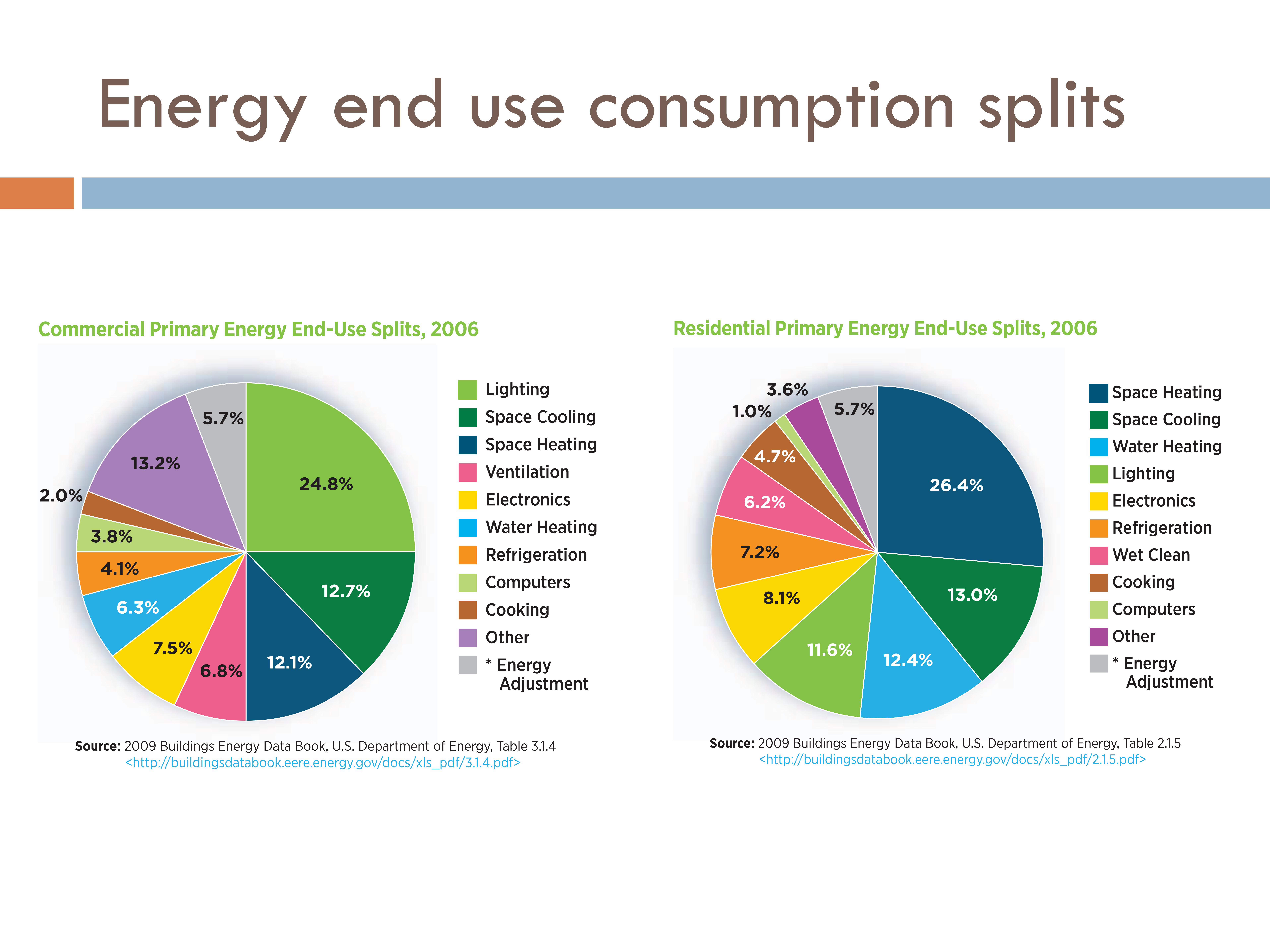
Energy end use consumption splitsProfiles of Building Sector Energy Use
Energy Use in Commercial Buildings The way energy is used in a commercial buildings has a large ef-fect on energy efficiency strategies. The most important energy end-use across the stock of commercial buildings is lighting, which accounts for one-quarter of total primary energy use.
Heating and cooling are next in importance, each with about one-seventh of the total. Equal in magnitude—though not well-defined by the U.S. DOE Energy Information Administration—is an aggregate category of miscellaneous “other uses,” such as service station equipment, ATM machines, medical equipment and telecommunications equipment. Ventilation uses another 7% of energy, making HVAC as a whole the largest user of en-ergy in commercial buildings at nearly 32%.
Water heating and office equipment (not counting personal computers) use similar amounts of energy (6%–7.5%), and re-frigeration, computer use and cooking consuming the least.
Energy Use in Residential Buildings Space heating comprises the largest energy use in a home, at one quarter—almost twice any other end use. Space cooling, water heating and lighting all use roughly the same percentage of energy in a home (12%–13%), followed by another set of uses —electronics, refrigeration and wet cleaning—sharing similar lev-els of use from 6% to 8%.
16 U.S. DEPARTMENT OF ENERGY
Figure 17 Commercial Primary Energy End-Use Splits, 2006
24.8%
12.7%
12.1% 6.8%
2.0%
13.2%
6.3%
5.7%
4.1%
3.8%
7.5%
Lighting Space Cooling Space Heating Ventilation Electronics Water Heating Refrigeration Computers Cooking Other * Energy Adjustment
Source: 2009 Buildings Energy Data Book, U.S. Department of Energy, Table 3.1.4 <http://buildingsdatabook.eere.energy.gov/docs/xls_pdf/3.1.4.pdf>
* Energy adjustment U.S. Department of Energy, Energy Information Administration uses to adjust for discrepencies between data sources. Energy attributed to the commercial buildings sector, but not directly to any specific end-use.
Figure 18 Residential Primary Energy End-Use Splits, 2006
26.4%
13.0%
12.4%11.6%
1.0%
8.1%
3.6% 5.7%
7.2%
6.2%
4.7%
Space Heating Space Cooling Water Heating Lighting Electronics Refrigeration Wet Clean Cooking Computers Other * Energy Adjustment
Source: 2009 Buildings Energy Data Book, U.S. Department of Energy, Table 2.1.5 <http://buildingsdatabook.eere.energy.gov/docs/xls_pdf/2.1.5.pdf>
* Energy adjustment U.S. Department of Energy, Energy Information Administration uses to adjust for discrepencies between data sources. Energy attributed to the residential buildings sector, but not directly to any specific end-use.
Profiles of Building Sector Energy Use
Energy Use in Commercial Buildings The way energy is used in a commercial buildings has a large ef-fect on energy efficiency strategies. The most important energy end-use across the stock of commercial buildings is lighting, which accounts for one-quarter of total primary energy use.
Heating and cooling are next in importance, each with about one-seventh of the total. Equal in magnitude—though not well-defined by the U.S. DOE Energy Information Administration—is an aggregate category of miscellaneous “other uses,” such as service station equipment, ATM machines, medical equipment and telecommunications equipment. Ventilation uses another 7% of energy, making HVAC as a whole the largest user of en-ergy in commercial buildings at nearly 32%.
Water heating and office equipment (not counting personal computers) use similar amounts of energy (6%–7.5%), and re-frigeration, computer use and cooking consuming the least.
Energy Use in Residential Buildings Space heating comprises the largest energy use in a home, at one quarter—almost twice any other end use. Space cooling, water heating and lighting all use roughly the same percentage of energy in a home (12%–13%), followed by another set of uses —electronics, refrigeration and wet cleaning—sharing similar lev-els of use from 6% to 8%.
16 U.S. DEPARTMENT OF ENERGY
Figure 17 Commercial Primary Energy End-Use Splits, 2006
24.8%
12.7%
12.1% 6.8%
2.0%
13.2%
6.3%
5.7%
4.1%
3.8%
7.5%
Lighting Space Cooling Space Heating Ventilation Electronics Water Heating Refrigeration Computers Cooking Other * Energy Adjustment
Source: 2009 Buildings Energy Data Book, U.S. Department of Energy, Table 3.1.4 <http://buildingsdatabook.eere.energy.gov/docs/xls_pdf/3.1.4.pdf>
* Energy adjustment U.S. Department of Energy, Energy Information Administration uses to adjust for discrepencies between data sources. Energy attributed to the commercial buildings sector, but not directly to any specific end-use.
Figure 18 Residential Primary Energy End-Use Splits, 2006
26.4%
13.0%
12.4%11.6%
1.0%
8.1%
3.6% 5.7%
7.2%
6.2%
4.7%
Space Heating Space Cooling Water Heating Lighting Electronics Refrigeration Wet Clean Cooking Computers Other * Energy Adjustment
Source: 2009 Buildings Energy Data Book, U.S. Department of Energy, Table 2.1.5 <http://buildingsdatabook.eere.energy.gov/docs/xls_pdf/2.1.5.pdf>
* Energy adjustment U.S. Department of Energy, Energy Information Administration uses to adjust for discrepencies between data sources. Energy attributed to the residential buildings sector, but not directly to any specific end-use.

Building Energy UseCommercial Consumption by Type
Source: WBCSD 2008

Cooling Tower
Chiller
Chilled Water Loop
Chilled Water
Cold Water
Evaporator
CondenserExpa
nsio
n V
alve
Com
pres
sor
Bypass Pipe
Bypass Pipe
Splitter
Splitter
Mixer
Mixer
Plant Loop Supply Side
Plant Loop Demand Side
Pum
p
Bypass PipeMixer
Splitter
Pump
Supply Outlet Pipe
Chilled Water Condenser Loop
Fan
Perimeter Zone Core ZonePeople, Lights & Plugs People, Lights & Plugs
Cooling Coil
Zone Splitter
Zone Mixer
Outside Air Mixer
Hot Water LoopBoiler
PumpBypass Pipe
BypassMixer
Splitter
Plant Loop Supply Side
Plant Loop Demand Side
ß Single Duct VAV
Air System
ß Reheat Coil

Large Central System Equipment

Retail System With Rooftop Units

Packaged Rooftop Unit (RTU)

Central System for Midsize Building

Packaged System for Midsize Buildings

Building-to-Grid Integration through CommercialBuilding Portfolios Participating in Energy and
Frequency Regulation Markets
Gregory S. Pavlak & Gregor P. Henze
University of Colorado Boulder
April 15, 2015

Building-to-Grid Integration through CommercialBuilding Portfolios Participating in Energy and
Frequency Regulation Markets
Gregory S. Pavlak & Gregor P. Henze
University of Colorado Boulder
April 15, 2015

Building-to-Grid Integration through CommercialBuilding Portfolios Participating in Energy and
Frequency Regulation Markets
Gregory S. Pavlak & Gregor P. Henze
University of Colorado Boulder
April 15, 2015

Motivation Modeling Multi-Market Multi-Building Portfolio Conclusions
Section 1
Motivation

Motivation Modeling Multi-Market Multi-Building Portfolio Conclusions
The Opportunity for Efficiency in Buildings
IEA: 32% of global final delivered energy [16].
more than any other sector
EIA: building energy demand projected to increase at 1.6%/year [7].
faster than any other sector
PNNL: save 1 quad primary energy through improved control [3].
6% of 2002 U.S. commercial building primary energy consumption
NREL: 50% net site energy savings over ASHRAE 90.1-2004 [15].
Achieved through holistic integration of efficiency measures

Motivation Modeling Multi-Market Multi-Building Portfolio Conclusions
Energy in Transition
IEA: global electricity demand growth projected at ≈ 2%/ year [1].
more than any other final form of energy (2011 to 2035)
U.S. consumed 78 quadsof fossil (82%) in 2012.
U.S. consumed 17 quadsof nuclear and renewables(18%) in 2012 [6].
Sustainability seems tonecessitate transitioning tomore renewables.
Biomass = 71%
Solar = 4%Geothermal = 4%
Wind = 22%
Petroleum
Coal
Natural Gas
NuclearHydro
Non−Hydro0
20
40
60
80
Fossil Nuclear Renewable
Ener
gy C
onsu
mpt
ion
[qua
drilli
on B
TU]
Motivation Modeling Multi-Market Multi-Building Portfolio Conclusions
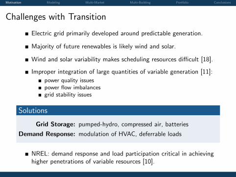
Challenges with Transition
Electric grid primarily developed around predictable generation.
Majority of future renewables is likely wind and solar.
Wind and solar variability makes scheduling resources difficult [18].
Improper integration of large quantities of variable generation [11]:
power quality issuespower flow imbalancesgrid stability issues
Solutions
Grid Storage: pumped-hydro, compressed air, batteries
Demand Response: modulation of HVAC, deferrable loads
NREL: demand response and load participation critical in achievinghigher penetrations of variable resources [10].

Motivation Modeling Multi-Market Multi-Building Portfolio Conclusions
Electricity System Overview
Continuously balance supply and demand
Diurnal load patterns caused by human activity and weather effects
Day-ahead energy market involves least-cost scheduling of base load,load following, and peaking plants → time dependent energy price
Ancillary services: frequency regulation, voltage control, and reserves
4
Co-optimization presents significant challenges for loads supplying ancillary services and especially spinning reserve. As discussed above, a critical reason some loads are better suited to supplying spinning reserve rather than peak reduction is because load response duration is limited. Co-optimization can extend the response duration unacceptably and force the load to withdraw from the market, harming power system reliability.
Co-optimization (also called joint optimization, simultaneous optimization, or rational buying) minimizes the total cost of energy, regulation, and contingency reserves by allowing the substitution of “higher value” services for “lower value” services. If a generator offers spinning reserve at $8/MW-hr, for example, and other generators are offering replacement reserve at $12/MW-hr the co-optimizer will use the spinning reserve resource for replacement reserve (instead of the replacement reserve offered) and pay it the spinning reserve clearing price. Co-optimization has many benefits. It encourages generators to bid in with their actual costs for energy and each of the ancillary services. When they do so the co-optimizer is able to simultaneously minimize overall system costs and maximize individual generator profits.
Unfortunately, co-optimization can effectively bar responsive loads as well as emissions-limited generators and water-limited hydro generators from offering to provide ancillary services.
Fundamentally the problem is that the co-optimizer is unable to deal with a rising cost curve. Many responsive loads differ from most generators in that the cost of response rises with response duration. An air conditioning load, for example, incurs almost no cost when it provides a ten minute interruption but incurs unacceptable costs when it provides a six hour interruption. Conversely a generator typically incurs startup and shutdown costs even for short responses but only has ongoing fuel costs associated with its response duration. In fact, many generators have minimum run times and minimum shutdown times. This low-cost-for-short-duration-response (coupled with fast response speed) makes some responsive loads ideal for providing spinning reserve but less well suited for providing energy response or peak reduction. A generator benefits economically when response duration is extended but a load is hurt. The co-optimizer assumes that all offering entities behave like generators and benefit from longer response.
Unfortunately current market rules in New York and New England let the ISOs dispatch capacity assigned to reserves for economic reasons as well as reliability purposes. As long as the ISO has enough spinning and non-spinning reserve capacity to cover contingencies, it will dispatch any remaining resources economically regardless of whether that capacity is labeled as contingency reserve or not. Ancillary service and energy suppliers are automatically co-optimized.
This policy works well for most generators but causes severe problems for loads that need to limit the duration or frequency of their response to occasional contingency conditions. Loads can submit very high energy bids in an
attempt to be the last resource called but this is still no guarantee that they will not be used as a multi-hour energy resource. Submitting a high cost energy bid also means that the load will be used less frequently for contingency response than is economically optimal. Price caps on energy bids further limit the ability of the loads to control how long they are deployed for.
Fortunately there is a simple solution. California had this problem with their rational buyer but changed their market rules and now allows resources to flag themselves as available for contingency response only. PJM allows resources to establish different prices for each service and energy providing a partial solution. ERCOT does not have the problem because most energy is supplied through bilateral arrangements that the ISO is not part of; energy and ancillary service markets are separate. Possibly as a consequence half of ERCOT’s contingency response comes from responsive load (the maximum currently allowed) while no loads offer to supply balancing energy.
B. Some Loads May Be Able To Provide Better Regulation Than Generators
Regulation, the minute-to-minute varying of generation or consumption at the system operator’s command in order to maintain the control area’s generation/load balance, is the most difficult ancillary service for loads to provide. Automatic generation control (AGC) commands are typically sent from the system operator to the regulating generators about every four seconds (Figure 6). Regulation is also the most expensive ancillary service so it may be the most attractive service to sell for loads that are capable of supplying it.
Fig. 6. Regulation provides the minute-to-minute balancing of generation and load.
Some loads may have the inherent capability to provide
regulation. Loads that are electronically controlled potentially could follow automatic generation control commands. Loads with large adjustable speed drives or solid state power supplies are candidates. Product quality must be independent of the rate of electricity consumption to allow the power system operator to adjust the load’s consumption. Energy efficiency can be impacted by the rate of electricity consumption. Efficiency reductions simply impact the cost of
15000
17500
20000
22500
25000
0:00 4:00 8:00 12:00 16:00 20:00 0:00
Sys
tem
Lo
ad (
MW
)
22200
22250
22300
22350
22400
8:00 8:15 8:30 8:45 9:00
Regulation
15000
17500
20000
22500
25000
0:00 4:00 8:00 12:00 16:00 20:00 0:00
Sys
tem
Lo
ad (
MW
)
22200
22250
22300
22350
22400
8:00 8:15 8:30 8:45 9:00
Regulation
B. Kirby, Load Response Fundamentally Matches Power SystemReliability Requirements (2007)
5
3. Regulation
Regulation and load following (which, in competitive spot markets, are provided by the intra-hour workings of the real-time energy market) are the two services required to continuously balance generation and load under normal conditions (Kirby and Hirst 2000). Figure 4 shows the morning ramp-up decomposed into base energy, load following, and regulation. Starting at a base energy of 3566 MW, the smooth load following ramp is shown rising to 4035 MW. Regulation consists of the rapid fluctuations in load around the underlying trend, shown here on an expanded scale to the right with a ±55 MW range. Combined, the three elements serve a load that ranges from 3539 to 4079 MW during the three hours depicted. In the PJM region, New York, New England, and Ontario, regulation is a 5-min service, defined as five times the ramp rate in megawatts per minute. In Texas it is a 15-min service, and in Alberta and California it is a 10-min service. Load following and regulation ensure that, under normal operating conditions, a control area is able to balance generation and load. Regulation is the use of on-line generation, storage, or load that is equipped with automatic generation control (AGC) and that can change output quickly (MW/min) to track the moment-to-moment fluctuations in customer loads and to correct for the unintended fluctuations in generation. Regulation helps to maintain interconnection frequency, manage differences between actual and scheduled power flows between control areas, and match generation to load within the control area. Load following is the use of on-line generation, storage, or load equipment to track the intra- and inter-hour changes in customer loads. Regulation and load following characteristics are summarized in Table 2.
3000
3200
3400
3600
3800
4000
4200
7:00 AM 8:00 AM 9:00 AM 10:00 AM
Load
and
Loa
d Fo
llow
ing
(MW
)
-60
-30
0
30
60
90
120
150
Reg
ulat
ion
(MW
)
Regulation
Total Load andLoad Following
Fig. 4. Regulation is a zero-energy service that compensates for minute-to-minute fluctuations in total system load and uncontrolled generation.
B. Kirby, Frequency Regulation Basics and Trends (2004)

Motivation Modeling Multi-Market Multi-Building Portfolio Conclusions
Building-to-Grid Integration
Passive thermal storage can buffer varied HVAC operation
Optimize thermal storage operation around energy prices
Buildings can potentially supply ancillary services to the grid:
flexible loads may be more accurate, reliable, and prompt [14].potential benefits [13]:
increased system reliabilityrisk managementreduced environmental emissionsmarket power mitigationincreased system efficiencies
Optimize operations around ancillary services
Which takes priority?
co-optimize participation in energy and ancillary service markets.determine strategies that balance the severity of grid needs with thedesire for lower utility bills

Motivation Modeling Multi-Market Multi-Building Portfolio Conclusions
Optimal Control of Building Portfolios
Past work has evaluated optimal building control from an individualperspective.
Buildings are connected to the same grid.
Individual perspective may be suboptimal.
By giving the optimizer the knowledge of all unique buildingcharacteristics available within a portfolio of buildings, variousfeatures may be exploited to orchestrate an optimal combinedoperation of all portfolio members.
Hypothesis:
Diversity among building characteristics and operations creates anopportunity for synergy.
Motivation Modeling Multi-Market Multi-Building Portfolio Conclusions
Methodology and Organization
1 Motivation
2 Modeling
3 Multi-Market
4 Multi-Building
5 Portfolio
6 Conclusions

Motivation Modeling Multi-Market Multi-Building Portfolio Conclusions
Section 2
Modeling

Motivation Modeling Multi-Market Multi-Building Portfolio Conclusions
Introduction to Model Predictive ControlExplicit system model used to predict future plant dynamics
High-level MPC (setpoints) vs. low-level MPC (tracking)
Performance oriented formulation (energy, comfort, emissions)
Incorporation of various constraints (state, action, and plant)
Moving horizon implementation
(Fig. by Gregor Henze)
Motivation Modeling Multi-Market Multi-Building Portfolio Conclusions
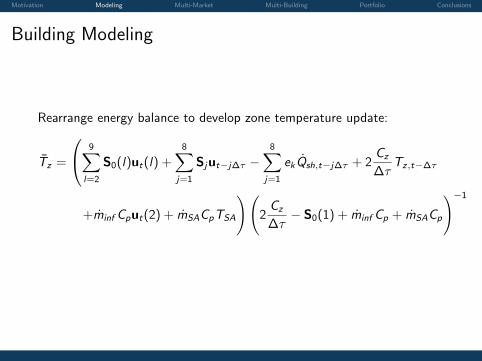
Building Modeling
Rearrange energy balance to develop zone temperature update:
Tz =
9∑l=2
S0(l)ut(l) +8∑
j=1
Sjut−j∆τ −8∑
j=1
ekQsh,t−j∆τ + 2Cz
∆τTz,t−∆τ
+minf Cput(2) + mSACpTSA
)(2Cz
∆τ− S0(1) + minf Cp + mSACp
)−1

Motivation Modeling Multi-Market Multi-Building Portfolio Conclusions
Retail Building
Vintage: 1980
Floor Area: 2294 m2
U-value: 0.418 W/(m2 K)
ACH: 1.01 hour−1
Glazing: 7%
LPD: 32.3 W/m2
EPD: 5.23 W/m2
Occ. Density: 7.11 m2/person
HVAC: CV DX RTU
!!!!!!
ZONE!
SA!
Economizer! DX!Cooling!Coil!
Gas!Hea9ng!Coil!
CV!Fan!
RA!
OA!

Motivation Modeling Multi-Market Multi-Building Portfolio Conclusions
Medium Office Building
Vintage: 2001
Floor Area: 14240 m2
U-value: 0.334 W/(m2 K)
ACH: 0.13 hour−1
Glazing: 40%
LPD: 7.16 W/m2
EPD: 4.5 W/m2
Occ. Density: 18.58 m2/person
HVAC: DX VAV !!!!!!
ZONE!
SA
Air!Mixer!
DX!Cooling!Coil!
Hea5ng!Coil!
VAV!Fan!
RA
DOAS!Supply!Fan!
DOAS!Exhaust!Fan!
OA
Exhaust
Motivation Modeling Multi-Market Multi-Building Portfolio Conclusions
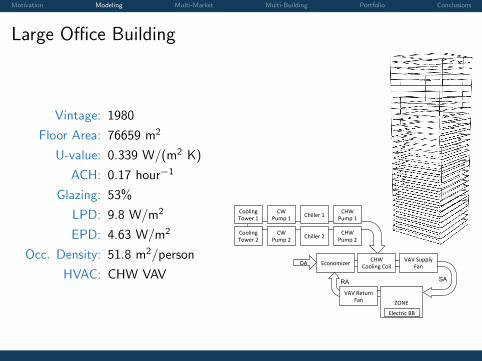
Large Office Building
Vintage: 1980
Floor Area: 76659 m2
U-value: 0.339 W/(m2 K)
ACH: 0.17 hour−1
Glazing: 53%
LPD: 9.8 W/m2
EPD: 4.63 W/m2
Occ. Density: 51.8 m2/person
HVAC: CHW VAV!!!!!!
ZONE!
SA
Economizer! CHW!Cooling!Coil!
VAV!Supply!Fan!
RA
OA!
Cooling!Tower!1!
Cooling!Tower!2!
Chiller!1!
Chiller!2!
CW!Pump!1!
CW!Pump!2!
CHW!Pump!2!
CHW!Pump!1!
Electric!BB!
VAV!Return!Fan!

Motivation Modeling Multi-Market Multi-Building Portfolio Conclusions
Retail Model Validation
11p RC network
4760 4780 4800 4820 4840 4860 4880 4900 4920 494016
18
20
22
24
26
28
30
Tem
pera
ture
(C)
Retail Model Validation:Zone Temperature − Precool
setpoint EnergyPlus Simplified
4760 4780 4800 4820 4840 4860 4880 4900 4920 4940
1000
2000
3000
4000
Cumulative Temperature (C)
Time (hours)
Tem
pera
ture
(C)
RMSE = 0.24MBE = −0.04Cum. % Err = −0.19%
EnergyPlusSimplified
4760 4780 4800 4820 4840 4860 4880 4900 4920 49400
20
40
60
80
100
120
En
erg
y (k
Wh
)
Retail Model Validation:HVAC Electric Consumption ! Precool
EnergyPlus Simplified
4760 4780 4800 4820 4840 4860 4880 4900 4920 49400
2000
4000
6000
Cumulative Energy (kWh)
Time (hours)
En
erg
y (k
Wh
)
RMSE = 6.49MBE = !0.04Cum. % Err = !0.11%
EnergyPlusSimplified

Motivation Modeling Multi-Market Multi-Building Portfolio Conclusions
Medium Office Model Validation
5p RC network
5260 5280 5300 5320 5340 5360 5380 5400 5420 544020
21
22
23
24
25
26
27
28
Mean A
ir T
em
p (
C)
Medium Office Model Validation:Zone Temperature ! Precool
Setpoint EnergyPlus Simplified
5260 5280 5300 5320 5340 5360 5380 5400 5420 5440
1000
2000
3000
4000
Cumulative Mean Air Temp (C)
Time (hours)
Mean A
ir T
em
p (
C)
RMSE = 0.52MBE = 0.35Cum. % Err = 1.42%
EnergyPlusSimplified
5260 5280 5300 5320 5340 5360 5380 5400 5420 54400
100
200
300
400
500
600
En
erg
y (k
Wh
)
Medium Office Model Validation:HVAC Electric Consumption ! Precool
EnergyPlus Simplified
5260 5280 5300 5320 5340 5360 5380 5400 5420 54400
5000
10000
15000
Cumulative Energy (kWh)
Time (hours)
En
erg
y (k
Wh
)
RMSE = 28.18MBE = 9.77Cum. % Err = 10.81%
EnergyPlusSimplified

Motivation Modeling Multi-Market Multi-Building Portfolio Conclusions
Large Office Model Validation
21p RC network
4740 4760 4780 4800 4820 4840 4860 4880 4900 4920 494018
20
22
24
26
28
30
32
Tem
pera
ture
(C)
Large Office Model Validation:Zone Temperature − Precool
setpoint EnergyPlus Simplified
4740 4760 4780 4800 4820 4840 4860 4880 4900 4920 4940
1000
2000
3000
4000
5000
Cumulative Temperature (C)
Time (hours)
Tem
pera
ture
(C)
RMSE = 0.39MBE = 0.04Cum. % Err = 0.14%
EnergyPlusSimplified
4740 4760 4780 4800 4820 4840 4860 4880 4900 4920 49400
500
1000
1500
2000
2500
3000
3500
4000
Elec
tric
Con
sum
ptio
n (k
Wh)
Large Office Model Validation:HVAC Electric Consumption − Precool
EnergyPlus Simplified
4740 4760 4780 4800 4820 4840 4860 4880 4900 4920 49400
0.5
1
1.5
2x 10⁵ Cumulative Electric Consumption (kWh)
Time (hours)Elec
tric
Con
sum
ptio
n (k
Wh)
RMSE = 267.54MBE = −14.50Cum. % Err = −1.43%
EnergyPlusSimplified
Motivation Modeling Multi-Market Multi-Building Portfolio Conclusions
Section 3
Multi-Market

Motivation Modeling Multi-Market Multi-Building Portfolio Conclusions
Background
Well established for traditional generation resources
Typically linear models solved with DP or MILP [5, 9, 2]
Vehicle-to-grid optimal charging algorithms [17]
Linear models solved using LP
Frequency regulation in commercial buildings:
Zhao et al. FR via duct SP and zone setpoint modulation [19]Hao et al. FR via direct fan speed modulation [12]
Challenges of multi-market scheduling in buildings
occupant thermal, visual, and IAQ constraintspassive thermal storage vs. direct electricHVAC system capacity constraints and staging
Whole-building energy model perturbation approach proposed

Motivation Modeling Multi-Market Multi-Building Portfolio Conclusions
FR Estimation
An illustrative example: How much FR at 13:00?
Baseline setpoint of 23 ◦C
Fans 50%, DX Coil: On-On-Cyc-Off, 85% Occupied
22.0
22.5
23.0
23.5
24.0
Zone
Tem
pera
ture
[°C
]
350
400
450
500
550
600
06:00 09:00 12:00 15:00 18:00
Faci
lity
Elec
tric
[kW
]

Motivation Modeling Multi-Market Multi-Building Portfolio Conclusions
FR Estimation
●●
●●−100
−50
0
50
100
22.5 23.0 23.5Zone Temperature [°C]
Δ P
ower
[kW
]
CoolingStagesON● 2
34
Group power response based on number of active cooling stages.
Max: ±100 kW, 22.3 ◦C to 23.8 ◦C

Motivation Modeling Multi-Market Multi-Building Portfolio Conclusions
FR Estimation
Occupied Tmax
Occupied Tmin
Reg. DownReg. Up
22
23
24
25
26
27Zo
ne T
empe
ratu
re [°
C]
Baseline Setpoint Temp. Limits Zone Temp.
Regulating Band
Reg. Down
Reg. Up−50
0
50
06:00 09:00 12:00 15:00 18:00
Δ P
ower
[kW
] Regulating Band
Repeat perturbation for desired hours (9am to 4pm in this example).

Motivation Modeling Multi-Market Multi-Building Portfolio Conclusions
Multi-Market Optimization
Problem:min J (~x) s.t.: ~x ∈ [~xmin, ~xmax ]
Cost function:
J (~x) = Ecost + Pdemand − Rreg
Energy cost:
Ecost =
tCH∑t=1
rDA (t)Euse (t)
Demand penalty:
Pdemand = max [M (max (ElecDemandpeak)− TDL) , 0]
Regulation revenue:
Rreg =
tCH∑t=1
∆power (t) rreg (t)

Motivation Modeling Multi-Market Multi-Building Portfolio Conclusions
Multi-Market Optimization Overview
simulate(~x + �1) . . . simulate(~x + �n)
simulate(~x)
objfun
optimizer
J (~x)
~xPdemand
Energy
�power
FR estimation
chiller(~x + �1, X) . . . chiller(~x + �n, X)
simulate(~x)
objfun
optimizer
J (~x)
~x
Pdemand
X
Energy
�power
FR estimation
1
Perturbations limited to those that do not increase the demand penalty.

Motivation Modeling Multi-Market Multi-Building Portfolio Conclusions
Medium Office ResultsLow Target Demand Limit
●
●
●
●
●
●
●
●
●
●●
●
●
●●
● ● ●
●● ●
Occupied Tmax
Occupied Tmin
On−Peak:
$5.50/kWdemand penalty
for all kW's> 325 kW
22
24
26Zo
ne T
empe
ratu
re [°
C]
NSU Set.NSU Temp.OPT+FR Set.OPT+FR Temp. OPT+FR ● OPT Temp.
●
● ●
●● ●
●
●
●
●
●
●
●● ●
● ● ●
●●
●
0
100
200
300
400
500
Elec
tric
Dem
and
[kW
]
NSU Power OPT+FR Power ● OPT Power OPT+FR
050
100150200
03:00 06:00 09:00 12:00 15:00 18:00
Pric
e [$
/MW
h] DA Energy Regulation
Available 5/9 hours
±8 kW to ±60 kW
$12 reg. revenue
38% → 39.5%

Motivation Modeling Multi-Market Multi-Building Portfolio Conclusions
Medium Office ResultsLow Target Demand Limit
Summary:
Available 5/9 hours
±8 kW to ±60 kW
$12 reg. revenue
38% → 39.5%
●
●
●
●
●
●
●
●
●
●●
●
●
●●
● ● ●
●● ●
Occupied Tmax
Occupied Tmin
On−Peak:
$5.50/kWdemand penalty
for all kW's> 325 kW
22
24
26
Zone
Tem
pera
ture
[°C
]
NSU Set.NSU Temp.OPT+FR Set.OPT+FR Temp. OPT+FR ● OPT Temp.
●
● ●
●● ●
●
●
●
●
●
●
●● ●
● ● ●
●●
●
0
100
200
300
400
500
Elec
tric
Dem
and
[kW
]
NSU Power OPT+FR Power ● OPT Power OPT+FR
050
100150200
03:00 06:00 09:00 12:00 15:00 18:00
Pric
e [$
/MW
h] DA Energy Regulation
Motivation Modeling Multi-Market Multi-Building Portfolio Conclusions
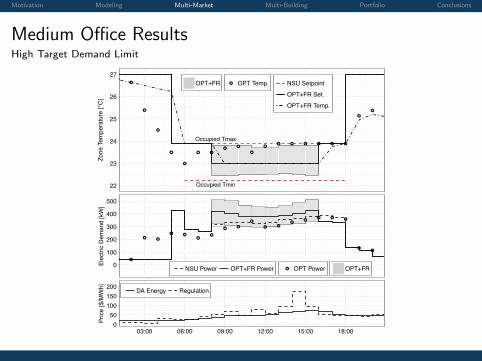
Medium Office ResultsHigh Target Demand Limit
●●
●
●
●
●
● ●●
●
●
●● ● ● ● ● ●
●
● ●
Occupied Tmax
Occupied Tmin22
23
24
25
26
27
Zone
Tem
pera
ture
[°C]
OPT+FR ● OPT Temp. NSU SetpointOPT+FR Set.OPT+FR Temp.
● ●
● ●
● ●●
●
●●
●
● ●●
●● ● ●
●●
●
0
100
200
300
400
500
Elec
tric
Dem
and
[kW
]
NSU Power OPT+FR Power ● OPT Power OPT+FR
050
100150200
03:00 06:00 09:00 12:00 15:00 18:00
Price
[$/M
Wh] DA Energy Regulation
Available 8/9 hours
277 kWh > OPT
$23 > energy expense
±85 kW on average
$56 reg. revenue
2.3% → 15.7%

Motivation Modeling Multi-Market Multi-Building Portfolio Conclusions
Medium Office ResultsHigh Target Demand Limit
Summary:
Available 8/9 hours
277 kWh > OPT
$23 > energy expense
±85 kW on average
$56 reg. revenue
2.3% → 15.7%
●●
●
●
●
●
● ●●
●
●
●● ● ● ● ● ●
●
● ●
Occupied Tmax
Occupied Tmin22
23
24
25
26
27
Zone
Tem
pera
ture
[°C]
OPT+FR ● OPT Temp. NSU SetpointOPT+FR Set.OPT+FR Temp.
● ●
● ●
● ●●
●
●●
●
● ●●
●● ● ●
●●
●
0
100
200
300
400
500
Elec
tric
Dem
and
[kW
]
NSU Power OPT+FR Power ● OPT Power OPT+FR
050
100150200
03:00 06:00 09:00 12:00 15:00 18:00
Price
[$/M
Wh] DA Energy Regulation

Motivation Modeling Multi-Market Multi-Building Portfolio Conclusions
Chiller Power Response
CHW Supply Temp (C)
Qev
ap/Q
rate
d
4 5 6 7 8 9 100
0.1
0.2
0.3
0.4
0.5
0.6
0.7
0.8
0.9
1
P/Pr
ated
0.2
0.3
0.4
0.5
0.6
0.7
0.8
0.9
1
1.1
1.2
Condenser water temperature is a constant 26.7 ◦C.
State 1 State 2 State 3Tchw,supply 7 ◦C 6 ◦C 6 ◦CTchw,return 9.1 ◦C 9.1 ◦C 8.1 ◦CCOP 3.18 3.52 3.13

Motivation Modeling Multi-Market Multi-Building Portfolio Conclusions
Chiller Power Response
X = 7Y = 0.3069Z = 0.425
CHW Supply Temp (C)
Qev
ap/Q
rate
d
4 5 6 7 8 9 100
0.1
0.2
0.3
0.4
0.5
0.6
0.7
0.8
0.9
1
P/Pr
ated
0.2
0.3
0.4
0.5
0.6
0.7
0.8
0.9
1
1.1
1.2
1
State 1 State 2 State 3Tchw,supply 7 ◦C 6 ◦C 6 ◦CTchw,return 9.1 ◦C 9.1 ◦C 8.1 ◦CCOP 3.18 3.52 3.13

Motivation Modeling Multi-Market Multi-Building Portfolio Conclusions
Chiller Power Response
X = 7Y = 0.3069Z = 0.425
X = 6Y = 0.4531Z = 0.5661
CHW Supply Temp (C)
Qev
ap/Q
rate
d
4 5 6 7 8 9 100
0.1
0.2
0.3
0.4
0.5
0.6
0.7
0.8
0.9
1
P/Pr
ated
0.2
0.3
0.4
0.5
0.6
0.7
0.8
0.9
1
1.1
1.2
1
2
State 1 State 2 State 3Tchw,supply 7 ◦C 6 ◦C 6 ◦CTchw,return 9.1 ◦C 9.1 ◦C 8.1 ◦CCOP 3.18 3.52 3.13

Motivation Modeling Multi-Market Multi-Building Portfolio Conclusions
Chiller Power Response
CHW Supply Temp (C)
Qev
ap/Q
rate
d
X = 7Y = 0.3069Z = 0.425
X = 6Y = 0.4531Z = 0.5661
X = 6Y = 0.3069Z = 0.4315
4 5 6 7 8 9 100
0.1
0.2
0.3
0.4
0.5
0.6
0.7
0.8
0.9
1
P/Pr
ated
0.2
0.3
0.4
0.5
0.6
0.7
0.8
0.9
1
1.1
1.2
13
2
State 1 State 2 State 3Tchw,supply 7 ◦C 6 ◦C 6 ◦CTchw,return 9.1 ◦C 9.1 ◦C 8.1 ◦CCOP 3.18 3.52 3.13

Motivation Modeling Multi-Market Multi-Building Portfolio Conclusions
Section 4
Multi-Building

Motivation Modeling Multi-Market Multi-Building Portfolio Conclusions
Multi-Building Optimization
Need to extend MPC environment originally developed by Corbin et al. [8]
Multi-building is a generalization of single building problem.
1 Initialization
2 Optimization
3 Execution

Motivation Modeling Multi-Market Multi-Building Portfolio Conclusions
Multi-Building OptimizationInitialization
(1) load(globalParams)(2) for n = 1 to N(3)
(4) load(localParams(n));(5) load(weather(n));(6) load(utilityData(n));(7) load(Model(n));(8) warmUp(Model(n));(9)
(10) end
1
Bldg 1
Bldg 2
Bldg N
...
1
Motivation Modeling Multi-Market Multi-Building Portfolio Conclusions
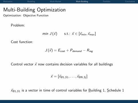
Multi-Building OptimizationOptimization: Objective Function
Problem:
min J (~x) s.t.: ~x ∈ [~xmin, ~xmax ]
Cost function:
J (~x) = Ecost + Pdemand − Rreg
Control vector ~x now contains decision variables for all buildings
~x = [~xB1,S1, . . . , ~xBN,Sj ]
~xB1,S1 is a vector in time of control variables for Building 1, Schedule 1

Motivation Modeling Multi-Market Multi-Building Portfolio Conclusions
Multi-Building OptimizationOptimization: Overview
complete?
J (~x)
~x
[~xB1,S1, . . . , ~xBN,Sj ]
[~xB1,S1, . . . , ~xB1,Sh] [~xB2,S1, . . . , ~xB2,Si] [~xBN,S1, . . . , ~xBN,Sj ]
Bldg 1 Bldg 2 Bldg N. . .
. . .
. . .ROM E+ ROM
FRFR
out1 (~x, �) out2 (~x, �) outN (~x)
Determine Optimal FR Calc. Demand Penalty Calc. Cost
Objective FunctionRreg + Pdemand + Ecost
OPT+FR 1
OPT+FR 2
OPT N
no yes ...
1

Motivation Modeling Multi-Market Multi-Building Portfolio Conclusions
Section 5
Portfolio
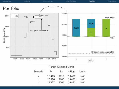
Motivation Modeling Multi-Market Multi-Building Portfolio Conclusions
Portfolio
Target Demand Limit
Scenario Rs Ls (RL)p Units
a 16 419 3013 19 432 kWb 16 826 2606 19 432 kWc 17 227 2205 19 432 kW
TDL
Min. peak achievable
5000
10000
15000
20000
03:00 06:00 09:00 12:00 15:00 18:00 21:00
Elec
tric
Dem
and
[kW
]
NSU
120R
120R
L
L
TDL
Minimum peak achievable
Max. NSU
18500
19000
19500
20000
20500
a b cScenario
1

Motivation Modeling Multi-Market Multi-Building Portfolio Conclusions
Scenario a: RetailNo Frequency Regulation
Occupied Tmax
Occupied Tmin
● ● ● ● ● ● ● ● ● ● ● ● ● ● ● ● ● ● ● ● ● ●● ●
●●
●●
● ● ●●
● ● ● ● ● ● ● ● ● ● ● ● ●●
●●
On−Peak
15
20
25
30
Zone
Tem
pera
ture
[°C
]
● ● ● ● ● ● ●
●
●
●● ●
●● ● ● ● ●
●
●
●
●
● ●● ● ● ● ● ● ●
●
●
●
● ●
●
●●
●●
●
●
●
●
●
● ●
TDL
0
5000
10000
15000
03:00 06:00 09:00 12:00 15:00 18:00 21:00
Elec
tric
Con
sum
ptio
n [k
Wh]
● ●NSU Rp NSU Rs OPT Rp OPT Rs
Rp
Rs
Rp
Rs
$0 $5,000 $10,000Energy Cost [$]
Sim
ulat
ion
Stat
s
0 100 200Energy Use [MWh]
NSU
OPT
$0Reg. Rev. [$]
TDL
Min. peak achievable
5000
10000
15000
20000
03:00 06:00 09:00 12:00 15:00 18:00 21:00
Elec
tric
Dem
and
[kW
]
NSU
120R
120R
L
L
TDL
Minimum peak achievable
Max. NSU
18500
19000
19500
20000
20500
a b cScenario
a b c

Motivation Modeling Multi-Market Multi-Building Portfolio Conclusions
Scenario a: Large OfficeNo Frequency Regulation
Occupied Tmax
Occupied Tmin
● ● ● ● ● ●
●
● ● ● ● ● ● ● ● ● ● ●
●● ● ● ● ●
● ●● ● ● ●
●
● ● ● ● ● ● ● ● ● ● ●
●
● ● ● ● ●
On−Peak
22
24
26
28
30
Zone
Tem
pera
ture
[°C
]
TDL
● ● ● ● ● ●
●
●
● ● ● ●●
● ● ●● ●
● ● ●● ● ●
●● ● ● ● ●
●
●
● ●● ●
●
●●
●
● ●
● ●●
● ● ●
0
1000
2000
3000
4000
03:00 06:00 09:00 12:00 15:00 18:00 21:00
Elec
tric
Con
sum
ptio
n [k
Wh]
● ●NSU Lp NSU Ls OPT Lp OPT Ls
Lp
Ls
Lp
Ls
$0 $900 $1,800Energy Cost [$]
Sim
ulat
ion
Stat
s
0 10 20 30 40 50Energy Use [MWh]
NSU
OPT
$0Reg. Rev. [$]
TDL
Min. peak achievable
5000
10000
15000
20000
03:00 06:00 09:00 12:00 15:00 18:00 21:00
Elec
tric
Dem
and
[kW
]
NSU
120R
120R
L
L
TDL
Minimum peak achievable
Max. NSU
18500
19000
19500
20000
20500
a b cScenario
a b c
Motivation Modeling Multi-Market Multi-Building Portfolio Conclusions
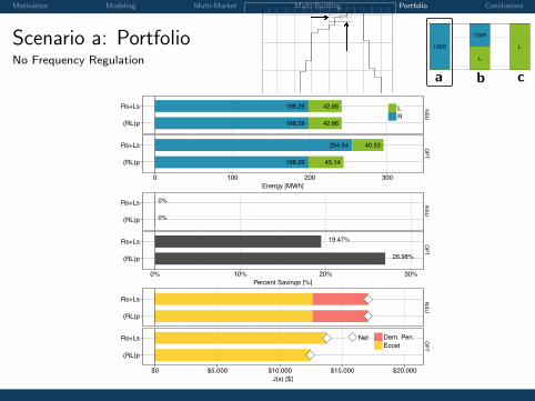
Scenario a: PortfolioNo Frequency Regulation
TDL
Min. peak achievable
5000
10000
15000
20000
03:00 06:00 09:00 12:00 15:00 18:00 21:00
Elec
tric
Dem
and
[kW
]
NSU
120R
120R
L
L
TDL
Minimum peak achievable
Max. NSU
18500
19000
19500
20000
20500
a b cScenario
a b c
198.29 42.86
198.29 42.86
198.29 45.14
254.64 40.53
(RL)p
Rs+Ls
(RL)p
Rs+Ls
NSU
OPT
0 100 200 300Energy [MWh]
LR
0%
0%
19.47%
26.98%
(RL)p
Rs+Ls
(RL)p
Rs+Ls
NSU
OPT
0% 10% 20% 30%Percent Savings [%]
(RL)p
Rs+Ls
(RL)p
Rs+Ls
NSU
OPT
$0 $5,000 $10,000 $15,000 $20,000J(x) [$]
Net Dem. Pen.Ecost

Motivation Modeling Multi-Market Multi-Building Portfolio Conclusions
Scenario a: PortfolioNo Frequency Regulation
TDL
Min. peak achievable
5000
10000
15000
20000
03:00 06:00 09:00 12:00 15:00 18:00 21:00
Elec
tric
Dem
and
[kW
]
NSU
120R
120R
L
L
TDL
Minimum peak achievable
Max. NSU
18500
19000
19500
20000
20500
a b cScenario
a b c
198.29 42.86
198.29 42.86
198.29 45.14
254.64 40.53
(RL)p
Rs+Ls
(RL)p
Rs+Ls
NSU
OPT
0 100 200 300Energy [MWh]
LR
0%
0%
19.47%
26.98%
(RL)p
Rs+Ls
(RL)p
Rs+Ls
NSU
OPT
0% 10% 20% 30%Percent Savings [%]
(RL)p
Rs+Ls
(RL)p
Rs+Ls
NSU
OPT
$0 $5,000 $10,000 $15,000 $20,000J(x) [$]
Net Dem. Pen.Ecost
!!

Motivation Modeling Multi-Market Multi-Building Portfolio Conclusions
Portfolio: RetailNo Frequency Regulation
Occupied Tmax
Occupied Tmin
● ● ● ● ● ● ● ● ● ● ● ● ● ● ● ● ● ● ● ● ● ●● ●
●●
●●
● ● ●●
● ● ● ● ● ● ● ● ● ● ● ● ●●
●●
On−Peak
15
20
25
30
Zone
Tem
pera
ture
[°C
]
● ● ● ● ● ● ●
●
●
●● ●
●● ● ● ● ●
●
●
●
●
● ●● ● ● ● ● ● ●
●
●
●
● ●
●
●●
●●
●
●
●
●
●
● ●
TDL
0
5000
10000
15000
03:00 06:00 09:00 12:00 15:00 18:00 21:00
Elec
tric
Con
sum
ptio
n [k
Wh]
● ●NSU Rp NSU Rs OPT Rp OPT Rs
Rp
Rs
Rp
Rs
$0 $5,000 $10,000Energy Cost [$]
Sim
ulat
ion
Stat
s
0 100 200Energy Use [MWh]
NSU
OPT
$0Reg. Rev. [$]
TDL
Min. peak achievable
5000
10000
15000
20000
03:00 06:00 09:00 12:00 15:00 18:00 21:00
Elec
tric
Dem
and
[kW
]
NSU
120R
120R
L
L
TDL
Minimum peak achievable
Max. NSU
18500
19000
19500
20000
20500
a b cScenario
a b c

Motivation Modeling Multi-Market Multi-Building Portfolio Conclusions
Portfolio: Large OfficeNo Frequency Regulation
Occupied Tmax
Occupied Tmin
● ● ● ● ● ●
●
● ● ● ● ● ● ● ● ● ● ●
●● ● ● ● ●
● ●● ● ● ●
●
● ● ● ● ● ● ● ● ● ● ●
●
● ● ● ● ●
On−Peak
22
24
26
28
30
Zone
Tem
pera
ture
[°C
]
TDL
● ● ● ● ● ●
●
●
● ● ● ●●
● ● ●● ●
● ● ●● ● ●
●● ● ● ● ●
●
●
● ●● ●
●
●●
●
● ●
● ●●
● ● ●
0
1000
2000
3000
4000
03:00 06:00 09:00 12:00 15:00 18:00 21:00
Elec
tric
Con
sum
ptio
n [k
Wh]
● ●NSU Lp NSU Ls OPT Lp OPT Ls
Lp
Ls
Lp
Ls
$0 $900 $1,800Energy Cost [$]
Sim
ulat
ion
Stat
s
0 10 20 30 40 50Energy Use [MWh]
NSU
OPT
$0Reg. Rev. [$]
TDL
Min. peak achievable
5000
10000
15000
20000
03:00 06:00 09:00 12:00 15:00 18:00 21:00
Elec
tric
Dem
and
[kW
]
NSU
120R
120R
L
L
TDL
Minimum peak achievable
Max. NSU
18500
19000
19500
20000
20500
a b cScenario
a b c

Motivation Modeling Multi-Market Multi-Building Portfolio Conclusions
Portfolio ResultsNo Frequency Regulation
198.29 42.86
198.29 42.86
198.29 45.14
254.64 40.53
(RL)p
Rs+Ls
(RL)p
Rs+Ls
NSU
OPT
0 100 200 300Energy [MWh]
LR
0%
0%
19.47%
26.98%
(RL)p
Rs+Ls
(RL)p
Rs+Ls
NSU
OPT
0% 10% 20% 30%Percent Savings [%]
(RL)p
Rs+Ls
(RL)p
Rs+Ls
NSU
OPT
$0 $5,000 $10,000 $15,000 $20,000J(x) [$]
Net Dem. Pen.Ecost
TDL
Min. peak achievable
5000
10000
15000
20000
03:00 06:00 09:00 12:00 15:00 18:00 21:00
Elec
tric
Dem
and
[kW
]
NSU
120R
120R
L
L
TDL
Minimum peak achievable
Max. NSU
18500
19000
19500
20000
20500
a b cScenario
a b c

Motivation Modeling Multi-Market Multi-Building Portfolio Conclusions
Portfolio ResultsNo Frequency Regulation
198.29 42.86
198.29 42.86
198.29 45.14
213.66 41.46
(RL)p
Rs+Ls
(RL)p
Rs+Ls
NSU
OPT
0 100 200 300Energy [MWh]
LR
0%
0%
24.76%
26.98%
(RL)p
Rs+Ls
(RL)p
Rs+Ls
NSU
OPT
0% 10% 20% 30%Percent Savings [%]
(RL)p
Rs+Ls
(RL)p
Rs+Ls
NSU
OPT
$0 $5,000 $10,000 $15,000 $20,000J(x) [$]
Net Dem. Pen.Ecost
TDL
Min. peak achievable
5000
10000
15000
20000
03:00 06:00 09:00 12:00 15:00 18:00 21:00
Elec
tric
Dem
and
[kW
]
NSU
120R
120R
L
L
TDL
Minimum peak achievable
Max. NSU
18500
19000
19500
20000
20500
a b cScenario
a b c

Motivation Modeling Multi-Market Multi-Building Portfolio Conclusions
Portfolio ResultsNo Frequency Regulation
198.29 42.86
198.29 42.86
198.29 45.14
198.29 49.58
(RL)p
Rs+Ls
(RL)p
Rs+Ls
NSU
OPT
0 100 200 300Energy [MWh]
LR
0%
0%
26.54%
26.98%
(RL)p
Rs+Ls
(RL)p
Rs+Ls
NSU
OPT
0% 10% 20% 30%Percent Savings [%]
(RL)p
Rs+Ls
(RL)p
Rs+Ls
NSU
OPT
$0 $5,000 $10,000 $15,000 $20,000J(x) [$]
Net Dem. Pen.Ecost
TDL
Min. peak achievable
5000
10000
15000
20000
03:00 06:00 09:00 12:00 15:00 18:00 21:00
Elec
tric
Dem
and
[kW
]
NSU
120R
120R
L
L
TDL
Minimum peak achievable
Max. NSU
18500
19000
19500
20000
20500
a b cScenario
a b c

Motivation Modeling Multi-Market Multi-Building Portfolio Conclusions
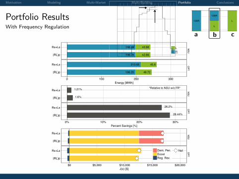
Portfolio ResultsWith Frequency Regulation
198.29 42.86
198.29 42.86
198.29 46.72
254.64 44.62
(RL)p
Rs+Ls
(RL)p
Rs+Ls
NSU
OPT
0 100 200 300Energy [MWh]
LR
1.21%
1.6%
*Relative to NSU w/o FR*
21.15%
28.44%
(RL)p
Rs+Ls
(RL)p
Rs+Ls
NSU
OPT
0% 10% 20% 30%Percent Savings [%]
(RL)p
Rs+Ls
(RL)p
Rs+Ls
NSU
OPT
$0 $5,000 $10,000 $15,000 $20,000J(x) [$]
Dem. Pen.EcostReg. Rev.
Net
TDL
Min. peak achievable
5000
10000
15000
20000
03:00 06:00 09:00 12:00 15:00 18:00 21:00
Elec
tric
Dem
and
[kW
]
NSU
120R
120R
L
L
TDL
Minimum peak achievable
Max. NSU
18500
19000
19500
20000
20500
a b cScenario
a b c
Motivation Modeling Multi-Market Multi-Building Portfolio Conclusions
Portfolio ResultsWith Frequency Regulation
198.29 42.86
198.29 42.86
198.29 46.72
213.66 45.6
(RL)p
Rs+Ls
(RL)p
Rs+Ls
NSU
OPT
0 100 200 300Energy [MWh]
LR
1.21%
1.6%
*Relative to NSU w/o FR*
26.2%
28.44%
(RL)p
Rs+Ls
(RL)p
Rs+Ls
NSU
OPT
0% 10% 20% 30%Percent Savings [%]
(RL)p
Rs+Ls
(RL)p
Rs+Ls
NSU
OPT
$0 $5,000 $10,000 $15,000 $20,000J(x) [$]
Dem. Pen.EcostReg. Rev.
Net
TDL
Min. peak achievable
5000
10000
15000
20000
03:00 06:00 09:00 12:00 15:00 18:00 21:00
Elec
tric
Dem
and
[kW
]
NSU
120R
120R
L
L
TDL
Minimum peak achievable
Max. NSU
18500
19000
19500
20000
20500
a b cScenario
a b c

Motivation Modeling Multi-Market Multi-Building Portfolio Conclusions
Portfolio ResultsWith Frequency Regulation
198.29 42.86
198.29 42.86
198.29 46.72
198.29 49.72
(RL)p
Rs+Ls
(RL)p
Rs+Ls
NSU
OPT
0 100 200 300Energy [MWh]
LR
1.21%
1.6%
*Relative to NSU w/o FR*
27.83%
28.44%
(RL)p
Rs+Ls
(RL)p
Rs+Ls
NSU
OPT
0% 10% 20% 30%Percent Savings [%]
(RL)p
Rs+Ls
(RL)p
Rs+Ls
NSU
OPT
$0 $5,000 $10,000 $15,000 $20,000J(x) [$]
Dem. Pen.EcostReg. Rev.
Net
TDL
Min. peak achievable
5000
10000
15000
20000
03:00 06:00 09:00 12:00 15:00 18:00 21:00
Elec
tric
Dem
and
[kW
]
NSU
120R
120R
L
L
TDL
Minimum peak achievable
Max. NSU
18500
19000
19500
20000
20500
a b cScenario
a b c

Motivation Modeling Multi-Market Multi-Building Portfolio Conclusions
Portfolio SummaryIn general, retail buildings were less efficient at load shifting
21% less thermal capacitance23% higher average construction U-value6x greater ACH2.6x internal gains
Energy savings over aggregated individual solutions:Scenario a: 17.5%Scenario b: 5%Scenario c: 1.6%
Percent savings summary for Portfolio:
No FR FRScenario Rs+Ls (RL)p Diff. Rs+Ls (RL)p Diff.
a -19.47% -26.98% 7.51 -21.15% -28.44% 7.29b -24.76% -26.98% 2.22 -26.20% -28.44% 2.24c -26.54% -26.98% 0.44 -27.83% -28.44% 0.60

Motivation Modeling Multi-Market Multi-Building Portfolio Conclusions
Section 6
Conclusions

Motivation Modeling Multi-Market Multi-Building Portfolio Conclusions
got synergy?
What was the nature of observed synergistic effect?
1 Synergy was dependent on individual building opt. conditions
2 Synergy was dependent on portfolio construction
3 Synergy was dependent on grid market design (i.e. demand charge)

Motivation Modeling Multi-Market Multi-Building Portfolio Conclusions
Contributions to Building-to-Grid Integration
1 Model-based method for estimating commercial building frequencyregulation capability
2 Thermal mass optimization considering ancillary service revenueopportunities along with energy price and demand
3 Centralized building portfolio optimization approach
4 Identified several opportunities for synergy among portfolios

Motivation Modeling Multi-Market Multi-Building Portfolio Conclusions
Thank you.
Questions?
Motivation Modeling Multi-Market Multi-Building Portfolio Conclusions
References I
[1] Fatih Birol, Laura Cozzi, Tim Gould, Amos Bromhead, Christian Besson, DanDorner, Marco Baroni, Pawel Olejarnik, and Timur Gul.
World Energy Outlook.
Technical report, International Energy Agency, Paris, France, 2013.
[2] Alberto Borghetti, Claudia D Ambrosio, Andrea Lodi, and Silvano Martello.
An MILP Approach for Short-Term Hydro Scheduling and Unit Commitment WithHead-Dependent Reservoir.
IEEE Transactions on Power Systems, 23(3):1115–1124, 2008.
[3] M R Brambley, Phil Haves, S C McDonald, Paul A Torcellini, D Hansen, D RHolmberg, and K W Roth.
Advanced Sensors and Controls for Building Applications : Market Assessmentand Potential R & D Pathways (PNNL-15149).
Technical Report April, Pacific Northwest National Laboratory, 2005.
[4] Nitin Chaturvedi and James E Braun.
Analytical Tools for Dynamic Building Control (ASHRAE 985-RP).
Technical Report October, Raw W. Herrick Laboratories - Purdue, 2000.

Motivation Modeling Multi-Market Multi-Building Portfolio Conclusions
References II
[5] Arthur I Cohen and S H Wan.
An Algorithm for Scheduling a Large Pumped Storage Plant.
IEEE Transactions on Power Apparatus and Systems, PAS-104(8):2099–2104,1985.
[6] John Conti, Paul Holtberg, Joseph Beamon, Sam Napolitano, A. Michael Schaal,and James T Turnure.
Annual Energy Outlook.
Technical report, U.S. Energy Information Administration, Washington, DC, 2013.
[7] John Conti, Paul Holtberg, Joseph Beamon, Sam Napolitano, A. Michael Schaal,James T Turnure, and Lynn Westfall.
International Energy Outlook.
Technical report, U.S. Energy Information Administration, Washington, DC, 2013.
[8] Charles D Corbin, Gregor P Henze, and Peter May-Ostendorp.
A model predictive control optimization environment for real-time commercialbuilding application.
Journal of Building Performance Simulation, 6(3):159–174, May 2013.

Motivation Modeling Multi-Market Multi-Building Portfolio Conclusions
References III
[9] Javier Garcıa-Gonzalez, Ernesto Parrilla, and Alicia Mateo.
Risk-averse profit-based optimal scheduling of a hydro-chain in the day-aheadelectricity market.
European Journal of Operational Research, 181(3):1354–1369, September 2007.
[10] GE Energy.
Western Wind and Solar Integration Study.
Technical Report May, National Renewable Energy Laboratory, Golden, CO, 2010.
[11] Pavlos S Georgilakis.
Technical challenges associated with the integration of wind power into powersystems.
Renewable and Sustainable Energy Reviews, 12(3):852–863, April 2008.
[12] He Hao, Anupama Kowli, Yashen Lin, Prabir Barooah, and Sean Meyn.
Ancillary Service for the Grid via Control of Commercial Building HVAC Systems.
In American Control Conference, pages 1–6, Washington, DC, 2013.

Motivation Modeling Multi-Market Multi-Building Portfolio Conclusions
References IV
[13] David Kathan.
Policy and Technical Issues Associated with ISO Demand Response Programs.
Technical Report July, The National Association of Regulatory UtilityCommissioners (NARUC), 2002.
[14] Brendan Kirby.
Load Response Fundamentally Matches Power System Reliability Requirements.
In Power Engineering Society General Meeting, 2007. IEEE, pages 1–6, Tampa,FL, 2007.
[15] Matthew Leach, Chad Lobato, Adam Hirsch, Shanti Pless, and Paul Torcellini.
Technical Support Document : Strategies for 50% Energy Savings in Large OfficeBuildings.
Technical Report September, National Renewable Energy Laboratory, Golden, CO,2010.
[16] Yamina Saheb.
Modernising Building Energy Codes.
Technical report, International Energy Agency and the United NationsDevelopment Programme, 2013.
Motivation Modeling Multi-Market Multi-Building Portfolio Conclusions
References V
[17] Eric Sortomme and Mohamed A El-Sharkawi.
Optimal Scheduling of Vehicle-to-Grid Energy and Ancillary Services.
IEEE Transactions on Smart Grid, 3(1):351–359, 2012.
[18] Benjamin K Sovacool.
The intermittency of wind, solar, and renewable electricity generators: Technicalbarrier or rhetorical excuse?
Utilities Policy, 17(3-4):288–296, September 2009.
[19] Peng Zhao, Gregor P. Henze, Sandro Plamp, and Vincent J. Cushing.
Evaluation of commercial building HVAC systems as frequency regulationproviders.
Energy and Buildings, 67:225–235, December 2013.


