Enforcing the Discrete Maximum Principle for Linear Finite...

COMMUNICATIONS IN COMPUTATIONAL PHYSICSVol. 3, No. 4, pp. 852-877

Commun. Comput. Phys.April 2008

Enforcing the Discrete Maximum Principle for

Linear Finite Element Solutions of Second-Order

Elliptic Problems

Richard Liska1,∗ and Mikhail Shashkov2

1 Czech Technical University in Prague, Faculty of Nuclear Sciences and PhysicalEngineering, Brehova 7, 115 19 Prague 1, Czech Republic.2 Theoretical Division, Group T-7, MS-B284, Los Alamos National Laboratory, LosAlamos, NM 87545, USA.

Received 29 June 2007; Accepted (in revised version) 18 September 2007

Available online 11 December 2007

Abstract. The maximum principle is a basic qualitative property of the solution ofsecond-order elliptic boundary value problems. The preservation of the qualitativecharacteristics, such as the maximum principle, in discrete model is one of the keyrequirements. It is well known that standard linear finite element solution does notsatisfy maximum principle on general triangular meshes in 2D. In this paper we con-sider how to enforce discrete maximum principle for linear finite element solutions forthe linear second-order self-adjoint elliptic equation. First approach is based on repairtechnique, which is a posteriori correction of the discrete solution. Second methodis based on constrained optimization. Numerical tests that include anisotropic casesdemonstrate how our method works for problems for which the standard finite ele-ment methods produce numerical solutions that violate the discrete maximum princi-ple.

AMS subject classifications: 35J25, 65N99

Key words: Second-order elliptic problems, linear finite element solutions, discrete maximumprinciple, constrained optimization.

1 Introduction

In this paper we consider two approaches to enforce discrete maximum principle for lin-ear finite element solution of the linear second-order self-adjoint elliptic equation withoutlower-order terms.

∗Corresponding author. Email addresses: [email protected] (R. Liska), [email protected]

(M. Shashkov)

http://www.global-sci.com/ 852 c©2008 Global-Science Press

R. Liska and M. Shashkov / Commun. Comput. Phys., 3 (2008), pp. 852-877 853

It is well known that standard finite element methods can for some problems producenumerical solutions violating a discrete maximum principle (DMP) which is the discreteanalog of the maximum principle, see, e.g., [1–7]. In the classical paper [8] Ciarlet andRaviart show that for the case of scalar isotropic diffusion coefficient the standard linearfinite element method applied to Poisson equation satisfies the DMP on weakly acutetriangular meshes. The weakly acute geometric condition is a typical condition underwhich some numerical methods produce solutions satisfying the DMP. The uniform con-stant anisotropic diffusion tensor can be transformed to the isotropic tensor (or the scalardiffusion coefficient) by rotating and scaling the coordinate system, so that one can usethe acute conditions in the transformed coordinates. However, often one cannot choosethe computational mesh or the anisotropy ratio is too big to provide a practical compu-tational acute mesh in the transformed coordinates.

The issues related to the DMP have been studied by many researches. Here we tryto review the recent contributions in the issues. The DMP for stationary heat conduc-tion in nonlinear, inhomogeneous, and anisotropic media is analyzed by Krizek and Liuin [9, 10]. The dependence of DMP on mesh properties for finite element solutions of el-liptic problems with mixed boundary conditions is considered by Karatson and Korotovin [11, 12]. Burman and Ern [13] have developed a nonlinear stabilized Galerkin approx-imation of the Laplace operator whose solutions satisfy the DMP without the need tosatisfy the acute condition. However, this requires solving a nonlinear system of equa-tions instead of a standard linear one. Le Potier has proposed a finite volume schemefor highly anisotropic diffusion problems on unstructured meshes [2] and improved itto the nonlinear version [3] which is monotone for a parabolic problem with sufficientlysmall time step. It has been further improved by Lipnikov et al. in [6], resulting in a non-linear monotone finite volume scheme for elliptic problems which keeps positivity of thesolution, however, can still violate the DMP. Mlacnik and Durlofsky [5] perform mesh op-timization to improve the monotonicity of the numerical solution for highly anisotropicproblems. A new mixed finite volume scheme for anisotropic diffusion problems hasbeen developed by Droniou and Eymard in [4], however, it does not satisfy the DMPfor highly anisotropic problems. The DMP has been investigated by means of discreteGreen’s function positivity by Draganescu et al. in [1]. The DMP for 1D problems withdiscontinuous coefficients is studied by Vejchodsky and Solin in [14]. The criteria for themonotonicity of control volume methods on quadrilateral meshes are derived by Nord-botten et al. in [7]. The elliptic solver on Cartesian grids for interface problems by Denget al. [15] uses the standard scheme away from the interface, and a positive scheme at theinterface is derived by using constrained optimization techniques. Hoteit et al. [16] studyhow to avoid violation of the DMP by the mixed-hybrid finite-element method (MH-FEM) applied to a parabolic diffusion problem and propose two techniques reducing theMHFEM to finite difference methods obeying the DMP.

Our first approach to enforce discrete maximum principle is based on repair tech-nique, [20–22], which is a posteriori correction of the discrete solution. Second methodis based on constrained optimization. The quadratic optimization problem is related to

854 R. Liska and M. Shashkov / Commun. Comput. Phys., 3 (2008), pp. 852-877

variational formulation of elliptic boundary value problem and linear constraints are ex-plicitly introduced to satisfy discrete maximum principle.

In Section 2, we introduce the discrete maximum principle for the second-order el-liptic equation with Dirichlet boundary conditions. In Section 3 we describe two newmethods for enforcing discrete maximum principle. We start with addressing an issueof keeping the solution conservative in Section 3.1. The we describe a repair techniquein Section 3.2. Method based on constrained optimization is described in Section 3.3.Several problems (most with strong anisotropy), for which the standard linear finite ele-ment method violates the DMP while our approach gives numerical solution satisfyingthe DMP, are presented in Section 4 for homogeneous elliptic equations and in Section 5for non-homogeneous equations. Some future plans are described in Section 6.

2 Linear self-adjoint second-order elliptic boundary value

problem: Maximum principle and discrete maximum

principle

We will consider linear self-adjoint second-order elliptic boundary value problem with-out low order terms:

−Lu=−div(A·gradu(x))= f (x), x∈Ω,

u(b)=ψ(b), b∈∂Ω,(2.1)

where the matrix A(x)

A=

(

a11 a12

a12 a22

)

(2.2)

is a symmetric positive definite diffusion matrix:

∑α,β=1,2

aα,β(x,y)ξα ξβ >0, ∀ ξ =(ξ1,ξ2) with |ξ| 6=0, and ∀ (x,y)∈Ω, (2.3)

and f (x) is given function. We will assume that a11, a12, a22 , f are bounded functions fromL2(Ω),ψ∈C(∂Ω), and Ω⊂R2 is bounded domain with Lipschitz-continuous polygonalboundary ∂Ω.

The maximum principle for an elliptic differential operator L is an important notionfor elliptic problems. It states, see, e.g. [17], that if a function u(x) satisfies Lu(x)≥0 forx in a bounded domain Ω then u(x) has the maximum value on the boundary ∂Ω of Ω

and vise versa. If f (x)≤0 for all x∈Ω, then the maximum principle states that u(x) hasthe maximum on the boundary, so that

∀x∈Ω, u(x)≤maxb∈∂Ω

ψ(b). (2.4)


If f (x)≥0 for all x∈Ω, then the maximum principle states that u(x) has the minimum onthe boundary, so that

∀x∈Ω, u(x)≥ minb∈∂Ω

ψ(b). (2.5)

For the homogeneous equation, i.e., zero source f (x)=0, the maximum principle impliesthat the value of the solution of problem (2.1) u(x) at any internal point x of Ω is boundedby extremal boundary values ψ, so that

∀x∈Ω, minb∈∂Ω

ψ(b)≤u(x)≤maxb∈∂Ω

ψ(b). (2.6)

When the source f changes the sign inside the domain Ω then the solution of the ellipticequation (2.1) might have local extrema inside the domain Ω.

We will consider discretization of (2.1) on triangular mesh in 2D domain Ω, where thefunctions u(x), f (x) have discrete values Un,Fn at the mesh nodes n, and coefficients ofthe matrix A are defined at triangles, for example, a11,T . We will use standard linear finiteelement method (FEM). It is well known that under some assumptions about mesh reg-ularity the solution of the standard linear FEM converges to the solution of the Dirichletproblem (2.1) with mesh refinement [19].

The discrete version of the maximum principle (2.4) for non-positive sources (∀n,Fn≤0) states that for all nodes n

∀n, Un≤ maxxj∈∂Ω

Ψj, (2.7)

where for the boundary nodes bj ∈ ∂Ω the discrete Dirichlet boundary conditions aregiven by Ψj=ψ(bj). The discrete version of the maximum principle (2.5) for non-negativesources (∀n,Fn ≥0) states that for all nodes n

∀n, Un≥ minxj∈∂Ω

Ψj . (2.8)

Finally, the discrete version of the maximum principle (2.6) for the homogeneous casestates that for all nodes n

∀n, minxj∈∂Ω

Ψj ≤Un≤ maxxj∈∂Ω

Ψj. (2.9)

As will be seen below, in the numerical tests there exist problems for which the un-bounded solution Uu does not satisfy one of the discrete maximum principles.

3 Enforcing the discrete maximum principle

In this section we describe two methods to enforce discrete maximum principle. Firstapproach is based on repair technique, [20–22], which is a posteriori correction of the dis-crete solution. The repair procedure allows to correct discrete solution in such a way thatdiscrete energy of the solution is preserved. Second method is based on constrained op-timization. The quadratic optimization problem is related to the variational formulationof the elliptic boundary value problem and appropriate linear constraints (2.7), (2.8), or(2.9) are explicitly introduced to satisfy discrete maximum principle.


3.1 Notion of the conservation

Elliptic equation can be interpreted as a stationary heat equation with u being tempera-ture. In this case, the total heat energy

∫

ΩudV is in the discrete case approximated by

E[U]=∑n

UnVn , (3.1)

where the summation goes over all nodes of the computational mesh, and Vn is the vol-ume associated with the node n defined as one third of the sum of areas of all triangleswhich have node n as one of their vertices (this definition is the same as if we add fromeach triangle the area of quadrilateral created by the node, triangle center, and centers oftwo corresponding edges). In some application it maybe important to have some notionof preservation of total energy when modifying discrete solution to satisfy maximumprinciple. In this paper, we define the total energy which we want to preserve usinglinear finite element solution. It is denoted by Uu, where the superscript stands for un-bounded, because it can violate bounds defined by the discrete maximum principle. Onecan choose also another sample solution obtained, e.g., by some other higher order nu-merical method. The total energy is E[Uu], and we require that the modified solution Uhas the same total energy, i.e.,

E[U]=E[Uu]=∑n

UunVn , (3.2)

where Uun is the value of the unbounded solution at the node n.

3.2 Repair

We repair the nodal values of Uu violating the given discrete maximum principle byredistributing the heat energy to or from their neighbors so that (3.2) remains valid.

Let us assume that the unbounded solution at node n violates the minimum constraint(2.8), so that

Un <Umin = minxm∈∂Ω

Ψm

(in the description of the repair we drop the superscript u denoting the unbounded solu-tion). To correct this violation of lower bound, we need to add the needed energy

∆E=(Umin−Un)Vn

to the node n. We denote by N(n) the set of nodes neighboring the node n (each neigh-boring node defines one edge connecting this node with the node n). For all neighboringnodes m∈N(n), the available energy Ea

m at node m which can be taken out of this nodeand given to the node n (without violating the minimum constraint (2.8) at node m) is

Eam =max(0,(Um−Umin)Vm)


and it is positive if Um >Umin. The total available energy in all the neighboring nodes is

Ea = ∑m∈N(n)

Eam.

Now, if the total available energy is greater than the needed energy, i.e., Ea ≥∆E, wehave enough available energy to correct the temperature in the node n to its minimalvalue Umin. We set Ur

n=Umin (superscript r refers to ”repaired” value of the temperature)and take out the needed energy ∆E from neighbors in proportion to what they can give,which leads to the following formula

Urm :=

UmVm−Eam(∆E/Ea)

Vm, ∀m∈N(n),

so that the total energy (3.2) remains constant (see [20] for detail).

On the other hand if the total available energy is less than the needed energy, weextend the neighborhood N(n) by the neighbors of all nodes from N(n) and repeat theoutlined procedure. The repair procedure is applied to all nodes violating the lowerbound (2.8).

When the upper bound on the solution (2.7) is not valid, the repair of temperature atnodes violating the upper bound proceeds in a similar way as the repair of temperatureat nodes violating the lower bound (2.8) described above. The solution obtained by repairis called repaired solution and is denoted by Ur.

3.3 Constrained optimization

Under some assumptions about smoothness of the coefficients and right-hand side func-tion, problem (2.1) is equivalent to minimization of the energy functional

F [u]=∫

Ω(gradu·(A·gradu)−2 f (x)u(x)) dV ,

u(b)=ψ(b), b∈∂Ω.(3.3)

Standard linear finite element solution can be obtained by minimizing discrete analogof optimization problem (3.3). For discrete approximation of the gradient gradu in thetriangle T defined by three counter-clockwise numbered nodes (xT

1 ,yT1 ),(xT

2 ,yT2 ),(xT

3 ,yT3 )

we use, see [18],

GRADxT(U)=

1

2VT

(

(UT1 +UT

2 )(yT2 −yT

1 )+(UT2 +UT

3 )(yT3 −yT

2 )+(UT3 +UT

1 )(yT1 −yT

3 ))

,

GRADyT(U)=− 1

2VT

(

(UT1 +UT

2 )(xT2 −xT

1 )+(UT2 +UT

3 )(xT3 −xT

2 )+(UT3 +UT

1 )(xT1 −xT

3 ))

,


where VT is the area of the triangle T and UT1 ,UT

2 ,UT3 are discrete values of u(x) at corre-

sponding nodes of the triangle T. The discrete energy functional is now given by

Fh[U]=∑T

[(

a11,TGRADxT(U)+a12,TGRAD

yT(U)

)

GRADxT(U)+(a12,TGRADx

T(U)

+a22,TGRADyT(U)

)

GRADyT(U)− 2

3FT

3

∑j=1

UTj

]

VT , (3.4)

where the summation is over all mesh triangles covering the computational region Ω andFT = f (xT,yT) is the value of the source f at the center

(xT,yT)=1

3

3

∑j=1

(xTj ,yT

j )

of the triangle T.It is well known that the discrete function which delivers minimum to the functional

(3.4) coincides with linear finite element solution of Eq. (2.1). We call this solution un-bounded, since it is computed without imposing bounds on Un, and denote it by Uu.

To enforce discrete maximum principle and to conserve the energy we suggest to min-imize the discrete energy functional (3.4) under constraints corresponding to appropriatebounds (2.7) or (2.8) or (2.9) and the total energy constraint (3.2). This solution is calledconstrained-bounded solution and denoted by Ucb.

The discrete energy functional (3.4) is quadratic functional (with respect to Un) withpositive definite Hessian matrix, the maximum principle constraints (2.7) or (2.8) or (2.9)are just the interval for all discrete values Un, and the total energy constraint (3.2) is linearin Un, so we need to solve a convex quadratic programming problem. In our numericalexperiments we are using Schittkowski convex quadratic programming package QL [23–25].

4 Numerical experiments for Laplace equation

In this section we present several numerical tests for the Laplace equation, i.e., for theDirichlet problem for the Poisson equation (2.1) with zero source f (x)=0. The maximumprinciple for the Laplace equation is (2.6) and its discrete analogue is (2.9).

4.1 Two very simple problems

Here we present two very simple problems for Laplace equation with only two internalnodes, so the problems have only two unknowns U1 and U2 and their solutions can be il-lustrated in 2D U1×U2 space, so that one can easily see the features of different solutions.The first example produces the unbounded solution which violates the maximum prin-ciple (2.9), nevertheless, the constrained-bounded and repaired solutions do exist. The


second example also produces unbounded solution violating the maximum principle,however, this unbounded solution cannot be repaired. The repaired and constrained-bounded solutions (both conserving energy) do not exist.

The mesh for the first problem is presented in Fig. 1(a). The computational domain isthe unit square Ω =[0,1]×[0,1]. The boundary conditions are specified as follows: ψ =0everywhere except ψ=4 for y=0∧x∈(0.1,0.9) (so that the value ψ=4 is set only for twocentral nodes on the lower edge). Different solutions of the first problem are plotted inFig. 1(b) and the zoomed region of interest in Fig. 1(c). The solid line shows the box forU1,U2 unknowns given by the discrete maximum principle (2.9); the dashed line showsthe total energy constraint (3.2). The unbounded solution

Uu =(Uu1 ,Uu

2 ).=(1.35,−0.11)

violates the minimum constraint U2 ≥ 0 for the unknown U2, and as the unboundedsolution defines the total energy, the unbounded solution Uu lies on the total energyconstraint. The bounded solution Ub .

=(1.38,0) lies on the boundary U2 = 0 of U2 lowerconstraint U2≥0. The constrained-bounded solution Ucb .

=(1.23,0) which coincides withthe repaired solution Ur = Ucb is at the intersection of the total energy constraint withthe boundary U2 =0 of U2 lower constraint U2≥0. The discrete Dirichlet functional (3.4)values of the unbounded, bounded, repaired and constrained-bounded solutions are

Fh[Uu]

.=44.41,Fh[U

b].=44.51, Fh[U

r]=Fh[Ucb]

.=44.62.

The total energy (3.1) of the unbounded, repaired, constrained-bounded and boundedsolutions are

E[Uu]=E[Ur]=E[Ucb].=1.15, E[Ub]

.=1.18.

The mesh for the second problem is presented in Fig. 2(a). The computational domainagain is unit square Ω=[0,1]×[0,1], and the boundary conditions are specified as follows:ψ=0 everywhere except ψ=40 for y=0∧x∈(0.1,0.9) (so that the value ψ=40 is set onlyfor two central nodes on the lower edge). Different solutions of the second problem areplotted in Fig. 2(b) and the zoomed region of interest in Fig. 2(c). The solid line shows thebox for U1,U2 unknowns given by the discrete maximum principle (2.9), and the dashedline shows the total energy constraint (3.2). The total energy constraint does not intersectthe maximum principle bounding box, which implies that the repaired and constrained-bounded solutions do not exist; so for this problem we have only the unbounded andbounded solutions. The unbounded solution

Uu =(Uu1 ,Uu

2 ).=(0.53,−0.83)

violates the minimum constraint U2 ≥ 0 for the unknown U2, and as the unboundedsolution defines the total energy, the unbounded solution Uu lies on the total energyconstraint. The bounded solution Ub .

=(0.49,0) lies on the boundary U2 = 0 of U2 lower


(a) 0 0.1 0.2 0.3 0.4 0.5 0.6 0.7 0.8 0.9 10

0.1

0.2

0.3

0.4

0.5

0.6

0.7

0.8

0.9

1

x

y

U1

U2

(b) −0.5 0 0.5 1 1.5 2 2.5 3 3.5 4 4.5−0.5

0

0.5

1

1.5

2

2.5

3

3.5

4

4.5

U1

U2

bounds

unbounded

bounded

constrained bounded

TE constraint

(c) 1.1 1.15 1.2 1.25 1.3 1.35 1.4 1.45 1.5−0.2

−0.15

−0.1

−0.05

0

0.05

0.1

0.15

0.2

U1

U2

( 1.35,−0.11)

( 1.38, 0.00)( 1.23, 0.00)

bounds

unbounded

bounded

constrained bounded

TE constraint

Figure 1: The first simple problem which does have constrained-bounded solution: (a) computational mesh;(b) bounds for two unknowns U1,U2, unbounded, bounded, constrained-bounded solutions and total energyconstraint in U1×U2 space; (c) zoom of (b) around solutions.


(a) 0 0.1 0.2 0.3 0.4 0.5 0.6 0.7 0.8 0.9 10

0.1

0.2

0.3

0.4

0.5

0.6

0.7

0.8

0.9

1

x

y

U1

U2

(b) −5 0 5 10 15 20 25 30 35 40 45−5

0

5

10

15

20

25

30

35

40

45

U1

U2

bounds

unbounded

bounded

TE constraint

(c) −1 −0.5 0 0.5 1 1.5 2−1

−0.5

0

0.5

1

1.5

2

U1

U2

( 0.53,−0.83)

( 0.49, 0.00)

bounds

unbounded

bounded

TE constraint

Figure 2: The second simple problem for which repaired and constrained-bounded solution do not exist: (a)computational mesh; (b) bounds for two unknowns U1,U2, unbounded, bounded, solutions and total energyconstraint in U1×U2 space; (c) zoom of (b) around solutions.


constraint U2 ≥ 0. The discrete Dirichlet functional (3.4) values of the unbounded andbounded solutions are

Fh[Uu]

.=5439, Fh[U

b].=5449.

The total energies (3.1) of the unbounded and unbounded solutions are

E[Uu].=14.16, E[Ub]

.=14.35.

This problem demonstrates that for some very special problems the repaired andconstrained-bounded solutions might not exist. However, such problems are reallyvery special and we believe that in real practical simulations repaired and constrained-bounded solutions will always exist.

4.2 Problem with non-smooth anisotropic solution

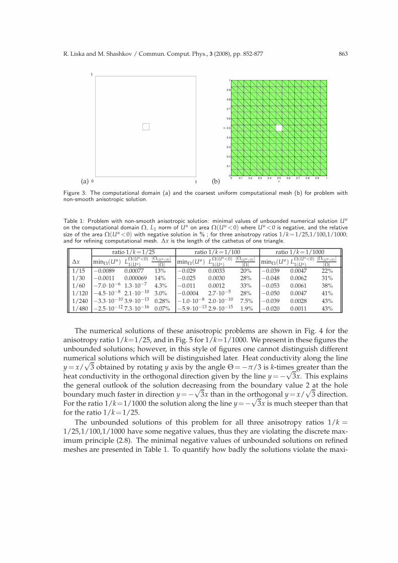
This problem originates in presentation [26], and its modified version has been used in[6]. The computational region is the unit square with a square hole with size 1/15×1/15(the hole is the square (7/15,8/15)2) in the center shown in Fig. 3(a).

We solve the homogeneous elliptic equation (2.1) with boundary conditions ψ=0 onthe outer boundary and ψ = 2 on the inner boundary along the hole. The anisotropicconductivity matrix A is created by the rotation of the diagonal matrix

B=

(

1 00 k

)

, (4.1)

where k is a parameter, by the orthogonal matrix R

R=

(

cosΘ −sinΘ

sinΘ cosΘ

)

(4.2)

with angle Θ=−π/3, so that

A=R·B·R′. (4.3)

We use three values of the parameter k, which defines anisotropy ratios 1/k of heat con-ductivity in two orthogonal directions, namely ratios 1/k=1/25,1/100 and 1/1000.

4.2.1 Uniform meshes

The computational region with the coarsest uniform triangular computational mesh isshown in Fig. 3(b). The triangles are rectangular with the length of their cathetus be-ing equal to ∆x=1/15. The finer computational meshes are created by uniform refiningof the mesh shown in Fig. 3(b) by splitting each triangle into four triangles with ver-tices at centers of edges of the original triangle. The meshes with the triangles catheti∆x=(1/15,1/30,1/60,1/120,1/240,1/480) have (448,1 792,7 168,28 672,114 688,458 752)triangles respectively.


(a) 0 1

1

(b)0 0.1 0.2 0.3 0.4 0.5 0.6 0.7 0.8 0.9 10

0.1

0.2

0.3

0.4

0.5

0.6

0.7

0.8

0.9

1

x

y

Figure 3: The computational domain (a) and the coarsest uniform computational mesh (b) for problem withnon-smooth anisotropic solution.

Table 1: Problem with non-smooth anisotropic solution: minimal values of unbounded numerical solution Uu

on the computational domain Ω, L1 norm of Uu on area Ω(Uu<0) where Uu

<0 is negative, and the relativesize of the area Ω(Uu

<0) with negative solution in % ; for three anisotropy ratios 1/k=1/25,1/100,1/1000;and for refining computational mesh. ∆x is the length of the cathetus of one triangle.

ratio 1/k=1/25 ratio 1/k=1/100 ratio 1/k=1/1000

∆x minΩ(Uu) LΩ(Uu

<0)1(Uu)

|Ω(Uu<0)||Ω| minΩ(Uu) L

Ω(Uu<0)

1(Uu)

|Ω(Uu<0)||Ω| minΩ(Uu) L

Ω(Uu<0)

1(Uu)

|Ω(Uu<0)||Ω|

1/15 −0.0089 0.00077 13% −0.029 0.0033 20% −0.039 0.0047 22%1/30 −0.0011 0.000069 14% −0.025 0.0030 28% −0.048 0.0062 31%1/60 −7.0·10−6 1.3·10−7 4.3% −0.011 0.0012 33% −0.053 0.0061 38%

1/120 −4.5·10−8 2.1·10−10 3.0% −0.0004 2.7·10−5 28% −0.050 0.0047 41%

1/240 −3.3·10−10 3.9·10−13 0.28% −1.0·10−8 2.0·10−10 7.5% −0.039 0.0028 43%

1/480 −2.5·10−12 7.3·10−16 0.07% −5.9·10−13 2.9·10−15 1.9% −0.020 0.0011 43%

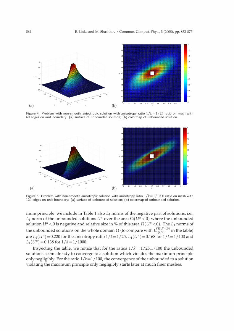
The numerical solutions of these anisotropic problems are shown in Fig. 4 for theanisotropy ratio 1/k=1/25, and in Fig. 5 for 1/k=1/1000. We present in these figures theunbounded solutions; however, in this style of figures one cannot distinguish differentnumerical solutions which will be distinguished later. Heat conductivity along the liney = x/

√3 obtained by rotating y axis by the angle Θ =−π/3 is k-times greater than the

heat conductivity in the orthogonal direction given by the line y=−√

3x. This explainsthe general outlook of the solution decreasing from the boundary value 2 at the holeboundary much faster in direction y=−

√3x than in the orthogonal y= x/

√3 direction.

For the ratio 1/k=1/1000 the solution along the line y=−√

3x is much steeper than thatfor the ratio 1/k=1/25.

The unbounded solutions of this problem for all three anisotropy ratios 1/k =1/25,1/100,1/1000 have some negative values, thus they are violating the discrete max-imum principle (2.8). The minimal negative values of unbounded solutions on refinedmeshes are presented in Table 1. To quantify how badly the solutions violate the maxi-


(a) 0

0.2

0.4

0.6

0.8

1

0

0.2

0.4

0.6

0.8

1

−0.5

0

0.5

1

1.5

2

xy

U

(b)0 0.1 0.2 0.3 0.4 0.5 0.6 0.7 0.8 0.9 10

0.1

0.2

0.3

0.4

0.5

0.6

0.7

0.8

0.9

1

x

y

0

0.2

0.4

0.6

0.8

1

1.2

1.4

1.6

1.8

2

Figure 4: Problem with non-smooth anisotropic solution with anisotropy ratio 1/k = 1/25 ratio on mesh with60 edges on unit boundary: (a) surface of unbounded solution; (b) colormap of unbounded solution.

(a) 0

0.2

0.4

0.6

0.8

1

0

0.2

0.4

0.6

0.8

1

−0.5

0

0.5

1

1.5

2

xy

U

(b)0 0.1 0.2 0.3 0.4 0.5 0.6 0.7 0.8 0.9 10

0.1

0.2

0.3

0.4

0.5

0.6

0.7

0.8

0.9

1

x

y

0

0.2

0.4

0.6

0.8

1

1.2

1.4

1.6

1.8

2

Figure 5: Problem with non-smooth anisotropic solution with anisotropy ratio 1/k=1/1000 ratio on mesh with120 edges on unit boundary: (a) surface of unbounded solution; (b) colormap of unbounded solution.

mum principle, we include in Table 1 also L1 norms of the negative part of solutions, i.e.,L1 norm of the unbounded solutions Uu over the area Ω(Uu

<0) where the unboundedsolution Uu

<0 is negative and relative size in % of this area Ω(Uu<0). The L1 norms of

the unbounded solutions on the whole domain Ω (to compare with LΩ(Uu

<0)1(Uu)

in the table)

are L1(Uu)=0.220 for the anisotropy ratio 1/k=1/25, L1(Uu)=0.168 for 1/k=1/100 andL1(Uu)=0.138 for 1/k=1/1000.

Inspecting the table, we notice that for the ratios 1/k = 1/25,1/100 the unboundedsolutions seem already to converge to a solution which violates the maximum principleonly negligibly. For the ratio 1/k=1/100, the convergence of the unbounded to a solutionviolating the maximum principle only negligibly starts later at much finer meshes.


Table 2: Problem with non-smooth anisotropic solution: convergence for the anisotropy ratio 1/k = 1/25: L1norm of error (difference from the reference unbounded solution on mesh with ∆x = 1/480) and ratios of twosuccessive error norms for the unbounded, bounded, constrained-bounded and repaired solutions.

unbounded bounded constrained- repairedbounded

∆x Lerr1 ratio Lerr

1 ratio Lerr1 ratio Lerr

1 ratio

1/15 0.0925 1.95 0.0921 1.95 0.0909 1.93 0.0914 1.931/30 0.0474 2.20 0.0473 2.20 0.0472 2.20 0.0474 2.301/60 0.0215 2.40 0.0215 2.40 0.0215 2.40 0.0215 2.40

1/120 0.0090 0.0090 0.0090 0.0090

Table 3: Problem with non-smooth anisotropic solution: convergence for the anisotropy ratio 1/k=1/100: L1norm of error (difference from the reference unbounded solution on mesh with ∆x = 1/480) and ratios of twosuccessive error norms for the unbounded, bounded, constrained-bounded and repaired solutions.

unbounded bounded constrained- repairedbounded

∆x Lerr1 ratio Lerr

1 ratio Lerr1 ratio Lerr

1 ratio

1/15 0.1428 1.66 0.1419 1.68 0.1374 1.71 0.1363 1.701/30 0.0858 1.96 0.0844 1.98 0.0804 1.95 0.0804 1.891/60 0.0437 2.35 0.0427 2.30 0.0412 2.23 0.0426 2.29

1/120 0.0186 0.0185 0.0185 0.0186

The exact solution for this problem is not known, so for the convergence study we usethe reference unbounded solution computed on the finest mesh with triangles cathetus∆x = 1/480. The convergence for the unbounded, bounded, constrained-bounded, andrepaired solutions for meshes with ∆x = 1/15,1/30,1/60,1/120 is presented in Table 2for the anisotropy ratio 1/k=1/25 and in Table 3 for 1/k=1/100. The unbounded solu-tions providing the same results as standard linear FEM is known to converge from the-ory [19], and the convergence tables also show that the bounded, constrained-boundedand repaired solutions do converge. So the imposed constraints do not destroy the con-vergence. As the solution is non-smooth, the convergence is only first order. Strictlyspeaking of course the solution of the elliptic problem is smooth; by non-smooth we meanhere that the gradient of the solution in the low conductivity direction changes very fastfrom very steep to flat. We have not made the convergence study for the anisotropy ratio1/k=1/1000, as the unbounded solution on our finest mesh has still rather large error ofthe order 1% (the relative L1 norm of negative part of the solution), see Table 1.

To understand the difference in behavior of the solutions for two different ratios 1/k,we present in Fig. 6 the areas where the unbounded solutions are negative for ratio 1/k=1/25, and the same in Fig. 7 for ratio 1/k=1/1000. In both cases for the first four refinedmeshes with the triangles cathetus ∆x=1/15,1/30,1/60,1/120. The areas with a negativesolution are presented by colormaps showing only negative values by different colors


(a)0 0.1 0.2 0.3 0.4 0.5 0.6 0.7 0.8 0.9 1

0

0.1

0.2

0.3

0.4

0.5

0.6

0.7

0.8

0.9

1 unbounded

x

y

−8

−7

−6

−5

−4

−3

−2

−1

0x 10

−3

(b)0 0.1 0.2 0.3 0.4 0.5 0.6 0.7 0.8 0.9 1

0

0.1

0.2

0.3

0.4

0.5

0.6

0.7

0.8

0.9

1 unbounded

x

y

−10

−8

−6

−4

−2

0x 10

−4

(c)0 0.1 0.2 0.3 0.4 0.5 0.6 0.7 0.8 0.9 1

0

0.1

0.2

0.3

0.4

0.5

0.6

0.7

0.8

0.9

1 unbounded

x

y

−6

−5

−4

−3

−2

−1

0x 10

−6

(d)0 0.1 0.2 0.3 0.4 0.5 0.6 0.7 0.8 0.9 1

0

0.1

0.2

0.3

0.4

0.5

0.6

0.7

0.8

0.9

1 unbounded

x

y

−4.5

−4

−3.5

−3

−2.5

−2

−1.5

−1

−0.5

0x 10

−8

Figure 6: Problem with non-smooth anisotropic solution with anisotropy ratio 1/k = 1/25, colormaps of un-bounded solution showing areas where the solution is negative (areas where the solution is non-negative arewhite) on: (a) mesh with 15 edges on unit boundary; (b) mesh with 30 edges on unit boundary; (c) mesh with60 edges on unit boundary; (d) mesh with 120 edges on unit boundary.

and with all positive values presented in white. In Fig. 6 the lower end of the interval forthe colormap is given by the minimal negative value presented in Table 1, and the upperend of the interval is zero. The minimal values are increasing towards zero with meshrefinement, and the area where the unbounded solution is negative is getting smallerwith refinement. On the other hand, the color map interval for all refinement levels inFig. 7 for ratio 1/k = 1/1000 remains (-0.05,0) the regions of negative solutions movetowards the solution ridge with refinement creating oscillations. However, the areas ofthese regions are not getting smaller. It seems that we would need much higher resolutionfor the unbounded solution to violate less the maximum principle.

To see the differences between different numerical solutions, we have chosen topresent 1D cuts of the solutions along the line y = 7/15, which is the line defining thelower boundary of the square hole in the solution domain. The 1D cuts are presented forthe ratio 1/k =1/1000 for which the differences are more visible. Fig. 8 (a),(b) compares


(a)0 0.1 0.2 0.3 0.4 0.5 0.6 0.7 0.8 0.9 1

0

0.1

0.2

0.3

0.4

0.5

0.6

0.7

0.8

0.9

1 unbounded

x

y

−0.035

−0.03

−0.025

−0.02

−0.015

−0.01

−0.005

0

(b)0 0.1 0.2 0.3 0.4 0.5 0.6 0.7 0.8 0.9 1

0

0.1

0.2

0.3

0.4

0.5

0.6

0.7

0.8

0.9

1 unbounded

x

y

−0.045

−0.04

−0.035

−0.03

−0.025

−0.02

−0.015

−0.01

−0.005

0

(c)0 0.1 0.2 0.3 0.4 0.5 0.6 0.7 0.8 0.9 1

0

0.1

0.2

0.3

0.4

0.5

0.6

0.7

0.8

0.9

1 unbounded

x

y

−0.05

−0.045

−0.04

−0.035

−0.03

−0.025

−0.02

−0.015

−0.01

−0.005

0

(d)0 0.1 0.2 0.3 0.4 0.5 0.6 0.7 0.8 0.9 1

0

0.1

0.2

0.3

0.4

0.5

0.6

0.7

0.8

0.9

1 unbounded

x

y

−0.045

−0.04

−0.035

−0.03

−0.025

−0.02

−0.015

−0.01

−0.005

0

Figure 7: Problem with non-smooth anisotropic solution with anisotropy ratio 1/k = 1/1000, colormaps ofunbounded solution showing areas where the solution is negative (areas where the solution is non-negative arewhite) on: (a) mesh with 15 edges on unit boundary; (b) mesh with 30 edges on unit boundary; (c) mesh with60 edges on unit boundary; (d) mesh with 120 edges on unit boundary.

1D cuts of unbounded, bounded, constrained-bounded, and repaired solutions on thefinest mesh with 120 cell edges on the outer unit boundary. The unbounded solution isnegative in some regions of x. The repaired solution is not smooth with a jump in its gra-dient which is clearly bad as the solution of the Laplace equation should have a smoothgradient. The best seem to be the bounded and constrained-bounded solutions which arequite close to each other. They are smooth and positive, i.e., satisfy the maximum princi-ple. To show the oscillations (from the positive to negative values) of the solution alongthe diagonal y=1−x visible in the solution on the finest mesh in Fig. 7(d), in Fig. 8(c) wepresent the 1D cut of this solution on the finest mesh with 120 edges on unit boundary.In Fig. 8(c) the green line presents the unbounded solution Uu plotted in the standardlinear scale and the blue line presents absolute value |Uu| of the unbounded solution inthe logarithmic scale. Each sharp local minimum on this logarithmic plot corresponds toone change of the sign of Uu where its value passes through zero and the absolute value


(a) 0 0.1 0.2 0.3 0.4 0.5 0.6 0.7 0.8 0.9 1−0.5

0

0.5

1

1.5

2

x

U

unbounded

bounded

constrained bounded

repaired

(b) 0 0.1 0.2 0.3 0.4 0.5 0.6 0.7 0.8 0.9 1−0.05

0

0.05

0.1

x

U

unbounded

bounded

constrained bounded

repaired

(c) 0 0.1 0.2 0.3 0.4 0.5 0.6 0.7 0.8 0.9 110

−10

10−8

10−6

10−4

10−2

100

x

U

0 0.1 0.2 0.3 0.4 0.5 0.6 0.7 0.8 0.9 110

−10

10−8

10−6

10−4

10−2

100

x

U

0 0.1 0.2 0.3 0.4 0.5 0.6 0.7 0.8 0.9 1

100

x

U

0 0.1 0.2 0.3 0.4 0.5 0.6 0.7 0.8 0.9 1−0.05

−0.04

−0.03

−0.02

−0.01

0

0.01

U

Figure 8: Problem with non-smooth anisotropic solution with the anisotropy ratio 1/k = 1/1000 on the meshwith 120 edges on unit boundary: (a) full view and (b) view zoomed, scaled in y direction of 1D cuts alongthe line y=7/15, comparison of unbounded, bounded, constrained-bounded and repaired solution; (c) 1D cutof unbounded solution Uu along the diagonal y=1−x, green is Uu with the right linear axis and blue is |Uu|with the left logarithmic axis.


(a)0 0.1 0.2 0.3 0.4 0.5 0.6 0.7 0.8 0.9 1

−0.5

0

0.5

1

1.5

2

x

U15 cells

30 cells

60 cells

120 cells

(b)0 0.1 0.2 0.3 0.4 0.5 0.6 0.7 0.8 0.9 1

−0.05

0

0.05

0.1

x

U

15 cells30 cells60 cells120 cells

(c)0 0.1 0.2 0.3 0.4 0.5 0.6 0.7 0.8 0.9 1

0

0.2

0.4

0.6

0.8

1

1.2

1.4

1.6

1.8

2

x

U

15 cells

30 cells

60 cells

120 cells

(d)0 0.1 0.2 0.3 0.4 0.5 0.6 0.7 0.8 0.9 1

0

0.2

0.4

0.6

0.8

1

1.2

1.4

1.6

1.8

2

x

U

15 cells

30 cells

60 cells

120 cells

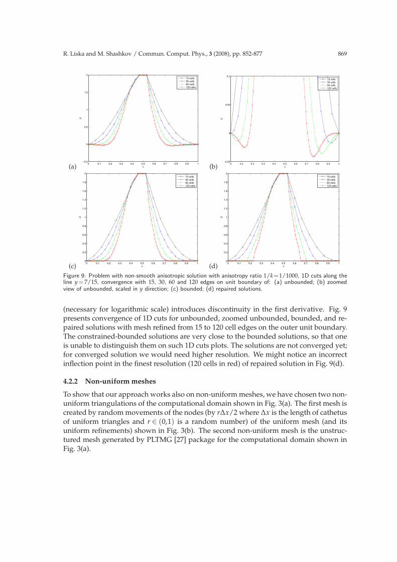
Figure 9: Problem with non-smooth anisotropic solution with anisotropy ratio 1/k=1/1000, 1D cuts along theline y = 7/15, convergence with 15, 30, 60 and 120 edges on unit boundary of: (a) unbounded; (b) zoomedview of unbounded, scaled in y direction; (c) bounded; (d) repaired solutions.

(necessary for logarithmic scale) introduces discontinuity in the first derivative. Fig. 9presents convergence of 1D cuts for unbounded, zoomed unbounded, bounded, and re-paired solutions with mesh refined from 15 to 120 cell edges on the outer unit boundary.The constrained-bounded solutions are very close to the bounded solutions, so that oneis unable to distinguish them on such 1D cuts plots. The solutions are not converged yet;for converged solution we would need higher resolution. We might notice an incorrectinflection point in the finest resolution (120 cells in red) of repaired solution in Fig. 9(d).

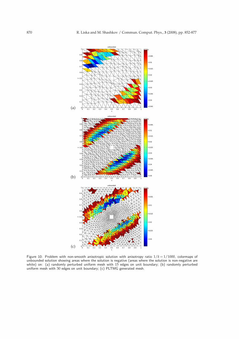
4.2.2 Non-uniform meshes

To show that our approach works also on non-uniform meshes, we have chosen two non-uniform triangulations of the computational domain shown in Fig. 3(a). The first mesh iscreated by random movements of the nodes (by r∆x/2 where ∆x is the length of cathetusof uniform triangles and r ∈ (0,1) is a random number) of the uniform mesh (and itsuniform refinements) shown in Fig. 3(b). The second non-uniform mesh is the unstruc-tured mesh generated by PLTMG [27] package for the computational domain shown inFig. 3(a).


(a) 0 0.1 0.2 0.3 0.4 0.5 0.6 0.7 0.8 0.9 10

0.1

0.2

0.3

0.4

0.5

0.6

0.7

0.8

0.9

1 unbounded

x

y

−0.045

−0.04

−0.035

−0.03

−0.025

−0.02

−0.015

−0.01

−0.005

0

(b) 0 0.1 0.2 0.3 0.4 0.5 0.6 0.7 0.8 0.9 10

0.1

0.2

0.3

0.4

0.5

0.6

0.7

0.8

0.9

1 unbounded

x

y

−0.05

−0.045

−0.04

−0.035

−0.03

−0.025

−0.02

−0.015

−0.01

−0.005

0

(c) 0 0.1 0.2 0.3 0.4 0.5 0.6 0.7 0.8 0.9 10

0.1

0.2

0.3

0.4

0.5

0.6

0.7

0.8

0.9

1 unbounded

x

y

−0.03

−0.025

−0.02

−0.015

−0.01

−0.005

0

Figure 10: Problem with non-smooth anisotropic solution with anisotropy ratio 1/k = 1/1000, colormaps ofunbounded solution showing areas where the solution is negative (areas where the solution is non-negative arewhite) on: (a) randomly perturbed uniform mesh with 15 edges on unit boundary; (b) randomly perturbeduniform mesh with 30 edges on unit boundary; (c) PLTMG generated mesh.


Table 4: Problem with non-smooth anisotropic solution with anisotropy ratio 1/k = 1/100 on unstructuredmeshes: minimal values of unbounded numerical solution Uu on the computational domain Ω, L1 norm of Uu

on area Ω(Uu<0) where Uu

<0 is negative, and the relative size of the area Ω(Uu<0) with negative solution

in % ; for refining computational meshes. The L1 norm of the unbounded reference solution (with ∆x=1/480)

on the whole domain Ω on the uniform mesh (to compare with LΩ(Uu

<0)1(Uu)

in the table) is L1(Uu)=0.168.

Nr. of triangles minΩ(Uu) LΩ(Uu

<0)1(Uu)

|Ω(Uu<0)||Ω|

112 −0.001 2.1·10−5 5.9 %448 −0.011 3.8·10−4 27 %

1792 −0.0033 2.3·10−4 31 %7168 −0.0003 1.1·10−5 25 %

28672 −1.8·10−6 2.1·10−8 7.1 %

Again, the unbounded solutions on such meshes violate the maximum principlewhile the bounded, constrained-bounded, and repaired do not violate the maximumprinciple. The general shape of solution remains the same and corresponds approxi-mately (depending on mesh resolution) to that for the uniform mesh presented in Figs. 4and 5. We present here only the colormaps of areas with negative solution (violating themaximum principle) for two randomly perturbed uniform meshes and for one unstruc-tured PLTMG mesh in Fig. 10 for the anisotropy ratio k=1/1000.

The minimal negative values of unbounded solutions on refined unstructured meshesfor the anisotropy ratio 1/k=1/100 are presented in Table 4. To quantify how badly thesolutions violate the maximum principle, we included in Table 4 also L1 norms of neg-ative part of solutions, i.e., L1 norm of unbounded solutions Uu over area Ω(Uu

< 0)where Uu

< 0 is negative and relative size in % of the area Ω(Uu< 0) where the so-

lution is negative. As the unstructured meshes have more smaller triangles aroundthe central hole, the unbounded solutions on these meshes violate the maximum prin-ciple less than that on uniform meshes with the same number of triangles, comparewith Table 1 for uniform triangulations, where the meshes with uniform triangle catheti∆x=(1/15,1/30,1/60,1/120) have (448, 1 792, 7 168, 28 672) triangles, respectively.

5 Numerical experiments for non-homogeneous equation

In this section we will present several numerical tests solving the Poisson equation (2.1)with non-negative sources f ≥ 0 and zero Dirichlet boundary conditions ψ = 0. Themaximum principle for f ≥ 0 (2.5) and ψ = 0 implies that the solution has to be non-negative u≥0 everywhere. The presented tests violate this maximum principle for the un-bounded solution which is exactly the same as the standard linear finite element solution.Below, we present only numerical results of the unbounded solutions. The bounded,constrained-bounded, and repaired solutions for all the presented problems satisfy thediscrete maximum principle (2.8), i.e., are non-negative everywhere.


5.1 Simple isotropic problem

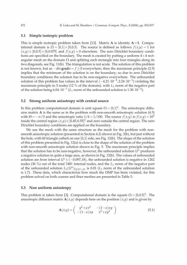
This is simple isotropic problem taken from [13]. Matrix A is identity A= I. Compu-tational domain is Ω = [0,1]×[0,0.3]. The source is defined as follows f (x,y) = 1 for(x,y)∈ [0,0.5]×[0,0.075] and f (x,y) = 0 elsewhere. The zero Dirichlet boundary condi-tions are specified on the boundary. The mesh is created by putting a uniform 4×4 rect-angular mesh on the domain Ω and splitting each rectangle into four triangles along itstwo diagonals, see Fig. 11(b). The triangulation is not acute. The solution of this problemis not known, but as −divgradu = f ≥ 0 everywhere, then the maximum principle (2.5)implies that the minimum of the solution is on the boundary; so due to zero Dirichletboundary conditions the solution has to be non-negative everywhere. The unboundedsolution of this problem has values in the interval (−4.21·10−5, 2.24·10−3) violating themaximum principle in 3 nodes (12 % of the domain), with L1 norm of the negative partof the solution being 6.04·10−7 (L1 norm of the unbounded solution is 1.30·10−4).

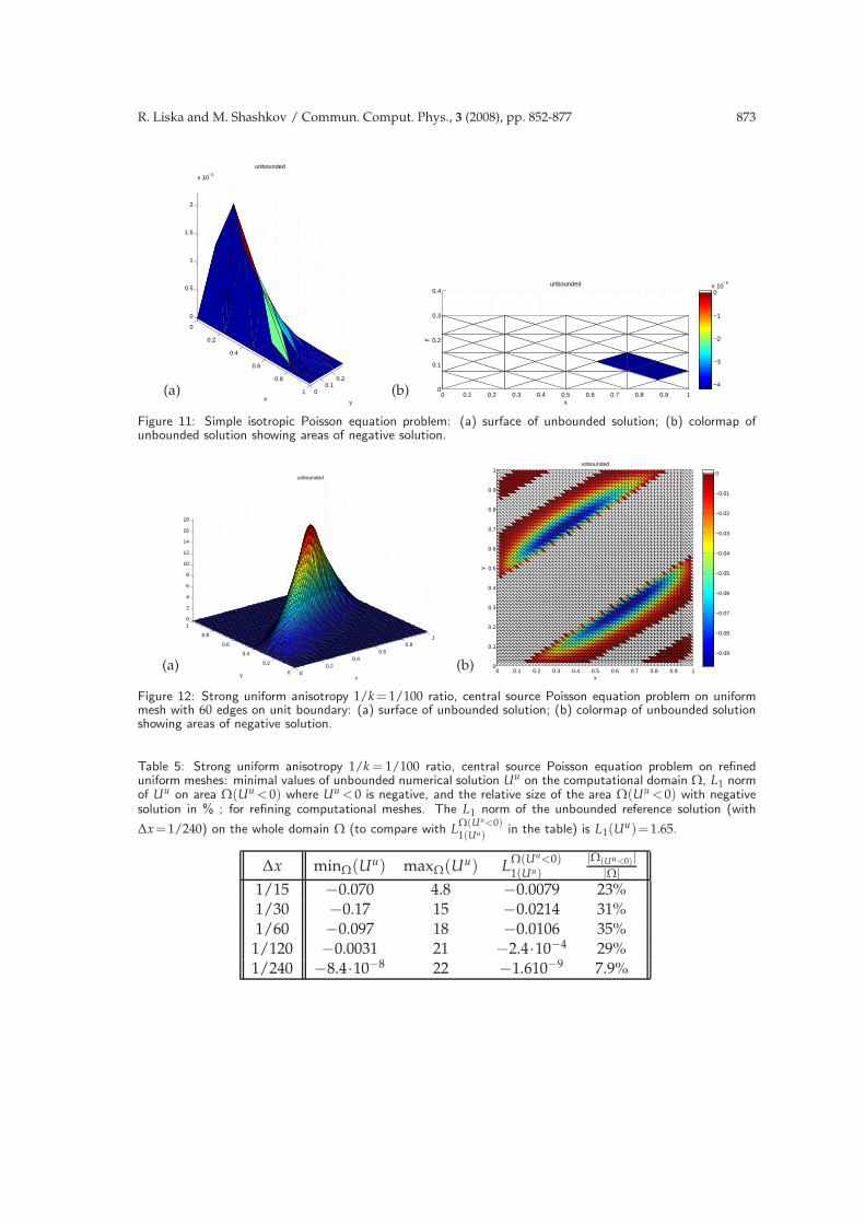
5.2 Strong uniform anisotropy with central source

In this problem computational domain is unit square Ω = [0,1]2. The anisotropic diffu-sion matrix A is the same as in the problem with non-smooth anisotropic solution (4.3)with Θ=−π/3 and the anisotropic ratio 1/k =1/100. The source f (x,y) is f (x,y)=105

inside the central region (x,y)∈ [0.45,0.55]2 and zero outside the central region. The zeroDirichlet boundary conditions are applied on the boundary.

We use the mesh with the same structure as the mesh for the problem with non-smooth anisotropic solution (presented in Section 4.2) shown in Fig. 3(b), but just withoutthe hole, with 60 triangle catheti on one [0,1] side, see Fig. 12(b). The shape of the solutionof this problem presented in Fig. 12(a) is close to the shape of the solution of the problemwith non-smooth anisotropic solution shown in Fig. 5. The maximum principle impliesthat the solution has to be non-negative, however, the unbounded solution Uu producesa negative solution in quite a large area, as shown in Fig. 12(b). The values of unboundedsolution are from interval Uu ∈ (−0.097,18), the unbounded solution is negative in 1262nodes (36 %) out of the total 3481 internal nodes, and the L1 norm of the negative partof the unbounded solution L1(Uu)Ω(Uu<0) is 0.01 (L1 norm of the unbounded solutionis 1.7). These data, which characterize how much the DMP has been violated, for thisproblem solved on both coarser and finer meshes are presented in Table 5.

5.3 Non uniform anisotropy

This problem is taken from [3]. Computational domain is the square Ω = [0,0.5]2. Theanisotropic diffusion matrix A(x,y) depends here on the position (x,y) and is given by

A(x,y)=

(

y2+ǫx2 −(1−ǫ)xy−(1−ǫ)xy x2+ǫy2

)

(5.1)


(a)

0

0.2

0.4

0.6

0.8

1 00.1

0.2

0

0.5

1

1.5

2

x 10−3

y

unbounded

x(b) 0 0.1 0.2 0.3 0.4 0.5 0.6 0.7 0.8 0.9 1

0

0.1

0.2

0.3

0.4 unbounded

x

y

−4

−3

−2

−1

0x 10

−5

Figure 11: Simple isotropic Poisson equation problem: (a) surface of unbounded solution; (b) colormap ofunbounded solution showing areas of negative solution.

(a)0

0.20.4

0.60.8

1

0

0.2

0.4

0.6

0.8

10

2

4

6

8

10

12

14

16

18

x

unbounded

y(b) 0 0.1 0.2 0.3 0.4 0.5 0.6 0.7 0.8 0.9 1

0

0.1

0.2

0.3

0.4

0.5

0.6

0.7

0.8

0.9

1 unbounded

x

y

−0.09

−0.08

−0.07

−0.06

−0.05

−0.04

−0.03

−0.02

−0.01

0

Figure 12: Strong uniform anisotropy 1/k = 1/100 ratio, central source Poisson equation problem on uniformmesh with 60 edges on unit boundary: (a) surface of unbounded solution; (b) colormap of unbounded solutionshowing areas of negative solution.

Table 5: Strong uniform anisotropy 1/k = 1/100 ratio, central source Poisson equation problem on refineduniform meshes: minimal values of unbounded numerical solution Uu on the computational domain Ω, L1 normof Uu on area Ω(Uu

<0) where Uu<0 is negative, and the relative size of the area Ω(Uu

<0) with negativesolution in % ; for refining computational meshes. The L1 norm of the unbounded reference solution (with

∆x=1/240) on the whole domain Ω (to compare with LΩ(Uu

<0)1(Uu)

in the table) is L1(Uu)=1.65.

∆x minΩ(Uu) maxΩ(Uu) LΩ(Uu

<0)1(Uu)

|Ω(Uu<0)||Ω|

1/15 −0.070 4.8 −0.0079 23%1/30 −0.17 15 −0.0214 31%1/60 −0.097 18 −0.0106 35%

1/120 −0.0031 21 −2.4·10−4 29%1/240 −8.4·10−8 22 −1.610−9 7.9%


with ǫ=10−3 which gives the anisotropy ratio. The source f (x,y) is f (x,y)=1 for (x,y)∈[0.125,0.375]2 and zero otherwise. The zero Dirichlet boundary conditions are applied onthe boundary.

For this problem we use the triangular mesh obtained from the uniform orthogonalmesh of 30×30 squares by splitting each square cell into four triangles by two diagonalsof the square, see Fig. 13(b). The surface plot of the unbound solution to this problemis shown in Fig. 13(a). The maximum principle (2.5) implies that the solution has to benon-negative, however the unbounded solution Uu produces a negative solution in quitea large area, as shown in Fig. 13(b). The values of unbounded solution are from intervalUu ∈ (−2.010−3,0.26), the unbounded solution is negative in 209 nodes (12 %) out of thetotal 1741 internal nodes, and the L1 norm of the negative part of the unbounded solutionL1(Uu)Ω(Uu<0) is 8.1·10−6 (L1 norm of the unbounded solution is 0.019).

5.4 Non uniform rotating anisotropy

For this problem computational domain is unit square Ω = [0,1]2. The anisotropic dif-fusion matrix A(x,y) depends on the position (x,y) and is given by the rotation of thediagonal matrix (4.1) around the origin by the angle ϕ which is the angular polar coordi-nate of the point (x,y):

A(x,y)=

(

cosϕ −sinϕsinϕ cosϕ

)

·(

1 00 k

)

·(

cos ϕ sinϕ−sinϕ cos ϕ

)

(5.2)

with k=1000 which gives the anisotropy ratio and

cosϕ= x/r, sinϕ=y/r, r=√

x2+y2.

The source f (x,y) is f (x,y) = 105 for (x,y)∈ (0.7,0.8)×(0,0.1) and zero elsewhere. Thezero Dirichlet boundary conditions are applied on the boundary.

For this problem we use the triangular mesh obtained from the uniform orthogonalmesh of 20×20 squares by splitting each square cell into four triangles by two diagonalsof the square, see Fig. 14(b). The surface plot of the unbounded solution to this problemis shown in Fig. 14(a). The maximum principle implies that the solution has to be non-negative, however, the unbounded solution Uu produces a negative solution in quite alarge area, as shown in Fig. 14(b). The values of unbounded solution are from intervalUu ∈ (−0.015,0.47), the unbounded solution is negative in 354 nodes (46 %) out of thetotal 761 internal nodes, and the L1 norm of the negative part of the unbounded solutionL1(Uu)Ω(Uu<0) is 1.310−3 (L1 norm of the unbounded solution is 0.031).

6 Conclusion

We have proposed two new methods for enforcing discrete maximum principle for linearfinite element solutions on 2D triangular mesh of the linear second-order self-adjoint


(a)

00.1

0.20.3

0.40.5 0

0.10.2

0.30.4

0.50

0.05

0.1

0.15

0.2

0.25

y

unbounded

x

(b) 0 0.05 0.1 0.15 0.2 0.25 0.3 0.35 0.4 0.45 0.50

0.05

0.1

0.15

0.2

0.25

0.3

0.35

0.4

0.45

0.5 unbounded

x

y

−2

−1.8

−1.6

−1.4

−1.2

−1

−0.8

−0.6

−0.4

−0.2

0x 10

−3

Figure 13: Non uniform anisotropy Poisson equation problem: (a) surface of unbounded solution; (b) colormapof unbounded solution showing areas of negative solution.

(a)

0

0.2

0.4

0.6

0.8

1 00.1

0.20.3

0.40.5

0.60.7

0.80.9

1

0

0.1

0.2

0.3

0.4

y

unbounded

x

(b) 0 0.1 0.2 0.3 0.4 0.5 0.6 0.7 0.8 0.9 10

0.1

0.2

0.3

0.4

0.5

0.6

0.7

0.8

0.9

1 unbounded

x

y

−15

−10

−5

0x 10

−3

Figure 14: Non uniform rotating anisotropy Poisson equation problem on uniform mesh: (a) surface of un-bounded solution; (b) colormap of unbounded solution showing areas of negative solution.

elliptic equation without lower-order terms.

First approach is based on repair technique, which is a posteriori correction of thediscrete solution. Second method is based on constrained optimization.

Numerical experiments demonstrate the ability of the new methods to produce nu-merical solutions satisfying the discrete maximum principle, contrary to the standardlinear finite element method.

Numerical experiments also show that convergence rate of new methods is about thesame as for original linear finite element method.

In the future we plan to analyze method using constrained optimization with respectto its performance. We hope that we will be able to develop more practical method takinginto account that we are solving very special quadratic optimization problem with verysimple constraints. We also planning to extend optimization method to the case of mixedfinite element [29] and mimetic discretizations [28].


Acknowledgments

This work was carried out under the auspices of the National Nuclear Security Adminis-tration of the U.S. Department of Energy at Los Alamos National Laboratory under Con-tract No. DE-AC52-06NA25396 and the DOE Office of Science Advanced Scientific Com-puting Research (ASCR) Program in Applied Mathematics Research. The first author hasbeen supported in part by the Czech Ministry of Education projects MSM 6840770022 andLC06052 (Necas Center for Mathematical Modeling). We thank M. Berndt, K. Lipnikovand D. Svyatskiy for fruitful discussion.

References

[1] A. Draganescu, T. F. Dupont and L. R. Scott, Failure of the discrete maximum principle foran elliptic finite element problem, Math. Comput., 74(249) (2005), 1-23.

[2] C. Le Potier, Finite volume scheme for highly anisotropic diffusion operators on unstruc-tured meshes, CR Acad. Sci. I–Math., 340(12) (2005), 921-926.

[3] C. Le Potier, Finite volume monotone scheme for highly anisotropic diffusion operators onunstructured triangular meshes, CR Acad. Sci. I–Math., 341(12) (2005), 787-792, 2005.

[4] J. Droniou and R. Eymard, A mixed finite volume scheme for anisotropic diffusion problemson any grid, Numer. Math., 105(1) (2006), 35-71.

[5] M. J. Mlacnik and L. J. Durlofsky, Unstructured grid optimization for improved monotonic-ity of discrete solutions of elliptic equations with highly anisotropic coefficients, J. Comput.Phys., 216(1) (2006), 337-361.

[6] K. Lipnikov, M. Shashkov, D. Svyatskiy and Y. Vassilevski, Monotone finite volume schemesfor diffusion equations on unstructured triangular and shape-regular polygonal meshes, J.Comput. Phys., 227(1) (2007), 492-512.

[7] J. M. Nordbotten, I. Aavatsmark and G. T. Eigestad, Monotonicity of control volume meth-ods, Numer. Math., 106(2) (2007), 255-288.

[8] P. G. Ciarlet and P. A. Raviart, Maximum principle and uniform convergence for the finiteelement method, Comput. Method. Appl. Mech. Engrg., 2(1) (1973), 17-31.

[9] M. Krizek and L. Liu, Finite element approximation of a nonlinear heat conduction problemin anisotropic media, Comput. Method. Appl. Mech. Engrg., 157(3-4) (1998), 387-397.

[10] M. Krizek and L. P. Liu, On the maximum and comparison principles for a steady-statenonlinear heat conduction problem, Z. Angew. Math. Mech., 83(8) (2003), 559-563.

[11] J. Karatson and S. Korotov, Discrete maximum principles for finite element solutions ofnonlinear elliptic problems with mixed boundary conditions, Numer. Math., 99(4) (2005),669-698.

[12] J. Karatson and S. Korotov, Discrete maximum principles for finite element solutions ofsome mixed nonlinear elliptic problems using quadratures, J. Comput. Appl. Math., 192(1)(2006), 75-88.

[13] E. Burman and A. Ern, Discrete maximum principle for galerkin approximations of thelaplace operator on arbitrary meshes, CR Acad. Sci. I–Math., 338(8) (2004), 641-646.

[14] T. Vejchodsky and P. Solin, Discrete maximum principle for a problem with piecewise-constant coefficients solved by hp-fem, Technical Report 2006-10, University of Texas at ElPaso, Dept. of Mathematical Sciences, 2006.


[15] S. Deng, K. Ito and Z. Li, Three-dimensional elliptic solvers for interface problems andapplications, J. Comput. Phys., 184(1) (2003), 215-243.

[16] H. Hoteit, R. Mose, B. Philippe, P. Ackerer and J. Erhel, The maximum principle violationsof the mixed-hybrid finite-element method applied to diffusion equations, Int. J. Numer.Meth. Eng., 55(12) (2002), 1373-1390.

[17] J. C. Strikwerda, Finite Difference Schemes and Partial Differential Equations, Wadsworth,Inc., Belmont, 1989.

[18] M. Shashkov, Conservative Finite-Difference Methods on General Grids, CRC Press, BocaRaton, Florida, 1996.

[19] P. G. Ciarlet, Basic error estimates for elliptic problems, in: P. G. Ciarlet and J. L. Lions(Eds.), Handbook of Numerical Analysis, Volume II: Finite Element Methods (Part 1), Else-vier, 1990.

[20] M. Kucharık, M. Shashkov and B. Wendroff, An efficient linearity-and-bound-preservingremapping method, J. Comput. Phys., 188(2) (2003), 462-471.

[21] M. Shashkov and B. Wendroff, The repair paradigm and application to conservation laws,J. Comput. Phys., 198(1) (2004), 265-277.

[22] R. L. Loubere, M. Staley and B. Wendroff, The repair paradigm: New algorithms and appli-cations to compressible flow, J. Comput. Phys., 211(2) (2006), 385-404.

[23] K. Schittkowski, QL: A Fortran code for convex quadratic programming – user’s guide,Technical Report, University of Bayreuth, 2003.

[24] M. J. D. Powell, On the quadratic programming algorithm of Goldfarb and Idnani, TechnicalReport DAMTP 1983/Na 19, University of Cambridge, Cambridge, 1983.

[25] D. Goldfarb and A. Idnani, A numerically stable method for solving strictly convexquadratic programs, Math. Program., 27 (1983), 1-33.

[26] M. Mlacnik, L. Durlofsky, R. Juanes and H. Tchelepi, Multipoint flux approximations forreservoir simulation, 12th Annual SUPRI-HW Meeting, November 18-19, Stanford Univer-sity, 2004.

[27] R. E. Bank, PLTMG: A Software Package for Solving Elliptic Partial Differential Equations.Users’ Guide 8.0, SIAM Publisher, Philadelphia, 1998.

[28] J. Hyman, M. Shashkov and S. Steinberg, The numerical solution of diffusion problems instrongly heterogeneous non-isotropic materials, J. Comput. Phys., 132 (1997), 130-148.

[29] F. Brezzi and M. Fortin, Mixed and Hybrid Finite Element Methods, Springer-Verlag, NewYork, 1991.

Date post:	30-Aug-2018
Category:	Documents
Upload:	buituyen
View:	214 times
Download:	0 times

Enforcing the Discrete Maximum Principle for Linear Finite...

Documents