Engineering a Scalable Placement Heuristic for DNA Probe Arrays A.B. Kahng, I.I. Mandoiu, P. A.B. Kahng, I.I. Mandoiu, P. Pevzner, Pevzner, S. Reda (all UCSD), A. S. Reda (all UCSD), A. Zelikovsky (GSU) Zelikovsky (GSU)
Transcript
Engineering a Scalable Placement Heuristic for DNA
Probe Arrays
A.B. Kahng, I.I. Mandoiu, P. Pevzner, A.B. Kahng, I.I. Mandoiu, P. Pevzner,
S. Reda (all UCSD), A. Zelikovsky (GSU)S. Reda (all UCSD), A. Zelikovsky (GSU)
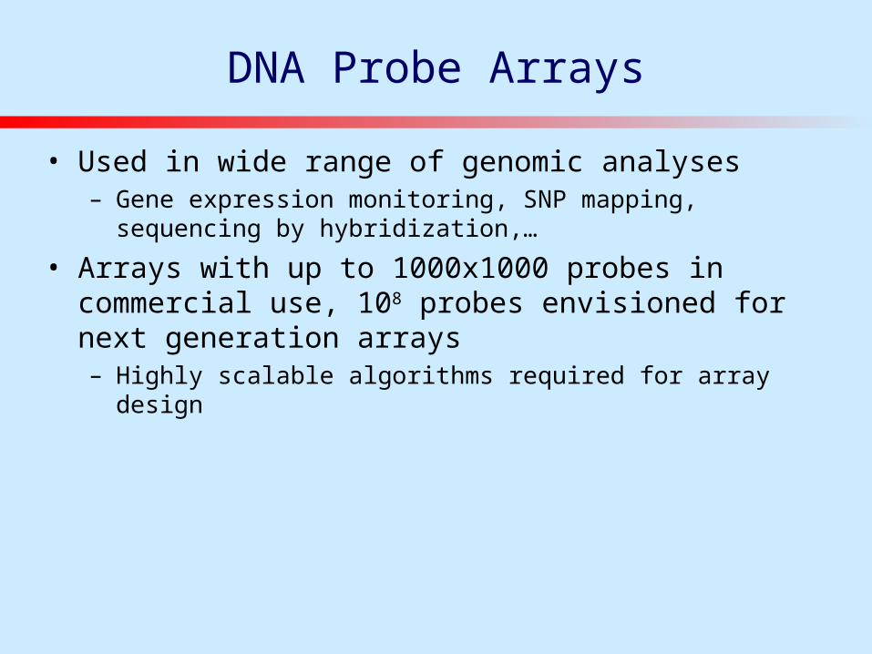
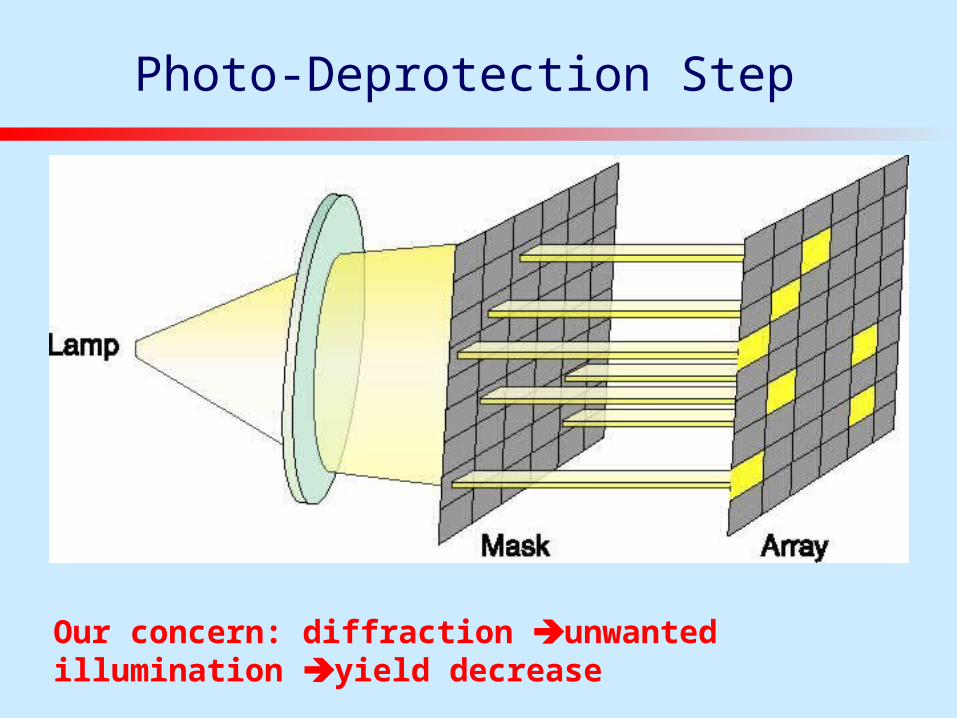
• Used in wide range of genomic analyses– Gene expression monitoring, SNP mapping, sequencing by
hybridization,…
• Arrays with up to 1000x1000 probes in commercial use, 108 probes envisioned for next generation arrays– Highly scalable algorithms required for array design
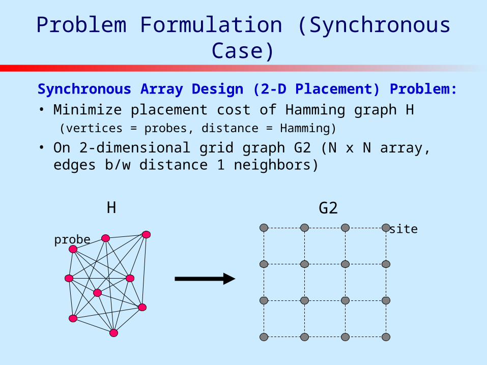
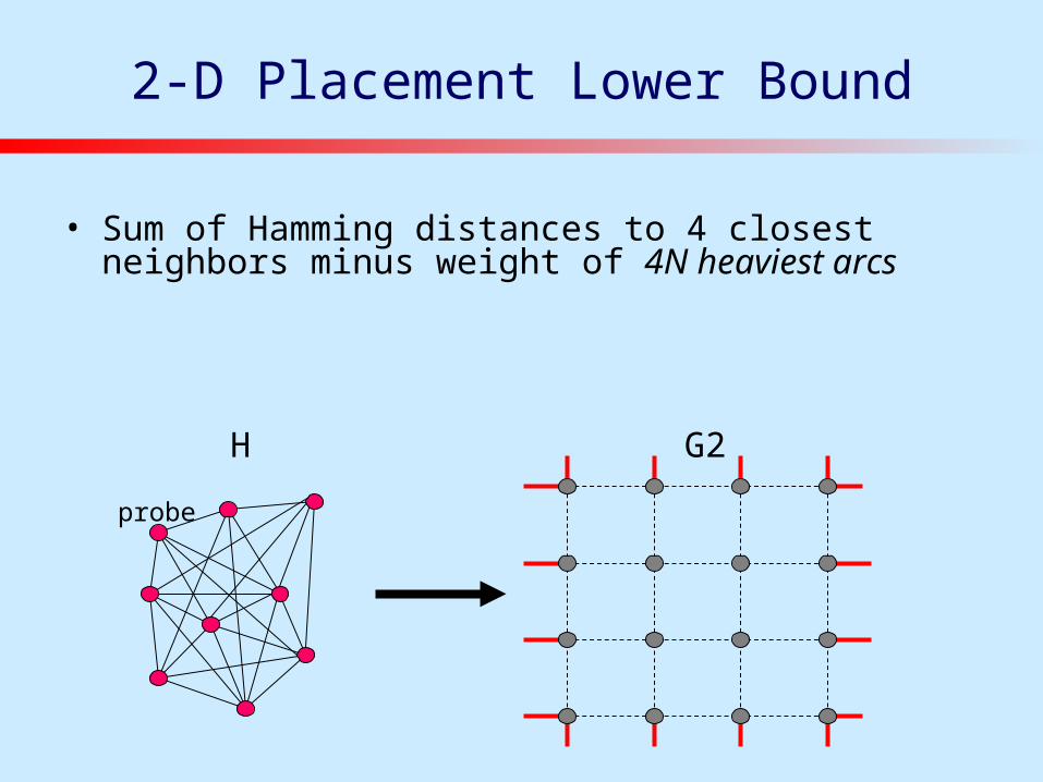
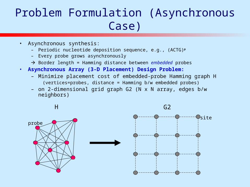
– Minimize placement cost of embedded-probe Hamming graph H (vertices=probes, distance = Hamming b/w embedded probes)
– on 2-dimensional grid graph G2 (N x N array, edges b/w neighbors)
H
probe
G2
site
Lower Bound
• Sum of distances to 4 closest neighbors minus weight of 4N heaviest arcs– Distance between two probes of length p = 2p - |Longest Common Subsequence|
• Non-tight bound: example with LB = 8 and best placement cost = 10
2M
5M
4M
AC
CT TG
GA
Optimum placement
AC
CT TG
GA1
1
1
1
1 111
Nuc
leot
ide
depo
sitio
n se
quen
ce S
=A
CT
GA
A
G
T
C
A
3M
1M
A
G
G
TT
C
C
A
(c)
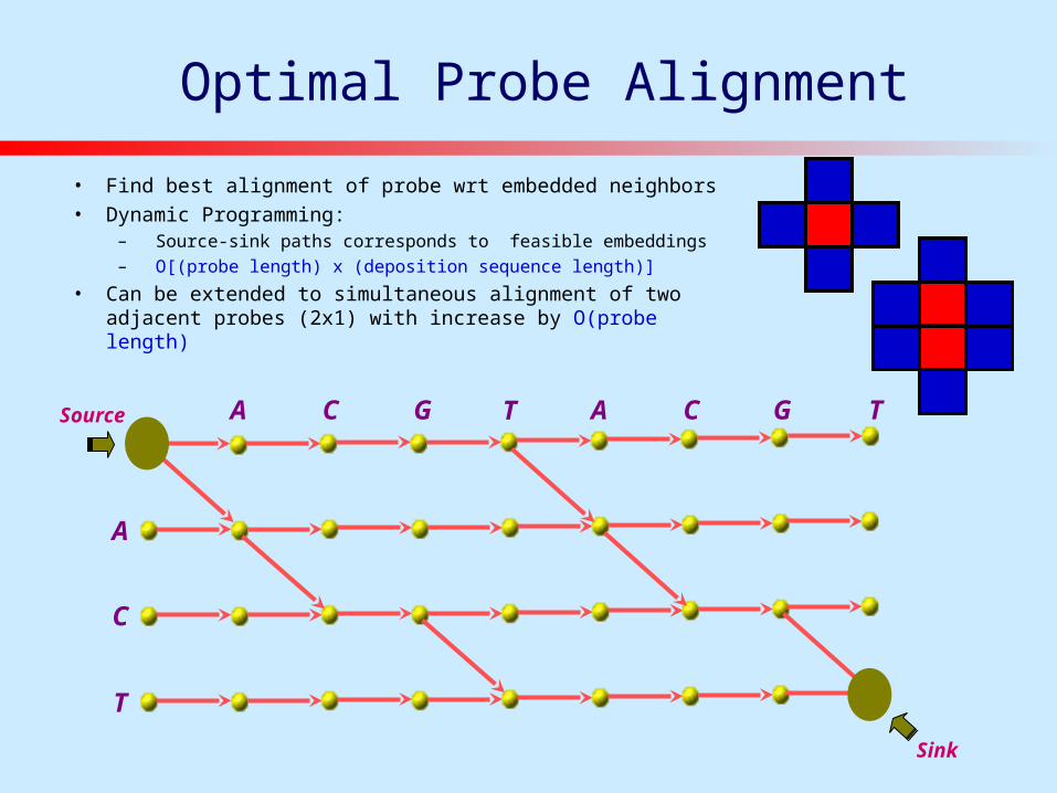
Optimal Probe Alignment
A
C
T
A C G T A C G TSource
Sink
• Find best alignment of probe wrt embedded neighbors• Dynamic Programming:
– Source-sink paths corresponds to feasible embeddings
– O[(probe length) x (deposition sequence length)]
• Can be extended to simultaneous alignment of two adjacent probes (2x1) with increase by O(probe length)
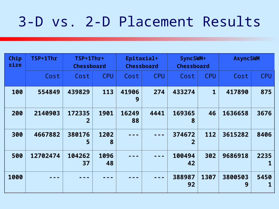
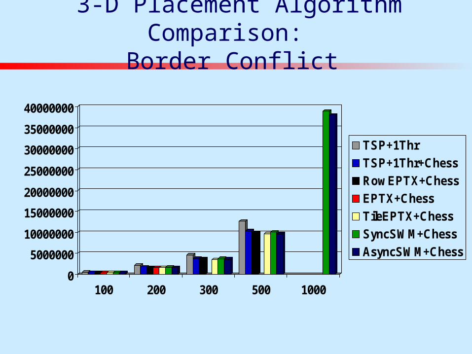
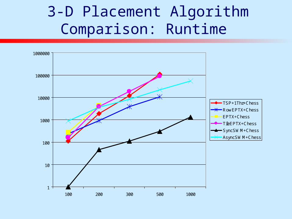
3-D Placement Flows
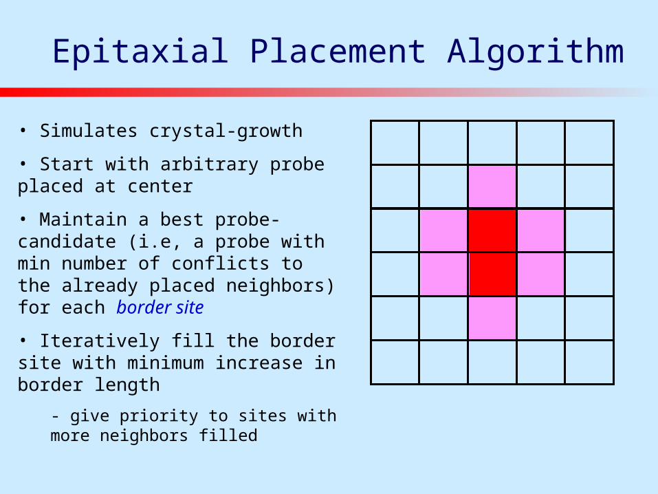
- Simultaneous placement and alignment- asynchronous epitaxial (slow and low quality)
- Synchronous placement followed by in-place probe alignment (analogous to standard for VLSI flow partition)- using previous DP to do in-place probe alignment
- Synchronous placement followed by probe alignment with reshuffle (analogous to feedback loops in VLSI flows)- asynchronous sliding window matching
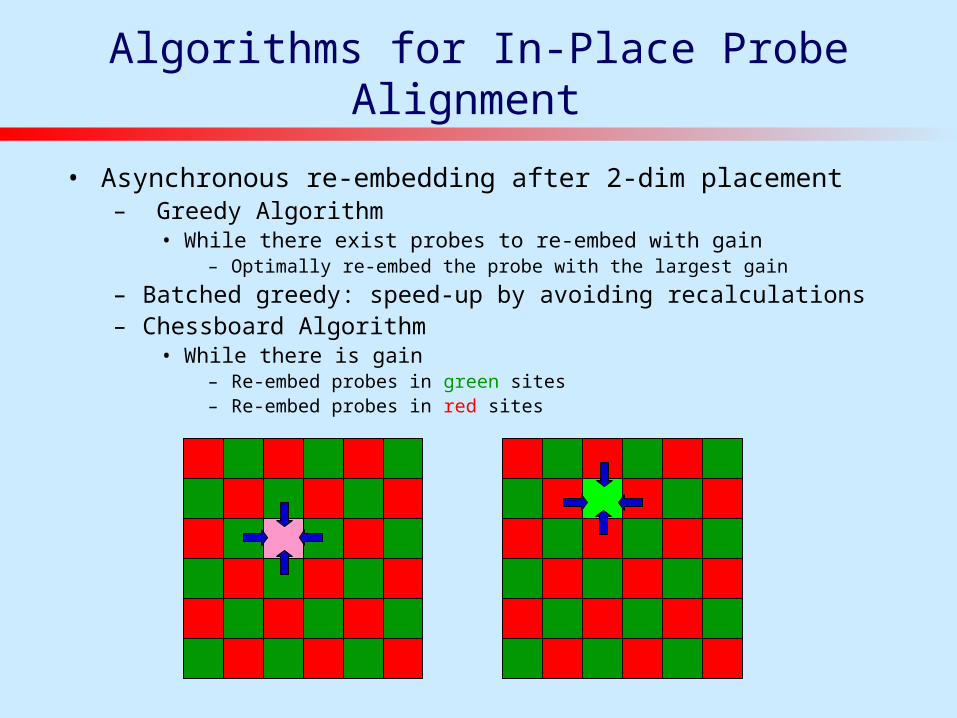
Algorithms for In-Place Probe Alignment
• Asynchronous re-embedding after 2-dim placement– Greedy Algorithm
• While there exist probes to re-embed with gain– Optimally re-embed the probe with the largest gain
– Batched greedy: speed-up by avoiding recalculations– Chessboard Algorithm
• While there is gain– Re-embed probes in green sites– Re-embed probes in red sites
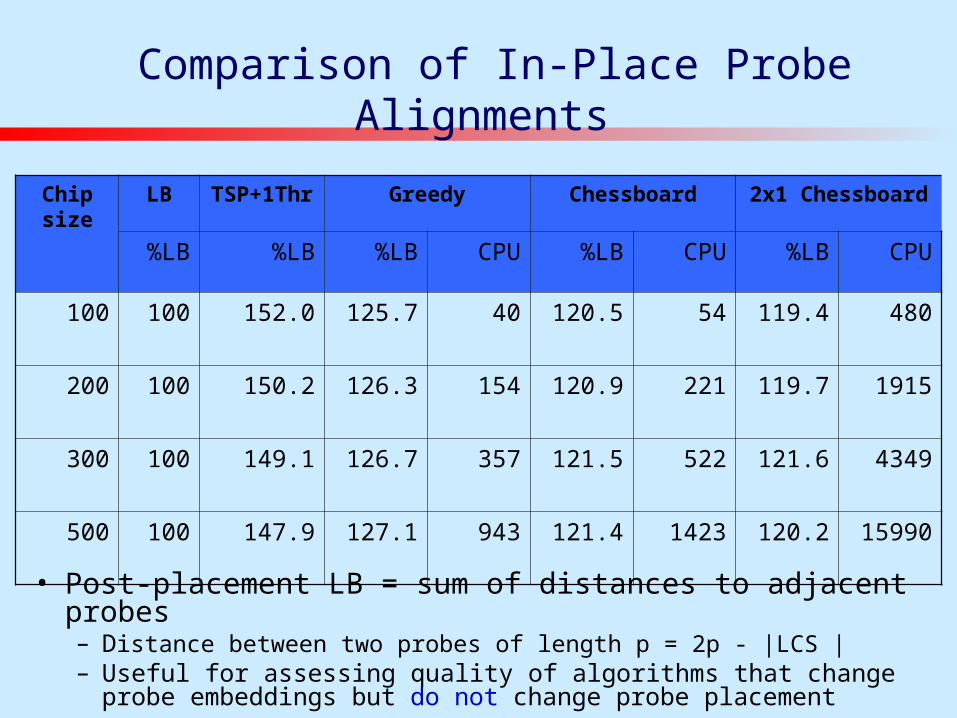
Comparison of In-Place Probe Alignments
Chip size
LB TSP+1Thr Greedy Chessboard 2x1 Chessboard
%LB %LB %LB CPU %LB CPU %LB CPU
100 100 152.0 125.7 40 120.5 54 119.4 480
200 100 150.2 126.3 154 120.9 221 119.7 1915
300 100 149.1 126.7 357 121.5 522 121.6 4349
500 100 147.9 127.1 943 121.4 1423 120.2 15990
• Post-placement LB = sum of distances to adjacent probes– Distance between two probes of length p = 2p - |LCS |– Useful for assessing quality of algorithms that change probe
Take into account conflicts between 2-,3-hop neighbors rather than only immediate neighbors
• Position-dependent border conflict weights
In alignment DP for two sequences take into account importance of conflicts in the middle of probes – alignment cost has weights on conflicts which depend on conflict position
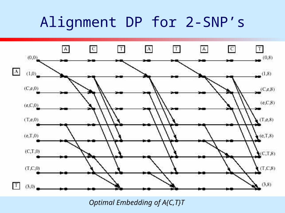
• Polymorphic probes
Chip contains SNP’s, e.g. pairs of probes different in a single position – they should be placed together and alignment DP should align them simultaneously
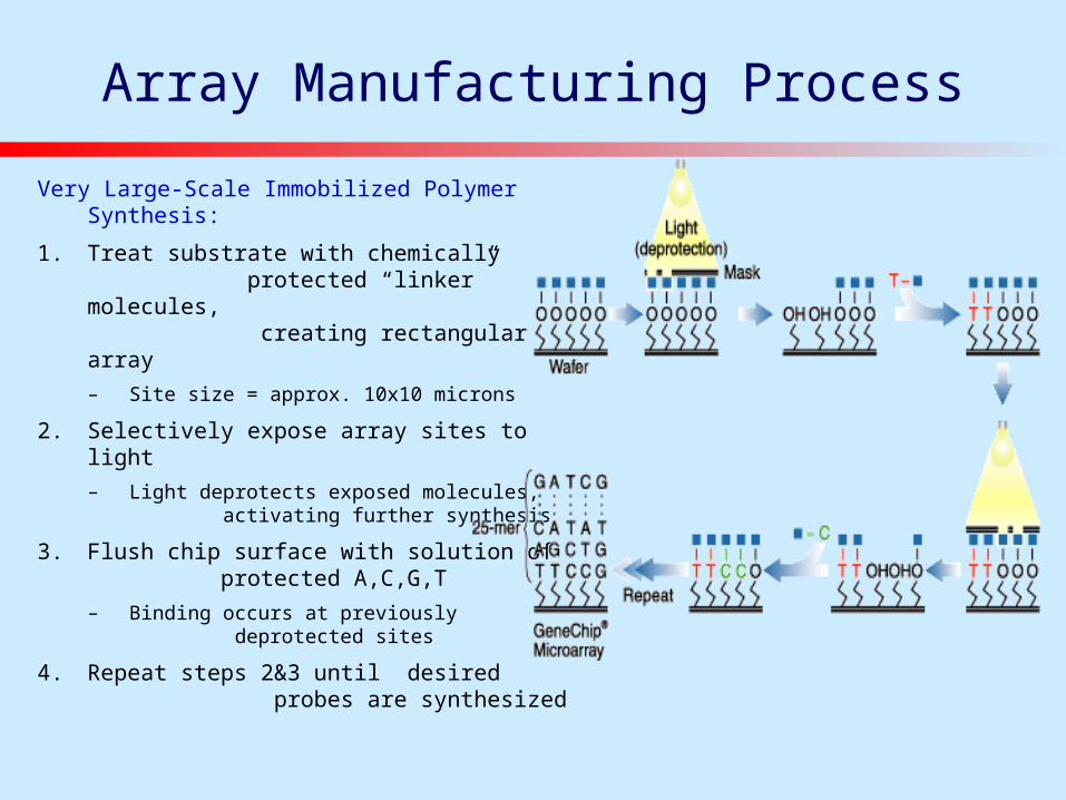
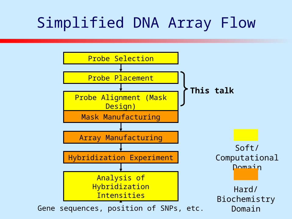
Simplified DNA Array Flow
Probe Selection
Probe Placement
Probe Alignment (Mask Design)
Array Manufacturing
Hybridization Experiment
Gene sequences, position of SNPs, etc.
This talk
Analysis of Hybridization Intensities
Mask Manufacturing
Soft/Computational Domain
Hard/Biochemistry Domain
Alignment DP for 2-SNP’s
Optimal Embedding of A{C,T}T
Summary
• Contributions:– Epitaxial placement reduces by extra 10% over the previously best
known method– Asynchronous placement problem formulation– Postplacement improvement by extra 15.5-21.8%– Lower bounds– Scalable Placements (1000x1000 in 20min)
• Ongoing work– Comparison on industrial benchmarks– Experiments with algorithms for extended formulations (SNPs,