Page 1
I
TÍTULO DE LA TESIS
Junio de 2014
León, Guanajuato,
México
GRADO EN QUE SE PRESENTA LA TESIS
GRADO EN QUE SE PRESENTA LA TESIS
Asesor(es):
Estudiante:
MAESTRÍA EN CIENCIAS (ÓPTICA)
ENGINEERING OF FOCAL FIELDS
USING VECTORIAL OPTICAL FIELDS
January 2017
León, Guanajuato, México
Advisor: Dr. Rafael Espinosa Luna Co-advisor: Dr. Qiwen Zhan
Student: Ing. Jason Eduardo Gómez Jamaica
Advisor: Dr. Rafael Espinosa Luna Co-advisor: Dr. Qiwen Zhan
Student: Ing. Jason Eduardo Gómez Jamaica
ENGINEERING OF FOCAL FIELDS
USING VECTORIAL OPTICAL FIELDS (Final version, changes suggested by advisors are included)
Page 3
I
Dedicatory
Este trabajo es dedicado a mi querida familia, es decir, mi padre quien siempre ha estado cuando lo
necesito y que sin importar las circunstancias me da ánimos para seguir adelante, mi madre quien
siempre ha hecho y dado todo para que yo esté bien y mis hermanos Jonathan, Jeremy y Jacob
quienes son lo más querido y para quienes siempre estaré.
Page 5
III
Acknowledgments
Firstly, I would like to thank to the Consejo Nacional de Ciencia y Tecnología, CONACyT, for
scholarship (339087) that made possible my Master’s degree. On the other hand, I also
render thanks to the Centro de Investigaciones en Óptica, A.C., for the academic
preparation that I obtained and I want to thank specially to my advisor Dr. Rafael Espinosa
Luna, my co-advisor Dr. Qiwen Zhan, my thesis reviewers Dr. Francisco Villa Villa and Dr.
Moisés Cywiak Garbarcewicz, my professor Dr. Alejandro Téllez Quiñones, my classmates
Oscar Naranjo, Etna Yáñez , Alan Bernal, Guadalupe López, Izcoatl Saucedo, Alan López,
Eduardo Rocko, Carlos Zamarripa, my friends Victor, Eusebio, Francisco, Wilson, Diana and
Felipe, and the admirable Dr. Efrain Mejia Beltran, which were a great support for me.
Page 7
V
Abstract
In this work is presented a revision of the main four theoretical methods employed for the
generation of longitudinally polarized beams of light. Results obtained by numerical
simulations using the method we consider the closest to our experimental capabilities are
presented. The source employed has associated an unconventional polarization distribution
corresponding to a radial polarization mode and although one can generate longitudinally
polarized beams by focusing a radially polarized light source with an aplanatic lens of high
numerical aperture, the strength of the longitudinal field component of these beams
decreases rapidly outside their waist. Therefore, we also present by numerical simulations
techniques to enhance the longitudinal field component of these beams, where different
radially polarized light sources were impinged on an annular diffractive optical element of
binary phase and then focused in a set-up of aplanatic high numerical aperture lenses, and
depending on the characteristics of the light source, the geometry of the diffractive optical
element, and the numerical aperture of the lenses, will be the beam dimensions and its
intensity profile. Thus, we achieved to obtain a non-diffracting longitudinally polarized
beam with FWHM=3.1λ, constant waist (0.88 λ) and a flat profile over most the covered
intensity area. Additionally, we have proposed an experimental method to verify the
existence of numerically simulated longitudinally polarized beams.
Page 9
VII
Table of contents
1. Introduction ---------------------------------------------------------------------------------- 1
2. Introduction to the polarization of the light ----------------------------------------- 3
2.1. Spatially uniform polarization states (conventional polarization) ----- 5
2.2. The Poincarè sphere --------------------------------------------------------------- 9
2.3. Spatially non-uniform polarization modes (unconventional
polarization) --------------------------------------------------------------------------- 11
2.4. Jones and Stokes matricial formalisms -------------------------------------- 14
3. Cylindrical vector beams ---------------------------------------------------------------- 20
3.1. Introduction ----------------------------------------------------------------------- 22
3.2. Mathematical description of cylindrical vector beams ------------------ 23
4. Generation of focal fields using optical vector fields ----------------------------- 27
4.1. Diffractive optical element, DOE --------------------------------------------- 27
4.2. Methods for creating specific focusing patterns ------------------------- 28
5. Results --------------------------------------------------------------------------------------- 37
5.1. Numerical simulations ---------------------------------------------------------- 37
5.2. Experimental results ------------------------------------------------------------- 48
6. Conclusions --------------------------------------------------------------------------------- 51
Appendix ------------------------------------------------------------------------------------------ 52 Bibliography ------------------------------------------------------------------------------------- 66
Page 11
IX
Symbols
Symbol Description Value and/or units |E | Electric field V/m
|D | Electric displacement field C/m2
|H | Intensity of magnetic field A/m
|B | Induction of magnetic field T
|J | Electric current density A/m2
|�� | Poynting vector W/m2
|𝐹 | Force N
|�� | instantaneous velocity of an electric charge m/s 𝑣 Speed of a wave through a medium m/s c Speed of light in the vacuum 3x10⁸ m/s
𝜆 Wavelength m 𝜎 Electric conductivity S/m 𝜇 Magnetic permeability H/m 휀 Electrical permittivity F/m 𝜌𝑞 Electric charge density C/m3
t Time s q Electric charge C 𝜌ξ Energy density J/ m3 𝐼𝑝𝑝 Intensity of the partially polarized light W 𝐼𝑐𝑝 Intensity of the completely polarized light W
Page 13
XI
Abbreviations
CV Cylindrical Vector
DOF Depth of Focus
BG Bessel-Gaussian
NA Numerical Aperture
DOE Diffractive Optical Element
FWHM Full Width at Half Maximum
3D Three-Dimensional
PP Polarization Plane
FF Focal Field
ULS Uniform Line Source
XZP xz-plane
MO Microscopy Objective
S-WP S-Waveplate
Page 15
CHAPTER 1-INTRODUCTION
1
Chapter 1
Introduction.
------------------------------------------------------------------------------------------------------------------------
------------------------------------------------------------------------------------------------------------------------
1. Introduction.
The polarization properties of light have been used as tools for different purposes,
ranging from basic research to application areas. Similarly, since the polarization
can be roughly divided in two types, conventional and unconventional polarization,
the applications areas are also divided. Therefore, one of the polarization modes in
the unconventional polarization is the mode with radial polarization. Where these
beams are currently used in three-dimensional focus engineering and due to its
unusual properties, these beams have been highly applied in research areas as
optical trapping and manipulation, particles acceleration, confocal microscopy,
fluorescent imaging, second-harmonic generation, Raman spectroscopy and high-
density optical data storage. Thus, the generation of specific focal fields has been
reported theoretically by employing four different methods, which use very
sophisticated techniques.
The first method consists of the incidence of a radially polarized Bessel-Gaussian
beam on a diffractive optical element to then be focused with a high numerical
aperture aplanatic-lens, and so it is generated, in the depth of focus region, a
longitudinally polarized optical needle with constant waist and length of 0.43λ and
4λ, respectively, which are dependent both of the numerical aperture and diffractive
optical element geometry [1, 2]. The second method consists of a focusing system,
where radially polarized beams are focused to create a spherical focal spot in the
focal region of the focusing system, in which different optical elements are analyzed
in order to generate focal spots with different profile shape [3, 4]. The third method
consist of the generation of a longitudinally polarized beam with super-Gaussian
profile and constant waist of 0.36λ, where these beams are generated by an incident
radially polarized beam in the optical arrangement with an annular paraboloid
mirror and a special filter, where it can be modulated its structural parameters in
order to generate a light needle (flat-top beam) length until 10λ [3, 4]. The last
method consists in obtaining a light needle with waist and length up to 0.36λ and
9.24λ, respectively, where the light needle is generated by reversing the electric field
pattern radiated from a different antennas in a 4Pi focusing system, and depending
on the numerical aperture of the aplanatic lenses of the 4Pi focusing system and the
Page 16
CHAPTER 1-INTRODUCTION
2
type and characteristics of the antenna, will be the dimensions of the generated light
needle [2].
Therefore, in order to propose an attainable and experimental method for
generating specific focal fields and at the same time verify the generated focal field
by numerical simulations, we studied in this thesis the four theoretical methods for
generating these fields, therefore we proposed a new and different method, which
consists of an incoming beam in a polarization converter and so this has a radial
polarization; when the beam is radially polarized, this passes through two optical
elements, a concentric two-belts diffractive optical element and a microscope
objective with numerical aperture of 0.90, and then is generated a longitudinally
polarized beam with flat intensity profile over most of the covered area, in other
words, a light needle is generated, which is located along the depth of field region
(DOF). Thus, if the light is generated in the depth of focus of the microscopy
objective, we could verify the existence of the light needle by using a vision system,
consisting on a CMOS camera and an image forming lens, where this system can be
displaced along the optical axis in order to verify the focal field formed in the DOF,
so this field could be scanned registering the images of the object at different
positions.
Page 17
CHAPTER 2-INTRODUCTION TO THE POLARIZATION OF LIGHT
3
Chapter 2
Introduction to the polarization of light.
------------------------------------------------------------------------------------------------------------------------
2.1. Spatially uniform polarization states (conventional
polarization)
2.2. The Poincarè sphere
2.3. Spatially non-uniform polarization modes (unconventional
polarization)
2.4. Jones and Stokes matricial formalisms
------------------------------------------------------------------------------------------------------------------------
2. Introduction to the polarization of the light.
One of the keywords in this work is "polarization of light", therefore, before its definition, a
short description of its origin will be provided.
Physics is the science focused to the study of the behavior and properties of matter and
energy, and interaction between them. Physical studies are divided in branches that are,
mechanics, thermodynamics, acoustics, electromagnetism, optics, and modern physics.
Optics studies the light and its interaction with matter. Depending on the conditions of the
generation and propagation of light and its interaction with matter, it is divided in three big
branches, which are, geometric optics, physics optics, and optoelectronics. Each branch
analyzes the beam differently, namely, like a propagating ray in the case of the geometric
optics, like a particle (photon) in the case of the optoelectronics and finally, like a wave in
the case of the optical physics approximation.
In this thesis, the polarization of light will be described using the physical optics
approximation, where the light is considered as a monochromatic plane traveling wave and
whose interactions with matter involve only linear optical responses.
For the study of the physical optics approximation, the beam is studied more specifically
like an electromagnetic wave. This electromagnetic wave can be represented as the
combination of two vectorial fields. The electric “E” and magnetic “H” fields. These fields
are mutually perpendicular and orthogonal to the propagation vector “𝑆” of the wave Fig.
(1), and it is supposed that the electromagnetic waves are propagated in the vacuum, or
another dielectric media.
Page 18
CHAPTER 2-INTRODUCTION TO THE POLARIZATION OF LIGHT
4
Figure 1. Representation of the orthogonal vector field components, E and H , in an electromagnetic
wave propagating along the 𝑆 direction.
The propagation vector is well-known as Poynting vector 𝑆 and whose modulus |𝑆 |
represents the instantaneous intensity of the electromagnetic energy that flows through a
surface perpendicular to the propagation direction of the wave:
𝑆 = �� × �� . (2.1)
The electromagnetic waves can have a property that will be named "Polarization", that
takes account of the orientation of the electric and magnetic field as the wave propagates
in the space.
Although the magnetic field could be used to represent the polarization of light, the main
reason to using only the electric field is that the strength of electric field is "c" times the
field strength of magnetic intensity field. Namely, the interaction of the magnetic field at
optical frequencies is rather weak so, the value of the energy density and the force (Lorentz
force) exerted by electromagnetic fields, 𝜌ξ and 𝐹 respectively, have much greater
contribution due to the electric field:
𝜌ξ =1
2(�� ∙ �� + �� ∙ �� ) . (2.2)
𝐹 = 𝑞(�� + �� × �� ) . (2.3)
Where �� and �� represent the displacement vector and the magnetic induction, 𝑞 is the
electric charge, and �� is the instantaneous velocity vector of the electric charge.
Page 19
CHAPTER 2-INTRODUCTION TO THE POLARIZATION OF LIGHT
5
2.1. Spatially uniform polarization states (conventional polarization)
Since the light is an electromagnetic wave that has a dependence in space and time, is
possible describe it in terms of the electric field �� . Thus, the electric field can be taken as
the superposition of the two mutually orthogonal fields, 𝐸𝑥 and 𝐸𝑦
, that travel on the same
direction and whose phase difference, 𝛿𝑥 − 𝛿𝑦, determines the polarization state.
�� = 𝐸𝑥 + 𝐸𝑦
. (2.1.1)
The 𝐸𝑥 and 𝐸𝑦
vectors oscillate on the 𝑥𝑧 and 𝑦𝑧 planes, respectively.
𝐸𝑥 = 𝐸0𝑥 𝑒
𝑖(𝜔𝑡−𝑘𝑧+𝛿𝑥) 𝑒�� . (2.1.2)
𝐸𝑦 = 𝐸0𝑦 𝑒
𝑖(𝜔𝑡−𝑘𝑧+𝛿𝑦) 𝑒�� . (2.1.3)
Thus, the electric field �� has associated an angular frequency 𝜔 and a wavenumber 𝑘. On
the other hand, �� also has temporal 𝑡 and spatial 𝑧 dependence, so �� =�� (𝑡, 𝑧), and 𝐸0𝑥,
𝛿𝑥, 𝑒�� and 𝐸0𝑦, 𝛿𝑦, 𝑒�� are the amplitudes, phases and unit vectors of the 𝐸𝑥 and 𝐸𝑥
fields,
respectively.
The trajectory described by the end of the electric field in the space can be described
alternatively at a fixed point as a function of time, or it can be described at a fixed time as
a function of the spatial coordinates. The polarization of the light can be classified into five
categories, which are known as “polarization states” with spatially uniform distributions of
the amplitude and phase.
Linear polarization (first category).
The linearly polarized state can be described as the superposition of two orthogonal electric
fields, 𝐸𝑥 and 𝐸𝑥
, traveling along the same direction 𝑆 (propagation vector) and having a
phase difference 𝛿 of 0 degrees, that is, 𝛿𝑦 − 𝛿𝑥 = 0. On the other hand, the electric field
�� oscillates along a same plane, which will be named 𝑃𝑃 (polarization plane) and the value
of the amplitudes of the 𝐸𝑥 and 𝐸𝑥
fields will depend on the orientation of the polarization
plane around the optical axis 𝑧, where all the electric field vectors oscillate on the
polarization plane, which is fixed to an angle θ with respect to the XZP (𝑥𝑧-plane), described
within a Cartesian coordinate system (𝑥, 𝑦, 𝑧). This description is reported observing to the
source.
For simplicity, the direction of the 𝑆 vector has been chosen to be parallel to the 𝑧 axis Fig.
(2).
Page 20
CHAPTER 2-INTRODUCTION TO THE POLARIZATION OF LIGHT
6
a) Linear (p)-polarization state b) Linear (+45 degrees)-polarization state
c) Linear (s)-polarization state d) Linear (-45 degrees)-polarization state
e) Linear (θ)-polarization state
Figure 2. Linearly polarized states under different tilt angles of the polarization plane (considering
the tilt angles of the polarization plane with respect to the XZP). a) 𝑃𝑃 to 0 degrees, where this
polarization state is well-known as (p)-polarization and (p) means paralelle, which comes from the
German language. b) PP to 45 degrees, where this polarization state is known as (+45 degrees)-
polarization and (+45 degrees) stands for the tilt angle of the PP to 45 degrees. c) PP to 90 degrees,
where this polarization state is well-known as (s)-polarization and (s) means senkrecht, which comes
from the German language. d) PP to -45 degrees, where this polarization state is known as (-45
degrees)-polarization and (-) stands for the tilt of the PP to 45 degrees. e) PP to a θ (any angle),
where this polarization state is known as (θ)-polarization and θ stands for the tilt of the PP to a θ.
Circular polarization (Second category).
Page 21
CHAPTER 2-INTRODUCTION TO THE POLARIZATION OF LIGHT
7
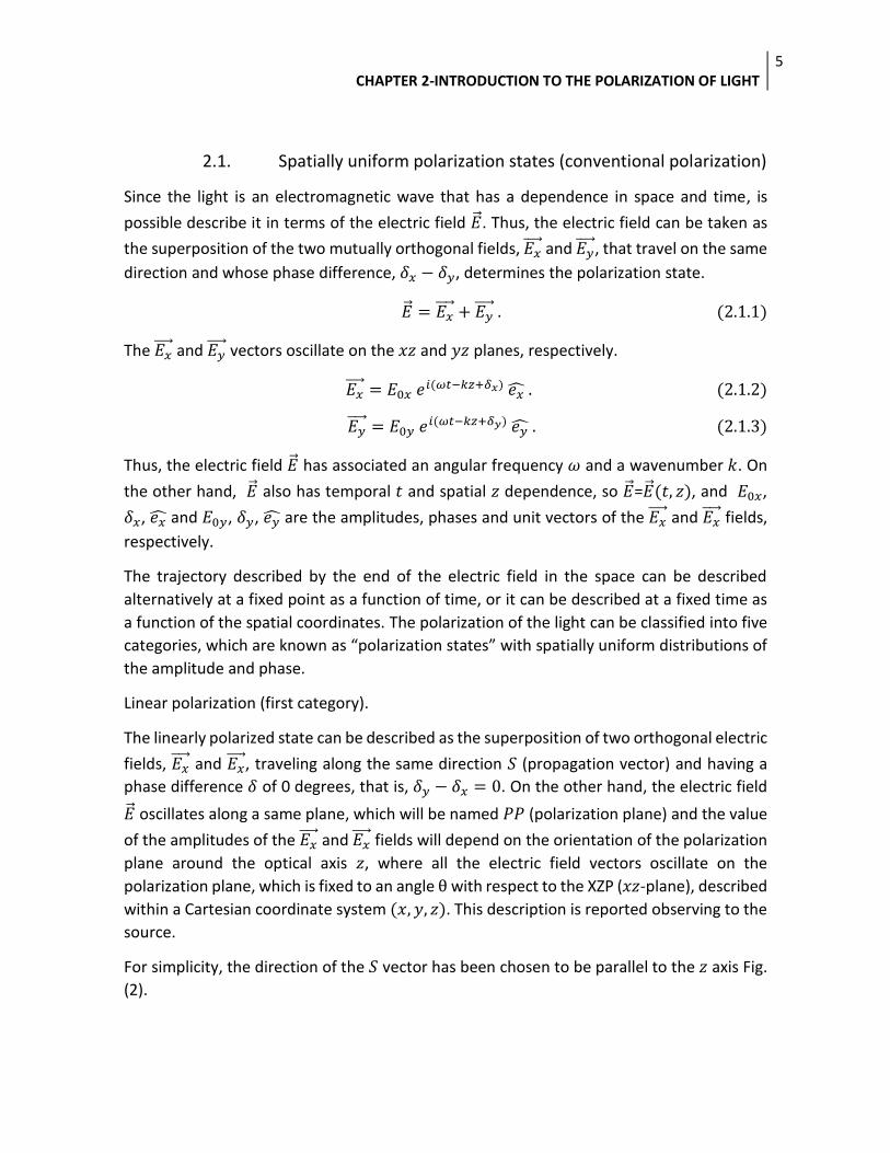
The circularly polarized state can be described as the superposition of the two orthogonal
electric fields, 𝐸𝑥 and 𝐸𝑦
, with equal amplitudes (𝐸𝑥 = 𝐸𝑦), traveling along the same
direction, and whose phase difference δ between the orthogonal electric components is of
±90 degrees. If the value of δ is +90 degrees, 𝐸𝑥 and 𝐸𝑦
rotates at clockwise, and the
resultant electric field �� describes a complete circle after a period of a wavelength; this
state is named “circular right-hand polarization”. Otherwise, If the δ is -90 degrees, 𝐸𝑥 and
𝐸𝑦 rotate at counter-clockwise, and the resultant electric field describes a complete circle
after a period of a wavelength; this state is named “circular left-hand polarization”. On the
other hand, the electric field �� oscillates along a different plane, which will be named 𝑃𝑃
(polarization plane) and depending of the value of the amplitudes of the 𝐸𝑥 and 𝐸𝑥
fields,
will be the orientation of the polarization plane around the optical axis 𝑧. Therefore, for
each electric field vectors �� , there is a single polarization plane, that is, a 𝐸 vector set,
where each one of them will be located on a polarization plane to an angle θ with respect
to the XZP (𝑥𝑧-plane), described within a Cartesian coordinate system (𝑥, 𝑦, 𝑧). This
description is reported observing to the source.
The aforementioned 𝐸 vector set is generated by the angular motion of a single vector 𝐸
that traveling along the 𝑧 optical axis. This motion can be modeled completely as a
cylindrical helix with constant radius, that is, a helical motion.
Note that the direction of the 𝑆 vector is along the 𝑧 axis Fig (3).
a) Circular (L)-polarization state b) Circular (R)-polarization state
Figure 3. Circularly polarized states with both rotations. a) Circular polarization state at counter-
clockwise with respect to the 𝑆 direction, where this polarization state is well-known as (L)-
polarization and “L” stands for “Left hand”, which means that the 𝐸 vector rotates at counter-
clockwise. b) Circular polarization state at clockwise with respect to the 𝑆 direction, where this
polarization state is well-known as (R)-polarization and “R” stands for “Right hand”, which means
that the 𝐸 vector rotates clockwise.
Elliptical polarization (third category).
Page 22
CHAPTER 2-INTRODUCTION TO THE POLARIZATION OF LIGHT
8
The elliptically polarized state can be described as the superposition of the two orthogonal
electric fields, 𝐸𝑥 and 𝐸𝑦
, with different amplitudes (𝐸𝑥 ≠ 𝐸𝑦), traveling along the same
direction, and whose phase difference δ between the orthogonal electric components, can
take any value, except 0 and ∓90 degrees. If the value of δ is positive, 𝐸𝑥 and 𝐸𝑦
rotates
clockwise, and the resultant electric field �� describes a complete circle after a period of a
wavelength; this state is named “elliptical right-hand polarization”. Otherwise, If the δ is
negative, 𝐸𝑥 and 𝐸𝑦
rotate counter-clockwise, and the resultant electric field describes a
complete ellipse after a period of a wavelength; this state is named “elliptical left-hand
polarization”. The electric field �� oscillates in a plane called the 𝑃𝑃. Therefore, for each
electric field vector �� , there will be a single 𝑃𝑃, that is, a 𝐸 vector set where each one of
them will be located on a 𝑃𝑃 to different slope with respect to the XZP (𝑥𝑧-plane), described
within a Cartesian coordinate system (𝑥, 𝑦, 𝑧). This description is reported observing to the
source.
The aforementioned 𝐸 vector set is generated by the angular motion of a single vector 𝐸
traveling along the 𝑧 optical axis. This motion can be modeled completely as a cylindrical
helix with variable radius, that is, a helical motion.
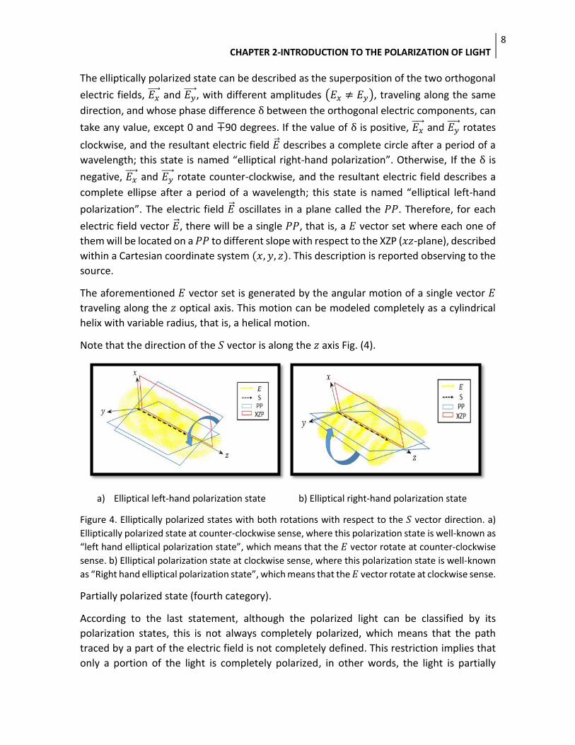
Note that the direction of the 𝑆 vector is along the 𝑧 axis Fig. (4).
a) Elliptical left-hand polarization state b) Elliptical right-hand polarization state
Figure 4. Elliptically polarized states with both rotations with respect to the 𝑆 vector direction. a)
Elliptically polarized state at counter-clockwise sense, where this polarization state is well-known as
“left hand elliptical polarization state”, which means that the 𝐸 vector rotate at counter-clockwise
sense. b) Elliptical polarization state at clockwise sense, where this polarization state is well-known
as “Right hand elliptical polarization state”, which means that the 𝐸 vector rotate at clockwise sense.
Partially polarized state (fourth category).
According to the last statement, although the polarized light can be classified by its
polarization states, this is not always completely polarized, which means that the path
traced by a part of the electric field is not completely defined. This restriction implies that
only a portion of the light is completely polarized, in other words, the light is partially
Page 23
CHAPTER 2-INTRODUCTION TO THE POLARIZATION OF LIGHT
9
polarized or is not completely polarized. Therefore, the combination between a completely
polarized state and an unpolarized state, results a partially polarized state, which has
associated a DoP (degree of polarization) and can be represented by:
𝑆 = (
𝑆0
𝑆1
𝑆2
𝑆3
) = (1 − 𝐷𝑜𝑃)(
𝑆0
000
) + 𝐷𝑜𝑃 (
𝑆0
𝑆1
𝑆2
𝑆3
) . (2.1.4)
Where 𝑆0, 𝑆1, 𝑆2 and 𝑆3 are elements of the Stokes vector, in which the 𝑆1, 𝑆2 and 𝑆3
parameters represent a specific polarization state with total intensity indicated by the 𝑆0
parameter. On the other hand, the DoP for completely polarized light is one (DoP=1), for
unpolarized light the DoP is zero (DoP=0), and as mentioned above, for partially polarized
light the DoP varies between zero and one (0 < DoP < 1). Thus, the DoP can be represented
mathematically as:
𝐷𝑜𝑃 =𝐼𝑐𝑝
𝐼𝑝𝑝=
√𝑆12 + 𝑆2
2 + 𝑆32
𝑆0 . (2.1.5)
Where 𝐼𝑝𝑝 and 𝐼𝑐𝑝 are the intensities of the partially and completely polarized light,
respectively. Therefore, if the light is completely or partially polarized, the Stokes vector
parameters meet certain relationships between them:
Completely polarized light 𝑆02 = 𝑆1
2 + 𝑆22 + 𝑆3
2 . (2.1.6)
Partially polarized light 𝑆02 > 𝑆1
2 + 𝑆22 + 𝑆3
2 . (2.1.7)
Non-polarized state (last category).
Thus, the behavior and the description of the electric field of light by the end is known as
“polarization of the light” and is represented by the path traced the electric field vector.
However, when the path traced by the electric field describes a random orientation, it is
said that light is not polarized, which means that amplitude and phase vary randomly in
space and time.
2.2. The Poincarè sphere
As previously stated above, the polarization states can be represented by the Stokes
vector, which can be written as:
𝑆 = (
𝑆0
𝑆1
𝑆2
𝑆3
) . (2.2.1)
Page 24
CHAPTER 2-INTRODUCTION TO THE POLARIZATION OF LIGHT
10
Whose parameters can be represented like a point that is located in a sphere, which is
named “Poincarè sphere”, Fig. (5).
Figure 5. Representation of the Poincarè sphere
Where 𝑆1, 𝑆2 and 𝑆3 are parameters that indicate the values of the axes in a sphere, with
an unity radius.
Then, for a totally polarized state, the point (𝑠1,𝑠2,𝑠3) is on the surface of the sphere and
for a partially polarized state, the point (𝑠1,𝑠2,𝑠3) is inside it. Another way to represent a
polarization state in the Poincarè sphere, is by means of the orientation and ellipticity
angles, ψ and χ, respectively, which can be represented in the sphere as shown in the
following figure.
Figure 6. Representation of the ψ and χ angles in the Poincarè sphere.
Where ψ and χ are angles that depend also of the amplitudes and phases of the orthogonal
components of the electric field, and they can be represented mathematically as:
tan(2𝜓) = 2𝐸0𝑥𝐸0𝑦
𝐸0𝑥2 − 𝐸0𝑦
2 cos(𝛿) . (2.2.2)
With (0 ≤ 𝜓 ≤ 𝜋).
Page 25
CHAPTER 2-INTRODUCTION TO THE POLARIZATION OF LIGHT
11
sin(2χ) = 2𝐸0𝑥𝐸0𝑦
𝐸0𝑥2 + 𝐸0𝑦
2 sin(𝛿) . (2.2.3)
With χ between - 𝜋/4 and 𝜋/4, that is, (−𝜋
4≤ χ ≤
𝜋
4) .
2.3. Spatially non-uniform polarization modes (unconventional
polarization).
In optics, when one analyzes a polarization state of light, it also is usually assumed that the
cross section of the light beam has spatially homogeneous polarization, that is, the
polarization is studied conventionally. However, there are beams whose polarization is not
spatially homogeneous and this property of light gave rise to new phenomena and
applications, in what is called unconventional polarization.
As it was previously mentioned, the path traced by the end of the electric field can be
represented by polarization states, where the spatial distribution of the electric field is
uniform, that is, all electric field vectors associated with each point on a lighting region (light
spot), have equal direction and sense Fig. (1). Thus, when the inner product between an
arbitrary vector and all �� is equal to the product of the modules of said vectors, the
polarization is known as conventional, that is, “Conventional polarization”.
Assuming that the degree of polarization is unity (DoP=1).
Figure 1. Conventional polarization
However, the spatial distribution of the electric field, it is not always uniform, entailing to
the existence of a new type of polarization, which is known as “Non-conventional
polarization” Fig. (2), where not all vectors of the field �� have equal direction and sense,
implying that the inner product between an arbitrary vector and any other element of the
vectorial field �� is different to the product of the modules of said vectors.
Page 26
CHAPTER 2-INTRODUCTION TO THE POLARIZATION OF LIGHT
12
Figure 2. Unconventional polarization
Thus, the linear superposition of light with unconventional polarization generates
unconventional polarization states, which are known as polarization modes and are
spatially non-uniform. An elementary Gaussian beam with linear polarization has oriented
its electric field components along a unique direction and sense, see Fig. 3(a). In contrast to
the best known spatial distributions, which are the Hermite-Gauss (HG) and the Laguerre-
Gauss (LG) modes with linear polarization, with their electric field vectors oscillating in same
direction but in different sense, Figs. 3(b)-3(f). Of particular importance to us, are the
unconventional distributions with electric field vectors directed around the radial and the
azimuthal direction, which are named modes with radial and azimuthal polarization,
respectively, and are represented in Figs. 3(g) and 3(h); when these two modes are
superimposed linearly, they give rise to the mode with spiral polarization, which is found in
the Fig. 3(i) and represented the unconventional state of a generalized cylindrical vector-
beam [19].
Page 27
CHAPTER 2-INTRODUCTION TO THE POLARIZATION OF LIGHT
13
Figure 3. Best known spatially non-uniform polarization modes compared with the polarization state
of an elementary Gaussian beam: (a) 𝑥-polarized elementary Gaussian beam, (b) 𝑥-polarized HG10
mode, (c) 𝑥-polarized HG01 mode, (d) 𝑦-polarized HG01 mode, (e) 𝑦-polarized HG10 mode, (f) 𝑥-
polarized LG0 mode, (g) mode with radial polarization, (h) mode with azimuthal polarization, (i)
mode with spiral polarization. Figure taken from [19].
The subscripts of the HG modes indicate the degree of the probabilistic Hermite
polynomials both 𝑥 and 𝑦; in the same way, the subscript of the LG mode indicates the
degree of the generalized Laguerre polynomials 𝐿1(⋯ ).
Similarly, the radially and azimuthally polarized modes are represented as the linear
superposition of a 𝑥-polarized HG10 mode with a 𝑦-polarized HG01 mode and a 𝑥-polarized
HG01 mode and a 𝑦-polarized HG10 mode, respectively, which shown in Fig. (4) and can be
represented mathematically as [19]:
�� 𝑟 = 𝐻𝐺10 𝑒 𝑥 + 𝐻𝐺01 𝑒 𝑦 . (2.3.1)
�� 𝜙 = 𝐻𝐺01 𝑒 𝑥 + 𝐻𝐺10 𝑒 𝑦 . (2.3.2)
Where �� 𝑟 and �� 𝜙 are electric fields with radial and azimuthal polarization, respectively.
Page 28
CHAPTER 2-INTRODUCTION TO THE POLARIZATION OF LIGHT
14
Figure 4. Radially and azimuthally polarized modes by the linear superposition of the different HG
modes. Figure taken from [19].
2.4. Jones and Stokes matricial formalisms.
The light (electromagnetic waves) can be classified in terms of its polarization state, and it
is possible to represent the light mathematically by two different formalisms known as
Jones and Stokes matricial formalisms.
Jones matrix formalisms (first formalism).
In this formalism the polarization states of the totally polarized light are represented as a
column vectors of dimensions 2×1, which can be represented by the orthogonal
components, 𝐸𝑥 and 𝐸𝑦
, where depending of the value amplitudes, E0x and E0y, and the
phase difference (𝛿 = 𝛿𝑦 − 𝛿𝑥) between these components, will represent the polarization
state of the electric field �� . This description is reported observing to the source.
Such column vector is known as a “Jones vector”:
Jones vector �� = (𝐸cos (θ)𝑒𝑖𝛿𝑥
𝐸sin(θ)𝑒𝑖𝛿𝑦) . (2.4.1)
Where θ indicates the angle between the electric field �� and one of its orthogonal
components (Ex , 𝐸𝑦
). Therefore, the Jones vector can be written in terms of the amplitude
values of the orthogonal components:
Page 29
CHAPTER 2-INTRODUCTION TO THE POLARIZATION OF LIGHT
15
�� = (E0x
E0y𝑒𝑖δ) . (2.4.2)
The Jones vectors also can be represented by:
�� = 𝐸𝑥 + 𝐸𝑦
. (2.4.3)
With 𝐸𝑥 = E0x 𝑒
𝑖(𝜔𝑡−𝑘𝑧) 𝑒�� and 𝐸𝑦 = E0y 𝑒
𝑖(𝜔𝑡−𝑘𝑧+𝛿) 𝑒��; where 𝐸𝑥 and 𝐸𝑦
travel along a
same direction, and for simplicity the vectorial components are in the direction S associated
to the propagation direction (along the 𝑧 axis, according to the Fig. (5)), which is
perpendicular to the electric field.
Figure 5. Vector of the electric field �� to an angle θ with respect to the 𝑥 axis, where its respective
orthogonal components 𝐸𝑥 and 𝐸𝑦
are traveling along the optical 𝑧 axis.
Therefore, each polarization state has associated a single Jones vector, which can be
represented by:
�� = (1
0) → (p) − linearly polarized state
�� = (0
1) → (s) − linearly polarized state
�� =1
√2 (
1
1) → (+45 degrees) − linearly polarized state
�� =1
√2 (
1
−1) → (−45 degrees) − linearly polarized state
�� = ( cos (θ)
sin(θ)) → (θ) − linearly polarized state
Where θ indicates any angle between the electric field �� and its components Ex .
�� =1
√2 (
1
𝑖) → (R) − Circularly right − hand polarized state
Page 30
CHAPTER 2-INTRODUCTION TO THE POLARIZATION OF LIGHT
16
�� =1
√2 (
1
−𝑖) → (L) − Circularly left − hand polarized state
�� = (E0y
𝑒±𝑖δ E0x) → Elliptically polarized state
𝑊𝑖𝑡ℎ �� =��
|�� |.
Although the traced path end of the electric field �� is well defined, the polarization state
could be changed depending on the interaction of light with matter (optical elements,
material samples or simply an object that polarizing the incident beam), and therefore each
object will have an associated matrix, and it is commonly known as “Jones Matrix”:
Jones matrix 𝐽 = (𝐽𝑥𝑥 𝐽𝑥𝑦
𝐽𝑦𝑥 𝐽𝑦𝑦) . (2.4.4)
Which depending of its values (𝐽𝑥𝑥, 𝐽𝑥𝑦, 𝐽𝑦𝑥 and 𝐽𝑦𝑦), will be the change in the polarization
state of the light beam that impinge on the object, and this physical behavior can be
represented by:
��𝑜 = 𝐽��𝑖 . (2.4.5)
Where ��𝑖 and ��𝑜 is the polarization state represents by the Jones notation, before and after
passing through the object, and 𝐽 represent the Jones matrix of any object. This assumption
is done considering a linear response to light.
Stokes matrix formalism (second formalism)
In this formalism the polarization states of the light, which may be totally polarized, partially
polarized, or totally unpolarized and these are represented as column vectors of dimensions
4×1, commonly known as “Stokes vector” 𝑆. The Stokes vector are also related to
observable quantities which are:
𝑆 = (
𝐼𝑝 + 𝐼𝑠𝐼𝑝 − 𝐼𝑠𝐼+ − 𝐼−𝐼𝑅 − 𝐼𝐿
) . (2.4.6)
Where 𝐼𝑝, 𝐼𝑠, 𝐼+ and 𝐼− represent the intensities of the linearly polarized electric field to 0,
90, 45 and -45 degrees, respectively, and 𝐼𝑅 and 𝐼𝐿 represent the intensities of the circularly
polarized electric field at clockwise and counter-clockwise sense, respectively (observing to
the source direction). Besides, these intensities also can be represented in function of the
amplitudes of the orthogonal components of the electric field �� (𝐸𝑥 and 𝐸𝑦) and their phase
difference, so the Stokes vector can be represented as:
Page 31
CHAPTER 2-INTRODUCTION TO THE POLARIZATION OF LIGHT
17
𝑆 =
(
𝐸𝑥𝐸𝑥∗ + 𝐸𝑦𝐸𝑦
∗
𝐸𝑥𝐸𝑥∗ − 𝐸𝑦𝐸𝑦
∗
𝐸𝑥𝐸𝑦∗ + 𝐸𝑦𝐸𝑥
∗
𝑖 (𝐸𝑥𝐸𝑦∗ − 𝐸𝑦𝐸𝑥
∗) )
. (2.4.7)
Therefore, each polarization state has associated a single Stokes vector, which can be
represented by:
𝑆 = (
1100
) → (p) − linearly polarized state
With E0x normalized to unity, and therefore |E0x|2 = 1
𝑆 = (
1−100
) → (s) − linearly polarized state
With E0y normalized to unity, and |E0y|2= 1
𝑆 = 2 (
1010
) → (+45 degrees) − linearly polarized state
With E0x normalized to unity, and |E0x|2 = 1
𝑆 = 2 (
10
−10
) → (−45 degrees) − linearly polarized state
With E0y normalized to unity, and |E0y|2= 1
𝑆 = (
1cos (2θ)
sin (2θ)0
) → (θ) − linearly polarized state
With E normalized to unity, |E|2 = 1, where �� = 𝐸𝑥 + 𝐸𝑦
and θ is the angle between the
electric field �� and its component 𝐸𝑦 .
𝑆 = 2 (
1001
) → (R) − Circularly right − hand polarized state
Page 32
CHAPTER 2-INTRODUCTION TO THE POLARIZATION OF LIGHT
18
With E0x normalized to unity, |E0x|2 = 1
𝑆 = 2 (
100
−1
) → (L) − Circularly left − hand polarized state
With E0x normalized to unity, |E0x|2 = 1
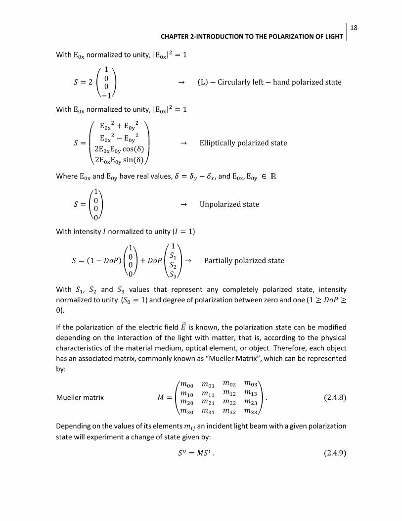
𝑆 =
(
E0x2 + E0y
2
E0x2 − E0y
2
2E0xE0y cos(δ)
2E0xE0y sin(δ))
→ Elliptically polarized state
Where E0x and E0y have real values, 𝛿 = 𝛿𝑦 − 𝛿𝑥, and E0x, E0y ∈ ℝ
𝑆 = (
1000
) → Unpolarized state
With intensity 𝐼 normalized to unity (𝐼 = 1)
𝑆 = (1 − 𝐷𝑜𝑃)(
1000
) + 𝐷𝑜𝑃 (
1𝑆1
𝑆2
𝑆3
) → Partially polarized state
With 𝑆1, 𝑆2 and 𝑆3 values that represent any completely polarized state, intensity
normalized to unity (𝑆0 = 1) and degree of polarization between zero and one (1 ≥ 𝐷𝑜𝑃 ≥
0).
If the polarization of the electric field �� is known, the polarization state can be modified
depending on the interaction of the light with matter, that is, according to the physical
characteristics of the material medium, optical element, or object. Therefore, each object
has an associated matrix, commonly known as “Mueller Matrix”, which can be represented
by:
Mueller matrix 𝑀 = (
𝑚00 𝑚01𝑚02 𝑚03
𝑚10 𝑚11 𝑚12 𝑚13
𝑚20
𝑚30
𝑚21
𝑚31
𝑚22 𝑚23
𝑚32 𝑚33
) . (2.4.8)
Depending on the values of its elements 𝑚𝑖𝑗 an incident light beam with a given polarization
state will experiment a change of state given by:
𝑆𝑜 = 𝑀𝑆𝑖 . (2.4.9)
Page 33
CHAPTER 2-INTRODUCTION TO THE POLARIZATION OF LIGHT
19
Where 𝑆𝑖 and 𝑆𝑜 are the polarization states represented by the Stokes notation, before and
after passing through the object.
Page 34
CHAPTER 3-CYLINDRICAL VECTOR-BEAMS
20
Chapter 3
Cylindrical vector-beams.
------------------------------------------------------------------------------------------------------------------------
3.1. Introduction
3.2. Mathematical description of cylindrical vector beams
------------------------------------------------------------------------------------------------------------------------
3. Cylindrical vector beams.
Electromagnetic waves are oscillatory disturbances caused by moving electric charges that
transfer energy and can be able to travel through any medium or vacuum, and their
existence can be demonstrated by the Maxwell’s equations:
Magnetic Gauss's law ∇ ∙ 𝜇H = 0 . (3.1)
Electric Gauss's law ∇ ∙ E =𝜌𝑞
. (3.2)
Faraday's law of induction ∇ × E = −𝜕𝜇H
𝜕𝑡 . (3.3)
Ampère's law ∇ × 𝜇H = 𝜇 (𝜎E + 휀𝜕E
𝜕𝑡) . (3.4)
(Which are expressed in the international system of units “SI”)
In these equations H is the vector of the intensity of the magnetic field, E is the electric
field, and 𝜌𝑞 is the electric charge density of the medium where the fields are propagated;
and whose properties 𝜇, 휀 and 𝜎 represent the magnetic permeability, the electrical
permittivity and electric conductivity of the medium, respectively.
The physical relationships that represent the response of the linear media under the
interaction with the fields are called commonly constitutive relationships:
B = 𝜇H . (3.5)
D = 휀E . (3.6)
J = 𝜎E . (3.7)
(These relationships suppose an isotropic and homogeneous medium, implying that 𝜇, 휀, 𝜎
are scalars)
Page 35
CHAPTER 3-CYLINDRICAL VECTOR-BEAMS
21
B is the magnetic induction field, D is the electric displacement field and is the responsible
for the effects of free and bound charges within a medium, and J is the electric current
density.
On the other hand, if H or E are analyzed like waves that travel through a isotropic and
homogeneous medium without electric charge density and electric conductivity , it is
possible to know the propagation of these fields by using the wave equation:
∇2 𝜓(r, 𝑡) −1
𝑣2
𝜕2
𝜕𝑡2𝜓(r, 𝑡) = 0 . (3.8)
Where 𝜓(r, 𝑡) is the wave function of the studied field, and whose function depends on the
position vector r and the time 𝑡. Such field is propagated through a medium to speed 𝑣,
which depends on the properties of said medium:
𝑣 =1
√𝜇휀 . (3.9)
Therefore, if the electric field has harmonic dependence over time, the wave can be
expressed mathematically as:
𝜓(r, 𝑡) = 𝐸(𝑟)𝑒−𝑖𝜔𝑡 . (3.10)
Where 𝐸(𝑟) is the amplitude of the electric field in function of the position 𝑟 traveling in
direction k , that is, the wave vector that points to the direction of propagation of the wave,
whose magnitude indicated the number of times that fits the wavelength “λ” of the wave
of electric field in a cycle (𝑘 = 2𝜋/𝜆) and also represents the ratio between the angular
frequency and the speed of the wave in the medium (𝑘 = 𝜔/𝑣).
Thus, if 𝜓(r, 𝑡) is replaced in the wave equation Eq. (3.8), is obtained as result the scalar
Helmholtz equation, which can be represented by:
(∇2 + 𝑘2)𝐸(𝑟) = 0 . (3.11)
Where this equation can be used to describe the propagation of either a linearly polarized
electromagnetic wave or a single Cartesian component of an arbitrary vectorial field, and
whose solution represents the spatial characteristics of wave in free space. However, when
the propagation of the electric field is analyzed as a whole, this propagation can be
described by the vectorial wave equation, which can be written as:
∇ × ∇ × �� (r, 𝑡) − 𝑘2�� (r, 𝑡) = 0 . (3.12)
The Maxwell's wave equation can have more than one solution, depending on the physical
conditions of the problem, will be the kind of beam that complies with the necessary
conditions to resolve the problem evaluated. In this work are studied laser beams also
known as vector-beams, which are analyzed like vector-beams with axial symmetry, best
Page 36
CHAPTER 3-CYLINDRICAL VECTOR-BEAMS
22
known as cylindrical vector-beams. These cylindrical vector-beams are the axially symmetric
beam solution to the full vector electromagnetic wave equation and therefore also are
solutions of Maxwell’s equations that obey axial symmetry in both amplitude and phase,
and are inside one class of spatially variant polarization, which leads a new high-NA focusing
properties. These beams can be generated via different active and passive methods.
Although the cylindrical vector-beams are solutions of Maxwell’s equations and so same of
the scalar Helmholtz equation, these beams can have more than one mathematical
expression as solution, which are known as modes, and describe mathematical solutions
with different physical characteristics. For beams with paraxial propagating over the optical
axis, there are two families of solutions to the scalar Helmholtz equation in the paraxial
limit, which are known as Hermite–Gauss and Laguerre–Gauss family, that is, in rectangular
coordinates (𝑥, 𝑦, 𝑧) the Hermite-Gauss modes, and in cylindrical coordinates (𝜌, 𝜙, 𝑧) the
Laguerre–Gauss modes.
3.1. Introduction
The azimuthally symmetric Gaussian-beam appears as the lowest-order member of each
solution belonging the family of scalar Helmholtz equation.
Therefore, if one assumes a scalar electric field 𝐸 = 𝑓(𝜌, 𝜙, 𝑧)𝑒𝑖(𝑘𝑧−𝜔𝑡), which propagates
along the optical 𝑧-axis, its wavefront varies slowly (𝜕2𝑓(𝜌,𝜙,𝑧)
𝜕𝑧2 ≈ 0), giving rise to the
elementary Gaussian beam as a solution in cylindrical coordinates (𝜌, 𝜙, 𝑧) of the scalar
Helmholtz equation in the paraxial limit and with amplitude 𝑓(𝜌, 𝜙, 𝑧) [8], which satisfies
the next equation:
1
𝜌
𝜕
𝜕𝜌(𝜌
𝜕𝑓(𝜌, 𝜙, 𝑧)
𝜕𝜌) +
1
𝜌2
𝜕2𝑓
𝜕𝜙2+ 2𝑖𝑘
𝜕𝑓(𝜌, 𝜙, 𝑧)
𝜕𝑧= 0 . (3.1.1)
Where 𝑘 and 𝜔 are the wavenumber and the circular frequency, respectively. On the other
hand, if the elementary Gaussian mode has azimuthal symmetry, that is, it is not dependent
on 𝜙, the Eq. (3.1.1) simplifies to [8]:
1
𝜌
𝜕
𝜕𝜌(𝜌
𝜕𝑓(𝜌, 𝑧)
𝜕𝜌) + 2𝑖𝑘
𝜕𝑓(𝜌, 𝑧)
𝜕𝑧= 0 . (3.1.2)
The solution to the Eq. (3.1.2), is given by:
𝑓(𝜌, 𝑧) =𝑤0
𝑤(𝑧)𝑒−𝑖Φ(𝑧)𝑒
(−𝜌2
𝑤02(1+
𝑖𝑧𝐿
))
. (3.1.3)
Where L = kw02/2, is the Rayleigh length, w(z) = w0√1 + (
z
L)2
, and Φ(z) = arc tan (z
L),
w0 is the beam waist at z = L, where there is a high concentration of energy Fig. (1).
Page 37
CHAPTER 3-CYLINDRICAL VECTOR-BEAMS
23
Figure 1. Vector beam with its main parameters.
3.2. Mathematical description of cylindrical vector beams
According to the previous statement, there are two types of polarization, where the non-
conventional varies spatially, that is, the electric field vectors in the beam cross-section at
an given instant, do not point at the same direction and sense.
Thus, the cylindrical vector beams have transversal characteristics as spatially variant
polarization and are axially symmetric, which are important properties of radiation. For a
vector-beam within the paraxial approximation along the 𝑧-axis, the proposed solution of
the Eq. (3.11) in Cartesian coordinates can be represented by:
𝐸(𝑥, 𝑦, 𝑧, 𝑡) = 𝐴(𝑥, 𝑦, 𝑧)𝑒𝑖(𝑘𝑧−𝜔𝑡) . (3.1.4)
Inserting the Eq. (3.1.4) into the Eq. (3.12) and considering the paraxial approximation
appropriate, the Hermite-Gauss solution modes (HG) is obtained by the separation of
variables method, where this solution represents the amplitude distribution 𝐴(𝑥, 𝑦, 𝑧) of
the field 𝐸(𝑥, 𝑦, 𝑧, 𝑡 = 0), which can be represented by [19]:
𝐴(𝑥, 𝑦, 𝑧) = 𝐸0𝐻𝑚 (√2𝑥
𝑤(𝑧))𝐻𝑛 (√2
𝑦
𝑤(𝑧))
𝑤0
𝑤(𝑧)𝑒−𝑖𝛷(𝑧,𝑚,𝑛)𝑒
(− 𝑥2+𝑦2
𝑤02(1+
𝑖𝑧𝐿
))
. (3.1.5)
Where 𝐻𝑚(⋯ ) and 𝐻𝑛(⋯ ) represent the probabilistic Hermite polynomials of 𝑚 and 𝑛
degrees respectively, which are solutions of the differential equation [20]:
𝑑2
𝑑𝑢2 𝑞(𝑢) − 2𝑢
𝑑
𝑑𝑢 𝑞(𝑢) + 2𝑣 𝑞(𝑢) = 0 . (3.1.6)
The general solution of Eq. (3.1.6) can be written as [20]:
𝐻𝑣(𝑢) = (−1)𝑣𝑒𝑢2 𝑑𝑣
𝑑𝑢𝑣 (𝑒−𝑢2) . (3.1.7)
Page 38
CHAPTER 3-CYLINDRICAL VECTOR-BEAMS
24
Where 𝐸0 is a constant electric field amplitude, 𝑤(𝑧) is the beam waist at a distance 𝑧, 𝑤0
is the beam waist to the Rayleigh length L = kw02/2, and Φ(𝑧,𝑚, 𝑛) = (𝑚 + 𝑛 +
1) 𝑎𝑟𝑐 tan (𝑧
𝐿) is the Gouy phase shift.
Similarly, for a vector-beam within the paraxial approximation, the proposed solution of the
Eq. (3.11) in Cylindrical coordinates can be represented by [19]:
𝐸(𝜌, 𝜙 , 𝑧, 𝑡) = 𝐴(𝜌, 𝜙, 𝑧)𝑒𝑖(𝑘𝑧−𝜔𝑡) . (3.1.8)
Inserting Eq. (3.1.8) into Eq. (3.11) the Laguerre-Gauss solution modes (LG) is obtained by
the separation of variables method, [19]:
𝐴(𝜌, 𝜙, 𝑧) = 𝐸0 (√2𝑟
𝜔)𝑙
𝐿𝑝𝑙 (2
𝑟2
𝜔2)
𝑤0
𝑤(𝑧) 𝑒−𝑖Φ(𝑧,𝑝,𝑙)𝑒
(− 𝑟2
𝑤02(1+
𝑖𝑧𝐿
))
𝑒𝑖𝑙𝜙 . (3.1.9)
With 𝑒𝑖𝑙𝜙 as phase term type vortex and 𝐿𝑝𝑙 (⋯ ) representing the generalized Laguerre
polynomials of 𝑝 order, which are solutions to the differential equation [20]:
𝑢 𝑑2
𝑑𝑢2 𝑞(𝑢) + (𝑙 + 1 − 𝑢)
𝑑
𝑑𝑢 𝑞(𝑢) + 𝑝 𝑞(𝑢) = 0. (3.1.10)
The Rodrigues formula of Laguerre polynomials is [20]:
𝐿𝑝𝑙 (𝑢) =
1
𝑛!
𝑒𝑢
𝑢𝑙
𝑑𝑝
𝑑𝑢𝑝(𝑒𝑝+𝑙
𝑒𝑢) . (3.1.11)
Φ(𝑧, 𝑝, 𝑙) = (2𝑝 + 𝑙 + 1) 𝑎𝑟𝑐 tan (𝑧
𝐿) is the Gouy phase shift.
An alternative solution that satisfies Eq. (3.11) also in Cylindrical coordinates, is known as
the Bessel-Gauss beam solution, which represents a beam with azimuthal symmetry (it is
not dependent of the 𝜙-coordinate) [19]:
𝐴(𝜌, 𝑧) = 𝐸0 𝑤0
𝑤(𝑧) 𝑒−𝑖Φ(𝑧)𝑒
(− 𝑟2
𝑤02(1+
𝑖𝑧𝐿
))
𝐽0 (𝛽𝜌
1 + 𝑖𝑧𝐿
) 𝑒(−
𝛽2𝑧
2𝑘(1+𝑖𝑧𝐿))
. (3.1.12)
Where 𝛽 is a constant scale parameter and 𝐽0(⋯ ) is the zeroth-order Bessel function of the
first kind; similarly, when 𝛽 = 0, the above solution is reduced to the elementary Gaussian
beam solution. On the other hand, the Bessel-Gauss beam is a diffraction-free beam that
carries a finite power and can be realized experimentally. When the parameter 𝛽 is very
small, the Bessel-Gauss vector-beam at the waist (𝑧 = 𝐿) can be approximated by [19]:
�� (𝑟, 𝑧) = 𝐶 𝑟𝑒−
1𝑤(𝑧)
𝑟2
𝑒 𝑟,𝜙 . (3.1.13)
Page 39
CHAPTER 3-CYLINDRICAL VECTOR-BEAMS
25
Where 𝐶 is an amplitude constant and ��𝑟,𝜙 is an unit vector in the 𝑟 or 𝜙 direction, and this
amplitude profile is equal to the LG01 mode but without the vortex phase term 𝑒𝑖𝑙𝜙 [19].
Therefore, if a vectorial electric field is considered for the vectorial wave equation Eq. (3.12)
in Cylindrical coordinates, the solution for a axially symmetric field �� that travels along the
𝑧-axis with an oscillation direction on the 𝜙-axis, it can be written as [19]:
�� (𝜌, 𝑧) = 𝐴(𝜌, 𝑧) 𝑒𝑖(𝑘𝑧−𝜔𝑡) 𝑒 𝜙 . (3.1.14)
Where 𝐴(𝜌, 𝑧) and 𝑒 𝜙, are the amplitude and the oscillation direction of the vectorial
azimuthally symmetric field �� (𝜌, 𝑧), respectively.
Then, inserting the Eq. (3.1.13) into the Eq. (3.12) within the appropriate paraxial limit, [8]:
1
𝜌 𝜕
𝜕𝜌(𝜌
𝜕
𝜕𝑥 𝐴(𝜌, 𝑧)) −
1
𝜌2 𝐴(𝜌, 𝑧) + 2𝑖𝑘
𝜕
𝜕𝑧 𝐴(𝜌, 𝑧) . (3.1.15)
The solution for the above equation can be represented by [8]:
𝐴(𝜌, 𝑧) = 𝐸0 𝑤0
𝑤(𝑧)𝑒−𝑖Φ(𝑧)𝑒
(−𝜌2
𝑤02(1+
𝑖𝑧𝐿
))
𝐽1 (𝛽𝜌
1 + 𝑖𝑧𝐿
) 𝑒(− 𝑖
𝛽2𝑧
2𝑘(1+𝑖𝑧𝐿) )
. (3.1.16)
Where 𝐴(𝜌, 𝑧) is the amplitude of the electric field with oscillation direction on the 𝜙-axis,
this means that �� (𝜌, 𝑧) has associated an azimuthal polarization.
An electric field has associated a magnetic field perpendicular to it, so given an azimuthal
electric field, there is a radially polarized magnetic field.
In the same way, if one has an azimuthally polarized magnetic field, there is a radially
polarized electric field associated to it, so that an azimuthally polarized magnetic field can
be represented by [19]:
�� (𝜌, 𝑧) = −𝐵(𝜌, 𝑧) 𝑒𝑖(𝑘𝑧−𝜔𝑡) 𝑒 𝜙 . (3.1.17)
Where 𝐵(𝜌, 𝑧) is the amplitude of the magnetic field �� (𝜌, 𝑧), and whose amplitude 𝐵(𝜌, 𝑧)
can be written as [19]:
𝐵(𝜌, 𝑧) = 𝐻0 𝑤0
𝑤(𝑧)𝑒−𝑖Φ(𝑧)𝑒
(−𝜌2
𝑤02(1+
𝑖𝑧𝐿
))
𝐽1 (𝛽𝜌
1 + 𝑖𝑧𝐿
) 𝑒(− 𝑖
𝛽2𝑧
2𝑘(1+𝑖𝑧𝐿) )
. (3.1.18)
With 𝐻0 as a constant magnetic field amplitude.
Page 40
CHAPTER 3-CYLINDRICAL VECTOR-BEAMS
26
Thus, for the magnetic field �� (𝜌, 𝑧), the corresponding electric field has a radial
polarization, that is, is an electric radially polarized field. Therefore, the linear superposition
of the radially and azimuthally polarized fields can generate cylindrical vector-beams.
Page 41
CHAPTER 4-GENERATING FOCAL FIELDS USING OPTICAL VECTOR FIELDS
27
Chapter 4
Generating focal fields using optical vector fields
------------------------------------------------------------------------------------------------------------------------
4.1. Diffractive optical element, DOE
4.2. Methods for creating specific focusing patterns
------------------------------------------------------------------------------------------------------------------------
4. Generating focal fields using optical vector fields
As previously mentioned, the cylindrical vector-beams are vector-beams with axial
symmetry in both amplitude and phase, in other words, vector-beams with axial symmetry
in polarization, so a possible polarization mode for these vector-beams is the mode with
radial polarization, which is the main characteristic for generating a longitudinally polarized
beams with sub-wavelength waist and flat intensity profile, that is, an axial electric field
component generated by focusing a radially polarized beam, where this component also is
known as optical needle and it is formed within the depth of focus (DOF) of a specific optical
system.
Nowadays, a longitudinally polarized beam can be generated by using very sophisticated
methods, which contain optical elements and light sources, whose characteristics can be
modified in order to obtain a narrow and long beam. At the same time, these methods allow
to enhance a very long DOF, where the beam propagates without divergence. Therefore,
the most commonly used optical elements are the objective lenses (by varying its numerical
aperture), mirrors (by varying its geometrical form) and diffractive optical elements (by
varying its geometry and manufacturing materials).
4.1. Diffractive optical element, DOE
Before beginning to define the diffraction phenomenon, it will be discussed firstly the
refraction phenomenon which can be defined as the bending of light rays under a change
of medium.
Almost all the optical systems use refractive or reflective surfaces (optical elements like
lenses, mirrors, prisms and/or films with varying thickness) and in this manner manipulate
the distribution of light that arrive the system.
An optical system is a set of surfaces separating mediums with different refractive index,
respectively. They can be classified into three categories: Firstly dioptric systems (formed
someone by refractive surfaces), secondly catoptric systems (formed someone by reflective
surfaces) and lastly catadioptric systems (formed by refractive and reflective surfaces).
Page 42
CHAPTER 4-GENERATING FOCAL FIELDS USING OPTICAL VECTOR FIELDS
28
Thus, these systems use a combination of lenses and mirrors in order to improve the image
quality.
The diffraction phenomenon is the process by which a beam of light or other system of
waves is spread out and deflected as a result of passing through a narrow aperture (an
aperture less than or equal to the wavelength diameter of beam) or across an edge of
opaque body, typically accompanied by interference between the waves forms produced.
The study of diffraction phenomenon has a great contribution and importance in the
analysis of wave propagation in the areas of physical optics and optical engineering.
Depending of the investigation area where the system is analyzed, it is possible to substitute
refractive or reflective elements by diffractive optical elements “DOE”, to achieve greater
efficiency. On the other hand, the single diffractive optical elements can have several focal
points, generally they have much less weight and occupy less volume than the refractive or
reflective elements. They may also be less expensive to manufacture and in some cases may
have high optical performance, for example a wider field of view. Examples of applications
of such components include optical heads for compact disks, beam shaping for lasers,
grating beam-splitters, and reference elements in interferometric testing. Therefore, the
diffractive optics is responsible of perform the study of functions that would be difficult or
impossible to achieve with basic principles of optics by the use of DOEs.
4.2. Methods for creating specific focusing patterns
There are some methods for creating specific focusing radiation patterns in the form of an
optical needle, which is an electric field distribution with extremely high longitudinal
polarization purity and transverse small size, in comparison with the longitudinal field
component. Such methods have been reported both theoretically and experimentally, and
are grouped into four main categories:
First category
Recently, some ideas have been proposed for the implementation of longitudinal field in
different areas as particle acceleration, fluorescent imaging, second-harmonic generation
and Raman spectroscopy [1, 2]. Due to the importance of these fields, some methods have
been suggested to enhance the longitudinal field component, but the results obtained with
all of them lack enough optical efficiency and uniformity in the axial field strength.
Therefore, a new method that permits the combination of very unusual properties of light
in the focal region, well-known as deep of focus “DOF” and is the focus space that is found
before and after of effective focal plane and limited for the paraxial focal plane and marginal
focal plane respectively Fig. (1).
Page 43
CHAPTER 4-GENERATING FOCAL FIELDS USING OPTICAL VECTOR FIELDS
29
Figure 1. DOF along z axis of a focusing lens
Thus, it allows the creation of a purely longitudinal light beam with sub-diffraction beam
size (0.43 λ), where the beam is non-diffracting; that is, it propagates without divergence
over a long distance (4λ) in free space [1]. This is achieved with radially polarized Bessel-
Gauss “BG” beams, which are one of the vector-beam with axial symmetry in amplitude
solutions of the Maxwell’s wave equation in the paraxial approximation, where they are
focusing by a combination of a binary-phase optical element and a lens with a high capacity
to concentrate light, that is, a lens with high Numerical-Aperture “NA” and It is expressed
mathematically as NA = 𝑛𝑠𝑖𝑛(𝜃𝑚𝑎𝑥), where n is the refractive index of the medium that
wrap to the lens and 𝜃𝑚𝑎𝑥 is the maximum half angle respect to the optical axis that has
the lens to concentrate light. The binary-phase optical element works as a diffractive optical
element “DOE”, with optical elements that can have several or many different focal points
simultaneously and control the distribution of intensity along the focal region “DOF” and so
enhance the longitudinal field component in form of needle, where a strong longitudinally
polarized light needle, with homogeneous intensity along the optical axis, long DOF, and
sub-diffraction beam size can be generated, by tight focusing a radially polarized light with
a high-NA lens and a DOE, Fig. (2).
Figure 2. Optical arrangement for the generation of an optical needle.
Firstly, the incident light on the DOE is divided in two parts: cs1 and cs2, where the
longitudinal field in the focal region is mainly dependent on the number of belts in cs1 due
to paraxial condition, but not the total number of belts in the DOE. Where the arrangement
Page 44
CHAPTER 4-GENERATING FOCAL FIELDS USING OPTICAL VECTOR FIELDS
30
to tight focusing the radially polarized BG beam contained a divided DOE for four rings,
where the phases on each belt are 0 and 𝜋, respectively Fig. (2).
Figure 2. Four-belt DOE
According to the theory of Richards and Wolf [3, 4], when a radially polarized beam is
focused by a high-NA objective lens, the field near the focal plane can be approximated by
the vector Debye integral [3, 5]. Thus the radially polarized BG beam is one of the vector-
beam solutions of the Maxwell's wave equation in the paraxial approximation. Therefore,
the apodization function I0(θ) for a radially polarized BG beam, with the beam waist in the
pupil of the focusing lens, is given by [9]:
I0(θ) = J1 (2β1 sin(θ)
sin(α)) e
−(β2 sin(θ)sin(α)
)2
. (4.2.1)
Where β1 and β2 are taken as unity in the arrangement design, θ denotes the angle
between the convergent ray and the optical axis; 𝛼 = 𝑎𝑟𝑐 sin (𝑁𝐴
𝑛), with “n” as the
refractive index, where to achieve an optical needle with length of 4𝜆 along the optical axis
and cross size of 0.43𝜆 are taken values of n=1 and NA=0.95, respectively [1, 5].
Second category
The second method consists in the creation and shifting of a spherical distribution focal spot
in the DOF through the focusing of radially polarized beams, in a 4𝜋 optical system.
In a 4𝜋 focusing system, radially polarized laser beams can be focused to a spherical focal
spot. For many applications, e.g., for moving trapped particles or for scanning a specimen,
one would like to change the position of the focal spot along the optical axis without moving
lenses or laser beams. This can be achieved by modulating the phase of the input field at
the pupil plane of the lens. The required phase modulation function is determined by the
spherical wave expansion of the plane wave factors, when the Richards–Wolf method is
applied [3,4]. The properties of the focal spot for 4𝜋 focusing with radially polarized light
are presented for various apodization factors. With a focusing system satisfying the
Herschel condition the focal spots are sharp and with almost-perfect spherical symmetry,
obtaining equal axial and transverse resolution, achieving extremely low side-lobes [6].
Page 45
CHAPTER 4-GENERATING FOCAL FIELDS USING OPTICAL VECTOR FIELDS
31
When radially polarized laser beams are focused by a high-NA lens, they present unique
focusing properties in comparison to linearly polarized light, a smaller focus spot and a
strong axial electric field component are obtained. This result generates potential
applications in many fields, e.g., electron acceleration, spectroscopy, particle trapping, and
field manipulation [7]. Therefore, can be generated unusual field distributions at the focus
by appropriate choice of proper amplitude or/and phase modulations on radially polarized
input fields. Recently, the possibility of focusing a radially polarized beam to a sharp
spherical focal spot was demonstrated theoretically for a 4𝜋 focusing system by properly
choosing the input field at the pupil plane of the lens [7].Such spherical focal fields provide
equal axial and transverse resolutions for confocal microscopy. Therefore, the main
objective is achieve a dynamical spherical spot, that can be shifted and manipulated along
the optical axis in real time.
A 4Pi focusing system consists of two confocal high-NA objective lenses illuminated by two
counter-propagating radially polarized beams with the same phase, where the input fields
intensity at each of the pupil planes of the lenses are denoted by IR(θ) with 0° ≤ θ ≤ 90° and
IL(θ) with 0° ≤ θ ‘≤ 90° [7] measured from the propagation direction of each beam, Fig. (3).
Figure 3. Arrangement of a 4Pi focusing system
These beams are focused in the focus zone of 4Pi system, where all the vectorial
components of the beams are eliminated due to the fact that the counter-propagating
radially polarized beams have the same phase and arrive to the center of system with
opposite electric field components. Therefore is created in the DOF an isolated electric field
region, where the inside of the region has not any interaction with a medium. This
consequence is very important because with this method one can trap particle in the focal
region and manipulate the isolated field electric region of different ways.
Thus, if the counter-propagating radially polarized beams have the same characteristics,
IR(θ) = IL(θ) = I(θ) with 0° ≤ θ ≤ 180°, the mathematical description of the interference
effect can be established by using the Richards–Wolf integral, Eq. (4.2.2) and Eq. (4.2.3) [3,
4, 7, 18].
Page 46
CHAPTER 4-GENERATING FOCAL FIELDS USING OPTICAL VECTOR FIELDS
32
E𝑟(𝑟, 𝑧) = ∫ 𝐼(𝜃)𝑋(𝜃) sin(2𝜃) 𝐽1(𝑘𝑟𝑠𝑖𝑛(𝜃))𝑒𝑖𝑘𝑐𝑜𝑠(𝜃)𝑧𝑑𝜃𝜋
0
. (4.2.2)
E𝑧(𝑟, 𝑧) = 2𝑖 ∫ 𝐼(𝜃)𝑋(𝜃) sin2(𝜃) 𝐽0(𝑘𝑟𝑠𝑖𝑛(𝜃))𝑒𝑖𝑘𝑐𝑜𝑠(𝜃)𝑧𝑑𝜃𝜋
0
. (4.2.3)
Where Er and Ez are the radial and axial components of the electric field at an observation
point P(r,z) near the focus, r, θ and z are cylindrical coordinates, I(θ) is the total field
intensity that arrives to each lens, X(θ) is the pupil apodization function (Eq. (4.2.4)), J0(x)
is the cylindrical Bessel function of first kind of order n, and k is the wave number [7].
𝑋(𝜃) = √cos(𝜃) . (4.2.4)
Therefore the spherical intensity distribution of the focus is maintained during dynamical
movement of the focal spot along the optical axis. In conclusion, this method employs a
sophisticated but very ingenious way to move a trapped particle or scan a specimen without
moving the position of objective lenses [7].
Third category
The third method consists in the generation of a light needle through the modulation of
radially polarized BG beam by a specific filter under a reflection system.
The light needles generated with this method are of type super-Gaussian, that is, are light
needle having an intensity profile which is flat over most of the covered area of light, on the
other hand, also have pure longitudinal polarization and small beam size, that is, small
profile full width at half maximum “FWHM” of super-Gaussian beam (until FWHM≈0.36 λ).
Where firstly, this beam impinge on a cosine synthesized filter, is an amplitude filter that
modulates the incident radially polarized beam and even reshape the light needle. Where
the radially polarized BG beams are modulated according to the amplitudes range that has
the cosine function, achieving greater FWHM than the Gaussian profiles in the light needle.
After these beams go toward a reflection system, which is a mirror with form of annular
paraboloid, where all the beams impinge on the mirror of parallel form respect at optical
axis, Fig. (4) [11].
Page 47
CHAPTER 4-GENERATING FOCAL FIELDS USING OPTICAL VECTOR FIELDS
33
Figure 4. Optical arrangement of the third method
Since the mirror has axial symmetry, it is possible to analyze this reflection system in two
dimensions, that is, like a parabolic mirror with two beams that impinge on the same mirror.
Each one of the beams impinge at the lower and upper part, respectively; when the beams
are reflected by the parabolic mirror, these are heading toward a specific point, where this
specific point is known as focus and has the property that all the beams incident parallel at
the optical axis are reflected and directed toward the focus, that is, all the beams incident
of manner parallel converge in the focus of the parable.
Although all the beams incident converge in the focus and only survives the electric field
components in the positive direction of Z axis, the paraxial beams and even more the beam
that pass firstly for the focus are reflected in opposite direction to the electric field
components of the other non-paraxial beams and parallel to the optical axis. Therefore, it
is proposed to do a cross cut in the paraboloid mirror to eliminate losses of electric field,
Fig. (5).
Figure 5. Cross-section of a paraboloid mirror
Thus all the beams parallel to the optical axis will generate electric field distributions along
the focus of the paraboloid mirror, that is, longitudinally polarized components of the
electric field in the region focal, which are described, according to the vectorial Debye-Wolf
diffraction integral, Eq. (4.4.5) and Eq. (4.4.6) , as [3, 4, 12, 13, 18]:
Er(r, z) = Ar ∫ I0(θ)sin(2θ)
1 + cos(θ)J1(krsin(θ))e−ikcos(θ)zdθ . (4.4.5)
α
0
Ez(r, z) = −i2Ar ∫ I0(θ)sin2(θ)
1 + cos(θ)J0(krsin(θ))e−ikcos(θ)zdθ . (4.4.6)
α
0
Page 48
CHAPTER 4-GENERATING FOCAL FIELDS USING OPTICAL VECTOR FIELDS
34
Where Ar represents a constant with respect to (kf), with k = 2π/λ and f being the wave
number and the length between the focus and the vertex of the paraboloid, respectively;
J0,1(krsin(θ)) are the zeroth-order and first-order Bessel functions of the first kind,
respectively; α is the maximum semi-angle of the focusing light cone and (1/(1+cos(θ)))
represents the apodization function of the paraboloid mirror. Since the beams are of type
BG with the waist plane at the pupil plane of a paraboloid mirror, the intensity distribution
with respect to θ is expressed, Eq. (4.4.7) as [1, 9, 14, 15]:
I0(𝜃) = 𝑒
−β02(
tan(𝜃2)
tan(𝛼2))
2
J1 (2β0
tan (𝜃2)
tan (𝑓2)) . (4.4.7)
Where β0 = f/w0 denotes the ratio of the aperture 𝑓 to the beam waist w0 and θ is the
focusing angle, with 0 ≤ 𝜃 ≤ 𝛼.
The obtained results reported with this method, are optical needles with consistent beam
size of 0.36λ (FWHN), with electric field being purely longitudinally polarized and peak-
valley intensity fluctuations within 1% for 4λ, 6λ, 8λ, and 10λ length needles [14]. The
method remarkably improves the non-diffraction beam quality, compared with the sub-
wavelength Gaussian light needle, which is generated by a narrow-width annular paraboloid
mirror, therefore, such light beam may suit potential applications in particle acceleration,
optical trapping, and microscopy [14].
Fourth category
This method consists on the generation of a diffraction-limited spherical focal spot in a 4Pi
system, by combining the dipole antenna radiation pattern and the Richards–Wolf vectorial
diffraction theory [2, 18].
Such method states that if a very specific input field incident on a 4𝜋 focusing system, can
be generated a spherical focal spot, and said input field can be found analytically by solving
the inverse problem, that is, generating a focal field with specific dimensions and by the
reversing of electric field pattern radiates from a dipole array toward the focusing system,
it is possible to find the input field to generating the same field in the focal region. Where
the reversing due to the radiation from dipole arrays is an approach to generalized
cylindrical vector beams (input field) that are focused by high NA lenses system [2].
Thus, the requested illumination to the lenses system, depend of desired focal field and its
specific characteristics, so by the use of this method was reported that the input field at the
pupil plane is a radially polarized field with spatial amplitude modulation. Analyzed
otherwise the problem, if two radially polarized beams with spatial phase modulation and
identical spherical spots with diffraction-limited size and constant distance along the optical
axis, can be obtained approximately the electric field radiation pattern from a dipole array.
Page 49
CHAPTER 4-GENERATING FOCAL FIELDS USING OPTICAL VECTOR FIELDS
35
A spherical spot with equal three-dimensional “3D” spatial resolutions has important
applications in optical microscopy, single-molecule fluorescence spectroscopy, optical data
storage, particle trapping, and optical tweezers [16, 18]. In optical microscopy, a tightly
focused optical field is used as a probe to investigate the sample properties within the focal
volume and generate contrast for imaging [16]. For a conventional optical microscope with
a single objective lens, the axial extent of the focused spot is always several times larger
than the cross extent, resulting in lower longitudinal resolution. A tightly focused spherical
spot with diffraction-limited size that provides equal axial and transversal resolutions is
strongly desirable. Therefore to improve the axial resolution has been developed the 4Pi
microscopy, which involves the use of two opposing objective lenses with high NAs and two
counter-propagating beams with focused wave-fronts that had coherent interference [16].
Generally, if one use the issued electric field from a dipole antenna at the pupil plane as
illumination and reverse the propagation, can be obtained a spherical spot by choosing an
appropriate dipole antenna length. When the dipole antenna begins to radiate.
The field is collected and collimated by the aplanatic objective lenses, the lens pupil is
calculated in conjunction with the Richards-Wolf diffraction theory. Therefore, if the
angular field radiation pattern R(θ) of the dipole antenna (Eq. (4.4.8)) and the respective
apodization function of the pupil (Eq. (4.4.9)), one can found the input field at the lens pupil
(Eq. (4.4.10)), which is an electric field radially polarized [16]:
R (θ) = C[cos(
kL
2cos(θ))−cos(
kL
2)]
sin(θ)d . (4.4.8)
P(θ) = √cos (θ) . (4.4.9)
E i(r) =R (θ)
P(θ) . (4.4.10)
Where C is a constant related with the dipole strength, k is the wavenumber, θ is the angle
between the dipole antenna radiation direction and the optical z-axis, and d is the unit
vector of the dipole radiation field.
Note that the dipole antenna is put along of the optical axis and located in the middle of
the 4Pi system, Fig. (6).
Page 50
CHAPTER 4-GENERATING FOCAL FIELDS USING OPTICAL VECTOR FIELDS
36
Figure 6. The angular field radiation pattern of the dipole antenna in a 4Pi system
Thus, to express the input field in the pupil plane spatial coordinates (r,φ), the projection
function of the objective lens needs to be considered as an aplanatic objective lens that
obeys sine condition 𝑟 = 𝑓𝑠𝑖𝑛(𝜃), where r is the radial position in the pupil plane and f is
the focal length of the objective lens, so the projection function from the (r, φ) space to the
(θ, φ) space is the apodization function of such lens. Therefore, the field distribution
propagation calculated E i(r) as illumination in the pupil plane is reversed and so known the
electric fields in the vicinity of the focal spot for radially polarization beams, by the
Richards–Wolf vectorial diffraction method (Eq. (4.4.11) and Eq. (4.4.12)) [3, 4, 18]:
Er(r, z) = A∫ P(θ)R(θ)sin(θ)cos (θ)J1(krsin(θ))e−ikcos(θ)zdθθmax
0
. (4.4.11)
Ez(r, z) = iA∫ P(θ)R(θ) sin2(θ) J0(krsin(θ))eikcos(θ)zdθθmax
0
. (4.4.12)
Where Er(r, z) and Er(r, z) are the radial and transversal electric field components at DOF,
θmax is the maximum focusing angle determined by the NA of the objective lenses and
J0,1(krsin(θ)) are the zeroth-order and first-order Bessel functions of the first kind.
Thus, a method for 3D focus engineering was developed through reversing the electric field
radiated from a dipole antenna, where adjusting the dipole antenna length to obtain a
radially polarized input field with spatial amplitude modulation, are the main factors to the
generation of focal fields (spherical focal spot) like an optical needle [2, 16, 17].
Page 51
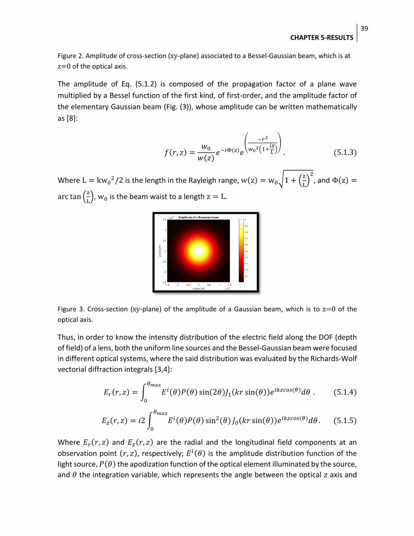
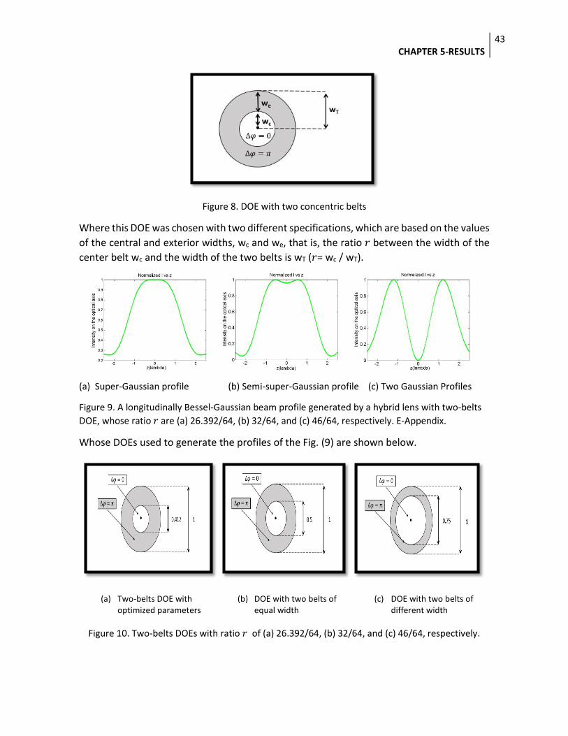
CHAPTER 5-RESULTS
37
Chapter 5
Results
------------------------------------------------------------------------------------------------------------------------
5.1. Numerical simulation
5.2. Experimental results
------------------------------------------------------------------------------------------------------------------------
5. Results
In this Section are presented the results obtained from the numerical simulation derived
from the generation of longitudinal polarized electric fields, which can be created by very
sophisticated methods, where the results have been obtained only by numerical
simulations.
5.1. Numerical simulation
A longitudinally polarized field, is a vectorial field where all the vectors associated to the
points of the field region, point at the same direction of propagation of the said field. When
this field is generated in the focal plane of an optical system, that is, within the depth of
field “DOF”, and field formed in the DOF is named focal field “FF”. Therefore, if the FF has
homogeneous intensity distributions along the DOF and subwavelength waist, then an
optical needle is obtained. Many applications have been reported about the focusing of
radially polarized vector beams to the creation of a longitudinally polarized non-diffraction
beam, that is, creating an optical needle.
Therefore, to the creation of an optical needle, firstly were simulated two light source
(Bessel-Gauss beam and an uniform line source), which have an electric field with radial
polarization, where this property of the electric field is very important for the generation of
an optical needle with longitudinal polarization, that is, longitudinally polarized non-
diffracting beam over its own extension.
Thus, the field pattern radiated (Fig. (1)) from a ULS (uniform line source) is given by [10]:
F (θ) = C sin(θ)sin [(
kL2 ) cos(θ)]
(kL2 ) cos(θ)
e θ . (5.1.1)
(The overhead equation was deducted by using physical and mathematical arguments,
which are described in the A-Appendix)
Page 52
CHAPTER 5-RESULTS
38
Where 𝐶 = −𝑖𝜔𝜇0𝐼0𝐿𝑒𝑖(𝑘𝑟−𝜔𝑡)/(4𝜋𝑟),which is normalized to 1 for convenience of
computing, 𝐿 and 𝐼0 represent the length and the constant current of the ULS, respectively,
which will be centered at the focus of the lens that focuses the field radiated and along the
optical axis of the focusing system, ω and 𝜇0 are the angular frequency and the magnetic
permeability in vacuum, respectively, 𝑘 and 𝑟 denotes the wave number and focal length of
the focusing lens, respectively, θ is the angle between the radiation direction of the SLU and
the optical axis of the focusing system, and e θ is the unit vector of the field radiated from
the ULS.
Figure 1. Cross-section of the field pattern radiated from a uniform line source of length (λ=1) in the
𝑥𝑦-plane.
In a similar way, a Bessel-Gauss beam is a possible solution in cylindrical coordinates
(𝑟, 𝜙, 𝑧) of the paraxial wave equation for an electric field with radial polarization, whose
𝜙-symmetrical amplitude (Fig. (2)) can be represented by [19]:
𝑈(𝑟, 𝑧 = 0) = 𝐴0 𝑒−
𝑟2
𝜔02𝐽0(𝛽𝑟). (5.1.2)
Where 𝐴0 is a constant parameter normalized to 1, 𝛽 is the projection of the mean wave-
vector of a Gaussian beam on the 𝑧 = 0 plane, and 𝑘 and 𝜔0 are the wavenumber and beam
waist to a length equal to the Rayleigh range, respectively.
Page 53
CHAPTER 5-RESULTS
39
Figure 2. Amplitude of cross-section (xy-plane) associated to a Bessel-Gaussian beam, which is at
z=0 of the optical axis.
The amplitude of Eq. (5.1.2) is composed of the propagation factor of a plane wave
multiplied by a Bessel function of the first kind, of first-order, and the amplitude factor of
the elementary Gaussian beam (Fig. (3)), whose amplitude can be written mathematically
as [8]:
𝑓(𝑟, 𝑧) =𝑤0
𝑤(𝑧)𝑒−𝑖Φ(𝑧)𝑒
(−𝑟2
𝑤02(1+
𝑖𝑧𝐿
))
. (5.1.3)
Where L = kw02/2 is the length in the Rayleigh range, w(z) = w0√1 + (
z
L)2
, and Φ(z) =
arc tan (z
L), w0 is the beam waist to a length z = L.
Figure 3. Cross-section (xy-plane) of the amplitude of a Gaussian beam, which is to z=0 of the
optical axis.
Thus, in order to know the intensity distribution of the electric field along the DOF (depth
of field) of a lens, both the uniform line sources and the Bessel-Gaussian beam were focused
in different optical systems, where the said distribution was evaluated by the Richards-Wolf
vectorial diffraction integrals [3,4]:
𝐸𝑟(𝑟, 𝑧) = ∫ 𝐸𝑖(𝜃)𝑃(𝜃) sin(2𝜃)𝐽1(𝑘𝑟 sin(𝜃))𝑒𝑖𝑘𝑧𝑐𝑜𝑠(𝜃)𝑑𝜃 . (5.1.4)𝜃𝑚𝑎𝑥
0
𝐸𝑧(𝑟, 𝑧) = 𝑖2∫ 𝐸𝑖(𝜃)𝑃(𝜃) sin2(𝜃) 𝐽0(𝑘𝑟 sin(𝜃))𝑒𝑖𝑘𝑧𝑐𝑜𝑠(𝜃)𝑑𝜃. (5.1.5)𝜃𝑚𝑎𝑥
0
Where 𝐸𝑟(𝑟, 𝑧) and 𝐸𝑧(𝑟, 𝑧) are the radial and the longitudinal field components at an
observation point (𝑟, 𝑧), respectively; 𝐸𝑖(𝜃) is the amplitude distribution function of the
light source, 𝑃(𝜃) the apodization function of the optical element illuminated by the source,
and 𝜃 the integration variable, which represents the angle between the optical 𝑧 axis and
Page 54
CHAPTER 5-RESULTS
40
the 𝑟 coordinate at the optical element. For both light sources, a high-NA aplanatic objective
lens is used as optical element, which has an apodization function 𝑃(𝜃) = √cos (𝜃) and a
maximum acceptance half-angle denoted as “𝜃𝑚𝑎𝑥”.
Therefore, if the radial and longitudinal field components are known, it is possible to
describe the intensity distribution and the longitudinally polarized beam profile along the
DOF, so the intensity “𝐼” at each observation point (𝑟, 𝑧) can be calculated by:
𝐼 = |𝐸𝑟(𝑟, 𝑧)|2 + |𝐸𝑧(𝑟, 𝑧)|
2 . (5.1.6)
Consequently, for the first light source (uniform linear source, ULS), the electric field pattern
is radiated in a 4pi focused system, which is composed of two aplanatic objective lenses,
each with NA=1. In order to obtain a longitudinally polarized beam, the electric field pattern
is radiated and focused with a phase difference of 180 degrees (∆𝜑 = 𝜋) between the
electric fields, that is, the 4pi system is illuminated by two counter-propagating radially
polarized beams with a relative π phase shift. Thus, under these conditions the
longitudinally polarized beam profile Fig. (4) is flat over most of the covered area with
intensity, that is, a flat-top longitudinally polarized beam; this beam is not diffracted along
a distance, that is, it is a non-diffracting beam on its own extent or FWHM (full width at half
maximum), where this represents the optical needle length, which depends of the size L of
the uniform linear source.
(a) Flat-top beam with 3.25λ FWHM (b) Flat-top beam with 5.25 λ FWHM
(c) Flat-top beam with 7.23λ FWHM (d) Flat-top beam with 9.24λ FWHM
Page 55
CHAPTER 5-RESULTS
41
Figure 4. Flat-top beams with specific FWHM generated by a uniform linear source with
length (a) 4λ, (b) 6λ, (c) 8λ, and (d) 10λ, respectively. B-Appendix.
Other important parameter associated to the optical needle, is its diameter, that is, the
longitudinally polarized beam waist , which has a sub-wavelength size Fig. (5) and it does
not change along the FWHM of the flat-top beam, where its waist 𝑤 does not depend on
the size L of the ULS.
a) Optical needle with 3.25λ FWHM b) Optical needle with 5.25λ FWHM
…..
c) Optical needle with 7.23λ FWHM d) Optical needle with 9.24λ FWHM
Figure 5. Different FWHM and equal waist (0.36λ) optical needles, which are generated by
a) 4λ-, b) 6λ-, c) 8λ and d) 10λ-length uniform linear sources, respectively. C-Appendix.
Similarly, the second light source (a Bessel-Gaussian beam with radial polarization), it is
focused in an aplanatic objective lens with a NA=0.95 to obtain a longitudinally polarized
beam with Gaussian profile Fig. 6(a), and in order to achieve a longitudinally polarized beam
with flat profile Fig. 6(b), was added a DOE (Diffractive Optical Element) with five concentric
belts.
Page 56
CHAPTER 5-RESULTS
42
(a) Gaussian profile (b) Super-Gaussian profile (c) Two semi-Gaussian Profiles
Figure 6. A longitudinally polarized beam profile generated by (a) an aplanatic lens, (b) a hybrid
lens with five equally spaced belts, and (c) a hybrid lens with five differently spaced belts,
respectively. D-Appendix.
Where these DOEs are simulated both with equal and different spacing between each belt
Fig. 7(a) and Fig. 7(b), respectively, and whose phase shift ∆𝜑 between a belt and another
of 0 and 𝜋 radians, respectively; which means that the radially polarized Bessel-Gaussian
beam firstly impinge on the DOE and then it is focused by the aplanatic lens, where to the
set of a lens with a DOE, it will be called “hybrid lens”.
(a) DOE with five equally spaced belts (b) DOE with five differently spaced belts
Figure 7. DOE with equal and different spacing between each belts, whose relative
diameters of each belt are (a) 0.2, 0.4, 0.6, 0.8 and 1, and (b) 0.091, 0.391, 0.592, 0.768 and
1, respectively.
Fig. (8) shows the geometry associated to a DOE with two concentric belts and fig. (9) shows
the profiles generated numerically using an aplanatic lens with NA=0.95
Page 57
CHAPTER 5-RESULTS
43
Figure 8. DOE with two concentric belts
Where this DOE was chosen with two different specifications, which are based on the values
of the central and exterior widths, wc and we, that is, the ratio 𝑟 between the width of the
center belt wc and the width of the two belts is wT (𝑟= wc / wT).
(a) Super-Gaussian profile (b) Semi-super-Gaussian profile (c) Two Gaussian Profiles
Figure 9. A longitudinally Bessel-Gaussian beam profile generated by a hybrid lens with two-belts
DOE, whose ratio 𝑟 are (a) 26.392/64, (b) 32/64, and (c) 46/64, respectively. E-Appendix.
Whose DOEs used to generate the profiles of the Fig. (9) are shown below.
(a) Two-belts DOE with optimized parameters
(b) DOE with two belts of equal width
(c) DOE with two belts of different width
Figure 10. Two-belts DOEs with ratio 𝑟 of (a) 26.392/64, (b) 32/64, and (c) 46/64, respectively.
Page 58
CHAPTER 5-RESULTS
44
Thus, when the five-belts-DOE have a different spacing between each belt, the
longitudinally polarized beam profile will be flat over most of the covered area with
intensity and at the same time, the beam will be non-diffractive along a distance, that is,
along its own FWHM (4λ) and it represents the optical needle length, which depends of the
spacing between each belt of the DOE.
Therefore, when the beam is non-diffractive, it propagates without divergence over its
FWHM, implying that the beam will have a constant waist, which is of sub-wavelength size;
on the other hand, the FWHM and the beam waist are parameters that depend of the
characteristics of the DOE, that is, of its belts number and spacing between each one.
(a) Optical needle generated by only an aplanatic lens
(b) Optical needle generated by hybrid
lens with five differently spaced
belts
(c) Optical needles generated by
hybrid lens with five equally
spaced belts
Figure 11. Beams with FWHM of (a) 1.4λ and variable waist (b) 4.4λ and 0.44 λ constant waist, and (c) 1.67λ
and variable waist (both), respectively (the mentioned waists are taken with respect to their own FWHM). F-
Appendix.
Page 59
CHAPTER 5-RESULTS
45
(a) Optical needle generated by hybrid lens with two belts and 𝑟=26.392/64
(b) Optical needle generated by
hybrid lens with two equally
spaced belts
(c) Optical needle generated by
hybrid lens with two belts and
𝑟=46/64
Figure 12. Beams with FWHM of (a) 2.5λ and 0.74 λ constant waist, (b) 2.72λ and variable waist, and (c)
1.75λ and variable waist (both, respectively (The mentioned waists are taken with respect to their own
FWHM). G-Appendix.
Thus, If one uses an aplanatic NA=0.95 lens with either a two-belts DOE or five-belts DOE,
can be generated linearly polarized subwavelength non-diffracting beams (optical needle
with longitudinal polarization) along the z-axis (optical needle) or beams without divergence
(constant waist) over its own FWHM (optical needle length). However, when one change
the NA (Numerical Aperture) of the aplanatic lens, this generates a longitudinally polarized
beams with different parameters, that is, waist and FWHM with different measurements,
where both increase if the NA decreases, and in the same way, if the NA increases, both the
waist and FWHM decrease.
Page 60
CHAPTER 5-RESULTS
46
Therefore, three longitudinally polarized beams generated by using an aplanatic lens of
NA=0.90, NA=0.95 and NA=0.975 were simulated, which are shown in the following fig. (13).
(a)
(b) (c)
Figure 13. Longitudinally polarized beams generated by an aplanatic lens of (a) NA=0.90, (b)
NA=0.95, and (c) NA=0.975, respectively. H-Appendix.
Similarly, if now one has an aplanatic lens of NA=0.90 and are further added individually the
DOEs that are shown in the fig. (10), one can see that as in the fig. (12), the generated
longitudinally polarized beam are shown in the figure 14, which increases its parameters
(waist and FWHM) without changing its shape in comparison with the beams shown in the
fig. (12), which are generated by the same DOE and an aplanatic lens of higher numerical
aperture (NA=0.95).
Page 61
CHAPTER 5-RESULTS
47
(a) (b)
,,,,,,,,,,,
(c) (d)
(e) (f)
Figure 14. Longitudinally polarized beams generated by using an aplanatic lens and a DOE, both with
different parameters, that is, widths ratio and numerical aperture of (a) 𝑟=26.392/64 and NA=0.90,
(b) 𝑟=26.392/64 and NA=0.95, (c) 𝑟=32/64 and NA=0.90, (d) 𝑟=32/64 and NA=0.95, (e) 𝑟=46/64 and
NA=0.90, (f) 𝑟=46/64 and NA=0.95, respectively. G-Appendix.
Page 62
CHAPTER 5-RESULTS
48
5.2. Experimental results
To the best of our knowledge, there exist a lack of reported results describing the
experimental verification of several of the methods for generating specific focal fields,
which are revised in this work. Therefore, an experimental method for verifying the
existence of such beams is proposed here, which could prove the results obtained by
numerical simulations, in this case the beams shown in the Fig. 14(c) and Fig. 14(e).
Let us consider beams are achieved by a beam with radial polarization, which are generated
by using a polarization converter, and this is a commercial device named S-WP (S-
Waveplate). Then, the radially polarized beam is transmitted through a specific parameters
manufactured DOE (the designed and used DOEs are shown in the I-Appendix). The beam
after the DOE is focused in an aplanatic MO (microscope objective) of NA=0.90 (see fig.
(15)).
Figure 15. Optical arrangement proposed to be used in the laboratory.
Thus, when one has the radially polarized beam transmitted through a DOE, a longitudinally
polarized beam is originated at the deep of focus region (DOF). Here we propose that the
intensity distribution can be verified by using a vision system, which consists of a CMOS
camera and an image forming lens, which are set over a translation stage to a fixed distance
di, according to fig. (16).
Figure 16. Vision system for the detection of a focal field
Page 63
CHAPTER 5-RESULTS
49
Thus, this system can be displaced along the z-axis in order to verify the focal field formed
in the DOF. This field can be scanned registering the images of the object that is located at
the distance 𝑑𝑜 at different positions, given by equally spaced ∆z steps of the translation
stage, whose object position can be calculated by means of the Gauss’ law, which can be
represented as:
𝑑𝑜 =𝑓2𝑑𝑖
𝑑𝑖 − 𝑓2. (5.2.1)
Where 𝑑𝑜 is the distance between the focal plane of the MO and the image forming lens, di
is the fixed distance between the image forming lens and the CMOS camera sensor, and f2
is the focal length of the image forming lens.
On the other hand, an important consideration in this proposed method is that the focal
field should be registered, while the ∆z steps of the translation stage are less than the
FWHM of the longitudinal polarized beam formed in the DOF.
Page 64
CHAPTER 6-CONCLUTIONS
50
Chapter 6
Conclusions
------------------------------------------------------------------------------------------------------------------------
------------------------------------------------------------------------------------------------------------------------
6. Conclusions
The polarization is an important tool in optics and engineering, where many applications
have reported focusing radially polarized vector-beams for generating longitudinally
polarized beams, which can be obtained by using a lenses system of high NA (numerical
aperture) or mirrors with very specific design. On the other hand, if one wants to get a non-
diffracting longitudinal polarized beam with long FWHM (full width at half maximum) and
subwavelength waist, that is, an ultra-long optical needle, one can use complementarily a
diffractive optical element with concentric rings, where depending on the number of belts,
the spacing between them and phase shift in each ring, will be the beam intensity profile,
or in some cases, it is only change the size of the light source; similarly, if one wants to have
additionally a beam with ultra-small (subwavelength) waist size, one can change the value
of the NA of the used focusing lenses system, that is, if the value of the NA increases, the
size of the beam waist decreases. However, not only decreases the size of the beam waist,
but also its FWHM and consequently there will be a decrease of the zone to study and
analyze with these beams, in this case, a decrease of the DOF (depth of field) of the used
optical system.
Therefore, when a want to generate along the DOF an ultra-long optical needle with ultra-
small waist, that is, a non-diffracting beam with high beam quality and subwavelength
waist, one has to use a specific combination of different optical elements and an
appropriate light source, where the parameters of these elements should be selected
properly, since there is not a total dependence between these parameters and then is not
possible to optimize at the same time all the beam parameters.
Page 65
APPENDIX
51
Appendix A. Deduction of the field pattern radiated from a ULS
Given that a uniform linear source is a thin wire of 𝐿 length that is aligned along the optical
z axis, and whose electric current distribution within the wire is 𝐼 = 𝐼0𝑒𝑖(𝑘𝑅−𝜔𝑡) Fig. (1).
One can know the induction of magnetic field and by using the Ampere’s law then know the
electric field pattern radiated by the wire.
Figure 1. Radiation pattern by a thin wire of 𝐿 length
Thus, in order to know �� , the Biot-Savart was used, which can be written as:
�� (𝑟 ) = ∇ × [𝜇0
4𝜋∮
𝐼(𝑟 ′)𝑑𝑟 ′
𝑅
𝐿/2
−𝐿/2 ]. (1)
Where 𝑟 ′ is the direction vector of the electric current, 𝑟 is the vector from the wire to the
observation point and 𝑅 is ‖𝑟 − 𝑟 ′‖.
If 𝑟 ′ = 𝑧��𝑧 and 𝑟 = 𝑥��𝑥 + 𝑦��𝑦 + 𝑧��𝑧, 𝑅 = √𝑟2 + 𝑧2 − 2𝑧𝑟𝑐𝑜𝑠(𝜃), and since the radiated
field pattern is observed away from the wire, 𝑟 > 𝑧 and then 𝑅 ≈ 𝑟√1 − 2𝑐𝑜𝑠(𝜃) (𝑧
𝑟).
Similarly, as 𝑧/𝑟 is a very small number, it is possible to approximate 𝑅 to two terms of the
Taylor series of √1 − 𝑥 and consequently 𝑅 ≈ 𝑟 − 𝑧𝑐𝑜𝑠(𝜃).
Therefore, the Eq. (1) can be rewritten as:
�� (𝑟 ) = ∇ × [𝜇0
4𝜋∮
𝐼0𝑒𝑖(𝑘𝑅−𝜔𝑡)𝑑𝑧
𝑟
𝐿/2
−𝐿/2 ��𝑧]. (2)
Accordingly, first the 𝐴 potential inside the square brackets of the Eq. (1) will calculated, so
that �� (𝑟 ) can be expressed as:
Page 66
APPENDIX
52
�� (𝑟 ) = ∇ × [𝐴𝑧��𝑧]. (3)
With 𝐴𝑧 =𝜇0𝐼0𝐿
4𝜋
𝑒𝑖(𝑘𝑟−𝜔𝑡)
𝑟
𝑠𝑖𝑛[𝑘𝐿
2cos (𝜃)]
[𝑘𝐿
2cos (𝜃)]
.
In order to simplify and then solver the Eq. (3), 𝐴 is written in spherical coordinates as shown
below:
𝐴 = 𝐴𝑧 cos(𝜃) ��𝑟 − 𝐴𝑧 sin(𝜃) ��𝜃. (4)
Thus, when ∇ × 𝐴 is calculated, the �� (𝑟 ) can be rewritten as:
�� (𝑟 ) =1
𝑟{
𝜕
𝜕𝑟[𝑟 (−
𝜇0𝐼0𝐿𝑒−𝑖𝜔𝑡
4𝜋
𝑒𝑖𝑘𝑟
𝑟 𝑠𝑖𝑛[
𝑘𝐿
2cos(𝜃)]
[𝑘𝐿
2cos(𝜃)]
) sin (𝜃)]
−𝜕
𝜕𝜃[(
𝜇0𝐼0𝐿𝑒−𝑖𝜔𝑡
4𝜋
𝑒𝑖𝑘𝑟
𝑟
𝑠𝑖𝑛[𝑘𝐿
2cos(𝜃)]
[𝑘𝐿
2cos(𝜃)]
) cos(𝜃)]} ��𝜑 . (5)
In the same way, since 1/𝑟2 is a very small number, the second term of the Eq. (5) can be
neglected, so �� (𝑟 ) can be rewritten as:
�� (𝑟 ) = −𝑖𝑘
𝑟
𝜇0𝐼0𝐿
4𝜋𝑒𝑖(𝑘𝑟−𝜔𝑡) sin(𝜃)
𝑠𝑖𝑛[𝑘𝐿
2cos(𝜃)]
[𝑘𝐿
2cos(𝜃)]
��𝜑. (6)
Therefore, in order to know �� (𝑟 ), the Ampere’s law (∇ × �� = 𝜇0휀0𝜕��
𝜕𝑡) is used, where first
∇ × �� (𝑟 ), which can be written as:
∇ × �� (𝑟 ) = −𝜇0𝐼0𝐿𝑘2
4𝜋𝑟𝑒𝑖(𝑘𝑟−𝜔𝑡)sin(𝜃)
𝑠𝑖𝑛[𝑘𝐿
2cos(𝜃)]
[𝑘𝐿
2cos(𝜃)]
��𝜃. (7)
Finally, If ∇ × �� (𝑟 ) is known, �� (𝑟 ) = 𝑐2 ∫∇ × �� (𝑟 ) 𝑑𝑡 ��𝜃, which can be written as:
�� (𝑟 ) = −𝑖𝜇0𝐼0𝐿𝜔
4𝜋𝑟𝑒𝑖(𝑘𝑟−𝜔𝑡) 𝑠𝑖𝑛(𝜃)
𝑠𝑖𝑛[(𝑘𝐿
2) 𝑐𝑜𝑠(𝜃)]
(𝑘𝐿
2) 𝑐𝑜𝑠(𝜃)
��𝜃 . (8)
B. FWHM of a flat-top beam %%% Length of the optical needle
clc
close all
%% parameters
l=1;%lambda
A=1;
k=2*pi/l;
n=10;%length of the uniform linear source
L=n*l;
c=1;
Page 67
APPENDIX
53
r=0; % r coordinate
angle=90;
t=linspace(0,angle*pi/180,1000);
IEZI=0;
for z=-6:0.01:6;
a=( (c.*sin(t).*sin((k*L/2).*cos(t))./((k*L/2).*cos(t)))
.* ((cos(0)).^(1/2))...
.* (sin(t).^2) .* (besselj(0,k* (r) .*sin(t))) .*
(exp(1i*k*z.*cos(t))) ) ;
ez=trapz(t,a);
EZ=2*A*1i*ez;
IEZI=[IEZI, (imag(EZ))^2];
end
z=-6:0.01:6;
figure(1);
%% beam profile
plot(z,IEZI(2:end),'r.');
%% normalized beam profile
IEZIM=max(max(IEZI));
IN=IEZI/IEZIM;
figure(2);
plot(z,IN(2:end),'g.');
title('Normalized I vs z')
xlabel('z(lambda)')
ylabel('Intensity on the optical axis')
hold on;
drawnow
C. Waist of a non-diffracting beam %%% Optical needle with an ULS
%%
clear,clc,close all,
%% Main parameters
l=1; % wavelength
A=1; % constant amplitude
k=2*pi/l; % wavenuber
n=10; % length parameter of the uniform line source
L=n*l; % length of uniform line source
Page 68
APPENDIX
54
c=1; % constant related to the uniform line source
strength
%% integration variable t for the integral (trapz)
t=linspace(0,90*pi/180,1000);
I=zeros(1,1201);
for r=-1:0.01:1
Iz=0;
Ir=0;
for z=-6:0.01:6;
F=c.*sin(t).*sin((k*L/2).*cos(t))./((k*L/2).*cos(t));
ar=( ( F ) ...
.* (sin(2*t)/2) .* (besselj(1,k* (r) .*sin(t))) .*
(exp(1i*k*z.*cos(t))) ) ;
er=trapz(t,ar);
ER=2*A*er;
Ir=[Ir real(abs(ER).^2)];
az=( ( F ) ...
.* (sin(t).^2) .* (besselj(0,k* (r) .*sin(t))) .*
(exp(1i*k*z.*cos(t))) ) ;
ez=trapz(t,az);
EZ=2*A*1i*ez;
Iz=[Iz imag(EZ)^2];
end
Iz=Iz(2:end);
Ir=Ir(2:end);
I=[I;Iz+Ir];
z=-6:0.01:6;
end
I=I(2:end,:);
r=-1:0.1:1; % invert axis
figure(1)
imagesc(z,r,I),colormap hot;
title('r-z Plane vs I ')
xlabel('z(lambda)')
ylabel('r(lambda)')
D. Length of the optical needle for the BG beam and by using a DOE with five-belts
%% Length of the optical needle for the BG beam
clc
close all
%% parameters
l=1;%lambda
Page 69
APPENDIX
55
A=1;
k=2*pi/l;
r=0; % r coordinate
angle=asin(0.95); % acceptance angle and numerical aperture
t=linspace(0,angle,1000);
IEZI=0;
%%
for z=-2.50:0.01:2.50;
beta=1;
gamma=1;
BG=exp( -(beta^2) * (sin(t)/sin(asin(angle))).^2 )
.* ...
besselj(1,2*gamma*(sin(t)/sin(asin(angle))));
%% with five optimized belts
% interval1=t>=0 & t<4.96*pi/180; %r1
% interval2=t>=21.79*pi/180 & t<34.25*pi/180; %r3
% interval3=t>=46.87*pi/180 & t<=asin(angle); %r5
% maskPositive=interval1 + interval2 + interval3;
% maskNegative=~maskPositive;
% T=maskPositive-maskNegative;
%% with five equally spaced belts
% interval1=t>=0 & t<angle/5; %r1
% interval2=t>=angle*2/5 & t<angle*3/5; %r3
% interval3=t>=angle*4/5 & t<=angle; %r5
% maskPositive=interval1 + interval2 + interval3;
% maskNegative=~maskPositive;
% T=maskPositive-maskNegative;
%% without DOE
% T=1 ;
%% evaluation of the integral
a=( ( T.* BG ) .* ((cos(t)).^(1/2))...
.* (sin(t).^2) .* (besselj(0,k* (r) .*sin(t))) .*
(exp(1i*k*z.*cos(t))) ) ;
ez=trapz(t,a);
Page 70
APPENDIX
56
EZ=2*A*1i*ez;
IEZI=[IEZI, real(abs(EZ).^2)];
end
%%
z=-2.50:0.01:2.50;
figure(1);
%% beam profile
plot(z,IEZI(2:end),'r.');
%% normalized beam profile
IEZIM=max(max(IEZI));
IN=IEZI/IEZIM;
figure(2);
plot(z,IN(2:end),'g.');
title('Normalized I vs z')
xlabel('z(lambda)')
ylabel('Intensity on the optical axis')
hold on;
drawnow
E. Length of the optical needle for the BG beam and by using a DOE with two-belts
%% Length of the optical needle for the BG beam
clc
close all
%% parameters
l=1;%lambda
A=1;
k=2*pi/l;
r=0; % r coordinate
angle=asin(0.95); % acceptance angle and numerical aperture
t=linspace(0,angle,1000);
IEZI=0;
%%
for z=-2.50:0.01:2.50;
beta=1;
gamma=1;
BG=exp( -(beta^2) * (sin(t)/sin(asin(angle))).^2 )
.* ...
Page 71
APPENDIX
57
besselj(1,2*gamma*(sin(t)/sin(asin(angle))));
%% with five optimized belts
% interval1=t>=0 & t<4.96*pi/180; %r1
% interval2=t>=21.79*pi/180 & t<34.25*pi/180; %r3
% interval3=t>=46.87*pi/180 & t<=asin(angle); %r5
% maskPositive=interval1 + interval2 + interval3;
% maskNegative=~maskPositive;
% T=maskPositive-maskNegative;
%% with five equally spaced belts
% interval1=t>=0 & t<angle/5; %r1
% interval2=t>=angle*2/5 & t<angle*3/5; %r3
% interval3=t>=angle*4/5 & t<=angle; %r5
% maskPositive=interval1 + interval2 + interval3;
% maskNegative=~maskPositive;
% T=maskPositive-maskNegative;
%% without DOE
% T=1 ;
%% evaluation of the integral
a=( ( T.* BG ) .* ((cos(t)).^(1/2))...
.* (sin(t).^2) .* (besselj(0,k* (r) .*sin(t))) .*
(exp(1i*k*z.*cos(t))) ) ;
ez=trapz(t,a);
EZ=2*A*1i*ez;
IEZI=[IEZI, real(abs(EZ).^2)];
end
%%
z=-2.50:0.01:2.50;
figure(1);
%% beam profile
plot(z,IEZI(2:end),'r.');
%% normalized beam profile
IEZIM=max(max(IEZI));
IN=IEZI/IEZIM;
figure(2);
Page 72
APPENDIX
58
plot(z,IN(2:end),'g.');
title('Normalized I vs z')
xlabel('z(lambda)')
ylabel('Intensity on the optical axis')
hold on;
drawnow
F. Optical needle by using a five-belts DOE %% OPTICAL NEEDLE WITH A B-G BEAM
tic %(initial time)
close all
l=1; % wavelength
A=1; % amplitude constant
k=2*pi/l; % wavenuber
% n=10; % length parameter of uniform line source
% L=n*l; % length of uniform line source
c=1; % constant related to the uniform line source
strength
alfa=0.95; % NA
t=linspace(0,asin(alfa),1000);
i_s=6; % image size
I=zeros(1, 200*i_s + 1 );
for r=-2.5:0.01:2.5;
Iz=0;
Ir=0;
for z=-1*i_s:0.01:i_s;
%% light source
beta=1;
gamma=1;
BG=exp( -(beta^2) * (sin(t)/sin(asin(alfa))).^2 )
.* ...
besselj(1,2*gamma*(sin(t)/sin(asin(alfa))));
% % % parameters of the DOE
% % five belts with optimazed parameters
% interval1=t>=0 & t<4.96*pi/180; %r1
% interval2=t>=21.79*pi/180 & t<34.25*pi/180; %r3
% interval3=t>=46.87*pi/180 & t<=asin(alfa); %r5
% maskPositive=interval1 + interval2 + interval3;
Page 73
APPENDIX
59
% maskNegative=~maskPositive;
% T=maskPositive-maskNegative;
% % five equally spaced belts
% interval1=t>=0 & t<asin(alfa)/5; %r1
% interval2=t>=asin(alfa)*2/5 & t<asin(alfa)*3/5; %r3
% interval3=t>=asin(alfa)*4/5 & t<=asin(alfa); %r5
% maskPositive=interval1 + interval2 + interval3;
% maskNegative=~maskPositive;
% T=maskPositive-maskNegative;
% % % without DOE
T=1;
%% Richard-Wolf vectorial diffraction integral
ar=( T.* ( BG ) ...
.* (sin(2*t)/2) .* (besselj(1,k* (r) .*sin(t))) .*
(exp(1i*k*z.*cos(t))) ) ;
er=trapz(t,ar);
ER=2*A*er;
Ir=[Ir real(abs(ER).^2)];
az=( T.* ( BG ) ...
.* (sin(t).^2) .* (besselj(0,k* (r) .*sin(t))) .*
(exp(1i*k*z.*cos(t))) ) ;
ez=trapz(t,az);
EZ=2*A*1i*ez;
Iz=[Iz real(abs(EZ).^2)]; % imag(EZ)^2
end
Iz=Iz(2:end);
Ir=Ir(2:end);
I=[I;Iz+Ir];
z=-1*i_s:0.01:i_s;
end
I=I(2:end,:)/max(max( I(2:end,:) ));
r=-2.5:0.1:2.5;
figure(2)
imagesc(z,r,I),colormap jet;colorbar;
title('r-z Plane vs I ')
xlabel('z(lambda)')
ylabel('r(lambda)')
axis 'square'
toc % (final time)
Page 74
APPENDIX
60
G. Optical needle by using a two-belts DOE
%% OPTICAL NEEDLE WITH A B-G BEAM
tic %(initial time)
close all
l=1; % longitud de onda
A=1; % amplitude constant
k=2*pi/l; % wavenuber
% n=10; % length parameter of uniform line source
% L=n*l; % length of uniform line source
c=1; % constant related to the uniform line source
strength
alfa=0.95; % NA
t=linspace(0,asin(alfa),1000);
i_s=2.5; % image size
I=zeros(1, 200*i_s + 1 );
for r=-2.5:0.01:2.5;
Iz=0;
Ir=0;
for z=-1*i_s:0.01:i_s;
%% light source
beta=1;
gamma=1;
BG=exp( -(beta^2) * (sin(t)/sin(asin(alfa))).^2 )
.* ...
besselj(1,2*gamma*(sin(t)/sin(asin(alfa))));
% % % parameters of the DOE
% % two equally spaced belts with ratio 1/2 a 1/2
% interval1=t>=0 & t<asin(alfa)/2; %r1
% % interval2=t>=asin(alfa)*2/5 & t<asin(alfa)*3/5;
%r3
% % interval3=t>=asin(alfa)*4/5 & t<=asin(alfa); %r5
% maskPositive=interval1
% maskNegative=~maskPositive;
% T=maskPositive-maskNegative;
% % two belts with variable r (radius)
% radius=26.392;
Page 75
APPENDIX
61
% % 2 BELTS WITH RATIO OF RADIUS/64 TO (RADIUS-64)/64.
% interval1=t>=0 & t<asin(alfa)*radius/64; %r1
% % interval2=t>=asin(alfa)*2/5 & t<asin(alfa)*3/5;
%r3
% % interval3=t>=asin(alfa)*4/5 & t<=asin(alfa); %r5
% maskPositive=interval1
% maskNegative=~maskPositive;
% T=maskPositive-maskNegative;
% % % without DOE
T=1;
%% Richard-Wolf vectorial diffraction integral
ar=( T.* ( BG ) ...
.* (sin(2*t)/2) .* (besselj(1,k* (r) .*sin(t))) .*
(exp(1i*k*z.*cos(t))) ) ;
er=trapz(t,ar);
ER=2*A*er;
Ir=[Ir real(abs(ER).^2)];
az=( T.* ( BG ) ...
.* (sin(t).^2) .* (besselj(0,k* (r) .*sin(t))) .*
(exp(1i*k*z.*cos(t))) ) ;
ez=trapz(t,az);
EZ=2*A*1i*ez;
Iz=[Iz real(abs(EZ).^2)]; % imag(EZ)^2
end
Iz=Iz(2:end);
Ir=Ir(2:end);
I=[I;Iz+Ir];
z=-1*i_s:0.01:i_s;
end
I=I(2:end,:)/max(max( I(2:end,:) ));
r=-2.5:0.1:2.5;
figure(2)
imagesc(z,r,I),colormap jet;colorbar;
title('r-z Plane vs I ')
xlabel('z(lambda)')
ylabel('r(lambda)')
axis 'square'
toc % (final time)
H. Longitudinally polarized beam with variable NA
Page 76
APPENDIX
62
%% OPTICAL NEEDLE WITH A B-G BEAM
tic %(initial time)
close all
l=1; % longitud de onda
A=1; % amplitude constant
k=2*pi/l; % wavenuber
% n=10; % length parameter of uniform line source
% L=n*l; % length of uniform line source
c=1; % constant related to the uniform line source
strength
alfa=0.95; % NA
t=linspace(0,asin(alfa),1000);
i_s=2.5; % image size
I=zeros(1, 200*i_s + 1 );
for r=-2.5:0.01:2.5;
Iz=0;
Ir=0;
for z=-1*i_s:0.01:i_s;
%% light source
beta=1;
gamma=1;
BG=exp( -(beta^2) * (sin(t)/sin(asin(alfa))).^2 )
.* ...
besselj(1,2*gamma*(sin(t)/sin(asin(alfa))));
%% Richard-Wolf vectorial diffraction integral
ar=( 1.* ( BG ) ...
.* (sin(2*t)/2) .* (besselj(1,k* (r) .*sin(t))) .*
(exp(1i*k*z.*cos(t))) ) ;
er=trapz(t,ar);
ER=2*A*er;
Ir=[Ir real(abs(ER).^2)];
az=( T.* ( BG ) ...
.* (sin(t).^2) .* (besselj(0,k* (r) .*sin(t))) .*
(exp(1i*k*z.*cos(t))) ) ;
ez=trapz(t,az);
EZ=2*A*1i*ez;
Iz=[Iz real(abs(EZ).^2)]; % imag(EZ)^2
end
Iz=Iz(2:end);
Ir=Ir(2:end);
I=[I;Iz+Ir];
z=-1*i_s:0.01:i_s;
Page 77
APPENDIX
63
end
I=I(2:end,:)/max(max( I(2:end,:) ));
r=-2.5:0.1:2.5;
figure(2)
imagesc(z,r,I),colormap jet;colorbar;
title('r-z Plane vs I ')
xlabel('z(lambda)')
ylabel('r(lambda)')
axis 'square'
toc % (final time)
I. Two-belts DOEs Designs
Figure 1. Two-belts DOE with ratio 𝑟 of 32/64
Page 78
APPENDIX
64
Figure 2. Two-belts DOE with ratio 𝑟 of 46/64
Page 79
BIBLIOGRAPHY
65
Bibliography
1. H. F. Wang, L. P. Shi, B. Lukyanchuk, C. Sheppard, and C. T. Chong, “Creation of a
needle of longitudinally polarized light in vacuum using binary optics,” Nat. Photonics 2(8), 501–505 (2008).
2. Y. Yu and Q. Zhan, “Optimization-free optical focal field engineering through reversing the radiation pattern from a uniform line source,” Opt. Express. 23(6), 7527-7534 (2015)
3. E. Wolf, “Electromagnetic diffraction in optical systems I. An integral representation of the image field,” Proc. R. Soc. Ser. A 253, 349–357 (1959).
4. B. Richards and E. Wolf, “Electromagnetic diffraction in optical system II. Structure of the image field in an aplanatic system,” Proc. R. Soc. Ser. A 253, 358–379 (1959).
5. K. Huang, P. Shi, X. L. Kang, X. B. Zhang, and Y. P. Li, “Design of DOE for generating a needle of a strong longitudinally polarized field,” Opt. Lett. 35(7), 965–967 (2010).
6. N. Bokor and N. Davidson, “Toward a spherical spot distribution with 4pi focusing of radially polarized light,” Opt. Lett. 29(17), 1968–1970 (2004).
7. S. Yan, B. Yao, and R. Rupp, “Shifting the spherical focus of a 4Pi focusing system,” Opt. Express 19(2), 673–678 (2011).
8. D. G. Hall, “Vector-beam solutions of Maxwell’s wave equation”, Opt. Lett. 21, 9-11 (1996).
9. K. S. Youngworth and T. G. Brown, “Focusing of high numerical aperture cylindrical-vector beams,” Opt. Express 7(2), 77–87 (2000).
10. W. L. Stutzman and G. A. Thiele, Antenna Theory and Design, 2nd Edition (J. Wiley, 1998).
11. J. Liu, M. Ai, J. Tan, R. Wang, and X. Tan, “Focusing of cylindrical-vector beams in elliptical mirror based system with high numerical aperture,” Opt. Commun, 305, 71–75 (2013).
12. M. Lieb and A.Meixner, “A high numerical aperture parabolic mirror as imaging device for confocal microscopy,” Opt. Express 8(7), 458–474 (2001).
13. H. Dehez, A. April, and M. Piche, “Needles of longitudinally polarized light: guidelines for minimum spot size and tunable axial extent,” Opt. Express 20(14), 14891–14905 (2012).
14. T. Liu, J. Tan, J. Lin, and J. Liu, “Generating super-Gaussian light needle of 0.36λ beam size and pure longitudinal polarization,” Opt. Eng. 52(7), 074104 (2013).
15. J. Lin et al., “Achievement of longitudinally polarized focusing with long focal depth by amplitude modulation,” Opt. Lett. 36(7), 1185–1187 (2011).
16. W. Chen and Q. Zhan, “Creating a spherical focal spot with spatially modulated radial polarization in 4Pi microscopy,” Opt. Lett. 34(16), 2444–2446 (2009).
17. J. Wang, W. Chen, and Q. Zhan, “Three-dimensional focus engineering using dipole array radiation pattern”, Opt. Commun. 284(12), 2668–2671 (2011).
18. A. Ashikin and J. Z. Dziedzic, “Optical trapping and manipulation of viruses and bacteria” Science. 235, 1517-1520 (1987).
Page 80
BIBLIOGRAPHY
66
19. Q. Zhan, “Cylindrical vector beams: from mathematical concepts to applications,” Adv. Opt. Photon 1(1), 1–57 (2009).
20. S. Bravo Yuste, Métodos matemáticos avanzados para científicos e ingenieros, Edición electrónica: Pedro Cid, S.A. (Universidad de Extremadura. Servicio de Publicaciones, 2006).