Page 1
ENSC 427: COMMUNICATION NETWORKS
ANALYSIS ON VOIP USING OPNET
FINAL PROJECT
Benson Lam 301005441 [email protected]
Winfield Zhao 200138485 [email protected]
Mincong Luo 301039612 [email protected]
Data: April 05, 2009
http://www.sfu.ca/~btl2/web.html
Page 2
II
ABSTRACT
VoIP is a technology that permits communication calls to be made over the internet and it
is expected to become the mainstream for communication due to its low cost. However,
the quality of VoIP is mainly impaired by jitter, delay, packet loss and many other
parameters. As a case study, we simulate a VoIP network and study the behaviour and
quality of VoIP under different scenarios. Furthermore, we study all the potential
parameters that can deteriorate the quality of VoIP. This document presents an
informative description of our VoIP network and discusses many design and technical
issues pertaining to the deployment of VoIP.
Page 3
III
TABLE OF CONTENT
Abstract..............................................................................................................................................II
Table of Content ................................................................................................................................ III
List of Figures....................................................................................................................................V
List of Tables................................................................................................................................... VII
1 Introduction .................................................................................................................................... 1
1.1 What is VoIP ........................................................................................................................... 1
1.2 VoIP Deterioration Factors........................................................................................................ 1
1.2.1 Jitter................................................................................................................................. 2
1.2.2 End-to-End Delay.............................................................................................................. 2
1.2.3 Packet Loss....................................................................................................................... 2
1.2.4 Internet Qos and Coding scheme......................................................................................... 3
2 Project Description .......................................................................................................................... 3
3 Simulation Approach ....................................................................................................................... 5
4 Setting VoIP Application ................................................................................................................. 7
5 Conversation Pair ............................................................................................................................ 9
6 Discussion .................................................................................................................................... 11
6.1 Scenario one: ......................................................................................................................... 12
Comparison between Local and Long-distance VoIP Communication .............................................. 12
6.2 Scenario Two: ........................................................................................................................ 16
Comparison between a Busy Network and a Non-busy VoIP Network ............................................. 16
6.3 Scenario Three: ...................................................................................................................... 21
Observation of VoIP Quality under Different Discard Ratio (Internet QoS) ...................................... 21
6.4 Scenario Four:........................................................................................................................ 25
Different Encoder Schemes Usage and Their Effects on VoIP Quality.............................................. 25
7 Conclusion.................................................................................................................................... 27
Page 4
IV
8 Reference...................................................................................................................................... 28
9 Appendix I.................................................................................................................................... 30
Page 5
V
LIST OF FIGURES
Figure 1: Two Different Companies Located in Vancouver and New York by the Communication of VoIP3
Figure 2: VoIP Communication within the Company and VoIP Communication with the Other Company. 4
Figure 3: Simulation VoIP Network..................................................................................................... 5
Figure 4: LAN Structure ..................................................................................................................... 7
Figure 5: Application Definition .......................................................................................................... 8
Figure 6: Voice Table Attribute ........................................................................................................... 8
Figure 7: VoIP Definition Configuration .............................................................................................. 9
Figure 8: Local Conversation Pair Shown in Traffic Center ................................................................. 10
Figure 9: Long-Distance Conversation Pair Shown in Traffic Center .................................................... 10
Figure 10: Speech Transmission Quality and Mean Opinion Score Ratings ........................................... 12
Figure 11: Jitter in Long-Distance Conversation Pair and Local Conversation Pairs ............................... 13
Figure 12: End-to-End Delay in Long-Distance Conversation Pair and Local Conversation Pairs............ 14
Figure 13: Mean Opinion Score of VoIP Call of Long-distance Conversation Pair and Local Conversation
Pairs................................................................................................................................................ 15
Figure 14: Overall Traffic Received Rate and Overall Traffic Sent Rate In The Busy VoIP Network Using
DS1 Link......................................................................................................................................... 17
Figure 15: Jitter in Non-busy VoIP Network, Busy VoIP Network using DS1 and Busy VoIP Network
using DS3........................................................................................................................................ 18
Figure 16: End-to-end Delay in Non-busy VoIP Network, Busy VoIP Network using DS1 and Busy VoIP
Network using DS3 .......................................................................................................................... 19
Figure 17: MOS of Non-busy VoIP Network, Busy VoIP Network using DS1 and Busy VoIP Network
using DS3........................................................................................................................................ 20
Figure 18: Discard Ratio Comparison--Voice Application Jitter (sec). Left: Original; Right: Zoom in ..... 22
Figure 19: Discard Ratio Comparison--Voice Packet End-to-End Delay (sec). Left: Original; Right: Zoom
in .................................................................................................................................................... 22
Figure 20: Discard Ratio Comparison--Voice Application MOS Value ................................................. 23
Figure 21: Discard Ratio Comparison--IP Traffic Dropped (packets per sec) ......................................... 23
Figure 22: Encoder scheme comparison—average (in Voice.MOS Value) ............................................ 25
Page 6
VI
Figure 23: Wireless Workstation Model ............................................................................................. 30
Figure 24: Application Processor Model............................................................................................. 31
Page 7
VII
LIST OF TABLES
Table 1: Components Used in the LAN Model...................................................................................... 6
Table 2: Scenario Names .................................................................................................................. 11
Table 3: Parameters to Measure for Scenarios..................................................................................... 11
Table 4: Conversation Pairs Set up for Scenario One ........................................................................... 12
Table 5: Result For Long-distance Conversation Pair and Local Conversation Pairs............................... 15
Table 6: Result for Non-busy VoIP Network, Busy VoIP Networks using DS1 and DS3 ........................ 20
Table 7 : Different discard ratio used and the correspondent MOS values.............................................. 24
Table 8 : Different discard ratios used and the correspondent change of parameters ............................... 25
Table 9: Codec Used and the correspondent MOS values..................................................................... 26
Table 10: Codec Used and the correspondent parameters ..................................................................... 26
Page 8
1
1 INTRODUCTION
VoIP application is gaining popularity recently. Many people are finding it attractive
and cost effective to merge and unify voice and data networks into one. Besides the cost
issues, another advantage of VoIP is portability [15]. We can make and receive phone
calls wherever there is a broadband connection and it is as convenient as e-mail [15].
Furthermore, there are many other features that make VoIP attractive. Call forwarding,
call waiting, voicemail, and three-way calling are some of the services that are usually
provided at no extra charge [15]. We can also send data such as pictures and documents
at the same time we are talking on the phone [15].
1.1 WHAT IS VOIP
The primary concept of VoIP is very similar to using a microphone to record a voice
and saving it in a computer memory. However, in VoIP, the audio samples are not stored
locally. Instead, they are packed into data packets and sent over the IP network to another
computer [1]. With the nowadays technology, VoIP call can be made from a computer, a
special VoIP phone, or a traditional phone with or without an adapter.
In packet switched network, a message is always fragmented into many data packets
that are then transmitted independently from. They usually arrive at the destination in an
arbitrary order. This disorder for applications such as e-mail or downloading document is
not a problem since the packets will be reassembled in the correct order once they all has
arrived at the destination [1]. However, due to the real-time nature of VoIP, the
reassembling procedure is prohibited. Therefore, the order of received packets is a
significant issue in VoIP [1]. It is inefficient to wait for all packets arriving in an
organized order; therefore, some packets may be dropped if they don’t arrive in time and
this can cause short periods of silence in the audio stream and causing bad VoIP quality.
1.2 VOIP DETERIORATION FACTORS
The quality of VoIP is mainly impaired by jitter, delay, packet loss. Other
parameters such as quality of service (QoS) and coding scheme also play important part
in the quality of VoIP. Many researches have been pursued in order to improve the
reliability and quality of VoIP communication. In this project, we study all the potential
parameters that can deteriorate the quality of VoIP.
Page 9
2
1.2.1 JITTER
Jitter is the variation of delay of each packet [3]. It is a very typical problem in
packet switched network due to the fact that information is segmented into packets that
travel to the receiver via different paths [6]. Jitter is measured by the variance of time
latency in a network. It is caused by poor quality of connections or traffic congestion [6].
Sometimes it occurs when packets take different equal cost-links. It also occurs due to the
dynamic change of network traffic loads [7]. Jitter can be tolerated in data networks
because arriving packets can be buffered. However, for real-time applications, such as
voice, jitter has an imposed upper limit. When a packet arrives beyond the upper limit,
the packet is discarded [8]. This packet loss leads to quality impairment in VoIP [5]. In
order to reassemble voice signal successfully, the receiving device must account for jitter
[8].
1.2.2 END-TO-END DELAY
Delay is the time interval in which a packets travels from one node to another node.
It is caused by the time for endpoint to create packets, by the time needed to fill data into
packets, or the time to arrange digital data on a physical link [7]. VoIP is very sensitive to
delay; thus, it must be controlled and managed. As mentioned previously, it is inefficient
to wait for all packets arriving in an organized order; therefore, some packets may be
dropped if they don’t arrive in time and this can cause short periods of silence in the
audio stream and causing bad VoIP quality. Ideally, the delay constraint for VoIP packets
is not above 80ms [13].
1.2.3 PACKET LOSS
Packet loss is packets that are dropped in order to manage the network traffic. It is
inevitable in IP networks and occurs for various reasons. For example, it occurs when
routers or switch work beyond capacity or queue buffers over flow [7]. Dropped packets
in VoIP are treated as noise. Although some applications may tolerate packet loss
because they can wait until packets are retransmitted, some time-sensitive applications
are not tolerant to packet loss, such as text telephones (TTY) application [4]. Packet loss
must be managed or controlled in VoIP since it effect voice signal distortion [8].
Page 10
3
1.2.4 INTERNET QOS AND CODING SCHEME
Different coding schemes used in telephony can cause different delay at the sources
and the destinations for audio compression and de-compression, yielding different end-to-
end delay. G.711, G729, and G723 are well-known codec scheme nowadays.
Furthermore, Internet QoS in term of throughput and capacity will have a significant
effect on the quality of VoIP.
2 PROJECT DESCRIPTION
In the VoIP network we simulate, there are two companies that are located in two
different countries such as Vancouver in British Columbia and New York in the USA as
shown in Figure 1.
Figure 1: Two Different Companies Located in Vancouver and New York by the Communication of
VoIP
Each company occupies three floors and there are fifteen workstations on each
floor. The local area network (LAN) structure for both companies is the same.
Workstation on each floor can communicate with workstations on different floor within
Page 11
4
the same building using VoIP. To make our VoIP network more interesting, workstations
on each floor can also communicate using VoIP with workstations on any floors in the
second company located in New York. Figure 2 describes communication flow between
the two companies.
Figure 2: VoIP Communication within the Company and VoIP Communication with the Other
Company
The purpose of building two LANs is because we want to simulate the
communications within the same building and communications between the two different
buildings as local and long-distance VoIP communication, respectively. Observing how
parameters such as jitter, end-to-end delay and packet loss ratio change in both situations
is a main focus of our project.
Page 12
5
3 SIMULATION APPROACH
The simulation model for the VoIP network under study is illustrated in Figure 3.
Two subnets are added on the map and each represents a company. The cloud symbol
represents the Internet and the Application Definition and Profile Definition symbols on
top are very important and will be explained later in the Setting VoIP Application section.
Figure 3: Simulation VoIP Network
LANs have been modeled as subnets that enclosed three floor LANs as shown in
Figure 4. Each floor LAN contains an Ethernet switch and fifteen workstations as shown
in Figure 4. Table 1 shows the detail of components used in the LAN model.
Page 13
6
Table 1: Components Used in the LAN Model
Name Description
Cisco C4000 Router
This router is used as the main router in each company.
It connects each company LAN to the Internet. This
router has a forward rate of 14,000pps.
Ethernet Switch This switch is used as the switch for each floor LAN. It
connects all the fifteen workstations together. This
switch has a forward rate of 50,000pps
Bay Networks
Centilion100 Switch
This switch is used as the main switch in each
company. It connects all floor switches. This switch
has a forward rate of 6,400,000pps
Ethernet workstation
This workstation support VoIP and it can be either the
VoIP-packet sender or receiver.
10 Base-T Duplex Link All elements within the LAN have been connected
using 10 Base-T links.
PPP DS1 Duplex Link This link is used to connect the main router in each
company to the Internet.
PPP DS3 Duplex
Link
This Link is used to replace PPP DS1 Duplex Link in
Overloaded VoIP Call scenario
Page 14
7
Figure 4: LAN Structure
4 SETTING VOIP APPLICATION
One way to assign the VoIP application to our model can be made under the
Application Definition. The Application Definition provides a list of predefined
applications as shown in the red rectangle in Figure 5. In the case of predefined VoIP
application, users can change important attributes such as Encoder scheme and Voice
Frame per Packet as shown in Figure 6.
Page 15
8
Figure 5: Application Definition
Figure 6: Voice Table Attribute
Initially, we set the Encoder scheme to G711 and the Voice Frame per Packet to one.
Later in the project, we will change these attributes to see how they affect the behaviour
of VoIP. A voice frame is defined as a collection of 32 audio samples of which each
Page 16
9
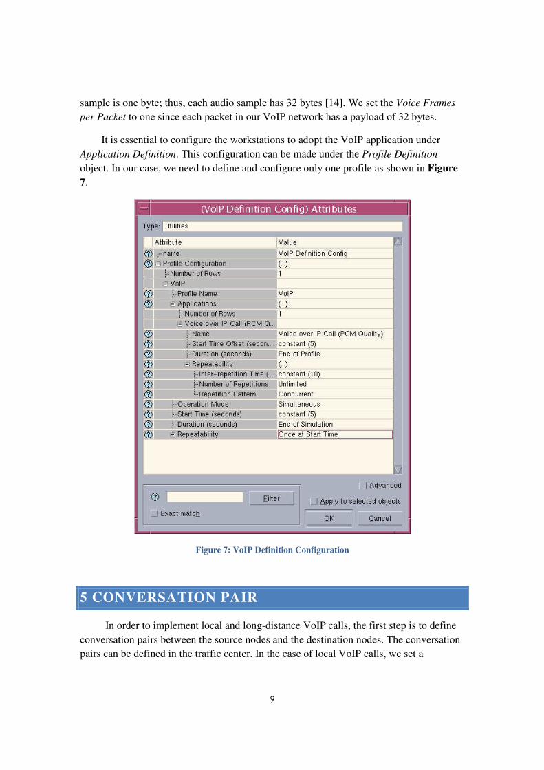
sample is one byte; thus, each audio sample has 32 bytes [14]. We set the Voice Frames
per Packet to one since each packet in our VoIP network has a payload of 32 bytes.
It is essential to configure the workstations to adopt the VoIP application under
Application Definition. This configuration can be made under the Profile Definition
object. In our case, we need to define and configure only one profile as shown in Figure
7.
Figure 7: VoIP Definition Configuration
5 CONVERSATION PAIR
In order to implement local and long-distance VoIP calls, the first step is to define
conversation pairs between the source nodes and the destination nodes. The conversation
pairs can be defined in the traffic center. In the case of local VoIP calls, we set a
Page 17
10
conversation pair between two workstations within the Vancouver Company as shown in
Figure 8. Furthermore, in the case of long-distance VoIP call, we set a conversation pair
between one workstation in the Vancouver Company and another workstation in the New
York Company as shown in Figure 9.
Figure 8: Local Conversation Pair Shown in Traffic Center
Figure 9: Long-Distance Conversation Pair Shown in Traffic Center
Page 18
11
6 DISCUSSION
This section discusses the behaviour of VoIP under different scenarios. We create
four different scenarios with names included in Table 2.
Table 2: Scenario Names
Scenario one Comparison between local and long-distance VoIP communication
Scenario two Comparison between a busy VoIP network and a non-busy VoIP network
Scenario three Observation of VoIP quality under different discard ratio (Internet Qos)
Scenario four Different encoder schemes usage and their effects on VoIP quality
It is a good idea to comprehend the definition of the parameters that we measure
from scenario one to scenario four such as jitter, end-to-end delay, packet loss and Mean
Opinion Score. Table 3 summarizes the definition of the parameters. Further information
can be reviewed in the Introduction section.
Table 3: Parameters to Measure for Scenarios
Jitter Variation in packet arrival time
End-to-End
delay
The time at which the source sends out the packets to the time the receiver
gets the packets
Packet loss Observation of VoIP quality under different discard ratio (Internet QoS)
MOS Mean Opinion Score (MOS) value represents the user satisfaction. The
higher the MOS value, the better the quality of the VoIP quality as shown in
Figure 10.
Page 19
12
Figure 10: Speech Transmission Quality and Mean Opinion Score Ratings
6.1 SCENARIO ONE:
COMPARISON BETWEEN LOCAL AND LONG-DISTANCE VOIP
COMMUNICATION
The purpose of this scenario is to compare local and long-distance VoIP calls in
term of different parameters. We create one long-distance conversation pair between the
two companies and two local conversation pairs within the Vancouver company – one
conversation pair on the same floor and one conversation pair between two different
floors as shown in Table 4.
Table 4: Conversation Pairs Set up for Scenario One
Vancouver_Floor1 workstation3 ---> Vancouver_Floor1 workstation4
Vancouver_Floor1 workstation1 ---> NewYork_Floor1 workstation1
Vancouver_Floor1 workstation2 ---> Vancouver_Floor3 workstation1
Page 20
13
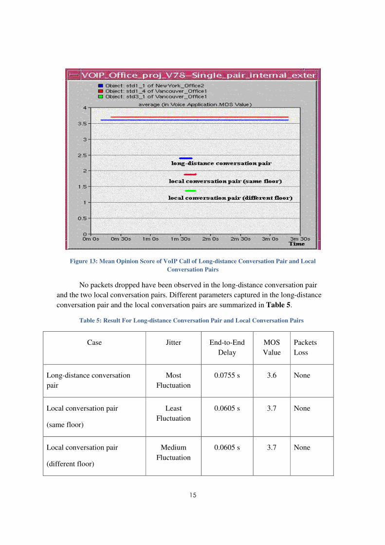
Figure 11 illustrates the jitter happens in the three conversation pairs. The blue line in
Figure 11 is the jitter in the long-distance conversation pair; whereas the red and green
lines represent the jitter happen in the local conversation pairs on the same floor and the
local conversation pair between different floors, respectively.
Figure 11: Jitter in Long-Distance Conversation Pair and Local Conversation Pairs
The long-distance conversation pair has the most fluctuating jitter; and the
conversation pair happens on the same floor within the same company introduces the
least fluctuating jitter. Jitter causes delay in the conversation. Voice packets arrived at the
receivers with more fluctuating jitter have lower voice quality. If the absolute value of
jitter is too large, then the callers and the receivers will notice the delay and the
conversation become a walkie-talkie style conversation [15].
Figure 12 shows the end-to-end delay happen in the local conversation pairs and
the long-distance conversation pair. The blue line illustrates the end-to-end delay in the
long-distance conversation pair; whereas the red and green lines show the end-to-end
delay in the local conversation pair on the same floor and the local conversation pair
between different floors, respectively.
Page 21
14
Figure 12: End-to-End Delay in Long-Distance Conversation Pair and Local Conversation Pairs
The end-to-end delay in all three cases does not exceed the time constraint – 80ms.
The end-to-end delay in the long-distance call is longer than the end-to-end delay in two
local conversation pairs. The result is reasonable as it is necessary to takes more time for
the packets to travel from the source to the destination in the long-distance VoIP
communication case.
The MOS of the long-distance conversation pair and the local conversation pairs are
shown in Figure 13. The blue line illustrates the average MOS of the long-distance
conversation pair; whereas the red and green lines show the average MOS of the local
conversation pair on the same floor and local conversation pair between different floors,
respectively.
The MOS of the local conversation pairs is higher than the long-distance
conversation pair. This means the local conversation pairs have higher VoIP speech
quality than the long-distance conversation pair.
Page 22
15
Figure 13: Mean Opinion Score of VoIP Call of Long-distance Conversation Pair and Local
Conversation Pairs
No packets dropped have been observed in the long-distance conversation pair
and the two local conversation pairs. Different parameters captured in the long-distance
conversation pair and the local conversation pairs are summarized in Table 5.
Table 5: Result For Long-distance Conversation Pair and Local Conversation Pairs
Case Jitter End-to-End
Delay
MOS
Value
Packets
Loss
Long-distance conversation
pair
Most
Fluctuation
0.0755 s 3.6 None
Local conversation pair
(same floor)
Least
Fluctuation
0.0605 s 3.7 None
Local conversation pair
(different floor)
Medium
Fluctuation
0.0605 s 3.7 None
Page 23
16
From the result summarized in Table 5, it shows that the long-distance VoIP
conversation pair tends to has more fluctuation in jitter, longer end-to-end delay and
smaller MOS value compared with the local conversation pairs. Since jitter, end-to-end
delay and MOS value are used to determine the VoIP quality; thus, the quality of long-
distance VoIP communication is not as good as the quality of local-distance VoIP
communication.
6.2 SCENARIO TWO:
COMPARISON BETWEEN A BUSY NETWORK AND A NON-BUSY VOIP
NETWORK
In scenario one, we create a non-busy VoIP network in which there is only one
long-distance conversation pair. The purpose of this scenario is to compare a busy VoIP
network with a non-busy VoIP network in term of different parameters: jitter, end-to-end
delay, packet loss, and MOS value. Furthermore, different link capacity is used in the
busy VoIP network to see the change in the aforementioned parameters.
In order to create a busy VoIP network, 15 workstations in each company are set
to communicate with 15 workstations in the second company – 15 long-distance
conversation pair. The first 15 VoIP calls start after 10 seconds and each workstation will
generate an additional call every 10 second after.
First of all, DS1 link is used to connect the subnets to the IP cloud. After that DS3
is used to replace the DS1 link to connect the subnets to the IP cloud with the same load.
The throughput of DS1 is 1.544 Mbps; whereas the throughput of DS3 is 44.736 Mbps
Figure 14 shows the overall traffic sent and received of the busy VoIP network
using DS1 link. The overall traffic received rate is slower than the overall traffic sent rate
at the time around minute one and after. The mismatch of traffic send rate and traffic
received rate implies that the DS1 link is overloaded by then.
Page 24
17
Figure 14: Overall Traffic Received Rate and Overall Traffic Sent Rate In The Busy VoIP Network
Using DS1 Link
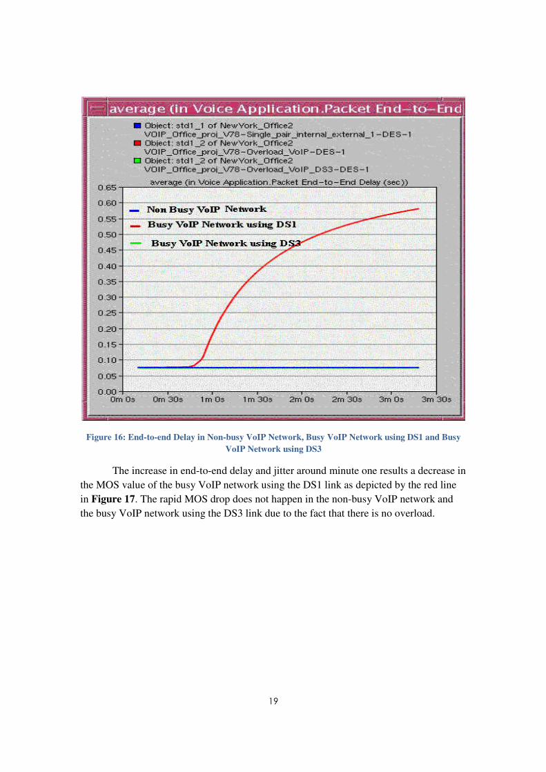
The overload slows down the throughput and increases the end-to-end delay for
the packets as depicted by the red line in Figure 16. The increase in end-to-end delay
causes many packets arriving at the destination over the time constraint, 80ms; thus,
many packets are discarded. The mismatch of traffic sent and traffic received in Figure
14 also implies packet loss.
The DS1 link is then replaced with the DS3 link in the busy VoIP network. In the
case using the DS3 link in the busy VoIP network, the overload phenomenon disappears
due to the larger capacity of the DS3 link. As a result, there is no rapid increase in end-
to-end delay and packet loss.
Due to the light traffic in the non-busy VoIP network, there is no overload
phenomenon in the network even using DS1 link.
The red and green lines in Figure 15 represent the jitter of the busy VoIP network
with DS1 link and DS3 link, respectively. The blue line shows the jitter of the non-busy
VoIP network using DS1.
Page 25
18
Figure 15: Jitter in Non-busy VoIP Network, Busy VoIP Network using DS1 and Busy VoIP Network
using DS3
Figure 15 clearly shows that the jitter rapidly increases at the time around minute
one when the DS1 link is overloaded in the busy VoIP network. This behaviour does not
show in the cases of non-busy VoIP network and the busy VoIP network using the DS3
link. Similarly, in Figure 16 there is a rapid increase in the end-to-end delay in the busy
VoIP network using DS1 link at the time around minute one due to capacity overload
causing slow throughput as mentioned previously.
Page 26
19
Figure 16: End-to-end Delay in Non-busy VoIP Network, Busy VoIP Network using DS1 and Busy
VoIP Network using DS3
The increase in end-to-end delay and jitter around minute one results a decrease in
the MOS value of the busy VoIP network using the DS1 link as depicted by the red line
in Figure 17. The rapid MOS drop does not happen in the non-busy VoIP network and
the busy VoIP network using the DS3 link due to the fact that there is no overload.
Page 27
20
Figure 17: MOS of Non-busy VoIP Network, Busy VoIP Network using DS1 and Busy VoIP Network
using DS3
The parameters captured from the non-busy VoIP network, the busy VoIP
network using the DS1 link and the busy VoIP network using the DS3 link are
summarized in Table 6.
Table 6: Result for Non-busy VoIP Network, Busy VoIP Networks using DS1 and DS3
Case Jitter End-to-End Delay MOS Value Packets Loss
Non-busy VoIP
Network
Negligible
Fluctuation
Constant 0.075
second
Constant 3.6 No Packets
Dropped
Busy VoIP
Network using DS1
Most
fluctuation
Rapidly Increase
When the Link
Overloaded
Rapidly Decrease
When the Link
Overloaded
Packets Dropped
Around One
Minute And
After
Busy VoIP
Network using DS3
Negligible
fluctuation
Constant 0.075
second
Constant 3.6 No Packets
Dropped
Page 28
21
From the result summarized in Table 6, we observe that the quality of VoIP
deteriorates as the VoIP network is getting busy. When the VoIP network becomes busy,
overload happens and causes larger fluctuation in jitter, longer end-to-end delay, lower
MOS value and more packet loss. The solution is to change the link capacity. The
replacement of DS1 link by the DS3 link eliminates the overload because the DS3 link
has much faster data rate than the DS1 link. As a result, in order to improve the voice
quality in a busy VoIP network, it is essential to use a high capacity link such as DS3,
OC24 and OC48.
6.3 SCENARIO THREE:
OBSERVATION OF VOIP QUALITY UNDER DIFFERENT DISCARD
RATIO (INTERNET QOS)
The purpose of this scenario is to observe how the Internet QoS affects the quality of
VoIP. The discard ratio is used to differentiate the Internet QoS. According to OPENT,
packet discard ratio specifies the percentage of packets dropped. It is the ratio of packets
dropped to the total packets transferred to this cloud multiplied by 100.
We start with changing the packet discard ratio into 0.5%, 4% and 6% under the
Internet Attributes of the IP cloud. From Figure 18 to Figure 21, it shows jitter, end-to-
end Delay, MOS value and packet loss corresponding to different packet discard ratios.
Page 29
22
Figure 18: Discard Ratio Comparison--Voice Application Jitter (sec). Left: Original; Right: Zoom in
Figure 19: Discard Ratio Comparison--Voice Packet End-to-End Delay (sec). Left: Original; Right:
Zoom in
Page 30
23
Figure 20: Discard Ratio Comparison--Voice Application MOS Value
Figure 21: Discard Ratio Comparison--IP Traffic Dropped (packets per sec)
Page 31
24
We create Table 7 based on parameters captured from Figure 18 to 21. This table
makes it easier to compare jitter, end-to-end delay, MOS value and packet loss under
different discard ratio.
Table 7 : Different discard ratio used and the correspondent MOS values
Case Discard
Ratio
Jitter End-to-End
Delay
Voice
Application
MOS
Packet
Loss
(packets
per sec)
Discard_Ratio-
0.5
0.5% Least
Fluctuation
Longest 3.510 1.824
Discard_Ratio-4 4% Medium
Fluctuation
Shortest 2.896 18.411
Discard_Ratio-6 6% Most
Fluctuation
Shortest 2.584 22.024
For voice application jitter, network with 6 % discard ratio has the highest jitter
fluctuation. In term of end-to-end delay, network with 6 % discard ratio has the shortest
End-to-End Delay, compared with the other two discard ratio. It indicates that network
with higher discard ratio has less end-to-end delay time. As the discard ratio increases,
more packets are discarded during transmission causing faster link throughput. The
increase in link throughput causes packets arriving at the receiver earlier than the
expected time. Early packet arrival can also deteriorate the quality of VoIP as it makes
the voice message incomprehensive.
From Table 7, it clearly shows that the higher the discard ratio in a network, the
more packet loss occurs in that network. Furthermore, the higher the discard ratio in a
network, the lower the MOS value in that network. It is reasonable as more voice packets
are discarded in a network, the voice quality is greatly deteriorated and it explains the
drop in the MOS value.
The Internet QoS affects the quality of VoIP since different Internet QoS tends to
have different packet discard ratio. Packet discard ratio can alter jitter, end-to-end delay
and packet loss which are all VoIP deterioration factors. In Table 8, we summary how
changing packet discard ratio affect VoIP deterioration factors.
Page 32
25
Table 8 : Different discard ratios used and the correspondent change of parameters
Packet Discard
Ratio
Jitter Fluctuation End-to-End Delay MOS Packet Loss
Increase Increase Decrease Decrease Increase
Decrease Decrease Increase Increase Decrease
Table 8 shows that the higher the discard ratio, the smaller the MOS value and
therefore the worse the VoIP quality.
6.4 SCENARIO FOUR:
DIFFERENT ENCODER SCHEMES USAGE AND THEIR EFFECTS ON
VOIP QUALITY
The purpose of this scenario is to verify if coding scheme would affect the quality of
VoIP. The encoder schemes we used are Algebraic Code Excited Linear Prediction
(ACELP) G 723 5.3k, Conjugate Structure Algebraic (CS-ACELP) G 729 A and PCM G
711. Figure 22 shows the average of voice MOS value for different encoder schemes.
Figure 22: Encoder scheme comparison—average (in Voice.MOS Value)
Page 33
26
The simulation result of those three encoder schemes shows that there is no
difference in jitter, end-to-end delay and packet loss. Therefore, instead of creating a
table to show four measured parameters as Table 7, we only show the MOS value in
Table 9.
Table 9: Codec Used and the correspondent MOS values
Codec MOS
ACELP G723 5.3k 2.097
CS-ACELP G 729 A 2.316
PCM G 711 2.935
Table 9 shows the Codec PCM 711 has the highest MOS value; whereas, Codec
ACELP G 723 has the lowest MOS value. It means that Codec PCM G 711 has higher
quality, compared with the other two codec. The bit rate for ACELP G 723, CS-ACELP
G 729 and PCM G711 is 5.3 Kbps, 8Kbps and 64 Kbps respectively [12]. The delay for
ACELP G 723, CS-ACELP G 729 and PCM G711 is 30 milliseconds, 10 milliseconds,
and 0.25 milliseconds. Based on the bit rate and delay for those three codec, the rating of
MOS from the simulation results makes sense because higher compression rate makes
shorter delay which leads to higher voice quality.
We summary the delay and bit rate of the three codec in Table 10. We observe
that the faster the bit rate and shorter the delay of a codec, the better the quality (MOS) of
VoIP.
Table 10: Codec Used and the correspondent parameters
Codec Bit Rate Delay MOS
ACELP G723 5.3k Low High Low
CS-ACELP G 729 A Medium Medium Medium
PCM G 711 High Low High
Page 34
27
7 CONCLUSION
VoIP will continue to be widely used in the future since it has many advantages. In this
project, we have successfully simulated a VoIP network and we have studied factors that
deteriorate the quality of VoIP such as jitter, voice end-to-end delay, packet loss and
Internet QoS. With our VoIP simulation network, we use it under four different scenarios
to study how the VoIP deterioration factors change in each scenario. We found that the
quality of VoIP depend on the distance between communication nodes. Therefore, the
quality in long-distance VoIP communication is not as good as the quality in short-
distance VoIP communication. Long-distance VoIP communication introduces longer
end-to-end delay, more jitter fluctuation, more packet loss and low MOS value, compared
with short-distance VoIP communication.
Considering the possible overload of the network capacity, we compared non-busy and
busy VoIP networks. We found that the quality of VoIP deteriorates as the VoIP network
is getting busy. When the VoIP network becomes busy, overload happens causing larger
fluctuation in jitter, longer end-to-end delay, more packet loss and lower MOS value. The
solution to fix these parameters is to change the link capacity. As a result, in order to
improve the voice quality in a busy VoIP network, it is essential to use a high capacity
link such as DS3, OC24 and OC48.
We also found that the Internet QoS affects the quality of VoIP. Poor Internet QoS
introduce higher packer discard ratio; thus, more voice packets are dropped causing the
voice message incomprehensive. High packet ratio also has effect on other VoIP
deterioration factors such as jitter, and end-to-end delay. We also explore the effect of
compression on VoIP quality by comparing the three speed codec (G 711, G723 and
G729). The simulation results of those three codec match the compression theory.
Page 35
28
8 REFERENCES
[1] Packetizer Inc., “How Does VoIP Work?” Available:
http://www.packetizer.com/ipmc/papers/understanding_VoIP/how_VoIP_works.html,
Jan. 2009 [Mar. 1, 2009]
[2] TSeyva Pte Ltd., “Advantage Disadvantage of VoIP.” Available:
http://support.tseyva.com/support/index.php?_m=knowledgebase&_a=viewarticle&kbarti
cleid=1, Aug.02, 2007 [Feb. 25, 2009]
[3] P. Curry, J. Hagedorn, J. Hermanowicz, and M. Sparks, Synchronized Voice
Broadcast Over Congested IP Networks, Dec. 1 2007
[4] 2004 Conference Proceedings. Available:
http://www.csun.edu/cod/conf/2004/proceedings/265.htm
[5] X. Chen, C. Wang, D. Xuan, Z. Li, Y. Min and W. Zhao, Survey on QoS
Management of VoIP. Fed. 03 2003
[6] Jitter. Available: http://www.en.VoIPforo.com/QoS/QoS_Jitter.php
[7] S. Kemp, E. Eng and A. Hassanali, BlueS.E.A. Semester Research Project. Available:
http://itom.fau.edu/jgoo/fa05/ISM4220/Blusea.pdf
[8] Noise and Voice Quality in VoIP Environments. Available:
http://cp.literature.agilent.com/litweb/pdf/5988-9345EN.pdf
[9] Using OPNET Modules in a Computer Networks Class at Mercer University, ASEE
Southeach Conference 2004, Donald U. Ekong, 2004
[10] The affects of different queuing disciplines over FTP, Video and VOIP performance,
International Conference on Computer System and Technologies – CompSysTech’2004,
Mitko Gospodinov, 2004
[11] Athina Markopoulou and Fouad Tobagi, Assessment of VoIP Quality over Internet
Backbones, June 25 2002
[12] Voice Coding Algorithms. Available:
http://www.nextgendc.com/?/seminar_voice_coding.htm
[13] K. Salah and A. Alkhoraidly, An OPNET-based Simulation Approach for Deploying
VoIP, International Journal of Network Management Volume 16, Issue 3, Pages 159-183
[14] Monitoring and Troubleshooting VoIP Networks with a Network Analyzer,
http://www.tamos.com/htmlhelp/voip-analysis/jitter.htm
Page 36
29
[15] T. Schueneman, “The Advantages and Disadvantages of Using Voip”, 2009.
Available: http://ezinearticles.com/?The-Advantages-and-Disadvantages-of-Using-
VoIP&id=147921
Page 37
30
9 APPENDIX I
This appendix presents the wireless workstation model (Figure 23) and the application
processor model in the wireless workstation (Figure 24) we used in the subnets (both in
Vancouver and New York company) of the network.
Figure 23: Wireless Workstation Model
Page 38
31
Figure 24: Application Processor Model


![Introduction/Motivation - Simon Fraser Universityljilja/ENSC427/Spring15/Projects/team3/ENSC...[8] S. Grafling, P. Mahonen and J. Riihijarvi, "Performance evaluation of IEEE 1609 WAVE](https://static.documents.pub/doc/80x56/5f700439eee606489707ae55/introductionmotivation-simon-fraser-ljiljaensc427spring15projectsteam3ensc.jpg)


