Environmental Effect of Climate Change Pollutants …epubs.surrey.ac.uk/842484/1/Ngene et al., 2017...

International Journal of Applied Engineering Research ISSN 0973-4562 Volume 12, Number 14 (2017) pp. 4171-4183

© Research India Publications. http://www.ripublication.com

4171

Environmental Effect of Climate Change Pollutants Loading on Structural

Steel Stresses

Ben U, Ngene 1# , Anthony N, Ede1, # #, Gideon O, Bamigboye 1, # # #, Kumar Prashant 2 and Imam Boulent 2

1 Department of Civil Engineering, Covenant University, Ota, Ogun State, Nigeria. 2 Department of Civil/Structural Engineering, University of Surrey, Guildford, United Kingdom.

*Corresponding author

#Orcid: 0000-0003-0675-7816, # #Orcid: 0000-0002-4774-2365, # # #Orcid: 0000-0002-1976-2334

Abstract

Human activities on earth it is observed is having negative

impact on the continuous existence of life on the planet. This

is as a result of build-up of gases that tend to affect life and

well-being of plants and animals including structures put in

place to support them. Structural failure as a result of pollutant

exposure does not occur unless where there is wrong design of

the structure or the owner has not carried out routine

maintenance. The effect of such loss on structure in place

need to be further studied to engender better understanding of

structural failure possibilities or its reliability. This work

looked at the effect of gases such as SO2 and humidity known

as climate change gases in the air and their effect on steel

structures, specifically bridges, in rural, urban and industrial

locations. It was shown also that for these three types of

locations, the moment resistance and shear resistance of

structures overtime will decrease by 3% and 4.6%

respectively. However, the deflection of the same structure

will increase by 1% over the same time range. The implication

will be an increase in the cost of design and construction as a

result of increased thickness of steel structures and additional

paint coating to reduce this negative effect.

Keywords: Moment resistance, Shear resistance, Deflection,

Air pollution and Dose-response function.

INTRODUCTION

Human, it has been attributed is contributing heavily to global

climate change through anthropogenic heat production and the

emission of green-house gases [1]. The influence of such

green-house gases and climate change is seen in the

deterioration of existing structures such as buildings, cultural

artefacts, coastal erosions and marine infrastructure damages

[2]. Deterioration of materials due to air pollution come at

high cost and the damage pose a long term effect on available

infrastructure provided at high cost to the economy of nations

[3]. The study estimated the deterioration of a steel bridge

overtime using the dose-response function approaches. From

this, the resistance of the structure overtime subject to such

deterioration is estimated. Generally, the research looks at the

factors that actually impact the service life existence and

progress of deterioration of structures exposed to atmospheric

weathering.

Structural failure due to pollutant loading or exposure can

only take place in case of wrong design or due to lack of

maintenance, hence generally are long term in nature.

Understanding how air quality affects the corrosion of

materials of construction especially Steel in unsheltered

condition is therefore important to both the Structural and

Environmental Engineers.

LITERATURE REVIEW

Impact of human activities on climate

Examples of attempts to control weather by human include

seeding to augment precipitation or suppress hail or lightning

or to clear fog or modify the structure and movement of

hurricanes. Man may also influence climate inadvertently

through his various actions and activities such as urbanization

and industrialization, falling of trees, farming activities,

draining of marshes or creation of artificial lake when rivers

are dammed to provide water for various uses or for

generation of hydroelectric power.

The greatest impact of man on climate is evident in urban

areas. Here, the actions of man have such a tremendous

impact on climate that the climate prevailing in urban areas is

quite distinct in character from that in the surrounding rural

areas [1].

Impact of climate on society

Changes in climate exert a lot of influence on human beings

and the degree to which a particular environment is exposed

to damage by climate reasons is termed its vulnerability. The

human nature to adapt and withstand adverse climate impacts,

however, is termed its resistance.

Studies have indicated that the ability of society to withstand

adverse climate is not a linear function of its wealth or degree

of development [4]. As observed by [5] energy, human health



4172

and comfort are more susceptible to be affected by climate

than any other factor in the physical environment. Example,

though ultraviolet rays help to form vitamin D in the skin and

devitalize bacteria and germs, they can also cause sunburn and

inflammation of the skin. In fact, ultraviolet rays coupled with

intense heat can cause cataract of the eye. On the positive

side also, fresh air, mild temperature, moderate relative

humidity and sunshine also have healing value.

Economic activities such as in manufacturing industry,

commerce, utilities, agriculture and animal husbandry,

transport and communication are all influenced to varying

degree by climate. These human economic activities can only

be successfully pursued under right climate conditions [6-8].

Climate also influences the way a house is built and the type

of dress humans wear and they vary from culture to culture

and from climate zone to another. In this regard, [9] has noted

the classification of the world into zones with respect to their

clothing requirements to meet normal human body heat

balance. Buildings location, materials choice, designs and

method of air-conditioning of structure is affected by climate

and weather conditions. In addition, however, the building

structural safety and ability to carry the stresses arising from

the prevailing climate during its anticipated lifetime must be

guaranteed [7, 5].

Since construction activities take place in outdoor conditions,

current weather condition with regard to rain, snow, high

winds, and temperature extremes can affect it adversely.

Estimates of the number of workable days for construction

purposes are made using information on the weather variables

[7].

Effect of climate change on climate parameters

temperature

The world temperature is predicted to rise over the next

century. This increase of some few degrees will be critical to

many aspects of our lives and the health of ecosystems and

agriculture [10]. By definition, the degree of hotness of a body

as measured by a thermometer is its temperature. One critical

aspect of temperature that affects large structures is seasonal

changes. Large seasonal changes in temperature impose

greater stress on buildings and structures. Generally, studies

have shown that temperature have correlation with corrosion

rates [11]. Temperature is noted to increase the rate of

reaction, though for steel the rate decrease with increase in

temperature and also dry the surface.

Rainfall

Corrosion of metals by rainfall is dependent on the pH of the

rain, intensity, duration and amount. Though rainfall acidity

is not easy to estimate, it is known from twentieth century

measurements and records according to [12]. Coal ash

present in the past century tended to make rainfall alkaline;

hence a pH value of 5.5 is used for this work. The presence of

𝑆𝑂2 decreases the pH of rain, and also causes faster chemical

attack. This can occur by the dissolution from rain acidity or

attack of dry deposition of pollutant. As reported in [13,14]

“hygroscopic 𝑆𝑂2 in the industrial atmosphere often lowers

the pH of water, wets rust layer and dissolves the initial

corrosion products of 𝛾 − 𝐹𝑒𝑜𝑜𝐻, and also promotes the phase

transformation of 𝛾 − 𝐹𝑒𝑜𝑜𝐻 to amorphous ferric

oxyhydroxide and 𝛼 − 𝐹𝑒𝑜𝑜𝐻”. This transformation for

weathering steel is known to takes place within the first three

years of exposure.

Relative humidity

Relative humidity is one of the climate parameters included in

most of the established dose-response functions. It defines the

percentage of vapour density to saturation vapour density at

any given time. For relative humidity, the transformed

variable is 𝑅ℎ60 = (𝑅ℎ − 60) when 𝑅ℎ > 60; otherwise 0 is

used in the dose-response function [15].

As indicated by [10] cycles of relative humidity causes

crystallization and dissolution, which exert stress on structural

materials in which weathering salts are present, [16,17]

concluded that at high relative humidity, 𝑆𝑂2 might form

ferrous sulphate, which would attract water and be dissolved

on steel surfaces, thereby accelerating the corrosion with little

contribution from 𝑁𝑂2.

Time of wetness

For weathering steel, the time of wetness (TOW) may be

interchangeably used with relative humidity. This is because

steel show high critical humidity for corrosion process [18].

Bartonj and Cherny [19] has shown that there is a correlation

existing between corrosion under absorbed water films and

the amount of 𝑆𝑂2 absorbed by the films over a period equal

to TOW as in

𝑓𝑑𝑟𝑦 = 𝐶[𝑆𝑂2]𝐴. 𝑇𝑂𝑊𝐵

The power functions take into consideration the nonlinearity

of this expression regarding both 𝑆𝑂2 and TOW.

The deposition of atmospheric pollutants such as sulphate

dioxide on structures such as buildings and bridges is

influenced by time of wetness or humid condition. Water

soluble gases such as 𝑆𝑂2 and other particulate matters can be

deposited more effectively under humid environment than in

dry condition.[20] concluded that when metal atoms are

exposed to an environment containing water molecule they

can give up electrons, becoming themselves positively



4173

charged ions-provided an electrical circuit can be completed

Factors affecting air quality

Chemical composition of the atmosphere is of great

importance to the corrosion process because of their

thermodynamic and kinetic effect on corroding material.

Mellanby [21] observed that the most important pollutant that

affects structural materials are sulphur dioxide and oxides of

nitrogen and their oxidation products, together with chlorides

and particulate matter. Ozone was also considered as its

presence affects the quality of the air.

Sulphur dioxide

Emission of this substance arises from man’s activities such as

in different fuel use. The observed decline in United

Kingdom of 𝑆𝑂2 emissions since 1980 has been attributed to

equal proportions to energy economies, reduction in sulphur

content of fuels, changes in fuel use patterns (e.g. to natural

gas) and industrial modernisation.

Results of site monitoring have revealed that over the past 30

years, the decrease in urban SO2 concentrations have clearly

arisen primarily from the decrease in domestic and

industrial/commercial emissions [21].

𝑆𝑂2 + 𝑁𝑂2 → 𝑆𝑂3 + 𝑁𝑂

Smoke

While the current United Kingdom average smoke

concentration of urban annual means is 17𝜇𝑔𝑚−3, that of

central London is put at 25 − 35𝜇𝑔𝑚−3. This represent a fall

from the 1960 average of 140 𝜇𝑔𝑚−3 with some areas as

high as 350𝜇𝑔𝑚−3. The consequence is that motor,

especially, diesel vehicles are often the predominant

contributor to smoke concentration.

Oxides of nitrogen

Estimates from Warren Spring laboratory [22] indicates that

United Kingdom annual emission of 𝑁𝑂𝑥 was almost flat

from 1905 to 1945 but increased by a factor of 2 to date. This

increase is attributed to increased oil consumption by the

transport sector. Peak hourly concentration are affected by

meteorological conditions and for long it is put at an average

of 60 − 80𝜇𝑔𝑚−3 for 2𝑁𝑂2 and 40 − 65𝜇𝑔𝑚−3 for 𝑁𝑂

2𝑁𝑂 + 𝑂2 → 2𝑁𝑂2

2𝑁𝑂 + 𝑂2 → 2𝑁𝑂2 − 𝑂2

Ozone

These are not considered as primary pollutants. It is produced

in high concentrations in the stratosphere by UV irradiation

and transported into the free troposphere to supplement ozone

produced there photo chemically [22]. For the United

Kingdom, the average annual concentration in urban areas

range from 20 − 40𝜇𝑔𝑚−3 while for rural area it is 40 −

60𝜇𝑔𝑚−3. For reason of area of primary production, ozone

depends on meteorological variation for its dispersal. Apart

from that, it also depends on sufficient sunlight and

favourable air mass trajectory to transport it from source to its

receptors. Hydrocarbons in the atmosphere can be oxidized

by ozone as follows:

𝑅𝐻 + 𝑂3 → 𝑅′𝐶𝐻𝑂 + 𝑂2

Carbon dioxide

This is not considered as pollutant gas. However, its presence

in the air does add to the acidity of rain water and thereby

cause some degradation to limestone and concrete.

Combustion of fossil fuels has caused a considerable increase

in atmosphere concentration of 𝐶𝑂2 from approximately

290ppm in 1870 to 340 ppm in 1985 [12]. As a result, attacks

by 𝐶𝑂2 on calcareous stones proceeds more rapidly because

the 𝐶𝑂2 concentration increase leading to a higher partial

pressure and more decay and directly because of the low pH

[22].

Dose response

Literally, this is the function that determines the impact of the

application of a certain quantity of a substance on the

receptor. Environmental impacts of dose response functions

are liberally considered as measured data are globally used to

predict equation on local scale. In this regard, dose-response

functions are geographically transferable.

Environmental parameters:

Dose-response functions include such climate data as

temperature (T), relative air humidity (Rh), gaseous emissions

in the air (𝑆𝑂2, 𝑁𝑂2 and 𝑂3) and amount of precipitation.

Difficulty in obtaining time of wetness (TOW) resulted in its

exclusion [23].

Though polluting gaseous emissions such as 𝑆𝑂2, 𝑁𝑂2and 𝑂3

were included in the statistical analysis, the negative

correlation between 𝑁𝑂2and 𝑂3 (𝑁𝑂2 level is low in rural and

high in urban atmosphere, while 𝑂3 is the reverse) is

observed. Note that it is difficult to identify the effect of 𝑁𝑂2

and 𝑂3 separately.



4174

Estimation of corrosion losses

Weathering steel, an alloy of Nickel, Copper etc. has the dose-

response function as shown for outdoor application [23].

𝐼𝑛(𝑀𝐿) = 3.54 + 0.33𝐼𝑛(𝑡) + 0.13𝐼𝑛(𝑆𝑂2) + 0.020𝑅ℎ

+ 0.059(𝑇 − 10) 𝑓𝑜𝑟 𝑇 ≤ 10℃

and

𝐼𝑛(𝑀𝐿) = 3.54 + 0.33𝐼𝑛(𝑡) + 0.13𝐼𝑛(𝑆𝑂2) + 0.020𝑅ℎ

+ 0.036(𝑇 − 10) 𝑓𝑜𝑟 𝑇 > 10℃

where t = time in years, T = Air temperature, Rh = Relative

humidity (%), [𝑆𝑂2] = 𝑆𝑂2 concentration ( 𝜇𝑔𝑚−3), [𝑁𝑂2] =

𝑁𝑂2 concentration ( 𝜇𝑔𝑚−3), 𝑂3 = 𝑂3concentration

( 𝜇𝑔𝑚−3), Rain = Quantity of Rainfall (mm), [𝐻+] =

𝐻+concentration (𝑚𝑔 𝑙⁄ )and [CL-] = CL- concentration

(𝑚𝑔 𝑙⁄ ).

Impact pathway

The [24] project identified metals (steel) as one of the

pathways of acidic emissions and precursors of photo-

oxidants effect on materials. The impact pathway follows the

following routes: discoloration, materials loss and structural

failure. Structural failure from pollutant exposure is more

noticeable where there is fundamental flaw in design or the

property does not have good routine maintenance programme.

Failure probability of corroded structures

According to [25], corrosion has many variables with

uncertain nature. For this reason, the use of probabilistic

model to describe the expected corrosion of structures is

appropriate and desirable in reliability assessment. The

reliability (probability of survival or no failure) of a structure

is defined as

𝑃𝑠 = 1 − 𝑃𝑓

Reliability and failure probability

The limit state design process is defined by the principle of

structural reliability, [26]. Two types of limit states identified

include Ultimate limit state and Serviceability limit state.

Total failure of a structure by any mechanism (fracture,

buckling, overturning etc.) is considered to be failure under

Ultimate limit state. Other forms of limit state may however

cause a structure not to be fit for purpose. The function

𝑔(𝑥) describes the limit state as

𝑔(𝑥) > 0 limit state is satisfied (safe set)

𝑔(𝑥) < 0 failure occurs (unsafe set)

𝑔(𝑥) ≥ 0 failure surface

with x a vector of statistical variable which takes into account

uncertainties.

and𝑃𝑓 = 𝑃(𝑔(𝑥) < 0) = 𝑃(𝑅 − 𝑆 < 0)

From [27] under normal distribution, the probability of failure

𝑃𝑓of a structure is calculated from

𝑃𝑓 =∅[−𝜇𝑅 − 𝜇𝐶]

√𝜎𝑅2 + 𝜎𝑆

2= ∅[−𝛽]

Where 𝜇𝑅and 𝜇𝑐 are means and

𝜎𝑅 and 𝜎𝑆are standard deviation of the load and resistance

variables and 𝑃𝑓is the cumulative density function of the

standard normal distribution.

but reliability index [𝛽]can be expressed as

𝛽 = −∅−1(𝑃𝑓)

In order to solve the probability of failure function above, the

Monte Carlo simulation or analytical methods (First Order

Reliability Method) is employed.

Code requirement for reliability

As earlier noted, the product of failure probability and cost of

failure defines the risk level or target level of reliability.

According to [28] uncertainties associated with modelling of

deteriorating structures have strong influence on management

decisions, such as when to inspect and scheduling of

maintenance and repair actions. In this regard structural

elements that are frequently inspected, show warning signs if

failure is approaching or can redistribute its loads to other

elements and hence less likely to cause loss of life at failure.

ISO 2394 [26] suggested for serviceability limit state a target

level of reliability, 𝛽 = 0 for reversible and 𝛽 = 1.5 for

irreversible limit states.

Impact of location of structure and corrosion

Steel structures are not significantly affected by rural

corrosion since high ozone level governs. However, urban

and marine corrosions are significant since sulphate and

chloride emission prevails in both environments. Kayer [29]

noted that bearing and shear prevail in high levels of corrosion

as their resistance is based on Webs (thin member) susceptible

to thickness loss effect. In the same vein, compression

members are more sensitive to corrosion since it is subject to

buckling. Adebiyi et al., [30] in his predictive model for

evaluating corrosion rate of mild steel in six environments

concluded that the mean corrosion rate using theoretical

model varied from 0.12 cm/yr (for borehole water) to 0.55

cm/yr (for H2S04).



4175

In the works of [31], on the effects of time dependent loads

and corrosion on bridge reliability, it was determined that

failure due to shear force is a more immediate threat to a

structure than due to moments.

Surveswaran et al., [32] examined the effect of corrosion

penetration in I-girder structure reliability. The result

indicates an adverse rate of corrosion for the bottom 1 4⁄ of

the web and flange. Corrosion attack was noted for top and

bottom surfaces of flanges.

Lateral torsional buckling was determined as the most critical

failure mode affecting corroded beam; followed by shear

which affect the material loss of the bottom quarter of web

and finally moment as compression flange is less significant.

METHOD AND MATERIALS

Methodology

The impact of climate change on built infrastructure analysis

is achieved in two stages of examining the appropriate Dose-

Response function for pollutants and evaluating their impact

on a railway bridge structure.

In stage one, the mean and standard deviation of the pollutant

data are obtained. From the mean, a dose-response value of

the annual material loss is calculated for weathering steel.

Evaluating the impact of climate parameters in the second

stage involves probabilistic evaluation of the time to failure of

various stages of corrosion on simply supported railway

bridge structure using the moment and shear resistance and

deflection checks.

Data

The data for this work were obtained from the work of [12] on

estimates of recession rate of limestone facades in London

over a millennium.

This inhomogeneous data involve climate and pollutant

parameters which have historic data, non-instrument and

instrument data and future projections.

The record which represents climate around London region

(Central England Temperature

Record) can be extended to Guildford which has similar

geographic and meteorological characteristics. Key to the

merger of earlier historical records with instrument data as

observed by [33] was the high regression coefficient

𝑅2 𝑜𝑓 0.73 between the data.

Theory of analysis

EFFECT OF ANALYSIS ON MATERIALS

Dose-response function and estimation of material loss

In unsheltered condition, wet deposition (through rain) of 𝑆𝑂2

is the most important pollutant parameter for weathering steel

and zinc. Several researchers have worked on the appropriate

dose-response functions that will possibly capture the adverse

effect of climate and pollutant parameters on built structures,

however, dose-response function for the calculation of a year

corrosion loss for carbon steel based on [34] is

𝑟𝑐𝑜𝑟𝑟 = 1.77[𝑆𝑂2]0.52. 𝑒𝑥𝑝(0.020𝑅ℎ+𝑓𝑠𝑡)

+ 0.102[𝐶𝐿−]0.62. 𝑒𝑥𝑝(0.033𝑅ℎ+0.040𝑇)

where 𝑓𝑠𝑡 = 0.150(𝑇 − 10)𝑤ℎ𝑒𝑛 𝑇 ≤ 10℃, 𝑜𝑡ℎ𝑒𝑟𝑤𝑖𝑠𝑒 −

0.054(𝑇 − 10), 𝑟𝑐𝑜𝑟𝑟 = first year corrosion rate of carbon

steel in 𝜇𝑚 𝑦𝑒𝑎𝑟⁄ .

The Dose-Response function above is used to determine the

thickness loss from the surface of a corroded steel structure

which depends on the parameters of interest.

BS EN ISO 9223:2012

ISO 9223 is the code for the classification, determination and

estimation of corrosion of metals. Based on comparative

estimation of the various dose-response function thickness

losses, the function for this code was chosen for the analysis.

This is because it gives the result close to the average

thickness loss calculated in this work from other functions.

The second reason for the choice of the dose-response

function for the analysis is because of the critical influence of

the parameters in the corrosion rate of metals.

Determination of corrosion rate

Determination of the corrosion rate is based on one year

exposure of metals and the measurement of the corrosion of

the standard specimens according to [34]. From this test, the

numerical values of the first year corrosion rate of different

metals under various corrosivity categories are stated.

Estimation of corrosion rate

The estimation of the one year corrosion losses for carbon

steel is based on the dose-response function as stated below:

𝑟𝑐𝑜𝑟𝑟 = 1.77[𝑆𝑂2]0.52. 𝑒𝑥𝑝(0.020𝑅ℎ+𝑓𝑠𝑡)

+ 0.102[𝐶𝐿−]0.62. 𝑒𝑥𝑝(0.033𝑅ℎ+0.040𝑇)

where𝑓𝑠𝑡 = 0.150(𝑇 − 10)𝑤ℎ𝑒𝑛 𝑇 ≤ 10℃, 𝑜𝑡ℎ𝑒𝑟𝑤𝑖𝑠𝑒 −



4176

0.054(𝑇 − 10), N =128, 𝑅2 = 0.85 and 𝑟𝑐𝑜𝑟𝑟 = first year

corrosion rate of carbon steel in 𝜇𝑚 𝑦𝑒𝑎𝑟⁄ .

Effect of Corrosion (thickness) Loss on Steel Bridge

Design of simply supported railway bridge

Using the principle of limit state, a design of beam section is

made with the ultimate limit state and checked for deflection

using the serviceability limit state.

Determination of loading

The combination of action is determined according to the

expression in equation 6.10 [26]

∑ 𝛾𝐺,𝑗𝐺𝑘,𝑗 + 𝛾𝑝𝑃 + 𝛾𝑄,1𝑄𝑘,1 + ∑ 𝛾𝑄,𝑖𝜔0,𝑖𝑄𝑘,1

𝑖>1𝑗>1

Where 𝛾𝐺and𝛾𝑄, represents the partial safety factors with

modelling uncertainty

𝐺𝑘, the characteristic value of permanent action

𝑄𝑘, the characteristic value of variable action

P, the characteristic value of a prestressing force where

applicable

𝜔0, is the combination factor for variable action

Calculation of moment and shear resistance

These are obtained using the elastic method for simply

supported structure as

Moment, 𝑀 = 𝑤 𝐿2 8⁄ and the moment of resistance for the

main girder is calculated using 𝑀𝐷 = 𝑀𝑅 𝛾𝑚𝛾𝑓3⁄ according to

clause 9.9.1.2 of [35] part 3

and

Shear Force, 𝑉 = 𝑤 𝐿 2⁄ while the shear resistance is given as

𝑉𝐷 = [𝑡𝑤 (𝑑𝑤 − ℎℎ) 𝛾𝑚𝛾𝑓3⁄ ]𝜏1 clause 9.9.2.2 [35] part 3

here w is the load in 𝐾𝑁 𝑚⁄ and L is the span length, 𝑀𝐷 is

the bending resistance, 𝑀𝑅 is the limiting moment of

resistance, 𝛾𝑚 is the safety factor and 𝛾𝑓3 is partial factor on

characteristic yield stress.

For the shear resistance 𝑉𝐷 is the shear resistance of the web

panel, 𝑡𝑤the thickness of the web, 𝑑𝑤 is the overall depth of

the girder, ℎℎ height of any opening, 𝛾𝑚 and 𝛾𝑓3 as defined

above and 𝜏1 is the limiting shear strength of the web panel.

Verification of serviceability limit state of deflection

The check is made to verify the damage that will likely

adversely affect the durability of the structure. Bridges

structures are designed so that the deflections under load do

not bear on any required clearances.

The combination actions for this check are expressed as:

∑ 𝐺𝑘,𝑗 + 𝑃 + 𝑄𝑘,1 + ∑ 𝜔0,𝑖𝑄𝑘,1

𝑖>1𝑗>1

where variables are as earlier defined.

For the verification of deflection, the equation is

𝛿 = 5𝑤𝐿4𝑥 1012 384𝐸𝐼(𝑚𝑚)⁄ < 𝐿 800⁄ (UIC

Code 776-2R, 2𝑛𝑑 𝑒𝑑 2009)

Where δ is the deflection (mm),

w = Total Load on the structure in (kN)

L = Bridge span in (mm)

E = young’s modulus (𝑁 𝑚𝑚2⁄ )

I = Second moment of area (𝑚𝑚4).

The effect of cross girder section was not considered in the

determination of the deflection of the main girder section.

RESULTS AND DISCUSSIONS

Estimation of dose-response functions

An average dose-response function was determined as in table

1 below and used in the calculation of the thickness loss in the

work. The average function is a plot of the mean of the

highest and lowest at all the points of the one year functions.

Different results obtained for different dose-response may be

attributed to the nature of analysis and the parameters input

used in various analysis. For example, while some used 𝑆𝑂2,

Relative Humidity and Temperature only in their formulation

others added the effect of 𝑂3, pH and particulate matter in the

equat



4177

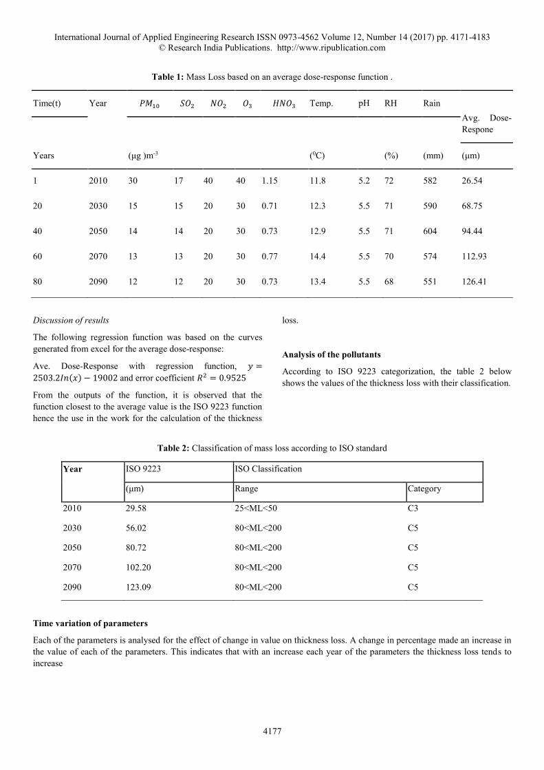
Table 1: Mass Loss based on an average dose-response function .

Time(t) Year 𝑃𝑀10 𝑆𝑂2 𝑁𝑂2 𝑂3 𝐻𝑁𝑂3 Temp. pH RH Rain

Avg. Dose-

Respone

Years

(μg )m-3 (0C) (%) (mm) (μm)

1 2010 30 17 40 40 1.15 11.8 5.2 72 582 26.54

20 2030 15 15 20 30 0.71 12.3 5.5 71 590 68.75

40 2050 14 14 20 30 0.73 12.9 5.5 71 604 94.44

60 2070 13 13 20 30 0.77 14.4 5.5 70 574 112.93

80 2090 12 12 20 30 0.73 13.4 5.5 68 551 126.41

Discussion of results

The following regression function was based on the curves

generated from excel for the average dose-response:

Ave. Dose-Response with regression function, 𝑦 =

2503.2𝐼𝑛(𝑥) − 19002 and error coefficient 𝑅2 = 0.9525

From the outputs of the function, it is observed that the

function closest to the average value is the ISO 9223 function

hence the use in the work for the calculation of the thickness

loss.

Analysis of the pollutants

According to ISO 9223 categorization, the table 2 below

shows the values of the thickness loss with their classification.

Table 2: Classification of mass loss according to ISO standard

Year ISO 9223 ISO Classification

(μm) Range Category

2010 29.58 25<ML<50 C3

2030 56.02 80<ML<200 C5

2050 80.72 80<ML<200 C5

2070 102.20 80<ML<200 C5

2090 123.09 80<ML<200 C5

Time variation of parameters

Each of the parameters is analysed for the effect of change in value on thickness loss. A change in percentage made an increase in

the value of each of the parameters. This indicates that with an increase each year of the parameters the thickness loss tends to

increase



4178

Table 3: Effect of % age change on parameters relative to 2050 values

%age change 2050 Refernce year parameters

ISO 9223

(μm)

ISO 9223

S02

(μg )m-3

Thickness Loss

(μm) Temp. (oC)

Thickness Loss

(μm) RH (%)

Thickness Loss

(μm)

DRF1(μm)

-20 11.2 21.99 10.32 28.39 56.8 18.59 29.58 29.58

-10 12.6 23.38 11.61 26.48 63.9 21.43 26.44 56.02

0 14 24.70 12.9 24.70 71 24.70 24.70 80.72

10 15.4 25.95 14.19 23.04 78.1 28.47 21.48 102.20

20 16.8 27.15 15.48 21.49 85.2 32.81 20.90 123.10

Discussion

From the table 3 above, increase in temperature does not

increase thickness loss while for other parameters, sulphur

dioxide and relative humidity, increases thickness loss with

their increase. Example, from the table, a 10% increase in 𝑆𝑂2

will cause a 5% increase in thickness loss, which for a 20mm

thick web will give rise to a reduction of 1mm thickness. A

10% increase in temperature on the other hand will cause 7%

decrease in thickness loss. Increase in relative humidity by

10% will cause a 15% increase in thickness loss. It is

therefore observed that increase in relative humidity will

increase the amount of water vapour hence dissolved 𝑆𝑂2 and

other gases and also increase in the time of wetness of

corrosive materials on the structure.

Spatial variation of parameters

In this regard, it is observed that location affects the rate of

loss of materials from steel exposed to the climate change.

Materials exposed to the rural area is least affected while

those in industrial environment is most affected as seen in

figures 1-3 below. Table 4-6 below shows the use of the ISO

9223 dose-response function to obtain the thickness losses

over time for rural, urban and industrial environments. To

obtain these values, the 𝑆𝑂2 is varied for the rural, urban and

industrial areas while the temperature and relative humidity is

kept constant. A plot of the thickness loss against time for

various environments gives the rate of corrosion.

Table 4: Rural values of SO2(2 < SO2<15)

Time Year PM10 S02 N02 O3 HN03 Temp. pH RH Rain ISO 9223

Year (μg )m-3 (0C) (%) (mm) (μm)

1 2010 30 17 40 40 1.15 11.8 5.2 72 582 29.58

20 2030 15 15 20 30 0.71 12.3 5.5 71 590 56.02

40 2050 14 14 20 30 0.73 12.9 5.5 71 604 80.72

60 2070 13 13 20

30

0.77 14.4 5.5 70 574 102.20

80 2090 12 12 20 30 0.73 13.4 5.5 68 551 123.09

Table 5: Urban values of SO2(5<SO2<100)



4179

Time Year PM10 S02 N02 O3 HN03 Temp. pH RH Rain ISO 9223 ISO 9223

Year (μg )m-3 (0C) (%) (mm) (μm) (μm)

1 2010 30 78 40 40 1.15 11.8 5.2 72 582 65.32 65.32

20 2030 15 69 20 30 0.71 12.3 5.5 71 590 58.47 123.79

40 2050 14 64 20 30 0.73 12.9 5.5 71 604 54.43 178.22

60 2070 13 60 20

30

0.77 14.4 5.5 70 574 47.58 225.80

80 2090 12 55 20 30 0.73 13.4 5.5 68 551 46.12 271.92

Table 6: Industrial values of SO2(50< SO2<400)

Time Year PM10 S02 N02 O3 HN03 Temp. pH RH Rain ISO 9223 ISO 9223

Year (μg )m-3 (0C) (%) (mm) (μm) (μm)

1 2010 30 360 40 40 1.15 11.8 5.2 72 582 144.68 144.68

20 2030 15 315 20 30 0.71 12.3 5.5 71 590 128.78 273.47

40 2050 14 295 20 30 0.73 12.9 5.5 71 604 120.49 393.96

60 2070 13 270 20

30

0.77 14.4 5.5 70 574

104.02 497.98

80 2090 12 250 20 30 0.73 13.4 5.5 68 551 101.35 599.32

Discussion

From the tables 4,5 and 6, it is shown that sulphur dioxide

corrosion is much high for industrial area than in rural

environment. The effect is therefore a higher thickness loss in

the industrial area than in the rural. The rate of corrosion is

shown to be 1.17 𝑢𝑚 𝑎⁄ , 2.58 𝑢𝑚 𝑎⁄ and 5. 68 𝑢𝑚 𝑎⁄ for rural,

urban and industrial areas respectively. This shows that 𝑆𝑂2

corrosion rate compared for rural to industrial is

approximately five times while urban compared to industrial

and rural compared to urban rate is slightly above two times

for each.

Depth of corrosion

Steel corrosion rate with time for outdoor exposure is not

constant. From ISO 9224, it is shown to decrease with

exposure by the relation:

𝐷 = 𝑟𝑐𝑜𝑟𝑟𝑜𝑠𝑖𝑜𝑛 ∗ 𝑡𝑏

Where t is the exposure time in years, 𝑟𝑐𝑜𝑟𝑟𝑜𝑠𝑖𝑜𝑛 is the rate in

the first year expressed in 𝑢𝑚 𝑎⁄ and b is the metal-

environment-time exponent, which for carbon steel is 0.026.

The following expressions show the 𝑟𝑐𝑜𝑟𝑟𝑜𝑠𝑖𝑜𝑛 used for the

determination of the depth of corrosion for the various

environments viz rural, urban and industrial.

For the rural area, 𝑟𝑐𝑜𝑟𝑟𝑜𝑠𝑖𝑜𝑛(2 < 𝑆𝑂2 < 15) =

3259.8𝐼𝑛(𝑋) − 2473

Urban environment had, 𝑟𝑐𝑜𝑟𝑟𝑜𝑠𝑖𝑜𝑛(5 < 𝑆𝑂2 < 100) =

5281.9𝐼𝑛(𝑋) − 40104

and the industrial area has,𝑟𝑐𝑜𝑟𝑟𝑜𝑠𝑖𝑜𝑛(50 < 𝑆𝑂2 < 400) =

11623𝐼𝑛(𝑋) − 88252

Effect of climate change on structures

Impact on a railway bridge structure

The following are the analysis done to calculate the effect of

material loss on the railway bridge structure. The worked

example is of a twin-track bridge spanning 36m as in SCI

Publication P318, [36]. The bridge is square at its ends and the

slab is wholly on top of the cross girders.



4180

Design parameters

The design is for 2 standard gauge tracks on straight

alignment, track speed up to 160 km/h. Access walkway is

provided on one side of the track and a continuous position of

safety on the other side. The track is located with

approximately 100 mm clearance between the outer edges of

the walkway and the inner edges of the top flange, to allow for

possible future realignment of the track.

Heavy traffic, 27 × 106 tonnes/annum was used for the

analysis.

Grade S355 steel and grade C40 reinforced concrete was used.

The plot of the effect of thickness loss on moment resistance,

shear resistance and deflection are shown in the figures 1-3

below.

Figure 1: Effect of thickness loss on moment resistance of bridge girder

Figure 2: Effect of thickness loss on shear resistance of bridge girder

y = -5396ln(x) + 99440R² = 1

y = -16206ln(x) + 181685R² = 0.9624

55500

56000

56500

57000

57500

58000

58500

59000

Mo

me

nt

Re

sist

ance

Years

Effect of Thickness Loss on Moment Resistance

Rural Environment

Urban Environment

Industrial Environment

y = -2237ln(x) + 23244R² = 0.9969

y = -3687ln(x) + 34268R² = 0.986

y = -9275ln(x) + 76711R² = 0.9951

5700

5800

5900

6000

6100

6200

6300

2009 2040 2071

She

ar R

esi

stan

ce

Years

Effect of Thickness Loss on Shear Resistance

Rural Environment

Urban Environment




4181

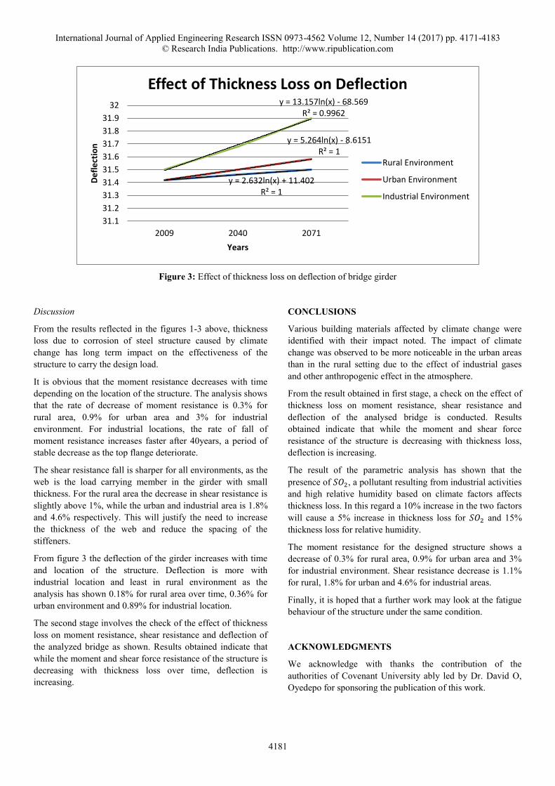
Figure 3: Effect of thickness loss on deflection of bridge girder

Discussion

From the results reflected in the figures 1-3 above, thickness

loss due to corrosion of steel structure caused by climate

change has long term impact on the effectiveness of the

structure to carry the design load.

It is obvious that the moment resistance decreases with time

depending on the location of the structure. The analysis shows

that the rate of decrease of moment resistance is 0.3% for

rural area, 0.9% for urban area and 3% for industrial

environment. For industrial locations, the rate of fall of

moment resistance increases faster after 40years, a period of

stable decrease as the top flange deteriorate.

The shear resistance fall is sharper for all environments, as the

web is the load carrying member in the girder with small

thickness. For the rural area the decrease in shear resistance is

slightly above 1%, while the urban and industrial area is 1.8%

and 4.6% respectively. This will justify the need to increase

the thickness of the web and reduce the spacing of the

stiffeners.

From figure 3 the deflection of the girder increases with time

and location of the structure. Deflection is more with

industrial location and least in rural environment as the

analysis has shown 0.18% for rural area over time, 0.36% for

urban environment and 0.89% for industrial location.

The second stage involves the check of the effect of thickness

loss on moment resistance, shear resistance and deflection of

the analyzed bridge as shown. Results obtained indicate that

while the moment and shear force resistance of the structure is

decreasing with thickness loss over time, deflection is

increasing.

CONCLUSIONS

Various building materials affected by climate change were

identified with their impact noted. The impact of climate

change was observed to be more noticeable in the urban areas

than in the rural setting due to the effect of industrial gases

and other anthropogenic effect in the atmosphere.

From the result obtained in first stage, a check on the effect of

thickness loss on moment resistance, shear resistance and

deflection of the analysed bridge is conducted. Results

obtained indicate that while the moment and shear force

resistance of the structure is decreasing with thickness loss,

deflection is increasing.

The result of the parametric analysis has shown that the

presence of 𝑆𝑂2, a pollutant resulting from industrial activities

and high relative humidity based on climate factors affects

thickness loss. In this regard a 10% increase in the two factors

will cause a 5% increase in thickness loss for 𝑆𝑂2 and 15%

thickness loss for relative humidity.

The moment resistance for the designed structure shows a

decrease of 0.3% for rural area, 0.9% for urban area and 3%

for industrial environment. Shear resistance decrease is 1.1%

for rural, 1.8% for urban and 4.6% for industrial areas.

Finally, it is hoped that a further work may look at the fatigue

behaviour of the structure under the same condition.

ACKNOWLEDGMENTS

We acknowledge with thanks the contribution of the

authorities of Covenant University ably led by Dr. David O,

Oyedepo for sponsoring the publication of this work.

y = 2.632ln(x) + 11.402R² = 1

y = 5.264ln(x) - 8.6151R² = 1

y = 13.157ln(x) - 68.569R² = 0.9962

31.1

31.2

31.3

31.4

31.5

31.6

31.7

31.8

31.9

32

2009 2040 2071

De

fle

ctio

n

Years

Effect of Thickness Loss on Deflection

Rural Environment

Urban Environment




4182

REFERENCES

[1] Ayoade, J. O., 2004, “Introduction to Climatology

for the Tropics (2nd Ed.)”, Spectrum Books Ltd.,

Nigeria.

[2] Feenstra, J. F., 1984, “Cultural Property and Air

Pollution: Damage to Monuments, Art – Objects,

Archives and Buildings due to Air Pollution,

Ministry of Housing, Physical Planning and

Environment”, the Netherlands.

[3] Ngene, B.U., (2016). "Structures in a changing

climate", LAP LAMBERT Academic Publishing,

Germany, Pp-140, ISBN-13:978-3-659-81049-7,

ISBN-10: 36598 10495 and EAN: 9783659810497.

[4] Burton, L., 1978, “Scope Workshop and

Climate/Society Interface”, Canada: Toronto.

[5] Critchfield, H. J., 1974, “General Climatology”, New

Jersey; Prientice-Hall Inc.

[6] Mather, J. R., 1974, “Climatology: Fundamentals and

Applications”, New York: Mc Graw-Hill.

[7] Smith, K. 1975, “Principles of Applied

Climatology”, New York, Mc Graw-Hill.

[8] Hobbs J. E., 1980, “Applied Climatology: A Study of

Atmospheric Resources”. Damson, Folkestone.

[9] Giffithe J. F., 1976, “Climate and the Environment:

The Atmospheric Impact”, London: Paul Elek.

[10] BrimbleCombe P, and Grossi C.M., 2007, “Damage

to Buildings from Future Climate and Pollution”.

APT Bulletin, 38, pp. 13-18.

[11] Economic Commission for Europe Air Pollution 1

Air-Borne Sulphur, Pollution Effect and Control,

Report prepared within the Framework of the

Convention on Long-range Transboundary Air

Pollution, UN Publication Geneva, 1984.

[12] Brimblecombe P., Grossi, C. M., 2008, “Millenium-

long Recession of limestone Facades in London”,

Environ Geol. 56, pp. 463-471.

[13] Wang, J. H. Wei, F. S., Chang, Y. S, Shih, H.C.

1997, “The Corrosion Mechanisms of Carbon Steel

and Weathering Steel in S02 Polluted Atmospheres”.

Materials, Chemistry and Physics 47, pp. 1-8.

[14] Misawa, T. K., Asami, K., Hashimoto, S.

Shimodaira, 1974, “The Mechanism of Atmospheric

Rusting and the Protective Amorphous Rust on Low

Alloy Steel”, Corrosion. Sci., 14, pp. 279-289

[15] Kucera V., Tidblad, J., Kreislova, K. Knotkova, D.,

Faller, M., Reiss, D., Snethlage, R. Yates, T,

Henriksen, J. Schreiner, M., Melcher, M. Ferm, M.

Lefevre, R. Kobus, J, 2007, “UN/ECE ICP Materials

Dose-Response Functions for the Multi-pollutant

Situation”. Water Air Soil Pollution: Focus 7, pp.

249-258.

[16] Arroyave, C., Morcillo, M., 1995, “The Effort of

Nitrogen Oxide in Atmospheric Corrosion of

Metals”, Corrosion Science, 37 (2), pp. 293-305.

[17] Henriksen, J. F., Rode, A, 1986, “Proc. 10th

Scandinavian Corrosion Cong., Stockholm, p. 39.

[18] Leuenberger – Minger, A. U. Buchmann, B., Faller,

M., Richner, P., M. Zobeli, Dose-response Functions

of Weathering Steel, Copper and Zinc Obtained from

a Four-year Exposure Programme in Switzerland.

Corrosion Service, 44 (2002) 675-687.

[19] Bartonj, K. Cherny, M. Z. 1980, Met., 16 (4) pp. 387.

[20] Castro, C. F, Rodrigues, J. A. F. Belzunce, O.

Canteli, Stainless Steel Rebar for Concrete

Reinforcement, 2002.

[21] Mellanby, K., 1988, “Air pollution, Acid Rain and

the Environment”, Report Number 18, Watt

Committee Report: Edited.

[22] UK Building Effects Review Group (UKBERG). The

Effect of Acid Deposition on Buildings and Building

Materials in the UK, HMSO, London. 1990.

[23] Mikhailov, A. A. 2001, Dose-Response Functions as

Estimates of the Effect of Acid Precipitation on

Material, Protection of Metals, 37 (4) pp. 357-366.

Translated from Zashchita Metallov 37 (4) (2001)

400-410 Original Russian Text Copyright @2001 by

Mikhailov.

[24] ExternE (European Commission), Assessment of

Global Warming Damages, (1998),

http://www.externeinfo/reportex/vol7.pdf

[25] Melchers, R, 2002, “Structural Reliability Analysis

and prediction”, 2nd Ed. John wiley & sons.

[26] BS EN ISO 9223, Corrosion of metals and alloys -

Corrosivity of atmospheres - Classification,

determination and estimation. The British Standard

Institute, 2012.

[28] ImramRafiq, M. Chryssanthopoulos, M. K.,

Onoufrion, T., 2004, “Performance upgrading of

concrete bridges using proactive health monitoring

methods”. Reliability Engineering and System

Safety, 86, pp. 247-256.

[29] Kayer, J. R. Nowak, A. S., 1989, “Reliability of

Corroded Steel Girder Bridges”. Structural Safety, 6,

pp, 53-63.

[30] Adebiyi, K. A, Hameed, K. A., Ajayi, E. O., 2003,

“Predictive Model for Evaluating Corrosion Rate of



4183

Mild Steel in Six Environments”, Lautech Journal of

Engineering and Technology, 1 (1), pp. 75-81.

[31] Park, C. H., 1999, “Time Dependent Reliability

models for Steel Girder Bridges”. Thesis, University

of Michigan.

[32] Sarveswaran, J., Smith, J., WandBlockley, D. I.,

1998, “Reliability of Corrosion-Damaged Steel

Structures using internal probability Theory”.

Structural Safety 20 (1998) 237-255.

[33] Van Engelen, A. F.V., Buisman,, J., Ijnsen, F., 2001,

“A Millenium of weather, winds and water in the low

counties”. In: P.D. Jones, A.E.J. Ogilvie, T.D.

Davies, K.R. Briffa, (eds). History and climate:

memories of the future? Springer, Heidelberg, pp.

101-124.

[34] BS EN ISO 9223, Corrosion of metals and alloys -

Corrosivity of atmospheres - Classification,

determination and estimation. The British Standard

Institute. 2012.

[35] BS 5400-3.,Steel, concrete and composite bridges-

Part 3: Code of practice for design of steel bridges.

The British Standard Institute. 2000.

[36] ILES, D.C., 2004, “Design Guide for Steel Railway

Bridges”. The Steel Construction Institute.

Publication, 318.

Date post:	16-May-2018
Category:	Documents
Upload:	phungkien
View:	213 times
Download:	0 times

Environmental Effect of Climate Change Pollutants …epubs.surrey.ac.uk/842484/1/Ngene et al., 2017...

Documents